parameter estimation from retarding potential analyzers in ... · thank you for everything, dr....
TRANSCRIPT
Parameter Estimation from Retarding Potential Analyzers in thePresence of Realistic Noise
Shantanab Debchoudhury
Dissertation submitted to the Faculty of theVirginia Polytechnic Institute and State University
in partial fulfillment of the requirements for the degree of
Doctor of Philosophyin
Electrical Engineering
Gregory D. Earle, ChairSrijan SenguptaWayne A. ScalesAmos L. Abbott
Ryan L. Davidson
February 15, 2019Blacksburg, Virginia
Keywords: Retarding Potential Analyzers, in-situ data in terrestrial ionosphere, impact ofnoise, uncertainty in the presence of noise, statistics guided resampling
Copyright 2019, Shantanab Debchoudhury
Parameter Estimation from Retarding Potential Analyzers in thePresence of Realistic Noise
Shantanab Debchoudhury
(ABSTRACT)
Retarding Potential Analyzers (RPA) have a rich flight heritage. These instruments arelargely popular since a single current-voltage (I-V) profile can provide in-situ measurementsof ion temperature, velocity and composition. The estimation of parameters from an RPAI-V curve is affected by grid geometries and non-ideal biasing which have been studied inthe past. In this dissertation, we explore the uncertainties associated with estimated ionparameters from an RPA in the presence of instrument noise. Simulated noisy I-V curvesrepresentative of those expected from a mid-inclination low Earth orbit are fitted with stan-dard curve fitting techniques to reveal the degree of uncertainty and inter-dependence be-tween expected errors, with varying levels of additive noise. The main motive is to provideexperimenters working with RPA data with a measure of error scalable for different geome-tries. In subsequent work, we develop a statistics based bootstrap technique designed tomitigate the large inter-dependency between spacecraft potential and ion velocity errors,which were seen to be highly correlated when estimated using a standard algorithm. Thenew algorithm - BATFORD, acronym for ”Bootstrap-based Algorithm with Two-stage Fitfor Orbital RPA Data analysis” - was applied to a simulated dataset treated with noise froma laboratory calibration based realistic noise model, and also tested on real in-flight datafrom the C/NOFS mission. BATFORD outperforms a traditional algorithm in simulationand also provides realistic in-situ estimates from a section of a C/NOFS orbit when thesatellite passed through a plasma bubble. The low signal-to-noise ratios (SNR) of measuredI-Vs in these bubbles make autonomous parameter estimation notoriously difficult. We thuspropose a method for robust autonomous analysis of RPA data that is reliable in low SNRenvironments, and is applicable for all RPA designs.

Parameter Estimation from Retarding Potential Analyzers in thePresence of Realistic Noise
Shantanab Debchoudhury
(GENERAL AUDIENCE ABSTRACT)
The plasma environment in Earth’s upper atmosphere is dynamic and diverse. Of particularinterest is the ionosphere - a region of dense ionized gases that directly affects the variabilityin weather in space and the communication of radio wave signals across Earth. Retardingpotential analyzers (RPA) are instruments that can directly measure the characteristics ofthis environment in flight. With the growing popularity of small satellites, these probes needto be studied in greater detail to exploit their ability to understand how ions - the positivelycharged particles- behave in this region. In this dissertation, we aim to understand howthe RPA measurements, obtained as current-voltage relationships, are affected by electronicnoise. We propose a methodology to understand the associated uncertainties in the estimatedparameters through a simulation study. The results show that a statistics based algorithmcan help to interpret RPA data in the presence of noise, and can make autonomous, robustand more accurate measurements compared to a traditional non-linear curve-fitting routine.The dissertation presents the challenges in analyzing RPA data that is affected by noise andproposes a new method to better interpret measurements in the ionosphere that can enablefurther scientific progress in the space physics community.

Dedication
To my mother, Nandini Debchoudhury, for being my greatest supporter; and to the magicalpeople from two magical places separated by over eight thousand miles - Kolkata and
Blacksburg.
iv

Acknowledgments
I believe that moments and memories define us. This dissertation would not have been butfor a collage of myriad moments that I have been lucky to be part of — moments of laughter,worry, exhilaration, sadness, anger and satisfaction. I would take this opportunity to thanksome of the many faces behind these moments.
I cannot but start with my advisor Dr. Gregory Earle, who has guided, encouraged, taught,supported and helped me in every phase of my graduate studies. His contribution to my life isimmeasurable that goes beyond academia from discussions spanning books, politics, historyto, both literally and figuratively, everything under the sun. An international student, newto a different country, culture and academic setup, cannot ask for a better guide and abetter teacher. Thank you for everything, Dr. Earle. I consider myself extremely fortunateto work with Srijan Da, whose statistics know-how has helped me shape this dissertation.I have felt enriched through numerous brainstorming sessions with him and I consider hima true friend, philosopher and guide. He is the Aragorn to Dr. Earle’s Gandalf. I wantto thank Dr. Wayne Scales for his lessons on the fundamentals of plasmas in space whichhave set the foundations of my knowledge in space physics. This dissertation would not havematerialized had it not been for some of the pioneering work done by Dr. Ryan Davidson,whose knowledge of RPAs was invaluable to my research. Dr. Lynn Abbott provided usefulinsights into the methodology of the problem, which helped me define a structure and thinkdeeply about many algorithmic facets. I would like to acknowledge NSF, for supporting mywork at Virginia Tech through NSF grant AGS 1242898.
I am proud to have interacted with some great people at Space@VT, which has its own uniqueplace in my collage of memories. Thank you to Karthik and Vidur for the words of wisdomin my early days here. Debbie — you are wonderful and we cannot thank you enough fortaking care of all of us at Space@VT. Thanks are in order for Stephen, Disha, Ellen, Nabil Daand Srimoyee Di. I will keep my memories of both the mindless and intellectually satisfyingconversations with Shibaji Da, who I am sure has an excellent research career ahead of him.But most of all, I will cherish my memories with Lee Kordella who has been beside mealong the way, accompanying me in the dizzying hours of night-outs. Thank you to Dr.Scott Bailey — one of the nicest persons I have met, and Dr. Scott England — for endlessconversations ranging from food to headphones to academic research.
For as long as I remember I had been in love with the institution of academics. I had alwayswanted to pursue a PhD and every decision in my life has been to meet that goal. My parentsconstantly supported me throughout my journey and even more so when I met failures alongthe way. I still remember my father encouraging me with some of my favorite food — Biryanior tandoori chicken — whenever I was down or disappointed. They made me a strong personwho can, to this day, face failures with optimism for the better. My mother is integral to
v
everything I am and the values I carry with me. My grandparents Amma and Pilu, who Iso wish lived to see me achieving many of my dreams, were part of many memories that Ican hold on to forever.
My undergraduate days at Jadavpur University contributed greatly to my making. Rohan,Rupam, Kundu, Subhro, Bagh, Bindita, Bani, Leo, Deblina, Mosha, Babu, Kot, Tapas -you all are very special to me. A big shout-out to my school friends as well — the C2group especially, from which Buro and Swastik even shared the football (not the Americanone) pitch with me at Jadavpur. Speaking about football, it is impossible not to mentionManchester United and the grit and tenacity of the legendary Sir Alex teams which hasinspired me in more ways than one in my life. Football and research will forever be with me.
And then there is my family in Blacksburg. Where do I even begin? I have seen people comeand go; I have seen the Indian and Bengali community here evolve through the years and Ihave been there to laugh and cry all along the way. Abhijit Da and Shreya Di — thank youfor many things, but most of all for providing Santa mama status to me. It saddens me thatI will probably miss a large part of Niharika’s growing up, but I am happy beyond wordsthat I was there when she was born and took her first steps. Poorna di and Sreeya di — youwere, are and will be the elder sisters I never had. Gupta da — thank you for tolerating us (:-) ) and being the guardian who had (and still has) the appropriate advice for everything !Godfather, Brato Da and Hossain Da — I wish you stayed at VT beyond just my first year.Wrik Da — my carrom and bridge partner, thank you for the guidance that I found valuablelater on. Prasen da — you brought back life into Blacksburg and gave us the PahartolirLoop as we know it. Subhradeep Da, Debarati Di, Goth Da, Avik Da, Bikram Da, Donu Da,SRC, Atashi Di — you have been wonderful seniors. Fadikar “Ramkrishna” Da and DebjitDa — pronam ! And the cricketers — Harsh, Abinash, Aniket, Appy, Arka, Kartik, Saikat— thank you for countless memories. The Indian Cricket Team does not share levels of unityas we do ! My juniors — Rounak, Ritwam, Bachha — your eccentricities are so dear to me!
And then there are those closest to me (both geographical and emotional proximity) whomanage to make you smile every day. I would not thank you, for that would be belittle yourcontribution, so I shall settle for few words. Ranit — the prankster and the most responsibleperson at the same time; Paul — the Borda and Monday-Soyabean-Curry chef; GB — myfirst junior (and hence very dear to me) at VT and barir beral; Arit — I am so happy mybrother joined VT and always remember that you are one of the most amazing persons ever;Lekha — keep us updated with the latest trend; Sreeya Di —- in addition to what I saidbefore, I want you to know that you are one of the bravest persons I have ever met.
Nath, — I miss you. Somewhere in 1309, echoes of our footsteps still ring to this day asmemories float through time ....
Shuchi, — Always !
vi
Contents
List of Figures x
List of Tables xvi
1 Introduction 1
1.1 RPA measurement . . . . . . . . . . . . . . . . . . . . . . . . . . . . . . . . 2
1.2 Effect of RPA parameters on the I-V curve . . . . . . . . . . . . . . . . . . . 6
2 The noise problem: Sources of errors 10
2.1 Sources of errors in parameter estimates . . . . . . . . . . . . . . . . . . . . 10
2.1.1 Effects of grid geometry . . . . . . . . . . . . . . . . . . . . . . . . . 10
2.1.2 Errors due to noise: The problem statement . . . . . . . . . . . . . . 12
2.2 Modeling noise . . . . . . . . . . . . . . . . . . . . . . . . . . . . . . . . . . 12
2.2.1 Uniform noise . . . . . . . . . . . . . . . . . . . . . . . . . . . . . . . 12
2.2.2 Gaussian noise model . . . . . . . . . . . . . . . . . . . . . . . . . . 13
2.3 Simulating a noise distribution from calibration data . . . . . . . . . . . . . 14
3 Error quantification for uniform noise 18
3.1 Details of the simulation study . . . . . . . . . . . . . . . . . . . . . . . . . 18
3.2 Objective of the study: A scalable guideline to expected uncertainties . . . . 22
3.2.1 Scaling Signal-to-noise ratio . . . . . . . . . . . . . . . . . . . . . . . 22
3.3 Results of the simulation study . . . . . . . . . . . . . . . . . . . . . . . . . 24
3.3.1 Characterization of errors in estimated ion temperature . . . . . . . . 25
3.3.2 Characterization of errors in estimated ion velocity . . . . . . . . . . 25
3.3.3 Characterization of errors in estimated spacecraft potential . . . . . . 26
3.3.4 Characterization of errors in composition of oxygen ions . . . . . . . 27
vii

3.3.5 Characterization of errors in combined composition of molecular ionspecies . . . . . . . . . . . . . . . . . . . . . . . . . . . . . . . . . . . 28
3.3.6 Characterization of errors in estimated ion density . . . . . . . . . . 28
3.4 Guideline to scale results . . . . . . . . . . . . . . . . . . . . . . . . . . . . . 29
3.5 Inter-dependencies between errors in parameters . . . . . . . . . . . . . . . . 32
3.5.1 A discussion on the estimation of density errors . . . . . . . . . . . . 36
3.6 Orbit coverage of simulation study . . . . . . . . . . . . . . . . . . . . . . . 36
4 Dissecting the problem: Analytical study of I-V curves 39
4.1 Why we need an analytical investigation . . . . . . . . . . . . . . . . . . . . 39
4.2 Analytical relation between errors in velocity and potential . . . . . . . . . . 41
4.3 Validating the analytical relation . . . . . . . . . . . . . . . . . . . . . . . . 44
4.4 The noise effect from an algorithm perspective . . . . . . . . . . . . . . . . . 45
5 BATFORD: An improved algorithm 48
5.1 Bootstrap method for resampling . . . . . . . . . . . . . . . . . . . . . . . . 48
5.2 BATFORD algorithm . . . . . . . . . . . . . . . . . . . . . . . . . . . . . . 50
5.2.1 BATFORD convergence criterion . . . . . . . . . . . . . . . . . . . . 54
6 Comparative studies of the new algorithm 57
6.1 A generalized dataset . . . . . . . . . . . . . . . . . . . . . . . . . . . . . . . 57
6.2 Results from the simulated dataset . . . . . . . . . . . . . . . . . . . . . . . 60
7 Analysis and Discussion 69
7.1 Summary of findings . . . . . . . . . . . . . . . . . . . . . . . . . . . . . . . 69
7.2 BATFORD convergence . . . . . . . . . . . . . . . . . . . . . . . . . . . . . 70
7.3 Case study of noise effects from simulation results . . . . . . . . . . . . . . . 73
7.4 Application of BATFORD to Flight Data . . . . . . . . . . . . . . . . . . . 78
7.4.1 Interpretation of flight data using BATFORD . . . . . . . . . . . . . 80
7.5 SenPots . . . . . . . . . . . . . . . . . . . . . . . . . . . . . . . . . . . . . . 81
viii

7.6 Applicability of BATFORD . . . . . . . . . . . . . . . . . . . . . . . . . . . 81
7.7 Practical considerations for designing a new RPA . . . . . . . . . . . . . . . 81
8 Conclusions and future work 83
8.1 Future work . . . . . . . . . . . . . . . . . . . . . . . . . . . . . . . . . . . . 84
Bibliography 86
ix
List of Figures
1.1 Cartoon describing the RPA measurement principle. . . . . . . . . . . . . . 3
1.2 Exploded view of the LAICE RPA sensor assembly. Picture taken from Fanelliet al. [21]. . . . . . . . . . . . . . . . . . . . . . . . . . . . . . . . . . . . . . 4
1.3 A sample Maxwellian distribution for ions with velocity in the satellite ramdirection, typical for ionospheric measurements. The curve is normalized sothat its total integral is unity. . . . . . . . . . . . . . . . . . . . . . . . . . . 5
1.4 Variation of measured current with varying ion density, with other parametersmentioned in the yellow text box kept constant. . . . . . . . . . . . . . . . . 6
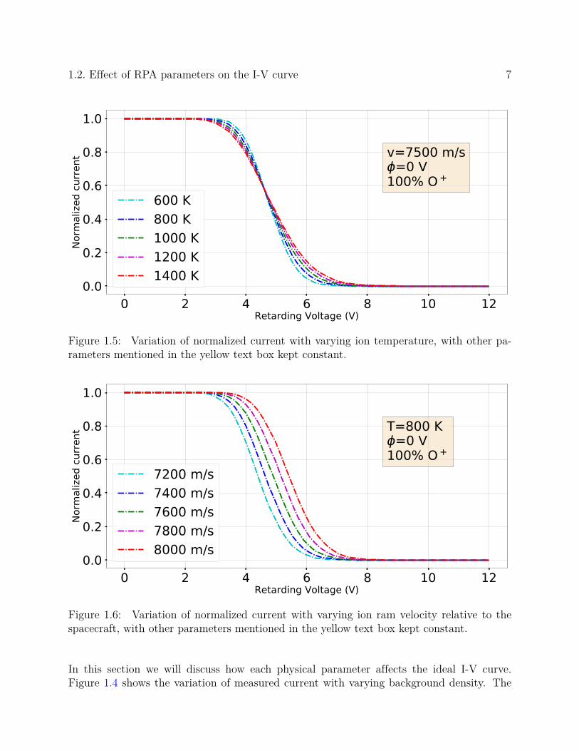
1.5 Variation of normalized current with varying ion temperature, with otherparameters mentioned in the yellow text box kept constant. . . . . . . . . . 7
1.6 Variation of normalized current with varying ion ram velocity relative to thespacecraft, with other parameters mentioned in the yellow text box kept con-stant. . . . . . . . . . . . . . . . . . . . . . . . . . . . . . . . . . . . . . . . 7
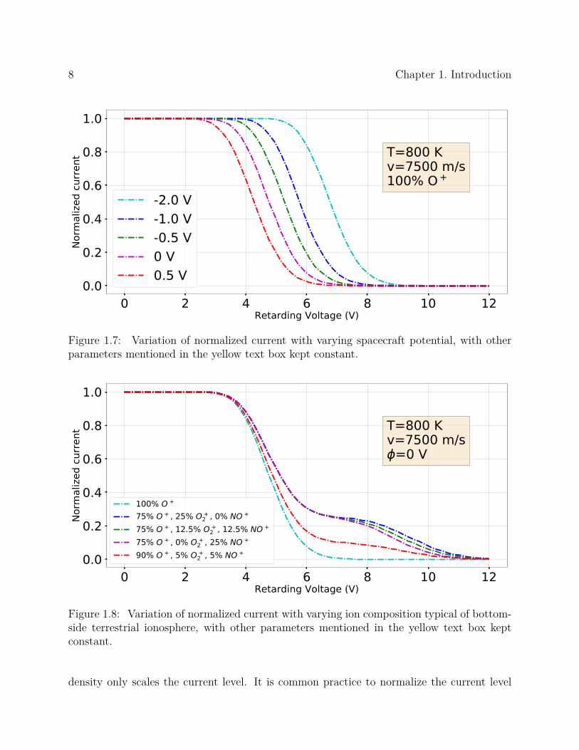
1.7 Variation of normalized current with varying spacecraft potential, with otherparameters mentioned in the yellow text box kept constant. . . . . . . . . . 8
1.8 Variation of normalized current with varying ion composition typical of bottom-side terrestrial ionosphere, with other parameters mentioned in the yellow textbox kept constant. . . . . . . . . . . . . . . . . . . . . . . . . . . . . . . . . 8
2.1 Equipotential lines inside a grid cell for (a) single, (b) woven and (c) doublethick grid geometries. Picture taken from Davidson [14]. . . . . . . . . . . . 11
2.2 Alignment (Model A) and non-alignment (model B) in a double grid geometry.Picture taken from Klenzing et al. [37]. . . . . . . . . . . . . . . . . . . . . . 11
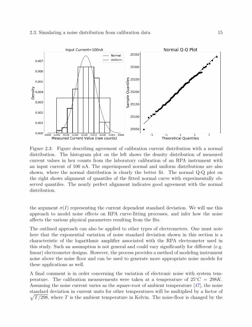
2.3 Figure describing agreement of calibration current distribution with a normaldistribution. The histogram plot on the left shows the density distribution ofmeasured current values in hex counts from the laboratory calibration of anRPA instrument with an input current of 100 nA. The superimposed normaland uniform distributions are also shown, where the normal distribution isclearly the better fit. The normal Q-Q plot on the right shows alignmentof quantiles of the fitted normal curve with experimentally observed quan-tiles. The nearly perfect alignment indicates good agreement with the normaldistribution. . . . . . . . . . . . . . . . . . . . . . . . . . . . . . . . . . . . . 15
x

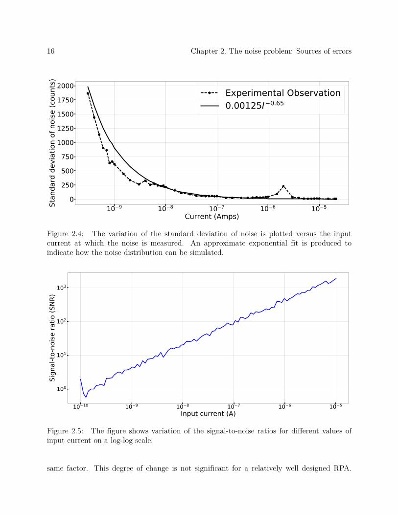
2.4 The variation of the standard deviation of noise is plotted versus the inputcurrent at which the noise is measured. An approximate exponential fit isproduced to indicate how the noise distribution can be simulated. . . . . . . 16
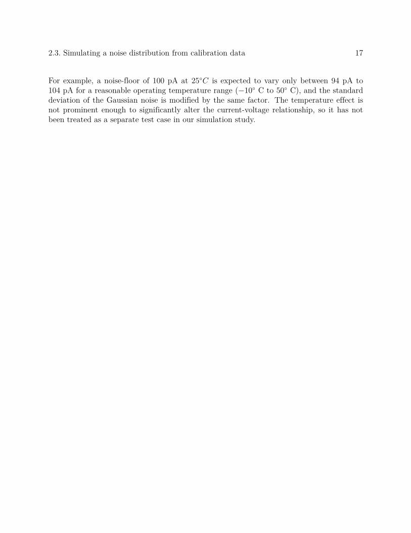
2.5 The figure shows variation of the signal-to-noise ratios for different values ofinput current on a log-log scale. . . . . . . . . . . . . . . . . . . . . . . . . . 16
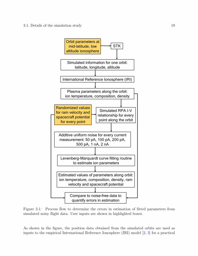
3.1 Process flow to determine the errors in estimation of fitted parameters fromsimulated noisy flight data. User inputs are shown in highlighted boxes. . . . 19
3.2 A sample I-V curve showing the definition of Imax assumed for calculatingSNR in this study. . . . . . . . . . . . . . . . . . . . . . . . . . . . . . . . . 23
3.3 Absolute errors in estimation of ion temperature as a characteristic of thebackground noise level. . . . . . . . . . . . . . . . . . . . . . . . . . . . . . . 25
3.4 Absolute errors in estimation of ram velocity as a characteristic of the back-ground noise level. . . . . . . . . . . . . . . . . . . . . . . . . . . . . . . . . 26
3.5 Absolute errors in estimation of spacecraft potential as a characteristic of thebackground noise level. . . . . . . . . . . . . . . . . . . . . . . . . . . . . . . 26
3.6 Absolute errors in estimation of percentage O+ composition as a characteristicof the background noise level. . . . . . . . . . . . . . . . . . . . . . . . . . . 27
3.7 Absolute errors in estimation of combined percentage composition of O+2 and
NO+ as a characteristic of the background noise level. . . . . . . . . . . . . 28
3.8 Percentage error in estimation of ion density as a characteristic of the back-ground noise level. . . . . . . . . . . . . . . . . . . . . . . . . . . . . . . . . 29
3.9 Illustration to show how the results presented in Figures 3.3 and 3.4, shownby the shaded yellow region, can be scaled to identify errors in temperature(panel A) and ram velocity (panel B) for an RPA with aperture area oneorder of magnitude lower, operating with a noise margin of 1 nA. . . . . . . 30
3.10 Correlation between errors in estimation of parameters. . . . . . . . . . . . . 32
3.11 Correlation between temperature and velocity errors. . . . . . . . . . . . . . 34
3.12 Correlation between potential and velocity errors. . . . . . . . . . . . . . . . 34
3.13 Correlation between O+ composition and velocity errors. . . . . . . . . . . . 35
xi

3.14 Panels (a), (b) and (c) address the issue of biases in this study caused byselection of a specific orbit. Shown above are box-plots of the input tempera-ture (a), input number density (b) and input percentage of molecular ions (c)for this single orbit study compared to the same parameters for a selectionof validation orbits. These validation orbits are phased at 6-hour intervals tospan an entire day and simulated for seasonal and solar condition variabilityto encompass a broader range of input parameters. The local times of theascending node for the validation orbits are different from the one used inthe study. The means, medians and ranges covered for each parameter showsthat our study does not suffer from significant biases. . . . . . . . . . . . . . 37
4.1 Different sections of a normalized I-V curve. . . . . . . . . . . . . . . . . . 40
4.2 The picture shows the validity of the analytically obtained relation in (4.11).The envelope denotes the potential-velocity combinations that yield a nor-malized I-V curve that lie within one noise standard deviation of a curvegenerated by an ideal reference velocity-potential pair. The line denotes theanalytical relation outlined in (4.11) for the same reference pair. The colorbardenotes the variation of Euclidean distance from the ideal reference I-V curvefor all the pairs that generates I-V curves within the noise envelope. . . . . . 43
4.3 The picture shows the validity of the analytically obtained relation in (4.11).The envelope denotes the potential-velocity combinations that yield normal-ized I-V curves that lie within one noise standard deviation of a curve gen-erated by an ideal reference velocity-potential pair at 25◦ C . The black linedenotes the analytical relation outlined in (4.12) for the same reference pairfor the entire potential range. The colorbar denotes the variation of Euclideandistance from the ideal reference I-V curve for all the pairs that generate I-Vcurves within the noise envelope. . . . . . . . . . . . . . . . . . . . . . . . . 45
4.4 Panels A, B, C and D are four representative noisy scenarios all generated fromthe same true I-V curve with 100 pA of uniform noise. The true solution (650K, 7500 m/s and -0.5 V) is shown in red, while for each case the fit solutionsare shown in yellow. The left of each panel is a slice in the velocity potentialplane while the right shows a slice in the velocity temperature plane. Thecolorbar represents the sse corresponding to the x axis and y axis pairs withthe rest of the parameters set to of the true solution. Initial conditions arethe same in all cases. Note that the fit solutions vary widely with differentnoisy representations from same distribution. . . . . . . . . . . . . . . . . . 46
5.1 A two-stage fit that analyzes one single I-V curve and is used as the core ofthe entire BATFORD procedure. . . . . . . . . . . . . . . . . . . . . . . . . 50
5.2 Outline of RPA data analysis using BATFORD. . . . . . . . . . . . . . . . . 51
xii

5.3 Options available to perform bootstrap based resampling. The results in thisdissertation has been obtained with the generalized wild bootstrap method(yellow block). However, if calibration data based noise information is avail-able to experimenters, other bootstrap schemes can be explored (as shown inthe gray blocks). . . . . . . . . . . . . . . . . . . . . . . . . . . . . . . . . . 52
5.4 The figure shows the process through which BATFORD assesses the conver-gence or stopping of the bootstrap process. The temperature (red,left axis)and velocity (blue,right axis) estimates are plotted after each bootstrap iter-ation. The shaded region shows the trajectory if more bootstrap iterationsare considered after the convergence criteria is satisfied. . . . . . . . . . . . . 55
6.1 Distribution of ion temperatures as present in the reconstructed dataset. . . 58
6.2 Distribution of ion densities as present in the reconstructed dataset. . . . . . 58
6.3 Distribution of ion velocities relative to spacecraft as present in the recon-structed dataset. . . . . . . . . . . . . . . . . . . . . . . . . . . . . . . . . . 59
6.4 Distribution of spacecraft potentials as present in the reconstructed dataset. 60
6.5 The figure shows the comparison of absolute errors in ion temperature (K) de-rived from traditional fits and from the BATFORD technique. The size of thescatter points scales linearly with the density and hence the SNR associatedwith the particular parameter combination. . . . . . . . . . . . . . . . . . . 61
6.6 The figure shows the comparison of absolute errors in ion velocity (m/s) rel-ative to the spacecraft derived from traditional fits and from the BATFORDtechnique. The size of the scatter points scales linearly with the density andhence the SNR associated with the particular parameter combination. . . . . 62
6.7 The figure shows the comparison of absolute errors in spacecraft potential(V) derived from traditional fits and from the BATFORD technique. Thesize of the scatter points scales linearly with the density and hence the SNRassociated with the particular parameter combination. . . . . . . . . . . . . 63
6.8 The standard deviations in temperature errors obtained by BATFORD plot-ted against those obtained by a traditional fit. . . . . . . . . . . . . . . . . . 64
6.9 The standard deviations in velocity errors obtained by BATFORD plottedagainst those obtained by a traditional fit. . . . . . . . . . . . . . . . . . . . 65
6.10 The standard deviations in spacecraft potential errors obtained by BATFORDplotted against those obtained by a traditional fit. . . . . . . . . . . . . . . 66
xiii

6.11 The median percentage improvement of BATFORD compared to a traditionalalgorithm is plotted for increasing density, binned into 5 density categories.The plot shows that when the background density and SNR increase, theperformance of BATFORD approaches that of a traditional method, and forlow density BATFORD offers a significant improvement. . . . . . . . . . . . 67
7.1 The figure shows convergence errors for a low density case. The y -axisgives the percentage of noisy I-V profiles at every bootstrap iteration (≥ 50)where temperature (red) and velocity (blue) convergences are achieved. Thepercentage is based on 100 noisy instances for each point plotted. . . . . . . 72
7.2 The figure shows convergence errors for a high density case. The y -axisgives the percentage of noisy I-V profiles at every bootstrap iteration (≥ 50)where temperature (red) and velocity (blue) convergences are achieved. Thepercentage is based on 100 noisy instances for each point plotted. . . . . . . 72
7.3 Panel A shows the normalized noise-free current in black along the rightaxis for an I-V curve. The red and blue lines show the noise added to thecurve for the cases that had the most accurate (blue) and least accurate(red) inferred temperatures. The noise added as a percentage of the noise-free current is read from the left axis for these two cases. The highlightedrectangular patch shows a region important to temperature estimation wherethe derivatives with respect to temperature shown in panel B are also high.Important locations are demarcated by points in Panel B while dotted verticallines map these regions to the plot in Panel A. . . . . . . . . . . . . . . . . . 74
7.4 Panel A shows the normalized noise-free current in black along the right axisfor the I-V curve. The red and blue lines show the noise added to the curve forthe cases that had the most accurate (blue) and least accurate (red) inferredvelocities. The noise added as a percentage of the noise-free current is readfrom the left axis for these two cases. The highlighted rectangular patchshows one region important to velocity estimation because the derivatives ofthe normalized I-V with respect to velocity (shown in panel B) are large. Themaximum of the derivative is shown in panel B occurs at Q0 and the verticaldotted line maps this location on the plot in Panel A. . . . . . . . . . . . . 76
xiv
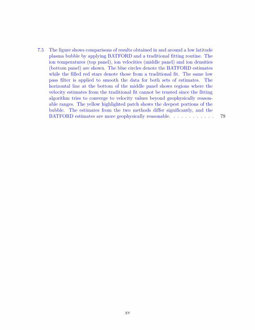
7.5 The figure shows comparisons of results obtained in and around a low latitudeplasma bubble by applying BATFORD and a traditional fitting routine. Theion temperatures (top panel), ion velocities (middle panel) and ion densities(bottom panel) are shown. The blue circles denote the BATFORD estimateswhile the filled red stars denote those from a traditional fit. The same lowpass filter is applied to smooth the data for both sets of estimates. Thehorizontal line at the bottom of the middle panel shows regions where thevelocity estimates from the traditional fit cannot be trusted since the fittingalgorithm tries to converge to velocity values beyond geophysically reason-able ranges. The yellow highlighted patch shows the deepest portions of thebubble. The estimates from the two methods differ significantly, and theBATFORD estimates are more geophysically reasonable. . . . . . . . . . . . 79
xv

List of Tables
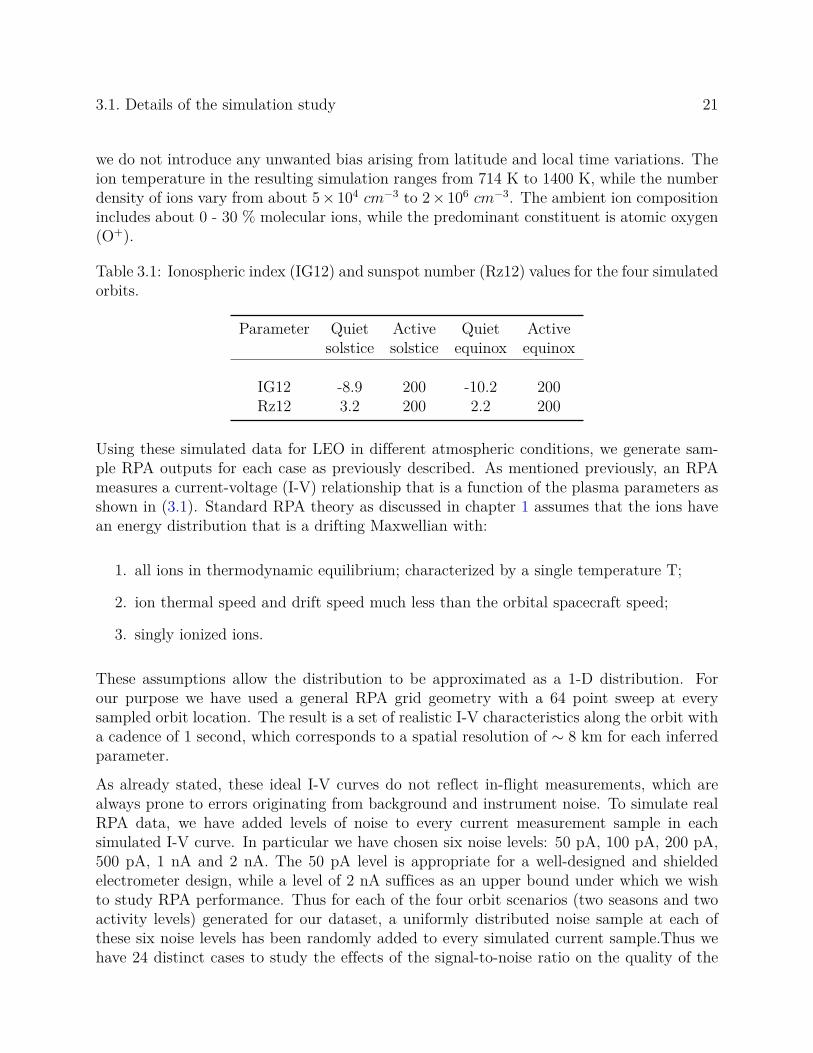
3.1 Ionospheric index (IG12) and sunspot number (Rz12) values for the four sim-ulated orbits. . . . . . . . . . . . . . . . . . . . . . . . . . . . . . . . . . . . 21
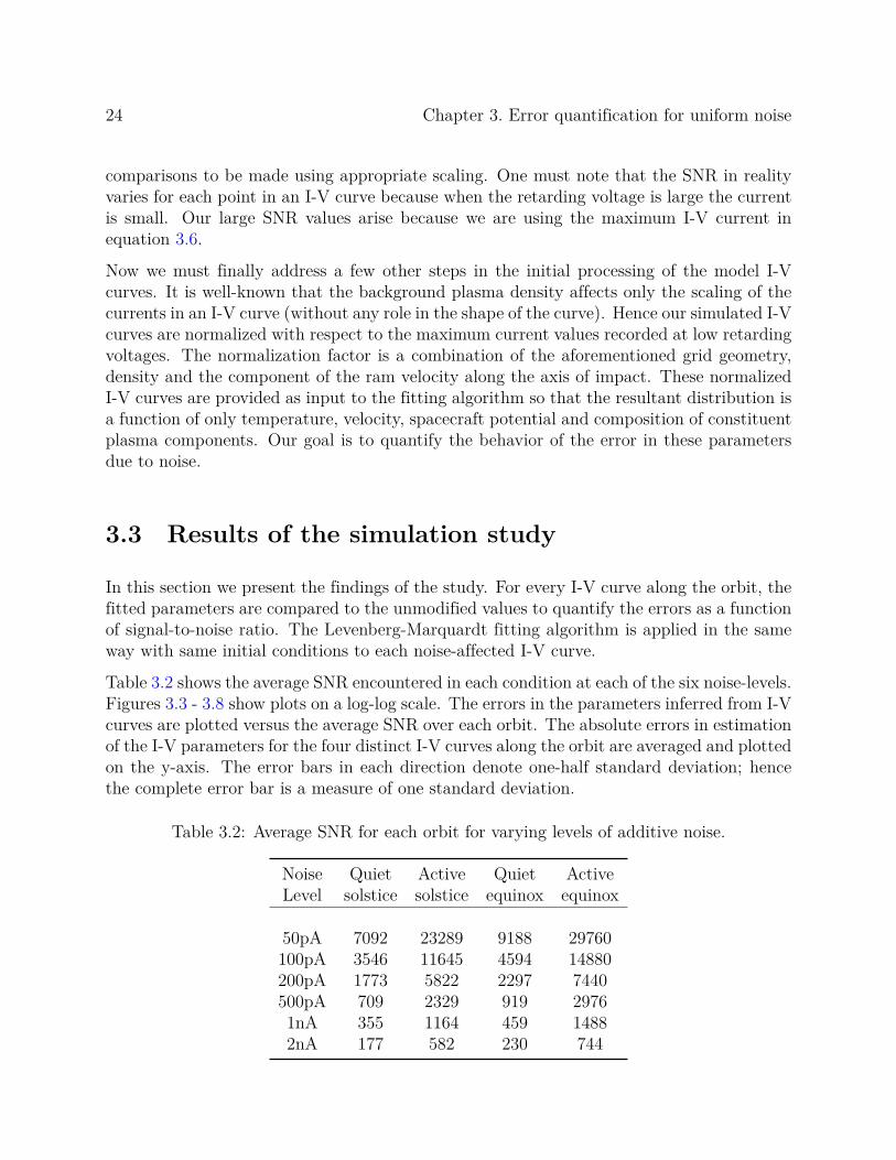
3.2 Average SNR for each orbit for varying levels of additive noise. . . . . . . . . 24
3.3 Average error in temperature, velocity and potential for an RPA design withsmaller aperture and 1 nA noise margin. . . . . . . . . . . . . . . . . . . . . 31
3.4 Average error in temperature, velocity and potential for an RPA design withsmaller aperture and 50 pA noise margin. . . . . . . . . . . . . . . . . . . . 31
6.1 Statistics for parameters in the dataset. . . . . . . . . . . . . . . . . . . . . . 59
xvi

List of Abbreviations
BATFORD Bootstrap-based Algorithm with Two-stage Fit for Orbital RPA Data analysis
C/NOFS Communications/Navigation Outages Forecast Satellite
I-V curve Current - Voltage curve
RPA Retarding Potential Analyzer
sse sum-squared errors
xvii

Chapter 1
Introduction
Ever since the late 1950s when Sputnik became the first artificial satellite to be launched intospace, the modern era of space science was ushered in - an era which has seen unprecedentedcapabilities to make measurements in space. Important scientific discoveries have been madein the near-Earth environment and in the wide realm beyond. Many of the foundationaltheories that had been based on years of astronomical and radio based observations fromscientists and hobbyists alike were tested and space agencies over the world competed forprominence in the space-race.
Fast forward to the dawn of the new century, in which technology has grown significantly.This is the age of miniaturization, where small instruments are made possible because oflow power microelectronic parts. Space science and exploration are no longer restrictedto high budget missions. CubeSats, with dimensions of tens of centimeters, can be builtfrom commercial off-the-shelf instruments. Students are encouraged to participate - spaceexploration has indeed spread its reach. CubeSats have rapidly grown in popularity, and nowbeing built in many countries by disparate institutions and space-based private companies,with missions that monitor diverse aspects of many regions in the vast extent of space.
The retarding potential analyzer, known as an RPA - is the focus of this dissertation, andhas its own place in history. Since Marconi sent the first radio waves for trans-Atlantic com-munication and Appleton confirmed the presence of a conducting layer with high densitiesof charged particles, scientists strove to understand the multifaceted dynamic nature of thenewly discovered ”ionosphere”. In-situ measurement of the ion population using RPAs datesback to work done in the 50s and 60s by Hinteregger [27], Hinteregger et al. [28], Whipple[55], Hanson and McKibbin [24], Hanson et al. [25], Anderson et al. [1] and Knudsen [38].The use of electrical systems to measure the flux of charged particles had been previouslypopularized by Mott-Smith and Langmuir [45] - the RPA was an extension of the conceptinitially designed to function as ion traps [55]. The popularity of RPAs increased with itsunique ability to make measurements of numerous ion parameters from a single current volt-age relationship. RPAs were subsequently flown on satellite missions such as Sputnik 3 [55],Atmospheric Explorer [29, 34], Dynamics Explorer [26], the Defense Meteorological SatelliteProgram [49], the Republic of China Satellite (ROCSAT) [57] and the Communications/-Navigation Outages Forecast Satellite [15].
RPAs have contributed to a number of discoveries in the ionosphere throughout the years.We are now in an era where the popularity of CubeSat missions is creating more flight
1
2 Chapter 1. Introduction
opportunities for RPAs. These smaller mission platforms pose new challenges, one of whichis understanding our instruments better. A large number of missions have been proposed inthe last decade that carry RPAs and drift meters [10, 44, 54], many of which are scheduled tolaunch soon. Understanding uncertainties in RPA measurements in therefore of paramountimportance; it is a problem that needs detailed attention in this age of miniaturization.Building on this historical perspective to motivate the reader, we proceed to a detaileddiscussion of RPAs.
1.1 RPA measurement
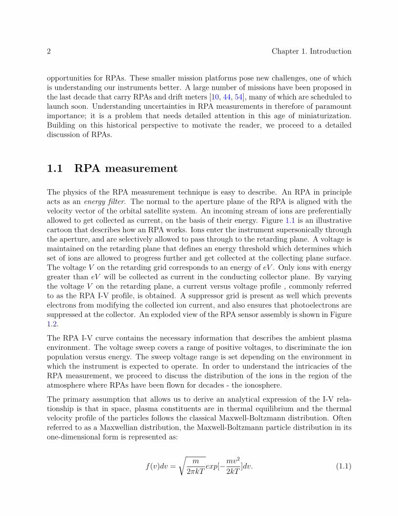
The physics of the RPA measurement technique is easy to describe. An RPA in principleacts as an energy filter. The normal to the aperture plane of the RPA is aligned with thevelocity vector of the orbital satellite system. An incoming stream of ions are preferentiallyallowed to get collected as current, on the basis of their energy. Figure 1.1 is an illustrativecartoon that describes how an RPA works. Ions enter the instrument supersonically throughthe aperture, and are selectively allowed to pass through to the retarding plane. A voltage ismaintained on the retarding plane that defines an energy threshold which determines whichset of ions are allowed to progress further and get collected at the collecting plane surface.The voltage V on the retarding grid corresponds to an energy of eV . Only ions with energygreater than eV will be collected as current in the conducting collector plane. By varyingthe voltage V on the retarding plane, a current versus voltage profile , commonly referredto as the RPA I-V profile, is obtained. A suppressor grid is present as well which preventselectrons from modifying the collected ion current, and also ensures that photoelectrons aresuppressed at the collector. An exploded view of the RPA sensor assembly is shown in Figure1.2.
The RPA I-V curve contains the necessary information that describes the ambient plasmaenvironment. The voltage sweep covers a range of positive voltages, to discriminate the ionpopulation versus energy. The sweep voltage range is set depending on the environment inwhich the instrument is expected to operate. In order to understand the intricacies of theRPA measurement, we proceed to discuss the distribution of the ions in the region of theatmosphere where RPAs have been flown for decades - the ionosphere.
The primary assumption that allows us to derive an analytical expression of the I-V rela-tionship is that in space, plasma constituents are in thermal equilibrium and the thermalvelocity profile of the particles follows the classical Maxwell-Boltzmann distribution. Oftenreferred to as a Maxwellian distribution, the Maxwell-Boltzmann particle distribution in itsone-dimensional form is represented as:
f(v)dv =
√m
2πkTexp[−mv2
2kT]dv. (1.1)
1.1. RPA measurement 3
Incoming ions
with energies:
E3 > E2 > E1
energy: E3
energy: E2
energy: E1
Aperture plane
Retarding plane at voltage V.
Allows ions with energy more than eV.
E3 > eV > E2 > E1
Collector plane
measures current
Suppressor plane
for varying V
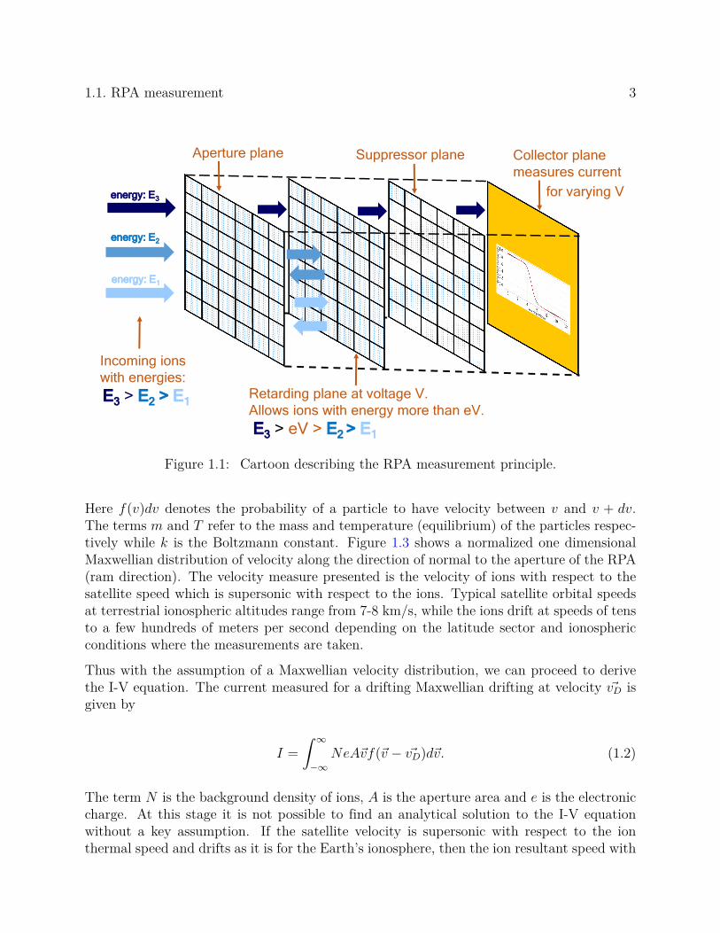
Figure 1.1: Cartoon describing the RPA measurement principle.
Here f(v)dv denotes the probability of a particle to have velocity between v and v + dv.The terms m and T refer to the mass and temperature (equilibrium) of the particles respec-tively while k is the Boltzmann constant. Figure 1.3 shows a normalized one dimensionalMaxwellian distribution of velocity along the direction of normal to the aperture of the RPA(ram direction). The velocity measure presented is the velocity of ions with respect to thesatellite speed which is supersonic with respect to the ions. Typical satellite orbital speedsat terrestrial ionospheric altitudes range from 7-8 km/s, while the ions drift at speeds of tensto a few hundreds of meters per second depending on the latitude sector and ionosphericconditions where the measurements are taken.
Thus with the assumption of a Maxwellian velocity distribution, we can proceed to derivethe I-V equation. The current measured for a drifting Maxwellian drifting at velocity vD isgiven by
I =
∫ ∞
−∞NeAvf(v − vD)dv. (1.2)
The term N is the background density of ions, A is the aperture area and e is the electroniccharge. At this stage it is not possible to find an analytical solution to the I-V equationwithout a key assumption. If the satellite velocity is supersonic with respect to the ionthermal speed and drifts as it is for the Earth’s ionosphere, then the ion resultant speed with

4 Chapter 1. Introduction
Figure 1.2: Exploded view of the LAICE RPA sensor assembly. Picture taken from Fanelliet al. [21].
respect to the spacecraft in the ram direction is far greater in magnitude than the transversecomponents. We call the generalized velocity in the ram direction vz, and the plasma flowin this direction is vD,z, which in the satellite reference frame is vplasma = vsat − vD,z. Whatthis assumption implies is that cross-track velocities (perpendicular to the ram direction) aresmall, so that all of the cross-track population is collected. Retardation takes place in theram direction only. In practice the aperture is constructed to be slightly smaller in diameterthan the collector, to ensure that all of the cross-track ions are collected.
The current is computed from the in-track component of velocity. For voltage V on theretarding grid, the minimum energy vmin that an ion must have to pass through and getcollected is:
1
2mv2min = eV (1.3)
=⇒ vmin =√
2eVm
. (1.4)

1.1. RPA measurement 5
4500 5500 6500 7500 8500 9500Velocity (m/s)
0.00000.00010.00020.00030.00040.00050.00060.0007
Prob
abilit
y de
nsity
func
tion
f(v)
Figure 1.3: A sample Maxwellian distribution for ions with velocity in the satellite ramdirection, typical for ionospheric measurements. The curve is normalized so that its totalintegral is unity.
Thus the integration of the distribution shown in Figure 1.3 must be run in the ram directionfrom vmin to ∞. We also add a transparency coefficient Tr to equation (1.2); it is a geo-metric term that dictates the cumulative optical transparency of the RPA grids. With thismodification to equation (1.2), the current expression is reduced to just the ram directionand takes the form:
I =
∫ ∞
vmin
TrNeAvzf(vz − vD,z)dvz. (1.5)
This can now be solved analytically using equation 1.2 to yield the generalized currentexpression for one species, given by Whipple [55] and Knudsen [38]:
I(V ) = TreANvplasma[1
2+
1
2erf(κ) +
vmp
2√πvplasma
exp(−κ2)], (1.6)
where,
vmp =
√2kT
m, (1.7)
κ =vplasma
vmp
−√
eV
kT. (1.8)

6 Chapter 1. Introduction
In literature, vmp is the classical most probable velocity of the Maxwellian thermal distribu-tion. From equation 1.6, one can see that the I-V curve is dependent on the equilibrium iontemperature T, the velocity of the plasma with respect to the satellite in the ram directionvplasma (or simply v henceforth), the ion density N and the concerned ion species given byits mass m. If the spacecraft is charged at a potential ϕ relative to the plasma, then theequation is obtained by replacing V by V + ϕ. When multiple species are present, the col-lector current is simply a superimposition of all the current contributions. Finally, it is alsonecessary to include a factor of cos θ with the ram velocity component in the scaling term inequation (1.6) where θ is the small misalignment of the aperture normal and the spacecraftvelocity vector.
A single RPA I-V curve can be analyzed via curve-fitting to obtain the ion temperature,density, ram velocity, spacecraft potential and composition. It is also assumed for thederivation of the I-V equation that the background ionosphere does not change significantlyin the course of one retarding voltage sweep. While this approximation holds for most ofthe low and mid-latitude regions, it is often violated in the very dynamic high latitude andpolar caps. The most common technique to analyze the I-V curve is non-linear fitting. ALevenberg-Marquardt [41] algorithm is the most popular technique to interpret results froman RPA.
1.2 Effect of RPA parameters on the I-V curve
0 2 4 6 8 10 12Retarding Voltage (V)
05
10152025303540
Curre
nt (n
A)
T=800 Kv=7500 m/s
=0 V100% O +
104 cm 3
3 × 104 cm 3
5 × 104 cm 3
8 × 104 cm 3
105 cm 3
Figure 1.4: Variation of measured current with varying ion density, with other parametersmentioned in the yellow text box kept constant.
1.2. Effect of RPA parameters on the I-V curve 7
0 2 4 6 8 10 12Retarding Voltage (V)
0.0
0.2
0.4
0.6
0.8
1.0
Norm
alize
d cu
rrent
v=7500 m/s=0 V
100% O +
600 K800 K1000 K1200 K1400 K
Figure 1.5: Variation of normalized current with varying ion temperature, with other pa-rameters mentioned in the yellow text box kept constant.
0 2 4 6 8 10 12Retarding Voltage (V)
0.0
0.2
0.4
0.6
0.8
1.0
Norm
alize
d cu
rrent
T=800 K=0 V
100% O +
7200 m/s7400 m/s7600 m/s7800 m/s8000 m/s
Figure 1.6: Variation of normalized current with varying ion ram velocity relative to thespacecraft, with other parameters mentioned in the yellow text box kept constant.
In this section we will discuss how each physical parameter affects the ideal I-V curve.Figure 1.4 shows the variation of measured current with varying background density. The
8 Chapter 1. Introduction
0 2 4 6 8 10 12Retarding Voltage (V)
0.0
0.2
0.4
0.6
0.8
1.0
Norm
alize
d cu
rrent
T=800 Kv=7500 m/s100% O +
-2.0 V-1.0 V-0.5 V0 V0.5 V
Figure 1.7: Variation of normalized current with varying spacecraft potential, with otherparameters mentioned in the yellow text box kept constant.
0 2 4 6 8 10 12Retarding Voltage (V)
0.0
0.2
0.4
0.6
0.8
1.0
Norm
alize
d cu
rrent
T=800 Kv=7500 m/s
=0 V
100% O +
75% O + , 25% O +2 , 0% NO +
75% O + , 12.5% O +2 , 12.5% NO +
75% O + , 0% O +2 , 25% NO +
90% O + , 5% O +2 , 5% NO +
Figure 1.8: Variation of normalized current with varying ion composition typical of bottom-side terrestrial ionosphere, with other parameters mentioned in the yellow text box keptconstant.
density only scales the current level. It is common practice to normalize the current level
1.2. Effect of RPA parameters on the I-V curve 9
by the maximum current so that the variation of current in equation 1.6 is restricted to theexpression in the parenthesis, which varies from 1 to 0.
Figures 1.5, 1.6, 1.7 and 1.8 describe the variation of the normalized current with respect totemperature, velocity, potential and composition. It is interesting to note that the effect ofvelocity and potential are similar, which shall be addressed in the course of the dissertation.Composition effects are manifested as presence of multiple ”humps” which correspond tothe Maxwellian peaks in the thermal distribution of the different species. The hump-likefeatures occur at voltages where the current drops significantly. It is important to highlightthe effects of all these parameters on the I-V profile as they are key to understanding manyof the aspects presented in this dissertation.
Armed with the knowledge of the physical characteristics and operational theory of RPAs,we can now investigate the practical aspects of their operation and data interpretation. Inchapter 2 we will delve deeper into the the source of uncertainty in the RPA measurementsand introduce the readers to the focus of the dissertation - the uncertainties introduced byelectronic noise.
The dissertation discusses the intricacies of analyzing data from orbital retarding potentialanalyzers in the ionosphere when noise becomes important. Throughout the rest of the text,we shall focus on the impact of noise on the estimated parameters both quantitatively andqualitatively. The dissertation attempts to help experimentalists interpret expected errorsfrom RPAs due to noise, and also provides insight into how RPA data can be interpretedthrough improved data analysis techniques applicable for all RPA designs. The conclusionsdrawn also show evidence that future RPA designs can be improved, and provide guidelineson how noise affects RPA current measurements.

Chapter 2
The noise problem: Sources of errors
2.1 Sources of errors in parameter estimates
2.1.1 Effects of grid geometry
As is the case for every instrument, the theoretically expected performance is not observed inreality. A number of factors are present contribute to the departure from the ideal behavior.Much of the prior work in this regard has been done by Chao and Su [8], Chao et al. [9],Klenzing et al. [36] and Davidson [14].
The presence of grids introduces inherent discrepancies between the measured and theoreticalcurrent for several reasons. The grids are constructed from a mesh of wires that are of finitethickness. Particles entering the RPA aperture must pass through a series of grids, so someparticles inevitably hit the grids. Optical transparency (the Tr factor in equation (1.6)) takesinto account particles that strike the front of the grids, but there are many particles whichstrike the sides of the grid as well. This grid-loss effect suppresses the theoretically expectedcollected current.
One of the assumptions in deriving the RPA I-V equation is that the potential is uniformthroughout the gridded plane. This is not the case in reality because the potential on thewires is higher than the potential in the space between the wires. Thus there is a ”leakage”of ions with energy less than the stopping potential (velocity less than vmin) that artificiallyincreases the collected current at each retarding voltage step.
In addition to leakage there is also a competing ”lensing” effect. The asymmetry in potentialbetween the grid wires sets up an electrical field in the grid plane that directs ions towardsthe center. This contributes to currents that are not expected from an ideal Maxwelliandistribution. The leakage effect can be partially mitigated by a double-grid system. Davidsonet al. [13] and Davidson and Earle [12] discuss the effects of flat, woven and double-thickgrids on the errors in estimated parameters. Intentionally mis-aligned grids (Figure 2.2) canhelp combat the lensing effect, but they reduce the optical transparency even further. Theangle of attack (θ) of the incoming particles also affects the extent of errors that are expecteddue to grid geometry and alignment.
The leakage, lensing and other effects that distort the I-V characteristics for RPAs produce
10

2.1. Sources of errors in parameter estimates 11
Figure 2.1: Equipotential lines inside a grid cell for (a) single, (b) woven and (c) doublethick grid geometries. Picture taken from Davidson [14].
Figure 2.2: Alignment (Model A) and non-alignment (model B) in a double grid geometry.Picture taken from Klenzing et al. [37].

12 Chapter 2. The noise problem: Sources of errors
errors that modify the solutions obtained for the density, ion velocity, ion temperature, andspacecraft potential. Another contamination effect has not been considered in the literature- this is the effect of electronic noise.
2.1.2 Errors due to noise: The problem statement
The focus of this dissertation is to comprehensively understand a major source of error thatis inherently associated with any instrument - electronic noise. These errors can be reducedbut not eliminated by designing an advanced instruments with less baseline noise, so it isstill important to understand the extent of noise effects in RPA data analysis.
Random fluctuations in the collector current are the manifestation of electronic noise. Varia-tion of the ambient system temperature can modify these fluctuations which we collectivelyrefer to as thermal noise. Shot noise [4] may be potentially important as well, especiallyin low density scenarios when the ion currents are small. Another significant contributioncomes from the quantization error in digitally recording the measured currents and appliedretarding voltages. The process of instrument calibration, in which a calibration profile isestablished to map from a known input current to the measured observed current, also in-troduces a form of calibration offset. Imperfect measurements during calibration are alsoconsidered to be noise. This is because the measured level 0 instrument data is convertedfrom raw to engineering units using the calibration profile that is at best an average descrip-tion of the generalized behavior.
The investigation and simulation results in this dissertation we will address the followingquestions:
1. How does the level of uncertainty in each parameter estimated in RPA data analysischange both qualitatively and quantitatively with the level of noise?
2. How does the effect of noise compare to the general effects of the grid geometry on theestimates?
3. Is there a way to improve the accuracy of estimates from measurements that are affectedby noise?
2.2 Modeling noise
2.2.1 Uniform noise
A simplistic approach to simulate the electronic noise added to an idealized I-V curve is toassume a uniform distribution of noise. The basic idea stems from the fact that the RPA
2.2. Modeling noise 13
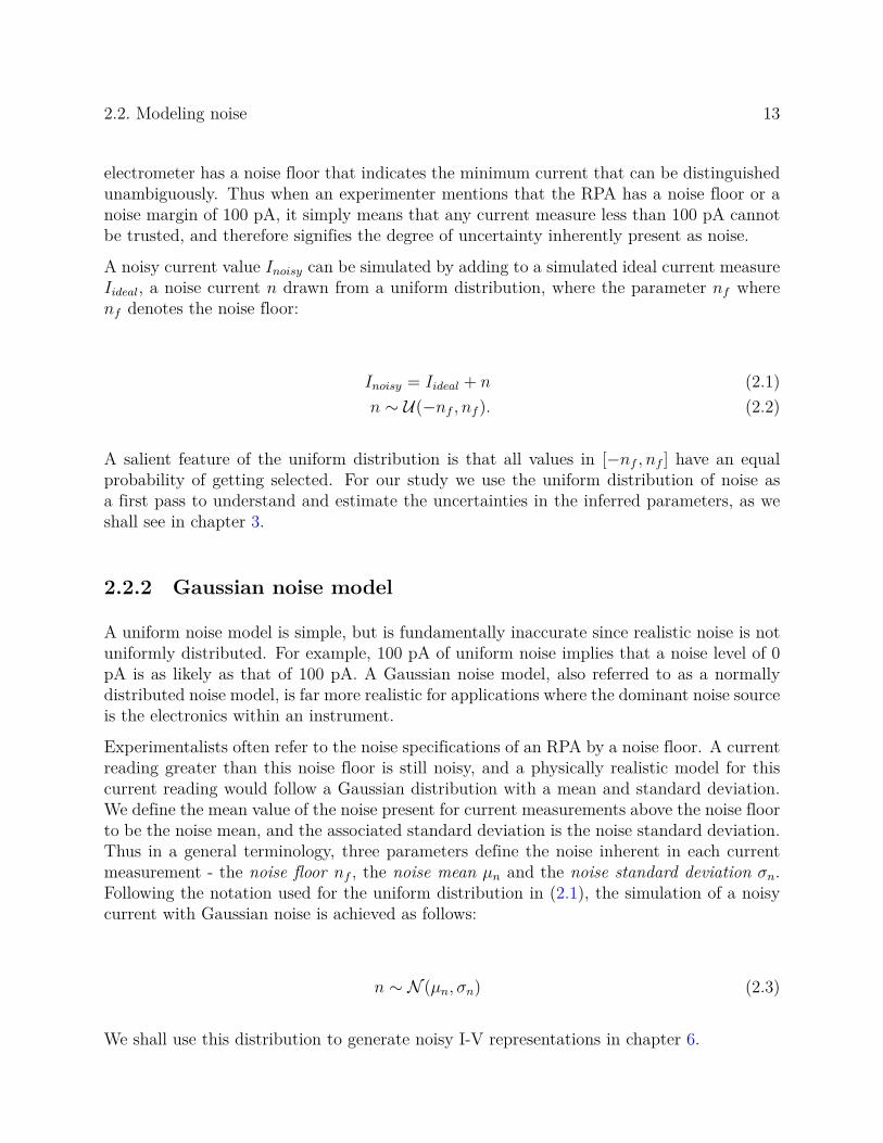
electrometer has a noise floor that indicates the minimum current that can be distinguishedunambiguously. Thus when an experimenter mentions that the RPA has a noise floor or anoise margin of 100 pA, it simply means that any current measure less than 100 pA cannotbe trusted, and therefore signifies the degree of uncertainty inherently present as noise.
A noisy current value Inoisy can be simulated by adding to a simulated ideal current measureIideal, a noise current n drawn from a uniform distribution, where the parameter nf wherenf denotes the noise floor:
Inoisy = Iideal + n (2.1)n ∼ U(−nf , nf ). (2.2)
A salient feature of the uniform distribution is that all values in [−nf , nf ] have an equalprobability of getting selected. For our study we use the uniform distribution of noise asa first pass to understand and estimate the uncertainties in the inferred parameters, as weshall see in chapter 3.
2.2.2 Gaussian noise model
A uniform noise model is simple, but is fundamentally inaccurate since realistic noise is notuniformly distributed. For example, 100 pA of uniform noise implies that a noise level of 0pA is as likely as that of 100 pA. A Gaussian noise model, also referred to as a normallydistributed noise model, is far more realistic for applications where the dominant noise sourceis the electronics within an instrument.
Experimentalists often refer to the noise specifications of an RPA by a noise floor. A currentreading greater than this noise floor is still noisy, and a physically realistic model for thiscurrent reading would follow a Gaussian distribution with a mean and standard deviation.We define the mean value of the noise present for current measurements above the noise floorto be the noise mean, and the associated standard deviation is the noise standard deviation.Thus in a general terminology, three parameters define the noise inherent in each currentmeasurement - the noise floor nf , the noise mean µn and the noise standard deviation σn.Following the notation used for the uniform distribution in (2.1), the simulation of a noisycurrent with Gaussian noise is achieved as follows:
n ∼ N (µn, σn) (2.3)
We shall use this distribution to generate noisy I-V representations in chapter 6.

14 Chapter 2. The noise problem: Sources of errors
2.3 Simulating a noise distribution from calibration data
In order to properly quantify the distribution of noise expected from an instrument, onemust take into account the laboratory bench calibration data for the instrument. While itcan be argued that the space environment produces a completely different and challengingnoisy environment for the instrument, the laboratory calibration of an instrument providesuseful insight into the uncertainty associated with a measurement. A calibration curve isused to convert raw digital RPA data (obtained in hex counts) to analog current values.The process of converting a digital count reading to an analog value using a fitted curveimparts some small quantization errors. The distribution of these calibration noise errorscan be obtained from the instrument calibration data, which are generally obtained in idealsettings with high precision instrumentation.
In our venture to simulate a realistic noise distribution, we wish to see if calibration datafrom a laboratory tested RPA does indeed resemble a Gaussian distribution. To test ourhypothesis we use bench test calibration data from the RPA described by Fanelli et al. [21] tomodel the noise distribution. On investigation of the calibration readings, it is seen that theerror in the calibrated current measurement approximately follows a Gaussian distribution.In Figure 2.3 the observed raw counts from a series of measurements for a randomly selectedinput current are plotted. The histogram of these measured noisy current in raw countsfor the input analog current shows deviations (noise) that are well represented by a normaldistribution. The quantiles of the measured sample current distribution are also shown inthe Q-Q plot [22] in the right panel of the figure. They closely align with that of a thenormal distribution, as seen from the linear trend line.
We characterize the parameters of the normal distribution, using the noise mean and stan-dard deviation. The mean approximately fluctuates around 0, so we choose the noise meanto be 0. The standard deviations observed for every input current are plotted in Figure 2.4,and an approximate experimental fit (of the form σn = AIB) is shown. Note that the noisestandard deviation fit exceeds experimentally observed values around 1 nA, which representcurrent values expected for very low densities (∼ 103 cm−3). For simulation purposes, a stan-dard deviation of this functional form would thus represent worst case scenarios since moresimulated noise is likely to be added for low current values. Since the standard deviation ofthe noise is found to be dependent on the current measure at which it is added, the signalto noise ratio (SNR = Iideal/σn) is plotted in Figure 2.5 as a function of the input currentwhere both axes are logarithmic. Thus, referring back to equation (2.3), the obtained noisedistribution is given as:
n(I) ∼ N (0, σ(I)) (2.4)σ(I) = 1.25× 10⁻³I−0.65 (2.5)
where N represents a normal distribution with the first argument denoting 0 mean, and
2.3. Simulating a noise distribution from calibration data 15
Figure 2.3: Figure describing agreement of calibration current distribution with a normaldistribution. The histogram plot on the left shows the density distribution of measuredcurrent values in hex counts from the laboratory calibration of an RPA instrument withan input current of 100 nA. The superimposed normal and uniform distributions are alsoshown, where the normal distribution is clearly the better fit. The normal Q-Q plot onthe right shows alignment of quantiles of the fitted normal curve with experimentally ob-served quantiles. The nearly perfect alignment indicates good agreement with the normaldistribution.
the argument σ(I) representing the current dependent standard deviation. We will use thisapproach to model noise effects on RPA curve-fitting processes, and infer how the noiseaffects the various physical parameters resulting from the fits.
The outlined approach can also be applied to other types of electrometers. One must notehere that the exponential variation of noise standard deviation shown in this section is acharacteristic of the logarithmic amplifier associated with the RPA electrometer used inthis study. Such an assumption is not general and could vary significantly for different (e.g.linear) electrometer designs. However, the process provides a method of modeling instrumentnoise above the noise floor and can be used to generate more appropriate noise models forthese applications as well.
A final comment is in order concerning the variation of electronic noise with system tem-perature. The calibration measurements were taken at a temperature of 25◦C = 298K.Assuming the noise current varies as the square-root of ambient temperature [47], the noisestandard deviation in current units for other temperatures will be multiplied by a factor of√
T/298, where T is the ambient temperature in Kelvin. The noise-floor is changed by the
16 Chapter 2. The noise problem: Sources of errors
10 9 10 8 10 7 10 6 10 5
Current (Amps)
0
250
500
750
1000
1250
1500
1750
2000
Stan
dard
dev
iatio
n of
noi
se (c
ount
s)
Experimental Observation0.00125I 0.65
Figure 2.4: The variation of the standard deviation of noise is plotted versus the inputcurrent at which the noise is measured. An approximate exponential fit is produced toindicate how the noise distribution can be simulated.
10 10 10 9 10 8 10 7 10 6 10 5
Input current (A)
100
101
102
103
Sign
al-to
-noi
se ra
tio (S
NR)
Figure 2.5: The figure shows variation of the signal-to-noise ratios for different values ofinput current on a log-log scale.
same factor. This degree of change is not significant for a relatively well designed RPA.
2.3. Simulating a noise distribution from calibration data 17
For example, a noise-floor of 100 pA at 25◦C is expected to vary only between 94 pA to104 pA for a reasonable operating temperature range (−10◦ C to 50◦ C), and the standarddeviation of the Gaussian noise is modified by the same factor. The temperature effect isnot prominent enough to significantly alter the current-voltage relationship, so it has notbeen treated as a separate test case in our simulation study.
Chapter 3
Error quantification for uniform noise
The first step in understanding the impact of noise is to quantify the degree of uncertaintyassociated with estimated parameters. The primary goal of this chapter is to obtain a betterunderstanding of the performance of an RPA in the space environment in the presence ofbackground noise. Much of the content of this chapter is reproduced from Physics of Plasmas24, 042902 (2017) with the permission of AIP Publishing [16]. We simulate RPA data in low-altitude regions where the ion composition includes both atomic and molecular ions. Thiscontributes to an increasing number of factors which define a fairly complicated current-voltage relationship at a given location in the flight path. The presence of noise adds to theuncertainty and stimulates further study, because RPA data analysis involves curve-fittingto infer various plasma parameters. We estimate the errors and deviation expected in theparameter fits with varying levels of noise in different geomagnetic environments. The trendsin the errors to the fit may help future studies by providing a degree of confidence in theinferred parameters given a realistic model for instrument noise. Understanding the accuracyand sensitivity of a standard RPA design will ultimately lead to a better understanding ofthe space environment.
3.1 Details of the simulation study
In order to collect realistic model data representative of a flight RPA we simulate an orbitcharacterized by the desired altitude and inclination. Figure 3.1 is a flowchart that describesthe entire process of a simulating realistic orbit and estimating errors in the fitted parametersfrom the I-V curves expected from RPA measurements in this orbit. We have chosen a mid-inclination orbit with very low altitude of 270 km. While such an orbit is too low to bestable without spacecraft propulsion, it ensures that multiple ion species will be present, soit generalizes the result. Mid-inclination orbits are common for cubesats deployed from theInternational Space Station (ISS), and also those deployed from the second stage of ISS-servicing missions. Higher altitude cubesat orbits are more common, but our results caneasily be scaled for these cases. The orbit parameters are set as inputs to a System Tool-Kit(STK™) orbit generator, and the corresponding geographical locations along the flight pathare obtained for a full orbit at a 1 minute cadence. These values are then interpolated toestimate the latitude and longitude measurements at every second of a full orbit sweep. Atypical orbit has period of roughly 93 minutes, or 5580 seconds in flight.
18
3.1. Details of the simulation study 19
Orbit parameters at
mid-latitude, low
altitude ionosphere
STK
Simulated information for one orbit:
latitude, longitude, altitude
International Reference Ionosphere (IRI)
Plasma parameters along the orbit:
ion temperature, composition, density
Randomized values
for ram velocity and
spacecraft potential
for every point
Simulated RPA I-V
relationship for every
point along the orbit
Additive uniform noise for every current
measurement: 50 pA, 100 pA, 200 pA,
500 pA, 1 nA, 2 nA
Levenberg-Marquardt curve fitting routine
to estimate ion parameters
Estimated values of parameters along orbit:
ion temperature, composition, density, ram
velocity and spacecraft potential
Compare to noise-free data to
quantify errors in estimation
Figure 3.1: Process flow to determine the errors in estimation of fitted parameters fromsimulated noisy flight data. User inputs are shown in highlighted boxes.
As shown in the figure, the position data obtained from the simulated orbits are used asinputs to the empirical International Reference Ionosphere (IRI) model [2, 3] for a practical
20 Chapter 3. Error quantification for uniform noise
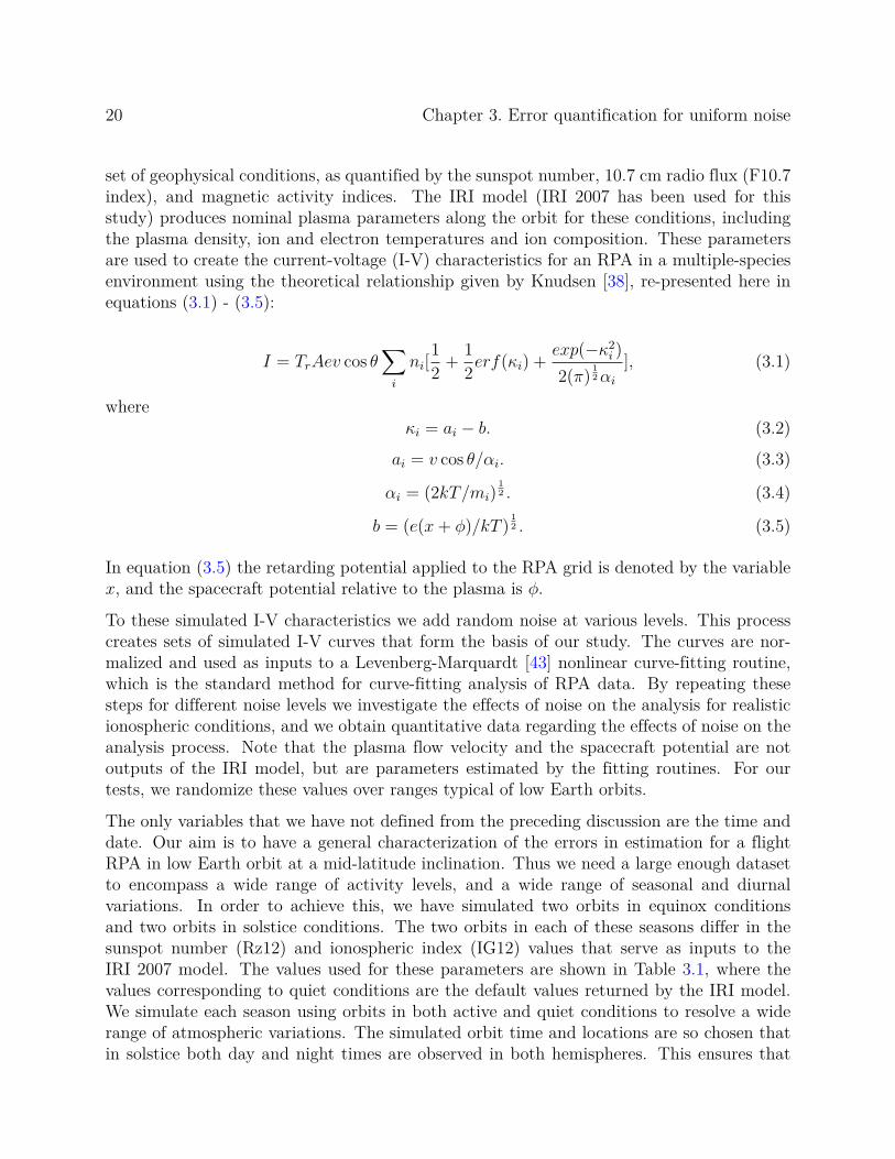
set of geophysical conditions, as quantified by the sunspot number, 10.7 cm radio flux (F10.7index), and magnetic activity indices. The IRI model (IRI 2007 has been used for thisstudy) produces nominal plasma parameters along the orbit for these conditions, includingthe plasma density, ion and electron temperatures and ion composition. These parametersare used to create the current-voltage (I-V) characteristics for an RPA in a multiple-speciesenvironment using the theoretical relationship given by Knudsen [38], re-presented here inequations (3.1) - (3.5):
I = TrAev cos θ∑i
ni[1
2+
1
2erf(κi) +
exp(−κ2i )
2(π)12αi
], (3.1)
whereκi = ai − b. (3.2)
ai = v cos θ/αi. (3.3)
αi = (2kT/mi)12 . (3.4)
b = (e(x+ ϕ)/kT )12 . (3.5)
In equation (3.5) the retarding potential applied to the RPA grid is denoted by the variablex, and the spacecraft potential relative to the plasma is ϕ.
To these simulated I-V characteristics we add random noise at various levels. This processcreates sets of simulated I-V curves that form the basis of our study. The curves are nor-malized and used as inputs to a Levenberg-Marquardt [43] nonlinear curve-fitting routine,which is the standard method for curve-fitting analysis of RPA data. By repeating thesesteps for different noise levels we investigate the effects of noise on the analysis for realisticionospheric conditions, and we obtain quantitative data regarding the effects of noise on theanalysis process. Note that the plasma flow velocity and the spacecraft potential are notoutputs of the IRI model, but are parameters estimated by the fitting routines. For ourtests, we randomize these values over ranges typical of low Earth orbits.
The only variables that we have not defined from the preceding discussion are the time anddate. Our aim is to have a general characterization of the errors in estimation for a flightRPA in low Earth orbit at a mid-latitude inclination. Thus we need a large enough datasetto encompass a wide range of activity levels, and a wide range of seasonal and diurnalvariations. In order to achieve this, we have simulated two orbits in equinox conditionsand two orbits in solstice conditions. The two orbits in each of these seasons differ in thesunspot number (Rz12) and ionospheric index (IG12) values that serve as inputs to theIRI 2007 model. The values used for these parameters are shown in Table 3.1, where thevalues corresponding to quiet conditions are the default values returned by the IRI model.We simulate each season using orbits in both active and quiet conditions to resolve a widerange of atmospheric variations. The simulated orbit time and locations are so chosen thatin solstice both day and night times are observed in both hemispheres. This ensures that
3.1. Details of the simulation study 21
we do not introduce any unwanted bias arising from latitude and local time variations. Theion temperature in the resulting simulation ranges from 714 K to 1400 K, while the numberdensity of ions vary from about 5× 104 cm−3 to 2× 106 cm−3. The ambient ion compositionincludes about 0 - 30 % molecular ions, while the predominant constituent is atomic oxygen(O+).
Table 3.1: Ionospheric index (IG12) and sunspot number (Rz12) values for the four simulatedorbits.
Parameter Quiet Active Quiet Activesolstice solstice equinox equinox
IG12 -8.9 200 -10.2 200Rz12 3.2 200 2.2 200
Using these simulated data for LEO in different atmospheric conditions, we generate sam-ple RPA outputs for each case as previously described. As mentioned previously, an RPAmeasures a current-voltage (I-V) relationship that is a function of the plasma parameters asshown in (3.1). Standard RPA theory as discussed in chapter 1 assumes that the ions havean energy distribution that is a drifting Maxwellian with:
1. all ions in thermodynamic equilibrium; characterized by a single temperature T;
2. ion thermal speed and drift speed much less than the orbital spacecraft speed;
3. singly ionized ions.
These assumptions allow the distribution to be approximated as a 1-D distribution. Forour purpose we have used a general RPA grid geometry with a 64 point sweep at everysampled orbit location. The result is a set of realistic I-V characteristics along the orbit witha cadence of 1 second, which corresponds to a spatial resolution of ∼ 8 km for each inferredparameter.
As already stated, these ideal I-V curves do not reflect in-flight measurements, which arealways prone to errors originating from background and instrument noise. To simulate realRPA data, we have added levels of noise to every current measurement sample in eachsimulated I-V curve. In particular we have chosen six noise levels: 50 pA, 100 pA, 200 pA,500 pA, 1 nA and 2 nA. The 50 pA level is appropriate for a well-designed and shieldedelectrometer design, while a level of 2 nA suffices as an upper bound under which we wishto study RPA performance. Thus for each of the four orbit scenarios (two seasons and twoactivity levels) generated for our dataset, a uniformly distributed noise sample at each ofthese six noise levels has been randomly added to every simulated current sample.Thus wehave 24 distinct cases to study the effects of the signal-to-noise ratio on the quality of the

22 Chapter 3. Error quantification for uniform noise
estimated parameters: ion density, velocity in the ram direction, spacecraft potential, iontemperature and composition.
3.2 Objective of the study: A scalable guideline to ex-pected uncertainties
It must be noted that different RPAs are designed in different ways, so that the spacingbetween grids, grid geometry, aperture size, sweep times, and number of points per sweepvary for different instruments. These factors have various impacts on the data quality,and have been discussed by other authors [8, 9, 13, 36]. While these design choices certainlyinfluence the outcome of the analysis for any particular RPA, they do so in predictable ways.For example, increasing the aperture size increases the currents to the RPA collector at allretarding voltages, thus increasing the signal to noise ratio (SNR). Similarly, using more I-Vsamples in each retarding voltage sweep improves the accuracy of the Levenberg-Marquardtfits for any I-V curve, at the expense of spatial or temporal resolution since a larger numberof samples slows the sampling rate for quality measurements from any electrometer circuit.
Given these design variables it is not possible to carry out a study like ours for every possi-ble RPA design. Our goal is therefore to quantify errors in RPA analysis for an instrumentrepresenting the current state-of-the-art for RPAs small enough to be flown on nano-satelliteplatforms [21]. By quantifying errors for such an instrument we provide a means for exper-imenters to better understand and quantify (with appropriate scaling) the veracity of theirparticular measurements.
3.2.1 Scaling Signal-to-noise ratio
We present the errors in estimation of the parameters as functions of the signal-to-noise ratio,which we define as the ratio of the ideal current to the noise current. In this SNR definitionwe choose the signal level to be the maximum value (Imax) of the simulated noise-free currentreading at the beginning of the plateau of an I-V curve (see Figure 3.2).
Thus the signal-to-noise ratio is obtained as:
SNR =Imax
Inoise, (3.6)
where Inoise is the corresponding noise level added to the current readings. To understandthe rationale behind such a definition we note that the maximum current recorded by theRPA current at a very low retarding grid potential (∼0 V) tends to
Imax = TreAN0v, (3.7)

3.2. Objective of the study: A scalable guideline to expected uncertainties 23
Imax
Plateau of I-V curve
Figure 3.2: A sample I-V curve showing the definition of Imax assumed for calculating SNRin this study.
where Tr is the grid transparency coefficient, e is the electron charge, A is the collectionarea, N0 is the background ion density and v is the ram velocity. The assumption holds forlarge values of v/
√2kTm
(T being the ion temperature, m the ion mass and k the Boltzmannconstant) for normal incidence of ions. These are valid assumptions for most RPAs flown inthe ionospheric environment.
For our study and for all the results presented henceforth, we have chosen 4 grids with atransparency of 0.81 for each so that Tr = 0.814. The aperture area A is 3.17 × 10⁻³ m−2,so equation 3.7 becomes
Imax = 1.36× 10⁻³eN0v. (3.8)
The specific parameters given above allow the SNR value used for our study to be generalizedand scaled for other RPA designs. For an arbitrary RPA with transparency T ′
r and aperturearea A′, equations 3.6 - 3.8 can be combined to obtain the corresponding SNR value for otherdesigns. SNR′ for the same noise margin is given by:
SNR′
SNR=
T ′rA
′
1.36× 10⁻³. (3.9)
Equation 3.9 describes the scaling factor that must be taken into account for other designsto compare to the results presented in this chapter. Thus, although the definition of SNRwe have adopted produces values that are very large, this definition allows for meaningful
24 Chapter 3. Error quantification for uniform noise
comparisons to be made using appropriate scaling. One must note that the SNR in realityvaries for each point in an I-V curve because when the retarding voltage is large the currentis small. Our large SNR values arise because we are using the maximum I-V current inequation 3.6.
Now we must finally address a few other steps in the initial processing of the model I-Vcurves. It is well-known that the background plasma density affects only the scaling of thecurrents in an I-V curve (without any role in the shape of the curve). Hence our simulated I-Vcurves are normalized with respect to the maximum current values recorded at low retardingvoltages. The normalization factor is a combination of the aforementioned grid geometry,density and the component of the ram velocity along the axis of impact. These normalizedI-V curves are provided as input to the fitting algorithm so that the resultant distribution isa function of only temperature, velocity, spacecraft potential and composition of constituentplasma components. Our goal is to quantify the behavior of the error in these parametersdue to noise.
3.3 Results of the simulation study
In this section we present the findings of the study. For every I-V curve along the orbit, thefitted parameters are compared to the unmodified values to quantify the errors as a functionof signal-to-noise ratio. The Levenberg-Marquardt fitting algorithm is applied in the sameway with same initial conditions to each noise-affected I-V curve.
Table 3.2 shows the average SNR encountered in each condition at each of the six noise-levels.Figures 3.3 - 3.8 show plots on a log-log scale. The errors in the parameters inferred from I-Vcurves are plotted versus the average SNR over each orbit. The absolute errors in estimationof the I-V parameters for the four distinct I-V curves along the orbit are averaged and plottedon the y-axis. The error bars in each direction denote one-half standard deviation; hencethe complete error bar is a measure of one standard deviation.
Table 3.2: Average SNR for each orbit for varying levels of additive noise.
Noise Quiet Active Quiet ActiveLevel solstice solstice equinox equinox
50pA 7092 23289 9188 29760100pA 3546 11645 4594 14880200pA 1773 5822 2297 7440500pA 709 2329 919 29761nA 355 1164 459 14882nA 177 582 230 744
3.3. Results of the simulation study 25
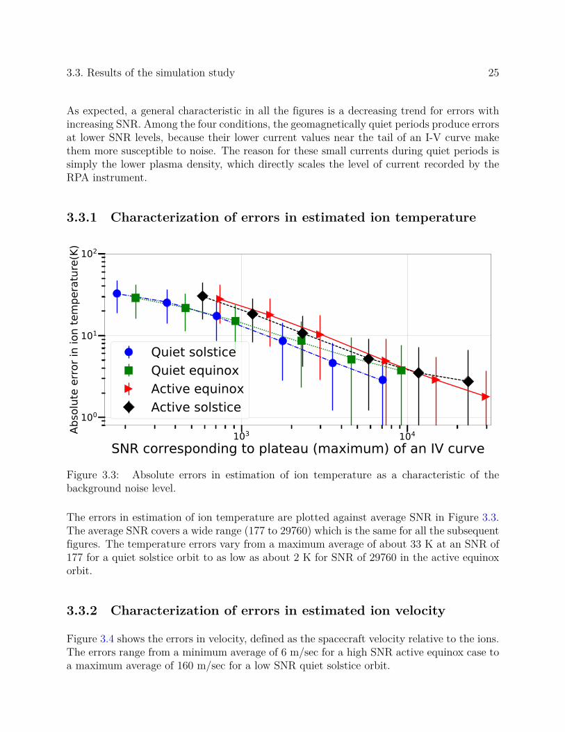
As expected, a general characteristic in all the figures is a decreasing trend for errors withincreasing SNR. Among the four conditions, the geomagnetically quiet periods produce errorsat lower SNR levels, because their lower current values near the tail of an I-V curve makethem more susceptible to noise. The reason for these small currents during quiet periods issimply the lower plasma density, which directly scales the level of current recorded by theRPA instrument.
3.3.1 Characterization of errors in estimated ion temperature
103 104
SNR corresponding to plateau (maximum) of an IV curve
100
101
102
Abso
lute
erro
r in
ion
tem
pera
ture
(K)
Quiet solsticeQuiet equinoxActive equinoxActive solstice
Figure 3.3: Absolute errors in estimation of ion temperature as a characteristic of thebackground noise level.
The errors in estimation of ion temperature are plotted against average SNR in Figure 3.3.The average SNR covers a wide range (177 to 29760) which is the same for all the subsequentfigures. The temperature errors vary from a maximum average of about 33 K at an SNR of177 for a quiet solstice orbit to as low as about 2 K for SNR of 29760 in the active equinoxorbit.
3.3.2 Characterization of errors in estimated ion velocity
Figure 3.4 shows the errors in velocity, defined as the spacecraft velocity relative to the ions.The errors range from a minimum average of 6 m/sec for a high SNR active equinox case toa maximum average of 160 m/sec for a low SNR quiet solstice orbit.

26 Chapter 3. Error quantification for uniform noise
103 104
SNR corresponding to plateau (maximum) of an IV curve
101
102
Abso
lute
erro
r in
ram
vel
ocity
(m/s
ec)
Quiet solsticeQuiet equinoxActive equinoxActive solstice
Figure 3.4: Absolute errors in estimation of ram velocity as a characteristic of the back-ground noise level.
3.3.3 Characterization of errors in estimated spacecraft potential
103 104
SNR corresponding to plateau (maximum) of an IV curve
10 2
10 1
Abso
lute
erro
r in
spac
ecra
ft po
tent
ial(V
)
Quiet solsticeQuiet equinoxActive equinoxActive solstice
Figure 3.5: Absolute errors in estimation of spacecraft potential as a characteristic of thebackground noise level.

3.3. Results of the simulation study 27
The term spacecraft charging refers to the modification of the relative potential between thespacecraft amid the ambient plasma Zuccaro and Holt [58]. Charging can result from photo-electron emission, thermal ion and electron flux, energetic particles and similar phenomena.When charging occurs, the retarding voltage seen by the incoming ions is no longer equalto the retarding grid voltages defined by the sweep. In such cases the IV curve is shifted tothe right for negative spacecraft potential relative to the plasma, and to the left for positivepotentials. In this study the spacecraft potentials were simulated to vary arbitrarily in arange of -3.5 V to 0.5 V for each I-V curve, corresponding to reasonable charging levels thatcan occur in mid-inclination LEO. Figure 3.5 shows that the corresponding average errorsvary from 8 mV to a maximum of 0.2 V error in spacecraft potential from I-V curve fits.
3.3.4 Characterization of errors in composition of oxygen ions
103 104
SNR corresponding to plateau (maximum) of an IV curve10 2
10 1
Abso
lute
erro
r in
O+
com
posit
ion(
%)
Quiet solsticeQuiet equinoxActive equinoxActive solstice
Figure 3.6: Absolute errors in estimation of percentage O+ composition as a characteristicof the background noise level.
The estimation of oxygen ion composition is quite accurate as seen in Figure 3.6. Theabsolute error in estimation of percentage composition is plotted along the y-axis. We seethat the maximum average error in O+ percentage composition for any of the orbits is as lowas 0.20% while the minimum is 0.02%. The lowest average error is observed for the highestSNR in the active solstice orbit, while the maximum average error is observed for the quietsolstice orbit corresponding to the lowest SNR.

28 Chapter 3. Error quantification for uniform noise
3.3.5 Characterization of errors in combined composition of molec-ular ion species
103 104
SNR corresponding to plateau (maximum) of an IV curve
10 2
10 1
Abso
lute
erro
r in
high
mas
s com
posit
ion
(%)
Quiet solsticeQuiet equinoxActive equinoxActive solstice
Figure 3.7: Absolute errors in estimation of combined percentage composition of O+2 and
NO+ as a characteristic of the background noise level.
O+ is the dominant ion in all table mid-latitude low Earth orbits. We characterize thehigher mass molecular ion constituents O+
2 and NO+ as a combined species, since the RPAtechnique does not have the resolution required to distinguish between them. Combining theindividual percentage compositions is a commonly adopted method for reporting molecularconstituents. Figure 3.7 shows the error profile in the composition for this combined speciesas a function of SNR. Since the analysis typically yields a fairly accurate estimation of thepercentage of O+, the combined percentage of O+
2 and NO+ is less error prone as well. Themaximum and minimum error in composition percentage are 0.16% and 0.01% respectively,and like the other parameters, the errors decrease with increasing SNR.
3.3.6 Characterization of errors in estimated ion density
The absolute error in overall ion density ranges from an average maximum of 7.34×10⁹ m−3
to an average minimum of 3.96× 10⁸ m−3 with increasing SNR. Density measurements scaledirectly proportional to the aperture size and grid transparency, as mentioned in Section3.2.1. Since the overall plasma density is simply scaled from the plateau region current, weexpect a linear trend in error versus noise level. For our cubesat-sized RPA the percentageerror in number density versus SNR is shown in Figure 3.8. The maximum average percentage
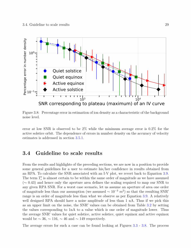
3.4. Guideline to scale results 29
103 104
SNR corresponding to plateau (maximum) of an IV curve
10 1
100
Perc
enta
ge e
rror i
n nu
mbe
r den
sity
Quiet solsticeQuiet equinoxActive equinoxActive solstice
Figure 3.8: Percentage error in estimation of ion density as a characteristic of the backgroundnoise level.
error at low SNR is observed to be 2% while the minimum average error is 0.2% for theactive solstice orbit. The dependence of errors in number density on the accuracy of velocityestimates is addressed in section 3.5.1.
3.4 Guideline to scale results
From the results and highlights of the preceding sections, we are now in a position to providesome general guidelines for a user to estimate his/her confidence in results obtained froman RPA. To calculate the SNR associated with an I-V plot, we revert back to Equation 3.9.The term T ′
r is almost certain to be within the same order of magnitude as we have assumed(∼ 0.43) and hence only the aperture area defines the scaling required to map our SNR toany given RPA SNR. For a worst case scenario, let us assume an aperture of area one orderof magnitude less than our assumption (we assumed ∼ 10−3 m2) so that the resulting SNR′
range is an order of magnitude less than what we observe as per Equation 3.9. A relativelywell designed RPA should have a noise amplitude of less than 1 nA. Thus if we pick thisas an upper limit on the noise, the SNR′ values can be obtained from Table 3.2 by settingthe values corresponding to 1nA to a value which is one order of magnitude lower. Thusthe average SNR′ values for quiet solstice, active solstice, quiet equinox and active equinoxwould be ∼ 36, ∼ 116, ∼ 46 and ∼ 149 respectively.
The average errors for such a case can be found looking at Figures 3.3 - 3.8. The process
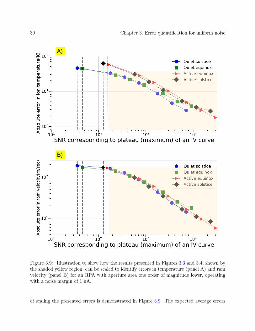
30 Chapter 3. Error quantification for uniform noise
B)
A)
Figure 3.9: Illustration to show how the results presented in Figures 3.3 and 3.4, shown bythe shaded yellow region, can be scaled to identify errors in temperature (panel A) and ramvelocity (panel B) for an RPA with aperture area one order of magnitude lower, operatingwith a noise margin of 1 nA.
of scaling the presented errors is demonstrated in Figure 3.9. The expected average errors
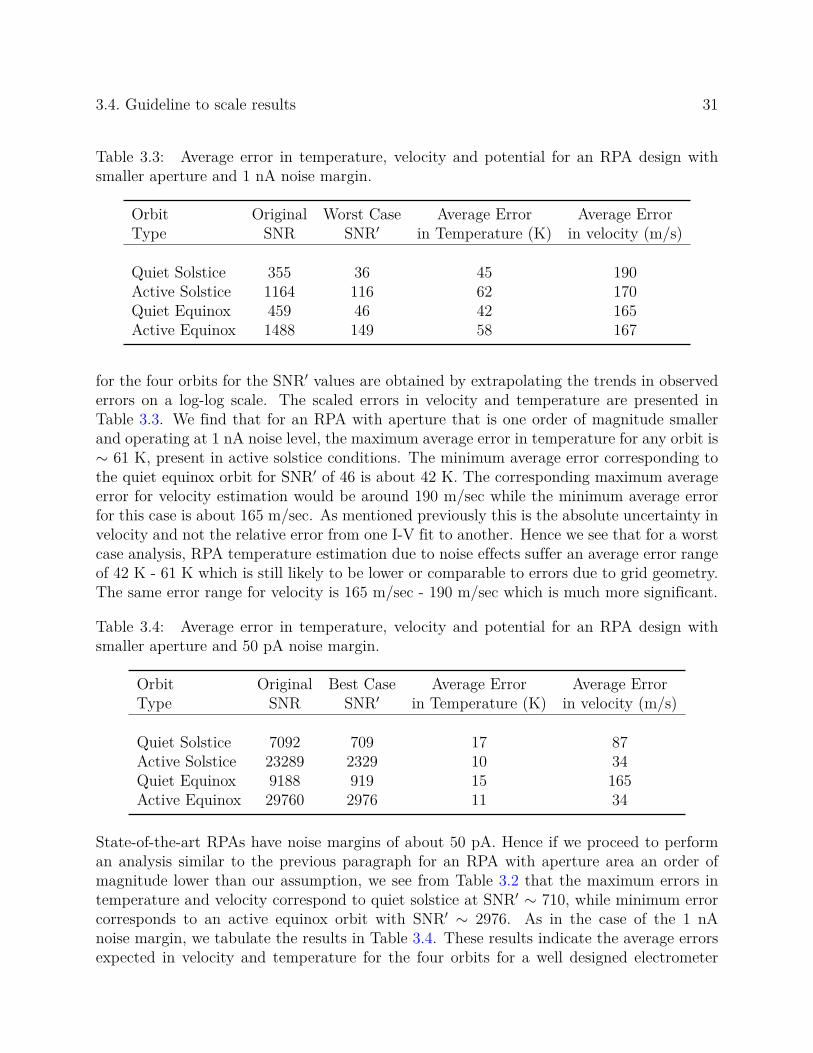
3.4. Guideline to scale results 31
Table 3.3: Average error in temperature, velocity and potential for an RPA design withsmaller aperture and 1 nA noise margin.
Orbit Original Worst Case Average Error Average ErrorType SNR SNR′ in Temperature (K) in velocity (m/s)
Quiet Solstice 355 36 45 190Active Solstice 1164 116 62 170Quiet Equinox 459 46 42 165Active Equinox 1488 149 58 167
for the four orbits for the SNR′ values are obtained by extrapolating the trends in observederrors on a log-log scale. The scaled errors in velocity and temperature are presented inTable 3.3. We find that for an RPA with aperture that is one order of magnitude smallerand operating at 1 nA noise level, the maximum average error in temperature for any orbit is∼ 61 K, present in active solstice conditions. The minimum average error corresponding tothe quiet equinox orbit for SNR′ of 46 is about 42 K. The corresponding maximum averageerror for velocity estimation would be around 190 m/sec while the minimum average errorfor this case is about 165 m/sec. As mentioned previously this is the absolute uncertainty invelocity and not the relative error from one I-V fit to another. Hence we see that for a worstcase analysis, RPA temperature estimation due to noise effects suffer an average error rangeof 42 K - 61 K which is still likely to be lower or comparable to errors due to grid geometry.The same error range for velocity is 165 m/sec - 190 m/sec which is much more significant.
Table 3.4: Average error in temperature, velocity and potential for an RPA design withsmaller aperture and 50 pA noise margin.
Orbit Original Best Case Average Error Average ErrorType SNR SNR′ in Temperature (K) in velocity (m/s)
Quiet Solstice 7092 709 17 87Active Solstice 23289 2329 10 34Quiet Equinox 9188 919 15 165Active Equinox 29760 2976 11 34
State-of-the-art RPAs have noise margins of about 50 pA. Hence if we proceed to performan analysis similar to the previous paragraph for an RPA with aperture area an order ofmagnitude lower than our assumption, we see from Table 3.2 that the maximum errors intemperature and velocity correspond to quiet solstice at SNR′ ∼ 710, while minimum errorcorresponds to an active equinox orbit with SNR′ ∼ 2976. As in the case of the 1 nAnoise margin, we tabulate the results in Table 3.4. These results indicate the average errorsexpected in velocity and temperature for the four orbits for a well designed electrometer
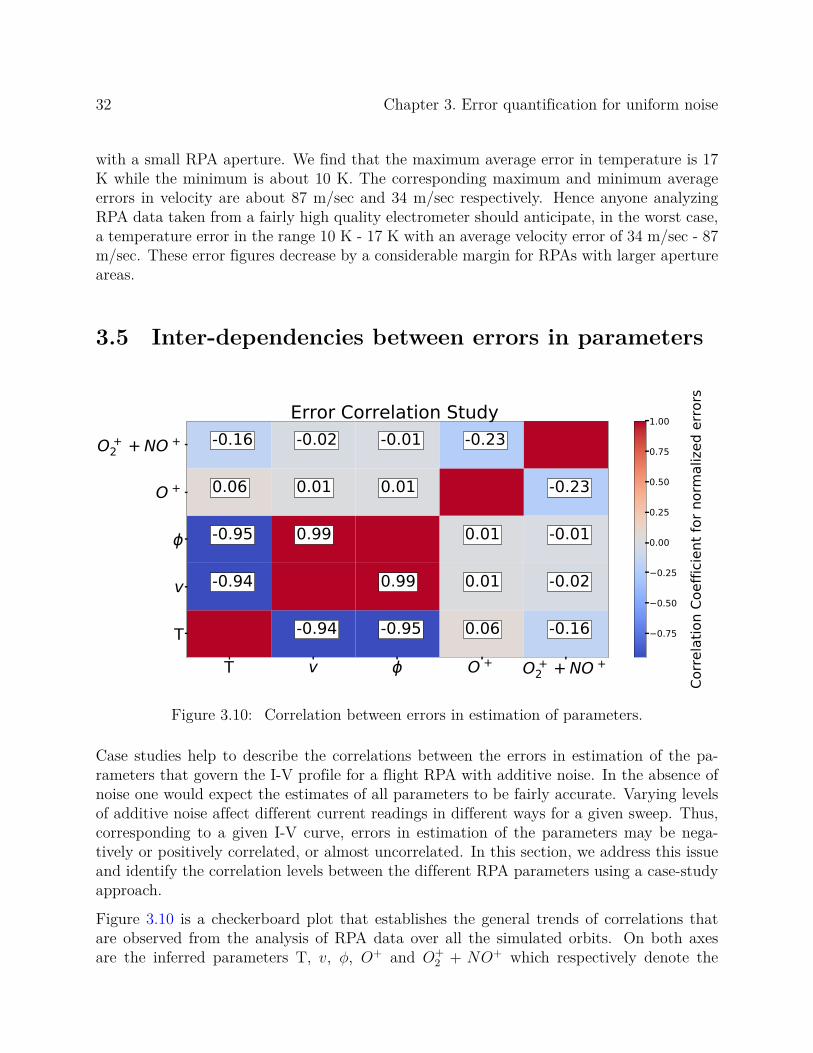
32 Chapter 3. Error quantification for uniform noise
with a small RPA aperture. We find that the maximum average error in temperature is 17K while the minimum is about 10 K. The corresponding maximum and minimum averageerrors in velocity are about 87 m/sec and 34 m/sec respectively. Hence anyone analyzingRPA data taken from a fairly high quality electrometer should anticipate, in the worst case,a temperature error in the range 10 K - 17 K with an average velocity error of 34 m/sec - 87m/sec. These error figures decrease by a considerable margin for RPAs with larger apertureareas.
3.5 Inter-dependencies between errors in parameters
T v O + O +2 + NO +
T
v
O +
O +2 + NO +
-0.94 -0.95 0.06 -0.16
-0.94 0.99 0.01 -0.02
-0.95 0.99 0.01 -0.01
0.06 0.01 0.01 -0.23
-0.16 -0.02 -0.01 -0.23Error Correlation Study
0.75
0.50
0.25
0.00
0.25
0.50
0.75
1.00
Corre
latio
n Co
effic
ient
for n
orm
alize
d er
rors
Figure 3.10: Correlation between errors in estimation of parameters.
Case studies help to describe the correlations between the errors in estimation of the pa-rameters that govern the I-V profile for a flight RPA with additive noise. In the absence ofnoise one would expect the estimates of all parameters to be fairly accurate. Varying levelsof additive noise affect different current readings in different ways for a given sweep. Thus,corresponding to a given I-V curve, errors in estimation of the parameters may be nega-tively or positively correlated, or almost uncorrelated. In this section, we address this issueand identify the correlation levels between the different RPA parameters using a case-studyapproach.
Figure 3.10 is a checkerboard plot that establishes the general trends of correlations thatare observed from the analysis of RPA data over all the simulated orbits. On both axesare the inferred parameters T, v, ϕ, O+ and O+
2 + NO+ which respectively denote the
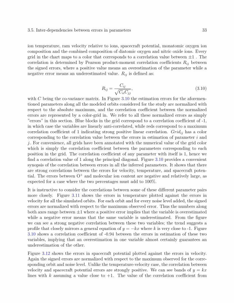
3.5. Inter-dependencies between errors in parameters 33
ion temperature, ram velocity relative to ions, spacecraft potential, monatomic oxygen ioncomposition and the combined composition of diatomic oxygen and nitric oxide ions. Everygrid in the chart maps to a color that corresponds to a correlation value between ±1 . Thecorrelation is determined by Pearson product-moment correlation coefficients Rij betweenthe signed errors, where a positive value means an overestimation of the parameter while anegative error means an underestimated value. Rij is defined as:
Rij =Cij√CiiCjj
, (3.10)
with C being the co-variance matrix. In Figure 3.10 the estimation errors for the aforemen-tioned parameters along all the modeled orbits considered for the study are normalized withrespect to the absolute maximum, and the correlation coefficient between the normalizederrors are represented by a color-grid in. We refer to all these normalized errors as simply”errors” in this section. Blue blocks in the grid correspond to a correlation coefficient of -1,in which case the variables are linearly anti-correlated, while reds correspond to a maximumcorrelation coefficient of 1 indicating strong positive linear correlation. Gridij has a colorcorresponding to the correlation value between the errors in estimation of parameter i andj. For convenience, all grids have been annotated with the numerical value of the grid colorwhich is simply the correlation coefficient between the parameters corresponding to eachposition in the grid. The correlation coefficient of any parameter with itself is 1, hence wefind a correlation value of 1 along the principal diagonal. Figure 3.10 provides a convenientsynopsis of the correlation between errors in all the inferred parameters. It shows that thereare strong correlations between the errors for velocity, temperature, and spacecraft poten-tial. The errors between O+ and molecular ion content are negative and relatively large, asexpected for a case where the two percentages must add to 100%.
It is instructive to consider the correlations between some of these different parameter pairsmore closely. Figure 3.11 shows the errors in temperature plotted against the errors invelocity for all the simulated orbits. For each orbit and for every noise level added, the signederrors are normalized with respect to the maximum observed error. Thus the numbers alongboth axes range between ±1 where a positive error implies that the variable is overestimatedwhile a negative error means that the same variable is underestimated. From the figurewe can see a strong negative correlation between these two variables; the trend suggests aprofile that closely mirrors a general equation of y = −kx where k is very close to -1. Figure3.10 shows a correlation coefficient of -0.94 between the errors in estimation of these twovariables, implying that an overestimation in one variable almost certainly guarantees anunderestimation of the other.
Figure 3.12 shows the errors in spacecraft potential plotted against the errors in velocity.Again the signed errors are normalized with respect to the maximum observed for the corre-sponding orbit and noise level. Unlike the temperature-velocity case, the correlation betweenvelocity and spacecraft potential errors are strongly positive. We can see bands of y = kxlines with k assuming a value close to +1. The value of the correlation coefficient from
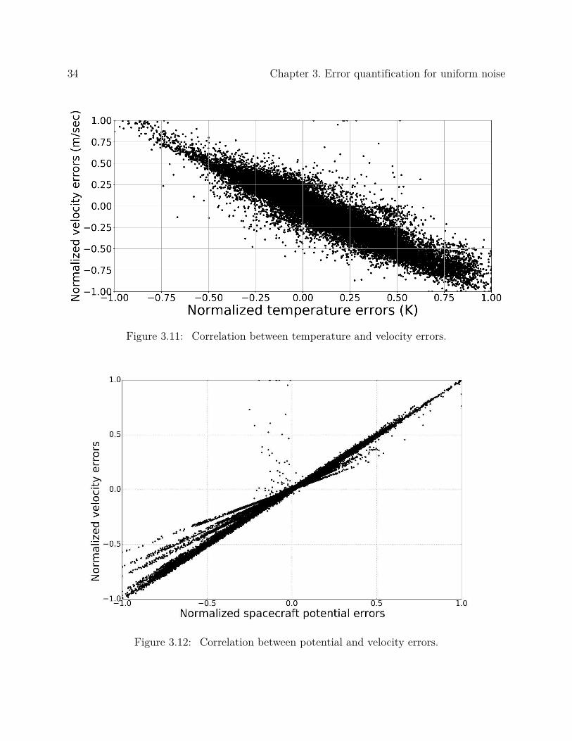
34 Chapter 3. Error quantification for uniform noise
Figure 3.11: Correlation between temperature and velocity errors.
Figure 3.12: Correlation between potential and velocity errors.

3.5. Inter-dependencies between errors in parameters 35
Figure 3.10 is 0.99. The deviation in spacecraft potential increases as the uncertainty in thevelocity increases.
Figure 3.13: Correlation between O+ composition and velocity errors.
The value of the correlation coefficient between O+ percentage composition errors and ve-locity errors as seen in Figure 3.10 is 0.02. This suggests that the two variables are largelyuncorrelated and this borne out by the scatter plot shown in Figure 3.13. A lack of corre-lation ensures that the errors in one variable are largely independent (linearly independent)of the corresponding errors in the other variable. Figure 3.13 shows three clusters of data,each of which individually portray an uncorrelated trend. The three most apparent clus-ters align parallel to the y-axis i.e. x = k1 (k1 being a constant) with the center cluster(clustered around x = k1 ≈ 0) being most prominent. There is also a thin band of pointsthat align almost along the x-axis i.e., y ≈ 0. Such parallel bands along the axes reflect thefact that one cannot predict how the composition estimates would deviate given a deviationin the velocity estimate. Since we have already established that errors in potential and ve-locity (positive) and velocity and temperature (negative) show strong correlation, it can beinferred that the composition errors are relatively uncorrelated behavior with any of thesethree parameter errors (temperature, velocity, potential). This is also substantiated throughFigure 3.10 where the correlation values for T-O+,v-O+ and ϕ-O+ are 0.06, 0.02 and 0.01,respectively.
36 Chapter 3. Error quantification for uniform noise
3.5.1 A discussion on the estimation of density errors
Density errors have intentionally been omitted from the case-study. Density is the parameterthat primarily determines the peak level of the I-V curve. Inferences about other parame-ters are determined after normalizing the I-V curves so that the dependence on density isremoved. However, the peak level also is affected by the ion speed in the direction normalto the aperture. Thus the variable that determines the peak of an I-V curve is the productof density and velocity as evident in equation (3.7). As a result the velocity error marginstypically mirror the density error margins but are opposite in sign (strong negative correla-tion). Indeed the correlation coefficient observed is -0.96. Since velocity and potential arepositively correlated while temperature and velocity are negatively correlated, the negativecorrelation applies to density and potential errors (-0.96), while temperature is expected toshow strong positive correlation (0.92). It is interesting to note that correlation of densityerrors with temperature or potential does not imply dependence between these parameters,since it is evident that density estimation depends only on velocity and all other correlationsare a byproduct of this dependence.
3.6 Orbit coverage of simulation study
The simulation I-V curves presented in this chapter were generated using empirical valuesof temperatures, densities and composition for equinox and solstice in quiet and active con-ditions for a mid-inclination orbit at altitudes where molecular ions are present. However,for the sake of brevity and feasibility, we limited the scope of the study to a specific timerange. By choosing a specific orbit we unintentionally incorporate some degree of bias inour simulations, and hence in any general conclusions we make. To understand the extentof this bias, we have performed a validation study that quantifies the range of geophysicalinput parameter values for our chosen orbit versus other orbits. Figure 3.14 shows threepanels for three input parameters: ion temperature, ion number density and percentage ofmolecular ions. Each panel consists of two box-plots - one for the single orbit case used inour study and the other for a more comprehensive set of ”validation orbits”. These orbitsare obtained by choosing four different local times at the south-north equatorial crossing.These local-times are phased at 6-hour intervals to span one complete day, and each of thesefour orbits are simulated using the IRI empirical model for solar and seasonal variations asperformed in the original study. These validation orbits show that the orbit phase effects onthe parameter values are small, so our test orbit has not introduced any biases or limitationson the parameter ranges studied. The comparisons with the single orbit case are shown inFigure 3.14. Each pair of box-plots in each panel in the figure shows the interquartile rangedemarcated by the limiting ends of the box. The vertical dotted line inside each box ismedian, and the solid line is the mean. The entire range of values are shown by end pointsof the whiskers extending from the box-plots on either end.
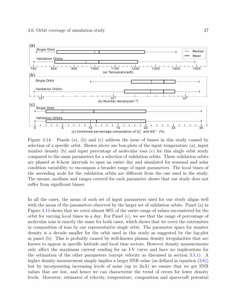
3.6. Orbit coverage of simulation study 37
700 800 900 1000 1100 1200 1300 1400 1500(a) Tem perature(K)
Single Orbit
Validat ion Orbits
(a)
Median
Mean
104
105
106
(b) Num ber density(cm 3)
Single Orbit
Validat ion Orbits
(b)
0 5 10 15 20 25 30
(c) Com bined percentage com posit ion of O +2 and NO + (%)
Single Orbit
Validat ion Orbits
(c)
Figure 3.14: Panels (a), (b) and (c) address the issue of biases in this study caused byselection of a specific orbit. Shown above are box-plots of the input temperature (a), inputnumber density (b) and input percentage of molecular ions (c) for this single orbit studycompared to the same parameters for a selection of validation orbits. These validation orbitsare phased at 6-hour intervals to span an entire day and simulated for seasonal and solarcondition variability to encompass a broader range of input parameters. The local times ofthe ascending node for the validation orbits are different from the one used in the study.The means, medians and ranges covered for each parameter shows that our study does notsuffer from significant biases.
In all the cases, the mean of each set of input parameters used for our study aligns wellwith the mean of the parameters observed by the larger set of validation orbits. Panel (a) inFigure 3.14 shows that we cover almost 90% of the entire range of values encountered for theorbit for varying local times in a day. For Panel (c), we see that the range of percentage ofmolecular ions is exactly the same for both cases, which shows that we cover the extremitiesin composition of ions by our representative single orbit. The parameter space for numberdensity is a decade smaller for the orbit used in this study as suggested by the log-plotin panel (b). This is probably caused by well-known plasma density irregularities that areknown to appear in specific latitude and local time sectors. However density measurementsonly affect the maximum current reading for an I-V curve and have no implications forthe estimation of the other parameters (except velocity as discussed in section 3.5.1). Ahigher density measurement simply implies a larger SNR value (as defined in equation (3.6))but by incorporating increasing levels of noise (up to 2nA) we ensure that we get SNRvalues that are low, and hence we can characterize the trend of errors for lower densitylevels. Moreover, estimates of velocity, temperature, composition and spacecraft potential
38 Chapter 3. Error quantification for uniform noise
are obtained from normalized I-V curves which implies that input density does not affectthese estimates except by changing the SNR. The input parameter profiles for ram velocityand spacecraft potential have been intentionally left out of the figure since these parameterswere uniformly distributed for this study within practical ranges. Velocity varies uniformlybetween 7.5 km/sec and 8.2 km/sec for this study while the range for spacecraft potential is-3.5 V to 0.5 V.
Chapter 4
Dissecting the problem: Analyticalstudy of I-V curves
4.1 Why we need an analytical investigation
Prior to further investigating RPA analysis approaches computationally it is instructive todevelop an analytical understanding. We begin with re-iterating the I-V characteristic of anRPA in terms of the associated physical parameters as presented by Knudsen [38]:
I = TrAev cos θ∑i
ni[1
2+
1
2erf(κi) +
exp(−κ2i )
2(π)12αi
], (4.1)
whereκi = ai − b. (4.2)
ai = v cos θ/αi. (4.3)
αi = (2kT/mi)12 . (4.4)
b = (e(x+ ϕ)/kT )12 . (4.5)
Equation (4.1) shows the current profile for a sweeping range x of retarding voltages, summedover the number of ion species. The variables v, T and ϕ correspond to the spacecraft velocityrelative to the ions, the ion temperature and the spacecraft potential, respectively. The ni
variable is the number density of the i-th species of ion. Since∑
ni equals the total iondensity n, it can be moved outside the summation and the resulting sum can be shown tovary from 0 to 1 depending on the retarding potential x. The remaining parameters Tr , Aand θ are respectively the transparency of the grids, the aperture area and the angle at whichthe normal vector of the aperture is tilted from the direction of spacecraft motion relativeto the ions. These factors define the geometry of the RPA instrument and only contributeto the scaling of the normalized current profile.
In practice the measured I-V characteristics are processed using a multi-dimensional curvefitting analysis to infer the parameters v, ϕ and T , which (along with ni) are the physicalvariables of interest. It should be noted that the velocity v inferred from the fit is the ionvelocity relative to the spacecraft, which moves at orbital velocity (∼ 8 km/s). The bulk
39

40 Chapter 4. Dissecting the problem: Analytical study of I-V curves
ion velocity in the Earth frame is typically much less than the orbital satellite speed so theions entering the RPA aperture are supersonic. It is important to remind the readers of theimplicit assumptions present in the I-V analysis approach. First, it is assumed that noneof the parameters change significantly over the time required to sweep the voltage of theretarding grid over its full range. Second, the different ion species collected by the RPA areall in thermodynamic equilibrium and described by the same temperature T .
Low energy plateau
Transition Region High energy tail
Figure 4.1: Different sections of a normalized I-V curve.
Figure 4.1 shows an idealized graph of the I-V curve for a single ion species. When normal-ized by the maximum value attained (at zero retarding voltage), the I-V characteristic isindependent of the ion density and can be studied to investigate the relationships betweentemperature, velocity and potential. Debchoudhury and Earle [16] show a strong positivelinear correlation between the errors in velocity and potential in the presence of noise. Herewe investigate this further to study the extent of cross-linking between these two parameters.
The work by Klenzing et al. [36] discusses the most important factors that introduce noiseinto the measured I-V curves. Some of these are simply electronic noise that scales as thetemperature of the electronics, but others are related to small distortions in the particledistributions introduced by their passage through the grid system. All of these effects canbe considered as sources of noise for the present study. While there may not be any obviousphysical rationale that addresses why velocity and potential estimation errors are stronglyinter-linked in the presence of noise, it is worth noting that for a Maxwellian distribution,both of these energy-related parameters manifest themselves in the same way in the I-Vprofile, as shown in the expressions for ai and b in equations (4.2) through (4.5). The leakageand lensing effects described by Klenzing et al. [36] and Davidson et al. [13] introduce small
4.2. Analytical relation between errors in velocity and potential 41
distortions that are compounded by electronic noise. As a result, it can be extremely difficultto isolate the individual impacts of velocity and potential in a noisy I-V curve.
In order to understand how a curve fitting algorithm impacts the estimation of potentialand velocity, we shall attempt to analytically derive conditions under which the I-V profilescan be approximately similar for dissimilar values of velocity and potential. The procedureis illustrated in the subsequent section.
4.2 Analytical relation between errors in velocity andpotential
Let us assume that at a certain temperature T and retarding voltage x, a velocity-potentialpair (v, ϕ) generates a normalized current value that is similar to that from a referencevelocity-potential pair (vref , ϕref ) at the same temperature. It should be noted that ”similar”means that the difference between the two current values lies within the envelope of the noisestandard deviation, so that both values are essentially viable solutions to the model fit whennoise is present. Let these two sets of parameter combinations (T, v, ϕ) and (T, vref , ϕref ) berelated to κ and κref respectively, through equation (4.2). According to (4.1) - (4.5) whenκ = κref , the current values are equal at retarding voltage x (the exponential term is muchsmaller in general than the error function term, and only varies with velocity and kappa forthe same temperature). The following analytical treatment is aimed at finding v and ϕ forgiven vref and ϕref that generate I-V profiles that are approximately similar. For constante, θ and Tr, and defining A =
√m2k
, B =√
ek, ∆ϕ = ϕ−ϕref , ∆v = v− vref , we set κ = κref
and use equations (4.2) - (4.5) to obtain:
Av√T
−B
√x+ ϕ
T=
Avref√T
−B
√x+ ϕref
T. (4.6)
=⇒ A∆v = B(√x+ ϕ−
√x+ ϕref ). (4.7)
In order to progress further we define the different sections of a typical single-species I-Vcurve. Figure 4.1 shows a normalized I-V curve with different regions of interest labeled. TheI-V curve for supersonic orbital velocities results from the integration of the first momentof the Maxwellian distribution with appropriate limits. The transition region in Figure 4.1defines the shape of the Maxwellian from which it was generated and is the region mostsensitive to the parameters defining the I-V profile. For spacecraft potentials and velocitiesthat are expected in a quiescent F-region ionosphere, we can justifiably assume that thetransition region is within a range of retarding voltages that are large compared to thespacecraft potential. A Taylor series expansion of equation (10) up to 3 terms leads to:

42 Chapter 4. Dissecting the problem: Analytical study of I-V curves
A∆v = B√x(
√1 +
ϕ
x−
√1 +
ϕref
x). (4.8)
A∆v ≈ B√x(
ϕ− ϕref
2x−
ϕ2 − ϕ2ref
8x2). (4.9)
The normalized current is unity at x=0, and so we can divide by x for all non-zero retardingvoltages. Now we can approximate, using ∆ϕ = ϕ− ϕref :
A
B∆v ≈
√x(
∆ϕ
2x− 1
4x2ϕref∆ϕ(
∆ϕ
2ϕref
+ 1)). (4.10)
For cases when (∆ϕ) << ϕref , that is for some range of ϕ near ϕref , we obtain the analyticalrelation
∆v
∆ϕ≈ B
A(
1
2√x− ϕref
4x√x), (4.11)
which can be now written using definitions of ∆v and ∆ϕ as:
v ≈ [B
A(
1
2√x− ϕref
4x√x)](ϕ− ϕref ) + vref , (4.12)
and
ϕ ≈ [A
B( 12√x− ϕref
4x√x)](v − vref ) + ϕref . (4.13)
If (vref , ϕref ) is the accurate parameter combination corresponding to a reference noise-freeI-V profile then equations (4.12) and (4.13) help generate (v, ϕ) combinations that yieldnormalized I-V curves that are approximately similar to the reference I-V profile under as-sumptions specified. If the degree of difference between the I-Vs generated by the referencevelocity-potential pair and the approximately similar I-V generated by these equations iscomparable to or less than the degree of noise present in the measurement, then it is impos-sible for a fitting algorithm to choose between these profiles.
To illustrate this point, we select a reference velocity-potential pair of (7800 m/s, -0.5 V).We choose a temperature of 600 K and an ion density of 104 cm−3 in the presence of only O+
species. We choose calculate using equation (4.12), corresponding velocity values that wouldyield normalized I-V curves similar to the one obtained from this reference pair for potentialvalues ϕ = −0.375 V and ϕ = −0.625 V. The assumption that |∆ϕ| << |ϕref | is met andthus we obtain the two velocity values as v = 7898 m/s and v = 7702 m/s. We plot the noisefree I-V curves corresponding to the reference pair and also for the two obtained pairs (-0.375

4.2. Analytical relation between errors in velocity and potential 43
Difference~ 100 pA
Figure 4.2: The picture shows the validity of the analytically obtained relation in (4.11).The envelope denotes the potential-velocity combinations that yield a normalized I-V curvethat lie within one noise standard deviation of a curve generated by an ideal referencevelocity-potential pair. The line denotes the analytical relation outlined in (4.11) for thesame reference pair. The colorbar denotes the variation of Euclidean distance from the idealreference I-V curve for all the pairs that generates I-V curves within the noise envelope.
V, 7898 m/s) and (-0.625 V, 7702 m/s). These are shown in Figure 4.2 in black, red andblue respectively. The I-V curves are not normalized and scaled for the geometry presentedin the study in Chapter 3. A section of the transition region is zoomed in and it is seen thatthe difference between the current measurements between the reference profile and each ofthe two obtained profiles are of the order of 100 pA. Even for realistic well-designed RPAs,a noise level of 100 pA is common, and thus it can be stated that in presence of noise, eitherof the red or the blue profile ( which differs in velocity by about 100 m/s) can be obtainedas a solution in place of the black desired profile. This shows that the analytical relationderived indeed serves to identify velocity potential pairs yielding approximately similar I-Vprofiles. The similarity increases as ∆ϕ decreases. Also, the shown similarity profiles aretwo out of many possible , and the spectrum of such velocity-potential pairs increase withdecreasing signal-to-noise ratio.
It is thus apparent that the analysis of a single noisy I-V profile can have infinitely manycombinations of velocity-potential pairs as outcomes of an estimation algorithm. This isof particular significance since it provides insight into the inherent challenges of the noisyRPA data analysis algorithm. For any realistic noise level, it is impossible for any estimationalgorithm to label a certain velocity-potential combination as a unique and accurate solution.Furthermore, since the curve fitting analysis is performed iteratively starting with someinitialization, it is impossible to guarantee that the final values inferred for the parametersof interest are the ”best fit”. In other words, the minimum mean squared error fitting routine

44 Chapter 4. Dissecting the problem: Analytical study of I-V curves
may converge to different but equally valid solutions depending on the initial estimates used.
4.3 Validating the analytical relation
To test the validity of the point made in section 4.2, we choose the same reference pair asin Figure 4.2 and calculate all the combinations in a velocity-potential space that generatesuch similar curves from realistic noise calculated from the noise distribution presented insection 2.3. The result is shown in Figure 4.3, where the solid black line spans combinationsthat satisfy the analytically obtained relationship given by equation (4.12) for the chosenreference potential-velocity pair. Note that all other parameters are kept constant so thatwe can solely study the interdependence between velocity and potential errors. We addnoise corresponding to an operating temperature of 25◦ C to an ideal I-V curve generatedfor the reference combination according to equation (2.4), and then find the combinationsthat yield I-V curves lying within one noise standard deviation of the reference I-V curve.These combinations of velocity and potential are all plotted in the scatter plot with bluesrepresenting points closest to the reference combination and reds representing those farthestaway, yet within the same one standard deviation bound. The figure indicates that theanalytical relation is a decent representation of the velocity-potential pairs that are equallylikely candidates as estimates to the reference noise-free pair. The goodness of fit degradesas we move further along the potential axis from the reference potential (-0.5 V) as theapproximation of (∆ϕ) << ϕ2 becomes increasingly invalid. An interesting observationfrom the figure is that the plausible velocity potential pairs encompass a wide range in bothvelocity (more than 500 m/s) and potential (more than 0.7 V ) space, and this is detrimentalto the analysis process. In the presence of any noise, a primitive fitting algorithm cannotdistinguish the best solution from among all the candidate solutions. Instead it will convergeto estimates of velocity and potential that depends on the initial guess, the step size andother fitting parameters. Large errors can result from this process.
Thus Figure 4.3 is an experimental validation of the analytical relation (4.12). The argumentsabove establish that analysis of an I-V curve with added noise can yield several equally likelysolutions that are similar in terms of the sum of squared errors but very different in termsof the parameter values. Two noise samples from the same noise distribution can generateI-V curves which, when subjected to a curve-fit algorithm minimizing for least squares fit,can yield solutions that are different but equally valid. To improve the analysis, we need animproved algorithm for RPA curve fitting that differs from the methods currently used byexperimental space scientists.

4.4. The noise effect from an algorithm perspective 45
Figure 4.3: The picture shows the validity of the analytically obtained relation in (4.11). Theenvelope denotes the potential-velocity combinations that yield normalized I-V curves thatlie within one noise standard deviation of a curve generated by an ideal reference velocity-potential pair at 25◦ C . The black line denotes the analytical relation outlined in (4.12) forthe same reference pair for the entire potential range. The colorbar denotes the variationof Euclidean distance from the ideal reference I-V curve for all the pairs that generate I-Vcurves within the noise envelope.
4.4 The noise effect from an algorithm perspective
In the previous section we demonstrated how multiple solutions can lie within one noisestandard deviation of the global optimum. The analytical relation presented generates thesesolutions within valid approximations. Next we take a step back and try to visualize thenoise problem from an algorithm perspective. After all, what a fitting algorithm actuallytries to achieve is to intelligently generate solutions that yield an I-V curve that is ’closest’ tothe measured I-V curve one is fitting. ’Closest’ is essentially a qualitative way of describingthe objective function - the quantitative cost function that is evaluated at every iterationof the I-V fitting procedure. In most typical cases, the cost function is simply the sum ofthe squared errors (sse) between the solution generated and the measured I-V curve. Thecombination that yields the minimum sse is the solution.
The entire noise problem is essentially a study of how noise affects the sse between a rep-resentative noisy I-V curve and the candidate I-V curves generated from the admissiblesolution space. In order to understand this in greater detail we plot the sse contours for
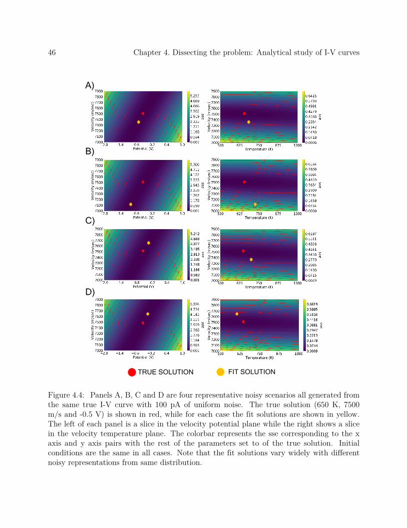
46 Chapter 4. Dissecting the problem: Analytical study of I-V curves
TRUE SOLUTION FIT SOLUTION
B)
A)
C)
D)
Figure 4.4: Panels A, B, C and D are four representative noisy scenarios all generated fromthe same true I-V curve with 100 pA of uniform noise. The true solution (650 K, 7500m/s and -0.5 V) is shown in red, while for each case the fit solutions are shown in yellow.The left of each panel is a slice in the velocity potential plane while the right shows a slicein the velocity temperature plane. The colorbar represents the sse corresponding to the xaxis and y axis pairs with the rest of the parameters set to of the true solution. Initialconditions are the same in all cases. Note that the fit solutions vary widely with differentnoisy representations from same distribution.

4.4. The noise effect from an algorithm perspective 47
pairs of parameter combinations. In Figure 4.4 these plots are shown in four panels. Theleft columns are plots in the potential-velocity space while the right panels describe thetemperature-velocity space. For all these plots a parameter combination is chosen as thedesired solution and indicated by the red dots in Figure 4.4. Also, the initial seeds are samefor each case. The noise-free I-V curve is calculated from equations (4.1) - (4.5). Four noisyrepresentations of this idealized I-V curve, represented by the four panels in the figure, arecalculated by drawing from a uniform noise distribution centered on 100 pA of noise. Thesefour I-V curves are analyzed with a Levenberg-Marquardt curve-fitting scheme, and the fitsolutions are shown by the yellow dots. The color at each 2-D grid point represents thesum-squared error between the noise-free I-V and the I-V generated by the combination(velocity-potential for the left column, velocity-temperature for the right column). All otherparameters same as from the true solution. Thus essentially these plots are slices in thecomplete parameter space.
The figure shows that for different noisy representations, even with same initial conditions,the solutions can vary widely. For panels A and B, potential and velocity estimates areunderestimated while temperature is overestimated. For C and D potential and velocity areoverestimated. Temperature is underestimated in D and overestimated in C. The resultsshow that the fit solution is largely dependent not only on the amount of noise (as shownin chapter 3), but also on how the noise is added. This is because of the fact that the I-Vcurve has a number of sensitive regions as labeled in Figure 4.1. The shape of the transitionregion is heavily dependent on the parameters that define the I-V curve. Thus dependingon how noise is added and how the I-V curve is distorted, a fitting algorithm may generatevery different solutions.
It is with the rationale outlined above that we proceed to look for an improved autonomousalgorithm — one that is less dependent on how the noise is added. The patterns of pa-rameter interdependence presented here make a compelling case that not one, but multiplerepresentations of a single noisy I-V curve are necessary for the estimation process. In thefollowing chapter, we explore a new robust algorithm for RPA curve-fitting that improvesthe outcome autonomously.
Chapter 5
BATFORD: An improved algorithm
The previous chapter highlights the uncertainties associated with the analysis of RPA datausing a traditional approach. Indeed one cannot have confidence that the velocity or poten-tial estimated by one run of a traditional iterative Levenberg-Marquardt (LM) algorithm isaccurate enough. Stated differently, the error bars that would be associated with the param-eters inferred from such curve fits would be quite large. The distribution of noise is one ofthe major reasons that degrade the estimation accuracy, particularly when plasma densitiesare low, and thus the process can be improved by using statistical measures to resample thenoisy normalized I-V profile. We implement the resampling procedure through an approachcommonly known as bootstrap in the statistics terminology.
5.1 Bootstrap method for resampling
Bootstrap [17, 18, 20] is a classical and well-studied resampling technique in statistics. In itssimplest form, the idea is to construct resamples by taking samples with replacement from theoriginal dataset, and applying the estimation or inference method on the resamples. Thisis a popular and powerful procedure that can be applied to a wide variety of estimation,prediction, and inference problems. It has great conceptual appeal as it is straightforwardto implement, using resamples from the data itself, and is automatic in nature such that apractitioner does not require advanced statistical know-how to implement the procedure. Re-cent advances in bootstrap methodology include efficient strategies for big data applications[35, 52] and resampling techniques for complex data, e.g., irregularly spaced spatio-temporaldatasets [51, 53].
In order to describe the concept of the bootstrap, let us consider a simple linear model:
yi = a+ bxi + ϵi, (5.1)
where yi is the data point at i-th observation for given input xi. The term ϵi denotes theuncertainty or noise present in the corresponding measurement. For this linear mode, a andb are the parameters that are estimated.
We apply a fitting routine and obtain the least-squares estimates of a and b as a and brespectively. The corresponding best fit y values are given by yi:
yi = a+ bxi. (5.2)
48

5.1. Bootstrap method for resampling 49
The errors in estimation are ϵi which are the estimates for the uncertainty that was presentin the observed data.
ϵi = yi − yi, (5.3)=⇒ ϵi = yi − a− bxi. (5.4)
Now, the concept of bootstrap resampling is to compute new set of residuals ϵ∗i from theestimated residuals ϵi that can now be used to generate a new sample set of observations y∗i .
y∗i = yi + ϵ∗i (5.5)=⇒ y∗i = a+ bxi + ϵ∗i . (5.6)
Here y∗i is another representative sample which is similar in form to yi in equation (5.1). Theresampled data y∗i can now be fitted in a manner similar to yi to obtain new estimates ofthe model parameters a and b. The intricacies in the procedure lie in generating bootstrapsamples ϵi which determines the efficiency of the objective. We now proceed to understandthe bootstrap procedure in the context of this dissertation.
From a statistical perspective, the I-V observations can be interpreted as data generated froma non-linear regression model, with the functional form of the regression model given by (4.1).Of course, we can only observe a noisy version of the data, and our goal is to estimate theparameters of this model from these noisy observations. Our parameter estimation strategyis based on two techniques from the bootstrap toolbox — namely, bootstrap smoothing andwild bootstrap.
Bootstrap smoothing was introduced by Efron and Tibshirani [19] as a form of model av-eraging based on bootstrap resampling. The basic idea is to construct a large number ofbootstrap replicates from a dataset, estimate parameters from each replicate, and take theaverage of the estimated parameters. This strategy is closely related to ensemble learningmethods like bagging [5, 7], where a similar idea is used for prediction, and to random forests[6], where a similar idea is used for feature selection. For the RPA data, we apply boot-strap smoothing by estimating parameters from an ensemble of resampled I-V datasets, andreporting the average of these estimated parameters as our final estimate.
One complicating factor is that, as observed from our investigation in Section 2.3, the noisein the I-V curve is heteroscedastic, i.e., different data points in the I-V curve have differentnoise distributions. Therefore, we cannot resample from the ensemble of model residualsusing sampling without replacement directly, as the model residuals at different data pointsare not exchangeable. To address this, we apply a specific kind of bootstrap technique,known as wild bootstrap [42, 56]. The basic idea of wild bootstrap is to resample the model

50 Chapter 5. BATFORD: An improved algorithm
residuals for each data point individually using a Rademacher distribution [11], instead ofresampling from the ensemble of model residuals. This resampling strategy is robust toheteroscedasticity of model residuals, and is, therefore, appropriate for the RPA data.
Our bootstrap strategy leverages a novel combination of wild bootstrap and bootstrapsmoothing. The algorithm for parameter estimation based on this strategy is describedin the next subsection.
5.2 BATFORD algorithm
The algorithm we propose is BATFORD, which is an acronym for Bootstrap-based Algorithmwith Two-stage Fit for Orbital RPA Data analysis. The steps of the algorithm are given inFigure 5.2.
Two-stage fit(Analyzing one single I-V):
Stage I:
• Combine high mass molecular ions (for terrestrial
ionosphere below F peak: O2+ and NO+ ) that have
similar molecular weights into a single species with
artificial mass (averaged to 31).
• Fit for the composition of the combined molecular ions
and all other parameters (T,𝑣, 𝜑 ,O+ composition )
Stage II:
• Uncouple high mass species constrained by the total
composition at the end of Stage I
• O+ composition is fairly accurate at the end of Stage I.
• Fit for all parameters with constraints on the
compositions obtained from Stage I
• Initial seeds for Stage II are estimates obtained from
Stage I
Figure 5.1: A two-stage fit that analyzes one single I-V curve and is used as the core of theentire BATFORD procedure.
At the core of the algorithm is a two-stage least-squares optimization based non-linear curvefitting scheme as shown in Figure 5.1.The two-stage process is particularly useful when
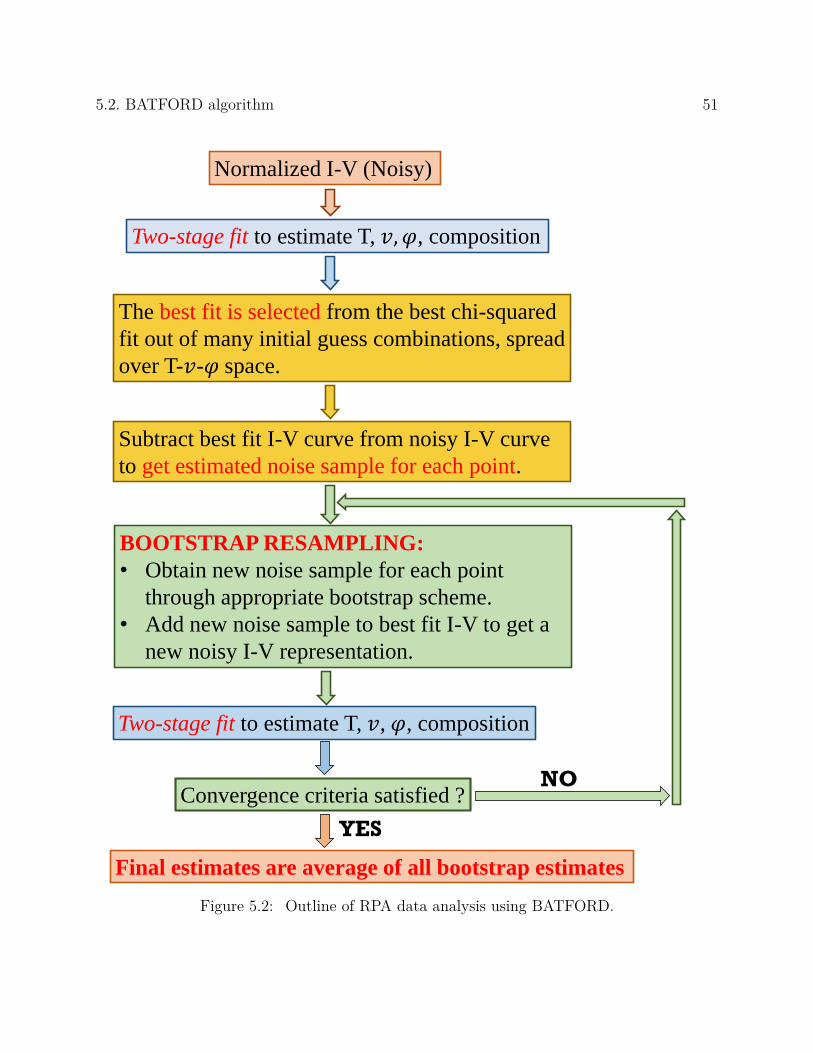
5.2. BATFORD algorithm 51
Normalized I-V (Noisy)
Two-stage fit to estimate T, 𝑣, 𝜑, composition
The best fit is selected from the best chi-squared
fit out of many initial guess combinations, spread
over T-𝑣-𝜑 space.
Subtract best fit I-V curve from noisy I-V curve
to get estimated noise sample for each point.
BOOTSTRAP RESAMPLING:
• Obtain new noise sample for each point
through appropriate bootstrap scheme.
• Add new noise sample to best fit I-V to get a
new noisy I-V representation.
Two-stage fit to estimate T, 𝑣, 𝜑, composition
Convergence criteria satisfied ?NO
Final estimates are average of all bootstrap estimates
YES
Figure 5.2: Outline of RPA data analysis using BATFORD.
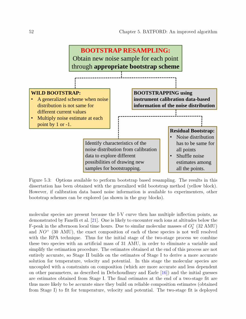
52 Chapter 5. BATFORD: An improved algorithm
BOOTSTRAP RESAMPLING:
Obtain new noise sample for each point
through appropriate bootstrap scheme
WILD BOOTSTRAP:
• A generalized scheme when noise
distribution is not same for
different current values
• Multiply noise estimate at each
point by 1 or -1.
BOOTSTRAPPING using
instrument calibration data-based
information of the noise distribution
Identify characteristics of the
noise distribution from calibration
data to explore different
possibilities of drawing new
samples for bootstrapping.
Residual Bootstrap:
• Noise distribution
has to be same for
all points
• Shuffle noise
estimates among
all the points.
Figure 5.3: Options available to perform bootstrap based resampling. The results in thisdissertation has been obtained with the generalized wild bootstrap method (yellow block).However, if calibration data based noise information is available to experimenters, otherbootstrap schemes can be explored (as shown in the gray blocks).
molecular species are present because the I-V curve then has multiple inflection points, asdemonstrated by Fanelli et al. [21]. One is likely to encounter such ions at altitudes below theF-peak in the afternoon local time hours. Due to similar molecular masses of O+
2 (32 AMU)and NO+ (30 AMU), the exact composition of each of these species is not well resolvedwith the RPA technique. Thus for the initial stage of the two-stage process we combinethese two species with an artificial mass of 31 AMU, in order to eliminate a variable andsimplify the estimation procedure. The estimates obtained at the end of this process are notentirely accurate, so Stage II builds on the estimates of Stage I to derive a more accuratesolution for temperature, velocity and potential. In this stage the molecular species areuncoupled with a constraints on composition (which are more accurate and less dependenton other parameters, as described in Debchoudhury and Earle [16]) and the initial guessesare estimates obtained from Stage I. The final estimates at the end of a two-stage fit arethus more likely to be accurate since they build on reliable composition estimates (obtainedfrom Stage I) to fit for temperature, velocity and potential. The two-stage fit is deployed

5.2. BATFORD algorithm 53
for fitting each I-V curve in the BATFORD technique.
As described in Figure 5.2, the BATFORD algorithm starts out with an I-V curve that hasbeen normalized in order to exclude the linearly dependent density term from the fittingprocess. Two-stage fits are performed on the normalized I-V curve for a range of initial seedvalues for temperature, velocity and potential. The resultant fits are analyzed and the fittedparameter combination that yield the minimum chi-squared fit are selected. Throughoutthe remainder of the text, we refer to this initially fitted combination set as the ”primitive”candidate solution. These estimates define a best-fit I-V curve to the noisy input data.However, following the discussion in Section 4.4 in chapter 4, a wide range of temperature,velocity and potential estimates exist that generate I-V profiles that can lie within the noiseenvelope of this best-fit I-V. In other words, the primitive candidate solution is a functionof the noise present in the noisy profile from which we intend to estimate our parameters.The solution will thus vary with the amount and the location in the I-V profile of the noisepresent. As a simple example, noise added at the inflection point ( peak of the Maxwellianvelocity distribution ) of an I-V curve has a more significant bearing on the estimated ionvelocity than noise added to either of the plateau regions shown in Figure 4.1. The addednoise can be interpreted as simply a probabilistic output of a modeled noise distribution,and there exist equally likely samples that can be drawn from the same distribution. Thebootstrap method generates multiple samples using the error between the primitive fittedI-V (I-V obtained from the primitive solution) and the measured I-V curves, which alwaysinclude noise.
Figure 5.3 shows a number of options available through which one can obtain new samples.If precise, calibration information for the RPA instrument is available to experimentalists,then it is possible to make use of the knowledge of the noise distribution to obtain bootstrapsamples. For example, if the noise distribution estimated from the calibration data is foundto be same for all current values, then a simple residual bootstrap can be performed wherethe errors obtained at each point can simply be redistributed and added back to the primitiveI-V. In bootstrap literature, this is referred to as residual bootstrap. However, even if thenoise distributions are different for all the current measures, yet one can make use of specificcharacteristics of the estimated functional form of the distribution to generate new samplesof errors. For example, if it is found that the noise distribution is similar for current valueswithin a certain range, then one redistribute the error samples at the points where the I-Vhas measurements lying within this specific range. The idea of the bootstrap technique isto generate new samples from the errors that have the same probability as the values theyare generated from. In our study, from the calibration-based noise model elaborated insection 2.3 in chapter 2, it is seen that a different standard deviation and hence a Gaussiandistribution with different parameters is associated with each point of the I-V curve, since thenoise added is a function of the current value. Thus we choose the wild bootstrap method asthe appropriate bootstrap technique [42] to resample the noise files. It generates new samplesby multiplying the measured noise estimate for every retarding voltage sample randomly by±1, as summarized in the yellow block of Figure 5.3. This is a widely generalized bootstrap

54 Chapter 5. BATFORD: An improved algorithm
technique that only assumes a symmetric noise distribution for every current measurementalong a sweep and does not require specific knowledge about the distribution. Thus thistechnique can also be used for analyzing data from an RPA whose noise distribution iscompletely unknown. Since any sample drawn from a symmetric distribution has an equalprobability of occurrence as its negative counterpart, all bootstrap samples represent equallylikely choices from the same unknown noise distribution. An improved bootstrap resamplingscheme can be used if some details of the statistics of the noise distribution (e.g., fromcalibration data) are available to the experimenter.
The bootstrap noise samples are drawn and added back to the primitive fitted I-V, and theresulting noisy I-Vs are valid representations of the measured noisy I-V curve that are equallylikely to have been encountered at the same instant. These equally likely noisy I-Vs aretreated with the two-stage analysis method. The averages of the parameter values estimatedat the end of the bootstrap iterations are used as the final estimates of the parameters.Analysis of a single I-V curve can yield a parameter combination for which the sum of thesquare errors is minimized, but the combination is far from the actual solution. Thus theaverage of the estimates from all the bootstrap generated noisy I-V representations helpsto remove the bias associated with a particular sample of noisy I-V curve. In this way theBATFORD algorithm addresses the issues mentioned in chapter 4.
5.2.1 BATFORD convergence criterion
The convergence criterion is used to determine when to stop taking samples and choose a finalset of parameters. Ideally this is done autonomously, so that human bias is not introduced.Simulations show that while the evolution of the average of the estimates at the end of eachbootstrap loop varies from case to case, the trend saturates after a certain stage. Davidson[14] shows that errors due to the RPA grid geometry alone cannot be resolved definitively tobetter than 21 K for temperature, and 35 m/s for velocity. These limits suggest a methodfor defining convergence to an acceptable solution:
If the velocity estimate has not changed by more than 35 m/s and the temperature estimatehas not changed by more than 21 K, then it is appropriate to stop the analysis and declarethe average of the individual bootstrap estimates up to this point as final estimates.
We use this approach to check for convergence, starting after 150 iterations. After 150bootstraps, the average estimates obtained 50 iterations prior to this stage are considered.If the two criteria mentioned above are not satisfied, 50 more bootstrap iterations are runand rechecked against the convergence criteria. A maximum of 500 bootstrap iterationsare allowed. If convergence is not attained within 500 iterations for analysis of a particularI-V, a flag is set to indicate that the results in this case should be used with caution. Thespacecraft potential is not checked in the convergence criteria since the errors in potentialhave already been established to be closely tied to the errors in velocity, so that a criteriathat checks for velocity also ensures a reasonable potential convergence. Thus in summary,
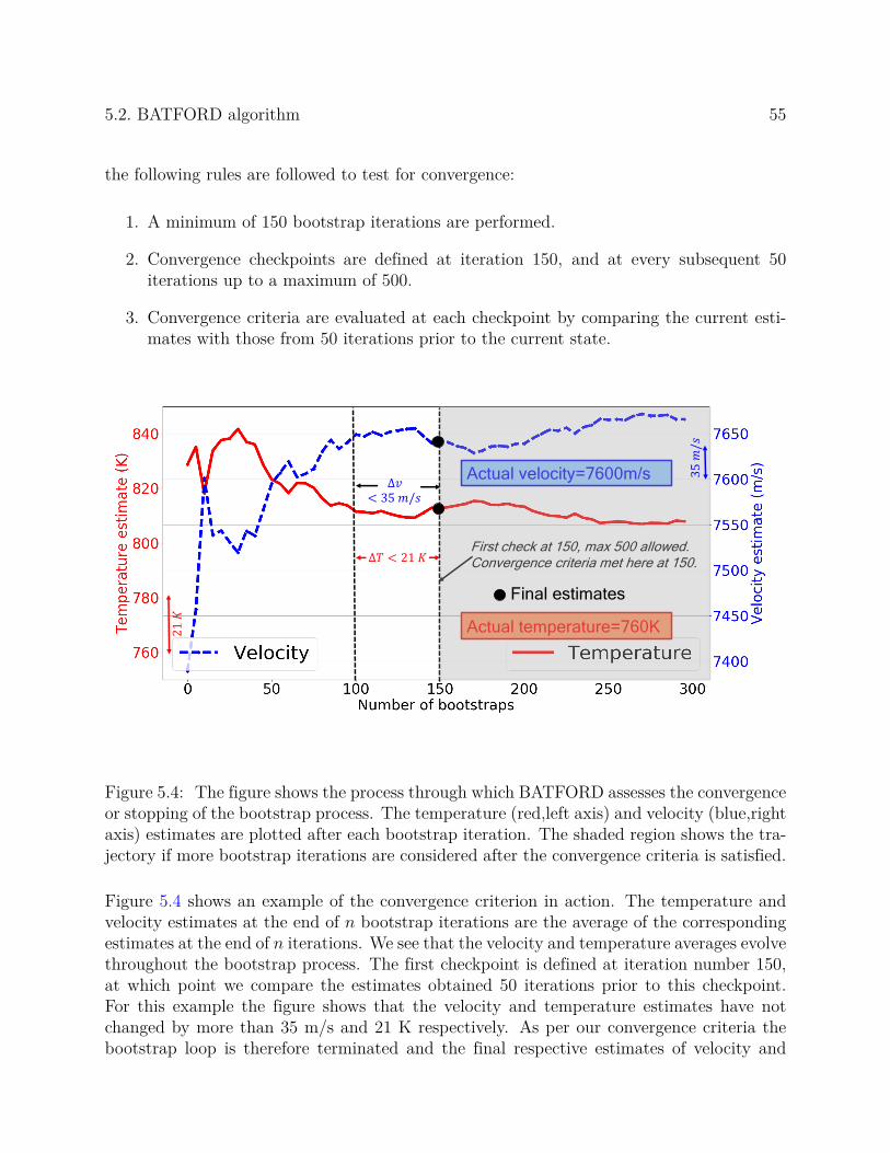
5.2. BATFORD algorithm 55
the following rules are followed to test for convergence:
1. A minimum of 150 bootstrap iterations are performed.
2. Convergence checkpoints are defined at iteration 150, and at every subsequent 50iterations up to a maximum of 500.
3. Convergence criteria are evaluated at each checkpoint by comparing the current esti-mates with those from 50 iterations prior to the current state.
Actual temperature=760K
Actual velocity=7600m/s
First check at 150, max 500 allowed.Convergence criteria met here at 150.∆𝑇 < 21 𝐾
∆𝑣< 35 𝑚/𝑠
Final estimates
21𝐾
35𝑚/𝑠
Figure 5.4: The figure shows the process through which BATFORD assesses the convergenceor stopping of the bootstrap process. The temperature (red,left axis) and velocity (blue,rightaxis) estimates are plotted after each bootstrap iteration. The shaded region shows the tra-jectory if more bootstrap iterations are considered after the convergence criteria is satisfied.
Figure 5.4 shows an example of the convergence criterion in action. The temperature andvelocity estimates at the end of n bootstrap iterations are the average of the correspondingestimates at the end of n iterations. We see that the velocity and temperature averages evolvethroughout the bootstrap process. The first checkpoint is defined at iteration number 150,at which point we compare the estimates obtained 50 iterations prior to this checkpoint.For this example the figure shows that the velocity and temperature estimates have notchanged by more than 35 m/s and 21 K respectively. As per our convergence criteria thebootstrap loop is therefore terminated and the final respective estimates of velocity and

56 Chapter 5. BATFORD: An improved algorithm
temperature are 7646 m/s and 808 K. These are indicated by black dots in the figure. Sincethis is an example from our simulation dataset and we know the actual parameter values, it isinteresting to see that the evolution of bootstraps initially decreases the errors and guides thefinal estimate closer to the true solutions. However after ∼ 100 iterations the estimates ceaseto converge toward the true solutions, which is indicative of the level of ambiguity createdby the noise. For the sake of completeness, we also plot the trajectory up to the maximumof 500 iterations, and we notice that evolution of the BATFORD estimates tends to saturate(again, within the engineering limits defined) after an initial period of high fluctuations.Statistically this signifies that a considerable number of reliable parameter combinations aregeophysically compliant, and it indicates the uncertainty created by a number of equallyrepresentative noisy scenarios. Although the figure shows only one example, it serves toillustrate the difficulties associated with statistical inferences in the presence of noise. Weshall return to the detailed discussion of the convergence criterion in section 7.2.

Chapter 6
Comparative studies of the newalgorithm
6.1 A generalized dataset
In order to test the effectiveness of BATFORD, a new generalized dataset is developed. Weneed a new dataset particularly because chapter 4 showed that the error in the estimates isheavily dependent on the manner in which noise is added to the I-V curve. Two noise samplesdrawn from the same distribution can affect the I-V curve in widely different ways, leadingto estimates that are far from each other in the whole parameter space. Thus a new datasetfor our simulation study should incorporate multiple noisy I-V curves corresponding to thesame noise-free ideal I-V. The dataset that was previously simulated in Chapter 3 (based onexpected I-Vs from a realistic orbit) encompassed numerous parameter combinations. If weallow a significant number of noisy I-V representations for ideal I-Vs from one entire orbit,the computational time for the study is greatly increased. Thus we limit the scope of thenew dataset to representative I-Vs simulated from the expected values of temperature anddensities outlined in section 3.6. The range of parameters presented in Figure 3.14 encom-pass active and quiet conditions in solstice and equinox, and also factor in the local timedependence. Using this information we choose, for the new dataset, 100 parameter combi-nations that include randomized permutations of physically reasonable parameter values inorder to carry out a comprehensive study of the RPA curve-fitting algorithm.
The ion temperatures are drawn either from a normal distribution with mean value of 800K and a standard deviation of 65 K that represent quiescent cases, or from another normaldistribution representing an active case, with mean and standard deviation of 1200 K and 40K respectively. The two distributions are chosen with a 95% preference for temperatures be-ing drawn from the quiescent temperature distribution. The histogram for the temperaturesinducted into the new dataset are shown in Figure 6.1.
For a fixed RPA geometry the ambient ion densities dictate the SNRs encountered; weintentionally focus on low-density cases for the new dataset. The idea is to test cases whereSNRs are low so that errors are inherently high, as discussed in 3.3. Thus ion densities aredrawn from a log-normal distribution in base 10, with mean 4.8 and standard deviation 0.5,resulting in densities from ∼ 103 - ∼ 106 cm−3. Figure 6.2 shows the distribution of the100 densities on a logarithmic independent axis. For a normal probability density function
57
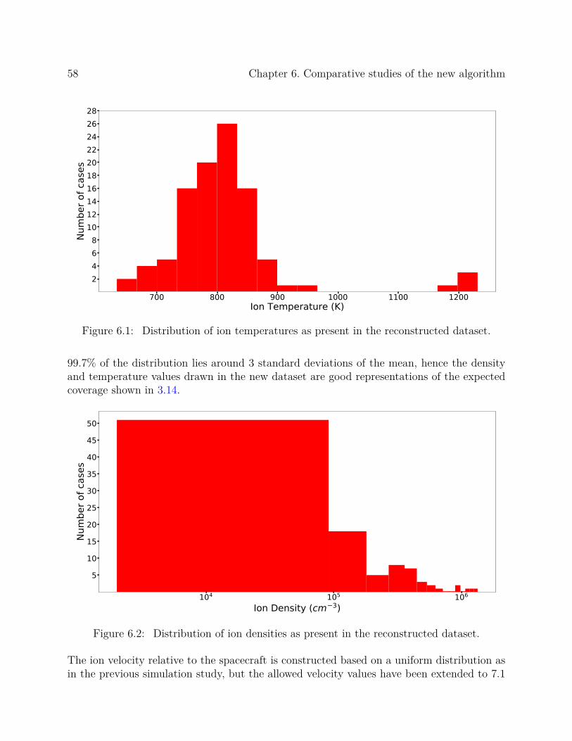
58 Chapter 6. Comparative studies of the new algorithm
700 800 900 1000 1100 1200Ion Temperature (K)
2468
10121416182022242628
Num
ber o
f cas
es
Figure 6.1: Distribution of ion temperatures as present in the reconstructed dataset.
99.7% of the distribution lies around 3 standard deviations of the mean, hence the densityand temperature values drawn in the new dataset are good representations of the expectedcoverage shown in 3.14.
104 105 106
Ion Density (cm 3)
5
10
15
20
25
30
35
40
45
50
Num
ber o
f cas
es
Figure 6.2: Distribution of ion densities as present in the reconstructed dataset.
The ion velocity relative to the spacecraft is constructed based on a uniform distribution asin the previous simulation study, but the allowed velocity values have been extended to 7.1
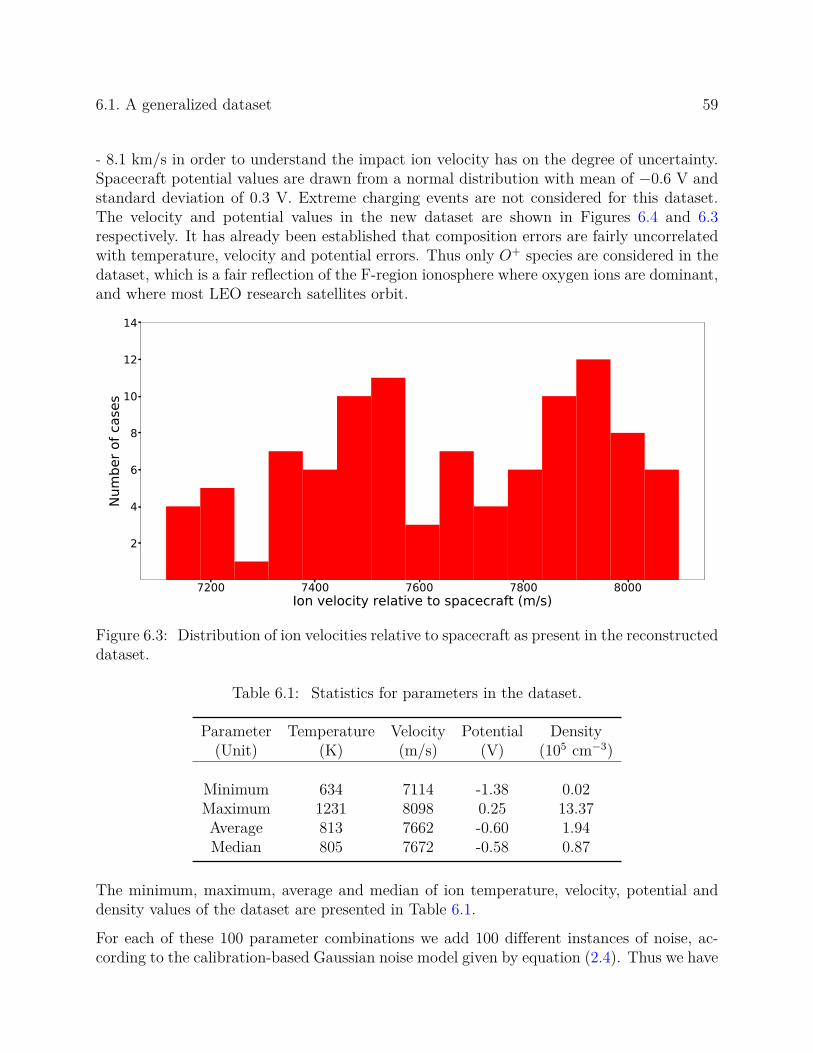
6.1. A generalized dataset 59
- 8.1 km/s in order to understand the impact ion velocity has on the degree of uncertainty.Spacecraft potential values are drawn from a normal distribution with mean of −0.6 V andstandard deviation of 0.3 V. Extreme charging events are not considered for this dataset.The velocity and potential values in the new dataset are shown in Figures 6.4 and 6.3respectively. It has already been established that composition errors are fairly uncorrelatedwith temperature, velocity and potential errors. Thus only O+ species are considered in thedataset, which is a fair reflection of the F-region ionosphere where oxygen ions are dominant,and where most LEO research satellites orbit.
7200 7400 7600 7800 8000Ion velocity relative to spacecraft (m/s)
2
4
6
8
10
12
14
Num
ber o
f cas
es
Figure 6.3: Distribution of ion velocities relative to spacecraft as present in the reconstructeddataset.
Table 6.1: Statistics for parameters in the dataset.
Parameter Temperature Velocity Potential Density(Unit) (K) (m/s) (V) (105 cm−3)
Minimum 634 7114 -1.38 0.02Maximum 1231 8098 0.25 13.37Average 813 7662 -0.60 1.94Median 805 7672 -0.58 0.87
The minimum, maximum, average and median of ion temperature, velocity, potential anddensity values of the dataset are presented in Table 6.1.
For each of these 100 parameter combinations we add 100 different instances of noise, ac-cording to the calibration-based Gaussian noise model given by equation (2.4). Thus we have

60 Chapter 6. Comparative studies of the new algorithm
1.4 1.2 1.0 0.8 0.6 0.4 0.2 0.0 0.2Spacecraft Potential (V)
2
4
6
8
10
12
14
16
Num
ber o
f cas
es
Figure 6.4: Distribution of spacecraft potentials as present in the reconstructed dataset.
a total of 10000 instances in the dataset, all of which correspond to a system temperature of25◦C. The noise-floor is set to 100 pA for all these cases. When analyzing these sets of noisyI-V curves, measurements below the noise-floor are ignored because measurements cannot betrusted when the noise level dominates the signal level. This approach is commonly used byexperimenters working with real spaceflight data. We intentionally select 100 noise cases foreach parameter combination, so that any interpreted result for an I-V curve is statisticallysignificant. Analyzing multiple representative noisy I-V curves is essential to drawing anydefinitive conclusion about the effectiveness of the applied algorithm.
6.2 Results from the simulated dataset
To test the performance of BATFORD, we run the algorithm on the simulated datasetdescribed in section 6.1, and we obtain errors for each of the estimated parameters. Inorder to understand how BATFORD compares to a standard curve fitting algorithm, weapply a simple traditional Levenberg Marquardt routine to the same dataset. For the sakeof fair comparison, both methods are seeded with the same set of initial guesses for all theinferred parameters: ion temperature, ram velocity and spacecraft potential. The traditionalalgorithm has feasibility bounds that are same as BATFORD [46]. In other words, bothalgorithms are applied to find solutions in the same geophysically reasonable parameterspace.
The fitted parameters for both the traditional algorithm and BATFORD are recorded and
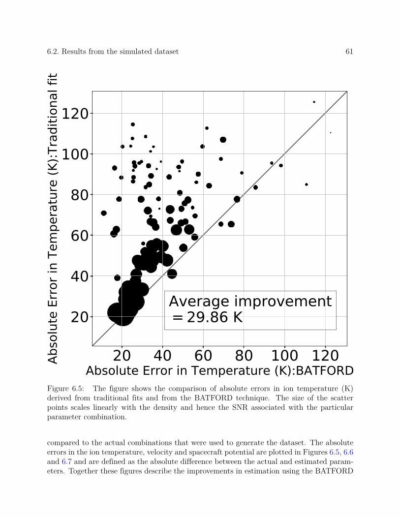
6.2. Results from the simulated dataset 61
20 40 60 80 100 120Absolute Error in Temperature (K):BATFORD
20
40
60
80
100
120
Abso
lute
Erro
r in
Tem
pera
ture
(K):T
radi
tiona
l fit
Average improvement= 29.86 K
Figure 6.5: The figure shows the comparison of absolute errors in ion temperature (K)derived from traditional fits and from the BATFORD technique. The size of the scatterpoints scales linearly with the density and hence the SNR associated with the particularparameter combination.
compared to the actual combinations that were used to generate the dataset. The absoluteerrors in the ion temperature, velocity and spacecraft potential are plotted in Figures 6.5, 6.6and 6.7 and are defined as the absolute difference between the actual and estimated param-eters. Together these figures describe the improvements in estimation using the BATFORD
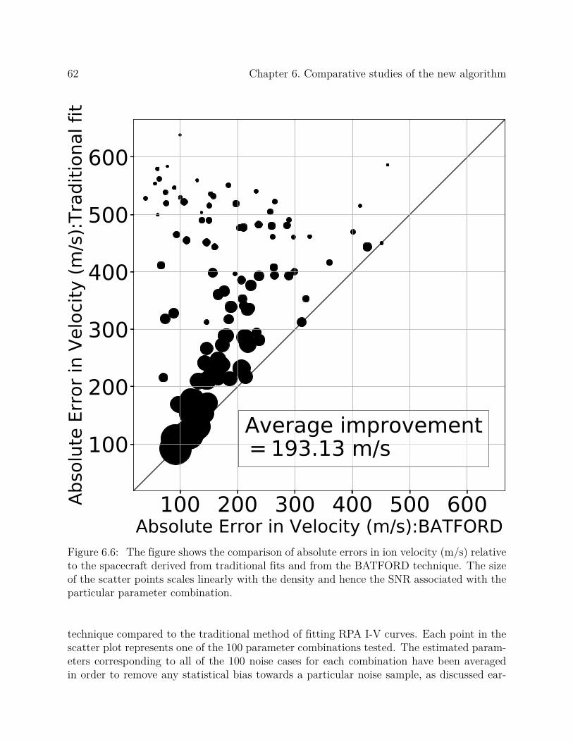
62 Chapter 6. Comparative studies of the new algorithm
100 200 300 400 500 600Absolute Error in Velocity (m/s):BATFORD
100
200
300
400
500
600
Abso
lute
Erro
r in
Velo
city
(m/s
):Tra
ditio
nal f
it
Average improvement= 193.13 m/s
Figure 6.6: The figure shows the comparison of absolute errors in ion velocity (m/s) relativeto the spacecraft derived from traditional fits and from the BATFORD technique. The sizeof the scatter points scales linearly with the density and hence the SNR associated with theparticular parameter combination.
technique compared to the traditional method of fitting RPA I-V curves. Each point in thescatter plot represents one of the 100 parameter combinations tested. The estimated param-eters corresponding to all of the 100 noise cases for each combination have been averagedin order to remove any statistical bias towards a particular noise sample, as discussed ear-

6.2. Results from the simulated dataset 63
0.1 0.2 0.3 0.4 0.5 0.6 0.7 0.8Absolute Error in Potential (V):BATFORD
0.1
0.2
0.3
0.4
0.5
0.6
0.7
0.8
Abso
lute
Erro
r in
Pote
ntia
l (V)
:Tra
ditio
nal f
it
Average improvement= 0.25 V
Figure 6.7: The figure shows the comparison of absolute errors in spacecraft potential (V)derived from traditional fits and from the BATFORD technique. The size of the scatterpoints scales linearly with the density and hence the SNR associated with the particularparameter combination.
lier. The largest scatter points correspond to I-V cases where the ion density is the highest,which correlates with the largest collected currents, and therefore the highest signal-to-noiseratios (SNR). The diagonal solid black line denotes the locus of points where the errors forBATFORD and for the traditional approach are equal. The domain to the left and aboveof this line (y > x) is where the errors in estimation by BATFORD are smaller than those

64 Chapter 6. Comparative studies of the new algorithm
20 40 60 80 100Standard deviation in Temperature (K):BATFORD
20
40
60
80
100
Stan
dard
dev
iatio
n in
Tem
pera
ture
(K):T
radi
tiona
l fit
Average improvement= 18.46 K
Figure 6.8: The standard deviations in temperature errors obtained by BATFORD plottedagainst those obtained by a traditional fit.
from the traditional fit. Similarly the points in the region to the lower right region denotescases where the BATFORD approach is less accurate than the traditional method.
The results show that the BATFORD method significantly outperforms the traditionalmethod by producing a larger number of more accurate estimates of temperature, veloc-ity and potential. In some instances the ion temperature errors are larger as estimated by
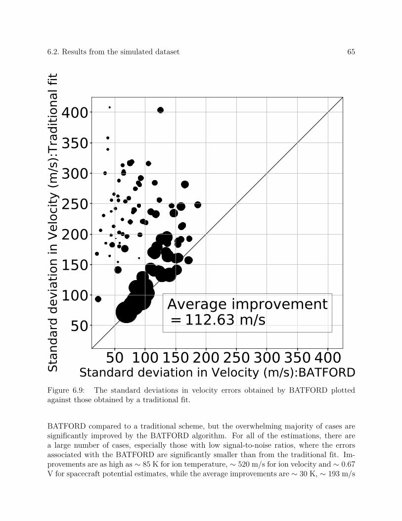
6.2. Results from the simulated dataset 65
50 100 150 200 250 300 350 400Standard deviation in Velocity (m/s):BATFORD
50
100
150
200
250
300
350
400
Stan
dard
dev
iatio
n in
Vel
ocity
(m/s
):Tra
ditio
nal f
it
Average improvement= 112.63 m/s
Figure 6.9: The standard deviations in velocity errors obtained by BATFORD plottedagainst those obtained by a traditional fit.
BATFORD compared to a traditional scheme, but the overwhelming majority of cases aresignificantly improved by the BATFORD algorithm. For all of the estimations, there area large number of cases, especially those with low signal-to-noise ratios, where the errorsassociated with the BATFORD are significantly smaller than from the traditional fit. Im-provements are as high as ∼ 85 K for ion temperature, ∼ 520 m/s for ion velocity and ∼ 0.67V for spacecraft potential estimates, while the average improvements are ∼ 30 K, ∼ 193 m/s

66 Chapter 6. Comparative studies of the new algorithm
0.1 0.2 0.3 0.4 0.5Standard deviation in Potential (V):BATFORD
0.1
0.2
0.3
0.4
0.5
Stan
dard
dev
iatio
n in
Pot
entia
l (V)
:Tra
ditio
nal f
it
Average improvement= 0.14 V
Figure 6.10: The standard deviations in spacecraft potential errors obtained by BATFORDplotted against those obtained by a traditional fit.
and ∼ 0.25 V. The trend for the spacecraft potential is similar to the velocity errors, asexpected from the analytical interdependence of the two parameters.
In Figures 6.8, 6.9 and 6.10 we show respectively the standard deviations in the average errorsin temperature, velocity and potential. These standard deviation measurements correspondto the error bars which where were not shown in the prior figures for the sake of clarity.
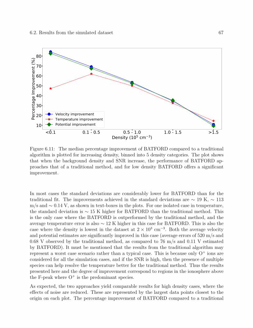
6.2. Results from the simulated dataset 67
<0.1 0.1 - 0.5 0.5 - 1.0 1.0 - 1.5 >1.5Density (105 cm 3)
10
20
30
40
50
60
70
80
Perc
enta
ge Im
prov
emen
t (%
)
Velocity improvementTemperature improvementPotential improvement
Figure 6.11: The median percentage improvement of BATFORD compared to a traditionalalgorithm is plotted for increasing density, binned into 5 density categories. The plot showsthat when the background density and SNR increase, the performance of BATFORD ap-proaches that of a traditional method, and for low density BATFORD offers a significantimprovement.
In most cases the standard deviations are considerably lower for BATFORD than for thetraditional fit. The improvements achieved in the standard deviations are ∼ 19 K, ∼ 113m/s and ∼ 0.14 V, as shown in text-boxes in the plots. For one isolated case in temperature,the standard deviation is ∼ 15 K higher for BATFORD than the traditional method. Thisis the only case where the BATFORD is outperformed by the traditional method, and theaverage temperature error is also ∼ 12 K higher in this case for BATFORD. This is also thecase where the density is lowest in the dataset at 2 × 103 cm−3. Both the average velocityand potential estimates are significantly improved in this case (average errors of 520 m/s and0.68 V observed by the traditional method, as compared to 76 m/s and 0.11 V estimatedby BATFORD). It must be mentioned that the results from the traditional algorithm mayrepresent a worst case scenario rather than a typical case. This is because only O+ ions areconsidered for all the simulation cases, and if the SNR is high, then the presence of multiplespecies can help resolve the temperature better for the traditional method. Thus the resultspresented here and the degree of improvement correspond to regions in the ionosphere abovethe F-peak where O+ is the predominant species.
As expected, the two approaches yield comparable results for high density cases, where theeffects of noise are reduced. These are represented by the largest data points closest to theorigin on each plot. The percentage improvement of BATFORD compared to a traditional
68 Chapter 6. Comparative studies of the new algorithm
technique is shown in Figure 6.11. The densities present in the dataset are binned into 5categories and the median percentage improvement recorded by BATFORD compared tothe traditional method in each category is shown for temperature, velocity and spacecraftpotential estimates. The figure shows that for high density, high SNR instances (ion densitylarger than 1.5 × 105 cm−3), the median improvement margin decreases to around 10% forvelocity and potential and around 20% for temperature. For low SNR (low density casesless than 104 cm−3) BATFORD outperforms a traditional algorithm by a margin of ∼ 85%for velocity and potential estimation, and around 50% for temperature. In one of the lowerdensity cases (less than 104 cm−3) , BATFORD is seen to record a higher temperature errorthan the traditional method. It is because of this particular case that the temperatureestimate improvement profile is not decreasing with SNR as is the case with the velocity andpotential estimates. The similar nature of the degree of improvement in the potential andvelocity estimates further establishes the linear correlation in the estimates for these twoparameters. For analyzing a single I-V curve, BATFORD produces more estimates whichindividually portray this linear dependency in errors and hence this is also mirrored in theaverage of these individual estimates which we declare as the final estimates.

Chapter 7
Analysis and Discussion
7.1 Summary of findings
Analyzing data from orbiting RPAs in the presence of noise is a significant challenge, andone that deserves closer investigation. An RPA design by itself produces uncertainties owingto the non-uniform potential distribution across the grid surfaces, resulting in alterations tothe incoming ion distribution [8, 9]. Deviations from an idealized Maxwellian distributioncoupled with inherent electronic noise further compound the curve-fitting problem. The I-Vequation that results from assuming a Maxwellian distribution at orbital velocities is heav-ily dependent on the interplay between ion velocity, temperature and spacecraft potential.Depending on the noise level, one can expect significant errors in these parameters whenanalyzing an I-V curve. As discussed in chapter 4, if a noisy I-V curve is analyzed to infera velocity-potential pair, then there exist many such pairs that also lie within the noiseenvelope of the best-fit I-V. By analytically approximating the relationship between thesevelocity-potential pairs we find that depending on the initial condition and the noise added,the inferred velocity or potential can cover a wide range of values. In other words, manycandidate solutions will lead to I-V curves that lie within the noise envelope. The challenge isto autonomously infer the most likely solution from among these equally plausible solutions,thereby avoiding biases that could be introduced by subjective human constraints.
The accuracy of estimates is a function of both the overall noise level and the particularway noise is distributed along the I-V profile. For an assumed overall noise distribution,we can draw two noise samples which lead to widely different solutions, even for the sameinitial seeds. This imparts a lack of confidence in the estimates obtained from a single runof the I-V analysis algorithm because the noisy I-V input is just one single representationamong equally valid possibilities. In statistics a general solution is to perform resamplingto generate estimates that are unbiased towards a particular sample. Our improved generalalgorithm (BATFORD) makes use of a resampling technique called wild bootstrap to obtainfurther representations of a noisy I-V curve, all of which are guaranteed to be equally likely.Analyses of all these representations for a wide range of initial guesses eliminates the biastowards a particular solution.
In order to generate a dataset of simulated noisy I-Vs to test our algorithm, we developeda real instrument calibration-based noise model in Section 2. The noise model is seen tofollow a Gaussian distribution that is dependent on the current measurement, and this is
69
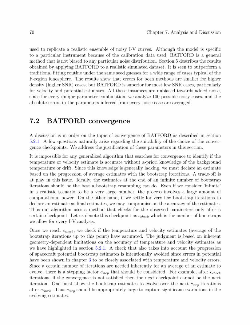
70 Chapter 7. Analysis and Discussion
used to replicate a realistic ensemble of noisy I-V curves. Although the model is specificto a particular instrument because of the calibration data used, BATFORD is a generalmethod that is not biased to any particular noise distribution. Section 5 describes the resultsobtained by applying BATFORD to a realistic simulated dataset. It is seen to outperform atraditional fitting routine under the same seed guesses for a wide range of cases typical of theF-region ionosphere. The results show that errors for both methods are smaller for higherdensity (higher SNR) cases, but BATFORD is superior for most low SNR cases, particularlyfor velocity and potential estimates. All these instances are unbiased towards added noise,since for every unique parameter combination, we analyze 100 possible noisy cases, and theabsolute errors in the parameters inferred from every noise case are averaged.
7.2 BATFORD convergence
A discussion is in order on the topic of convergence of BATFORD as described in section5.2.1. A few questions naturally arise regarding the suitability of the choice of the conver-gence checkpoints. We address the justification of these parameters in this section.
It is impossible for any generalized algorithm that searches for convergence to identify if thetemperature or velocity estimate is accurate without a-priori knowledge of the backgroundtemperature or drift. Since this knowledge is generally lacking, we must declare an estimatebased on the progression of average estimates with the bootstrap iterations. A trade-off isat play in this issue. Ideally, the estimates at the end of an infinite number of bootstrapiterations should be the best a bootstrap resampling can do. Even if we consider ’infinite’in a realistic scenario to be a very large number, the process involves a large amount ofcomputational power. On the other hand, if we settle for very few bootstrap iterations todeclare an estimate as final estimates, we may compromise on the accuracy of the estimates.Thus our algorithm uses a method that checks for the observed parameters only after acertain checkpoint. Let us denote this checkpoint as ccheck which is the number of bootstrapswe allow for every I-V analysis.
Once we reach ccheck, we check if the temperature and velocity estimates (average of thebootstrap iterations up to this point) have saturated. The judgment is based on inherentgeometry-dependent limitations on the accuracy of temperature and velocity estimates aswe have highlighted in section 5.2.1. A check that also takes into account the progressionof spacecraft potential bootstrap estimates is intentionally avoided since errors in potentialhave been shown in chapter 3 to be closely associated with temperature and velocity errors.Since a certain number of iterations are needed inherently for an average of an estimate toevolve, there is a stepping factor cstep that should be considered. For example, after ccheckiterations, if the convergence is not satisfied then the next checkpoint cannot be the nextiteration. One must allow the bootstrap estimates to evolve over the next cstep iterationsafter ccheck. Thus cstep should be appropriately large to capture significance variations in theevolving estimates.
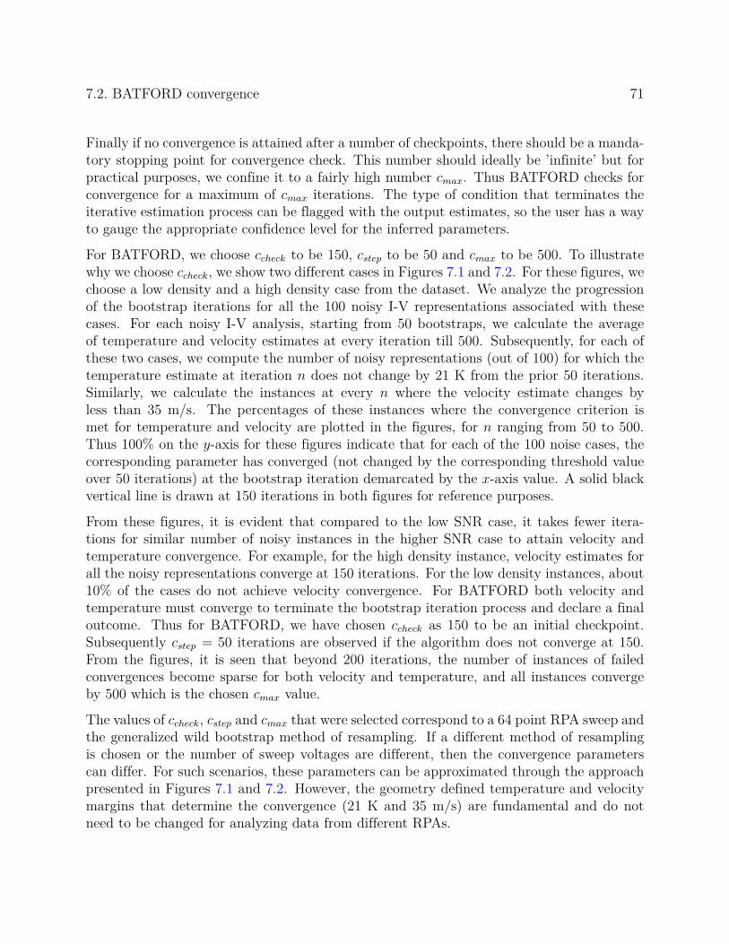
7.2. BATFORD convergence 71
Finally if no convergence is attained after a number of checkpoints, there should be a manda-tory stopping point for convergence check. This number should ideally be ’infinite’ but forpractical purposes, we confine it to a fairly high number cmax. Thus BATFORD checks forconvergence for a maximum of cmax iterations. The type of condition that terminates theiterative estimation process can be flagged with the output estimates, so the user has a wayto gauge the appropriate confidence level for the inferred parameters.
For BATFORD, we choose ccheck to be 150, cstep to be 50 and cmax to be 500. To illustratewhy we choose ccheck, we show two different cases in Figures 7.1 and 7.2. For these figures, wechoose a low density and a high density case from the dataset. We analyze the progressionof the bootstrap iterations for all the 100 noisy I-V representations associated with thesecases. For each noisy I-V analysis, starting from 50 bootstraps, we calculate the averageof temperature and velocity estimates at every iteration till 500. Subsequently, for each ofthese two cases, we compute the number of noisy representations (out of 100) for which thetemperature estimate at iteration n does not change by 21 K from the prior 50 iterations.Similarly, we calculate the instances at every n where the velocity estimate changes byless than 35 m/s. The percentages of these instances where the convergence criterion ismet for temperature and velocity are plotted in the figures, for n ranging from 50 to 500.Thus 100% on the y-axis for these figures indicate that for each of the 100 noise cases, thecorresponding parameter has converged (not changed by the corresponding threshold valueover 50 iterations) at the bootstrap iteration demarcated by the x-axis value. A solid blackvertical line is drawn at 150 iterations in both figures for reference purposes.
From these figures, it is evident that compared to the low SNR case, it takes fewer itera-tions for similar number of noisy instances in the higher SNR case to attain velocity andtemperature convergence. For example, for the high density instance, velocity estimates forall the noisy representations converge at 150 iterations. For the low density instances, about10% of the cases do not achieve velocity convergence. For BATFORD both velocity andtemperature must converge to terminate the bootstrap iteration process and declare a finaloutcome. Thus for BATFORD, we have chosen ccheck as 150 to be an initial checkpoint.Subsequently cstep = 50 iterations are observed if the algorithm does not converge at 150.From the figures, it is seen that beyond 200 iterations, the number of instances of failedconvergences become sparse for both velocity and temperature, and all instances convergeby 500 which is the chosen cmax value.
The values of ccheck, cstep and cmax that were selected correspond to a 64 point RPA sweep andthe generalized wild bootstrap method of resampling. If a different method of resamplingis chosen or the number of sweep voltages are different, then the convergence parameterscan differ. For such scenarios, these parameters can be approximated through the approachpresented in Figures 7.1 and 7.2. However, the geometry defined temperature and velocitymargins that determine the convergence (21 K and 35 m/s) are fundamental and do notneed to be changed for analyzing data from different RPAs.
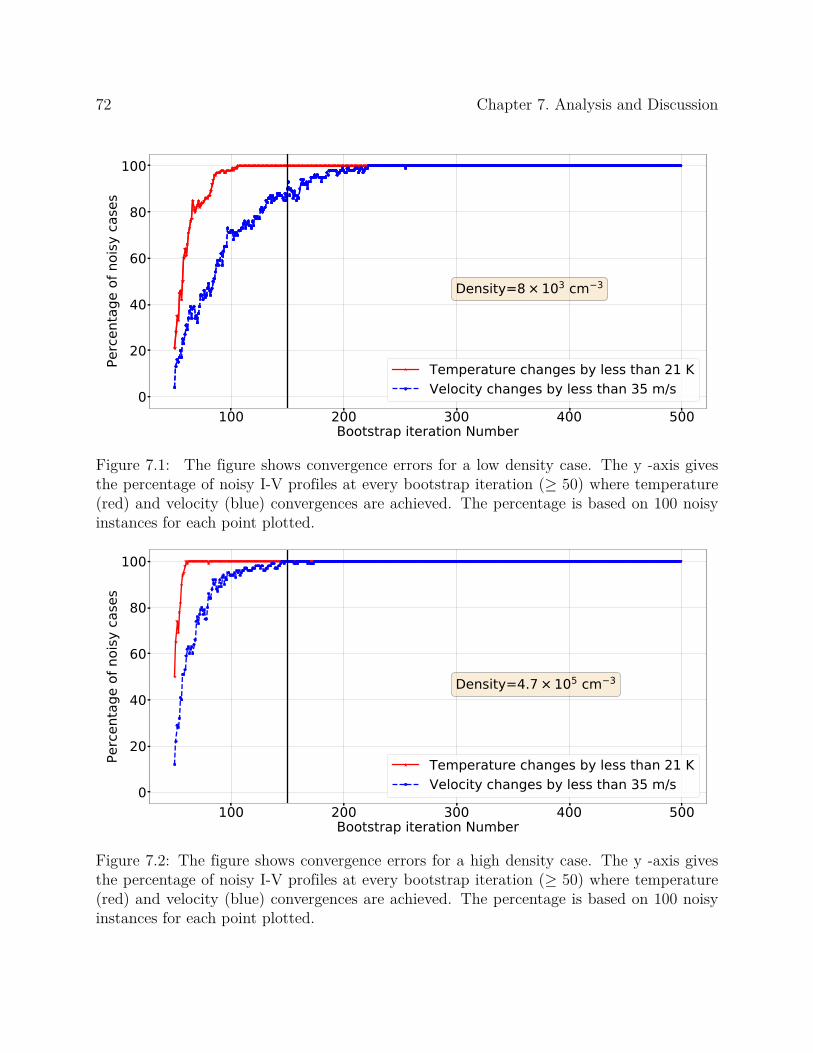
72 Chapter 7. Analysis and Discussion
100 200 300 400 500Bootstrap iteration Number
0
20
40
60
80
100
Perc
enta
ge o
f noi
sy c
ases
Density=8 × 103 cm 3
Temperature changes by less than 21 KVelocity changes by less than 35 m/s
Figure 7.1: The figure shows convergence errors for a low density case. The y -axis givesthe percentage of noisy I-V profiles at every bootstrap iteration (≥ 50) where temperature(red) and velocity (blue) convergences are achieved. The percentage is based on 100 noisyinstances for each point plotted.
100 200 300 400 500Bootstrap iteration Number
0
20
40
60
80
100
Perc
enta
ge o
f noi
sy c
ases
Density=4.7 × 105 cm 3
Temperature changes by less than 21 KVelocity changes by less than 35 m/s
Figure 7.2: The figure shows convergence errors for a high density case. The y -axis givesthe percentage of noisy I-V profiles at every bootstrap iteration (≥ 50) where temperature(red) and velocity (blue) convergences are achieved. The percentage is based on 100 noisyinstances for each point plotted.

7.3. Case study of noise effects from simulation results 73
7.3 Case study of noise effects from simulation results
In this dissertation we establish that the errors in estimation depend on how the noise isdistributed in the I-V profile. A principal reason why BATFORD provides a better estimatethan a traditional algorithm is that it leverages the idea that we can redistribute the noisethrough resampling and analyze each noisy representation separately. One would naturallybe inclined to raise the question as to what the impact of noise is for each retarding voltagevalue. We know that there is a sensitive transition region in the I-V curve that is criticallydependent on the temperature, velocity and spacecraft potential, but to properly ascertainthe relative importance of noise across this region a detailed study needs to be conducted.This is a challenging problem and one that is important to consider in designing RPAsthat can return accurate parameters from estimation. The impact of noise depends on theparameters that produce the I-V curve, so it is difficult to propose a generalized argumentwithout a rigorous study. Nevertheless, in this section we perform a primitive investigationby looking at a particular case from our simulated dataset in order to assess the relativeimpact of noise across the sensitive transition region.
We first select a case from our 100 simulated parameter combinations in the dataset presentedin section 6.1. The particular instance we present here corresponds to an ion density of 7×10³
cm−3, temperature at 692 K, with the spacecraft potential at -0.34 V and an ion velocity of7405 m/s relative to the spacecraft ram direction. For this combination, we analyze the errorsobtained in each of the 100 simulated noisy I-Vs. Figure 7.3 shows some of the highlightsof the analysis performed for this case with respect to understanding the errors observed intemperature.
Before analyzing the details of the observations made through Figure 7.3, we highlight theprocess through which the figure is obtained. Reading the right-side axis in panel A, theblack curve shows the normalized noise-free I-V curve. Next we identify the two cases outof our ensemble of 100 where the maximum and minimum temperature errors are observed.For these two noisy I-V representations we plot the signed percentage of noise with respect tothe noise-free current at each retarding voltage. The percentages are read from the left axis.The red trace shows the case corresponding to the maximum temperature error, and the bluetrace corresponds to the minimum temperature error. A positive signed percentage impliesthat a positive noise current was present at the corresponding voltage, while a negativepercentage signifies that the noise current reduced the current depicted for the noise-free I-Vcurve. The dotted horizontal line denotes the noise-free regime. As expected, the percentageof noise added increases with increasing retarding voltage due to low current values recordedas we approach the high-energy tail.
In Panel B, we show the partial derivative of the noise-free normalized current with respect totemperature. The derivative profiles are calculated numerically for a series of temperatures,with the other parameters maintained at constant values that are same as those correspond-ing to the noise-free I-V. Points P1, P2, Q1, Q2 and M are of particular significance in this

74 Chapter 7. Analysis and Discussion
P1
Q1
M
P2
Q2
A)
B)
No
ise
/Sig
na
l A
mp
litu
de
(%
)
Figure 7.3: Panel A shows the normalized noise-free current in black along the right axis foran I-V curve. The red and blue lines show the noise added to the curve for the cases that hadthe most accurate (blue) and least accurate (red) inferred temperatures. The noise addedas a percentage of the noise-free current is read from the left axis for these two cases. Thehighlighted rectangular patch shows a region important to temperature estimation where thederivatives with respect to temperature shown in panel B are also high. Important locationsare demarcated by points in Panel B while dotted vertical lines map these regions to theplot in Panel A.
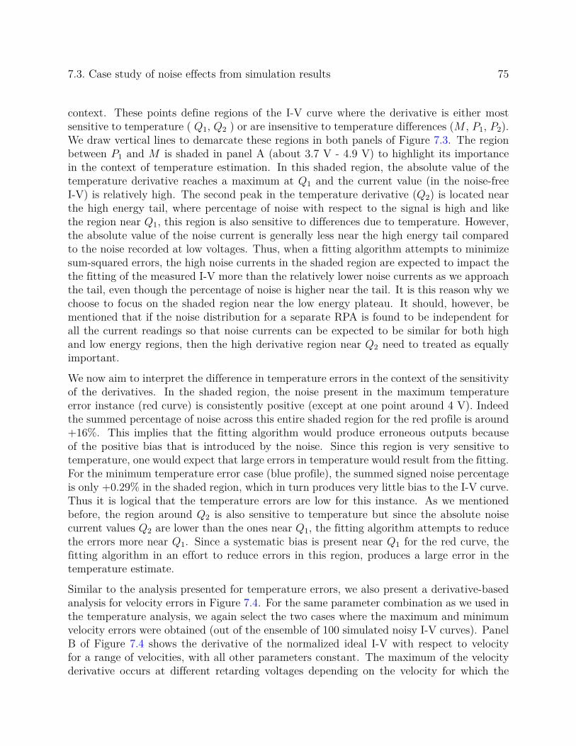
7.3. Case study of noise effects from simulation results 75
context. These points define regions of the I-V curve where the derivative is either mostsensitive to temperature ( Q1, Q2 ) or are insensitive to temperature differences (M , P1, P2).We draw vertical lines to demarcate these regions in both panels of Figure 7.3. The regionbetween P1 and M is shaded in panel A (about 3.7 V - 4.9 V) to highlight its importancein the context of temperature estimation. In this shaded region, the absolute value of thetemperature derivative reaches a maximum at Q1 and the current value (in the noise-freeI-V) is relatively high. The second peak in the temperature derivative (Q2) is located nearthe high energy tail, where percentage of noise with respect to the signal is high and likethe region near Q1, this region is also sensitive to differences due to temperature. However,the absolute value of the noise current is generally less near the high energy tail comparedto the noise recorded at low voltages. Thus, when a fitting algorithm attempts to minimizesum-squared errors, the high noise currents in the shaded region are expected to impact thethe fitting of the measured I-V more than the relatively lower noise currents as we approachthe tail, even though the percentage of noise is higher near the tail. It is this reason why wechoose to focus on the shaded region near the low energy plateau. It should, however, bementioned that if the noise distribution for a separate RPA is found to be independent forall the current readings so that noise currents can be expected to be similar for both highand low energy regions, then the high derivative region near Q2 need to treated as equallyimportant.
We now aim to interpret the difference in temperature errors in the context of the sensitivityof the derivatives. In the shaded region, the noise present in the maximum temperatureerror instance (red curve) is consistently positive (except at one point around 4 V). Indeedthe summed percentage of noise across this entire shaded region for the red profile is around+16%. This implies that the fitting algorithm would produce erroneous outputs becauseof the positive bias that is introduced by the noise. Since this region is very sensitive totemperature, one would expect that large errors in temperature would result from the fitting.For the minimum temperature error case (blue profile), the summed signed noise percentageis only +0.29% in the shaded region, which in turn produces very little bias to the I-V curve.Thus it is logical that the temperature errors are low for this instance. As we mentionedbefore, the region around Q2 is also sensitive to temperature but since the absolute noisecurrent values Q2 are lower than the ones near Q1, the fitting algorithm attempts to reducethe errors more near Q1. Since a systematic bias is present near Q1 for the red curve, thefitting algorithm in an effort to reduce errors in this region, produces a large error in thetemperature estimate.
Similar to the analysis presented for temperature errors, we also present a derivative-basedanalysis for velocity errors in Figure 7.4. For the same parameter combination as we used inthe temperature analysis, we again select the two cases where the maximum and minimumvelocity errors were obtained (out of the ensemble of 100 simulated noisy I-V curves). PanelB of Figure 7.4 shows the derivative of the normalized ideal I-V with respect to velocityfor a range of velocities, with all other parameters constant. The maximum of the velocityderivative occurs at different retarding voltages depending on the velocity for which the
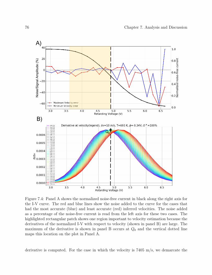
76 Chapter 7. Analysis and Discussion
B)
A)
Q0
No
ise
/Sig
na
l A
mp
litu
de
(%
)
Figure 7.4: Panel A shows the normalized noise-free current in black along the right axis forthe I-V curve. The red and blue lines show the noise added to the curve for the cases thathad the most accurate (blue) and least accurate (red) inferred velocities. The noise addedas a percentage of the noise-free current is read from the left axis for these two cases. Thehighlighted rectangular patch shows one region important to velocity estimation because thederivatives of the normalized I-V with respect to velocity (shown in panel B) are large. Themaximum of the derivative is shown in panel B occurs at Q0 and the vertical dotted linemaps this location on the plot in Panel A.
derivative is computed. For the case in which the velocity is 7405 m/s, we demarcate the
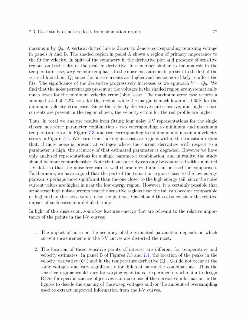
7.3. Case study of noise effects from simulation results 77
maximum by Q0. A vertical dotted line is drawn to denote corresponding retarding voltagein panels A and B. The shaded region in panel A shows a region of primary importance tothe fit for velocity. In spite of the symmetry in the derivative plot and presence of sensitiveregions on both sides of the peak in derivative, in a manner similar to the analysis in thetemperature case, we give more emphasis to the noise measurements present to the left of thevertical line about Q0 since the noise currents are higher and hence more likely to affect thefits. The significance of the derivative progressively increases as we approach V = Q0. Wefind that the noise percentages present at the voltages in the shaded region are systematicallymuch lower for the minimum velocity error (blue) case. The maximum error case records asummed total of -22% noise for this region, while the margin is much lower at -1.05% for theminimum velocity error case. Since the velocity derivatives are sensitive, and higher noisecurrents are present in the region shown, the velocity errors for the red profile are higher.
Thus, in total we analyze results from fitting four noisy I-V representations for the singlechosen noise-free parameter combination - two corresponding to minimum and maximumtemperature errors in Figure 7.3, and two corresponding to minimum and maximum velocityerrors in Figure 7.4. We learn from looking at sensitive regions within the transition regionthat, if more noise is present at voltages where the current derivative with respect to aparameter is high, the accuracy of that estimated parameter is degraded. However we haveonly analyzed representations for a single parameter combination, and in reality, the studyshould be more comprehensive. Note that such a study can only be conducted with simulatedI-V data so that the noise-free case is well characterized and can be used for comparison.Furthermore, we have argued that the part of the transition region closer to the low energyplateau is perhaps more significant than the one closer to the high energy tail, since the noisecurrent values are higher in near the low energy region. However, it is certainly possible thatsome stray high noise currents near the sensitive regions near the tail can become comparableor higher than the noise values near the plateau. One should thus also consider the relativeimpact of such cases in a detailed study.
In light of this discussion, some key features emerge that are relevant to the relative impor-tance of the points in the I-V curves:
1. The impact of noise on the accuracy of the estimated parameters depends on whichcurrent measurements in the I-V curves are distorted the most.
2. The location of these sensitive points of interest are different for temperature andvelocity estimates. In panel B of Figures 7.3 and 7.4, the location of the peaks in thevelocity derivative (Q0) and in the temperature derivative (Q1, Q2) do not occur at thesame voltages and vary significantly for different parameter combinations. Thus thesensitive regions would vary for varying conditions. Experimenters who aim to designRPAs for specific science objectives can make use of the derivative information in thefigures to decide the spacing of the sweep voltages and/or the amount of oversamplingused to extract improved information from the I-V curves.

78 Chapter 7. Analysis and Discussion
3. In practice, the retarding voltages are often applied through a digitally sampled D/Aconverter. Thus sensitive current samples can easily fall between successive voltagesamples. In such a case the estimation of parameters could depend on deviation incurrent due to noise at the less sensitive points. In other words, with a fixed and finitenumber of sampled points, there is no way to algorithmically minimize the impact ofnoise for all sets of parameter combinations. Increasing the number of samples in theI-V sweep reduces this problem, but does so at the expense of temporal resolution.
7.4 Application of BATFORD to Flight Data
As an additional test, we apply the BATFORD method to noisy flight data from a real RPAinstrument. The Communications/Navigation Outage Forecasting System (i.e. C/NOFS)satellite [15] was launched into a low-inclination ionospheric orbit and carried an RPA as oneof its sensors. The RPA encountered a number of instances of equatorial plasma bubbles,where the ion density drops significantly compared to the background density over spatiallengths ranging from hundreds of meters to hundreds of kilometers . Studies [30, 31, 32] havereported bubbles and plasma depletion observed by C/NOFS, and significant forays havebeen made to characterize and explain generation mechanisms for these bubbles. The densityin a deep bubble can be as low as a few hundred ions per cm3 which significantly affectsRPA measurements. In such a scenario the signal level drops sharply and the RPA recordsvery low currents. As we have discussed, in these low SNR regions the estimation processsuffers significantly. Thus there always has been a lack of confidence in parameters like iontemperature measured within plasma bubbles. The BATFORD technique can address thisissue using the resampling feature to give estimates that have a higher degree of reliability.
Figure 7.5 shows a bubble observed by C/NOFS around 1:05 UT, where the backgrounddensity at the satellite’s location drops to a low near 103 per cm3. The raw I-V curves areanalyzed using BATFORD and the traditional method, and the ion temperatures, velocitiesand densities are plotted. The scatter points are the results from fitting individual I-Vcurves, and the solid fitted lines show the profile after smoothing with a Savitzky-Golay[50]) low pass filter. The ion velocity estimates obtained from the traditional method sufferdue to the low SNR, and frequently the fitting algorithm is seen to converge to velocityestimates that are not realistic for orbital satellites. In these cases the traditional algorithmis stopped prematurely so that the final estimates are more geophysically reasonable, butcertainly cannot be trusted. Only in regions demarcated by the solid black line at the bottomof the ion velocity (second) panel does the traditional algorithm converge to values withinimposed realistic geophysical bounds. In fact, most of the C/NOFS data presented in thebubble region have been previously labeled by the experiment team with a quality flag valueof ”3”, which signifies noisy measurements where the ram velocity estimates should not betrusted.
We believe this is primarily because of the manner in which high noise affects the uncertain-

7.4. Application of BATFORD to Flight Data 79
Line denotes regions
of reasonable velocity
estimates from a
traditional RPA fit
Figure 7.5: The figure shows comparisons of results obtained in and around a low latitudeplasma bubble by applying BATFORD and a traditional fitting routine. The ion tempera-tures (top panel), ion velocities (middle panel) and ion densities (bottom panel) are shown.The blue circles denote the BATFORD estimates while the filled red stars denote thosefrom a traditional fit. The same low pass filter is applied to smooth the data for both sets ofestimates. The horizontal line at the bottom of the middle panel shows regions where the ve-locity estimates from the traditional fit cannot be trusted since the fitting algorithm tries toconverge to velocity values beyond geophysically reasonable ranges. The yellow highlightedpatch shows the deepest portions of the bubble. The estimates from the two methods differsignificantly, and the BATFORD estimates are more geophysically reasonable.
ties associated with velocity and potential estimates; a traditional autonomous fitting processcannot handle such cases intelligently. In comparison, BATFORD makes use of resamplingto produce autonomous estimates for velocity and temperature that are statistically andgeophysically reasonable. In Figure 7.5, the average difference in the estimated temperaturebetween BATFORD and the traditional method is ∼ 49 K (standard deviation of 63 K)while the mean difference in the estimated velocities is ∼ 87 m/s (standard deviation of 62m/s). Thus there are considerable differences between the estimates obtained using the twomethods.
80 Chapter 7. Analysis and Discussion
Since BATFORD is seen to be superior to the traditional method in our simulations, andsince the BATFORD estimates obtained in the bubble are physically reasonable, we concludethat BATFORD outperforms the traditional method. The density estimates do not dependon the curve-fitting process, so the estimation of the density is similar for the two approacheswith minor variations owing to the velocity dependence on the normalization factor of theI-V curves. For all the other fitted parameters the BATFORD algorithm is superior to thetraditional approach, particularly in cases with low SNR. Application of the BATFORDapproach should therefore be seriously considered for analysis of RPA data in low densityenvironments.
7.4.1 Interpretation of flight data using BATFORD
In the late phases of the C/NOFS mission it orbits in an altitude range that is not highenough to include fast H+ ions, and the the low-inclination orbit is suitable for observingequatorial plasma bubbles. The parameters inferred by the BATFORD technique in the lowSNR bubble region are seen to be significantly different from those inferred from a traditionalmethod. In fact, a large portion of the ion-velocity estimates were seen to go beyond real-istic geophysical bounds for the traditional case, while BATFORD produces geophysicallyreasonable estimates. Such cases are often treated subjectively using human interventionto constrain or change settings, but BATFORD improves the estimates objectively, withoutintervention. BATFORD has autonomous resampling capabilities that generate and analyzea number of representative I-V cases for noisy I-V curves, resulting in estimates that aremore reliable.
The high scatter of the inferred parameters is attributed to a number of instances flaggedas low quality in the C/NOFS data, and thus a low-pass filter is applied to see the generaltrend of the ion temperature and ion velocity evolution. Such filtering may not be necessaryfor a differently-designed RPA, such as the instrument to be flown on the LAICE satellite. Asignificant observation is that the ion temperature in the plasma bubble observed through theBATFORD technique is ∼ 200 K higher than the background plasma. In typical scenarios,adiabatic expansion of bubbles as the plasma moves upwards through increasing flux tubevolumes causes the species inside the bubble to be significantly cooler than the ambientplasma. However, some past observations have been made with bubbles that show enhancedion and electron temperatures (known as bubbles with enhanced temperatures or BETs).Kutiev et al. [39] report nighttime RPA observations from OGO-6 at equatorial latitudesnear 400 km in which plasma depletions have O+ temperatures 250 K higher than thebackground. BETs have also been observed in ROCSAT-1, KOMPSAT-1 and DMSP data,and are discussed by Park et al. [48]. These have been attributed to heating due to adiabaticcompression as the ions drift poleward with very fast field-aligned velocities. Huba et al.[33] also captured the occurrence of BETs through the SAMI3/ESF model providing furtherphysics based evidence of the presence of these structures.
7.5. SenPots 81
7.5 SenPots
The large dependencies between potential and velocity estimates in RPA measurements sug-gest that future RPA experimentalists should consider flying SenPots (Sensor Potentials)with RPAs. This is a technique put forward by Zuccaro and Holt [58] that drives the RPAsensor’s ground potential relative to the plasma. It not only allows capturing ionosphericphenomena during spacecraft charging events, but also improves the data analysis by reduc-ing the need to fit the I-V curve for potential (ϕ) variations. With high linear dependenciesbetween velocity and potential errors, anchoring the spacecraft potential relative to the am-bient medium vastly improves accuracies of estimated parameters from RPA measurements.
7.6 Applicability of BATFORD
BATFORD has been applied here in the context of an RPA, but the inherent rationalebehind the method can be applied to a number of problems, particularly those requiringnon-linear curve fitting. There are many potential applications in the geophysics communitywhere a bootstrap resampling based technique as presented in BATFORD can contributesignificantly. For example, analysis of data from Incoherent Scatter Radars also involvescurve-fitting, and produce challenges that are in many aspects similar to the example of theRPA. Studies of the EPBs (equatorial plasma bubbles), plasma upwelling, auroral outflow,SEDs (Storm Enhanced Densities) and SAPS (Sub Auroral Polarization Streams) usingRPA measurements to identify spatial structures through statistical trends in the bootstrapsamples can be envisioned. BATFORD is proposed here as a generalized algorithm, but forspecific instruments the process of obtaining the bootstrap samples can be further refinedwith in-depth studies of laboratory-observed systematic noise characteristics. Knowing theinstrument noise characteristics can improve the capability of the algorithm. Finally, for dataanalysis over an entire orbit there are a number of bootstrap methods that take into accountthe time-series behavior of the data. Time-series bootstrap [40] in itself is a particularlyuseful branch of the general bootstrap methodology that can be explored in this context.
7.7 Practical considerations for designing a new RPA
In light of the entire discussion in the dissertation, it is useful to propose some ideas thatshould be considered when an experimenter designs an RPA. Firstly, flying SenPots cangreatly reduce the degree of uncertainty originating from the lack of information about thespacecraft potential relative to ambient plasma. Secondly, the RPA sweep voltage shouldbe designed considering not only the desired temporal resolution, but also the expectedretarding voltages for which parameter derivatives are most sensitive. Oversampling themeasured current at these sensitive voltages is also crucial, not only to reduce the impact
82 Chapter 7. Analysis and Discussion
of noise but also to infer more about the distribution of noise. Perhaps, depending on theenvironment the RPA is expected to operate in, one can design RPAs with sweep voltagesrestricted to only the low energy section of the I-V that also measures higher currents. Asweep with fewer number of oversampled currents measured around the knee of the low energyplateau is more beneficial than a large number of undersampled measurements distributedthroughout the I-V. One of the challenging aspects of this design is to determine the locationof this knee region without the prior knowledge of the background plasma. However, undercertain assumptions, it may be possible to approximate the location of the knee and modifythe sweep accordingly. An in-flight adaptive RPA sweep that can distribute the sweepvoltages intelligently to focus on oversampled current measures near the knee (and one or twocurrents in the low energy plateau to determine the density level) should in reality reduce alarge number of uncertainties in estimation. Under these design choices, BATFORD is alsoexpected to return accurate parameters by resampling noise estimates that are low. Theprocess of taking bootstrap resamples should be guided by the expected noise distributionthat is estimated from the bench-tested calibration data from the RPA. The effects of leakageand lensing that are inherent for any RPA grid geometry can also be taken into account whileobtaining bootstrap samples.
Chapter 8
Conclusions and future work
The research presented in this dissertation highlights the effects of noise in the estimation ofparameters from geophysical RPA data. We initially quantify how different levels of uniformnoise impact the estimation of parameters from simulated noisy I-V curves generated froma realistic orbit in low-altitude ionosphere. This serves as a preliminary scalable guide forexperimenters to understand the degree of errors for every parameter for any geometry andnoise margin. Subsequently we identify how the errors in the inferred parameters correlatewith each other. This helps identify the inter-dependency at play between two key parameterswhich manifest in the same way in an I-V curve, (i.e. potential and velocity). We also studied,through analytical and simulated investigations, how the errors in these parameters dependnot only on the noise-level but also on which portion of the I-V curve is affected by the noise.
As a result we propose a new algorithm for RPA data analysis - BATFORD - for interpretingnoisy RPA data from the ionosphere. BATFORD is a general method that can improvecurve-fitting analyses by making use of laboratory calibration data to develop a realistic noisemodel particular to the RPA to be analyzed. BATFORD replicates the statistical behaviorof noise occurrence and utilizes a more sophisticated resampling technique to reduce biasin the final estimates. The efficiency of BATFORD is tested on a simulated dataset areshown to outperform a traditional algorithm. Since BATFORD is seen to perform betterin simulated low SNR conditions in simulation, it was also applied to noisy I-Vs measuredby the C/NOFS satellite as it passed through a low density plasma bubble. The estimatedparameters obtained are more geophysically reasonable compared to a primitive Levenberg-Marquardt fitting routine under same initial seeds.
Hence the key findings of this research are:
1. Errors in velocity and potential are significant for RPA data in the presence of highlevels of noise.
2. Different noisy representations from the same noise distribution can produce differentestimates due to inherent inter-dependency between parameters like potential and ve-locity. In other words, the errors in estimates due to noise depend significantly onwhere the noise is prominent in the I-V curve.
3. A new algorithm (BATFORD) is proposed that makes use of statistical resampling toautonomously mitigate the bias introduced for a given I-V curve.
83
84 Chapter 8. Conclusions and future work
4. The new algorithm improves the accuracies of estimated parameters like ion tempera-ture in regions where the signal to noise ratio is very low, such as inside plasma bubblesin equatorial spread F.
8.1 Future work
A number of possible future avenues can be pursued as follow up work to the researchpresented here. We acknowledge that due to dearth of satellite data in the low-altitudeionosphere, some scientific analysis comparisons using BATFORD have not yet been possible.In the coming years more missions will fly RPAs, which should allow us to enhance thecapabilities of BATFORD as they apply to RPA data. Some ideas for additional researchare presented here:
1. Use time-series bootstrap capabilities to BATFORD to help automate analysis of fullorbits of RPA data.
2. Analyze temperature velocity and potential variations within plasma bubbles in greaterdetail. In particular the ion temperatures in bubbles need to be studied comprehen-sively. Such studies of spread F bubbles and blobs [23] will be very useful for compar-ison to models of these irregularities.
3. From an RPA design perspective, much can be done to mitigate the effects of increasednoise impact in sensitive regions of the I-V curve. An adaptive multi-sample RPA sweeprestricted to the regions of the I-V curve which are most sensitive to noise should, intheory, greatly improve accuracies in estimation. Such a design is an optimizationproblem subject to differing constraints in spatio-temporal resolution desired for eachparticular mission.
4. An important future research work that has been advocated for in the discussion of thisdissertation, is to conduct a thorough study to understand how the relative importanceof noise in the transition region of the I-V curve affects the estimates of each param-eter. A preliminary case study has been presented in this dissertation to understandthe dependence of velocity and temperature, but a more systematic approach is neces-sary that takes into account results from a comprehensive set of simulated noisy I-Vs.Understanding the sensitivity of each parameter is crucial, as it can aid experimentersto design RPAs dedicated to specific mission objectives. Machine learning tools can beused in this study.
5. Instrument calibration data from the LAICE RPA has been taken into account to sim-ulate noisy I-V characteristics. Once LAICE is in orbit and returns data from the RPA,the expected noise information can be utilized to understand the data. For example,Bayesian statistics can be used to estimate the distribution of inferred parameters.

8.1. Future work 85
This information can then reveal intricacies of the geophysical environment and alsohelp us understand the extent of geophysical noise affecting the RPA data.
6. It is advisable to perform similar simulation studies as outlined in this dissertation forany proposed new RPA designs that implement a different number of voltage pointsper sweep, or different sampling schemes than a linear one. Such a study can beeasily conducted by simulating noise free I-Vs from equations (3.1) - (3.5) for the pro-posed new RPA design; for example, aperture area, grid transparency, voltage samplesgiven by the proposed new sweep and sampling scheme may change. The noise-freeI-Vs should be obtained for representative expected ion parameters in the ionosphericregion in which the RPA will operate. Using laboratory bench-test calibration datato understand the distribution of fluctuations in measured electrometer current, theexpected noise distribution can then be modelled. Subsequently, an ensemble of noise-affected I-Vs should be generated for each noise-free I-V by drawing noise samples withreplacement from the estimated noise distribution. A large dataset of noise-affectedI-Vs need to be drawn up for every ideal I-V so that any conclusions drawn are sta-tistically significant. Each noisy I-V can then be analyzed with BATFORD and theaverage errors for the noisy ensemble for each noise-free I-V will then show the degreeof percentage or absolute errors for each inferred parameter.

Bibliography
[1] David N Anderson, Willard H Bennett, and Leslie C Hale. Temperature and densityin the ionized upper atmosphere at 4000 to 5300 kilometers. Journal of GeophysicalResearch, 70(5):1031–1038, 1965.
[2] Dieter Bilitza. International reference ionosphere 2000. Radio Science, 36(2):261–275,2001.
[3] Dieter Bilitza and Bodo W Reinisch. International reference ionosphere 2007: improve-ments and new parameters. Advances in Space Research, 42(4):599–609, 2008.
[4] Ya M Blanter and Markus Büttiker. Shot noise in mesoscopic conductors. Physicsreports, 336(1-2):1–166, 2000.
[5] Leo Breiman. Bagging predictors. Machine learning, 24(2):123–140, 1996.
[6] Leo Breiman. Random forests. Machine learning, 45(1):5–32, 2001.
[7] Andreas Buja and Werner Stuetzle. Observations on bagging. Statistica Sinica, pages323–351, 2006.
[8] CK Chao and S-Y Su. Charged particle motion inside the retarding potential analyzer.Physics of Plasmas, 7(1):101–107, 2000.
[9] CK Chao, S-Y Su, and HC Yeh. Grid effects on the derived ion temperature and ramvelocity from the simulated results of the retarding potential analyzer data. Advancesin Space Research, 32(11):2361–2366, 2003.
[10] Alex da Silva Curiel, Meryl Lambert, Doug Liddle, Sir Martin Sweeting, Chung-Huei Vicky Chu, Chen-Joe Fong, and Guey-Shin Chang. Introduction to formosat-7/cosmic-2 mission. 2013.
[11] James Davidson, Andrea Monticini, and David Peel. Implementing the wild bootstrapusing a two-point distribution. Economics Letters, 96(3):309–315, 2007.
[12] RL Davidson and GD Earle. A design approach for improving the performance ofsingle-grid planar retarding potential analyzers. Physics of Plasmas (1994-present), 18(1):012905, 2011.
[13] RL Davidson, GD Earle, JH Klenzing, and RA Heelis. A numerical study of geometrydependent errors in velocity, temperature, and density measurements from single gridplanar retarding potential analyzers. Physics of Plasmas, 17(8):082901, 2010.
86
BIBLIOGRAPHY 87
[14] Ryan Lewis Davidson. Grid-geometry based errors in retarding potential analyzer mea-surements. The University of Texas at Dallas, 2011.
[15] OCSDT de La Beaujardière et al. C/NOFS: A mission to forecast scintillations. Journalof Atmospheric and Solar-Terrestrial Physics, 66(17):1573–1591, 2004.
[16] Shantanab Debchoudhury and Gregory Earle. Noise-induced errors in geophysical pa-rameter estimation from retarding potential analyzers in low earth orbit. Physics ofPlasmas, 24(4):042902, 2017.
[17] Bradley Efron. Bootstrap methods: Another look at the jackknife. The Annals ofStatistics, 7(1):1–26, 1979.
[18] Bradley Efron. The jackknife, the bootstrap, and other resampling plans, volume 38.Siam, 1982.
[19] Bradley Efron and Robert Tibshirani. Using specially designed exponential families fordensity estimation. The Annals of Statistics, 24(6):2431–2461, 1996.
[20] Bradley Efron and Robert J Tibshirani. An introduction to the bootstrap. CRC press,1994.
[21] L Fanelli, S Noel, GD Earle, C Fish, RL Davidson, RV Robertson, P Marquis, V Garg,N Somasundaram, L Kordella, et al. A versatile retarding potential analyzer for nano-satellite platforms. Reviews of Scientific Instruments, 86(12):124501, 2015.
[22] Jean Dickinson Gibbons and Subhabrata Chakraborti. Nonparametric statistical in-ference. In International encyclopedia of statistical science, pages 977–979. Springer,2011.
[23] RA Haaser, GD Earle, RA Heelis, J Klenzing, R Stoneback, WR Coley, and AG Burrell.Characteristics of low-latitude ionospheric depletions and enhancements during solarminimum. Journal of Geophysical Research: Space Physics, 117(A10), 2012.
[24] WB Hanson and DD McKibbin. An ion-trap measurement of the ion concentrationprofile above the f 2 peak. Journal of Geophysical Research, 66(6):1667–1671, 1961.
[25] WB Hanson, DD McKibbin, and GW Sharp. Some ionospheric measurements withsatellite-borne ion traps. Journal of Geophysical Research, 69(13):2747–2763, 1964.
[26] WB Hanson, RA Heelis, RA Power, CR Lippincott, DR Zuccaro, BJ Holt, LH Harmon,and S Sanatani. The retarding potential analyzer for dynamics explorer-b. Space ScienceInstrumentation, 5:503–510, 1981.
[27] HE Hinteregger. Combined retarding potential analysis of photoelectrons and environ-mental charged particles up to 234 km. IGY Satellite Report, page 179, 1958.
88 BIBLIOGRAPHY
[28] HE Hinteregger, KR Damon, and LA Hall. Analysis of photoelectrons from solar ex-treme ultraviolet. Journal of Geophysical Research, 64(8):961–969, 1959.
[29] JH Hoffman, WB Hanson, CR Lippincott, and EE Ferguson. The magnetic ion-massspectrometer on atmosphere explorer. Radio Science, 8(4):315–322, 1973.
[30] Chao-Song Huang, O de La Beaujardiere, PA Roddy, DE Hunton, RF Pfaff, CE Val-ladares, and JO Ballenthin. Evolution of equatorial ionospheric plasma bubbles andformation of broad plasma depletions measured by the C/NOFS satellite during deepsolar minimum. Journal of Geophysical Research: Space Physics, 116(A3), 2011.
[31] Chao-Song Huang, O de La Beaujardiere, PA Roddy, DE Hunton, JO Ballenthin, andMR Hairston. Generation and characteristics of equatorial plasma bubbles detectedby the C/NOFS satellite near the sunset terminator. Journal of Geophysical Research:Space Physics, 117(A11), 2012.
[32] Chao-Song Huang, JM Retterer, O La Beaujardiere, PA Roddy, DE Hunton, JO Bal-lenthin, and Robert F Pfaff. Observations and simulations of formation of broad plasmadepletions through merging process. Journal of Geophysical Research: Space Physics,117(A2), 2012.
[33] JD Huba, G Joyce, J Krall, and J Fedder. Ion and electron temperature evolutionduring equatorial spread f. Geophysical Research Letters, 36(15), 2009.
[34] Hyosub Kil and RA Heelis. Global distribution of density irregularities in the equatorialionosphere. Journal of Geophysical Research: Space Physics, 103(A1):407–417, 1998.
[35] Ariel Kleiner, Ameet Talwalkar, Purnamrita Sarkar, and Michael I Jordan. A scalablebootstrap for massive data. Journal of the Royal Statistical Society: Series B (StatisticalMethodology), 76(4):795–816, 2014.
[36] JH Klenzing, GD Earle, and RA Heelis. Errors in ram velocity and temperature mea-surements inferred from satellite-borne retarding potential analyzers. Physics of Plas-mas (1994-present), 15(6):062905, 2008.
[37] JH Klenzing, GD Earle, RA Heelis, and WR Coley. Effects of non-ideal biased grids ongeophysical parameters obtained from rpa data. In AGU Fall Meeting Abstracts, 2008.
[38] William C Knudsen. Evaluation and demonstration of the use of retarding potentialanalyzers for measuring several ionospheric quantities. Journal of Geophysical Research,71(19):4669–4678, 1966.
[39] I Kutiev, Ts Dachev, and K Serafimov. NO+ ions in the equatorial ionosphere. In SpaceResearch XVIII, pages 269–272, 1978.
[40] Soumendra Nath Lahiri. Resampling methods for dependent data. Springer Science &Business Media, 2013.
BIBLIOGRAPHY 89
[41] Kenneth Levenberg. A method for the solution of certain non-linear problems in leastsquares. Quarterly of applied mathematics, 2(2):164–168, 1944.
[42] Enno Mammen. Bootstrap and wild bootstrap for high dimensional linear models. TheAnnals of Statistics, pages 255–285, 1993.
[43] Jorge J Moré. The levenberg-marquardt algorithm: implementation and theory. InNumerical analysis, pages 105–116. Springer, 1978.
[44] Therese Moretto. Cubesat mission to investigate ionospheric irregularities. SpaceWeather, 6(11), 2008.
[45] Harold M Mott-Smith and Irving Langmuir. The theory of collectors in gaseous dis-charges. Physical review, 28(4):727, 1926.
[46] Matthew Newville, Till Stensitzki, Daniel B Allen, Michal Rawlik, Antonino Ingargiola,and Andrew Nelson. Lmfit: non-linear least-square minimization and curve-fitting forpython. Astrophysics Source Code Library, 2016.
[47] Harry Nyquist. Thermal agitation of electric charge in conductors. Physical review, 32(1):110, 1928.
[48] Jaeheung Park, Kyoung Wook Min, Vitaly P Kim, Hyosub Kil, Shin-Yi Su, Chi KuangChao, and Jae-Jin Lee. Equatorial plasma bubbles with enhanced ion and electrontemperatures. Journal of Geophysical Research: Space Physics, 113(A9), 2008.
[49] Frederick J Rich and Marc Hairston. Large-scale convection patterns observed by dmsp.Journal of Geophysical Research: Space Physics, 99(A3):3827–3844, 1994.
[50] Abraham Savitzky and Marcel JE Golay. Smoothing and differentiation of data bysimplified least squares procedures. Analytical chemistry, 36(8):1627–1639, 1964.
[51] Srijan Sengupta, Xiaofeng Shao, and Yingchuan Wang. The dependent random weight-ing. Journal of Time Series Analysis, 36(3):315–326, 2015.
[52] Srijan Sengupta, Stanislav Volgushev, and Xiaofeng Shao. A subsampled double boot-strap for massive data. Journal of the American Statistical Association, 111(515):1222–1232, 2016.
[53] Xiaofeng Shao. The dependent wild bootstrap. Journal of the American StatisticalAssociation, 105(489):218–235, 2010.
[54] John Westerhoff, Gregory Earle, Rebecca Bishop, Gary R Swenson, Sharon Vadas,James Clemmons, Ryan Davidson, Lucy Fanelli, Chad Fish, Vidur Garg, et al. Laicecubesat mission for gravity wave studies. Advances in Space Research, 56(7):1413–1427,2015.

90 BIBLIOGRAPHY
[55] EC Whipple. The ion-trap results in exploration of the upper atmosphere with the helpof the 3rd soviet sputnik, 1959.
[56] Chien-Fu Jeff Wu. Jackknife, bootstrap and other resampling methods in regressionanalysis. the Annals of Statistics, 14(4):1261–1295, 1986.
[57] HC Yeh, SY Su, YC Yeh, JM Wu, RA Heelis, and BJ Holt. Scientific mission of the ipeipayload onboard rocsat-1. Terrestrial, Atmospheric and Oceanic Sciences, (1):19–42,1999.
[58] DR Zuccaro and BJ Holt. A technique for establishing a reference potential on satellitesin planetary ionospheres. Journal of Geophysical Research: Space Physics, 87(A10):8327–8329, 1982.