Parallelizing Computation of Expected Values in Recombinant

Binomial Trees

Sai K. Popuri∗1, Andrew M. Raim†2, Nagaraj K. Neerchal1, and Matthias K. Gobbert1

1Department of Mathematics and Statistics, University of Maryland, Baltimore County2Center for Statistical Research & Methodology, U.S. Census Bureau

Abstract

Recombinant binomial trees are binary trees where each non-leaf node has two child nodes,but adjacent parents share a common child node. Such trees arise in finance when pricingan option. For example, valuation of a European option can be carried out by evaluating theexpected value of asset payoffs with respect to random paths in the tree. In many variants of theoption valuation problem, a closed form solution cannot be obtained and computational methodsare needed. The cost to exactly compute expected values over random paths grows exponentiallyin the depth of the tree, rendering a serial computation of one branch at a time impractical. Wepropose a parallelization method that transforms the calculation of the expected value into an“embarrassingly parallel” problem by mapping the branches of the binomial tree to the processesin a multiprocessor computing environment. We also propose a parallel Monte Carlo methodwhich takes advantage of the mapping to achieve a reduced variance over the basic MonteCarlo estimator. Performance results from R and Julia implementations of the parallelizationmethod on a distributed computing cluster indicate that both the implementations are scalable,but Julia is significantly faster than a similarly written R code. A simulation study is carriedout to verify the convergence and the variance reduction behavior in the proposed Monte Carlomethod.

Keywords: Binomial tree, Bernoulli paths, Monte Carlo estimation, Option pricing.

1 Introduction

An N -step recombinant binomial tree is a binary tree where each non-leaf node has two children,which we will label “up” and “down”. The tree has depth N , so that any path from the root nodeto a leaf node consists of N up or down steps. The tree is called recombinant because the sequenceof moves (up, down) is assumed to be equivalent to the sequence (down, up). In such a tree, thereare N + 1 distinct leaf nodes and 1 + 2 + · · · + (N + 1) = (N + 1)(N + 2)/2 nodes overall. Anyparticular path from the root to a leaf can be written as a binary sequence x = (x1, . . . , xN ) wherexj ∈ B, B = {0, 1}, and 1 corresponds to an up movement while 0 corresponds to down. Given a

∗For Correspondence: saiku1@umbc.edu†Disclaimer: This article is released to inform interested parties of ongoing research and to encourage discussion of

work in progress. Any views expressed are those of the authors and not necessarily those of the U.S. Census Bureau.

arX

iv:1

701.

0351

2v1

[st

at.C

O]

12

Jan

2017

S

S/u

Su

S/u2

S

Su2

(1− p)

p

p2

p(1− p)

(1−p)p

(1− p) 2

Figure 1.1: A two-step recombinant binomial tree.

density p(x) = P(X = x), we may consider X as a random path from the root to a leaf. We willrefer to random variables X ∈ BN as Bernoulli paths.

A primary example of recombinant binomial trees is the binomial options pricing model proposedin Cox et al. (1979). This model accounts for uncertainty of a future stock price based on its currentmarket price at S. Figure 1.1 illustrates a binomial options model for the evolution of the stock inN = 2 time periods. Starting from the root node, the stock price moves up by an amount u to Suwith probability p or moves down to S/u with probability 1 − p. After one step, each of the twochild nodes further branch to two leaf nodes where a factor of u is applied with probability p or dis applied with probability 1 − p. Here, the sequences (up, down) and (down, up) both take thestock price back to its starting price.

The binomial options pricing model is used in the valuation of financial contracts like options,which derive their value from a less complicated, underlying asset such as a stock price. In orderto calculate the value of an option, one builds a recombinant binomial tree to a future time pointfrom the current market price of the stock S using a Bernoulli probability model at each time step.Depending on the type of the option, the option value is either the present value of the expectedoption payoff or is calculated by traversing the tree backwards and revising the option value at eachstep. See Hull (2003) and Seydel (2003) for more details on options and their valuation. Whenthe option payoff at a leaf node depends on the path, one must consider all 2N possible paths tocalculate the expected value of the option payoff. The remainder of the paper assumes Europeanoptions, where the option can only be exercised at the time of maturity and backward traversal ofthe tree is not required.

Pattern-mixture models for missing longitudinal data provide a second example involving re-combinant binomial trees. A brief overview is given here, while the remainder of the paper focuseson the options pricing application. In a pattern-mixture model (Little, 1993), longitudinal datawith missing values is available for each subject and the conditional distribution of the data giventhe pattern of missingness is considered. Let Yit be the response from subject i at time t, wherei = 1, . . . , n and t = 1, . . . , T . The multivariate response Yi = (Yi1, . . . , YiT ) may contain missingdata whose pattern is denoted by Zi = (Zi1, . . . , ZiT ); Zit is 0 if Yit is observed and 1 if missing.Hosseini et al. (2016) have recently adapted this framework to gerontological studies where care-

givers provide responses on behalf of patients on some occasions, and patients themselves respondat other times. The joint distribution of the observed {(Yi,Zi) : i = 1, . . . , n} for such a model isgiven by

n∏i=1

f(yi | zi,θ)g(zi | θ), (1.1)

where f and g are the probability functions of yi | zi and zi, respectively. Note that the expectedvalue calculations with respect to z will involve summing over all Bernoulli paths z.

In applications of recombinant binomial trees, such as the two previously mentioned, it is oftenrequired to compute the expected value of a function V (X)

E[V (X)] =∑x∈BN

V (x)p(x). (1.2)

The option value calculation and the pattern-mixture likelihood (1.1) both take this form. Thefunction V (x) may depend on the entire path x, and not only on the leaf nodes. Notice that(1.2) is a summation over 2N terms, so that computing by complete enumeration quickly becomesinfeasible as N increases. In this work, we propose a method to parallelize the calculation in amultiprocessor computing environment.

Parallelization of options pricing was considered by Popuri et al. (2013), who proposed a“master-worker” paradigm. Here, a master process partitions the set BN and allocates the subsetsto worker processes. The final answer is calculated by collecting the worker-level expected values.This paper instead uses a Single Program Multiple Data (SPMD) approach (Pacheco, 1997), whereeach of the M processes determines its assigned subset of BN without coordination from a cen-tral master. Hence, the calculation can be transformed into an “embarrassingly parallel” problem(Foster, 1995), in which processes need not communicate except at the end of the computation.This avoids most of the overhead seen in Popuri et al. (2013) and allows efficient scaling to manyprocesses. Even with a large number of processes M , the number of paths 2N quickly becomesexceedingly large as N increases. Therefore, we consider a Partitioned Monte Carlo method whichuses a similar parallelization to reduce approximation error relative to basic Monte Carlo.

The rest of the paper is organized as follows. Section 2 introduces the binomial tree modelto value an option using Bernoulli paths. Section 3 describes a parallel scheme to compute theexpected value exactly. Section 4 presents the Partitioned Monte Carlo method to approximatelycompute the expected value. Section 5 presents results from the implementation of the methodsfor put options in R and Julia. Concluding remarks are given in Section 6.

2 Valuation of a path-dependent option using the binomial treemodel

A option is a financial contract that gives the owner the right, but not the obligation, to eitherbuy or sell a certain number of shares at a prespecified fixed price on a prespecified future date. Acall option gives the owner the right to buy shares, while a put option gives the owner the right tosell shares. Several factors are used to value an option. The strike price K is a prespecified fixedprice. The time T is the future date of maturity; for European options which are considered in thispaper, the option can only be exercised at time T and subsequently becomes worthless. The valueof an option is the amount a buyer is willing to pay when the option is bought. It depends on K,

T , and the characteristics of the underlying stock. More formally, let V (St) denote the value ofthe option at time t, at which time the price of the underlying stock is St. We assume that timestarts at t = 0 at which point the option is bought or sold. The objective is to calculate V (S0), thevalue of the option at time t = 0. Although V (St) for t < T is not known, the value V (ST ), calledthe payoff, is known with certainty. The value V (ST ) of a call option at the time of maturity T isgiven by

V (ST ) = max{ST −K, 0}. (2.1)

For a put option, the value at the time of maturity T is given by

V (ST ) = max{K − ST , 0}. (2.2)

Note that in (2.1) and (2.2), the payoffs V (ST ) depend only on the price of stock at time T , ST , andthe strike price K. In more complicated options, the payoffs often depend on additional factors.For example, the payoffs in path-dependent options depend on the historical price of the stock in acertain time period. For now, we will restrict our attention to simple options with payoffs in (2.1)and (2.2).

The binomial tree method of option valuation is based on simulating an evolution of the futureprice of the underlying stock between t = 0 and T using a recombinant binomial tree. We firstdiscretize the interval [0, T ] into equidistant time steps. We select N to be the number of timesteps, which determines the size of the tree, and let δt = T/N be the size of each time step. Denoteti = i δt for i = 0, . . . , N as the distinct time points. Imagine a two-dimensional grid with t on thehorizontal axis and stock price St on the vertical axis; by discretizing time, we slice the horizontalaxis into equidistant time steps. We next discretize St at each t = ti resulting in values Stij , where jis the index on the vertical axis. For notational convenience, we will write Stij as Sij . The binomialtree method makes the following assumptions.

A1 The stock price Sti at ti can only take two possible values over time step δt: price goes up toStiu or goes down to Stid at ti+1 with 0 < d < u where u is the factor of upward movementand d is the factor of downward movement. To enforce symmetry in the simulated stockprices, we assume ud = 1.

A2 The probability of moving up between time ti and ti+1 is p for i = 0, . . . , N − 1.

A3 E(Sti+1 | Sti) = Stieqδt, where q is the annual risk-free interest rate. For example, q may be

the interest rate from a savings account at a high credit-worthy bank.

Under assumptions A1–A3, and if the stock price movements are assumed to be lognormally dis-tributed with variance σ2, it can be shown that

u = β +√β2 + 1,

p = (eqδt − d)/(u− d),

β =1

2(e−qδt + e(q+σ2)δt).

The standard deviation σ is also known as the volatility of the stock. For more details on deriv-ing u and p, see Hull (2003) or Seydel (2003). The above description follows the notations anddevelopment in Section 1.4 of Seydel (2003) closely.

Algorithm 1 Build the grid of stock prices and calculate option payoffs for binomial method.

for i = 1, 2, . . . , N doSij = S0u

jdi−j for j = 0, 1, . . . , iend forfor j = 0, . . . , N do

VNj ← max{SNj −K, 0}end for

S

Sd

Su

Sd2

V20 = max(Sd2 − K, 0)

SduV21 = max(Sdu − K, 0)

Su2

V22 = max(Su2 − K, 0)

(1− p)

p

p2

p(1− p)

(1− p)p

(1− p)2

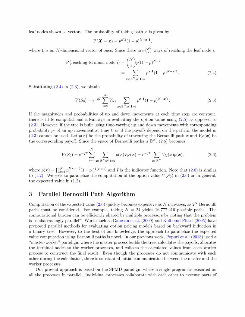
Figure 2.1: A two-step recombinant binomial tree with call option payoffs.

Starting with the current stock price in the market S0, a grid of possible future stock pricesSij is built using u and p. Algorithm 1 shows the procedure to build a binomial tree of simulatedfuture stock prices and calculate the payoffs at time T for a call option, for which, V (ST ) is givenby (2.1) at each j at time T . Therefore, VNj = max{SNj−K, 0}, j = 0, . . . , N , where Vij is V (Sij).Figure 2.1 shows a two-step recombinant binomial tree for a call option starting at the stock priceS with the stock price evolution and option payoffs.

In order to calculate the option value V (S0), the probabilities of reaching each of the leaf nodesof the tree must be calculated. These may be obtained from the probabilities of traversing eachof the Bernoulli paths of dimension N . Since we assume that p is constant from A2, all the pathswith the same number of up and down movements have the same probability of being traversed.The option value V (S0) is computed as the expectation of the payoffs discounted to the startingtime t = 0 at the annual interest rate q as

V (S0) = e−qTN∑i=0

p(i)VNi = e−qTN∑i=0

(N

i

)pi(1− p)N−iVNi, (2.3)

where p(i) =(Ni

)pi(1− p)N−i is the probability of traversing paths ending at leaf node i, whose

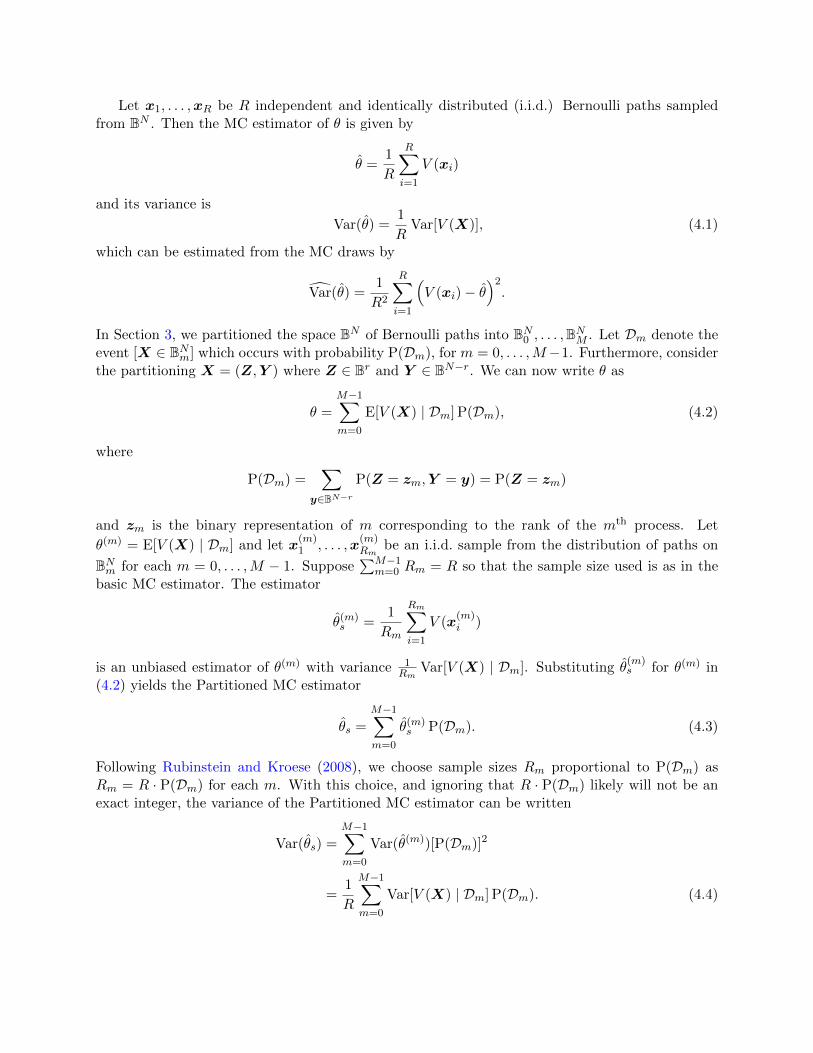
payoff is VNi.Let X = (X1, . . . , XN ) represent a Bernoulli path where each Xi ∼ Bernoulli(p) independently

for i = 1, . . . , N . Figure 2.2 shows the two-step binomial tree in Figure 2.1 with Bernoulli paths to

leaf nodes shown as vectors. The probability of taking path x is given by

P(X = x) = px′1(1− p)N−x′1,

where 1 is an N -dimensional vector of ones. Since there are(Ni

)ways of reaching the leaf node i,

P{reaching terminal node i} =

(N

i

)pi(1− p)N−i

=∑

x∈BN :x′1=i

px′1(1− p)N−x′1. (2.4)

Substituting (2.4) in (2.3), we obtain

V (S0) = e−qTN∑i=0

VNi∑

x∈BN :x′1=i

px′1(1− p)N−x′1. (2.5)

If the magnitudes and probabilities of up and down movements at each time step are constant,there is little computational advantage in evaluating the option value using (2.5) as opposed to(2.3). However, if the tree is built using time-varying up and down movements with correspondingprobability pt of an up movement at time t, or if the payoffs depend on the path x, the model in(2.3) cannot be used. Let p(x) be the probability of traversing the Bernoulli path x and VN (x) bethe corresponding payoff. Since the space of Bernoulli paths is BN , (2.5) becomes

V (S0) = e−qTN∑i=0

∑x∈BN :x′1=i

p(x)VN (x) = e−qT∑x∈BN

VN (x)p(x), (2.6)

where p(x) =∏Ni=1 p

I(xi=1)i (1− pi)I(xi=0) and I is the indicator function. Note that (2.6) is similar

to (1.2). We seek to parallelize the computation of the option value V (S0) in (2.6) or in general,the expected value in (1.2).

3 Parallel Bernoulli Path Algorithm

Computation of the expected value (2.6) quickly becomes expensive as N increases, as 2N Bernoullipaths must be considered. For example, taking N = 24 yields 16,777,216 possible paths. Thecomputational burden can be efficiently shared by multiple processors by noting that the problemis “embarrassingly parallel”. Works such as Ganesan et al. (2009) and Kolb and Pharr (2005) haveproposed parallel methods for evaluating option pricing models based on backward induction ina binary tree. However, to the best of our knowledge, the approach to parallelize the expectedvalue computation using Bernoulli paths is novel. In our previous work, Popuri et al. (2013) used a“master-worker” paradigm where the master process builds the tree, calculates the payoffs, allocatesthe terminal nodes to the worker processes, and collects the calculated values from each workerprocess to construct the final result. Even though the processes do not communicate with eachother during the calculation, there is substantial initial communication between the master and theworker processes.

Our present approach is based on the SPMD paradigm where a single program is executed onall the processes in parallel. Individual processes collaborate with each other to execute parts of

S

Sd

Su

Sd2; (0, 0)

Sud; (1, 0)Sdu; (0, 1)

Sd2; (1, 1)

(1− p)

p

p2

p(1− p)

(1−p)p

(1− p) 2

Figure 2.2: A two-step binomial tree with Bernoulli paths.

the program. It is not necessary for a master process to coordinate the workload in this problem;instead, each process can determine its share of the 2N paths to work on. This is possible using theunique rank assigned to each process. Each process computes a local expected value on its partitionof the sample space, and the final expected value is computed by summing across all processes. Thissummation is accomplished in the Message Passing Interface (MPI) framework through a “reduce”operation that coordinates communication between processes in an efficient way (Pacheco, 1997).

Suppose there are M parallel processes with ranks m = 0, . . . ,M −1; note that ranks tradition-ally start at 0 in the MPI framework. We assume that M ≤ N and that M is a power of 2. Letr = log2(M) so that the rank m of a process can be written with the r-digit binary representationm = zr−12r−1 + · · ·+ z121 + z020, where each zj ∈ B. Process m is assigned all paths x with prefix(zr−1, . . . , z1, z0); this set of 2N−r paths is denoted

BNm = {x ∈ BN : x1 = zr−1, . . . , xr−1 = z1, xr = z0}.

Note that the sets BNm form a partition of BN . Figure 3.1 shows a diagram of the mapping fromm to BNm. For each Bernoulli path x ∈ BNm, process m computes the probability of traversing thepath p(x) and the payoff value VN (x). The local expected value of the payoffs Vm on process m iscalculated as

Vm = e−qT∑x∈BN

m

p(x)VN (x). (3.1)

Finally, local expected values are summed to produce the final result

V (S0) =

M−1∑m=0

Vm; (3.2)

this is implemented by an MPI reduce operation to obtain the result on process 0. The computationof (3.2) requires 2N−r steps on 2r parallel processes rather than 2N steps on a single process, asrequired in the serial computation. The method can be extended to the case when M is not exactlya power of 2 if we are willing to forfeit perfect load balancing. For example, we can consider a

Figure 3.1: Process-Bernoulli path mapping

partition BN = BN0 ∪ · · · ∪BNK for some K >> M . Process 0 can handle BNm for m = 0,M, 2M, . . .,process 1 can handle BNm for m = 1,M + 1, 2M + 1, . . ., and so forth.

4 Monte Carlo Estimation and Variance Reduction

Recall that the number of Bernoulli paths in the set BN grows exponentially with N . When N be-comes large, it is infeasible to compute the expected value (2.6) exactly, even with a reasonably largenumber of processors. Monte Carlo (MC) estimation provides a way to approximate a complicatedexpected value without enumerating the entire sample space. In this section, we propose an MCmethod that uses the partitioning scheme from section 3 to approximate the result using M parallelprocesses. The mth process given the responsibility of drawing from BNm, for m = 0, . . . ,M − 1, sothat we effectively enumerate the first r = log2M steps of each path, and draw the rest throughMonte Carlo. This provides a reduction in variance over a basic MC estimator that uses the samenumber of draws.

Defineθ = E[V (X)] =

∑x∈BN

V (x)p(x),

where the suffix N in V (x) is dropped for notational convenience. The option value in (2.6) canbe written as V = e−qT θ. Given an estimate θ of θ, an estimate of V is V = e−qT θ, its varianceis Var(V ) = e−2qT Var(θ), and an estimate of the variance is Var(V ) = e−2qT Var(θ). Therefore, wewill focus on estimating θ for the remainder of this section.

Let x1, . . . ,xR be R independent and identically distributed (i.i.d.) Bernoulli paths sampledfrom BN . Then the MC estimator of θ is given by

θ =1

R

R∑i=1

V (xi)

and its variance is

Var(θ) =1

RVar[V (X)], (4.1)

which can be estimated from the MC draws by

Var(θ) =1

R2

R∑i=1

(V (xi)− θ

)2.

In Section 3, we partitioned the space BN of Bernoulli paths into BN0 , . . . ,BNM . Let Dm denote theevent [X ∈ BNm] which occurs with probability P(Dm), for m = 0, . . . ,M−1. Furthermore, considerthe partitioning X = (Z,Y ) where Z ∈ Br and Y ∈ BN−r. We can now write θ as

θ =M−1∑m=0

E[V (X) | Dm] P(Dm), (4.2)

where

P(Dm) =∑

y∈BN−r

P(Z = zm,Y = y) = P(Z = zm)

and zm is the binary representation of m corresponding to the rank of the mth process. Let

θ(m) = E[V (X) | Dm] and let x(m)1 , . . . ,x

(m)Rm

be an i.i.d. sample from the distribution of paths on

BNm for each m = 0, . . . ,M − 1. Suppose∑M−1

m=0 Rm = R so that the sample size used is as in thebasic MC estimator. The estimator

θ(m)s =

1

Rm

Rm∑i=1

V (x(m)i )

is an unbiased estimator of θ(m) with variance 1Rm

Var[V (X) | Dm]. Substituting θ(m)s for θ(m) in

(4.2) yields the Partitioned MC estimator

θs =M−1∑m=0

θ(m)s P(Dm). (4.3)

Following Rubinstein and Kroese (2008), we choose sample sizes Rm proportional to P(Dm) asRm = R · P(Dm) for each m. With this choice, and ignoring that R · P(Dm) likely will not be anexact integer, the variance of the Partitioned MC estimator can be written

Var(θs) =

M−1∑m=0

Var(θ(m))[P(Dm)]2

=1

R

M−1∑m=0

Var[V (X) | Dm] P(Dm). (4.4)

A corresponding variance estimator is

Var(θs) =1

R

M−1∑m=0

[1

Rm

Rm∑i=1

(V (x

(m)i )− θm

)2]

P(Dm)

=1

R2

M−1∑m=0

Rm∑i=1

(V (x

(m)i )− θm

)2.

To verify that θs gives a variance reduction over θ, the law of total variation gives

Var[V (X)] = ED Var[V (X) | D] + VarD E[V (X) | D] (4.5)

=

M−1∑m=0

Var[V (X) | Dm] P(Dm) + VarD E[V (X) | D]

= RVar(θs) + VarD E[V (X) | D], (4.6)

where the last equality is from (4.4). Substituting the left hand side in (4.6) in terms of Var(θ)from (4.1) and dividing both sides by R we get

Var(θ) = Var(θs) +VarD E[V (X) | D]

R. (4.7)

Note that VarD E[V (X) | D] = 0 if V (X) | D does not depend on the first r steps of the Bernoullipaths or when r ∈ {0, N}, that is, when the number of processes M ∈ {1, 2N}. When M = 1, thePartitioned MC method is same as the basic MC method and when M = N , it is same as the exactexpected value in (2.6). Since the payoff V (X) is assumed to depend on the entire path X, thesecond term in the right hand side of (4.7) is greater than 0 when 0 < r < N and, therefore, thePartitioned MC estimator in (4.3) typically yields strict reduction in the variance. We note thatthe variance reduction would be more pronounced when V (X) are heterogeneous across the Dmand homogeneous within each Dm.

Remark 1. An interesting variation of the Partitioned MC method is to reuse the same sample ofR draws from BN−r on all processes. Consider again the partitioning X = (Z,Y ), and suppose Z

and Y are independent. Let x(m)i = (zm,yi), where y1, . . . ,yR are i.i.d. draws from the distribution

of Y and z(m) = (z(m)r−1, . . . , z

(m)1 , z

(m)0 ) is the binary representation of m corresponding to the rank

of the mth process. Then an estimate for θ(m) is given by

θ(m) =1

R

R∑i=1

V (x(m)i ) (4.8)

and θ in (4.2) can be estimated unbiasedly by

θ =

M−1∑m=0

θ(m) P(Dm)

=1

R

R∑i=1

M−1∑m=0

V (x(m)i ) P(Dm)

=1

R

R∑i=1

EX|Y [V (Z,yi)]. (4.9)

The variance of this estimator is Var(θ) = 1R VarY EX|Y [V (X)] and an estimate of the variance

from the MC sample is

Var(θ) =1

R2

R∑i=1

(EX|Y [V (Z,yi)]− θ(m)

)2

=1

R2

R∑i=1

(M−1∑m=0

V (x(m)i ) P(Dm)− θ(m)

)2

.

We refer to θ as the Shared Sample MC estimator. Now, the variance of V (X) can be written as

Var[V (X)] = VarY E[V (X) | Y ] + EY Var[V (X) | Y ]

= RVar(θ) + EY Var[V (X) | Y ]. (4.10)

Substituting the left hand side in (4.10) in terms of Var(θ) from (4.1) and dividing both sides byR we get

Var(θ) = Var(θ) +EY Var[V (X) | Y ]

R. (4.11)

Again, the second term in the right hand side of the (4.11) is zero if and only if V (X) | Y doesnot depend on the first r steps of the Bernoulli paths, for 0 < r < N . Since we assume V (X)depends on the entire path X, Var(θ) is strictly less than Var(θ). The following result summarizesthe relationship among the variances of θ, θs, and θ.

Theorem 4.1. Suppose Rm = R for m = 0, . . . ,M − 1, 0 < r < N , and V (Zk,Y ) and V (Zl,Y )are positively correlated for all k, l ∈ {0, . . . ,M − 1}. Then Var(θs) ≤ Var(θ) ≤ Var(θ).

Proof. We have already shown that Var(θ) ≤ Var(θ). Now we have Var(θs) = 1R

∑M−1m=0 Var[V (X) |

Dm][P(Dm)]2, and from (4.9),

Var(θ) =1

RVarY

[M−1∑m=0

V (Zm,Y ) P(Dm)

]

=1

R

M−1∑m=0

VarY [V (Zm,Y )][P(Dm)]2 +1

R

∑∑k 6=l

Cov(V (Zk,Y ), V (Zl,Y )

)P(Dk) P(Dl)

= Var(θs) +1

R

∑∑k 6=l

Cov(V (Zk,Y ), V (Zl,Y )

)P(Dk) P(Dl)

≥ Var(θs).

5 Application to option pricing

We implemented the method described in Section 3 to value a put option using the R 3.2.2 andJulia 0.4.6 programming environments. Computations were run on the distributed cluster maya atthe UMBC High Performance Computing Facility (HPCF). The cluster maya has compute nodes,

each having two Intel E5-2650v2 Ivy Bridge (2.6 GHz, 20 MB cache) processors with 8 cores pernode, for a total of 16 cores per node. All nodes have 64 GB of main memory and are connectedby a quad-data rate InfiniBand interconnect. Open MPI 1.8.5 (Gabriel et al., 2004) was used asthe underlying implementation of the MPI framework.

R is a statistical computing environment that facilitates advanced data analysis, provides graph-ical capabilities and an interpreted high-level programming language (R Core Team, 2012). On topof the statistical, computational, and programmatic features available in the core R environment,additional capabilities are available through numerous packages which have been contributed bythe user community. The Rmpi (Yu, 2002) and pbdMPI (Ostrouchov et al., 2012) packages may beused to write MPI programs from R. Results shown in this section are based on Rmpi, but pbdMPI

performed similarly in our experience. The package Rcpp (Eddelbuettel and Francois, 2011) facili-tates integration of C++ code into R programs, which can substantially improve performance at thecost of an increased programming burden. We have not yet explored Rcpp in our implementation,but note its potential use.

Julia is a recently developed programming language that is gaining popularity in scientificcomputing, data analysis, and high performance computing (Bezanson et al., 2014). It is a compiledlanguage that uses the Low Level Virtual Machine Just-in-Time technology (Lattner and Adve,2004) to generate an optimized version of the source code compiled to the machine level. Julia

provides a number of computational and statistical capabilities, both in the core environment andthrough packages contributed by the user community. We have used the package MPI (Noack,2016) to run MPI programs in Julia. Integration with C++ is also possible in Julia throughpackages such as CxxWrap and Cpp, but we have not yet explored their use. Our implementationuses native Julia code with the MPI package. Because Julia is compiled into machine-level code,it is expected that a program written in Julia will perform better than an equivalent programwritten in R. Performance results later in this section confirm our hunch.

Listing 1 shows a snippet of our Julia implementation of the proposed parallelization method.Since the structure of our R and Julia implementations are similar, we do not show a similarlisting of our R code. In line 1 we load the MPI package. Since our implementation follows theSPMD paradigm, the same code runs on all the processes. The rank of the process on which thecode is being run is requested on line 5 and on line 6 the total number of processes in the MPIcommunicator is requested. As the while loop at line 11 shows, each process works on 2N−r outof the total 2N Bernoulli paths. Note the construction of the full Bernoulli path in line 13 byprepending the binary representation of the rank of the specific process on which the code is beingrun to the current (N−r)-dimensional Bernoulli path. The function call to calc path prob on line14 calculates the probability of traversing the Bernoulli path constructed in line 13. The functioncall to calc payoff on line 15 calculates the option payoff; their function definitions are not shownbecause they are independent of the parallelization method. Finally, on line 21, expected valuesfrom individual processes are summed together to obtain the final answer at process 0.

We take a put option as an example to illustrate our methodology. We set a strike price ofK = 10. Current price and volatility of the asset are S = 5 and σ = 0.30, respectively. Risk-freeinterest rate is q = 6% and time to maturity T is one year. Tables 5.1(a) and 5.2(a) show the wallclock runtimes of our R and Julia implementations, respectively, for problem sizes N = 20, 24, 28,and 32. While both the implementations scale well with the number of processes M , the Julia

implementation is roughly 10 times faster than R. Our program for N = 32 on a single process(M = 1) resulted in an overflow in our loop that computes the expected value since 231 − 1 is the

1 import MPI

2 .

3 MPI.Init()

4 comm = MPI.COMM_WORLD

5 id = MPI.Comm_rank(comm)

6 M = MPI.Comm_size(comm)

7 .

8 r = log2(M)

9 l_n = convert(Int64 , 2^(N-r))

10 .

11 while i < l_n

12 node = i

13 path = cat(2, integer_base_b(id, 2, r), integer_base_b(node , 2, N-r))

14 p_vt = calc_path_prob(path , probs)

15 vt = calc_payoff(S, K, u, d, opt_type , path)

16 v += p_vt*vt

17 i += 1

18 end

19 .

20 v = exp(-q*T)*v

21 reduced_v = MPI.Reduce(v, MPI.SUM , 0, comm)

Listing 1: A Julia implementation of the parallel Bernoulli path algorithm.

maximum integer value that can be stored in R. As a result, the runtime for this particular caseis recorded as N/A in Table 5.1(a). If TM is the runtime taken for M number of processes, thespeedup SM and efficiency EM for M are defined as T1/TM and SM/M respectively. If the programscales up perfectly to M processes, ideal values SM = M and EM = 1 are obtained. These numbersindicate the scalability of the program. Since our R program did not run on a single process forN = 32, we take the speedup for this case to be 2·T2/TM , M = 2, . . . , 64 and for M = 1 and M = 2,the speedups are taken to be 1 and 2 respectively. Tables 5.1(b) and 5.2(b) show the speedupsand Tables 5.1(c) and 5.2(c) show the efficiency numbers of our R and Julia implementations,respectively. The plots in Figure 5.1 visualize the speedup and efficiency numbers in Tables 5.1(b)and 5.1(c), respectively, and Figure 5.2 shows the corresponding plots from Table 5.2. These plotsvisually confirm our conjecture that Julia is more efficient than R for our problem. Note that for afixed problem size, there is a reduced advantage in the speedup beyond a certain number of tasks.This is because the overhead of coordinating the tasks begins to dominate the time spent doinguseful calculations; see Pacheco (1997) for more details.

We implemented the Monte Carlo estimation methods described in Section 4 for two typesof path-dependent options (Hull, 2003): Asian and Look-back options. In an Asian option, theasset price ST at the time of maturity is replaced in the option payoff function with the arithmeticaverage of {St : t = 1, . . . , N}. Therefore, in the binomial tree model, the payoff for an Asian putoption is given by

V (x) = max{K − S∗, 0}, (5.1)

where S∗ = 1N

∑Nt=1 St(x), St(x) is the asset value at time t followed on the Bernoulli path x.

In a Look-back option, either the strike price K or the asset price ST at the time of maturity arereplaced in the payoff function by the maximum or minimum of {St} respectively. Here we consider

(a) (b)

Figure 5.1: (a) Speedup and (b) Efficiency in R.

a Fixed Look-back put option, whose payoff is given by

V (x) = max{K − S∗, 0},

where S∗ = min{St(x) : t = 1, . . . , N}. We implemented the basic MC estimate given in section4 for the Asian and Fixed Look-back put options using the binomial tree model with size N tostudy the convergence of the estimates to the exact expected value (2.6). We further implementedPartitioned and Shared Sample MC from section 4 to study the variance reduction property. Table5.3 shows basic MC estimates and corresponding variance estimates of an Asian put option anda Fixed Look-back put option with parameters K = 100, S = 20, q = 6%, σ = 3.0, and T = 1,using the binomial model with tree size N = 32. Option values calculated by exact enumerationwere 82.115 for the Asian put options and 93.196 for the Fixed Look-back put option. The samplesize used for the MC estimation is increased from 29 to 216, which is less than 0.01% of the totalnumber of paths. As can be seen from Table 5.3, MC estimates for both the options converge totheir respective exact values. Also, as expected, the variance estimates decrease with increasingsample size R. Table 5.4 shows the Partitioned MC estimates Vs for both the Asian and FixedLook-back put options and corresponding variance estimates, using a total sample size of R = 1024and varying the number of processes between 1 to 64. Note that as the number of processes increase,the sample size per process Rm decreases. The estimates shown in Table 5.4 are averaged over 1000repetitions. As expected, Table 5.3 shows that variance estimates of the Partitioned MC estimatorare mostly smaller than the corresponding basic MC estimator for R = 1024. Table 5.5 showsthe comparison of variance estimates between the Partitioned and Shared Sample MC estimatesfor the Asian put option with N = 32, R = Rm = 1024, and m = 0, . . . ,M − 1. Shared SampleMC estimates V and corresponding variance estimates were calculated using the expressions givenin section 4. Again, the estimates in Table 5.5 are averaged over 1000 repetitions. The resultsshow that if R = Rm, and m = 0, . . . ,M − 1, the Partitioned MC method reduces the varianceof the estimator more than the Shared Sample method does, as expected from Theorem 4.1. Thecondition on the covariance between V (zk,y) and V (zl,y) for all k, l ∈ {0, . . . ,M − 1} where k 6= lis satisfied for the options considered here.

Table 5.1: Runtime for different number of time steps for R implementation. For M = 1, N = 32, since our program failed torun because of integer overflow, runtime is shown as N/A.

(a) Wall clock time in HH:MM:SSN M = 1 2 4 8 16 32 64

20 00:00:68 00:00:37 00:00:24 00:00:14 00:00:07 00:00:04 00:00:0224 00:19:41 00:10:39 00:07:00 00:04:02 00:02:04 00:01:05 00:00:3228 05:45:57 03:04:34 02:08:18 01:09:07 00:36:25 00:18:17 00:09:1532 N/A 52:16:13 36:15:16 20:26:59 11:04:18 05:21:38 02:41:57

(b) Observed speedup SMN M = 1 2 4 8 16 32 64

20 1.00 1.81 2.79 4.92 3.38 6.61 12.8024 1.00 1.85 2.81 4.88 9.30 18.58 37.2228 1.00 1.87 2.69 5.00 9.49 18.90 37.3832 N/A 2.00 2.88 5.11 9.44 19.50 38.72

(c) Observed efficiency EMN M = 1 2 4 8 16 32 64

20 1.00 0.90 0.70 0.62 0.21 0.21 0.2024 1.00 0.92 0.70 0.61 0.58 0.58 0.5828 1.00 0.94 0.67 0.62 0.60 0.60 0.5832 N/A 1.00 0.72 0.64 0.59 0.61 0.60

Table 5.2: Runtime for different number of time steps for Julia implementation.

(a) Wall clock time in HH:MM:SSN M = 1 2 4 8 16 32 64

20 00:00:07 00:00:05 00:00:02 00:00:01 00:00:01 00:00:01 00:00:0124 00:02:23 00:01:15 00:00:42 00:00:22 00:00:11 00:00:06 00:00:0328 00:40:08 00:21:05 00:11:02 00:05:56 00:03:07 00:01:34 00:00:5132 11:59:54 06:23:01 03:24:58 01:46:06 00:53:41 00:27:18 00:13:38

(b) Observed speedup SMN M = 1 2 4 8 16 32 64

20 1.00 1.80 3.16 6.18 11.10 17.65 25.0524 1.00 1.91 3.36 6.37 13.02 24.76 47.7928 1.00 1.90 3.64 6.76 12.90 25.71 47.0632 1.00 1.88 3.52 6.76 13.44 26.37 52.58

(c) Observed efficiency EMN M = 1 2 4 8 16 32 64

20 1.00 0.90 0.79 0.77 0.69 0.55 0.3924 1.00 0.95 0.84 0.79 0.81 0.77 0.7528 1.00 0.95 0.91 0.86 0.81 0.80 0.7332 1.00 0.94 0.88 0.85 0.84 0.82 0.82

(a) (b)

Figure 5.2: (a) Speedup and (b) Efficiency in Julia.

Table 5.3: Monte Carlo estimates and corresponding variance estimates for Asian and Fixed Look-back put options with N = 32.Exact value of the Asian option is 82.115 and the Look-back option is 93.196.

Option Estimate R = 29 210 211 212 213 214 215 216

Asian V 82.857 82.514 83.425 83.181 82.821 82.615 82.566 82.524

Var(V ) 0.735 0.362 0.179 0.095 0.050 0.022 0.011 0.006

Look-back V 93.156 93.237 93.312 93.324 93.262 93.236 93.234 93.222

Var(V ) 0.022 0.009 0.005 0.002 0.001 <0.001 <0.001 <0.001

Table 5.4: Partitioned Monte Carlo estimates and corresponding variance estimates for Asian and Fixed Look-back put optionswith N = 32 and R = 210.

Option Estimate M = 1 2 4 8 16 32 64Rm = 210 29 28 27 26 25 24

Asian Vs 82.077 82.217 82.101 82.232 81.936 82.296 82.165

Var(Vs) 0.367 0.332 0.315 0.272 0.263 0.212 0.194

Look-back Vs 93.196 93.201 93.171 93.197 93.187 93.216 93.205

Var(Vs) 0.010 0.009 0.008 0.008 0.008 0.007 0.007

Table 5.5: Comparison of the variance estimates from the Partitioned and Shared Sample Monte Carlo methods with N = 32and R = 1024 for Asian put option.

Method Estimate M = 1 2 4 8 16 32 64

Partitioned MC Vs 82.201 82.160 82.101 82.127 82.109 82.120 82.108

Var(Vs) 0.367 0.220 0.062 0.027 0.005 0.005 0.002

Shared Sample MC V 82.113 82.112 82.120 82.093 82.102 82.124 82.108

Var(V ) 0.373 0.305 0.267 0.203 0.170 0.142 0.123

6 Concluding Remarks

We have proposed a novel method to transform the computation of the expected value in a recom-binant binomial tree into an embarrassingly parallel problem by mapping the Bernoulli paths in thetree to the processes on a multiprocessor computer. We also proposed a Monte Carlo estimationmethod which takes advantage of this partitioning. The proposed methods were implemented bothin R and Julia, and were applied to value path-dependent European options. Numerical resultsverify the convergence of the proposed Monte Carlo method and variance reduction with respectto basic Monte Carlo estimation. Performance results indicate that the Julia implementation wassignificantly faster and more efficient than the R implementation, likely because of the superiorhandling of loops and the compilation to machine-level code.

Acknowledgments

The first author acknowledges financial support from the UMBC High Performance ComputingFacility (HPCF) at the University of Maryland, Baltimore County (UMBC). The hardware usedin the computational studies is part of HPCF. The facility is supported by the U.S. NationalScience Foundation through the MRI program (grant no. CNS–0821258 and CNS–1228778) andthe SCREMS program (grant no. DMS–0821311), with additional substantial support from theUniversity of Maryland, Baltimore County (UMBC). See hpcf.umbc.edu for more information onHPCF and the projects using its resources.

References

J. Bezanson, A. Edelman, S. Karpinski, and V. B. Shah. Julia: A fresh approach to numericalcomputing, 2014. arXiv:1411.1607.

John C. Cox, Stephen A. Ross, and Mark Rubinstein. Option pricing: A simplified approach. Jour-nal of Financial Economics, 7(3):229–263, 1979. ISSN 0304-405X. doi: http://dx.doi.org/10.1016/0304-405X(79)90015-1. URL http://www.sciencedirect.com/science/article/pii/

0304405X79900151.

Dirk Eddelbuettel and Romain Francois. Rcpp: Seamless R and C++ integration. Journal ofStatistical Software, 40(8):1–18, 2011. URL http://www.jstatsoft.org/v40/i08/.

Ian Foster. Designing and Building Parallel Programs: Concepts and Tools for Parallel SoftwareEngineering. Addison-Wesley, 1995.

Edgar Gabriel, Graham E. Fagg, George Bosilca, Thara Angskun, Jack J. Dongarra, Jeffrey M.Squyres, Vishal Sahay, Prabhanjan Kambadur, Brian Barrett, Andrew Lumsdaine, Ralph H.Castain, David J. Daniel, Richard L. Graham, and Timothy S. Woodall. Open MPI: Goals,Concept, and Design of a Next Generation MPI Implementation. In Proceedings, 11th EuropeanPVM/MPI Users Group Meeting, Budapest, Hungary, Sept 2004.

Narayan Ganesan, Roger D. Chamberlain, and Jeremy Buhler. Acceleration of binomial optionspricing via parallelizing along time-axis on a GPU. Proc. of Symp. on Application Acceleratorsin High Performance Computing, 2009.

Mina Hosseini, Nagaraj K. Neerchal, and Ann L. Gruber-Baldini. Statistical modeling of sub-ject and proxy observations using weighted GEE. In JSM Proceedings, Section on Statistics inEpidemiology. Alexandria, VA: American Statistical Association, pages 1101–1111, 2016.

John C. Hull. Options, Futures, And Other Derivatives. Prentice Hall, 2003.

C. Kolb and M. Pharr. Option pricing on the GPU in GPU Gems 2. Addison-Wesley, 2005.

Chris Lattner and Vikram Adve. LLVM: A Compilation Framework for Lifelong Program Analysis& Transformation. In Proceedings of the 2004 International Symposium on Code Generation andOptimization (CGO’04), Palo Alto, California, Mar 2004.

Roderick J. A. Little. Pattern-mixture models for multivariate incomplete data. Journal of theAmerican Statistical Association, 88(421):125–134, 1993.

Andreas Noack. Julia - MPI package. https://github.com/JuliaParallel/MPI.jl, 2016.

G. Ostrouchov, W.-C. Chen, D. Schmidt, and P. Patel. Programming with big data in R, 2012.URL http://r-pbd.org/.

Peter S. Pacheco. Parallel Programming with MPI. Morgan Kaufmann, 1997.

Sai K. Popuri, Andrew M. Raim, Nagaraj K Neerchal, and Matthias K. Gobbert. An implementa-tion of binomial method of option pricing using parallel computing. Technical Report TechnicalReport HPCF–2013–1, UMBC High Performance Computing Facility, University of Maryland,Baltimore County, 2013. URL http://userpages.umbc.edu/~gobbert/papers/PopuriEtAl_

Binomial.pdf.

R Core Team. R: A Language and Environment for Statistical Computing. R Foundation forStatistical Computing, Vienna, Austria, 2012. URL http://www.r-project.org. ISBN 3-900051-07-0.

Reuven Y. Rubinstein and Dirk P. Kroese. Simulation and the Monte Carlo Method. John Wileyand Sons, 2008.

Rudiger Seydel. Tools for Computational Finance. Springer, 2003.

Hao Yu. Rmpi: Parallel statistical computing in R. R News, 2(2):10–14, 2002. URL http:

//cran.r-project.org/doc/Rnews/Rnews_2002-2.pdf.