parallel implementation of eigenfaces for face · pdf file · 2014-08-10parallel...
TRANSCRIPT

Parallel Implementation of Eigenfaces for Face
Recognition on CUDA
Dissertation
Submitted in partial fulfillment of the requirement for the degree of
Master of Technology in Computer Engineering
By
Manik R. Kawale
MIS No: 121222015
Under the guidance of
Dr. Vandana Inamdar
Department of Computer Engineering and Information Technology
College of Engineering, Pune
Pune – 411005
June, 2014

DEPARTMENT OF COMPUTER ENGINEERING AND
INFORMATION TECHNOLOGY,
COLLEGE OF ENGINEERING, PUNE
CERTIFICATE
This is to certify that the dissertation titled
Parallel Implementation of Eigenfaces for Face Recognition on CUDA
has been successfully completed
By
Manik R. Kawale
MIS No: 121222015
and is approved for the partial fulfillment of the requirements for the degree of
Master of Technology, Computer Engineering
Dr. Vandana Inamdar
Project Guide,
Department of Computer Engineering
and Information Technology,
College of Engineering, Pune,
Shivaji Nagar, Pune-411005.
Dr. J. V. Aghav
Head,
Department of Computer Engineering
and Information Technology,
College of Engineering, Pune,
Shivaji Nagar, Pune-411005.
June 2014

ii
Acknowledgments
I express my sincere gratitude towards my guide Dr. Vandana Inamdar for her constant help,
encouragement and inspiration throughout the project work. Without her invaluable guidance,
this work would never have been a successful one. I am extremely thankful to Dr. J. V. Aghav
for providing me infrastructural facilities to work in, without which this work would not have
been possible. Last but not least, I would like to thank my family and friends, who have been a
source of encouragement and inspiration throughout the duration of the project.
Manik R. Kawale
College of Engineering, Pune

iii
Abstract
Face has significant role in identifying a person. Face recognition has many real world
applications including surveillance and authentication. Due to complex and multidimensional
structure of face it requires huge computations therefore fast face recognition is required. One of
the most successful template based techniques for face recognition is Principal Component
Analysis (PCA) which is generally known as eigenface approach. It suffers from the
disadvantage of higher computation cost, despite its better recognition rate. With the increase in
number of images in training database and also the resolution of images, the computational cost
also increases.
Graphics Processing Unit (GPU) is the solution for fast and efficient computation. GPUs
have massively parallel multi-threaded environment. With the use of GPU's parallel
environment, a problem can be solved in parallel with much less time. NVIDIA has released a
parallel programming framework CUDA (Compute Unified Device Architecture), which
supports popular programming languages with CUDA extension for GPU programming.
A parallel version of eigenface approach for face recognition is developed using CUDA
framework.

iv
Contents
Certificate i
Acknowledgement ii
Abstract iii
List of Figures vi
List of Tables vii
1. Introduction 1
1.1 Biometric 1
1.2 Introduction to Face Recognition 1
1.3 Introduction to Parallel Computing 3
1.4 GPU 5
1.5 CUDA 7
2 Literature Survey 11
2.1 Eigenface Approach 11
2.2 Related Work 13
3 Problem Statement 14
3.1 Motivation 14
3.2 Problem Statement 14
3.3 Objective 14
4 Implementation 15
4.1 Parallel Implementation 15

v
5 Result 20
6 Conclusion and Future Work 25
5.1 Conclusion 25
5.2 Future Work 25
Bibliography

vi
List of Figures
1.1 Steps involved in Face recognition 2
1.2 Modern GPU Architecture 6
1.3 Execution of CUDA Program 7
2.1 Sample Eigenfaces 11
4.1 System Architecture 16
5.1 Speedup of Individual modules 23
5.2 Training Phase Speedup 24
5.3 Transfer Time 24

vii
List of Tables
5.1 System Specification 20
5.2 Execution Time & Speedup of Normalization Module 21
5.3 Execution Time & Speedup of Covariance Module 21
5.4 Execution Time & Speedup of Jacobi Module 21
5.5 Execution Time & Speedup of Eigenface Module 22
5.6 Execution Time & Speedup of Weights Module 22
5.7 Execution Time & Speedup of Recognition Module 22
5.8 Execution Time & Speedup of Training Phase 23

1
Chapter 1
Introduction
1.1 Biometric
The world “biometrics” came from Greek words “bio” means life and “metrics” means to
measure. Biometric is the process of identification of humans with the use of measurable
biological characteristics or trait. In computer science, biometric is used for authentication and
access control.
User authentication can be done in three ways [6]:
Something you know (password or pin)
Something you have (key or id card)
Something you are i.e. biometrics (your face, voice, fingerprint or DNA)
Advantages of biometrics over other authentication techniques are that they cannot be
forgotten or lost. Also, biometrics characters are unique to individual humans so they are more
difficult to fake. There are many types of biometrics systems including face recognition,
fingerprint recognition, iris recognition etc.
1.2 Introduction to Face Recognition
Face recognition is one of the important methods of biometric identification. Developing a face
recognition model continues to be an extremely fascinating field for many researchers mainly
because of its many real world applications like criminal identification, user authentication,
security systems and surveillance systems. However, due to its complex and multidimensional
structure, it is difficult to develop a face recognition model.
The face recognition process basically involves four steps image acquisition, image pre-
processing, feature extraction and classification as shown in figure 1.1.

2
Figure 1.1 Steps involved in Face Recognition
Image acquisition is the first step in face recognition which involves reading an input image from
disk or camera and locating face in that image. In image pre-processing step, image enhancement
techniques are applied on input image like histogram equalization, sharpening and smoothing.
Generally a combination of several image enhancement techniques is applied to get the best
result.
In feature extraction step, a feature vector unique to the image is generated by analyzing the face
and a template is created. In the final step, a test image is classified into either one of the known
face or unknown face using classification techniques.
The amount of computation and memory required in these face recognition steps is mainly
affected by the approach used for face representation, that is, how to model a face. Depending
upon the face representation approach, face recognition algorithms are classified into template
based, feature based and appearance based.
i. Template based approach
In a most simple template based approach for face representation, a single template, i.e.
Image
Acquisition
Image
Preprocessing
Template
Generation
Test Image Classification Result
Template
Database

3
an array of intensities of face image, is used. Multiple templates of each face may be used
in a complex method of template based approach where each template represents
different viewpoint. Simplicity is the advantage of template based approach, but it has a
major disadvantage of very huge requirements and inefficient matching.
ii. Feature based approach
Feature based approach uses facial features like relative position and/or size of eyes, nose
and jaw to represent faces. To recognize a test face, same set of features are extracted
from test image as earlier and are matched to precompiled features. The advantages of
feature based approach are very little memory requirements and faster recognition speed.
But in practical, it is very difficult to implement perfect feature extraction technique.
iii. Appearance based approach
Appearance based approach is somewhat similar to template based approach. In this
approach a face image is projected onto a linear subspace which has much lower
dimensions compared to original image dimensions. This low dimensional subspace has
to be precompiled by applying Principal Component Analysis (PCA) on training face
image set. Appearance based approach requires very less memory as compared to
template based approach and, also, it has fast recognition rate. The major drawback of
appearance based approach is that it has high computation cost.
As compared to template based and feature based approach, appearance based approach is simple
and efficient except its high computation cost. If some way of lowering the computational cost is
developed then appearance based approach is a good practical approach for face recognition.
One way of doing this is to use the parallel environment of GPU. GPU can process huge amount
of data by executing same instruction concurrently on a sub-set of data. So with GPU a faster
appearance based face recognition can be implemented.
1.3 Introduction to parallel computing
Parallel computing has attracted many of the researchers in recent years, who are trying to
increase the performance of various applications and algorithms with the use of parallel
computing techniques. Parallel computing is being used in a number of scientific and industrial

4
applications from nuclear science to medical diagnosis. In computer science, it is being used for
image processing, graphics rendering, data mining and various other applications. All these
applications require large computation. Due to increase in computing power and storage of
computers, demand for fast processing in increased.
In general, parallel computing is the use of multiple computing resources simultaneously to solve
a problem. It aims to solve a problem by dividing the problem into discrete sub-problems that
can be solved concurrently. Instructions from each sub-problem executes concurrently on
different processor. Parallel algorithms are designed to effectively use most of the computing
resources of a system. A large no of real world applications requires high computation, thus it
requires the exploration of possible parallelism in the application which gives higher
performance.
Parallel computing models are generally classified into four groups based on the number of
instruction and data streams, as following:
i. SISD
This group of computers has single processor that executes instructions one after another.
SISD computers, also called sequential, are not capable of performing parallel computing
on their own.
ii. MISD
This group of computers has multiple processors. Each processor executes different set of
instructions on the same set of data. There are not much MISD computers, because the
problems that can be solved by MISD computer are uncommon.
iii. SIMD
This group of computers has multiple processors that performs same set of instructions,
but each processor has different set of input data, thus employing data parallelism This is
the most important class of parallel computing.
iv. MIMD
This group of computers has multiple processors that perform its own set of instructions.
Each processor also has different set of data. This kind of system is important when
different algorithms have to be executed on different sets of data.
5
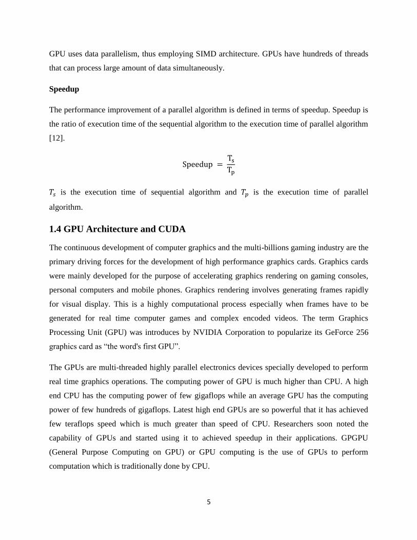
GPU uses data parallelism, thus employing SIMD architecture. GPUs have hundreds of threads
that can process large amount of data simultaneously.
Speedup
The performance improvement of a parallel algorithm is defined in terms of speedup. Speedup is
the ratio of execution time of the sequential algorithm to the execution time of parallel algorithm
[12].
is the execution time of sequential algorithm and is the execution time of parallel
algorithm.
1.4 GPU Architecture and CUDA
The continuous development of computer graphics and the multi-billions gaming industry are the
primary driving forces for the development of high performance graphics cards. Graphics cards
were mainly developed for the purpose of accelerating graphics rendering on gaming consoles,
personal computers and mobile phones. Graphics rendering involves generating frames rapidly
for visual display. This is a highly computational process especially when frames have to be
generated for real time computer games and complex encoded videos. The term Graphics
Processing Unit (GPU) was introduces by NVIDIA Corporation to popularize its GeForce 256
graphics card as “the word's first GPU”.
The GPUs are multi-threaded highly parallel electronics devices specially developed to perform
real time graphics operations. The computing power of GPU is much higher than CPU. A high
end CPU has the computing power of few gigaflops while an average GPU has the computing
power of few hundreds of gigaflops. Latest high end GPUs are so powerful that it has achieved
few teraflops speed which is much greater than speed of CPU. Researchers soon noted the
capability of GPUs and started using it to achieved speedup in their applications. GPGPU
(General Purpose Computing on GPU) or GPU computing is the use of GPUs to perform
computation which is traditionally done by CPU.

6
CPUs have few cores that are optimized to perform sequential computing while GPUs have
thousands of cores which are specially designed for parallel processing. So a significant speedup
can be achieved by executing high computational work on GPU while rest of code in CPU.
Researchers have used GPU computing to accelerate various engineering and scientific
problems.
1.4.1 GPU Architecture
Figure 1.2 Modern GPU Architecture
A CUDA capable GPU consists of a set of streaming multiprocessors (SMs) as shown in figure
1.2. Each streaming multiprocessor has a number of processor cores. A streaming multiprocessor
processor core is known as streaming processor (SP). The number of streaming processors each
streaming multiprocessor contains depends on the GPU. Generally, in modern GPU each
streaming multiprocessor contains 32 streaming processors. So if a GPU has 512 cores that mean
it contains 16 streaming multiprocessors each containing 32 cores or streaming processors.

7
The programs running on GPU are independent of architectural differences which make GPU
programming scalable.
1.5 CUDA
Compute Unified Device Architecture (CUDA) is a parallel computing platform and
programming model developed by NVIDIA which is implemented on GPUs they manufacture. It
is a proprietary technology of NVIDIA. Before CUDA, computer graphics programmers were
using shader languages such as GLSL2. Shading language deals with the computer graphics
domain. So it was mandatory to learn some computer graphics terminology before developing
GPU programs. CUDA provides its own libraries, compilers and supports popular programming
languages like C, C++ and FORTRAN. Other third party wrappers are available for other
languages like Java and Python.
1.5.1 CUDA Program Structure
A CUDA program consists of two kinds of codes, one is the standard C code which runs serially
on the CPU, and the other is the extended C code which executes parallely on the GPU. In the
CUDA programming model, CPU is also refers to a host, while GPU refers to a device. Figure
1.3 shows the executions of a CUDA program.
Figure 1.3 Execution of a CUDA Program
GPU parallel kernel
KernalA<<<dimGrid,dimBlock>>>(args);
GPU parallel kernel KernalB<<<dimGrid,dimBlock>>>(args);
Host Serial Code
Host Serial Code

8
Generally, a CUDA program starts execution from the host side code, which runs serially. When
it reaches a device code, such as a kernel, the program starts to execute in parallel GPU. When
the parallel execution of the device code completes, the program returns the control to CPU. This
allows the concurrent execution of serial code on CPU and parallel device code of GPU,
especially when there is no data dependence between host code and device code [14].
CUDA programs are compiled by nvcc compiler provided by NVIDIA. It first separates the host
and device code from a CUDA program. The host code is then further compiled by a standard C
compiler like gcc. While nvcc further compiles the device code as well to make it able to execute
in parallel on GPU. The device code uses C syntax with a few extensions, i.e. keywords, which
allows nvcc compiler to split the device code from the whole program. The main differences
between host code and device code are their execution pattern and memory structure. The device
code is executed in parallel rather than in serial, it also uses a variety of memory types within the
GPU.
The parallel execution code and different memory types are specified by the extended CUDA
keywords. CUDA introduced two additional functions, kernel function and device function. The
kernel function with the __global__ qualifier generates multiple threads running on GPU, and the
device function with the __device__ qualifier only executes on a single thread. The execution of
a parallel CUDA program is a two level hierarchal structure. The launch of a kernel invokes a
grid which consists of several blocks and each block includes a large number of threads. The
structure of the grid and blocks is determined at the time of invocation of a kernel. To specify
dimension of grid and its blocks, kernel invocation uses <<<gridDim, blockDim>>> syntax.
1.5.2 CUDA Memory Types
GPU has its own memory, and there are many types of memories in GPU’s memory hierarchy.
Variables in the GPU side cannot be used in the CPU side, nor can the variables on CPU side to
be used on GPU side. Therefore, there must be explicit transfer of data between host and device.
Two interrelated buffers which reside on GPU and CPU separately are usually allocated by a
CUDA program. The host buffer stores the initial data. In order to make it available on the GPU
side for parallel operation on it during the invocation of kernel, this buffer on the CPU should
copy data to its corresponding buffer on the GPU. When the execution of the kernel completes
9
and the output data is generated, the buffer on the GPU should also transfer the outcome to its
corresponding buffer on the CPU. This process is realised by the CUDA runtime function
cudaMemcpy. Allocation of a buffer on a GPU is done by cudaMalloc, this buffer is dynamically
allocated so it can be freed up after use by cudaFree.
There are four memory types in CUDA, Global Memor, Shared Memory, Constant Memory and
Registers. Each has different access latency and bandwidth. To achieve best performance gain,
each memory type should be used efficiently. Different types of variable are specified by
additional CUDA keywords. The scope of variables refers to the threads that can access the
variable. This is caused by the design of two level hierarchy structures of threads in CUDA
programming model. A variable can either be accessed from a single thread, or it can be accessed
from a block, or it can be accessed from the whole grid.
Global Memory: Global memory has much higher latency and lower bandwidth
compared to other memory spaces on GPU, although compared to CPU memory the
bandwidth of global memory is many times higher. Global variables reside in global
memory. Global variables are specified by an optional __device__ qualifier. It is created
and operated in the host code by invoking the CUDA runtime APIs such as cudaMalloc
and cudaMemcpy. Global variables have the scope of the entire grid, and their lifetime is
across the entire program. The value of global variables is maintained throughout
multiple invocations of different kernel functions. Global variables are particularly used
to pass data between different kernel executions.
Shared Memory: Global memory exists in DRAM on a GPU. By contrast, Shared
memory is on chip memory which is much like a cache manipulated by user. Each SM
has its own shared memory that is evenly partitioned in terms of the number of blocks on
the SM and assigned to these blocks during runtime. Therefore, access to shared memory
is much faster than global memory. Shared memory also consists of several memory
banks which allow it to be accessed simultaneously by threads. This feature of shared
memory yields the result that its bandwidth is several times as high as that of a single
bank. Shared variables specified by __shared__ qualifier reside on shared memory.
Shared variables have the scope of a block. Shared variables have the lifetime of the
block.

10
Constant Memory: Similar to global memory, constant memory space is in DRAM and
can be both read and written in the host code. However, constant memory has much
faster access speed than global memory. In the host code, constant memory only provides
read-only access. Constant variables are specified by __constant__ qualifier, it must be
declared outside any function body.
Registers: Registers are another kind of on chip memory with extremely low latency.
Each SM has a set of registers that are assigned to threads. Unlike shared memory that is
owned by all threads in a block, registers are exclusively owned by each thread. Access
to shared memory can be highly parallel due to its multiple banks, also registers can also
be highly parallel because each thread has its unique registers. Variables placed into
registers are part of automatic variables which refer to variables declared within a kernel
or device function without any qualifier. The scope of variables is within individual
thread. As the number of registers is limited, only a few automatic variables will be
stored in registers. The remaining variables will reside in local memory space with the
same high latency and low bandwidth as global memory.

11
Chapter 2
Literature Survey
2.1 Eigenface Approach
Eigenfaces can be extracted out of an image by performing Principle Component Analysis
(PCA) and Sirovich and Kirby are among the first researchers to utilize this approach [2]. They
showed that any particular face can be represented along the eigenpicture coordinate space
utilizing a much smaller amount of memory. Also a face can be reconstructed utilizing a small
collection of eigenpictures and their corresponding projections, called coefficients, along each
eigenpicture.
Principal Component Analysis (PCA) is a mathematical procedure invented by Karl Pearson [3].
It is used to reduce the dimensionality of a data set consisting of a large number of unrelated
variables i.e. having redundancy. PCA gives a new set of variables called Principal Components.
Principal components retains as much as possible of the variation present in the data set and are
stored in decreasing order of significance, which allows even further reduction by only utilizing
the top few components. Applying PCA and producing the eigenfaces reduces the number of
dimensions that need to be explored by the face classifier.
Figure 2.1 Sample Eigenfaces

12
Eigenfaces are called so due to the fact that they look like ghostly faces as seen in figure 2.1. The
eigenfaces define a feature space or face space, where the dimensionality of this new space is
dramatically reduced from the original space. Having this reduced spaces saves in complexity of
the classification and the storage of these images.
The mean face of the faces in training set is given in equation below, which is calculated by
averaging each pixel of all the images.
(
)∑
In above equation, M represents the number of training images and is a training image of size
N×N.
The mean adjusted image is given by following equation
The covariance matrix, denoted C, is defined as
∑
Using PCA we can obtain a set of M eigenvectors and their corresponding eigenvalues of
the covariance matrix C. Each of this M eigenvector corresponds to an eigenface. Only top few
eigenvectors are selected thus reducing the eigenface space.
We can calculate the eigenface components of an image by projecting it onto the mean face
space. Each eigenface is given by the sum of its corresponding eigenvector scaled by each input
face image vector.
where is the mean centered image and is the ith
eigenvector.
Finally, we calculate the reconstructed image of the projection.

13
∑
Now we have all the calculation, we can utilize the reconstructed image and the mean centered
image to determine whether the image is similar to a face or not. Since we only select the
eigenfaces with the higher eigenvalues we have a smaller space to compare and classify the
images with. This is the benefit in using eigenfaces.
2.2 Related work
Wendy S. et al. concluded in their analysis that using standard PCA algorithm, a strong
recognition rate can be achieved [5].
Due to its simplicity and good recognition rate researchers have tried to reduce the time
complexity of eigenfaces to speed up the process. Patrik Kamencay et al. designed an improvd
face recognition algorithm using graph based segmentation algorithm [7]. Although they
improved recognition rate but time requirements were not majorly minimized.
Wlodzimierz M. Baranski et al. used BST to reduce the time [8]. They achieved a slightly higher
recognition rate but the speed up achievement was below 2x. Neeraja and Ekta Walia used fuzzy
feature extraction along with PCA for accelerating the process [9]. Their algorithm also has
roghly 2x improvement.
GPUs provided a highly parallel environment for computing.
Tao Wang et al. provided a CUDA implementation of Jacobi algorithm [10]. They used a fixed
N number of iterations, while in practical Jacobi algorithm requires more number of iterations to
converge for finding eigenvalues and eigenvectors.

14
Chapter 3
Problem Statement
3.1 Motivation
The GPU computing has been applied to accelerate a lot of engineering and scientific
applications. With the advancement of GPU, the performance gain through GPU computing is
increasing rapidly. A low cost GPU give more performance than a high end CPU for data
parallelism tasks. CUDA has provided GPU programming through popular programming
language extensions like C which is easy to learn. Eigenface algorithm is a simple and popular
face recognition algorithm which gives better recognition rate but has high computation task for
training phase. There was a need to reduce the time required for training eigenface algorithm,
due to its various practical applications.
3.2 Problem Statement
Aim of this project is to implement a faster parallel version of eigenface algorithm for face
recognition that uses highly parallel multithreaded environment of GPU using CUDA
3.3 Objective
To implement high computation tasks of eigenface on GPU using CUDA which includes
covariance matrix computation, Eigen vector computation, building eigenfaces and
calculating weights.
To achieve a significant speedup in CUDA implementation over serial implementation.

15
Chapter 4
Implementation
Eigenface algorithm consists of various steps that have data parallelism which are implemented
in parallel. Before the start of computation, memory is allocated for training images on GPU and
training images are transferred from CPU memory to GPU global memory.
4.1 Parallel Implementation
As shown in figure 4.1 various modules of eigenface algorithm were implemented in parallel.
Parallel implementation of each module is discussed below
1. Normalizing training images
In normalization, first a mean image is constructed by averaging each pixel of all training
images. Then average pixel value is subtracted from pixel values of all images to get
normalized or mean centered images. In parallel implementation, one thread is launched for
each pixel i.e. there will be as much threads as the resolution of image. Each thread will find
the average of its own pixel, stores it in mean image and subtract it from that pixel of all
images.
2. Covariance Matrix Computation
Covariance matrix is created from normalized image set, by multiplying the normalized
image set with its transpose. The size of covariance matrix is , where is number of
images in training set. Since each element in covariance matrix is independent of each other,
a thread is launched for each value in covariance matrix. Each thread will calculate a value in
covariance matrix by multiplying one row and one column of normalized image set.
To further speedup the process normalized image set is first brought in shared memory. Each
thread in a block will load one value of normalized image set in shared memory then all

16
thread in a block will synchronize with each other before proceeding. A thread can now
safely read values from shred memory for creating result. The process of loading normalized
image set from global memory is repeated until all the values are brought into shared
memory for processing.
Figure 4.1 System Architecture
Eigenfaces
Database
Eigenface
Computation
Normalization
Test image
Compute Test
image weights
Classifier
Known/Unknown
face
Covariance Matrix
computation
Training
Images
Test
Image
CPU
Implementation CUDA
Implementation
Training Phase Testing Phase
Eigenvector
computation
Weights
computation
Normalize
training images

17
3. Eigenvector computation
From covariance matrix, eigenvalues and eigenvectors are computed by using Jacobi method.
The Jacobi method consists of following steps, where is input matrix size and is
identity matrix of size .
i. Find the maximum element arc from the off diagonal elements of .
ii. If max < then the iterative process finishes and diagonal elements of gives
eigenvalues and gives eigenvectors.
iii. Otherwise orthogonal similarity transformation is applied on where row,
row, column and column of is modified. Other values remain
unchanged. Also and column of matrix is also modified.
iv. Go to step i.
The orthogonal similarity transformation used in step iii, transforms to by using
following equations:
The orthogonal similarity transformation used in step iii, transforms to by using
following equations:
In parallel implementation, step i & ii is done in parallel. To find the maximum of off
diagonal elements reduction technique is used. The number of off diagonal elements is given
by
. Number of threads launched is equal to the number of off diagonal elements.
In a thread block containing B threads, each thread will load one element of A's off diagonal
element from global memory to shared memory pointed by A_s and synchronize with other
threads in the same block. The reduction technique is as following:
a. i = block size / 2
b. if i = 0 stop

18
c. if thread_id < i and A_s[thread_id + i] > A_s[thread_id] then A_s[thread_id] =
A_s[thread_id + i]
d. synchronize threads
e. i = i / 2
After the reduction each block will have only 1 maximum element out of its allocated B
elements. So out of the total number of off diagonal elements we have only a smaller number
of elements as there are number of blocks to search from.
If there are 500 images in training data set then there are
off diagonal
elements. By applying reduction technique with , we require 244 blocks giving only
244 elements to search from. Again reduction technique is applied on these elements to get a
maximum element.
In orthogonal transformation step, we launch M number of threads which will update the
matrix A in parallel by using the equations discussed earlier.
4. Eigenface Computation
In this module, k eigenfaces are constructed by multiplying k principal components i.e.
eigenvectors with the normalized images. Each pixel of each eigenface is computed by
multiplying an eigenvector with the corresponding pixel of each image in normalized image
set. Since each pixel value of each eigenface is computed independently of each other this is
done in parallel.
The number of threads launched are . Since same normalized
images and eigenvetors are accessed by a number of threads, these two are brought into
shared memory as discussed in normalization module. Each thread then writes its value in
eigenface matrix.
The same technique as described in image normalization module is used here to normalize
the eigenfaces.
5. Weights Computation
In this module weight of each training image with each of the eigenface is calculated. One

19
thread is launched for calculating weight of an image with an eigenface. So the number of
threads are . Each thread will find weight by multiplying an image with an eigenface.
To reduce the traffic to global memory, images and eigenfaces are firstly loaded in shared
memory.
6. Compute Test Image Weights & Classifier
This module will compute weights for test image and then classify it into one of the known
faces. At first, weights of test image with each of the eigenface are calculated as described in
weight computation module. Then, for recognition, euclidian distance between weights of
test image and weights of each of the training image is calculated, so there will be a total of
M number of distances. The test image is classified into one of the face image which has the
minimum distance. If the minimum distance is greater than threshold then it is classified as
unknown. Threshold is set to the minimum distance of an image in database with other
images.
In parallel implementation, each thread will calculate a distance between test image weights
and weights of an image in training data set. In a thread block, each thread will write its
distance to an array in shared memory. The minimum distance is then found out by using
reduction tehnique as discussed earlier.

20
Chapter 5
Result
Both serial and parallel algorithms were tested on the following system:
Table 5.1 System Specification
Processor Intel Xeon E5-1607 3.00 GHz X 4
RAM 16 GB
OS Ubuntu 12.04 LTS 64-bit
GPU GeForce GTX 480
GPU compute capability 2.0
CUDA Version 6.0
The algorithm was tested on FERET database. A serial eigenface algorithm was build using
C++, to compare the performance of the parallel algorithm. Different set of images was
considered to test the performance of the algorithm. Different set of images ranging from 400 to
1200 were considered to test the algorithm. The execution time and speedup of each module is
shown in table 5.2 to table 5.7 and in figure 5.1.
From the graph it is clear that, except Jacobi and recognition module, all other parallel modules
have shown a large speedup over serial modules. Normalization module has shown the speedup
of minimum 25x and maximum of 53x. Covariance module has shown the constant speedup
between 83x to 85x. Execution time of normalization and covariance module depends on the
number of images and resolution of image in database, therefore its speedup increases with
increase in number of images or resolution.
Jacobi module has shown the speedup of 3x to 5x. This module involves CUDA kernel launch at
each iteration, therefore it has shown less performance gain compared to other modules.
Eigenface module has shown the speedup of minimum 54x to a maximum of 148x and weights
module has shown speedup of 84x to 112x. Speedup of eigenface and weights module increases
with increase in the number of eigenfaces, i.e. the number of principal components.

21
Recognition module has not shown any performance gain at small database, but it has shown a
little performance gain for database containing 1200 images. This is because eigenface algorithm
choose very small number of eigenfaces to represent training data, thus recognition step requires
very few computation. The CPU is always faster for computation over small dataset, while GPU
is faster for large dataset. The performance gain of recognition will increase with increase in
training database.
Table 5.2 Execution Time and Speedup of Normalization Module
No of Images Serial Time (In seconds) Parallel Time ( In seconds) Speedup
400 0.25 0.01 25.00x
600 0.38 0.01 38.00x
800 0.53 0.01 53.00x
1000 0.67 0.02 33.50x
1200 0.88 0.02 44.00x
Table 5.3 Execution Time and Speedup of Covariance Module
No of Images Serial Time (In seconds) Parallel Time ( In seconds) Speedup
400 79.50 0.95 83.68x
600 178.98 2.11 84.82x
800 317.98 3.75 84.79x
1000 496.87 5.84 85.08x
1200 715.30 8.38 85.36x
Table 5.4 Execution Time and Speedup of Jacobi Module
No of Images Serial Time (In seconds) Parallel Time ( In seconds) Speedup
400 323.00 84.60 3.82x
600 1621.40 368.45 4.40x
800 5102.28 1059.71 4.81x
1000 12510.01 2501.83 5.00x
1200 25971.70 5014.75 5.18x

22
Table 5.5 Execution Time and Speedup of Eigenface Module
No of Images Serial Time (In seconds) Parallel Time ( In seconds) Speedup
400 16.89 0.31 54.48x
600 37.47 0.45 83.27x
800 58.04 0.54 107.48x
1000 77.80 0.64 121.56x
1200 130.62 0.88 148.43x
Table 5.6 Execution Time and Speedup of Weights Module
No of Images Serial Time (In seconds) Parallel Time ( In seconds) Speedup
400 12.74 0.15 84.94x
600 26.74 0.30 89.13x
800 40.70 0.42 97.00x
1000 52.36 0.51 102.67x
1200 83.20 0.74 112.43x
Table 5.7 Execution Time and Speedup of Recognition Module
No of Images Serial Time (In seconds) Parallel Time ( In seconds) Speedup
400 0.10 0.12 0.84x
600 0.12 0.12 1.00x
800 0.12 0.13 0.92x
1000 0.13 0.13 1.00x
1200 0.14 0.13 1.08x

23
Figure 5.1 Speedup of individual modules
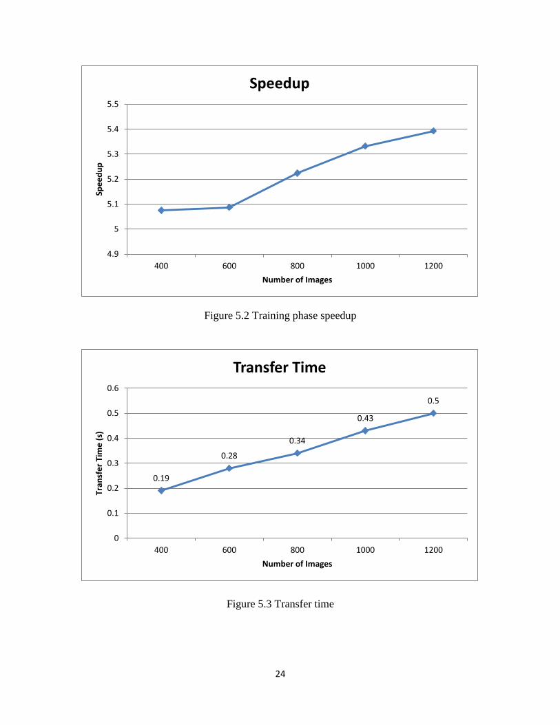
The total execution time of training phase, which includes normalization, covariance, jacobi,
eigenface and weights module, is shown in table 5.8 and speedup is shown in figure 5.2. Training
phase has shown overall speedup of 5x.
Time required for transferring training images data from CPU to GPU is shown in fig 5.3. As
compared to computation time, the transfer time is very low.
Table 5.8 Execution Time and speedup of training phase
No of Images Serial Time (In seconds) Parallel Time ( In seconds) Speedup
400 434.34 85.58 5.07x
600 1878.38 369.29 5.09x
800 5540.00 1060.53 5.22x
1000 13343.20 2502.60 5.33x
1200 27087.00 5022.92 5.40x
0
20
40
60
80
100
120
140
160
400 600 800 1000 1200
Spe
ed
up
Number of Images
Normalization
Covariance
Jaconbi
Eigenface
Weights
Recognition
24
Figure 5.2 Training phase speedup
Figure 5.3 Transfer time
4.9
5
5.1
5.2
5.3
5.4
5.5
400 600 800 1000 1200
Spe
ed
up
Number of Images
Speedup
0.19
0.28
0.34
0.43
0.5
0
0.1
0.2
0.3
0.4
0.5
0.6
400 600 800 1000 1200
Tran
sfe
r Ti
me
(s)
Number of Images
Transfer Time

25
Chapter 6
Conclusion and Future Work
6.1 Conclusion
Eigenface algorithm consists of various data parallelism tasks which require high computation
mainly in the training phase. The parallel CUDA implementation of eigenface algorithm has
shown an overall speedup of 5x in the training phase. The speedup increases with the increase in
training database. In training phase, eigenface computation module has shown highest speedup
of 148x. The Jacobi module has shown the lowest performance gain among the entire training
phase modules with the speedup of 3x to 5x. Recognition phase has shown little speedup, which
increases with increase in the training database. Recognition phase is faster on CPU for small
database, but it requires copying data from GPU to CPU which takes some time. To avoid
copying, the recognition module is best kept on GPU.
6.2 Future Work
Future work will include implementing Jacobi module using dynamic parallelism. The Jacobi
module requires launching a CUDA kernel at each CPU iteration and a memory copy from
device to host at every 10000 iteration to check for convergence. Kernel launch from host and
memory copy from device to host is a time consuming process. Dynamic parallelism supports
launching a CUDA kernel from a CUDA kernel, which is faster than launching a kernel from
CPU. With dynamic parallelism, in Jacobi module, only one kernel has to be launched from host
and the memory copy will also not require. Dynamic parallelism is available on NVidia GPUs
having compute capability 3.5 or higher. With the advancements in GPUs, it is possible to get
much higher performance gain.

26
Bibliography
[1]. Matthew A. Turk, Alex P. Pentland, “Face Recognition Using Eigenfaces”, Proc IEEE
Conferene on Computer Vision and Pattern Recognition, 1991.
[2]. L. Sirovich and M. Kirby, “Low-dimensional Procedure for the characterization of
human faces”, Journal of the Optical Society of America A4(3): 519-524.
[3]. Karl Pearson (1901), “On Lines and Planes of Closest Fit to Systems of Points in Space”,
Philosophical Magazine 2(11): 559/572.
[4]. Prof. V.P. Kshirsagar, M.R.Baviskar, M.E.Gaikwad, “Face Recognition Using
Eigenfaces”, Intennational conference on Computer research and development 2011.
[5]. Wendy S., Yambor, Bruce A. Draper and J. Ross Beveridge, “Analyzing PCA-based
Face Recognition Algorithms: Eigenvector Selection and Distance Measures”, Second
Workshop on Empirical Evaluation in Computer Vision, 39-60, 2000.
[6]. Christopher Mallow, “Authentication Methods and Techniques”, CISSP
[7]. Patrik Kamencay, Martin Breznan, Dominik Jelsovka, Martina Zacharisova, “Improved
Face Recognition method based on Segmentation Algorithm using SIFT-PCA”, TSP,
page 758-762. IEEE, (2012)
[8]. Wlodzimierz M. Baranski, Andrzej Wytyczak-Partyka, Tomasz Walkowiak,
“Computational complexity reduction in PCA-based face recognition”, Institute of
Computer Engineering, Control and Robotics, Wroclaw University of Technology,
Poland.
[9]. Neeraja, Ekta Walia, “Face Recognition Using Improved Fast PCA Algorithm”,
Congress on Image and Signal Processing.
[10]. Tao Wang, Longjiang Guo , Guilin Li , Jinbao L , Renda Wang, Meirui Ren,
“Implementing the Jacobi Algorithm for solving Eigenvalues of Symmetric Matrices
with CUDA”, IEEE Seventh International Conference on Networking, Architecture and
storage, 2012.
[11]. D. B. Kirk and W. mei W. Hwu, “Programming Massively Parallel Processors: A
Hands-on Approach”, Morgan Kaufmann, 2010.
[12]. Hennessy, John L., David A., Patterson, “Computer Architecture: A Quantitive
Approach”, Morgan Kaufmann, 46-47, 2012

27
[13]. P. J. Phillips, H. Wechsler, J. Huang, P.Rauss, “The FERET database and evaluation
procedure for face recognition algorithms”, Image and Vision Computing J, Vol. 16, No.
5, 295-306, 1998.
[14]. Jason Sanders, Edward Kandrot, “CUDA by Example: An Introduction to general-
Purpose GPU Programming”, Addison-Welsey.