Parallel Data Processing†

Introduction to DatabasesCompSci 316 Fall 2019

†Some contents are drawn and adapted from slides by Madga Balazinska at U. Washington

Announcements (Wed., Nov. 20)

• Homework 4 due Mon. after Thanksgiving break• Piazza project weekly progress update due today

2

Announcements (Mon., Nov. 25)

• Homework 4 due in a week• No Piazza project weekly update due this week

3

Parallel processing

• Improve performance by executing multiple operations in parallel• Cheaper to scale than relying on a single

increasingly more powerful processor• Performance metrics• Speedup, in terms of completion time• Scaleup, in terms of time per unit problem size• Cost: completion time × # processors × (cost per

processor per unit time)

4

Speedup

• Increase # processors → how much faster can we solve the same problem?• Overall problem size is fixed

5

# processors

spee

dup

1

1×

linear s

peedup (ideal) reality

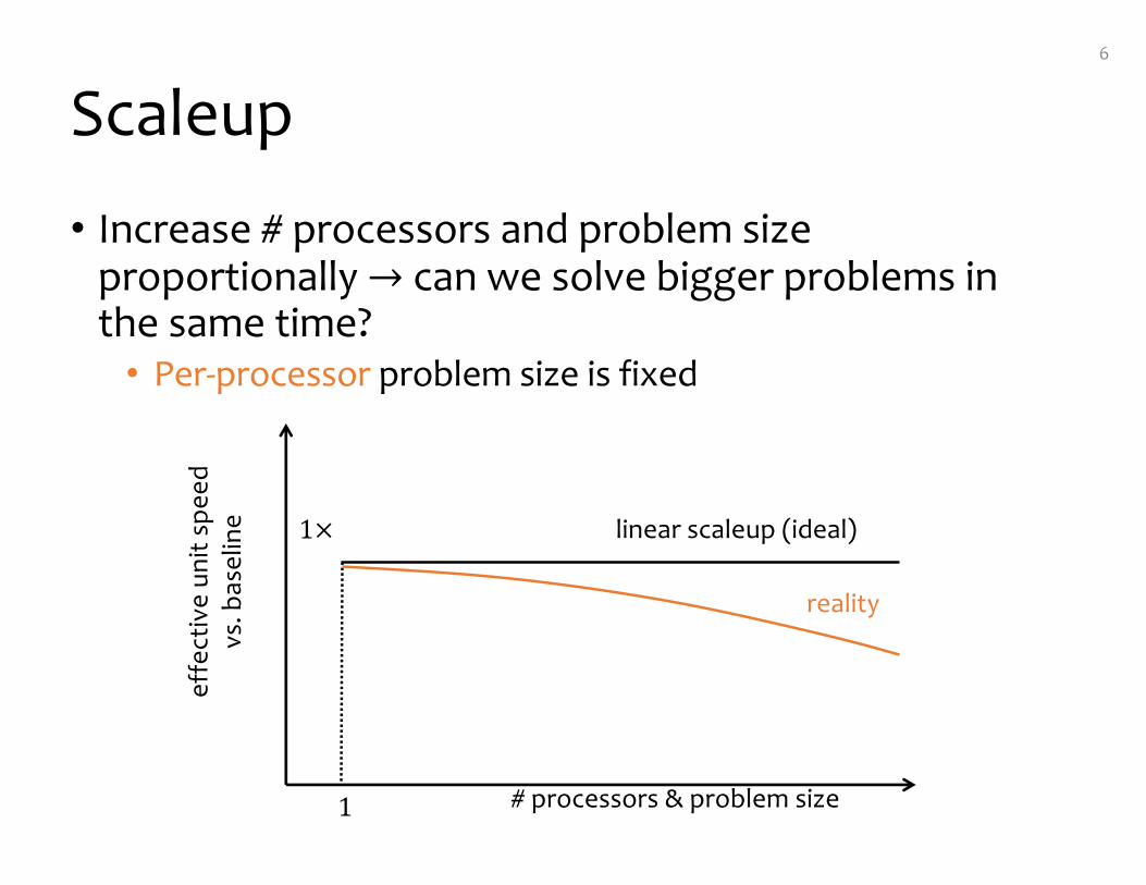
Scaleup

• Increase # processors and problem size proportionally → can we solve bigger problems in the same time?• Per-processor problem size is fixed

6

# processors & problem size

effe

ctiv

e un

it sp

eed

vs. b

asel

ine

1

1× linear scaleup (ideal)

reality

Cost

• Fix problem size

• Increase problem size proportionally with # processors

7

# processors

cost

1

1×linear speedup (ideal)

reality

# processors & problem size

cost

per

unit

prob

lem

siz

e

1

1×linear scaleup (ideal)

reality

Why linear speedup/scaleup is hard

• Startup• Overhead of starting useful work on many processors

• Communication• Cost of exchanging data/information among processors

• Interference• Contention for resources among processors

• Skew• Slowest processor becomes the bottleneck

8

Shared-nothing architecture

• Most scalable (vs. shared-memory and shared-disk)• Minimizes interference by minimizing resource sharing• Can use commodity hardware

• Also most difficult to program

9

Disk Disk Disk

Mem Mem Mem

Proc Proc Proc

Interconnection network

Parallel query evaluation opportunities

• Inter-query parallelism• Each query can run on a different processor

• Inter-operator parallelism• A query runs on multiple processors• Each operator can run on a different processor

• Intra-operator parallelism• An operator can run on multiple processors, each

working on a different “split” of data/operation☞Focus of this lecture

10

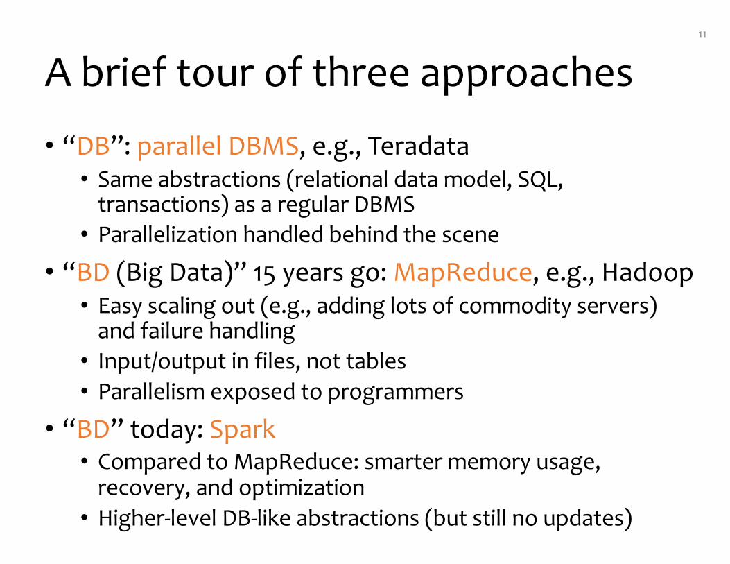
A brief tour of three approaches

• “DB”: parallel DBMS, e.g., Teradata• Same abstractions (relational data model, SQL,

transactions) as a regular DBMS• Parallelization handled behind the scene

• “BD (Big Data)” 15 years go: MapReduce, e.g., Hadoop• Easy scaling out (e.g., adding lots of commodity servers)

and failure handling• Input/output in files, not tables• Parallelism exposed to programmers

• “BD” today: Spark• Compared to MapReduce: smarter memory usage,

recovery, and optimization• Higher-level DB-like abstractions (but still no updates)

11

Parallel DBMS

12

E.g.:

Horizontal data partitioning

• Split a table ! into " chunks, each stored at one of the " processors• Splitting strategies:• Round robin assigns the #-th row assigned to chunk # mod "

• Hash-based partitioning on attribute ' assigns row ( to chunk ℎ (. ' mod "• Range-based partitioning on attribute ' partitioning the

range of !. ' values into " ranges, and assigns row ( to the chunk whose corresponding range contains (. '

13

Teradata: an example parallel DBMS

• Hash-based partitioning of Customer on cid

14

A Customer row is inserted

AMP 1

AMP 2

AMP 3

AMP 4

AMP 5

AMP 6

AMP 7

AMP 8

AMP …

AMP …

AMP …

AMP …

AMP …

AMP …

AMP …

AMP …

…

hash(cid)

AMP = unit of parallelism in TeradataNode 1 Node 2

Each Customer is assigned to an AMP

Example query in Teradata

• Find all orders today, along with the customer info

SELECT *FROM Order o, Customer cWHERE o.cid = c.cidAND o.date = today();

15

join

scanfilter

scan

o.cid = c.cid

o.date = today()

Order oCustomer c

Teradata example: scan-filter-hash16

join

scanfilter

scan

o.cid = c.cid

o.date = today()

Order oCustomer c

hash

filter

scan

o.cid

o.date = today()

Order o

AMP AMP AMP

AMP AMP AMPConsistent with partitioning of Customer; each Order row is routed to the AMP storing the Customerrow with the same cid

hash

filter

scan

o.cid

o.date = today()

Order o

hash

filter

scan

o.cid

o.date = today()

Order o

Teradata example: hash join17

AMP

join

scan

o.cid = c.cid

Customer c

Each AMP processes Order and Customerrows with the same cid hash

join

scanfilter

scan

o.cid = c.cid

o.date = today()

Order oCustomer c

AMP

join

scan

o.cid = c.cid

Customer cAMP

join

scan

o.cid = c.cid

Customer c

18

MapReduce: motivation

• Many problems can be processed in this pattern:• Given a lot of unsorted data• Map: extract something of interest from each record• Shuffle: group the intermediate results in some way• Reduce: further process (e.g., aggregate, summarize,

analyze, transform) each group and write final results(Customize map and reduce for problem at hand)

FMake this pattern easy to program and efficient to run• Original Google paper in OSDI 2004• Hadoop has been the most popular open-source

implementation• Spark still supports it

19

M/R programming model

• Input/output: each a collection of key/value pairs• Programmer specifies two functions• map $%, '% → list $-, '-

• Processes each input key/value pair, and produces a list of intermediate key/value pairs

• reduce $-, list '- → list '3• Processes all intermediate values associated with the same key,

and produces a list of result values (usually just one for the key)

20

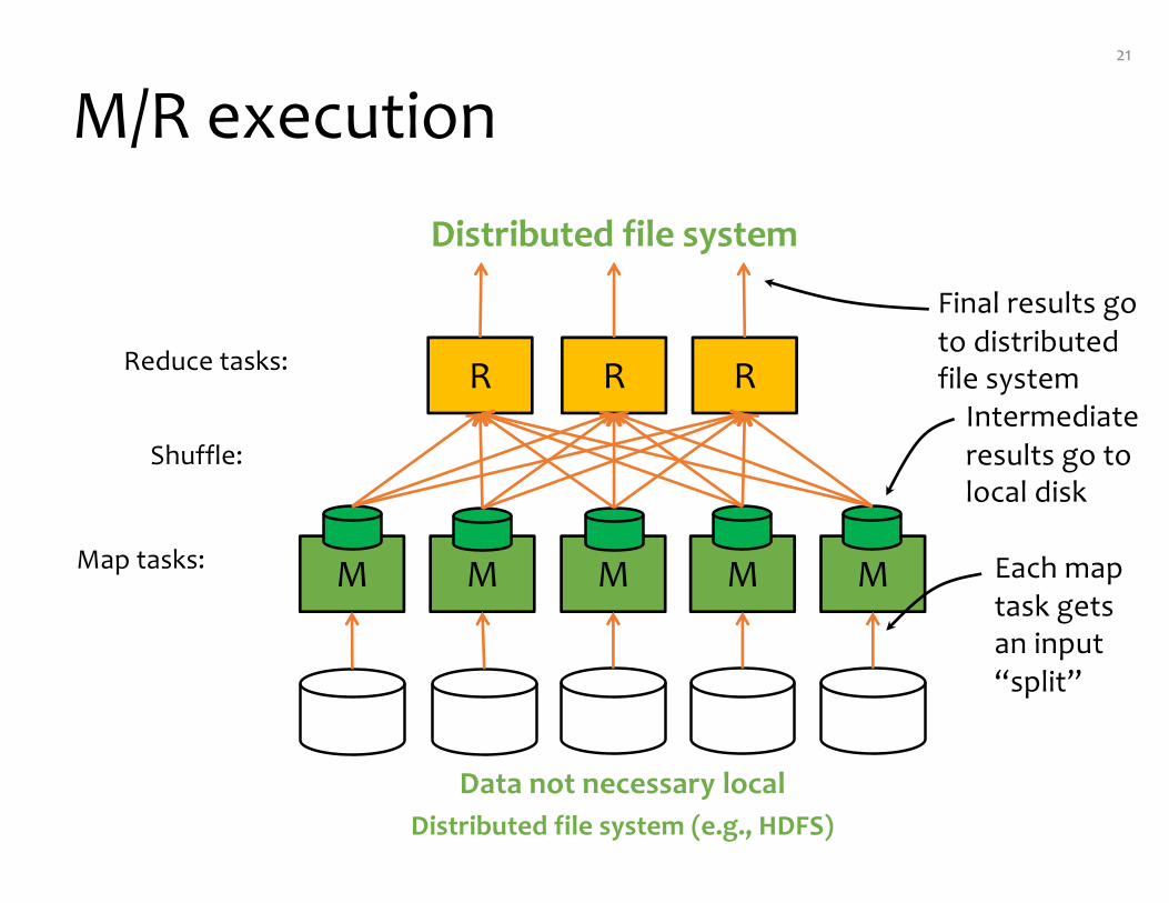
M/R execution21

Data not necessary localDistributed file system (e.g., HDFS)

M M M M M

R R R

Distributed file system

Final results go to distributedfile systemReduce tasks:

Map tasks:

Shuffle:

Each map task gets an input “split”

Intermediate results go to local disk

M/R example: word count• Expected input: a huge file (or collection of many

files) with millions of lines of English text• Expected output: list of (word, count) pairs• Implementation• map _, line → list word, count

• Given a line, split it into words, and output 3, 1 for each word 3 in the line

• reduce word, list count → word, count• Given a word 3 and list 5 of counts associated with it, compute 6 = ∑9:;<=∈? count and output 3, 6

• Optimization: before shuffling, map can pre-aggregate word counts locally so there is less data to be shuffled• This optimization can be implemented in Hadoop as a

“combiner”

22

Some implementation details

• There is one “master” node• Input file gets divided into ! “splits,” each a

contiguous piece of the file• Master assigns ! map tasks (one per split) to

“workers” and tracks their progress• Map output is partitioned into " “regions”• Master assigns " reduce tasks (one per region) to

workers and tracks their progress• Reduce workers read regions from the map

workers’ local disks

23

M/R execution timeline

• When there are more tasks than workers, tasks execute in “waves”• Boundaries between waves are usually blurred

• Reduce tasks can’t start until all map tasks are done

24

M

M

M M

M

M

R

R

R

R

R

RM M

M M

time

More implementation details

• Numbers of map and reduce tasks• Larger is better for load balancing• But more tasks add overhead and communication

• Worker failure• Master pings workers periodically• If one is down, reassign its split/region to another

worker

• “Straggler”: a machine that is exceptionally slow• Pre-emptively run the last few remaining tasks

redundantly as backup

25

M/R example: Hadoop TeraSort

• Expected input: a collection of (key, payload) pairs

• Expected output: sorted (key, payload) pairs

• Implementation• Using a small sample of input, find ! − 1 key values that

divides the key range into ! subranges where # pairs is roughly equal across them

• map ', payload → ., ', payload• If ' falls within the .-th subrange

• reduce ., list ', payload → list ', payload• Sort the list of ', payload pairs by ' and output

26

Parallel DBMS vs. MapReduce

• Parallel DBMS• Schema + intelligent indexing/partitioning• Can stream data from one operator to the next• SQL + automatic optimization

• MapReduce• No schema, no indexing• Higher scalability and elasticity

• Just throw new machines in!

• Better handling of failures and stragglers• Black-box map/reduce functions → hand optimization

27

28

We will focus on the Python dialect, although Spark supports multiple languages

Addressing inefficiencies in Hadoop

• Hadoop: no automatic optimization

☞Spark

• Allow program to be a DAG of DB-like operators, with

less reliance on black-box code

• Delay evaluation as much as possible

• Fuse operators into stages and compile each stage

• Hadoop: too many I/Os

• E.g., output of each M/R job is always written to disk

• But such checkpointing simplifies failure recovery

☞Spark

• Keep intermediate results in memory

• Instead of checkpointing, use “lineage” for recovery

29

RDDs

• Spark stores all intermediate results as Resilient Distributed Datasets (RDDs)• Immutable, memory-resident, and distributed across

multiple nodes

• Spark also tracks the “lineage” of RDDs, i.e., what expressions computed them• Can be done at the partition level

What happens to a RDD if a node crashes?• The partition of this RDD on this node will be lost• But with lineage, the master simply recomputes the

a lost partition when needed• Requires recursive recomputation if input RDD partitions

are also missing

30

Example: votes & explanations

• Raw data reside in lots of JSON files obtained from

ProPublica API

• Each vote: URI (id), question, description, date,

time, result

• Each explanation: member id, name, state, party,

vote URI, date, text, category

• E.g., “P000523”, “David E. Price”, “NC”, “D”,

“https://api.propublica.org/congress/v1/115/house/sessio

ns/2/votes/269.json”, “2018-06-20”, “Mr. Speaker, due to

adverse weather and numerous flight delays and

cancellations in North Carolina, I was unable to vote

yesterday during Roll Call 269, the motion…”, “Travel

difficulties”

31

Basic M/R with Spark RDDexplain_fields = ('member_id', 'name', 'state', 'party', 'vote_api_uri’,

'date', 'text', 'category')

# Map function:

def map(record):

if len(record) == len(explain_fields):

return [(record[explain_fields.index('category')], 1)]

else:

return []

# Reduce function:

def reduce(record):

key, vals = record

return [(key, len(vals))]

32

map $%, '% → list $-, '-

reduce $-, list '- → list '3

Basic M/R with Spark RDD# setting up one RDD that contains all the input:

rdd = sc. ...

# count number of explanations by category; order by

# number (descending) and then category (ascending):

result = rdd\

.flatMap(map)\

.groupByKey()\

.flatMap(reduce)\

.sortBy(lambda x: (-x[1], x[0]))

for row in result.collect():

print('|'.join(str(field) for field in row))

33

Be lazy: build up a DAG of “transformations,” but no evaluation yet!

Optimize & evaluate the whole DAG only when needed, e.g., triggered by “actions” like collect()

Be careful: Spark RDDs support map() and reduce() too, but they are not the same as those in MapReduce

Moving “BD” to “DB”

Each element in a RDD is an opaque object—hard to program

• Why don’t we make each element a “row” with named columns—easier to refer to in processing• RDD becomes a DataFrame (name from the R language)

• Still immutable, memory-resident, and distributed

• Then why don’t we have database-like operators instead of just MapReduce?• Knowing their semantics allows more optimization

• Spark in fact pushed the idea further• Spark Dataset = DataFrame with type-checking

• And just run SQL over Datasets using SparkSQL!

34

Spark DataFramefrom pyspark.sql import functions as F

explain_fields = ('member_id', 'name', 'state', 'party', 'vote_api_uri’,'date', 'text', 'category’)

# setting up a DataFrame of explanations:

df_explain = sc. ...

# count number of explanations by category; order by

# number (descending) and then category (ascending):

df_explain.groupBy('category')\

.agg(F.count('name'))\

.withColumnRenamed('count(name)', 'count')\

.sort(['count', 'category'], ascending=[0, 1])\

.show(20, truncate=False)

35

Another Spark DataFrame Example36

from pyspark.sql import functions as F

vote_fields = ('vote_uri','question','description','date','time','result')

explain_fields = ('member_id', 'name', 'state', 'party', 'vote_api_uri’,'date', 'text', 'category’)

# setting up DataFrames for each type of data:

df_votes = sc. ...

df_explain = sc. ...

# what does the following do?

df_votes.join(df_explain.select('vote_api_uri', 'name'),

df_votes.vote_uri == df_explain.vote_api_uri, 'left_outer')\

.groupBy('vote_uri', 'date', 'time', 'question', 'description', 'result')\

.agg(F.count('name'), F.collect_list('name'))\

.withColumnRenamed('count(name)', 'count')\

.withColumnRenamed('collect_list(name)', 'names')\

.sort(['count', 'date', 'time'], ascending=[0, 0, 0])\

.select('vote_uri', 'date', 'time', 'question', 'description', 'result’,

'count', 'names’)\

.show(20, truncate=False)

For each vote, find out which legislators provided explanations; order by the number of such legislators (descending), then date and time (descending)

Summary

• “DB”: parallel DBMS• Standard relational operators• Automatic optimization• Transactions

• “BD” 15 years go: MapReduce• User-defined map and reduce functions• Mostly manual optimization• No updates/transactions

• “BD” today: Spark• Still supporting user-defined functions, but more

standard relational operators than older “BD” systems• More automatic optimization than older “BD” systems• No updates/transactions

37