parallel and distributed successive convex … · 2 gesualdo scutari and ying sun introduction...
TRANSCRIPT
Parallel and Distributed Successive ConvexApproximation Methods for Big-DataOptimization
Gesualdo Scutari and Ying Sun
January 15, 2018
Lecture Notes in Mathematics, C.I.M.E, Springer Verlag series
Gesualdo ScutariPurdue University, West Lafayette, IN, USA, e-mail: [email protected]
Ying SunPurdue University, West Lafayette, IN, USA, e-mail: [email protected]
This work has been partially supported by the USA National Science Foundation under GrantsCIF 1564044, CIF 1719205, and CAREER Award 1555850; and in part by the Office of NavalResearch under Grant N00014-16-1-2244.
1
2 Gesualdo Scutari and Ying Sun
Introduction
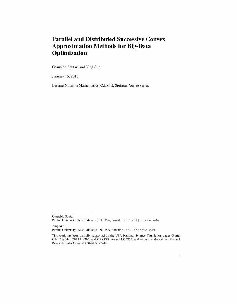
Recent years have witnessed a surge of interest in parallel and distributed optimiza-tion methods for large-scale systems. In particular, nonconvex large-scale optimiza-tion problems have found a wide range of applications in several engineering fieldsas diverse as (networked) information processing (e.g., parameter estimation, detec-tion, localization, graph signal processing), communication networks (e.g., resourceallocation in peer-to-peer/multi-cellular systems), sensor networks, data-based net-works (including Facebook, Google, Twitter, and YouTube), swarm robotic, andmachine learning (e.g., nonlinear least squares, dictionary learning, matrix comple-tion, tensor factorization), just to name a few–see Figure 1.
The design and the analysis of such complex, large-scale, systems pose severalchallenges and call for the development of new optimization models and algorithms.
- Big-Data: Many of the aforementioned applications lead to huge-scale optimiza-tion problems (i.e., problems with a very large number of variables). Theseproblems are often referred to as big-data. This calls for the developmentof solution methods that operate in parallel, exploiting hierarchical compu-tational architectures (e.g., multicore systems, cluster computers, cloud-basednetworks), if available, to cope with the curse of dimensionality and accommo-date the need of fast (real-time) processing and optimization. The challenge isthat such optimization problems are in general not separable in the optimizationvariables, which makes the design of parallel schemes not a trivial task.
- In-network optimization: The networked systems under consideration are typ-ically spatially distributed over a large area (or virtually distributed). Due to
Distributed Nonconvex Decision/Learning
Fig. 1: A bird’s-eye view of some relevant applications generating nonconvex large-scale (net-worked) optimization problems.
Title Suppressed Due to Excessive Length 3
the size of such networks (hundreds to millions of agents), and often to theproprietary regulations, these systems do not possess a single central coordina-tor or access point with the complete system information, which is thus ableto solve alone the entire optimization problem. Network/data information is in-stead distributed among the entities comprising the network. Furthermore, thereare some networks such as surveillance networks or some cyber-physical sys-tems, where a centralized architecture is not desirable, as it makes the systemprone to central entity fails and external attacks. Additional challenges are en-countered from the network topology and connectivity that can be time-varying,due, e.g., to link failures, power outage, and agents’ mobility. In this setting,the goal is to develop distributed solution methods that operate seamless in-network, by leveraging the network connectivity and local information (e.g.,neighbor information) to cope with the lack of global knowledge on the op-timization problem and offer robustness to possible failures/attacks of centralunits and/or to time-varying connectivity.
- Nonconvexity: Many formulations of interest are nonconvex, with nonconvex ob-jective functions and/or constraints. Except for very special classes of noncon-vex problems, whose solution can be obtained in closed form, computing theglobal optimal solution might be computationally prohibitive in several practi-cal applications. This is the case, for instance, of distributed systems composedof workers with limited computational capabilities and power (e.g., motes orsmart dust sensors). The desiderata is designing (parallel/distributed) solutionmethods that are easy to implement (in the sense that the computations per-formed by the workers are not expensive), with provable convergence to station-ary solutions of the nonconvex problem under consideration (e.g., local optimalsolutions). To this regard, a powerful and general tool is offered by the so-calledSuccessive Convex Approximation (SCA) techniques: as proxy of the noncon-vex problem, a sequence of “more tractable” (possibly convex) subproblemsis solved, wherein the original nonconvex functions are replaced by properlychosen “simpler” surrogates. By tailoring the choice of the surrogate functionsto the specific structure of the optimization problem under consideration, SCAtechniques offer a lot of freedom and flexibility in the algorithmic design.
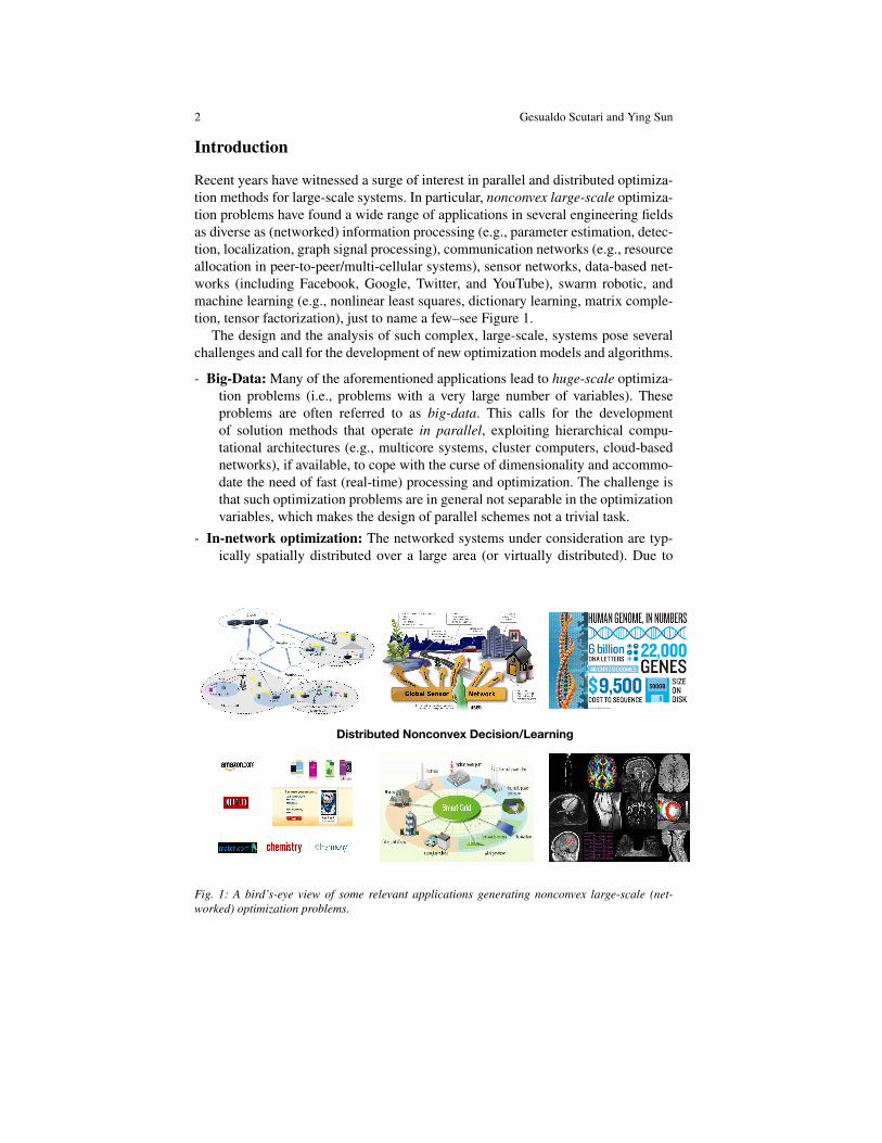
As a concrete example, consider the emerging field of in-network big-data an-alytics: the goal is to preform some, generally nonconvex, analytic tasks from asheer volume of data, distributed over a network–see Fig. 2–examples include ma-chine learning problems such as nonlinear least squares, dictionary learning, ma-trix completion, and tensor factorization, just to name a few. In these data-intensiveapplications, the huge volume and spatial/temporal disparity of data render central-ized processing and storage a formidable task. This happens, for instance, wheneverthe volume of data overwhelms the storage capacity of a single computing device.Moreover, collecting sensor-network data, which are observed across a large numberof spatially scattered centers/servers/agents, and routing all this local information tocentralized processors, under energy, privacy constraints and/or link/hardware fail-ures, is often infeasible or inefficient.
4 Gesualdo Scutari and Ying Sun
In-network Processing
Processing Explosion
TrafficExplosion
Centralized Processing
Fig. 2: In-network big-data analytics: Traditional centralized processing and optimization are of-ten infeasible or inefficient when dealing with large volumes of data distributed over large-scalenetworks. There is a necessity to develop fully decentralized algorithms that operate seamless in-network.
The above challenges make the traditional (centralized) optimization and con-trol techniques inapplicable, thus calling for the development of new computationalmodels and algorithms that support efficient, parallel and distributed nonconvex op-timization over networks. The major contribution of this paper is to put forth a gen-eral, unified, algorithmic framework, based on SCA techniques, for the parallel anddistributed solution of a general class of non-convex constrained (non-separable)problems. The presented framework unifies and generalizes several existing SCAmethods, making them appealing for a parallel/distributed implementation while of-fering a flexible selection of function approximants, step size schedules, and controlof the computation/communication efficiency.
This paper is organized according to the lectures that one of the authors deliveredat the CIME Summer School on Centralized and Distributed Multi-agent Optimiza-tion Models and Algorithms held in Cetraro, Italy, June 23–27, 2014. These lecturesare:Lecture I–Successive Convex Approximation Methods: Basics.Lecture II–Parallel Successive Convex Approximation Methods.Lecture III–Distributed Successive Convex Approximation Methods.Omissions: Consistent with the main theme of the Summer School, the lecturesaim at presenting SCA-based algorithms as a powerful framework for parallel anddistributed, nonconvex multi-agent optimization. Of course, other algorithms havebeen proposed in the literature for parallel and distributed optimization. This paperdoes not cover schemes that are not directly related to SCA-methods or provablyapplicable to nonconvex problems. Examples of omissions are: primal-dual meth-ods; augmented Lagrangian methods, including the alternating direction methods ofmultipliers (ADMM); and Newton methods and their inexact versions. When rele-vant, we provide citations of the omitted algorithms at the end of each lecture, in thesection of “Source and Notes”.

Title Suppressed Due to Excessive Length 5
Lecture I – Successive Convex Approximation Methods: Basics
This lecture overviews the majorization-minimization (MM) algorithmic frame-work, a particular instance of Successive Convex Approximation (SCA) Methods.The MM basic principle is introduced along with its convergence properties, whichwill set the ground for the design and analysis of SCA-based algorithms in the sub-sequent lectures. Several examples and applications are also discussed.
Consider the following general class of nonconvex optimization problems
minimizex∈X
V (x), (1)
where X ⊆Rm is a nonempty closed convex set and V : O→R is continuous (possi-bly nonconvex and nonsmooth) on O, an open set containing X . Further assumptionson V are introduced as needed.
The MM method applied to Problem (1) is based on the solution of a sequenceof “more tractable” subproblems whereby the objective function V is replaced by a“simpler” suitably chosen surrogate function. At each iteration k, a subproblem issolved of the type
xk+1 ∈ argminx∈X
V (x |xk), (2)
where V (•|xk) is a surrogate function (generally dependent on the current iterate xk)that upperbounds V globally (further assumptions on V are introduced as needed).The sequence of majorization-minimization steps are pictorially shown in Fig. I.1.The underlying idea of the approach is that the surrogate function V is chosen so thatthe resulting subpoblem (2) can be efficiently solved. Roughly speaking, surrogatefunctions enjoying the following features are desirable:
• (Strongly) Convexity: this would lead to (strongly) convex subproblems (2);• (Additively) Block-separability in the optimization variables: this is a key en-
abler for parallel/distributed solution methods, which are desirable to solvelarge-scale problems;• Minimizer over X in closed-form: this reduces the cost per iteration of the MM
algorithm.
Finding the “right” surrogate function for the problem under consideration (pos-sibly enjoying the properties above) might not be an easy task. A major goal ofthis section is to put forth general construction techniques for V and show their ap-plication to some representative problems in signal processing, data analysis, andcommunications. Some instances of V are drawn from the literature, e.g., [228],while some others are new and introduced for the first time in this chapter. Therest of this lecture is organized as follows. After introducing in Sec. I.1 some basicresults which will lay the foundations for the analysis of SCA methods in the sub-sequent sections, in Sec. I.2 we describe in details the MM framework along withits convergence properties; several examples of valid surrogate functions are alsodiscussed (cf. Sec. I.2.1). When the surrogate function V is block separable and so

6 Gesualdo Scutari and Ying Sun
xkxk xk+1xk+1 xk+2xk+2
V (x)V (x)
eV (x j xk)eV (x j xk)
eV (x j xk+1)eV (x j xk+1)
V (xk+1) · V (xk)V (xk+1) · V (xk)
Fig. I.1: Pictorial description of the MM procedure.
are the constraints in (2), subproblems (2) can be solved leveraging parallel algo-rithms. For unstructured functions V , in general separable surrogates are difficult tobe found. When dealing with large scale optimization problems, solving (2) with re-spect to all variables might not be efficient or even possible; in all these cases, paral-lel block schemes are mandatory. This motivates the study of so-called “block MM”algorithms only some blocks of the variables are selected and optimized at a time.Sec. I.3 is devoted to the study of such algorithms. In Sec. I.4 we will present severalapplications of MM methods to problems in signal processing, machine learning,and communications. Finally, in Sec. I.5 we overview the main literature and high-light some extensions and generalizations of the methods described in this lecture.
I.1. Preliminaries
We introduce here some preliminary basic results which will be extensively usedthrough the whole paper.
We begin with the definition of directional derivative of a function and somebasic properties of directional derivatives.
Definition I.1 (directional derivative). A function f : Rm → (−∞,∞] is direction-ally differentiable at x ∈ dom f , x ∈ Rm : f (x)< ∞ along a direction d ∈ Rm ifthe following limit
f ′ (x;d), limλ↓0
f (x+λd)− f (x)λ
(3)
exists; this limit f ′ (x;d) is called the directional derivative of f at x along d. If f isdirectionally differentiable at x along all directions, then we say that f is direction-ally differentiable at x.

Title Suppressed Due to Excessive Length 7
If f is differentiable at x, then f ′ (x;d) reads: f ′ (x;d) = ∇ f (x)T d, where ∇ f (x)is the gradient of f at x. Some examples of directional derivatives of some structuredfunctions (including convex functions) are discussed next.• Case study 1: Convex functions. Throughout this example, we assume thatf : Rm → (−∞,∞] is a convex, closed, proper function; and int(dom f ) 6= /0 (oth-erwise, one can work with the relative interior of dom f ), with int(dom f ) denotingthe interior of dom f .
We show next that if x ∈ dom f , f ′ (x;d) is well defined, taking values in[−∞,+∞]. In particular, if x ∈ dom f can be approached by the direction d ∈ Rm,then f ′ (x;d) is finite. For x ∈ dom f , d ∈ Rm and nonzero λ ∈ R, define
λ 7→ gλ (x;d),f (x+λd)− f (x)
λ.
A simple argument by convexity (increasing slopes) shows that g(d;λ ) is increasingin λ . Therefore, the limit in (3) exists in [−∞,∞] and can be replaced by
f ′ (x;d) = infλ>0
1λ[ f (x+λd)− f (x)] .
Moreover, for 0 < λ ≤ β ∈ R, it holds
g−β (x;d)≤ g−λ (x;d)≤ gλ (x;d)≤ gβ (x;d).
If x∈ int(dom f ), both g−β (x;d) and gβ (x;d) are finite, for sufficiently small β > 0;therefore, we have
−∞ < g−β (x;d)≤ f ′ (x;d) = infλ>0
gλ (d;x)≤ gβ (x;d)<+∞.
Finally, since f is convex, it is locally Lipschitz continuous: for sufficiently smallβ > 0, there exists some finite L > 0 such that gβ (x;d) ≤ L‖d‖ and g−β (x;d) ≥−L‖d‖. We have proved the following result.
Proposition I.2. For convex functions f : Rm→ (−∞,∞], at any x ∈ dom f and forany d ∈Rm, the directional derivative f ′ (x;d) exists in [−∞,+∞] and it is given by
f ′ (x;d) = infλ>0
1λ[ f (x+λd)− f (x)] .
If x∈ int(dom f ), there exists a finite constant L > 0 such that | f ′ (x;d) | ≤ L‖d‖, forall d ∈ Rm.
Directional derivative and subgradients. The directional derivative of a convexfunction can be also written in terms of its subgradients, as outlined next. We firstintroduce the definition of subgradient along with some of its properties.
Definition I.3 (subgradient). A vector ξξξ ∈ Rm is a subgradient of f at a point x ∈dom f if
8 Gesualdo Scutari and Ying Sun
f (x+d)≥ f (x)+ξξξT d, ∀d ∈ Rm. (4)
The subgradient set (a.k.a. subdifferential) of f at x ∈ dom f is defined as
∂ f (x),
ξξξ ∈ Rm : f (x+d)≥ f (x)+ξξξT d, ∀d ∈ Rm . (5)
Partitioning x in blocks, x = (xi)ni=1, with xi ∈Rmi and ∑
ni=1 mi = m, similarly to
(5), we can define the block-subdifferential with respect to each xi, as given below,where (x)i , (0T , . . . ,xT
i , . . . ,0T )T ∈ Rm.
Definition I.4 (block-subgradient). The subgradient set ∂i f (x) of f at x=(xi)ni=1 ∈
dom f with respect to xi is defined as
∂i f (x),
ξξξ i ∈ Rmi : f (x+(d)i)≥ f (x)+ξξξTi di, ∀di ∈ Rmi
. (6)
Intuitively, when a function f is convex, the subgradient generalizes the deriva-tive of f ; in fact, f (x) +ξξξ T d is a global linear underestimator of f at x. Sincea convex function has global linear underestimators of itself, the subgradient set∂ f (x) should be non-empty and consist of supporting hyperplanes to the epigraphof f . This is formally stated in the next result (see, e.g., [24, 102] for the proof).
Theorem I.5. Let x ∈ int(dom f ). Then, ∂ f (x) is nonempty, compact, and convex.
Note that, in the above theorem, we cannot relax the assumption x∈ int(dom f ) withx∈ dom f . For instance, consider the function f (x) =−√x, with dom f = [0,∞). Wehave ∂ f (0) = /0.
The subgradient definition describes a global properties of the function whereasthe (directional) derivative is a local property. The connection between a directionalderivative and the subdifferential of a convex function is contained in the next tworesults, whose proof can be found in [24, Ch.3].
Lemma I.6. The subgradient set (5) at x ∈ dom f can be equivalently written as
∂ f (x),
ξξξ ∈ Rm : f ′(x;d)≥ ξξξT d, ∀d ∈ Rm . (7)
Note that, since f ′(x;d) is finite for all d ∈ Rm (cf. Proposition I.2), the aboverepresentation readily shows that ∂ f (x), x ∈ int(dom f ), is a compact set (as provedalready in Theorem I.5). Furthermore, ξξξ ∈ ∂ f (x) satisfies
‖ξξξ‖2 = supd :‖d‖2≤1
ξξξT d≤ sup
d :‖d‖2≤1f ′(x;d)< ∞.
Lemma I.6 above showed how to identify subgradients from directional deriva-tive. Lemma I.7 below shows how to move in the reverse direction.
Lemma I.7 (max formula). At any x ∈ int(dom f ) and all d ∈ Rm, it holds
f ′(x;d) = supξξξ∈∂ f (x)
ξξξT d. (8)

Title Suppressed Due to Excessive Length 9
Lastly, we recall a straightforward result, stating that the subgradient is simply thegradient of differentiable convex functions. This is a direct consequence of LemmaI.6. Indeed, if f is differentiable at x, we can write [cf. (7)]
ξξξT d≤ f ′(x;d) = ∇ f (x)T d, ∀ξξξ ∈ ∂ f (x).
Since the above inequality holds for all d∈Rm, we also have ξξξ T (−d)≤ f ′(x;−d)=∇ f (x)T (−d), and thus ξξξ T d = ∇ f (x)T d, for all d ∈ Rm. This proves ∂ f (x) =∇ f (x).
The subgradient is also intimately related to optimality conditions for convexminimization. We discuss this relationship in the next subsection. We conclude thisbrief review with some basic examples of calculus of subgradient.Examples of subgradients. As the first example, consider
f (x) = |x|.
It is not difficult to check that
∂ |x|=
sign(x), if x 6= 0;[−1, 1] if x = 0;
(9)
where sign(x) = 1, if x > 0; sign(x) = 0, if x = 0; and sign(x) =−1, if x < 0.Similarly, consider the `1 norm function, f (x) = ‖x‖1. We have
∂‖x‖1 =m
∑i=1
∂ |xi|=m
∑i=1
ei · sign(xi), if xi 6= 0;ei · [−1, 1], if xi = 0;
= ∑xi>0
ei− ∑xi<0
ei + ∑xi=0
[−ei,ei], (10)
where ei denotes the i-th standard basis vector of Rm; and the sum for xi = 0 is theMinkowski sum. Therefore,
∂‖0‖1 =m
∑i=1
[−ei,ei] = x ∈ Rm : ‖x‖∞ ≤ 1 .
A more complex example is given by considering any norm function ‖•‖. Intro-ducing the dual norm
‖x‖∗ , supy :‖y‖≤1
xT y,
one can show that
∂‖x‖=
ξξξ ∈ Rm : ‖ξξξ‖∗ ≤ 1, ξξξT x = ‖x‖
. (11)
As a concrete example, consider the `2 norm, f (x) = ‖x‖2. Observing that
10 Gesualdo Scutari and Ying Sun
‖x‖2 = sup‖y‖2≤1
xT y,
a direct application of (11) yields
∂‖x‖2 =
ξξξ ∈ Rm : ‖ξξξ‖2 ≤ 1, ξξξ T x = ‖x‖2
=
x‖x‖2
, if x 6= 0;
ξξξ ∈ Rm : ‖ξξξ‖2 ≤ 1 , if x = 0.
• Case study 2: Pointwise Max of functions. Consider the pointwise maximum of(possibly) nonconvex functions
g(x), maxi=1,...,I
fi(x), (12)
where each fi : Rm → (−∞,+∞] is assumed to be directionally differentiable ata given x along the direction d (with finite directional derivative). For notationalsimplicity, we assume that all fi have the same effective domain. The followinglemma shows that g(x) is directional differentiable at x along d and provides anexplicit expression for g′(x;d).
Lemma I.8. In the above setting, the function g defined in (12) is directionally dif-ferentiable at x along d, with
g′(x;d) = maxi∈A(x)
f ′i (x;d), (13)
where A(x), i = 1, . . . , I : fi(x) = g(x).
Proof. The proof follows similar steps of that of Danskin’s theorem [57]. Let tk bea sequence of positive numbers tk such that tk → 0 as k→ ∞. Define xk = x+ tk d;and let ik and i be two indices in A(xk) and A(x), respectively. We prove (13) byshowing that
limsupk→∞
g(xk)−g(x)tk ≤ max
i∈A(x)f ′i (x;d)≤ liminf
k→∞
g(xk)−g(x)tk . (14)
We prove the right inequality first. We have
liminfk→∞
g(xk)−g(x)tk = liminf
k→∞
fik(xk)− fi(x)tk
= liminfk→∞
fik(xk)− fi(xk)+ fi(xk)− fi(x)tk
(a)≥ liminf
k→∞
fi(xk)− fi(x)tk
(b)= f ′i (x;d),
(15)
Title Suppressed Due to Excessive Length 11
where (a) follows from fik(xk)− fi(xk)≥ 0; and in (b) we used the fact that each fiis directionally differentiable at x along d. Since i is any arbitrary index in A(x), wehave
liminfk→∞
g(xk)−g(x)tk ≥ max
i∈A(x)f ′i (x;d). (16)
We prove next the inequality on the left of (14). Following similar steps, we have
limsupk→∞
g(xk)−g(x)tk = limsup
k→∞
fik(xk)− fi(x)tk
= limsupk→∞
fik(xk)− fik(x)+ fik(x)− fi(x)tk
(a)≤ limsup
k→∞
fik(xk)− fik(x)tk
(b)≤ max
i∈A(x)f ′i (x;d),
(17)
where (a) comes from fik(x)− fi(x)≤ 0; and (b) is due to limk→∞ min j∈A(x) |ik− j|=0, which is a consequence of limk→∞ ‖xk− x‖= 0, as showed next.
Suppose that the above statement is not true. Then, there exits a subsequence ofik–say ik` , with ik` ∈ A(xk`)–such that lim`→∞ ik` = i∞ /∈ A(x) (note that A(x) has afinite cardinality). Therefore, for sufficiently large `, it holds g(xk`) = fik` (x
k`) =
fi∞(xk`). Letting `→ +∞ and invoking continuity of g (it is the point-wise max-imum of finitely many continuous functions), we get g(x) = fi∞(x), which is incontradiction with i∞ /∈ A(x).
Optimality conditions. As a non-convex optimization problem, globally optimalsolutions of Problem (1) are in general not possible to be computed. Thus, onehas to settle for computing a “stationary” solution in practice. Even in this case,there are many kinds of stationary solutions for Problem (1). Ideally, one wouldlike to identify a stationary solution of the sharpest kind. Arguably, for the convexconstrained nonconvex program (1), a d(irectional)-stationary solution defined interms of the directional derivatives of the objective function would qualify for thispurpose. For the sake of semplicity, we will make the following blanket assumptionson Problem (1): i) V is directionally differentiable on X ; and ii) X is closed andconvex. We introduce next two concepts of stationarity, namely: d-stationarity andcoordinate-wise d-stationarity.
Definition I.9 (d-stationarity). Given Problem (1) in the above setting, x∗ ∈ X is ad-stationary solution of (1) if
V ′ (x∗;y−x∗)≥ 0, ∀y ∈ X . (18)
Two remarks are in order. When V is convex, it follows from Lemma I.7 that x∗is a d-stationary (and thus a global optimal) solution of Problem (1) if there exists a

12 Gesualdo Scutari and Ying Sun
ξξξ ∈ ∂ f (x∗) such that ξξξ T (y−x∗) ≥ 0, ∀y ∈ X . Furthermore, if V is differentiable,since V ′(x;d) = ∇V (x)T d, (18) reads (y−x∗)T ∇V (x∗)≥ 0, ∀y ∈ X .
Definition I.10 (coordinate-wise d-stationary). Given Problem (1), with X = X1×·· ·×Xn, Xi ⊆ Rmi , and ∑
ni=1 mi = m, x∗ is a coordinate-wise d-stationary solution
of Problem (1) if V ′ (x∗;(y−x∗)i)≥ 0, ∀y ∈ X and all i = 1, . . . ,n.
In words, a coordinate-wise stationary solution is a point for which x∗ is sta-tionary w.r.t. every block of variables. Coordinate-wise stationarity is a weakerform of stationarity. It is the standard property of a limit point of a convergentcoordinate-wise scheme (see, e.g., [250]). It is clear that a stationary point is al-ways a coordinate-wise stationary point; the converse however is not always true,unless extra conditions on V are satisfied.
Definition I.11 (regularity). Problem (1) is regular at a coordinate-wise d-stationarysolution x∗ ∈ X = X1×·· ·×Xn, if x∗ is also a d-stationary point of the problem.
The regularity condition is readily satisfied in the following two simple cases:
(a) V is additively separable (possibly nonsmooth), i.e., V (x) = ∑ni=1 Vi(xi);
(b) V is differentiable around x∗.
Note that (a) is due to the separability of the directional derivative, that is, V ′(x;d) =∑
ni=1 V ′i (xi;di); and so does (b).Of course the two cases above are not at all inclusive of situations for which reg-
ularity holds. As an example of a nonseparable function for which regularity holdsat a point at which is not continuously differentiable, consider the function arising inlogistic regression problems V (x) =∑
Ii=1 log(1+e−ai yT
i x)+c ·‖x‖2, where X =Rm,and yi ∈Rm and ai ∈ −1, 1 are given constants. Such a function V is continuoslydifferentiable, and thus regular, at any stationary point but x∗ 6= 0. It is easy to checkthat V is regular also at x∗ = 0, if c < log2.
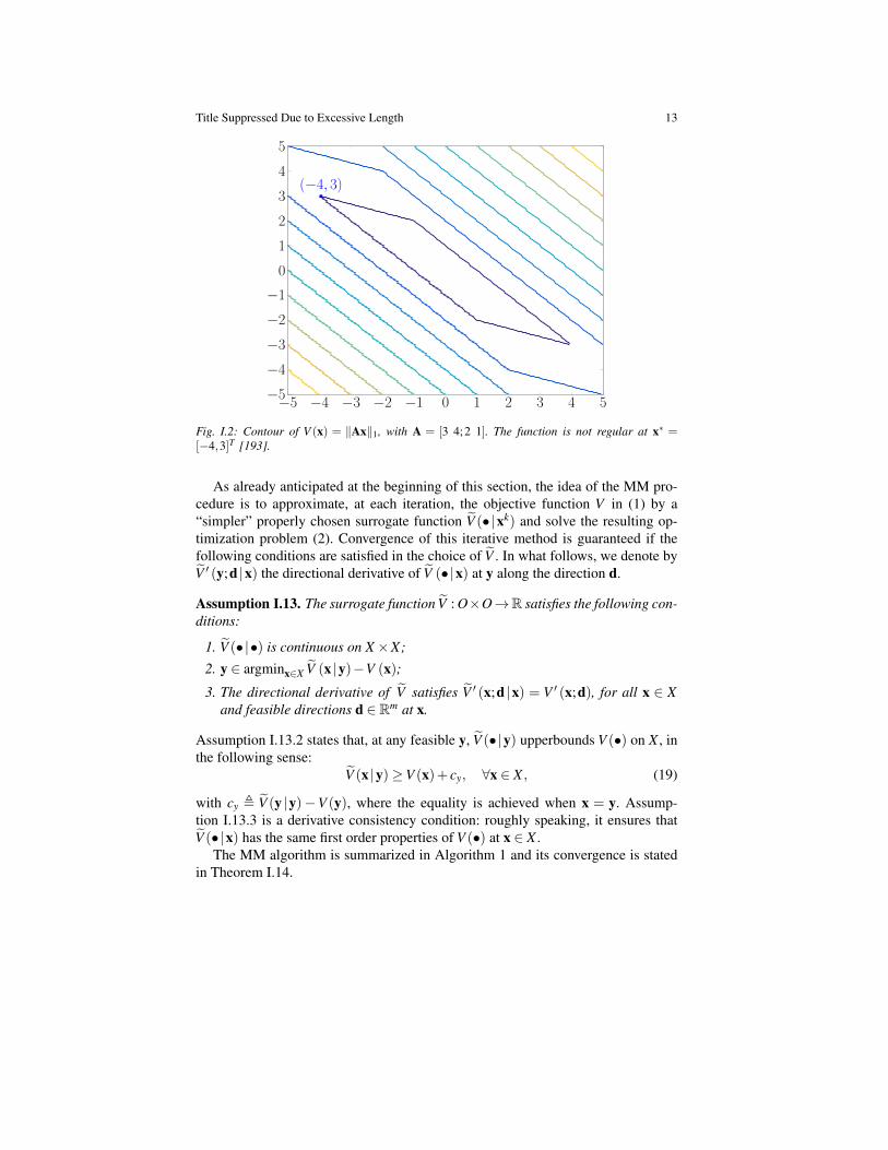
Finally, an example of a nonsmooth, nonseparable function that is not regular isV (x) = ‖Ax‖1, with A = [3 4;2 1] and X = R2. Point x∗ = [−4 3]T is a coordinate-wise d-stationary point, but not d-stationary [cf. Fig. I.2].
I.2. The Majorization-Minimization (MM) AlgorithmWe study Problem (1) under the following blanket assumptions.
Assumption I.12. Given Problem (1), we assume that:
1. X 6= /0 is a closed and convex set in Rm;2. V : O→ R is continuous on the open set O⊇ X;3. V ′(x;d) exists at any x ∈ X and for all feasible directions d ∈ Rm at x;4. V is bounded from below.
Note that the above assumptions are quite standard and are satisfied by most ofthe problems of practical interest; see Sec. I.4 for some illustrative examples.
Title Suppressed Due to Excessive Length 13
−5 −4 −3 −2 −1 0 1 2 3 4 5−5−4−3−2−10
1
2
3
4
5
(−4, 3)
Fig. I.2: Contour of V (x) = ‖Ax‖1, with A = [3 4;2 1]. The function is not regular at x∗ =[−4,3]T [193].
As already anticipated at the beginning of this section, the idea of the MM pro-cedure is to approximate, at each iteration, the objective function V in (1) by a“simpler” properly chosen surrogate function V (•|xk) and solve the resulting op-timization problem (2). Convergence of this iterative method is guaranteed if thefollowing conditions are satisfied in the choice of V . In what follows, we denote byV ′ (y;d |x) the directional derivative of V (•|x) at y along the direction d.
Assumption I.13. The surrogate function V : O×O→R satisfies the following con-ditions:
1. V (•|•) is continuous on X×X;
2. y ∈ argminx∈X V (x |y)−V (x);3. The directional derivative of V satisfies V ′ (x;d |x) = V ′ (x;d), for all x ∈ X
and feasible directions d ∈ Rm at x.
Assumption I.13.2 states that, at any feasible y, V (•|y) upperbounds V (•) on X , inthe following sense:
V (x |y)≥V (x)+ cy, ∀x ∈ X , (19)
with cy , V (y |y)−V (y), where the equality is achieved when x = y. Assump-tion I.13.3 is a derivative consistency condition: roughly speaking, it ensures thatV (•|x) has the same first order properties of V (•) at x ∈ X .
The MM algorithm is summarized in Algorithm 1 and its convergence is statedin Theorem I.14.

14 Gesualdo Scutari and Ying Sun
Algorithm 1: The Majorization-Minimization (MM) Algorithm
Data : x0 ∈ X . Set k = 0.(S.1) : If xk satisfies a termination criterion: STOP;(S.2) : Update x as
xk+1 ∈ argminx∈X
V (x |xk); (20)
(S.3) : k← k+1, and go to (S.1).
Theorem I.14. Let xkk∈N+ be the sequence generated by Algorithm 1 under As-sumptions I.12 and I.13. Then, every limit point of xkk∈N+ (if exists) is a d-stationary solution of Problem (1).
Proof. The main properties of Algorithm 1 is to generate a nonincreasing sequenceV (xk). Indeed, we have
V (xk+1)(19)≤ V (xk+1 |xk)− ck
(20)≤ V (xk |xk)− ck (a)
= V (xk), (21)
where ck , V (xk |xk)−V (xk), and (a) follows from the fact that the inequality (19)is achieved with equality at x = xk.
Let x∗ be a limit point of xkk∈N+ , that is, limt→∞ xkt = x∗ ∈ X . We have
V (xkt+1 |xkt+1)−ckt+1 =V (xkt+1)(21)≤ V (xkt+1)≤ V (xkt+1 |xkt )−ckt ≤ V (x |xkt )−ckt ,
for all x∈ X . Let t→+∞; invoking the continuity of V (•|•) and V (•), we have thatthe sequence cktt∈N+ converges (to a finite value). Therefore,
V (x∗ |x∗)≤ V (x |x∗) , ∀x ∈ X , (22)
which implies
0≤ V ′ (x∗;d |x∗) (a)= V (x∗;d) , ∀d ∈ Rm such that x∗+d ∈ X , (23)
where (a) follows from Assumption I.13.3. This shows that x∗ is a d-stationary so-lution of Problem (1).
Note that, since the sequence V (xk) is nonincreasing, a sufficient condition forxk to admit a limit point is that the set x ∈ X : V (x) ≤ V (x0) is compact. Asufficient condition for that is the coercivity of V on X .
On the termination criterion. We briefly discuss how to choose the termination crite-rion in Step 2 of Algorithm 1; we refer the interested reader to [241] for more details.Let M : X → X be a map such that M(xk) ∈ argminx∈XV (x |xk) and xk+1 = M(xk)
[cf. (2)]. In words, among all the global minimizers of V (•|xk) on X , M uniquelyselects the one, xk+1, used in Step 2 of the MM algorithm. We shown next that

Title Suppressed Due to Excessive Length 15
V (M(x)) =V (x) is a sufficient condition of x being a d-stationary solution of Prob-lem (1). It follows from (21) that V (M(x)) = V (x) forces V (M(x) |x) = V (x |x),which implies that x is a minimizer of V (•|x) on X , and thus (by Assumption I.13.3)a d-stationary point of (1). Based on the above observation and assuming that M(•)is continuous, the following is a valid merit function to measure distance from sta-tionarity of the iterate xk:
Jk+1 ,V (xk)−V (xk+1)
max(1, |V (xk)|) . (24)
The continuity assumption of M maybe hard to check directly. A stronger con-dition implying continuity of M is that the minimizer of V (•|xk) over X is unique,for all xk ∈ X [241, Lemma 1]. Note that, in such a case, it is not difficult to checkthat, if x is a fixed-point of M, then it must be a d-stationary point of Problem (1).Therefore, in the aforementioned setting, an alternative merit function is
Jk+1 , ‖xk+1−xk‖. (25)
Other termination criteria are discussed in Lecture II for SCA-based algorithms.
I.2.1 Discussion on Algorithm 1
The following comments on Algorithm 1 are in order.
On the choice of surrogate functionThe successful application of the MM algorithms relies on the possibility of findinga valid surrogate function V . The critical assumption to be satisfied is undoubt-edly the upperbound condition, as stated in Assumption I.13.2. We provide nextsome systematic rules which help to build a surrogate function that meets this con-dition (and the other required assumptions); several illustrating examples are alsodiscussed. Although for specific (structured) problems it is possible to find a non-convex surrogate function whose minimizer can be computed efficiently, a convexsurrogate is in general preferred, since it leads to a convex subproblem (2). There-fore, next we mainly focus on convex surrogates.1) First order Taylor expansion: Suppose V is a differentiable concave functionon X . A natural choice for V satisfying Assumption I.13 is then: given y ∈ X ,
V (x |y) =V (y)+∇V (y)T (x−y). (26)
More generally, V can be chosen as any convex differentiable function on X , sayVcvx, satisfying the gradient consistency condition ∇Vcvx(x |x) =∇V (x), for all x∈X ; this is enough for Assumption I.13.2 (and thus Assumption I.13) to be satisfied,as shown by the following chain of inequalities
16 Gesualdo Scutari and Ying Sun
V (x)−V (y)(a)≤ ∇V (y)T (x−y)
(b)= ∇Vcvx(y |y)T (x−y)
(c)≤ Vcvx(x |y)−Vcvx(y |y),
(27)where (a) follows from the concavity of V ; in (b) we used ∇Vcvx(y |y) = ∇V (y);and (c) follows from the convexity of Vcvx. Eq. (27) shows that (19) (thus Assump-tion I.13.2) is satisfied by such a Vcvx.
Example 1. V (x) = log(x) is concave on (0,+∞]. Hence, it can be majorized byV (x |y) = x/y, for any given y > 0.
Example 2. V (x) = |x|p, with p ∈ (0,1), is concave on (−∞,0) and (0,+∞). It thuscan be majorized by the quadratic function V (x |y)= p
2 |y|p−2 x2, for any given y 6= 0.
2) Second order Taylor expansion: Suppose V is C1, with L-Lipschitz gradient onX . Then V can be majorized by the surrogate function: given y ∈ X ,
V (x |y) =V (y)+∇V (y)T (x−y)+L2‖x−y‖2. (28)
Moreover, if V is twice differentiable and there exists a matrix M ∈ Rm×m suchthat M−∇2V (x) 0, for all x ∈ X , then V can be majorized by the following validsurrogate function
V (x |y) =V (y)+∇V (y)T (x−y)+12(x−y)T M(x−y). (29)
Example 3 (The proximal gradient algorithm). Suppose that V admits the structureV = F +G, where F : Rm→R is C1, with L-Lipschitz gradient on X , and G : Rm→R is convex (possibly nonsmooth) on X . Using (28) to majorize F , a valid surrogatefor V is: given y ∈ X ,
V (x |y) = F(xk)+∇F(y)T (x−y)+L2‖x−y‖2 +G(x). (30)
Quite interestingly, the above choice leads to a strongly convex subproblem (2),whose minimizer has the following closed form:
xk+1 = prox1/L,G
(xk− 1
L∇F(xk)
), (31)
where proxγ,G(•) is the proximal response, defined as
proxγ,G(x), argminz
G(z)+
12γ‖z−x‖2
.
The resulting MM algorithm (Algorithm 1) turns out to be the renowned proximalgradient algorithm, with step-size γ = 1/L.
3) Pointwise maximum: Suppose V : Rm → R can be written as the pointwisemaximum of functions fiI
i=1, i.e.,

Title Suppressed Due to Excessive Length 17
V (x), maxi=1,...,I
fi(x),
where each fi : Rm → R satisfies Assumption I.12.2 & I.12.3. Then V can be ma-jorized by
V (x |y) = maxi=1,...,I
fi(x |y), (32)
for any given y ∈ X , where fi : X ×X → R is a surrogate function of fi satisfyingAssumption I.13 and fi(y |y)= fi(y). It is not difficult to verify that V above satisfiesAssumption I.13. Indeed, the continuity of V follows from that of fi. Moreover, wehave V (y |y) = V (y). Finally, condition I.13.3 is a direct consequence of LemmaI.8:
V ′(x;d) (13)= max
i∈A(x)f ′i (x;d) = max
i∈A(x)f ′i (x;d |x) = V ′(x;d |x), (33)
where A(x) = i : fi(x) =V (x)= i : fi(x |x) = V (x).4) Composition by a convex function: Suppose V : Rm→ R can be expressed asV (x) , f (∑n
i=1 Aix), where f : Rm → R is a convex function and Ai ∈ Rm×m aregiven matrices. Then, one can construct a surrogate function of V leveraging thefollowing inequality due to convexity of f :
f
(n
∑i=1
wixi
)≤
n
∑i=1
wi f (xi) (34)
for all ∑ni=1 wi = 1 and each wi > 0. Specifically, rewrite first V as: given y ∈ Rm,
V (x) = f
(n
∑i=1
Aix
)= f
(n
∑i=1
wi
(Ai(x−y)
wi+
n
∑i=1
Aiy
)).
Then, using (34) we can upperbound V as
V (x)≤ V (x|y) =n
∑i=1
wi f
(Ai(x−y)
wi+
n
∑i=1
Ai y
). (35)
It is not difficult to check that V satisfies Assumption I.13. Eq. (35) is particularlyuseful to construct surrogate functions that are additively separable in the (block)variables, which opens the way to parallel solution methods wherein (blocks of)variables are updated in parallel. Two examples are discussed next.
Example 4. Let V : Rm→R be convex and let x ∈Rm be partitioned as x = (xi)ni=1,
where xi ∈ Rmi and ∑ni=1 mi = m. Let us rewrite x in terms of its block as x =
∑ni=1 Aix, where Ai ∈ Rm×m is the block diagonal matrix such that Aix = (x)i, with
(x)i , [0T , . . . ,0T , xTi ,0T , . . . ,0T ]T denoting the operator nulling all the blocks of x
except the i-th one. Then using (35) one can choose the following surrogate function:given y = (yi)
ni=1, with each yi ∈ Rmi ,
18 Gesualdo Scutari and Ying Sun
V (x) =V
(n
∑i=1
Aix
)≤ V(x |y),
n
∑i=1
wi V(
1w i
((x)i− (y)i)+y).
It is easy to check that such a V is separable in the blocks xi’s.
Example 5. Let V : R→ R be convex and let vectors x, a ∈ Rm be partitioned asx = (xi)
ni=1 and a = (ai)
ni=1, respectively, with xi and ai having the same size. Then,
invoking (35), a valid surrogate function of the composite function V (aT x) is: giveny = (yi)
ni=1, partitioned according to x,
V (aT x) =V
(n
∑i=1
(a)Ti x
)≤ V (x |y),
n
∑i=1
wi V
((a)T
i (x−y)wi
+n
∑i=1
(a)Ti y
)
=n
∑i=1
wiV(
aTi (xi−yi)
wi+aT y
).
(36)
This is another example of additively (block) separable surrogate function.
5) Surrogates based on special inequalities: Other techniques often used to con-struct valid surrogate functions leverage specific inequalities, such as the Jensen’sinequality, the arithmetic-geometric-mean inequality, and the Cauchy-Schwartz in-equality. The way of using these inequalities, however, depends on the specificexpression of the objective function V under consideration; generalizing these ap-proaches to arbitrary V ’s seems not possible. We provide next two illustrative (non-trivial) case studies based on the Jensen’s inequality and the arithmetic-geometric-mean inequality while we refer the interested reader to [228] for more examplesbuilding on this approach.
Example 6 (The Expectation-Maximization algorithm). Given a pair of random(vector) variables (s,z) whose joint probability distribution p(s,z|x) is parametrizedby x, we consider the maximum likelihood estimation problem of estimating x onlyfrom s while the random variable z is unobserved/hidden. The problem is formulatedas
xML = argminx
V (x),− log p(s|x)
, (37)
where p(s|x) is the (conditional) marginal distribution of s.In general, the expression of p(s|x) is not available in closed form; moreover
numerical evaluations of the integration of p(s,z|x) with respect to z can be com-putationally too costly, especially if the dimension of z is large. In the following weshow how to attach Problem (37) using the MM framework. We build next a validsurrogate function for V leading to a simpler optimization problem to solve.
Specifically, we can rewrite V as
Title Suppressed Due to Excessive Length 19
V (x) =− log p(s|x)
=− log∫
p(s|z,x)p(z|x)dz
=− log∫ ( p(s|z,x)p(z|s,xk)
p(z|s,xk)
)p(z|x)dz
=− log∫ ( p(s|z,x)p(z|x)
p(z|s,xk)
)p(z|s,xk)dz
(a)≤ −
∫log(
p(s|z,x)p(z|x)p(z|s,xk)
)p(z|s,xk)dz
=−∫
log(p(s,z|x)) p(z|s,xk)dz+∫
log(
p(z|s,xk))
p(z|s,xk)dz︸ ︷︷ ︸constant
,
where (a) follows from the Jensen’s inequality. This naturally suggests the followingsurrogate function of V : given y,
V (x |y) =−∫
log(p(s,z|x)) p(z|s,y)dz. (38)
In fact, it is not difficult to check that such a V satisfies Assumption I.13.The update of x resulting from the MM algorithm then reads
xk+1 ∈ argminx
−∫
log(p(s,z|x)) p(z|s,xk)dz. (39)
Problem (39) can be efficiently solved for specific probabilistic models, includingthose belonging to the exponential family, the Gaussian/multinomial mixture model,and the linear Gaussian latent model.
Quite interestingly, the resulting MM algorithm [Algorithm 1 based on the update(39)] turns out to be the renowned Expectation-Maximization (EM) algorithm [66].The EM algorithm starts from an initial estimate x0 and generates a sequence xk byrepeating the following two steps:
• E-step: Calculate V (x |xk) as in (38);• M-step: Update xk+1 as xk+1 ∈ argmaxx−V (x |xk).
Note that these two steps correspond exactly to the majorization and minimiza-tion steps (38) and (39), respectively, showing that the EM algorithm belongs to thefamily of MM schemes, based on the surrogate function (38).
Example 7 (Geometric programming). Consider the problem of minimizing a sig-nomial
V (x) =J
∑j=1
c j
n
∏i=1
xαi ji
on the nonnegative orthant Rn+, with c j,αi j ∈R. In the following, we assume that V
is coercive on Rn+. A sufficient condition for this to hold is that for all i = 1, . . . ,n
20 Gesualdo Scutari and Ying Sun
there exists at least one j such that c j > 0 and αi j > 0, and at least one j such thatc j > 0 and αi j < 0 [136].
We construct a separable surrogate function of V at given y ∈ Rn++. We first
derive an upperbound for the summand in V with c j > 0 and a lowerbound for thosewith c j < 0, using the arithmetic-geometric mean inequality and the concavity ofthe log function (cf. Example 1), respectively.
Let zi and αi be nonnegative scalars, the arithmetic-geometric mean inequalityreads
n
∏i=1
zαii ≤
n
∑i=1
αi
‖ααα‖1z‖ααα‖1i . (40)
Since yi > 0 for all i = 1, . . . ,n, let zi = xi/yi for αi > 0 and zi = yi/xi for αi < 0.Then (40) implies that the monomial ∏
ni=1 xαi
i can be upperbounded on Rn++ as
n
∏i=1
xαii ≤
(n
∏i=1
(yi)αi
)n
∑i=1
|αi|‖ααα‖1
(xi
yi
)‖ααα‖1sign(αi)
. (41)
To upperbound the terms in V with negative c j on Rn++, which is equivalent to
find a lowerbound of ∏ni=1 xαi
i , we use the bound introduced in Example 1, withx = ∏
ni=1 xαi
i , which yields
log
(n
∏i=1
xαii
)≤ log
(n
∏i=1
(yi)αi
)+
(n
∏i=1
(yi)αi
)−1( n
∏i=1
xαii −
n
∏i=1
(yi)αi
).
Rearranging the terms we have
n
∏i=1
xαii ≥
n
∏i=1
(yi)αi
(1+
n
∑i=1
αi logxi−n
∑i=1
αi logyi
). (42)
Combining (41) and (42) leads to the separable surrogate function V (x |y) ,∑
ni=1 Vi(xi |y) of V , with
Vi(xi |y), ∑j:c j>0
c j
(n
∏`=1
(y`)α` j
)|αi j|‖ααα j‖1
(xi
yi
)‖ααα j‖1sign(αi j)
+ ∑j:c j<0
c j
(n
∏`=1
(y`)α` j
)αi j logxi.
(43)
Function V (•|y) is coercive since it is continuous and upperbounds V on Rn++,
therefore xk+1 ∈ Rn++ (recall that we assumed xk ∈ Rn
++). Moreover, the followingchain of inequalities holds:
V (xk+1)≤ V (xk+1 |xk)≤ V (xk |xk) =V (xk)≤ ·· · ≤V (x0)<+∞, (44)
Title Suppressed Due to Excessive Length 21
which implies that, given x0 ∈ R++, the sequence xk generated by the MM algo-rithm always stays in the compact set X0 , x |V (x)≤V (x0) ⊆ Rn
++.As V (x |xk) is separable, xk+1 thus can be computed in parallel. In addition,
focusing on a single component xi and performing the change of variable xi = ezi ,it is not difficult to check that Vi is convex in zi; its global minimizer can be thencomputed efficiently by solving a one dimensional convex optimization problem.
Parallel implementationWhen dealing with large-scale optimization instances of Problem (1), solving sub-problem (2) with respect to the entire x might be either computationally too costlyor practically infeasible. When the feasible set X admits a Cartesian product struc-ture, i.e., X = X1×·· ·×Xn, with Xi ⊆Rmi , a natural approach to cope with the curseof dimensionally is partitioning the vector of variables x into n blocks according toX , i.e., x =
[xT
1 , . . . ,xTn]T and each xi ∈ Rmi , and leveraging a multi-core comput-
ing environment to optimize the blocks in parallel. When using the MM algorithm,a natural way to achieve this goal is to construct a surrogate function V (•|y) thatis additively separable in the blocks, i.e., V (x |y) = ∑
ni=1 Vi(xi |y), so that the sub-
problem (2) can be decoupled in independent optimization problems, one per block.Some of the examples discussed above [cf. (26), (28), (35)] show cases where thiscan be readily achieved by exploring the special structure of the objective functionV . However, when the objective function V does not enjoy any special structure, itseems that there is no general procedure to leverage to obtain a separable surrogatefunction satisfying Assumption I.13. In such cases, a way to cope with the curse ofdimensionality is to solve the subproblem (2) by minimizing the (nonseparable) sur-rogate function block-wise. Such a version of the MM algorithm, termed Block-MM,is discussed in details in the next section.
I.3. The Block Majorization-Minimization Algorithm
In this section, we introduce the Block MM (BMM) algorithm solving Problem (1),whose feasible set is now assumed to have a Cartesian product structure.
Assumption I.15. The feasible set X of Problem (1) admits the Cartesian productstructure X = X1×·· ·×Xn, with each Xi ∈ Rmi and ∑
ni=1 mi = m.
In the above setting, the optimization variables of (1) can be partitioned in (nonover-lapping) blocks xi. When judiciously exploited, this block-structure can lead to low-complexity algorithms that are implementable in a parallel/distributed manner. TheBMM algorithm is a variant of the MM scheme (cf. Algorithm 1) whereby only oneblock of variables is updated at a time. More specifically, at iteration k, a block isselected according to some predetermined rule, say block ik, and updated by solvingthe subproblem
xk+1ik ∈ argmin
xik∈Xik
Vik
(xik |xk
), (45)

22 Gesualdo Scutari and Ying Sun
whereas xk+1j = xk
j, for all j 6= ik. In (45), Vik(•|xk) is a suitably chosen surrogatefunction of V , now function only of the block xik . Conditions on Vik are similarto those already introduced for the MM algorithm (cf. Assumption I.13) and sum-marized below. We use the following notation: Oi ⊆ Rmi is an open set contain-ing Xi and O = O1×·· ·×On; x−i , [xT
1 , . . . ,xTi−1,x
Ti+1, . . . ,x
Tn ]
T denotes the vectorcontaining all the blocks of x but the i-th one; (x)i , [0T , . . . ,0T , xT
i ,0T , . . . ,0T ]T
denotes the operator nulling all the blocks of x except for the i-th one; and with aslight abuse of notation, we use (xi,y−i) to denote the ordered tuple (y1, . . . , yi−1,xi,yi+1, . . . ,yn).
Assumption I.16. Each surrogate function Vi : Oi×O→ R satisfies the followingconditions:
1. Vi(•|•) is continuous on Xi×X;
2. yi ∈ argminxi∈XiVi (xi |y)−V (xi,y−i), for all y ∈ X;
3. The directional derivative of V ′i satisfies V ′i (xi;di |x) =V ′ (x;(d)i), for all xi ∈Xi and feasible directions di ∈ Rmi at xi.
The next question is how to choose the blocks to be updated at each iteration, inorder to have convergence. Any of the following rules can be adopted.
Assumption I.17. Blocks in (45) are chosen according to any of the following rules:
1. Essentially cyclic rule: There exits a finite positive T such that⋃T−1
t=0 ik+t =1, . . . ,n, for all k = 0,1, . . .;
2. Maximum block improvement rule: Choose
ik ∈ argmini=1,...,n
minxi∈Xi
Vi
(xi |xk
);
3. Random-based rule: There exists a pmin > 0 such that P(ik = j|xk−1, . . . ,x0
)=
pkj ≥ pmin, for all j = 1, . . .n and k = 0,1, . . ..
The first two rules above are deterministic rules. Roughly speaking, the essentiallycyclic rule (Assumption I.17.1) states that all the blocks must be updated at leastonce within any T consecutive iterations, with some blocks possibly updated morefrequently than others. Of course, a special case of this rule is the simple cyclic rule,i.e., ik = (k mod n)+1, whereby all the blocks are updated once every T iterations.The maximum block improvement rule (Assumption I.17.2) is a greedy-based up-date: only the block that generates the largest decrease of the surrogates Vi at xk isselected and updated. Finally the random-based selection rule (Assumption I.17.3)selects block randomly and independently, with the condition that all the blockshave a bounded away from zero probability to be chosen. The BMM algorithm issummarized in Algorithm 2.

Title Suppressed Due to Excessive Length 23
Algorithm 2: Block MM Algorithm
Data : x0 ∈ X . Set k = 0.(S.1) : If xk satisfies a termination criterion: STOP;(S.2) : Choose an index ik ∈ 1, . . . ,n;(S.3) : Update xk as
− Set xk+1ik∈ argminxik∈Xik
Vik(xik |xk
);
− Set xk+1j = xk
j, for all j 6= ik;(S.4) : k← k+1, and go to (S.1).
Convergence results of Algorithm 2 consist of two major statements. Under theessential cyclic rule (Assumption I.17.1), quasi convexity of the objective functionis required [along with the uniqueness of the minimizer in (45)], which also guaran-tees the existence of the limit points. This is in the same spirit as the classical proofof convergence of Block Coordinate Descent methods; see, e.g., [14, 214, 250]. Ifthe maximum block improvement rule (Assumption I.17.2) or the random-based se-lection rule (Assumption I.17.3) are used, then a stronger convergence result canbe proved by relaxing the quasi-convexity assumption and imposing the compact-ness of the level sets of V . In order to state the convergence result, we introduce thefollowing additional assumptions.
Assumption I.18. Vi (•|y) is quasi-convex and subproblem (45) has a unique solu-tion, for all y ∈ X.
Assumption I.19. The level set X0 , x ∈ X : V (x)≤V(x0) is compact and sub-
problem (45) has a unique solution for all xk ∈ X and at least n−1 blocks.
We are now ready to state the main convergence result of the BMM algorithm(Algorithm 2), as given in Theorem I.20 below (the statement holds almost surely forthe random-based selection rule). The proof of this theorem can be found in [193];see also Sec. I.5 for a detailed discussion on (other) existing convergence results.
Theorem I.20. Given Problem (1) under Assumptions I.12 and I.15, let xkk∈N+
be the sequence generated by Algorithm 2, with V chosen according to Assump-tion I.16. Suppose that, in addition, either one of the following two conditions issatisfied:
(a) ik is chosen according to the essentially cyclic rule (Assumption I.17.1) and Vfurther satisfies either Assumption I.18 or I.19;
(b) ik is chosen according to the maximum block improvement rule (Assump-tion I.17.2) or the random-based selection rule (Assumption I.17.3).
Then, every limit point of xkk∈N+ is a coordinate-wise d-stationary solution of(1). Furthermore, if V is regular, then every limit point is a d-stationary solution of(1).
24 Gesualdo Scutari and Ying Sun
I.4. ApplicationsIn this section, we show how to apply the (B)MM algorithm to solve some repre-sentative nonconvex problems arising from applications in signal processing, dataanalysis, and communications. More specifically, we consider the following prob-lems: i) Sparse least squares; ii) Nonnegative least squares; iii) Matrix factoriza-tion, including low-rank factorization and dictionary learning; and iv) the multicastbeamforming problem. Our list is by no means exhaustive; it just gives a flavor of thekind of structured nonconvexity and applications which (B)MM can be successfullyapplied to.
I.4.1 Nonconvex Sparse Least SquaresRetrieving a sparse signal from its linear measurements is a fundamental problemin machine learning, signal processing, bioinformatics, physics, etc.; see [269] and[4,97] for a recent overview and some books, respectively, on the subject. Considera linear model, z = Ax+n, where x ∈ Rm is the sparse signal to estimate, z ∈ Rq isthe vector of available measurements, A ∈ Rq×m is the given measurement matrix,and n ∈ Rq is the observation noise. To estimate the sparse signal x, a mainstreamapproach in the literature is to solve the following optimization problem
minimizex
V (x), ‖z−Ax‖2 +λG(x), (46)
where the first term in the objective function measures the model fitness whereas theregularization G is used to promote sparsity in the solution, and the regularizationparameter λ ≥ 0 is chosen to balance the trade-off between the model fitness andsparsity of the solution.
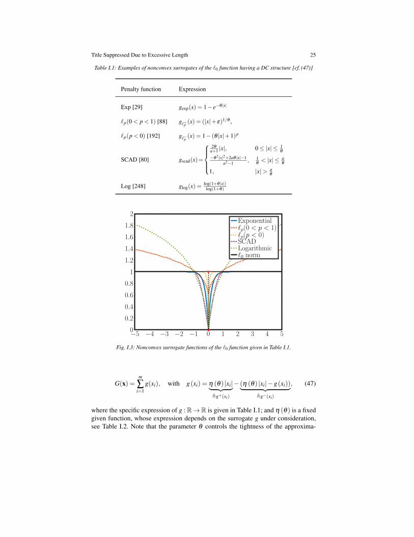
The ideal choice for G would be the cardinality of x, also referred to as `0 “norm”of x. However, its combinatorial nature makes the resulting optimization problemnumerically intractable as the variable dimension m becomes large. Due to its fa-vorable theoretical guarantees (under some regularity conditions on A [33, 34]) andthe existence of efficient solution methods for convex instances of (46), the `1 normhas been widely adopted in the literature as convex surrogate G of the `0 func-tion (in fact, the `1 norm is the convex envelop of the `0 function on [−1,1]m)[30, 235]. Yet there is increasing evidences supporting the use of nonconvex for-mulations to enhance the sparsity of the solution as well as the realism of the mod-els [2,36,94,152,223]. For instance, it is well documented that nonconvex surrogatesof the `0 function, such as the SCAD [80], the “transformed” `1, the logarithmic,the exponential, and the `p penalty [266], outperform the `1 norm in enhancing thesparsity of the solution. Table I.1 summarizes these nonconvex surrogates whereasFig. I.3 shows their graph.
Quite interestingly, it has been recently shown that the aforementioned noncon-vex surrogates of the `0 function enjoy a separable DC (Difference of Convex) struc-ture (see, e.g., [2, 233] and references therein); specifically, we have the following
Title Suppressed Due to Excessive Length 25
Table I.1: Examples of nonconvex surrogates of the `0 function having a DC structure [cf. (47)]
Penalty function Expression
Exp [29] gexp(x) = 1− e−θ |x|
`p(0 < p < 1) [88] g`+p (x) = (|x|+ ε)1/θ ,
`p(p < 0) [192] g`−p (x) = 1− (θ |x|+1)p
SCAD [80] gscad(x)=
2θ
a+1 |x|, 0≤ |x| ≤ 1θ
−θ 2|x|2+2aθ |x|−1a2−1 , 1
θ< |x| ≤ a
θ
1, |x|> aθ
Log [248] glog(x) =log(1+θ |x|)
log(1+θ)
−5 −4 −3 −2 −1 0 1 2 3 4 50
0.2
0.4
0.6
0.8
1
1.2
1.4
1.6
1.8
2Exponential`p(0 < p < 1)`p(p < 0)SCADLogarithmic`0 norm
Fig. I.3: Nonconvex surrogate functions of the `0 function given in Table I.1.
G(x) =m
∑i=1
g(xi), with g(xi) = η (θ) |xi|︸ ︷︷ ︸,g+(xi)
− (η (θ) |xi|−g(xi))︸ ︷︷ ︸,g−(xi)
, (47)
where the specific expression of g : R→R is given in Table I.1; and η (θ) is a fixedgiven function, whose expression depends on the surrogate g under consideration,see Table I.2. Note that the parameter θ controls the tightness of the approxima-

26 Gesualdo Scutari and Ying Sun
Table I.2: Explicit expression of η(θ) and dg−/dx [cf. (47)]
g η(θ) dg−θ/dx
gexp θ sign(x) ·θ · (1− e−θ |x|)
g`+p1θ
ε1/θ−1 1θ
sign(x) · [ε 1θ−1− (|x|+ ε)
1θ−1]
g`−p −p ·θ −sign(x) · p ·θ · [1− (1+θ |x|)p−1]
gscad2θ
a+1
0, |x| ≤ 1
θ
sign(x) · 2θ(θ |x|−1)a2−1 , 1
θ< |x| ≤ a
θ
sign(x) · 2θ
a+1 , otherwise
glogθ
log(1+θ) sign(x) · θ 2|x|log(1+θ)(1+θ |x|)
tion of the `0 function: in fact, it holds that limθ→+∞ g(xi) = 1 if xi 6= 0, otherwiselimθ→+∞ g(xi) = 0. Moreover, it can be shown that for all the functions in TableI.1, g− is convex and has Lipschitz continuous first derivative dg−/dx [233], whoseclosed form is given in Table I.2.
Motivated by the effectiveness of the aforementioned nonconvex surrogates ofthe `0 function and recent works [2, 149, 208, 261, 266], in this section, we showhow to use the MM framework to design efficient algorithms for the solution ofProblem (46), where G is assumed to have the DC structure (47), capturing thus in aunified way all the nonconvex `0 surrogates reported in Table I.1. The key questionis how to construct a valid surrogate function V of V in (46). We address this issuefollowing two steps: 1) We first find a surrogate G for the nonconvex G in (47)satisfying Assumption I.16; and 2) then we construct the overall surrogate V of V ,building on G.Step 1: Surrogate G of G. There are two ways to construct G, namely: i) tailoringG to the specific structure of the function g under consideration (cf. Table I.1); orii) leveraging the DC structure of g in (47) and obtain a unified expression for G,valid for all the DC functions in Table I.1. Few examples based on the approach i)are shown first, followed by the general design as in ii).
Example 8 (The log `0 surrogate). Let G be the “log” `0 surrogate, i.e., G(x) =∑
mi=1 glog(xi), where glog is defined in Table I.1. A valid surrogate is obtained ma-
jorizing the log function glog (cf. Example 1), which leads to G(x |y)=∑mi=1 glog(xi |yi),
withglog(xi |yi) =
θ
log(1+θ)· 1
1+θ |yi||xi|. (48)
Example 9 (The `p(0 < p < 1) surrogate). Let G be the `p(0 < p < 1) function, i.e.,G(x) = ∑
mi=1 g`+p (xi), where g`+p is defined in Table I.1. Similar to the Log surrogate,
Title Suppressed Due to Excessive Length 27
we can derive a majorizer of such a G(x) by exploiting the concavity of g`+p . Wehave
g`+p (xi |yi) =1θ(|yi|+ ε)1/θ−1|xi|. (49)
The desired valid surrogate is then given by G(x |y) = ∑mi=1 g`+p (xi |yi).
Example 10 (DC surrogates). We consider now nonconvex regularizers having theDC structure (47). A natural approach is to keep the convex component g+ in (47)while linearizing the differentiable concave part −g−, which leads to the followingconvex majorizer:
g(xi |yi) = η(θ) |xi|−dg−(x)
dx
∣∣∣∣x=yi
· (xi− yi), (50)
where the expression of dg(x)−/dx is given in Table I.2. The desired majorizationthen reads G(x |y) = ∑
mi=1 g(xi |yi).
Note that although the log and `p surrogates provided in Example 8 and 9 arespecial cases of DC surrogates, the majorizer constructed using (50) is differentfrom the ad-hoc surrogates glog and g`+p in (48) and (49), respectively.
Step 2: Surrogate V of V . We derive now the surrogate of V , when G is given by(47). Since the loss function ‖z−Ax‖2 is convex, two natural options for V are: 1)keeping ‖z−Ax‖2 unaltered while replacing G with the surrogate G discussed inStep 1; or 2) majorizing also ‖z−Ax‖2. The former approach “better” preserves thestructure of the objective function but at the price of a higher cost of each iteration[cf. (2)]: the minimizer of the resulting V does not have a closed form expression;the overall algorithm is thus a double-loop scheme. The latter approach is insteadmotivated by the goal of obtaining low-cost iterations. We discuss next both optionsand establish an interesting connection between the two resulting MM algorithms.• Option 1. Keeping ‖z−Ax‖2 unaltered while using (50), leads to the followingupdate in Algorithm 1:
xk+1 ∈ argminx
V (x |xk), ‖Ax− z‖2 +λ
m
∑i=1
g(xi |xki )
. (51)
Problem (51) is convex but does not have a closed form solution. To solve (51), wedevelop next an ad-hoc iterative soft-thresholding-based algorithm invoking againthe MM framework on V (•|xk) in (51).
We denote by xk,r the r-th iterate of the (inner loop) MM algorithm ( Algo-rithm 1) used to solve (51); we initialize the inner algorithm by xk,0 = xk. Since thequadratic term ‖Ax−z‖2 in (51) has Lipschitz gradient, a natural surrogate functionfor V (x |xk), is [cf. (28)]: given xk,r,
V k(x | xk,r) = 2xT AT (Axk,r− z)+L2‖x−xk,r‖2 +λ
m
∑i=1
g(xi |xki ), (52)
28 Gesualdo Scutari and Ying Sun
where L = 2λmax(AT A). Denoting
bk,r , xk,r− 2L
AT (Axk,r− z)+λ
L·(
dg−(x)dx
∣∣∣∣x=xk
i
)m
i=1
,
the main update of the inner MM algorithm minimizing V k(x | xk,r) reads
xk,r+1 = argminx
L2‖x−bk,r‖2 +λ η(θ)‖x‖1. (53)
Quite interestingly, the solution of Problem (53) can be obtained in closed form.Writing the first order optimality condition
0 ∈ (x−bk,r)+λ η(θ)
L∂‖x‖1,
and recall that the subgradient of ‖x‖1 takes the following form [cf. (10)]:
∂‖x‖1 = ζζζ : ζζζT x = ‖x‖1, ‖ζζζ‖∞ ≤ 1,
we have the following expression for xk,r+1:
xk,r+1 = sign(bk,r) ·max|bk,r|− λ η(θ)
L,0,
where the sign and max operators are applied component-wise. Introducing the soft-thresholding operator
Sα(x), sign(x) ·max|x|−α,0, (54)
xk,r+1 can be rewritten succinctly as
xk,r+1 = S λ η(θ)L
(bk,r), (55)
where the soft-thresholding operator is applied component-wise.Overall the double loop algorithm, based on the MM outer updates (51) and MM
inner iterates (55) is summarized in Algorithm 3.

Title Suppressed Due to Excessive Length 29
Algorithm 3: MM Algorithm for Nonconvex Sparse Least Squares
Data : x0 ∈ X . Set k = 0.(S.1) : If xk satisfies a termination criterion: STOP;(S.2) : Set r = 0. Initialize xk,0 as xk,0 = xk;(S.3) : If xk,r satisfies a termination criterion: STOP;
(a) : Update xk,r as
xk,r+1 = S λ η(θ)L
(bk,r)
;
(b) : r← r+1, and go to (S.3).(S.4) : xk+1 = xk,r, k← k+1, and go to (S.1).
Termination criteria: As the termination criterion of Step 1 and Step 3 in Algo-rithm 3, one can use any valid merit function measuring the distance of the iteratesfrom stationarity of (46) and optimality of (53), respectively. For both the inner andouter loop, it is not difficult to check that the objective functions of the associatedoptimization problems−(53) and (51), respectively−are strictly convex if λ > 0;therefore both optimization problem have unique minimizers. It turns out that bothfunctions defined in (24) and (25) can be adopted as valid merit functions. The loopcan be then terminated once the value of the chosen function goes below the desiredthreshold.• Option 2. Algorithm 3 is a double loop MM-based algorithm: in the outer loop,the surrogate function V (• | xk) [cf. (51)] is iteratively minimized by means of aninner MM algorithm based on the surrogate function V k(x | xk,r) [cf. (52)]. A closedlook at (51) and (52) shows that the following relationship holds between V and V k:
V k(x |xk,0)≥ V (x |xk)≥V (x).
The above inequality shows that V k,0(x |xk) is in fact a valid surrogate function ofV at x = xk. This means that the inner loop of Algorithm 3 can be terminated afterone iteration without affecting the convergence of the scheme. Specifically, Step 3of Algorithm 3 can be replaced with the following iterate
xk+1 = S λ η(θ)L
(bk,0). (56)
The resulting algorithm is in fact an MM scheme minimizing V k,0(•|xk), whoseconvergence is guaranteed by Theorem I.14.
I.4.2 Nonnegative Least Squares
Finding a nonnegative solution x ∈Rm of the linear model z = Ax+n has attractedsignificant attention in the literature. This problem arises in applications where themeasured data is nonnegative; examples include image pixel intensity, economi-cal quantities such as stock price and trading volume, biomedical records such as
30 Gesualdo Scutari and Ying Sun
weight, height, blood pressure, etc [73,139,212]. It is also one of the key ingredientsin nonnegative matrix/tensor factorization problem for analysing structured data set.The nonnegative least squares (NNLS) problem consists in finding a nonnegative xthat minimizes the residual error between the data and the model in least squaresense:
minimizex
V (x), ‖z−Ax‖2
subject to x≥ 0,(57)
where z ∈ Rq and Aq×m are given.Note that Problem (57) is convex. We show next how to construct a surrogate
function satisfying Assumption I.13 which is additively separable in the componentsof x, so that the resulting subproblems (2) can be solved in parallel. To this end, weexpand the square in the objective function and write
V (x) = xT AT Ax−2zT Ax+ zT z. (58)
Let M AAT . Using (29), we can majorize V by
V (x |y) =V (y)+2(AT Ay−AT z)T (x−y)+(x−y)T M(x−y), (59)
for any given y ∈ Rm. The goal is then finding a matrix M AAT that is diago-nal, so that V (x |y) becomes additively separable. We provide next two alternativeexpressions for M.• Option 1: Since ∇V is Lipschitz continuous on Rm, we can use the same up-perbound as in Example 3. This corresponds to choose M = λ I, with λ such thatλ ≥ λmax
(AT A
). This leads overall to the following surrogate of V :
V (x |y) =V (y)+2(AT Ay−AT z)T (x−y)+λ‖x−y‖2.
The above choice leads to a strongly convex subproblem (2), whose minimizer hasthe following closed form:
xk+1 =
[xk− 1
λ
(AT Axk−AT z
)]+
, (60)
where [•]+ denotes the Euclidean projection onto the nonnegative orthant. The re-sulting MM algorithm (Algorithm 1) based on the update (60) turns out to be therenowned gradient projection algorithm with constant step-size 1/λ .•Option 2: If Problem (57) has some extra structure, the surrogate V can be tailoredto V even further. For instance, suppose that in addition to the structure above, therehold A ∈Rq×m
++ , z ∈Rq+ and z 6= 0. It has been shown in [58,139] that the following
diagonal matrix
M, Diag((AT Ay)1
y1, · · · , (A
T Ay)m
ym
)(61)

Title Suppressed Due to Excessive Length 31
satisfies MAT A. Substituting (61) in (59), one obtains the following closed formsolution of the resulting subproblem (2):
xk+1 = (AT z/AT Axk) ·xk,
wherein both division and multiplication are intended to be applied element-wise.
I.4.3 Sparse plus Low-Rank Matrix Decomposition
Another useful paradigm is to decompose a partly or fully observed data matrixinto the sum of a low rank and (bilinear) sparse term; the low-rank component cap-tures correlations and periodic trends in the data whereas the bilinear term explainsparsimoniously data patterns, (co-)clusters, innovations or outliers.
Let Y ∈ Rm×t(m ≤ t) be the data matrix. The goal is to find a low rank matrixL ∈ Rm×t with rank r0 , rank(L) m, and a sparse matrix S ∈ Rm×t such thatY = L+S+V, where V ∈Rm×t accounts for measurement errors. To cope with themissing data in Y, we introduce i) the set Ω ⊆ M×T of index pairs (i, j), whereM , 1, . . . ,m and T , 1, . . . , t; and ii) the sampling operator PΩ (·), which nullsthe entries of its matrix argument not in Ω , leaving the rest unchanged. In this way,one can express incomplete and (possibly noise-)corrupted data as
PΩ (Y)≈ PΩ (L+S), (62)
where ≈ is quantified by a specific loss function (and regularization) [219].Model (62) subsumes a variety of statistical learning paradigms including: (ro-
bust) principal component analysis [32, 41], compressive sampling [35], dictionarylearning (DL) [75, 178], non-negative matrix factorization [107, 122, 138], matrixcompletion, and their robust counterparts [112]. Task (62) also emerges in variousapplications such as (i) network anomaly detection [130, 154, 155]; (i) distributedacoustic signal processing [71, 72]; (iii) distributed localization and sensor iden-tification [205]; (iv) distributed seismic forward modeling in geological applica-tions [171, 271] (e.g., finding the Green’s function of some model of a portion ofthe earth’s surface); (v) topic modeling for text corpus from social media [198,267];(vi) data and graph clustering [98, 126, 127, 236]; and (vii) power grid state estima-tion [93, 120].
In the following, we study task (62) adopting the least-squares (LS) error as lossfunction for ≈. We show in detail how to design an MM algorithm for the solutionof two classes of problems under (62), namely: i) the low-rank matrix completionproblem; and ii) the dictionary learning problem. Similar techniques can be usedalso to solve other tasks modeled by (62).1) Low-rank matrix completion. The low-rank matrix completion problem arisesfrequently in learning problems where the task is to fill in the blanks in the partiallyobserved collinear data. For instance, in movie rating problems, Y is the rating ma-trix whose entries yi j represent the score of movie j given by individual i if he/shehas watched it, and considered missing otherwise. Despite of being highly incom-plete, such a data set is also rank deficient as individuals sharing similar interests

32 Gesualdo Scutari and Ying Sun
may give similar ratings (the corresponding rows of Y are collinear), which makesthe matrix completion task possible. Considering model (62), the question becomeshow to impose a low-rank structure on L and sparse structure on S. We describenext two widely used approaches.
A first approach is enforcing a low-rank structure on L by promoting sparsity onthe singular values of L [denoted by σi(L), i = 1, . . . ,m] as well as on the elementsof S via regularization. This leads to the following formulation
minimizeL,S
V (L,S), ‖PΩ (Y−L−S)‖2F +λr ·Gr(L)+λs ·Gs(S), (63)
where Gr(L), ∑mi=1 gr (σi (L)) and Gs(S), ∑
ri=1 ∑
tj=1 gs (si j) are sparsity promot-
ing regularizers, and λr and λs positive coefficients. Since Gr(L) promotes sparsityon the singular values of L, this will induce a low-rank structure on L. Note that thegeneral formulation (63) contains many popular choices of low-rank inducing penal-ties. For instance, choosing gr(x) = gs(x) = card(x), one gets Gr(L) = rank(L) andGs(S) = ‖S‖0 , ‖vec(S)‖0, which become the exact (nonconvex) rank penalty on Land the cardinality penalty on S, respectively. Another popular choice is gr(x) = |x|,which leads to the convex nuclear norm penalty Gr(L) = ‖L‖∗; another exampleis gr(x) = log(x), which yields the nonconvex logdet penalty. To keep the analy-sis general, in the following we tacitly assume that gr and gs are any of the DCsurrogate functions of the `0 function introduced in Sec. I.4.1 [cf. (47)]. Note that,since gr and gs are DC and σi(L) is a convex function of L, they are all directionallydifferentiable (cf. Sec. I.1). Therefore, V (L,S) in (63) is directionally differentiable.
A second approach to enforce a low-rank structure on L is to “hard-wire” a rank(at most) r into the structure of L by decomposing L as L = DX, where D ∈ Rm×r
and X ∈ Rr×t are two “thin” matrices. The problem then reads
minimizeD,X
‖PΩ (Y−DX−S)‖2F +λr ·Gr(D,X)+λs ·Gs(S), (64)
where Gr and Gs promote low-rank and sparsity structures, respectively. While Gscan be chosen as in (63), the choice of Gr acting on the two factors D and X whileimposing the low-rankness of L is less obvious; two alternative choices are the fol-lowing. Since
‖L‖∗ = infDX=L
12(‖D‖2
F +‖X‖2F),
an option is choosing
Gr(D,X) =12(‖D‖2
F +‖X‖2F).
Another low-rank inducing regularizer is the max-norm penalty
‖L‖max , infDX=L
‖D‖2,∞ +‖X‖2,∞,
where ‖•‖2,∞ denotes the maximum `2 row norm of a matrix; this leads to
Title Suppressed Due to Excessive Length 33
Gr(D,X) = ‖D‖2,∞ +‖X‖2,∞.
Here we focus only on the first formulation, Problem (63); the algorithmic designfor (64) will be addressed within the context of the dictionary learning problem,which is the subject of the next section.
To deal with Problem (63), the first step is to rewrite the objective function ina more convenient form, by getting rid of the projection operator PΩ . Define Q ,diag(q), with qi = 1 if
(vec(PΩ (Y)
))i 6= 0; and qi = 0 otherwise. Then, V (L,S) in
(63) can be rewritten as
V (L,S) = ‖vec(Y)−vec(L+S)‖2Q︸ ︷︷ ︸
Q(L,S)
+λr ·Gr(L)+λs ·Gs(S), (65)
where ‖x‖2Q , xT Qx. Note that since qi is equal to either 0 or 1, we have λmax (Q) =
1. In the following, we derive an algorithm that alternately optimizes L and S basedon the block MM algorithm described in Algorithm 2. In the following, we denoteby mi j the (i, j)-th entry of a generic matrix M.
We start with the optimization of S, given L = Lk. One can easily see thatV (Lk,S) is of the same form as the objective function in Problem (46). Therefore,two valid surrogate functions can be readily constructed using the same techniquealready introduced in Sec. I.4.1. Specifically, two alternative surrogates of V (Lk,S)are [cf. (51)]: given Sk,
V (1)(Lk,S |Sk) = Q(Lk,S)+λs
r
∑i=1
t
∑j=1
gs(si j |ski j) (66)
and [cf. (52)]
V (2)(Lk,S |Sk)
= Q(Lk,Sk)+2(
vec(Y−Lk)−vec(Sk))T
Q(
vec(Y−Lk)−vec(S))
+∥∥∥vec(S)−vec(Sk)
∥∥∥2+λs
r
∑i=1
t
∑j=1
gs(si j |ski j)
=∥∥∥S− Yk− (λs/2) ·Wk
∥∥∥2
F+λs η(θ)‖S‖1 + const.,
(67)
where Wk and Yk are matrices of the same size of S, with (i, j)-th entries defined as
wki j ,
dg−s (x)dx
∣∣∣∣x=sk
i j
and yki j ,
yi j− `k
i j, if (i, j) ∈Ω ,
ski j, otherwise,
(68)
respectively; and in const. we absorbed irrelevant constant terms.The minimizer of V (1)(Lk,•|Sk) and V (2)(Lk,•|Sk) can be computed following
the same steps as described in Option 1 and Option 2 in Sec. I.4.2, respectively.

34 Gesualdo Scutari and Ying Sun
Next, we only provide the update of S based on minimizing V (2)(Lk,•|Sk), whichis given by
sk+1i j = sign
(yi j +(λs/2) ·wk
i j
)·max
∣∣∣yi j +(λs/2) ·wki j
∣∣∣−η(θ)/2,0. (69)
Next, we fix S = Sk+1 and optimize L. In order to obtain a closed form update ofL, we upperbound Q(•,Sk+1) and Gr(•) in (65) using (28) and (26), respectively,and following similar steps as to obtain (67). Specifically, a surrogate of Q(•,Sk+1)is: given Lk,
Q(L,Sk+1 |Lk) = ‖L−Xk‖2F + const., (70)
where Xk is a matrix having the same size of Y, with entries defined as
xki j ,
yi j− sk+1
i j , (i, j) ∈Ω ;`k
i j, otherwise.(71)
To upperbound the nonconvex regularizer Gr(L) = ∑mi=1 g(σi (L)), we invoke (50)
and obtain
gr
(σi(L) |σi(Lk)
)= η(θ)|σi (L) |−wk
i ·(
σi (L)−σi(Lk)), (72)
with
wki ,
dg−r (x)dx
∣∣∣∣x=σi(Lk)
.
Using the directional differentiability of the singular values σi(Lk) (see, e.g., [95])and the chain rule, it is not difficult to check that Assumption I.13 (in particularthe directional derivative consistency condition I.13.3) is satisfied for gr; thereforegr(•|σi(Lk)
)is a valid surrogate function of gr.
Combining (70) and (72) yields the following surrogate function of V (L,Sk+1):
V(
L,Sk+1 |Lk)= ‖L−Xk‖2
F +λr
m
∑i=1
(η |σi (L) |−wk
i σi (L)). (73)
The final step is computing the minimizer of V (L |Lk). To this end, we first intro-duce the following lemma [244].
Lemma I.21 (von Neumann’s trace inequality). Let A and B be two m× mcomplex-valued matrices with singular values σ1(A) ≥ ·· · ≥ σm(A) and σ1(B) ≥·· · ≥ σm(B), respectively. Then,
|Tr(AB)| ≤m
∑i=1
σi(A)σi(B). (74)
Note that Lemma I.21 can be readily generalized to rectangular matrices. Specifi-cally, given A, BT ∈ Rm×t , define the augmented square matrices A, [A;0(t−m)×t ]
and B, [B,0t×(t−m)], respectively. Applying Lemma I.21 to A and B, we get
Title Suppressed Due to Excessive Length 35
Tr(AB) = Tr(AB)≤t
∑i=1
σi(A)σi(B) =m
∑i=1
σi(A)σi(B), (75)
where equality is achieved when A and BT share the same singular vectors. Using(75), we can now derive the closed form of the minimizer of (73).
Proposition I.22. Let Xk = UXΣΣΣ X VTX be the singular value decomposition (SVD) of
Xk. The minimizer of V(L,Sk+1 |Lk
)in (73) (and thus the update of L) is given by
Lk+1 = UX D ηλr2
(ΣΣΣ X +Diag(wk
i λr/2mi=1)
)VT
X , (76)
where Dα (ΣΣΣ) denotes a diagonal matrix with the i-th diagonal element equal to(ΣΣΣ ii−α)+, and (x)+ ,max(0,x).
Proof. Expanding the squares we rewrite V(L,Sk+1 |Lk
)as
V (L,Sk+1 |Lk)
= Tr(LLT )−2Tr(L(Xk)T )+Tr(Xk(Xk)T )+λr
m
∑i=1
(η |σi (L) |−wk
i σi (L))
=m
∑i=1
σ2i (L)−2Tr(L(Xk)T )+λr
m
∑i=1
(η |σi (L) |−wk
i σi (L))+Tr(Xk(Xk)T ).
(77)To find a minimizer of V (•,Sk+1 |Lk), we introduce the SVD of L = ULΣΣΣ LVT
L ,and optimize separately on UL, VL, and ΣΣΣ L, with ΣΣΣ L = diag(σ1(L), . . . ,σm(L)).
From (75) we have Tr(L(Xk)T ) ≤ ∑mi=1 σi(L)σi(Xk), and equality is reached if
UL = UX and VL = VX , respectively; which are thus optimal. To compute the op-timal ΣΣΣ L let us substitute UL = UX and VL = VX in (77) and solve the resultingminimization problem with respect to ΣΣΣ L:
minimizeσi(L)mi=1
m
∑i=1
σi(L)2−2m
∑i=1
σi(L)σi(Xk)+λr
m
∑i=1
(ησi (L)−wk
i σi (L))
subject to σi(L)≥ 0, ∀i = 1, . . . ,m.
(78)
Problem (78) is additively separable. The optimal value of each σi(L) is
σ?i (L) = argmin
σi(L)≥0(σi(L)−σi(Xk)−wk
i λr/2+ηλr/2)2
= (σi(Xk)+wki λr/2−ηλr/2)+,
(79)
which completes the proof.
The block MM algorithm solving the matrix completion Problem (63), based onthe S-updates (69) and L-update (76), is summarized in Algorithm 4.
36 Gesualdo Scutari and Ying Sun
Algorithm 4: Block MM Algorithm for Matrix Completion [cf. (63)]
Data : L0,S0 ∈ Rm×t . Set k = 0.(S.1) : If Lk and Sk satisfy a termination criterion: STOP;(S.2) : Alternately optimize S and L:
(a) : Update Sk+1 as according to (69);(b) : Update Lk+1 according to (76);
(S.3) : k← k+1, and go to (S.1).
2) Dictionary Learning. Given the data matrix Y ∈ Rm×t , the dictionary learning(DL) problem consists in finding a basis, the dictionary D ∈ Rm×r (with r t),over which Y can be sparsely represented throughout the coefficients X ∈ Rr×t .This problem appears in a wide range of machine learning applications, such asimage denoising, video surveillance, face recognition, and unsupervised clustering.We consider the following formulation for the DL problem:
minimizeX,D∈D
V (D,X), ‖Y−DX‖2F︸ ︷︷ ︸
F(D,X)
+λs G(X),(80)
where D is a convex compact set, bounding the elements of the dictionary so thatthe optimal solution will not go to infinity due to scaling ambiguity; and G aims atpromoting sparsity on X, with λs being a positive given constant. In the following,we assume that G(X) = ∑
ri=1 ∑
tj=1 g(xi j), with g being any of the DC functions
introduced in (47).Since F(D,X) in (80) is biconvex, we can derive an algorithm for Problem (80)
based on the block MM algorithm by updating D and X alternately.Given X = Xk, F(D,Xk) is convex in D. A natural choice for a surrogate of
F(D,Xk) is F(D,Xk) itself, that is,
F(1)(D |Xk), F(D,Xk) = ‖Y−DXk‖2F , (81)
and update D solvingDk+1 = argmin
D∈D‖Y−DXk‖2
F . (82)
Problem (82) is convex, but does not have a closed form solution for a generalconstraint set D. In some special cases, efficient iterative method can be derived tosolve (82) by exploiting its structure (see, e.g., [194]). For instance, consider theconstraint set D = D ∈ Rm×r : ‖D‖2
F ≤ α. Writing the KKT conditions of (82)(note that Slater’s constraint qualification holds), we get
0≤ α−‖D‖2F ⊥ µ ≥ 0, (83a)
∇DL(D,µ) = 0, (83b)
where L(D,µ) is the Lagragian function, defined as
Title Suppressed Due to Excessive Length 37
L(D,µ) = ‖Y−DXk‖2F +µ(‖D‖2
F −α). (84)
For any given µ ≥ 0, the solution of (83b) is given by
D(µ) = Y(Xk)T (Xk(Xk)T +µI)−1, (85)
where µ needs to be chosen in order to satisfy the complementarity condition in(83)
0≤ h(µ)⊥ µ ≥ 0, (86)
with h(µ) , α −‖D(µ)‖2F . Since h(•) is monotone, (86) can be efficiently solved
using bisection.An alternative surrogate function of F(D,Xk) leading to a closed form solution of
the resulting minimization problem can be readily obtained leveraging the Lipschitzcontinuity of ∇DF(D,Xk) and using (28), which yields
F(2)(D,Xk |Dk) = 2Tr(DkXkXkT −YXkT )T (D−Dk)
+L‖D−Dk‖2
F + const.,(87)
where L, λmax(SkSkT ) and const. is an irrelevant constant. The update of D is thengiven by
Dk+1 = PD
(1L(DkXkXkT −YXkT )
), argmin
D∈D
∥∥∥∥D−(Dk− 1
L(DkXkXkT −YXkT )
)∥∥∥∥2
,
(88)
which has a closed form expression for simple constraint sets such as D = Rm×r+ ,
D = D |D ∈ Rm×r+ ,‖D‖2
F ≤ α, and D = D |‖di‖22 ≤ αi, ∀i = 1, . . . ,m.
We fix now D = Dk+1, and update X. Problem (80) is separable in the columnsof X; the subproblem associated with the j-th column of X, denoted by x j, reads
xk+1j ∈ argmin
x j
12‖y j−Dk+1x j‖2 +λs
t
∑j=1
gs(xi j). (89)
Note that Problem (89) is of the same form of (46); therefore, it can be solved usingthe MM algorithm, based on the surrogate functions derived in Sec. I.4.1 [cf. (51)and (52)].
I.4.4 Multicast Beamforming
We study the Max-Min Fair (MMF) beamforming problem for single group multi-casting [218], where a single base station (BS) equipped with m antennas wishes totransmit common information to a group of q single-antenna users over the samefrequency band. The goal of multicast beamforming is to exploit the channels andthe spatial diversity offered by the multiple transmit antennas to steer transmitted
38 Gesualdo Scutari and Ying Sun
power towards the group of desired users while limiting interference (leakage) tonearby co-channel users and systems.
Denoting by w ∈ Cm the beamforming vector, the Max-Min beamforming prob-lem reads
maximizew∈Cm
mini=1,...,q
wHRiw
subject to ‖w‖2 ≤ PT ,(90)
where PT is the power budget of the BS and Ri ∈ Cm×m is a positive semidefinitematrix modeling the channel between the BS and user i. Specifically, Ri = hihH
i /σ2i
if instantaneous Channel State Information (CSI) is assumed, where hi is thefrequency-flat quasi-static channel vector from the BS to user i and σ2
i is the vari-ance of the zero-mean, wide-sense stationary additive noise at the i-th receiver; andRi = EhihH
i /σ2i represents the spatial correlation matrix if only long-term CSI is
available (in the latter case, no special structure for Ri is assumed).Problem (90) contains complex variables. One could reformulate the problem
into the real domain by using separate variables for the real and imaginary parts ofthe complex variables, but this approach is not advisable because it does not takeadvantage of the structure of (real) functions of the complex variables. Followinga well-established path in the signal processing and communication communities,here we work directly with complex variables by means of “Wirtinger derivatives”.The main advantage of this approach is that we can use the so-called “Wirtingercalculus” to easily compute in practice derivatives of the functions in (90) directlyin the complex domain. It can be shown that all the results in this chapter extend tothe complex domain when using Wirtinger derivatives instead of classical gradients.Throughout the chapter we will freely use the Wirtinger calculus and refer the readerto [103, 124, 209] for more information on this topic.
We derive now an MM algorithm to solve Problem (90). To do so, we first rewrite(90) in the equivalent minimization form
minimizew∈Cm
maxi=1,...,q
−wHRiw
subject to ‖w‖2 ≤ PT .
Since fi(w),−wHRiw is a concave function on Cm, it can be majorized by itsfirst order approximation: given y ∈ Cm,
fi(w |y) = fi(y)+2Re(y)HRi(w−y)
. (91)
Using (91) and (32), it is easy to check that the following convex function is avalid surrogate of V (w),maxi=1,...,q−wHRiw:
V (w |y) = maxi=1,...,q
fi(w;y). (92)
The main iterate of the MM algorithm based on (92) is then given by: given wk,

Title Suppressed Due to Excessive Length 39
xk+1 ∈ argmin‖w‖2≤PT
max
i=1,...,q−wkHRiwk +2RewkHRi(w−wk)
. (93)
Convergence to d-stationary solutions of (90) is guaranteed by Theorem I.14.

40 Gesualdo Scutari and Ying Sun
I.5. Sources and NotesA bit of history. The MM algorithmic framework has a long history that tracesback to 1970, when the majorization principle was introduced [179] for descent-based algorithms, using line search. In 1977, the MM principle was applied to mul-tidimensional scaling [62,65]. Concurrently, its close relative, the (generalized) EMalgorithm [66], was proposed by Dempster et. al. in 1977 in the context of maximumlikelihood estimation with missing observations. The authors proved the monotonic-ity of the EM scheme showing that the E-step generates an upperbound of the ob-jective function. The idea of successively minimizing an upperbound of the originalfunction appeared in subsequent works, including [63, 90, 91, 134, 188], to name afew; and it was introduced as a general algorithmic framework in [64, 99, 135]. Theconnection between EM and MM was clarified in [10], where the authors arguedthat the majorization step (also referred to as “optimization transfer”) rather thanthe missing data is the key ingredient of EM. The EM/MM algorithm has gainedsignificant attention and applied in various fields ever since [108, 159, 254]. A re-cent tutorial on the MM algorithm along with its applications to problems in signalprocessing, communications, and machine learning can be found in [228].
Building on the plain MM/EM, as described in Algorithm 1, several general-izations of the algorithm have been developed to improve its convergence speed,practical implementability, as well as scalability. Some representative examples arethe following. Both the majorization and minimization steps can be performed in-exactly: the global upperbound condition of the surrogate function can be relaxedto be just a local upperbound; and the exact minimizer of the surrogate functioncan be replaced by one that only decreases the value of the surrogate with respectto the current iterate [66, 131]. MM can also be coupled with line-search schemesto accelerate its convergence [6, 100, 141, 200]. Furthermore, instead of majoriz-ing the objective function on the whole space, the “subspace MM” algorithm con-structs majorizers on an iteration-dependent subspace [47–49, 129]. For structuredproblems whose variables are naturally partitioned in blocks, majorization can bedone block-wise to reduce the scale of the subproblems and achieving tighter up-perbounds [81]. Sweeping rules of the blocks such as the (essential-)cyclic rule,random-based rule, Gauss-Southwell rule, maximum improvement rule, have beenstudied in [81, 111, 193]. An incremental MM was proposed in [151] to minimizesum-utilities composed of a large number of cost functions.On the convergence of MM/EM. Due to the intimacy between MM and EM, con-vergence results of MM cannot be summarized independently from those of EM.Therefore, in the following we will not distinguish between EM and MM. Earlierstudies including the proof of monotonicity of the sequence of the objective valuesalong with the characterization of the limit points of the sequence generated my theEM/MM algorithm were presented in [66]. Results were refined in [27, 252], underthe assumption that the objective function is differentiable and the iterates lie in theinterior of the constraint set: it was shown that, if the surrogate function satisfiessome mild conditions, all the limit points of the sequence generated by the EM/MMalgorithm are stationary points of the problem. Conditions for the convergence of
Title Suppressed Due to Excessive Length 41
the whole sequence were given in [241]. A more comprehensive study of MM con-vergence with extensions to constrained problems and block-wise updates, can befound in [82,111], where the surrogate only needs to upperbound the objective func-tion locally. Convergence of (block-)MM applied to problems with non-smooth ob-jective functions was studied in [193] (cf. Theorem I.14 and I.20). All the aboveresults considered convex constraints. Convergence of MM under non-convex con-straint were only partially investigated; examples include [220] and [59, 157, 263],the latter focusing on specific problems. In many applications, the EM/MM hasbeen observed to be slow [108, 254]. Accelerated versions of EM/MM include:i) [6, 100, 141, 200], based on modifying the step-size; ii) [26, 115, 131, 132, 161],based on adjusting the search direction or inexact computation of the M-step; iii)and [150, 242, 273] based on finding a fixed-point of the algorithmic mapping. Werefer the readers to [116, 159, 228] for a comprehensive overview.On the choice of surrogate function and related algorithms. The performance ofMM depends crucially on the choice of the surrogate function. On one hand, a de-sirable surrogate function should be sufficiently “simple” so that the resulting mini-mization step can be carried out efficiently; on the other hand, it should also preservethe structure of the objective function, which is expected to enhance the practicalconvergence. Achieving a trade-off between these two goals is often a non-trivialtask. Some guidelines on how to construct valid surrogate functions along with sev-eral examples were provided in [108, 151, 254]. Quite interestingly, under specificchoices of the surrogate function, the resulting (block-)MM algorithm becomes aninstance of well-knowns schemes, widely studied in the literature. Examples includethe EM algorithm [66], the convex-concave procedure (CCCP) [145, 191, 264], theproximal algorithms [8, 15, 50, 53, 182], the cyclic minimization algorithm [226],and block coordinate descent-based schemes [250]. Finally, the idea of approximat-ing a function using an upperbound has also been adopted to convexify nonconvexconstraint functions; examples include the inner approximation algorithm [158], theCCCP procedure, and SCA-based algorithms [77, 207, 208].Applications of MM/EM. In the last few years there has been a growing inter-est in using the MM framework to solve a gamut of problems in several fields,including signal/image processing, machine learning, communications, and bioin-formatics, just to name a few. A non-exhaustive list of specific applications includesparse linear/logistic regression [7, 21, 23, 36, 59, 85, 86, 125, 156], sparse (general-ized) principal component analysis [118,221,263], matrix factorization/completion[83, 84, 117, 194], phase retrieval [173, 189], edge preserving regularizations in im-age processing [3, 90, 91], covariance estimation [12, 225, 227, 249, 274], sequencedesign [220, 253, 270], nonnegative quadratic programming [133, 139, 212], signo-mial programming [136], and sensor network localization [8, 9, 54, 177].
In the era of big data, the desiderata of MM has steered to low computationalcomplexity and parallel/online computing. This raises new questions and chal-lenges, including i) how to design MM schemes with better convergence rate; ii)how to extend the MM framework to stochastic/online learning problems; and iii)how to design surrogate functions exploiting problem structure and leading to closedform solutions and/or parallel/distributed updates.
42 Gesualdo Scutari and Ying Sun
Lecture II – Parallel Successive Convex Approximation Methods
This lecture goes beyond MM-based methods, addressing some limitations andchallenges of the MM design. The MM approach calls for the surrogate functionV to be a global upperbound of the objective function V ; this requirement mightlimit the applicability and the effectiveness of the MM method, for several reasons.
First of all, when V does not have a favorable structure to exploit, it is not easyto build a surrogate V (possibly convex) that is a (tight) global upper bound of V .For instance, suppose that V is twice continuously differentiable and V is givenby (28). A valid choice for L in (28) to meet the upperbound requirement is L ≥supx∈X ‖∇2V (x)‖2. However, computing supx∈X ‖∇2V (x)‖2 for unstructured V isnot in general easy. In all such cases, a natural option is leveraging some upperbound of supx∈X ‖∇2V (x)‖2 (e.g., by uniformly bounding the largest eigenvalue of∇2V on X). In practice, however, these bounds can be quite loose (much larger thansupx∈X ‖∇2V (x)‖2), resulting in very slow instances of the MM algorithm.
Second, an upper approximation of V might be “too conservative” and not captur-ing well the “global behaviour” of V ; this may affect the guarantees of the resultingMM algorithm. Fig. II.1 depicts such a situation: in Fig. II.1a an upper convex ap-proximation is chosen for V whereas in Fig. II.1b the surrogate function is not anupper bound of V but it shares with V the same gradient at the base point whilepreserving the “low frequency component” of V . As shown in the figure, the twosurrogates have different minimizers.
Third, building upper approximations of V that are also (additively) block sep-arable is in general a challenging task, making the MM method not suitable fora parallel implementation, which instead is a desirable feature when dealing withlarge-scale problems. Block updates in MM schemes are possible, but in a sequen-tial (e.g., cyclic) form, as discussed in Sec. I.3 (Lecture I) for the block alternatingMM algorithm (Algorithm 2). This contrasts with the intrinsic parallel nature ofother algorithms for nonconvex problems, like the (proximal) gradient algorithm.
In this lecture we present a flexible SCA-based algorithmic framework that ad-dresses the above issues. The method hinges on surrogate functions that i) neednot be a global upper bound of the objective function but only preserve locally itsfirst order information; ii) are much easier to be constructed than upper approxima-tions; and iii) lead to subproblems that, if constraints permit, are block separableand thus can be solved in parallel. However, the aforementioned surrogates needto be strongly convex, a property that is not required by MM algorithms. Further-more, to guarantee convergence when the surrogate function is not a global upperbound of the objective function, a step-size is employed in the update of the vari-ables. We begin by first describing a vanilla SCA algorithm in Sec. II.2, where allthe blocks are updated in parallel; several choices of the surrogate functions are dis-cussed and convergence of the scheme under different step-size rules is provided.In Sec. II.3, we extend the vanilla algorithm to the case where i) a parallel selectiveupdate of the block variables is performed at each iteration–several deterministicand random-based selection rules will be considered–and ii) inexact solutions of theblock-subproblems are used. This is motivated by applications where the parallel
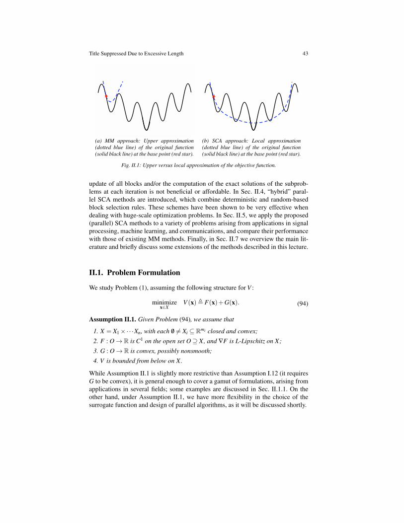
Title Suppressed Due to Excessive Length 43
(a) MM approach: Upper approximation(dotted blue line) of the original function(solid black line) at the base point (red star).
(b) SCA approach: Local approximation(dotted blue line) of the original function(solid black line) at the base point (red star).
Fig. II.1: Upper versus local approximation of the objective function.
update of all blocks and/or the computation of the exact solutions of the subprob-lems at each iteration is not beneficial or affordable. In Sec. II.4, “hybrid” paral-lel SCA methods are introduced, which combine deterministic and random-basedblock selection rules. These schemes have been shown to be very effective whendealing with huge-scale optimization problems. In Sec. II.5, we apply the proposed(parallel) SCA methods to a variety of problems arising from applications in signalprocessing, machine learning, and communications, and compare their performancewith those of existing MM methods. Finally, in Sec. II.7 we overview the main lit-erature and briefly discuss some extensions of the methods described in this lecture.
II.1. Problem Formulation
We study Problem (1), assuming the following structure for V :
minimizex∈X
V (x), F(x)+G(x). (94)
Assumption II.1. Given Problem (94), we assume that
1. X = X1×·· ·Xn, with each /0 6= Xi ⊆ Rmi closed and convex;
2. F : O→ R is C1 on the open set O⊇ X, and ∇F is L-Lipschitz on X;
3. G : O→ R is convex, possibly nonsmooth;
4. V is bounded from below on X.
While Assumption II.1 is slightly more restrictive than Assumption I.12 (it requiresG to be convex), it is general enough to cover a gamut of formulations, arising fromapplications in several fields; some examples are discussed in Sec. II.1.1. On theother hand, under Assumption II.1, we have more flexibility in the choice of thesurrogate function and design of parallel algorithms, as it will be discussed shortly.

44 Gesualdo Scutari and Ying Sun
II.1.1 Some motivating applications
Many problems in fields as diverse as sensor networks, imaging, machine learning,data analysis, genomics, and geophysics, can be formulated as Problem (94) and sat-isfy Assumption II.1. Some illustrative examples are documented next; see Sec. II.5for more details and some numerical results.Example #1−LASSO: Consider a linear regression model with q predictor/feature-response pairs (zi,ai)q
i=1, where ai ∈ Rm is a m-dimensional vector of features orpredictors, and zi is the associated response variable. Let z = (z1, . . . ,zq)
T denotethe q-dimensional vector of response, and A ∈Rq×m be the matrix with ai in its i-throw. Then, the LASSO problem in the so-called Lagrangian form [235], aiming atfinding a sparse vector of regression weights x∈Rm, is an instance of Problem (94),with F(x) = ‖z−Ax‖2 and G(x) = λ‖x‖1, where λ is a positive given constant.Example #2−Group LASSO: There are many regression problems wherein thecovariates within a group become nonzero (or zero) simultaneously. In such set-tings, it is natural to select or omit all the coefficient within a group together. Thegroup LASSO promotes this structure by using sums of (un-squared) `2 penalties.Specifically, consider the regression vector x ∈Rm possessing the group sparse pat-tern x = [xT
1 , . . . ,xTn ]
T , i.e., all the elements of xi either take large values or closeto zero [262]. A widely used group LASSO formulation is the instance of Prob-lem (94), with F(x) = ‖z−Ax‖2 and G(x) = λ ∑
ni=1 ‖xi‖2, and λ > 0.
Example #3−Sparse logistic regression: Logistic regression has been popular inbiomedical research for half a century, and has recently gained popularity to modela wider range of data. Given the training set zi,wiq
i=1, where zi ∈ Rm is the fea-ture vector and wi ∈ −1,1 is the label of the i-th sample, the logistic regressionproblem based on a linear logistic model consists in minimizing the negative loglikelihood [160, 213] F(x) = (1/q) ·∑q
i=1 log(1+ e−wi·zTi x); regularizations can be
introduced, e.g., in the form G(x) = λ‖x‖1 (or G(x) = λ ∑ni=1 ‖xi‖2), with λ > 0.
Clearly, this is an instance of Problem (94).Example #4−Dictionary learning: Dictionary learning is an unsupervised learningproblem that consists in finding a basis D ∈ Rq×m–called dictionary–whereby datazi ∈ Rq can be sparsely represented by coefficients xi ∈ Rm. Let Z ∈ Rq×I and Z ∈Rm×I be the data and representation matrix whose columns are the data vectors ziand coefficients xi, respectively. The DL problem is the instance of Problem (94),with F(D,X) = ‖Z−DX‖2
F and G(X) = λ‖X‖1, X = (D,X) ∈ Rq×m×Rm×I :‖Dei‖2 ≤ αi,∀i = 1, . . . ,m, where ei is the i-th canonical vector, and ‖X‖F and‖X‖1 denote the Frobenius norm and the `1 matrix norm of X, respectively. Notethat this is an example of F(D,X) that is not jointly convex in (D,X), but bi-convex(i.e., convex in D and X separately).Example #5−(Sparse) empirical risk minimization: Given a training set DiI
i=1,the parametric empirical risk minimization problem aims at finding the model h :Rm 3X→Rq, parameterized by x, that minimizes the risk function ∑
Ii=1 `(h(x;Di)),
where ` : Rq → R is a loss function, measuring the mismatch between the modeland the data. This optimization problem is a special case of Problem (94), with
Title Suppressed Due to Excessive Length 45
F(x) = ∑Ii=1 fi(x) and fi(x), `
(h(x;Di)
). To promote sparsity, one can add in the
objective function a regularizer G using, e.g., any of the surrogates of the `0 cardi-nality function listed in Table I.1 (cf. Sec. I.4.1). By absorbing the smooth G− partin F , the resulting regularized empirical risk minimization problem is still writtenin the form (94). Note that this general problem contains the previous examples asspecial cases, and generalizes them by incorporating also nonconvex regularizers.
All the above examples contain separable G. Some applications involving non-separable G are discussed next.Example #6−Robust linear regression: Linear least-squares estimates can be-have badly when the error distribution is not normal, particularly when the errorsare heavy-tailed. One remedy is to remove influential observations from the least-squares fit. Another approach, termed robust regression, is to use a fitting criterionthat is not as vulnerable as least squares to unusual (outliers) data. Consider the sys-tem model as in Example #1; a simple example of robustification is replacing the `2norm loss function with the `1 norm, which leads to the instance of Problem (94),with F(x) = 0 and G(x) = ‖Ax−v‖1 [96].Example #7−The Fermat-Weber problem: This problem consists in finding x ∈Rn such that the weighted sum of distances between x and the I anchors v1,v2, . . . ,vI is minimized [74]. It can be formulated as Problem (94), with F(x) = 0 andG(x) = ∑
Ii=1 ωi‖Aix− vi‖2, X = Rn, where Ai ∈ Rq×n, vi ∈ Rq, and ωi > 0 are
given constants, for all i.Example #8−The Total Variation (TV) image reconstruction: TV minimizingmodels have become a successful methodology for image processing, including de-noising, deconvolution, and restoration, to name a few [40]. The noise-free dis-crete TV reconstruction problem can be formulated as Problem (94) with F(X) =‖Z−AX‖2 and G(X) = λ · TV(X), X ≡ Rm×m, where A ∈ Rq×m, X ∈ Rm×m,Z ∈ Rq×m, and TV(X) , ∑
mi, j=1 ‖∇i j(X)‖p is the discrete total variational semi-
norm of X, with p = 1 or 2 and ∇i j(X) being the discrete gradient of X defined as∇i j(X), [(∇
(1)i j (X)),(∇
(2)i j (X))], with
∇(1)i j (X),
Xi+1, j−Xi, j, if i < m,
0, i = m;∇(2)i j (X)(2) ,
Xi, j+1−Xi, j, if j < m,
0, j = m;
for all i, j = 1, . . . ,m.
II.2. Parallel SCA: Vanilla VersionWe begin introducing a vanilla version of the parallel SCA framework wherein allthe block variables are updated in parallel; generalizations of this scheme will beconsidered in Sec. II.3.
The most natural parallel (Jacobi-type) solution method one can employ is solv-ing (94) blockwise and in parallel: given xk, all the (block) variables xi are updatedsimultaneously by solving the following subproblems
46 Gesualdo Scutari and Ying Sun
xk+1i ∈ argmin
xi∈Xi
F(xi,xk
−i)+G(xi,xk−i), ∀i ∈ N , 1, . . . ,n. (95)
Unfortunately, this method converges only under very restrictive conditions [16]that are seldom verified in practice (even in the absence of the nonsmooth functionG). Furthermore, the exact computation of xk+1
i is in general difficult, due to thenonconvexity of F . To cope with these two issues, the proposed approach consistsin solving for each block instead
xi(xk), argminxi∈Xi
Fi(xi |xk)+G(xi,xk−i), (96)
and then settingxk+1
i = xki + γ
k(
xi(xk)−xki
). (97)
In (96), Fi(•|xk
)represents a strongly convex surrogate replacing F(•,xk
−i), and in(97) a step-size γk ∈ (0,1] is introduced to control the “length” of the update alongthe direction xi(xk)− xk
i . The step-size is needed if one does not require that thesurrogate Fi
(•|xk
)is a global upper bound of F(•,xk
−i) (as in the MM algorithm).The surrogate function Fi has the following properties (∇Fi denotes the partial
gradient of Fi with respect to the first argument).
Assumption II.2. Each function Fi : Oi×O→ R satisfies the following conditions:
1. Fi (•|y) is τi-strongly convex on Xi, for all y ∈ X;
2. Fi (•|y) is differentiable on Oi and ∇yiF (y) = ∇Fi (yi |y), for all y ∈ X.
Stronger convergence results can be obtained under the following additional as-sumptions.
Assumption II.3. ∇Fi (xi |•) is Li-Lipschitz on X, for all xi ∈ Xi.
Assumption II.3∗. Fi (•|•) is continuous on Oi×O.
Assumption II.2 states that Fi should be regarded as a (simple) convex approxi-mation of F at the current iterate xk that preserves the first order properties of F .Note that, as anticipated, Fi need not be a global upper bound of F(•,x−i). Further-more, the above assumptions guarantee that the mapping x(x) , (xi(x))n
i=1, withxi : X → Xi defined in (96), enjoys the following properties that are instrumental toprove convergence of the algorithm to stationary solutions of Problem (94).
Lemma II.4 (Continuity of x ). Consider Problem (94) under Assumption II.1. Thefollowing hold:
(a) If Assumptions II.2 and II.3∗are satisfied, x(•) is continuous on X;
(b) If Assumptions II.2 and II.3 are satisfied, and G is separable, x(•) is Lipschitzcontinuous on X.
Proof. See Appendix–Sec. II.6.1.
Title Suppressed Due to Excessive Length 47
Other properties of the best-response (e.g., in the presence of nonconvex constraints)can be found in [77, 207].
The described algorithm is based on solving in parallel the subproblems in (96),converging thus to fixed-points of the mapping x(•). It is then natural to ask whichrelation exists between these fixed points and the (d-)stationary solutions of Prob-lem (94). The following lemma addresses this question.
Lemma II.5 (On the fixed-points of x). Given Problem (94) under Assumption II.1,let each Fi in (96) be chosen according to Assumption II.2. The following hold.
(a) The set of fixed-points of x(•) coincides with that of the coordinate-wise d-stationary solutions of (94);
(b) If, in addition, G is separable–G(x) = ∑ni=1 gi (xi)–then the set of fixed-points
coincides with that of d-stationary solutions of (94).
Proof. The proof of statement (b) can be found in [79, Proposition 8]. The proof ofstatement (a) follows similar steps and thus is omitted.
To complete the description of the algorithm, we need to specify how to choosethe step-size γk ∈ (0,1] in (97). Any of the following standard rules can be used.
Assumption II.6. The step-size sequence γk ∈ (0,1]k∈N+ satisfies any of the fol-lowing rules:
1. Bounded step-size: 0 < liminfk→∞ γk ≤ limsupk→∞ γk < 2cτ/L, where cτ ,mini=1,...,n τi (cf. Assumption II.2.1);
2. Diminishing step-size: ∑∞k=0 γk =+∞ and ∑
∞k=0(γk)2
<+∞;
3. Line search: let α,δ ∈ (0,1), choose γk = δ tk , where tk is the smallest nonneg-ative integer such that
V(
xk + γk
∆ xk)
≤V (xk)+α · γk
(∇F(xk)T
∆ xk +n
∑i=1
(G(xi(xk),xk
−i)−G
(xk))) (98)
with ∆ xk , x(xk)−xk.
The parallel SCA procedure is summarized in Algorithm 5.
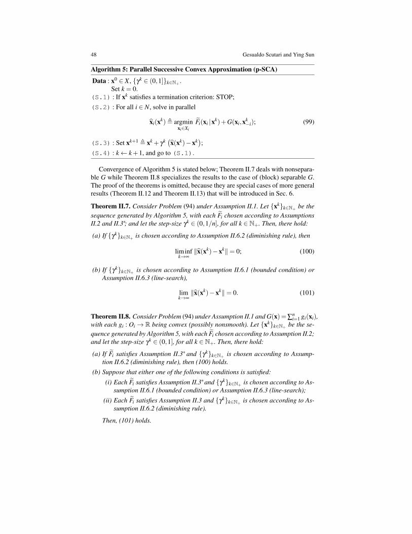
48 Gesualdo Scutari and Ying Sun
Algorithm 5: Parallel Successive Convex Approximation (p-SCA)
Data : x0 ∈ X , γk ∈ (0,1]k∈N+ .Set k = 0.
(S.1) : If xk satisfies a termination criterion: STOP;(S.2) : For all i ∈ N, solve in parallel
xi(xk), argminxi∈Xi
Fi(xi |xk)+G(xi,xk−i); (99)
(S.3) : Set xk+1 , xk + γk(x(xk)−xk
);
(S.4) : k← k+1, and go to (S.1).
Convergence of Algorithm 5 is stated below; Theorem II.7 deals with nonsepara-ble G while Theorem II.8 specializes the results to the case of (block) separable G.The proof of the theorems is omitted, because they are special cases of more generalresults (Theorem II.12 and Theorem II.13) that will be introduced in Sec. 6.
Theorem II.7. Consider Problem (94) under Assumption II.1. Let xkk∈N+ be thesequence generated by Algorithm 5, with each Fi chosen according to AssumptionsII.2 and II.3∗; and let the step-size γk ∈ (0,1/n], for all k ∈ N+. Then, there hold:
(a) If γkk∈N+ is chosen according to Assumption II.6.2 (diminishing rule), then
liminfk→∞
‖x(xk)−xk‖= 0; (100)
(b) If γkk∈N+ is chosen according to Assumption II.6.1 (bounded condition) orAssumption II.6.3 (line-search),
limk→∞‖x(xk)−xk‖= 0. (101)
Theorem II.8. Consider Problem (94) under Assumption II.1 and G(x)=∑ni=1 gi(xi),
with each gi : Oi→ R being convex (possibly nonsmooth). Let xkk∈N+ be the se-quence generated by Algorithm 5, with each Fi chosen according to Assumption II.2;and let the step-size γk ∈ (0,1], for all k ∈ N+. Then, there hold:
(a) If Fi satisfies Assumption II.3∗ and γkk∈N+ is chosen according to Assump-tion II.6.2 (diminishing rule), then (100) holds.
(b) Suppose that either one of the following conditions is satisfied:
(i) Each Fi satisfies Assumption II.3∗and γkk∈N+ is chosen according to As-sumption II.6.1 (bounded condition) or Assumption II.6.3 (line-search);
(ii) Each Fi satisfies Assumption II.3 and γkk∈N+ is chosen according to As-sumption II.6.2 (diminishing rule).
Then, (101) holds.

Title Suppressed Due to Excessive Length 49
The above theorems establish the following connection between the limit pointsof the sequence xkk∈N+ and the stationary points of Problem (94). By (101)and the continuity of x(•) (cf. Lemma II.4), we infer that every limit point x∞
of xkk∈N+ (if exists) is a fixed point of x(•) and thus, by Lemma II.5, it is acoordinate-wise d-stationary solution of Problem (94). If, in addition, G is separa-ble, x∞ is a d-stationary solution of (94). When (100) holds instead, there exists asubsequence xktt∈N+ of xkk∈N+ such that limt→∞ ‖x(xkt )− xkt‖ = 0, and theaforementioned connection with the (coordinate-wise) stationary solutions of (94)holds for every limit point of such a subsequence. The existence of a limit point ofxkk∈N+ is guaranteed under standard extra conditions on the feasible set X–e.g.,boundedness–or on the objective function V –e.g., coercivity on X .
II.2.1 Discussion on Algorithm 5
Algorithm 5 represents a gamut of parallel solution methods, each of them corre-sponding to a specific choice of the surrogate functions Fi and step-size rule. The-orems above provide a unified set of conditions for the convergence of all suchschemes. Some representative choices for Fi and γk are discussed next.On the choice of the surrogate Fi. Some examples of surrogate functions satisfyingAssumption II.2 for specific F are the following.1) Block-wise convexity. Suppose F(x1, . . . ,xn) is convex in each block xi separately(but not necessarily jointly). A natural approximation for such an F exploring its“partial” convexity is: given y = (yi)
ni=1 ∈ X ,
F(x |y) =n
∑i=1
Fi(xi |y), (102)
with each Fi(xi |y) defined as
Fi(xi |y), F(xi,y−i)+τi
2(xi−yi)
T Hi (xi−yi), (103)
where τi is any positive constant, and Hi is any mi×mi positive definite matrix (ofcourse, one can always choose Hi = I). The quadratic term in (103) can be set tozero if F(•,y−i) is strongly convex on Xi, for all y−i ∈ X−i , X1 × ·· · × Xi−1 ×Xi+1×·· ·×Xn.2) (Proximal) gradient-like approximations. If no convexity is present in F , mimick-ing proximal-gradient methods, a valid choice of F is the first order approximationof F (plus a quadratic regularization), that is, F is given by (102), with each
Fi(xi |y), ∇xiF(y)T (xi−yi)+τi
2‖xi−yi‖2. (104)
Note that the above approximation has the same form of the one used in the MMalgorithm [cf. (28)], with the difference that in (104) τi can be any positive number(and not necessarily larger than Li). When τi < Li, Fi in (104) is no longer a global

50 Gesualdo Scutari and Ying Sun
upper bound of F(•,x−i). In such cases, differently from the MM algorithm, step-size γk = 1 in Algorithm 5 may not be used at each k.3) Sum-utility function. Suppose that F(x) , ∑
Ii=1 fi(x1, . . . , xn). This structure
arises, e.g., in multi-agent systems wherein fi is the cost function of agent i thatcontrols its own block variables xi ∈ Xi. In many application it is common that thecost functions fi are convex in some agents’ variables (cf. Sec. II.5). To exploit thispartial convexity, let us introduce the following set
Ci ,
j : f j(•,x−i) is convex, ∀x−i ∈ X−i, (105)
which represents the set of indices of all the functions f j that are convex in xi, forany feasible x−i; and let Ci ⊆ Ci be any subset of Ci. Then, the following surrogatefunction satisfies Assumption II.2 while exploiting the partial convexity of F (ifany): given y = (yi)
ni=1 ∈ X ,
F(x |y) =n
∑i=1
FCi(xi |y),
with each FCi defined as
FCi(xi |y), ∑j∈Ci
f j(xi,y−i)+ ∑`/∈Ci
∇xi f`(y)T (xi−yi)
+τi
2(xi−yi)
T Hi (xi−yi),
(106)
where Hi is any mi×mi positive definite matrix. Roughly speaking, for each agenti, the above approximation function preserves the convex part of F w.r.t. xi while itlinearizes the nonconvex part.4) Product of functions. Consider an F that is written as the product of functions(see [208] for some examples); without loss of generality, here we study only thecase of product of two functions. Let F(x) = f1(x) f2(x), with f1 and f2 convexand non-negative on X ; if the functions are just block-wise convex, the proposedapproach can be readily extended. In view of the expression of the gradient of Fand Assumption II.2.2, ∇xF = f2∇x f1 + f1∇x f2, it seems natural to consider thefollowing approximation: given y ∈ X ,
F(x |y) = f1(x) f2(y)+ f1(y) f2(x)+τi
2(x−y)T H(x−y),
where, as usual, H is a positive definite matrix; this term can be omitted if f1 andf2 are positive on the feasible set and f1 + f2 is strongly convex (for example if oneof the two functions is strongly convex). In case f1 and f2 are still positive but notnecessarily convex, we can use the expression
F(x |y) = f1(x |y) f2(y)+ f1(y) f2(x |y),
Title Suppressed Due to Excessive Length 51
where f1 and f2 are any legitimate surrogates of f1 and f2, respectively. Finally,if f1 and f2 can take nonpositive values, introducing h1(x |y) , f1(x |y) f2(y) andh2(x |y), f1(y) f2(x |y), one can write
F(x |y) = h1(x |y)+ h2(x |y),
where h1 (resp. f1) and h2 (resp. f2) are legitimate surrogates of h1 (resp. f1) and h2(resp. f2), respectively. Note that in this last case, we no longer need the quadraticterm because it is already included in the approximations f1 and f2, and h1 and h2,respectively. As the final remark, note that the functions F discussed above belongto a class of nonconvex functions for which it does not seem possible to find a globalconvex upper bound; therefore, the MM techniques introduced in Lecture I are notreadily applicable.5) Composition of functions. Let F(x) = h(f(x)), where h : Rq→ R is a finite con-vex smooth function such that h(u1, . . . ,uq) is nondecreasing in each component,and f : Rm → Rq is a smooth mapping, with f(x) = ( f1(x), . . . , fq(x))T and fi notnecessarily convex. Examples of functions F belonging to such a class are thosearising from nonlinear least square-based problems, that is, F(x) = ‖f(x)‖2, wheref(x) is a smooth nonlinear (possibly) nonconvex map. A convex approximation sat-isfying Assumption II.2 is: given y ∈ Rm,
F(x |y), h(f(y)+∇f(y)(x−y))+τ
2‖x−y‖2, (107)
where ∇f(y) denotes the Jacobian of f at y.
On the choice of the step-size γk. Some possible choices for the step-size satisfyingAssumption II.6 are the following.1) Bounded step-size: Assumption II.6.1 requires the step-size to be eventually in theinterval [δ ,2cτ/L), for some δ > 0. A simple choice is γk = γ > 0, with 2cτ/γ > Land for all k. This simple (but conservative) condition imposes a constraint only onthe ratio cτ/γ , leaving free the choice of one of the two parameters. An interest-ing case is when the proximal gradient-like approximation in (104) is used. Settingtherein each τi > L/2 allows one to use step-size γ = 1, obtaining thus the MMalgorithm as a special case.2) Diminishing step-size: In scenarios where the knowledge of system parameters,e.g., L, is not available, one can use a diminishing step-size satisfying Assump-tion II.6.2. Two examples of diminishing step-size rules are:
γk = γk−1(
1− ε γk−1), k = 1, . . . , γ
0 < 1/ε; (108)
γk =γk−1 +α(k)
1+β (k), k = 1, . . . , γ
0 = 1; (109)
where in (108) ε ∈ (0,1) is a given constant, whereas in (109) α(k) and β (k) aretwo nonnegative real functions of k ≥ 1 such that: i) 0 ≤ α(k) ≤ β (k); and ii)
52 Gesualdo Scutari and Ying Sun
α(k)/β (k)→ 0 as k→ ∞ while ∑k (α(k)/β (k)) = ∞. Examples of such α(k) andβ (k) are: α(k) = α or α(k) = log(k)α , and β (k) = β · k or β (k) = β ·
√k, where
α,β are given constants satisfying α ∈ (0,1), β ∈ (0,1), and α ≤ β .3) Line search: Assumption II.6.3 is an Armijo-like line-search that employs a back-tracking procedure to find the largest γk generating sufficient descent of the objectivefunction at xk along the direction ∆ x(xk). Of course, using a step-size generated byline-search will likely be more efficient in terms of iterations than the one based ondiminishing step-size rules. However, as a trade-off, performing line-search requiresevaluating the objective function multiple times per iteration; resulting thus in morecostly iterations. Furthermore, performing a line-search on a multicore architecturerequires some shared memory and coordination among the cores/processors.
II.3. Parallel SCA: Selective updatesThe parallel SCA algorithm introduced in Sec. II.2 consists in updating at each it-eration all the block variables by computing the solutions of subproblems in theform (96). In this section, we generalize the algorithm by i) unlocking parallel up-dates of a subset of all the blocks at a time, and ii) allowing inexact computations ofthe solution of each subproblem. This is motivated by applications where computingthe exact solutions of large-scale subproblems is computationally demanding and/orupdating all the block variables at each iteration is not beneficial; see Sec. II.5 forsome examples.Inexact solutions: Subproblems in (96) are solved inexactly by computing zk satis-fying ‖zk
i − xi(xk)‖ ≤ εki , where εk
i is the desired accuracy (to be properly chosen).Some conditions on the inexact solution (and thus associated error) are needed toguarantee convergence on the resulting algorithm, as stated next.
Assumption II.9. Given xi(xk) as defined in (96), the inexact solutions zki satisfies:
for all i = 1, . . . ,n,
1. ‖zki − xi
(xk)‖ ≤ εk
i and limk→∞ εki = 0;
2. Fi(zk
i |xk)+G
(zk
i ,xk−i)≤ Fi
(xk
i |xk)+G
(xk).
The above conditions are quite natural: Assumption II.9.1 states that the errormust asymptotically vanish [subproblems (96) need to be solved with increasingaccuracy] while Assumption II.9.2 requires that zk
i generates a decrease in the ob-jective function of subproblem (96) at iteration k [zk
i need not be a minimizer of(96)].Updating only some blocks: At each iteration k a suitable chosen subset of blocks–say Sk ⊆ N [recall that N , 1, . . . ,n]–is selected and updated by computing foreach block i ∈ Sk an inexact solution zk
i of the associated subproblem (96): given xk
and Sk, let
xk+1i =
xk
i + γk (zki −xk
i ), if i ∈ Sk,
xki if i /∈ Sk.
Title Suppressed Due to Excessive Length 53
Several options are possible for the block selection rule Sk. For instance, one canchoose the blocks to update according to some deterministic (cyclic) or random-based rule. Greedy-like schemes–updating at each iteration only the blocks that are“far away” from the optimum–have been shown to be quite effective in some ap-plications. Finally, one can also adopt hybrid rules that properly combine the afore-mentioned selection methods. For instance, one can first select a subset of blocksuniformly at random, and then within such a pool updating only the blocks resultingfrom a greedy rule. Of course some minimal conditions on the updating rule arenecessary to guarantee convergence, as stated below.
Assumption II.10. The block selection satisfies one of the following rules:
1. Essentially cyclic rule: Sk is selected so that⋃T−1
s=0 Sk+s = N, for all k ∈N+ andsome finite T > 0;
2. Greedy rule: Each Sk contains at least one index i such that
Ei(xk)≥ ρ max
j∈NE j(xk),
where ρ ∈ (0,1] and Ei(xk)
is an error bound function satisfying
si · ‖xi(xk)−xki ‖ ≤ Ei(xk)≤ si · ‖xi(xk)−xk
i ‖, (110)
for some 0 < si ≤ si <+∞;
3. Random-based rule: The sets Sk are realizations of independent random sets SSSk
taking value in the power set of N, such that P(i ∈ SSSk) ≥ p, for all i = 1, . . . ,nand k ∈ N+, and some p > 0.
The above selection rules are quite general and have a natural interpretation. Thecyclic rule [Assumption II.10.1] requires that all the blocks are updated (at least)once within T consecutive iterations, where T is an arbitrary (finite) integer. As-sumption II.10.2 is a greedy-based rule: only the blocks that are “far” from the opti-mum need to be updated at each iteration; Ei
(xk)
can be viewed as a local measureof the distance of block i from optimality. The greedy rule in Assumption II.10.2thus calls for the updates of one block that is within a fraction ρ from the largestdistance Ei
(xk). Some examples of valid error bound functions Ei are discussed in
Sec. II.3.1. Finally, Assumption II.10.3 is a random selection rule: blocks can beselected according to any probability distribution as long as they have a positiveprobability to be picked. Specific rules satisfying Assumption II.10 are discussed inSec. II.3.1.
The described parallel selective SCA method is summarized in Algorithm 6, andtermed “inexact FLEXible parallel sca Algorithm” (FLEXA).

54 Gesualdo Scutari and Ying Sun
Algorithm 6: Inexact Flexible Parallel SCA Algorithm (FLEXA)
Data : x0 ∈ X , γk ∈ (0,1]k∈N+ , εki ≥ 0, for all i ∈ N and k ∈ N+, ρ ∈ (0,1].
Set k = 0.(S.1) : If xk satisfies a termination criterion: STOP;(S.2) : Choose a set Sk according to any of the rules in Assumption II.10;(S.3) : For all i ∈ Sk, solve (96) with accuracy εk
i :find zk
i ∈ Xi s.t. ‖zki − xi
(xk)‖ ≤ εk
i ;
Set zki = zk
i for i ∈ Sk, and zki = xk
i for i 6∈ Sk;
(S.4) : Set xk+1 , xk + γk (zk−xk);(S.5) : k← k+1, and go to (S.1).
To complete the description of the algorithm, we need to specify how to choosethe step-size γk in Step 4. Assumption II.11 below provides some standard rules.
Assumption II.11. The step-size sequence γk ∈ (0,1]k∈N+ satisfies any of the fol-lowing rules:
1. Bounded step-size: 0 < liminfk→∞ γk ≤ limsupk→∞ γk < cτ/L, where cτ ,mini=1,...n τi;
2. Diminishing step-size: ∑∞k=0 γk = +∞ and ∑
∞k=0(γ
k)2 < +∞. In addition, if Sk
is chosen according to the cyclic rule [Assumption II.10.1], γk further satisfies0 < η1 ≤ γk+1/γk ≤ η2 <+∞, for sufficiently large k, and some η1 ∈ (0,1) andη2 ≥ 1;
3. Line-search: Let α,δ ∈ (0,1), choose γk = δ tk , where tk is the smallest non-negative integer such that
V (xk + γk
∆ xk)≤
V (xk)+α · γk
(∇F(xk)T
∆ xk + ∑i∈Sk
(G(zk
i ,xk−i)−G(xk)
)), (111)
where ∆ xk , (zk−xk).
Convergence of Algorithm 6 is stated below and summarized in the flow chart inFig. II.2. Theorem II.12 applies to settings where the step-size is chosen accordingto the bounded rule or line-search while Theorem II.13 states convergence under thediminishing step-size rule.
Theorem II.12. Consider Problem (94) under Assumption II.1. Let xkk∈N+ be thesequence generated by Algorithm 6, under the following conditions:
(i) Each surrogate function Fi satisfies Assumptions II.2-II.3 or II.2-II.3∗;
(ii) Sk is chosen according to any of the rules in Assumption II.10;
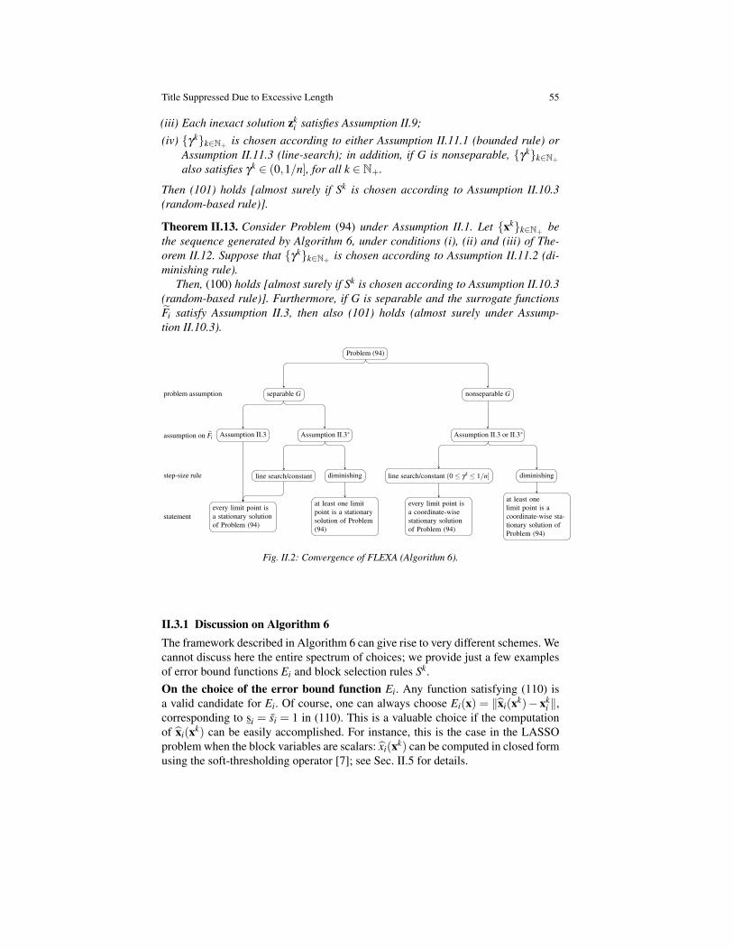
Title Suppressed Due to Excessive Length 55
(iii) Each inexact solution zki satisfies Assumption II.9;
(iv) γkk∈N+ is chosen according to either Assumption II.11.1 (bounded rule) orAssumption II.11.3 (line-search); in addition, if G is nonseparable, γkk∈N+
also satisfies γk ∈ (0,1/n], for all k ∈ N+.
Then (101) holds [almost surely if Sk is chosen according to Assumption II.10.3(random-based rule)].
Theorem II.13. Consider Problem (94) under Assumption II.1. Let xkk∈N+ bethe sequence generated by Algorithm 6, under conditions (i), (ii) and (iii) of The-orem II.12. Suppose that γkk∈N+ is chosen according to Assumption II.11.2 (di-minishing rule).
Then, (100) holds [almost surely if Sk is chosen according to Assumption II.10.3(random-based rule)]. Furthermore, if G is separable and the surrogate functionsFi satisfy Assumption II.3, then also (101) holds (almost surely under Assump-tion II.10.3).
Problem (94)
separable G nonseparable G
Assumption II.3 Assumption II.3∗ Assumption II.3 or II.3∗
line search/constant diminishing line search/constant (0≤ γk ≤ 1/n] diminishing
every limit point isa stationary solutionof Problem (94)
at least one limitpoint is a stationarysolution of Problem(94)
every limit point isa coordinate-wisestationary solutionof Problem (94)
at least onelimit point is acoordinate-wise sta-tionary solution ofProblem (94)
problem assumption
assumption on Fi
step-size rule
statement
Fig. II.2: Convergence of FLEXA (Algorithm 6).
II.3.1 Discussion on Algorithm 6The framework described in Algorithm 6 can give rise to very different schemes. Wecannot discuss here the entire spectrum of choices; we provide just a few examplesof error bound functions Ei and block selection rules Sk.On the choice of the error bound function Ei. Any function satisfying (110) isa valid candidate for Ei. Of course, one can always choose Ei(x) = ‖xi(xk)− xk
i ‖,corresponding to si = si = 1 in (110). This is a valuable choice if the computationof xi(xk) can be easily accomplished. For instance, this is the case in the LASSOproblem when the block variables are scalars: xi(xk) can be computed in closed formusing the soft-thresholding operator [7]; see Sec. II.5 for details.
56 Gesualdo Scutari and Ying Sun
In situations where the computation of ‖xi(xk)−xki ‖ is not possible or advisable
(e.g., when a closed form expression is lacking and the blocks have a large size),one can resort to alternative less expensive metrics satisfying (110). For example,assume momentarily that G ≡ 0. Then, it is known [78, Proposition 6.3.1] that,under the stated assumptions, ‖ΠXi(xk
i −∇xiF(xk))− xki ‖ is an error bound for the
minimization problem in (96) and therefore it satisfies (110), where ΠXi(y) denotesthe Euclidean projection of y onto the closed and convex set Xi. In this case, onecan choose Ei(xk) = ‖ΠXi(xk
i −∇xiF(xk))− xki ‖. If G(x) 6≡ 0 things become more
involved. In several cases of practical interest, adequate error bounds can be derivedusing [238, Lemma 7].
It is interesting to note that the computation of Ei is only needed if a partialupdate of the (block) variables is performed; otherwise (when Sk = N) one can dis-pense with the computation of Ei.On the block selection rule Sk. The selection rules satisfying Assumption II.10are extremely flexible, ranging from deterministic to random-based selection rules.For instance, one can always choose Sk = N, resulting in the simultaneous deter-ministic update of all the (block) variables at each iteration (Algorithm 5). At theother extreme, one can update a single (block) variable per time, thus obtaining aGauss-Southwell kind of method. Virtually, one can explore all the possibilities “inbetween”, e.g., by choosing properly Sk and leveraging the parameter ρ in (110) tocontrol the desired degree of parallelism or using suitably chosen cyclic-based aswell as random-based rules. This flexibility can be coupled with the possibility ofcomputing at each iteration only inexact solutions (Step 3), without affecting theconvergence of the resulting scheme (provided that Assumption II.9 is satisfied).
The selection of the most suitable updating rule depends on the specific problem,including the problem scale, computational environment, data acquisition process,as well as the communication among the processors. For instance, versions of Al-gorithm 6 where all (or most of) the variables are updated at each iteration are par-ticularly amenable to implementation in distributed environments (e.g., multi-usercommunications systems, ad-hoc networks, etc.). In fact, in these settings, not onlythe calculation of the inexact solutions zk
i can be carried out in parallel, but the in-formation that “the i-th subproblem” has to exchange with the “other subproblems”in order to compute the next iteration is very limited. A full appreciation of the po-tentialities of this approach in distributed settings depends however on the specificapplication under consideration; we discuss some examples in Sec. II.5. The cyclicorder has the advantage of being extremely simple to implement. Random selection-based rules are essentially as cheap as cyclic selections while alleviating some of thepitfalls of cyclic updates. They are also relevant in distributed environments whereindata are not available in their entirety, but are acquired either in batches or over anetwork. In such scenarios, one might be interested in running the optimization at acertain instant even with the limited, randomly available information. A main lim-itation of random/cyclic selection rules is that they remain disconnected from thestatus of the optimization process, which instead is exactly the kind of behavior thatgreedy-based updates try to avoid, in favor of faster convergence, but at the cost ofmore intensive computation.
Title Suppressed Due to Excessive Length 57
We conclude the discussion on the block selection rules providing some specificdeterministic and random-based rules that we found effective in our experiments.• Deterministic selection: In addition to the selection rules discussed above, a spe-cific (albeit general) approach is to define first a finite cover SiM
i=1 of N and thenupdate the blocks by selecting the Si’s cyclically. It is also admissible to randomlyshuffle the order of the sets Si before one update cycle.• Random-based selection: The sampling rule SSS (for notational simplicity the it-eration index k will be omitted) is uniquely characterized by the probability massfunction
P(S), P(SSS = S) , S⊆ N,
which assign probabilities to the subsets S of N. Associated with SSS, define the prob-abilities q j , P(|SSS|= j), for j = 1, . . . ,n. The following proper sampling rules, pro-posed in [197] for convex problems with separable G, are instances of rules satisfy-ing Assumption II.10.3.
1. Uniform (U) sampling: All blocks are selected with the same (non zero) proba-bility:
P(i ∈ SSS) = P( j ∈ SSS) =E [|SSS|]
n, ∀i 6= j ∈ N.
2. Doubly Uniform (DU) sampling: All sets S of equal cardinality are generatedwith equal probability, i.e., P(S) = P(S′), for all S,S
′ ⊆ N such that |S| = |S′ |.The density function is then
P(S) =q|S|(n|S|
) .
3. Nonoverlapping Uniform (NU) sampling: It is a uniform sampling assigningpositive probabilities only to sets forming a partition of N. Let S1, . . . ,Sp be apartition of N, with each
∣∣Si∣∣> 0, the density function of the NU sampling is:
P(S) =
1p, if S ∈
S1, . . . ,Sp
;
0 otherwise;
which corresponds to P(i ∈ SSS) = 1/p, for all i ∈ N.4. Nice Sampling (NS): Given an integer 0 ≤ τ ≤ n, a τ-nice sampling is a DU
sampling with qτ = 1 (i.e., each subset of τ blocks is chosen with the sameprobability).Using the NS one can control the degree of parallelism of the algorithm bytuning the cardinality τ of the random sets generated at each iteration, whichmakes this rule particularly appealing in a multi-core environment. Indeed, onecan set τ equal to the number of available cores/processors, and assign eachblock coming out from the greedy selection (if implemented) to a dedicatedprocessor/core.
58 Gesualdo Scutari and Ying Sun
As a final remark, note that the DU/NU rules contain as special cases sequen-tial and fully parallel updates wherein at each iteration a single block is updateduniformly at random, or all blocks are updated.
5. Sequential sampling: It is a DU sampling with q1 = 1, or a NU sampling withp = n and S j = j, for j = 1, . . . , p.
6. Fully parallel sampling: It is a DU sampling with qn = 1, or a NU sampling withp = 1 and S1 = N.
Other interesting uniform and nonuniform practical rules (still satisfying As-sumption II.10) can be found in [196, 197]. Furthermore, see [55, 56] for extensivenumerical results comparing the different sampling schemes.
II.3.2 Convergence analysis of Algorithm 6
In this subsection, we prove convergence of Algorithm 6 (Theorems II.12 and II.13).We consider only deterministic block selection rules (namely Assumption II.10.1and Assumption II.10.2); the proof under random-based block selection rules fol-lows similar steps and thus is omitted.
PreliminariesWe first introduce some preliminary technical results that will be used to prove theaforementioned theorems.
Lemma II.14 (Descent Lemma [14]). Let F : Rm → R be continuously differen-tiable, with L-Lipschitz gradient. Then, there holds:∣∣F(y)−F(x)−∇F(x)T (y−x)
∣∣≤ L2‖y−x‖2, ∀x, y ∈ Rm. (112)
Lemma II.15. Let (ai)ni=1 be a n-tuple of nonnegative numbers such that ∑
ni=1 ai ≥
δ , with δ > 0. Then, it holds ∑ni=1 ai ≤ n
δ∑
ni=1 a2
i .
Proof. Define a , [a1, . . . ,an]T . The desired result follows readily from ‖a‖2
2
(a)≥
1n ‖a‖2
1
(b)≥ δ
n ‖a‖1, where in (a) we used the Jensen’s inequality and a ≥ 0 while (b)is due to ‖a‖1 ≥ δ .
Lemma II.16 ( [17, Lemma 1]). Let Y kk∈N+ , W kk∈N+ , and Zkk∈N+ be threesequences such that W k is nonnegative for all k. Assume that
Y k+1 ≤ Y k−W k +Zk, k = 0,1, . . . , (113)
and that the seriesT∑
k=0Zk converges as T → ∞. Then either Y k →−∞, or else Y k
converges to a finite value and∞
∑k=0
W k < ∞.

Title Suppressed Due to Excessive Length 59
Lemma II.17. Let xkk∈N+ be the sequence generated by Algorithm 6, with eachγk ∈ (0,1/n). For every k ∈ N+ and Sk ⊆ N, there holds:
G(xk+1)−G(xk)≤ γk∑
i∈Sk
(G(zk
i ,xk−i)−G(xk)
), (114)
where zki is the inexact solution defined in Step 3 of the algorithm.
Furthermore, if G is separable, we have: for γk ∈ (0,1),
G(xk+1)−G(xk)≤ γk∑
i∈Sk
(gi(zk
i )−gi(xki )). (115)
Proof. See Appendix–Sec. II.6.2.
Lemma II.18. Under Assumptions II.1, II.2, and II.9, the inexact solution zki satis-
fies∇xiF(xk)T (zk
i −xki )+G(zk
i ,xk−i)−G(xk)≤−τi
2‖zk
i −xki ‖2. (116)
Proof. The proof follows readily from the strong convexity of Fi and Assump-tion II.9.2.
Lemma II.19. Let Sk be selected according to the greedy rule (cf. Assumption II.10.2).Then, there exists a constant 0 < c≤ 1 such that∥∥∥(x(xk)−xk
)Sk
∥∥∥≥ c∥∥∥x(xk)−xk
∥∥∥ . (117)
Proof. See Appendix–Sec. II.6.3.
Proposition II.20. Let xkk∈N+ be the sequence generated by Algorithm 6, in thesetting of Theorem II.12 or Theorem II.13. The following hold [almost surely, if Sk
is chosen according to Assumption II.10.3 (random-based rule)]:
(a)∞
∑k=0
γk∥∥∥zk−xk
∥∥∥2<+∞; (118)
(b)
limk→∞‖xk+1−xk‖= 0. (119)
Proof. Without loss of generality, we consider next only the case of nonseparableG. By the descent lemma (cf. Lemma 114) and Steps 3-4 of the algorithm, we have
F(xk+1)≤ F(xk)+ γk∇F(xk)T (zk−xk)+
(γk)2 L2‖zk−xk‖2.
Consider the case of G nonseparable. We have:
V (xk+1) = F(xk+1)+G(xk+1)

60 Gesualdo Scutari and Ying Sun
(114)≤ V (xk)+ γ
k∇F(xk)T (zk−xk)+
(γk)2 L2‖zk−xk‖2
+γk∑
i∈Sk
(G(zk
i ,xk−i)−G(xk)
)(120)
(116)≤ V (xk)− γk
2(cτ − γ
kL)‖zk−xk‖2. (121)
If γk satisfies either Assumption II.11.1 (bounded rule) or Assumption II.11.2(diminishing rule), statement (a) of the proposition comes readily from Lemma II.16and Assumption II.1.4.
Consider now the case where γk is chosen according to Assumption II.11.3 (linesearch). First of all, we prove that there exists a suitable γk ∈ (0,γ0], with γ0 ∈(0,1/n] (if G is separable γ0 ∈ (0,1]), such that the Armijo-like condition (111)holds. By (120), the line-search condition (111) is satisfied if
γk
(∇F(xk)T (zk−xk)+ ∑
i∈Sk
(G(zk
i ,xk−i)−G(xk)
))+
(γk)2 L2‖zk−xk‖2
≤ α · γk
(∇F(xk)T (zk−xk)+ ∑
i∈Sk
(G(zk
i ,xk−i)−G(xk)
)),
which, rearranging the terms, yields
γk ·L2‖zk−xk‖2
≤−(1−α)
(∇F(xk)T (zk−xk)+ ∑
i∈Sk
(G(zk
i ,xk−i)−G(xk)
)). (122)
Since (cf. Lemma II.18)
‖zk−xk‖2 ≤− 2cτ
·(
∇F(xk)T (zk−xk)+ ∑i∈Sk
(G(zk
i ,xk−i)−G(xk)
)),
inequality (122) [and thus (111)] is satisfied by any γk ≤min
γ0, cτ (1−α)L
<+∞.
We show next that γk obtained by (111) is uniformly bounded away from zero.This is equivalent to show tk < +∞. Without loss of generality we consider tk ≥ 1[otherwise (111) is satisfied by γk = γ0]. Since tk is the smallest positive integer suchthat (111) holds with γk = δ tk , it must be that the same inequality is not satisfied byγk = δ tk−1. Consequently, it must be δ tk−1 > cτ (1−α)
L , and thus
γk ≥min
γ
0,cτ (1−α)
L·δ. (123)

Title Suppressed Due to Excessive Length 61
Using (123) in (121), we obtain
V (xk+1)≤V (xk)−β2 ‖zk−xk‖2, ∀k ∈ N+, (124)
where β2 > 0 is some finite constant. The rest of the proof follows the same argu-ments used to prove the statements of the proposition from (121).
We prove now statement (b). By Step 4 of Algorithm 6, it suffices to show that
limk→∞
γk ‖zk−xk‖= 0.
Using (118), we havelimk→∞
γk‖zk−xk‖2 = 0.
Since γk ∈ (0,1], it holds
limk→∞
(γ
k ‖zk−xk‖)2≤ lim
k→∞γ
k‖zk−xk‖2 = 0. (125)
This completes the proof.
Proof of Theorem II.12
We prove (101) for each of the block selection rules in Assumption II.10 separately.
• Essentially cyclic rule [Assumption II.10.1]: We start bounding ‖x(xk)−xk‖ asfollows:
‖x(xk)−xk‖
≤n
∑i=1‖xi(xk)−xk
i ‖
≤n
∑i=1
(‖xi(xk)− xi(xk+sk
i )‖+‖xi(xk+ski )−xk+sk
ii ‖+‖xk+sk
ii −xk
i ‖) (126)
where ski ,mint ∈ 1, . . . ,T| i ∈ Sk+t, so that k+ sk
i is the first time that block iis selected (updated) since iteration k. Note that 1≤ sk
i ≤ T , for all i∈N and k ∈N+
(due to Assumption II.10.1). We show next that the three terms on the RHS of (126)are asymptotically vanishing, which proves (101).
Since 1≤ ski ≤ T , we can write
limk→∞‖xk+sk
i −xk‖ ≤ limk→∞
T
∑j=1‖xk+ j−xk+ j−1‖ (119)
= 0, (127)
which, by the continuity of x(•) (cf. Lemma II.4), leads also to
62 Gesualdo Scutari and Ying Sun
limk→∞‖xi(xk)− xi(xk+sk
i )‖= 0. (128)
Let Ti ⊆ N+ be the set of iterations at which block i is updated. It follows fromAssumption II.10.1 that |Ti|=+∞, for all i ∈ N. This together with (118) implies
∑k∈Ti
‖zki −xk
i ‖2 <+∞, ∀i ∈ N,
and thus
limTi3k→∞
∥∥∥zki −xk
i
∥∥∥= 0 ⇒ limk→∞
∥∥∥∥zk+ski
i −xk+ski
i
∥∥∥∥= 0, ∀i ∈ N.
Therefore,
limk→∞
∥∥∥∥xi(xk+ski )−xk+sk
ii
∥∥∥∥≤ lim
k→∞
∥∥∥∥xi(xk+ski )− zk+sk
ii
∥∥∥∥+ limk→∞
∥∥∥∥zk+ski
i −xk+ski
i
∥∥∥∥= 0, ∀i ∈ N. (129)
Combining (126) with (127)-(129) and invoking again the continuity of x(•), weconclude that limk→∞ ‖x(xk)−xk‖= 0.• Greedy rule [Assumption II.10.2]: We have
c‖x(xk)−xk‖(117)≤ ‖(x(xk)−xk)Sk‖≤ ‖(zk−xk)Sk‖+‖(x(xk)− zk)Sk‖ (130)
A.II.9.1≤ ‖zk−xk‖+ ∑
i∈Sk
εki −→k→∞
0,
where the last implication comes from limk→∞ εki = 0, for all i ∈ N–cf. Assump-
tion II.9.1–and limk→∞ ‖zk− xk‖ = 0–due to Proposition II.20 and the fact that γk
is bounded away from zero, when the step-size is chosen according to Assump-tion II.11.1 or Assumption II.11.3 [cf. (123)]. This proves (101).
Proof of Theorem II.13
Consider now the diminishing step-size rule [Assumption II.11.2].1) Proof of (100): liminfk→∞ ‖x(xk)− xk‖ = 0. By Proposition II.20 and the step-size rule, we have liminfk→∞ ‖zk−xk‖ = 0, for all choices of Sk. We proceed con-sidering each of the block selection rules in Assumption II.10 separately.• Essentially cyclic rule [Assumption II.10.1]: For notational simplicity, let usassume that Sk is a singleton, that is, Sk = ik, where ik denotes the index of theblock selected at iteration k. The proof can be readily extended to the general case|Sk|> 1.

Title Suppressed Due to Excessive Length 63
We have
liminfk→∞
‖x(xk)−xk‖(a)≤ liminf
r→∞‖x(xrT )−xrT‖ ≤ liminf
r→∞
n
∑i=1
∥∥xi(xrT )−xrTi∥∥
≤ liminfr→∞
n
∑i=1
(∥∥∥xi(xrT+srTi )−xrT+srT
ii
∥∥∥+∥∥∥xrT+srTi
i −xrTi
∥∥∥+∥∥∥xi(xrT )− xi(xrT+srTi )∥∥∥)
= liminfr→∞
n
∑i=1
∥∥∥xi(xrT+srTi )−xrT+srT
ii
∥∥∥+ lim
r→∞
n
∑i=1
∥∥∥xrT+srTi
i −xrTi
∥∥∥︸ ︷︷ ︸(127)= 0
+ limr→∞
n
∑i=1
∥∥∥xi(xrT )− xi(xrT+srTi )∥∥∥︸ ︷︷ ︸
(128)= 0
≤ liminfr→∞
n
∑i=1
∥∥∥zrT+srTi
i −xrT+srTi
i
∥∥∥+ limr→∞
n
∑i=1
∥∥∥xi(xrT+srTi )− zrT+srT
ii
∥∥∥︸ ︷︷ ︸(A.II.9.1)≤ lim
r→∞
n
∑i=1
εrT+srT
ii
(A.II.9.1)= 0
≤ liminfr→∞
(r+1)T
∑k=rT+1
∥∥∥zkik −xk
ik
∥∥∥ , (131)
where (a) follows from the fact that the infimum of a subsequence is larger than thatof the original sequence.
To complete the proof, we show next that the term on the RHS of (131) is zero.Recalling that if the cyclic block selection rule is implemented, the diminishingstep-size γk is assumed to further satisfy η1 ≤ γk+1/γk ≤ η2, with η1 ∈ (0,1) andη2 ≥ 1 (cf. Assumption II.11.2), we have
+∞(118)≥ lim
k→∞
k
∑t=1
γt ‖zt −xt‖2 = lim
k→∞
k
∑t=1
γt ‖zt
it −xtit‖2
= limk→∞
k
∑r=0
(r+1)T
∑t=rT+1
γt ‖zt
it −xtit‖2
≥(η1)T−1 lim
k→∞
k
∑r=0
γrT+1
(r+1)T
∑t=rT+1
‖ztit −xt
it‖2,
(132)
where in the last inequality we used γk+1/γk ≥ η1. Since
+∞ = limk→∞
k
∑t=1
γt = lim
k→∞
k
∑r=0
(r+1)T
∑t=rT+1
γt ≤ T · (η2)
T−1 limk→∞
k
∑r=0
γrT+1,
it follows from (132) that
64 Gesualdo Scutari and Ying Sun
liminfr→∞
(r+1)T
∑t=rT+1
‖ztit −xt
it‖2 = 0, (133)
which, combined with (131), proves the desired result.
•Greedy rule [Assumption II.10.2]: Taking the liminf on both sides of (130) leadsto the desired result.
2) Proof of (101): limsupk→∞ ‖x(xk)− xk‖ = 0. Recall that in this setting, x(•) isLipschitz continuous with constant L. We prove the result for the essentially cyclicrule and greedy rule separately.• Essentially cyclic rule [Assumption II.10.1]: As in the proof of Theorem II.13,let us assume w.l.o.g. that Sk = ik, where ik denotes the index of the block selectedat iteration k.
By (126)-(129), it is sufficient to prove limsupk→∞ ‖zk+sk
ii − xk+sk
ii ‖ = 0, for all
i ∈ N. Since
limsupk→∞
‖zk+ski
i −xk+ski
i ‖ ≤ limsupk→∞
(k+1)T
∑t=k T+1
‖ztit −xt
it‖︸ ︷︷ ︸,∆ k
(134)
we prove next limsupk→∞ ∆ k = 0.Assume on the contrary that limsupk→∞ ∆ k > 0. Since liminfk→∞ ∆ k = 0 [cf. (133)],
there exists a δ > 0 such that ∆ k < δ for infinitely many k and also ∆ k > 2 ·T δ forinfinitely many k. Therefore, there exists a set K ⊆ N+, with |K|= ∞, such that foreach k ∈ K, one can find an integer jk > k such that
∆k ≥ 2 ·δ ·T, ∆
jk ≤ δ (135)δ < ∆
` < 2 ·δ ·T, if k < ` < jk. (136)
Define the following quantities: for any k ∈ K, let
T ki , r ∈ k T +1, . . . ,(k+1)T | ir = i and tk
i ,minT ki . (137)
Note that T ki (resp. tk
i ) is the set of (iteration) indices (resp. the smallest index)within [k T + 1,(k + 1)T ] at which the block index i is selected. Because of As-sumption II.10.1, it must be 1 ≤ |T k
i | ≤ T , for all k, where |T ki | is the number of
times block i has been selected in the iteration window [k T +1,(k+1)T ]. Then wehave
δ ·T =2 ·δ ·T −δ ·T
≤∆k−T ·∆ jk =
(k+1)T
∑r=k T+1
‖zrir −xr
ir‖−T( jk+1)T
∑r= jk·T+1
‖zrir −xr
ir‖
≤n
∑i=1
∑r∈T k
i
‖zri −xr
i‖−n
∑i=1
T ·∥∥∥∥zt
jki
i −xtjki
i
∥∥∥∥

Title Suppressed Due to Excessive Length 65
≤n
∑i=1
∑r∈T k
i
‖zri −xr
i‖−n
∑i=1|T k
i | ·∥∥∥∥zt
jki
i −xtjki
i
∥∥∥∥= n
∑i=1
∑r∈T k
i
(‖zr
i −xri‖−
∥∥∥∥ztjki
i −xtjki
i
∥∥∥∥)(a)≤
n
∑i=1
∑r∈T k
i
(∥∥∥∥xi(xr)− xi(xtjki )
∥∥∥∥+∥∥∥∥xri −xt
jki
i
∥∥∥∥)+n
∑i=1
∑r∈T k
i
(εt
jki
i + εri )︸ ︷︷ ︸
εk1
(b)≤(1+ L
) n
∑i=1
∑r∈T k
i
∥∥∥∥xr−xtjki
∥∥∥∥+ εk1
≤(1+ L
) n
∑i=1
∑r∈T k
i
tjki −1
∑s=r
γs ‖zs
is −xsis‖+ ε
k1 (138)
≤(1+ L
) n
∑i=1|T k
i | ·t
jki −1
∑r=k T+1
γr ‖zr
ir −xrir‖+ ε
k1
≤(1+ L
) n
∑i=1|T k
i | ·
jk·T∑
r=k T+1γ
r ‖zrir −xr
ir‖+t
jki −1
∑r= jk·T+1
γr ‖zr
ir −xrir‖
+ εk1
≤(1+ L
)· (n ·T )
jk·T∑
r=k T+1γ
r ‖zrir −xr
ir‖+(1+ L
)·T
tjki −1
∑r= jk·T+1
γr ‖zr
ir −xrir‖︸ ︷︷ ︸
εk2
+ εk1
≤(1+ L
)· (n ·T )
jk−1
∑s=k
(s+1)T
∑r=sT+1
γr ‖zr
ir −xrir‖+ ε
k1 + ε
k2
(c)≤(1+ L
)· (n ·T )
jk−1
∑s=k
(η2)T−1
γsT+1
(s+1)T
∑r=sT+1
‖zrir −xr
ir‖︸ ︷︷ ︸=∆ s
+ εk1 + ε
k2
(135)−(136)=
(1+ L
)· (n ·T ) · (η2)
T−1jk−1
∑s=k
γsT+1
(s+1)T
∑r=sT+1
‖zrir −xr
ir‖2
‖zrir −xr
ir‖+ ε
k1 + ε
k2
(d)≤ T
δ·(1+ L
)· (n ·T ) · (η2)
T−1jk−1
∑s=k
γsT+1
(s+1)T
∑r=sT+1
‖zrir −xr
ir‖2
︸ ︷︷ ︸εk
3
+ εk1 + ε
k2 ,
where in (a) we used the reverse triangle inequality and Assumption II.9.1; (b) isdue to the Lipschitz continuity of xi; in (c) we used γk+1/γk ≤ η2, with η2 ≥ 1; and(d) is due to Lemma II.15.
We prove now that εk1 ↓ 0, εk
2 ↓ 0, and εk3 ↓ 0. Since εk
i ↓ 0 for all i ∈ N (cf.Assumption II.9.1), it is not difficult to check that εk
1 ↓ 0. The same result for εk2
66 Gesualdo Scutari and Ying Sun
comes from the following bound:
εk2 ≤
(1+ L
)·T
( jk+1)T
∑r= jk·T+1
γr ‖zr
ir −xrir‖ ≤
(1+ L
)·T · (η2)
T−1 · γ jk·T+1 ·∆ jk
(135)≤((
1+ L)·T · (η2)
T−1 ·δ)
γjk·T+1 −→
k→∞0,
Finally, it follows from (132) that the series ∑∞s=0 γ sT+1
∑(s+1)Tr=sT+1 ‖zr
ir −xrir‖2 is con-
vergent; the Cauchy convergence criterion implies that
εk3 =
jk−1
∑s=k
γsT+1
(s+1)T
∑r=sT+1
‖zrir −xr
ir‖2 −→k→∞
0.
By the vanishing properties of εk1 , εk
2 , and εk3 , there exists a sufficiently large
k ∈ K, say k, such that
εk1 ≤
T δ
4, ε
k2 ≤
T δ
4, ε
k3 ≤
δ 2
4(1+ L
)·n ·T · (η2)T−1
, ∀k ∈ K, k ≥ k,
(139)which contradicts (138). Therefore, it must be limsupk→∞ ∆ k = 0.
• Greedy rule Assumption II.10.2: By (130), it is sufficient to prove limsupk→+∞
∆ k , ‖zk − xk‖ = 0. Assume the contrary, that is, limsupk→+∞ ∆ k > 0. Sinceliminfk→+∞ ∆ k = 0 (cf. Proposition II.20), there exists a δ > 0 such that ∆ k < δ forinfinitely many k and also ∆ k > 2 · (δ/c) for infinitely many k, where 0 < c ≤ 1 isthe constant defined in Lemma II.19. Therefore, there is a set K ⊆N+, with |K|=∞,such that for each k ∈ K, there exists an integer jk > k, such that
∆ k ≥ 2δ
c, ∆ jk ≤ δ , (140)
δ < ∆ t < 2δ
cif k < t < jk. (141)
We have
δ
c=
2δ
c− δ
c
≤∥∥∥zk−xk
∥∥∥− 1c
∥∥z jk −x jk∥∥
(a)≤ ‖(x(xk)−xk)Sk‖− 1
c‖(x(x jk)−x jk)S jk ‖+ ∑
i∈Sk
εki +
1c ∑
i∈S jk
εjk
i︸ ︷︷ ︸,εk
(117)≤ ‖x(xk)−xk‖−‖x(x jk)−x jk‖+ ε
k

Title Suppressed Due to Excessive Length 67
≤ ‖x(xk)− x(x jk)‖+‖xk−x jk‖+ εk
(b)≤ (1+ L)‖xk−x jk‖+ ε
k
≤ (1+ L)jk−1
∑t=k
γt ‖zt −xt‖+ ε
k
= (1+ L)jk−1
∑t=k
γt ‖zt −xt‖2
‖zt −xt‖ + εk
(140)−(141)<
1+ Lδ
jk−1
∑t=k
γt ‖zt −xt‖2 + ε
k, (142)
where in (a) we used the triangle inequality and Assumption II.9.1; and in (b) weused the Lipschitz continuity of x.
Since εk ↓ 0 (due to εki ↓ 0, for all i; see Assumption II.9.1) and ∑
jk−1t=k γ t ‖zt −
xt‖2 −→k→∞
0 (due to ∑∞k=0 γk
∥∥zk−xk∥∥2
< +∞; see Proposition II.20), there exists a
sufficiently large k ∈ K, say k, such that
εk ≤ δ
3 · c andjk−1
∑t=k
γt ‖zt −xt‖2 ≤ δ 2
3 · c · (1+ L), ∀k ∈ K, k ≥ k, (143)
which contradicts (142). Therefore it must be limk→∞ ‖zk−xk‖= 0.
II.4. Parallel SCA: Hybrid SchemesFLEXA (Algorithm 6) and its convergence theory cover fully parallel Jacobi aswell as Gauss-Southwell-type methods, and many of their variants. Of course, everyblock selection rule Sk has advantages and disadvantages, as discussed in Sec. II.3.1.A natural question is whether it is possible to design hybrid schemes that inherit thebest of the aforementioned plain selection schemes. In the following, we introducethree hybrid strategies that are particularly well suited to parallel optimization onmulti-core/processor architectures.
II.4.1 Random-greedy schemesIn huge-scale optimization problems, the number of variables can be so large thatcomputing the error bound functions Ei for each block i is not computationallyaffordable. To reduce the computational burden, one can think of a hybrid ran-dom/greedy block selection rule that combines random and greedy updates in thefollowing form. First, a random selection is performed−the set Sk ⊆ N is generated.Second, a greedy procedure is invoked to select within the pool Sk only the subset ofblocks, say Sk ⊆ Sk, that are “promising” according to the value of Ei(xk). Finally allthe blocks in Sk are updated in parallel. This procedure captures both the advantagesof random and greedy schemes: the random selection drops off a large proportionof the blocks allowing one to save computation while the greedy selection finds the
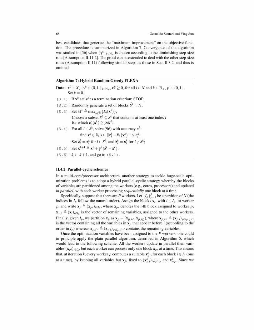
68 Gesualdo Scutari and Ying Sun
best candidates that generate the “maximum improvement” on the objective func-tion. The procedure is summarized in Algorithm 7. Convergence of the algorithmwas studied in [56] when γkk∈N+ is chosen according to the diminishing step-sizerule [Assumption II.11.2]. The proof can be extended to deal with the other step-sizerules (Assumption II.11) following similar steps as those in Sec. II.3.2, and thus isomitted.
Algorithm 7: Hybrid Random-Greedy FLEXA
Data : x0 ∈ X , γk ∈ (0,1]k∈N+ , εki ≥ 0, for all i ∈ N and k ∈ N+, ρ ∈ (0,1].
Set k = 0.(S.1) : If xk satisfies a termination criterion: STOP;(S.2) : Randomly generate a set of blocks Sk ⊆ N;(S.3) : Set Mk ,maxi∈SkEi(xk);
Choose a subset Sk ⊆ Sk that contains at least one index ifor which Ei(xk)≥ ρMk;
(S.4) : For all i ∈ Sk, solve (96) with accuracy εki :
find zki ∈ Xi s.t. ‖zk
i − xi(xk)‖ ≤ εk
i ;
Set zki = zk
i for i ∈ Sk, and zki = xk
i for i 6∈ Sk;
(S.5) : Set xk+1 , xk + γk (zk−xk);(S.6) : k← k+1, and go to (S.1).
II.4.2 Parallel-cyclic schemesIn a multi-core/processor architecture, another strategy to tackle huge-scale opti-mization problems is to adopt a hybrid parallel-cyclic strategy whereby the blocksof variables are partitioned among the workers (e.g., cores, processors) and updatedin parallel, with each worker processing sequentially one block at a time.
Specifically, suppose that there are P workers. Let IpPp=1 be a partition of N (the
indices in Ip follow the natural order). Assign the blocks xi, with i ∈ Ip, to workerp, and write xp , (xpi)i∈Ip , where xpi denotes the i-th block assigned to worker p;x−p , (xi)i/∈Ip is the vector of remaining variables, assigned to the other workers.Finally, given Ip, we partition xp as xp = (xp, i<,xp, i≥), where xp, i< , (xp j) j∈Ip, j<iis the vector containing all the variables in xp that appear before i (according to theorder in Ip) whereas xp, i≥ , (xp j) j∈Ip, j≥i contains the remaining variables.
Once the optimization variables have been assigned to the P workers, one couldin principle apply the plain parallel algorithm, described in Algorithm 5, whichwould lead to the following scheme. All the workers update in parallel their vari-ables (xpi)i∈Ip , but each worker can process only one block xpi at a time. This meansthat, at iteration k, every worker p computes a suitable zk
pi, for each block i∈ Ip (oneat a time), by keeping all variables but xpi fixed to (xk
p j)i6= j∈Ip and xk−p. Since we

Title Suppressed Due to Excessive Length 69
are solving the problems for each group of variables assigned to a worker sequen-tially but without using the most recent information for the updates, this approachseems a waste of resources. It is much more efficient to use, within each worker,a Gauss-Seidel scheme whereby the most recent iterates are used in all subsequentcalculations. More specifically, at each iteration k, each worker p computes sequen-tially an inexact version zk
pi of the solution xpi
(xk+1
p, i<,xkp, i≥,xk
−p
), with i ∈ Ip, and
updates xpi as xk+1pi = xk
pi + γk(
zkpi−xk
pi
). The scheme is summarized in Algo-
rithm 8. Convergence of the algorithm was studied in [79] when γkk∈N+ is chosenaccording to the diminishing step-size rule [Assumption II.11.2]. The proof can beextended to deal with the other step-size rules (Assumption II.11) following similarsteps as those in Sec. II.3.2, and thus is omitted.
Algorithm 8: Hybrid Parallel-Cyclic FLEXA
Data : x0 ∈ X , γk ∈ (0,1]k∈N+ , εkpi ≥ 0, for all i ∈ Ip, p ∈ 1, . . . ,P, and k ∈N+,
ρ ∈ (0,1].Set k = 0.
(S.1) : If xk satisfies a termination criterion: STOP;(S.2) : For all p ∈ 1, . . . ,P do (in parallel),
For all i ∈ Ip do (sequentially)a) Find zk
pi ∈ Xi s.t.∥∥∥zkpi− xpi
(xk+1
p, i<,xkp, i≥,x
k−p
)∥∥∥≤ εkpi;
b) Set xk+1pi , xk
pi + γk(
zkpi−xk
pi
);
(S.3) : k← k+1, and go to (S.1).
II.4.3 Parallel-Greedy-cyclic schemesIn Algorithm 8, at each iteration k, the workers update all their blocks, sequen-tially over (xpi)i∈Ip . However, in some large-scale instances of Problem (94), up-dating all variables might not always be beneficial or doable. Furthermore, usingthe latest information in the updates of each worker may require extra calculations(e.g., computing all block gradients) and communication overhead (these aspectsare discussed on specific examples in Sec. II.5). It may be of interest then to con-sider a hybrid parallel-greedy-cyclic scheme, where Algorithm 8 is equipped witha greedy selection rule. More specifically, at each iteration k, each worker proceedsas in Algorithm 8 but performing the cyclic sweeping only on a subset Sk
p of itsown variables Ip, where the subset Sk
p is chosen according to the greedy rule inAssumption II.10. To introduce formally the scheme, we extend the notation usedin Algorithm 8 as follows. We reorder the components of xp so that the first |Sk
p|variables are those in Sk
p and the remaining variables are those in Ip \ Skp; we write
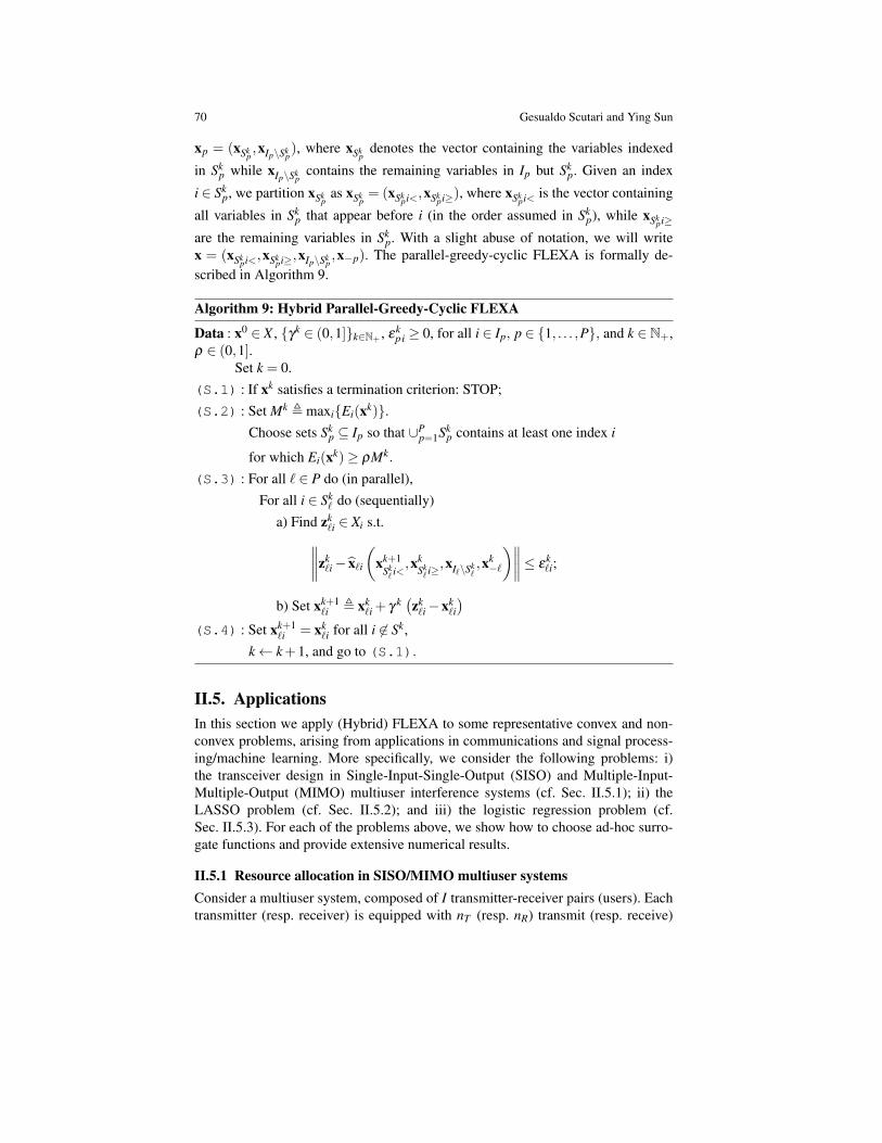
70 Gesualdo Scutari and Ying Sun
xp = (xSkp,xIp\Sk
p), where xSk
pdenotes the vector containing the variables indexed
in Skp while xIp\Sk
pcontains the remaining variables in Ip but Sk
p. Given an index
i ∈ Skp, we partition xSk
pas xSk
p= (xSk
pi<,xSkpi≥), where xSk
pi< is the vector containing
all variables in Skp that appear before i (in the order assumed in Sk
p), while xSkpi≥
are the remaining variables in Skp. With a slight abuse of notation, we will write
x = (xSkpi<,xSk
pi≥,xIp\Skp,x−p). The parallel-greedy-cyclic FLEXA is formally de-
scribed in Algorithm 9.
Algorithm 9: Hybrid Parallel-Greedy-Cyclic FLEXA
Data : x0 ∈ X , γk ∈ (0,1]k∈N+ , εkpi ≥ 0, for all i ∈ Ip, p ∈ 1, . . . ,P, and k ∈N+,
ρ ∈ (0,1].Set k = 0.
(S.1) : If xk satisfies a termination criterion: STOP;(S.2) : Set Mk ,maxiEi(xk).
Choose sets Skp ⊆ Ip so that ∪P
p=1Skp contains at least one index i
for which Ei(xk)≥ ρMk.
(S.3) : For all ` ∈ P do (in parallel),For all i ∈ Sk
` do (sequentially)a) Find zk
`i ∈ Xi s.t.∥∥∥∥zk`i− x`i
(xk+1
Sk` i<
,xkSk` i≥,xI`\Sk
`,xk−`
)∥∥∥∥≤ εk`i;
b) Set xk+1`i , xk
`i + γ k(zk`i−xk
`i
)(S.4) : Set xk+1
`i = xk`i for all i 6∈ Sk,
k← k+1, and go to (S.1).
II.5. ApplicationsIn this section we apply (Hybrid) FLEXA to some representative convex and non-convex problems, arising from applications in communications and signal process-ing/machine learning. More specifically, we consider the following problems: i)the transceiver design in Single-Input-Single-Output (SISO) and Multiple-Input-Multiple-Output (MIMO) multiuser interference systems (cf. Sec. II.5.1); ii) theLASSO problem (cf. Sec. II.5.2); and iii) the logistic regression problem (cf.Sec. II.5.3). For each of the problems above, we show how to choose ad-hoc surro-gate functions and provide extensive numerical results.
II.5.1 Resource allocation in SISO/MIMO multiuser systemsConsider a multiuser system, composed of I transmitter-receiver pairs (users). Eachtransmitter (resp. receiver) is equipped with nT (resp. nR) transmit (resp. receive)

Title Suppressed Due to Excessive Length 71
antennas (w.l.o.g. we assumed that all the transceivers have the same number ofantennas). Each transmitter is interested in transmitting its own data stream to itsown receiver. No multiple access scheme is fixed a-priori (like OFDMA, TDMA, orCDMA); hence, Multi-User Interference (MUI) is experienced at each receiver. Letxi ∈ CnT be the signal transmitted by user i. Assuming a linear channel model, thereceived signal from user i reads
yi = Hii xi︸ ︷︷ ︸desired signal
+ ∑j 6=i
Hi j x j︸ ︷︷ ︸multiuser interference
+ ni︸︷︷︸noise
, (144)
where Hi j ∈CnR×nT is the channel matrix between the transmitter j and the receiveri, and ni is the additive Gaussian zero-mean noise at the receiver i, with varianceσ2
i > 0 (the noise is assumed to be white without loss of generality, otherwise onecan always pre-whiten the channel matrices). The first term on the RHS of (144)represents the useful signal for user i while the second one is the MUI due to theother users’ concurrent transmissions. Note that the system model in (144) cap-tures a fairly general MIMO setup, describing multiuser transmissions over multi-ple channels, which may represent frequency channels (as in multicarrier systems),time slots (as in time-division multiplexing systems), or spatial channels (as in trans-mit/receive beamforming systems); each of the aforementioned cases correspondsto a specific structure of the channel matrices Hi j.
Denoting by Qi ,E(‖xi‖2) 0 the covariance matrix of the symbols transmittedby agent i, each transmitter i is subject to the following general power constraints
Qi ,
Qi ∈ CnT×nT : Qi 0, tr(Qi)≤ Pavei , Qi ∈ Zi
, (145)
where tr(Qi) ≤ Pavei is a constraint on the maximum average transmit power, with
Pavei being the transmit power in unit of energy per transmission; and Zi ⊆CnT×nT is
an arbitrary closed and convex set, which can capture additional power/interferenceconstraints (if any), such as: i) null constraints UH
i Qi=0, where Ui ∈CnT×ri is a fullrank matrix with ri < nT , whose columns represent the spatial and/or “frequency”directions along with user i is not allowed to transmit; ii) soft-shaping constraintstr(GH
i QiGi)≤ Iave
i , which permit to control the power radiated (and thus the in-terference generated) onto the range space of Gi ∈ CnT×nT ; iii) peak-power con-straints λmax
(TH
i QiTi)≤ Ipeak
i , which limit the average peak power of transmitter ialong the direction spanned by the range space of Ti ∈ CnT×nT , with λmax denotingthe maximum eigenvalue of the argument matrix; and iv) per-antenna constraints[Qi]nn ≤ αin, which control the maximum average power radiated by each antenna.
Under standard information theoretical assumptions, the maximum achievablerate on each link i can be written as follows: given Q, (Qi)
Ii=1,
Ri(Qi,Q−i), logdet(I+HH
ii Ri(Q−i)−1HiiQi
), (146)
where det(•) is the determinant of the argument matrix; Q−i , (Q j) j 6=i denotesthe tuple of the (complex-valued) covariance matrices of all the transmitters except

72 Gesualdo Scutari and Ying Sun
the i-th one; and Ri(Q−i) , Rni +∑ j 6=i Hi jQ jHHi j is the covariance matrix of the
multiuser interference plus the thermal noise Rni (assumed to be full-rank).As system design, we consider the maximization of the users’ (weighted) sum
rate, subject to the power constraint (145), which reads
maximizeQ1,...,QI
I
∑i=1
αi Ri(Qi,Q−i)
subject to Qi ∈ Qi, ∀i = 1, . . . , I,
(147)
where (αi)Ii=1 are given positive weights, which one can use to prioritize some user
with respect to another. We remark that the proposed algorithmic framework can beapplied also to other objective functions involving the rate functions, see [77, 208].
Clearly (147) is an instance of (94) (with G= 0 and involving complex variables)and thus we can apply the algorithmic framework described in this lecture. We beginconsidering the sum-rate maximization problem (147) over SISO frequency selec-tive channels; we then extend the analysis to the more general MIMO case.
Sum-rate maximization over SISO interference channels
Given the system model (144), consider SISO frequency selective channels: thechannel matrices Hi j are m×m Toeplitz circulant matrices and Rni are m×m diag-onal matrices, with diagonal entries σ2
i1, . . . ,σ2im (σ2
i` is the variance of the noiseon channel `); and m is the length of the transmitted block [note that in (144)it becomes nT = nR = m]; see, e.g., [246]. The eigendecomposition of each Hi jreads: Hi j = FDi j FH , where F is the IFFT matrix, i.e., [F]`′ ` = exp( j 2π (`′−1)(`−1)/N)/
√N, for `′, ` = 1, . . .N; and Di j is the diagonal matrix whose diagonal en-
tries Hi j(1), . . . ,Hi j(N) are the coefficients of the frequency-response of the channelbetween the transmitter j and the receiver i.
Orthogonal Frequency Division Multiplexing (OFDM) transmissions correspondto the following structure for the covariance matrices: Qi = Fdiag(pi)FH , wherepi , (pi`)
m`=1 is the transmit power profile of user i over the m frequency channels.
The power constraints read: given Imaxi ∈ Rqi
+ and Wi ∈ Rqi×m+ ,
Pi ,
pi ∈ RN+ : Wi pi ≤ Imax
i, (148)
where the inequality has to be intended component-wise. To avoid redundant con-straints, we assume w.l.o.g. that all the columns of Wi are linearly independent.
The maximum achievable rate on each link i becomes [cf. (146)]
ri(pi,p−i),m
∑`=1
log
(1+
|Hii (`)|2 pi`
σ2i`+∑ j 6=i
∣∣Hi j (`)∣∣2 p j `
), (149)
where p−i , (p j) j 6=i is the power profile of all the users j 6= i.The system design (147) reduces to the following nonconvex optimization prob-
lem

Title Suppressed Due to Excessive Length 73
maximizep1,...,pI
I
∑i=1
αi ri(pi,p−i)
subject to pi ∈ Pi, ∀i = 1, . . . , I.
(150)
We apply next FLEXA (Algorithm 5) to (150); we describe two alternative SCA-decompositions, corresponding to two different choices of the surrogate functions.Decomposition #1−Pricing Algorithms: Since the sum-rate maximization prob-lem (150) is an instance of the problem considered in Example 3 in Sec. II.2.1, afirst approach is to use the surrogate (106). Since the rate ri(pi,p−i) is concave inpi, for any given p−i ≥ 0, we have Ci = i [cf. (105)] and thus Ci ≡ Ci, which leadsto the following surrogate function: given pk ≥ 0 at iteration k,
F(p |pk) =I
∑i=1
Fi(pi |pk),
where
Fi(pi |pk), αi · ri(pi,pk−i)−πππ i(pk)T (pi−pk
i )−τi
2
∥∥∥pi−pki
∥∥∥2,
τi is an arbitrary nonnegative constant, and πππ i(pk), (πi`(pk))m`=1 is defined as
πi`(pk),− ∑j∈Ni
α j |H ji (`) |2snrk
j `
(1+snrkj `) ·muik
j `;
Ni denotes the set of (out) neighbors of user i, i.e., the set of users j’s which useri interferers with; and snrk
j ` and muikj ` are the Signal-to-Interference-plus-Noise
(SINR) and the multiuser interference-plus-noise power ratios experienced by userj on the frequency `, generated by the power profile pk:
snrkj ` ,
|H j j (`) |2 pkj `
muikj `
, and muikj ` , σ
2j `+∑
i6= j|H ji (`) |2 pk
i`.
All the users in parallel will then solve the following strongly concave subprob-lems: given pk = (pk
i )Ii=1,
pi(pk), argmaxpi∈Pi
αi · ri(pi,pk
−i)−πππ i(pk)T (pi−pki )−
τi
2
∥∥∥pi−pki
∥∥∥2.
Note that the best-response pi(pk) can be computed in closed form (up to the mul-tiplies associated with the inequality constraints in Pi) according to the followingmulti-level waterfilling-like expression [209]: setting each τi > 0,

74 Gesualdo Scutari and Ying Sun
pi(pk),
[12
pki (1− (snrk
i )−1)+
− 12τi
(µµµ i−
√[µµµ i− τi pk
i (1+(snrk
i )−1)]2
+4τiwi1)]
+
(151)
where denotes the Hadamard product and [•]+ denotes the projection onto thenonnegative orthant Rm
+; (snrki )−1 , (1/snrk
i`)m`=1 and µµµ i , πππ i(pk)+WT
i µµµ i, withthe multiplier vector µµµ i chosen to satisfy the nonlinear complementarity condition(CC)
0≤ µµµ i ⊥ Imaxi −Wi pi(pk)≥ 0.
The optimal µµµ i satisfying the CC can be efficiently computed (in a finite number ofsteps) using the nested bisection method described in [209, Algorithm 6]; we omitfurther details here. Note that, in the presence of power budget constraints only, µµµ ireduces to a scalar quantity µi such that 0≤ µi ⊥ pi−1T pi(pk)≥ 0, whose solutioncan be obtained using the classical bisection algorithm (or the methods in [180]).
Given pi(pk), one can now use, e.g., Algorithm 5, with any of the valid choicesfor the step-size γk [cf. Assumption II.6]. Since there is no coordination amongthe users as well as no centralized control in network, one is interested in designingdistributed algorithms. This naturally suggests the use of a diminishing step-sizerule in Algorithm 5. For instance, good candidates are the rules in (108) or (109).Note that the resulting algorithm is fairly distributed. Indeed, given the interferencegenerated by the other users [and thus the MUI coefficients muik
jn] and the currentinterference price πππ i(pk), each user can efficiently and locally compute the optimalpower allocation pi(pk) via the waterfilling-like expression (151). The estimation ofthe prices πi`(pk) requires however some signaling among nearby users.
Decomposition #2−DC Algorithms: An alternative class of algorithms for thesum-rate maximization problem (150) can be obtained exploring the DC structureof the rate functions (149). By doing so, the sum-rate can be decomposed as the sumof a concave and convex function, namely U(p) = f1(p)+ f2(p), with
f1(p) ,I
∑i=1
αi
m
∑`=1
log
(σ
2i`+
I
∑j=1
∣∣Hi j (`)∣∣2 p j `
),
f2(p) , −I
∑i=1
αi
m
∑`=1
log
(σ
2i`+
I
∑j=1, j 6=i
∣∣Hi j (`)∣∣2 p j `
).
A concave surrogate can be readily obtained from U(p) by linearizing f2 (p) andkeeping f1 (p) unaltered. This leads to the following strongly concave subproblemfor each agent i: given pk ≥ 0,
pi(pk), argmaxpi∈Pi
f1(pi,pk
−i)−πππ i(pk)T (pi−pki )−
τi
2
∥∥∥pi−pki
∥∥∥2
where πππ i(pk), (πi`(pk))m`=1, with

Title Suppressed Due to Excessive Length 75
πi`(pk),− ∑j∈Ni
α j |H ji (`) |21
muikj `. (152)
The best-response pi(pk) can be efficiently computed using a fixed-point-based pro-cedure, in the same spirit of [181]; we omit further details. Note that the commu-nication overhead to compute the prices (151) and (152) is the same, but the com-putation of pi(pk) requires more (channel state) information exchange than that ofpi(pk), since each user i also needs to estimate the cross-channels |H ji (`) |2 j∈Ni .Numerical example. We compare now Algorithm 5 based on the best-responsepi(pk) in (151) (termed SR-FLEXA, SR stands for Sum-Rate), with those proposedin [181] [termed SCALE and SCALE one-step, the latter being a simplified ver-sion of SCALE where instead of solving the fixed-point equation (16) in [181], onlyone iteration of (16) is performed], [206] (which is an instance of the block MMalgorithm described in Algorithm 2, and is termed Block-MM), and [215] (termedWMMSE). Since the algorithms in [181, 206, 215] can only deal with power budgetconstraints, to run the comparison, we simplified the sum-rate maximization prob-lem (150) considering only power budget constraints (and all αi = 1). We assume thesame power budget Pave
i = p, noise variances σ2i` = σ2, and snr= p/σ2 = 3dB for
all the users. We simulated SISO frequency-selective channels with m = 64 subcar-riers; the channels are generated as FIR filters of order L = 10, whose taps are i.i.d.Gaussian random variables with zero mean and variance 1/(d3
i j(L+1)2), where di jis the distance between the transmitter j and the receiver i. All the algorithms areinitialized by choosing the uniform power allocation, and are terminated when (theabsolute value of) the sum-utility error in two consecutive rounds becomes smallerthan 1e-3. The accuracy in the bisection loops (required by all methods) is set to1e-6. In SR-FLEXA, we used the rule (108) with ε = 1e-2. In Fig. II.3, we plotthe average number of iterations required by the aforementioned algorithms to con-verge (under the same termination criterion) versus the number of users; the averageis taken over 100 independent channel realizations; in Fig. II.3a we set di j/dii = 3whereas in Fig. II.3b we have di j/dii = 1 while in both figures di j = d ji and dii = d j j,for all i and j 6= i; the setting in Fig. II.3a emulates a “low” MUI environmentwhereas the one in Fig. II.3b a “high” MUI scenario. All the algorithms reach thesame average sum-rate. The figures clearly show that the proposed SR-FLEXA out-performs all the others (note that SCALE and WMMSE are also simultaneous-basedschemes). For instance, in Fig. II.3a, the gap with WMMSE (in terms of number ofiterations needed to reach convergence) is about one order of magnitude, for allthe network sizes considered in the experiment, which reduces to two times in the“high” interference scenario considered in Fig. II.3b. Such a behavior (requiringless iterations than other methods, with gaps ranging from few times to one orderof magnitude) has been observed also for other choices of di j/dii, termination tol-erances, and step-size rules; more experiments can be found in [210, 222]. Notethat SR-FLEXA, SCALE one-step, WMMSE, and Block-MM have similar per-user computational complexity, whereas SCALE is much more demanding and isnot appealing for a real-time implementation. Therefore, Fig. II.3 provides also a

76 Gesualdo Scutari and Ying Sun
roughly indication of the per-user cpu time of SR-FLEXA, SCALE one-step,and WMMSE.
Sum-rate maximization over MIMO interference channels
Let us focus now on the general MIMO formulation (147).Similarly to the SISO case, we can invoke the surrogate (106) with Ci = i,
corresponding to keeping Ri in (146) unaltered and linearizing the rest of the sum,that is, ∑ j 6=i R j. Invoking the Wirtinger calculus (see, e.g., [103, 124, 209]), the sub-problem solved by each agent i at iteration k reads: given Qk = (Qk
i )Ii=1, with each
Qk 0,
Qi(Qk), argmaxQi∈Qi
αi ri(Qi,Qk
−i)−⟨
ΠΠΠ i(Xk),Qi
⟩− τi
∥∥∥Qi−Qki
∥∥∥2
F
(153)
where 〈A,B〉, Retr(AHB); τi > 0,
ΠΠΠ i(Qk), ∑j∈Ni
α j HHji R j(Qk
− j)H ji,
with Ni defined as in the SISO case; and
R j(Qk− j), R j(Qk
− j)−1− (R j(Qk
− j)+H j jQkjH
Hj j)−1.
Note that, once the price matrix ΠΠΠ i(Qk) is given, the best-response Qi(Qk) can becomputed locally by each user solving a convex optimization problem. Moreover,for some specific structures of the feasible sets Qi, the case of full-column rankchannel matrices Hi, and τi = 0, a solution in closed form (up to the multipliersassociated with the power budget constraints) is also available [123]; see also [260]for other examples. Given Qi(Qk), one can now use Algorithm 5 (adapted to thecomplex case), with any of the valid choices for the step-size γk.Complexity analysis and message exchange. We compare here the computationalcomplexity and signaling (i.e., message exchange) of Algorithm 5 based on the best-response Qi(Qk) (termed MIMO-SR-FLEXA) with those of the schemes proposedin the literature for a similar problem, namely the MIMO-Block-MM [123, 206],and the MIMO-WMMSE [215]. For the purpose of complexity analysis, since all al-gorithms include a similar bisection step which generally takes few iterations, wewill ignore this step in the computation of the complexity. Also, MIMO-WMMSE andMIMO-SR-FLEXA are simultaneous schemes, while MIMO-Block-MM is sequen-tial; we then compare the algorithms by given the per-round complexity, where oneround means one update from all the users. Recalling that nT (resp. nR) denotes thenumber of antennas at each transmitter (resp. receiver), the computational complex-ity of the algorithms is [210]:
• MIMO-Block-MM: O(I2(nT n2
R +n2T nR +n3
R)+ I n3T);
• MIMO-WMMSE: O(I2(nT n2
R +n2T nR +n3
T )+ I n3R)
[215];
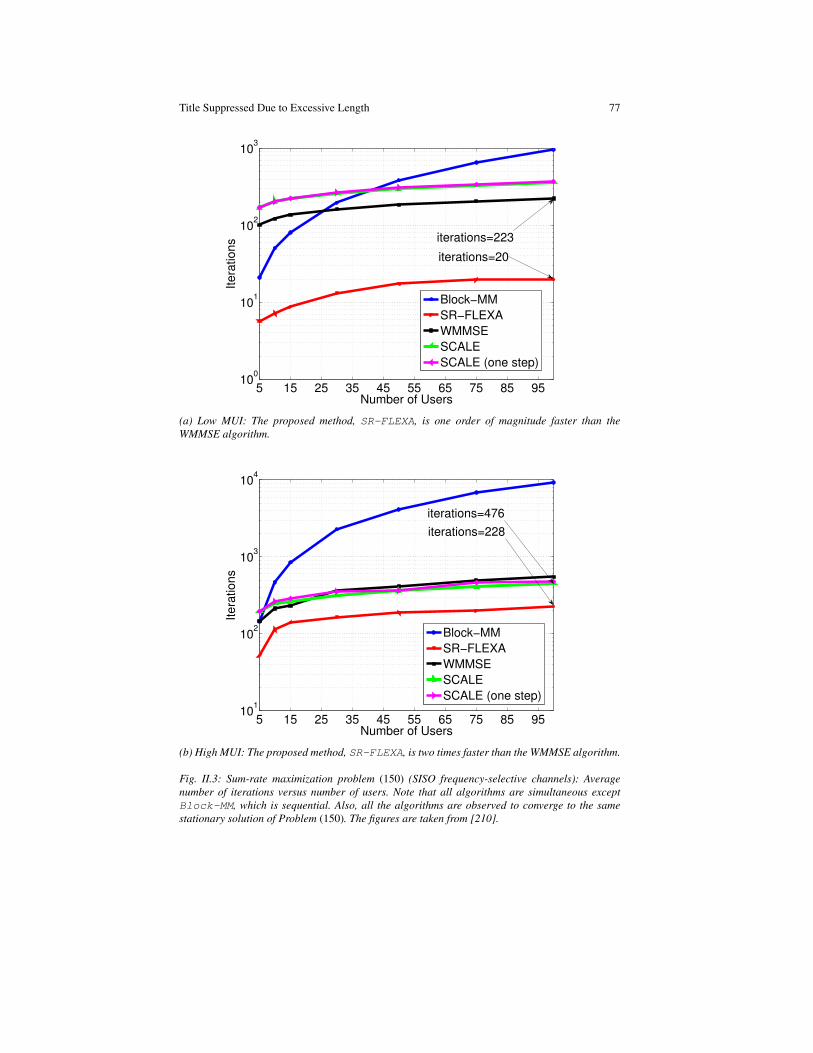
Title Suppressed Due to Excessive Length 77
5 15 25 35 45 55 65 75 85 9510
0
101
102
103
Number of Users
Itera
tions
Block−MM
SR−FLEXA
WMMSE
SCALE
SCALE (one step)
iterations=223
iterations=20
(a) Low MUI: The proposed method, SR-FLEXA, is one order of magnitude faster than theWMMSE algorithm.
5 15 25 35 45 55 65 75 85 9510
1
102
103
104
Number of Users
Itera
tions
Block−MM
SR−FLEXA
WMMSE
SCALE
SCALE (one step)
iterations=476
iterations=228
(b) High MUI: The proposed method, SR-FLEXA, is two times faster than the WMMSE algorithm.
Fig. II.3: Sum-rate maximization problem (150) (SISO frequency-selective channels): Averagenumber of iterations versus number of users. Note that all algorithms are simultaneous exceptBlock-MM, which is sequential. Also, all the algorithms are observed to converge to the samestationary solution of Problem (150). The figures are taken from [210].
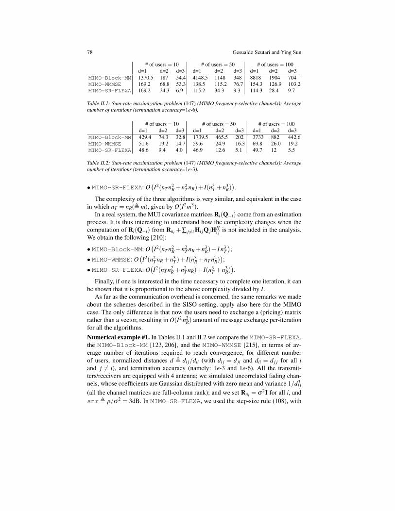
78 Gesualdo Scutari and Ying Sun
# of users = 10 # of users = 50 # of users = 100d=1 d=2 d=3 d=1 d=2 d=3 d=1 d=2 d=3
MIMO-Block-MM 1370.5 187 54.4 4148.5 1148 348 8818 1904 704MIMO-WMMSE 169.2 68.8 53.3 138.5 115.2 76.7 154.3 126.9 103.2MIMO-SR-FLEXA 169.2 24.3 6.9 115.2 34.3 9.3 114.3 28.4 9.7
Table II.1: Sum-rate maximization problem (147) (MIMO frequency-selective channels): Averagenumber of iterations (termination accuracy=1e-6).
# of users = 10 # of users = 50 # of users = 100d=1 d=2 d=3 d=1 d=2 d=3 d=1 d=2 d=3
MIMO-Block-MM 429.4 74.3 32.8 1739.5 465.5 202 3733 882 442.6MIMO-WMMSE 51.6 19.2 14.7 59.6 24.9 16.3 69.8 26.0 19.2MIMO-SR-FLEXA 48.6 9.4 4.0 46.9 12.6 5.1 49.7 12 5.5
Table II.2: Sum-rate maximization problem (147) (MIMO frequency-selective channels): Averagenumber of iterations (termination accuracy=1e-3).
• MIMO-SR-FLEXA: O(I2(nT n2
R +n2T nR)+ I(n3
T +n3R)).
The complexity of the three algorithms is very similar, and equivalent in the casein which nT = nR(, m), given by O(I2m3).
In a real system, the MUI covariance matrices Ri(Q−i) come from an estimationprocess. It is thus interesting to understand how the complexity changes when thecomputation of Ri(Q−i) from Rni +∑ j 6=i Hi jQ jHH
i j is not included in the analysis.We obtain the following [210]:
• MIMO-Block-MM: O(I2(nT n2
R +n2T nR +n3
R)+ I n3T);
• MIMO-WMMSE: O(I2(n2
T nR +n3T )+ I(n3
R +nT n2R));
• MIMO-SR-FLEXA: O(I2(nT n2
R +n2T nR)+ I(n3
T +n3R)).
Finally, if one is interested in the time necessary to complete one iteration, it canbe shown that it is proportional to the above complexity divided by I.
As far as the communication overhead is concerned, the same remarks we madeabout the schemes described in the SISO setting, apply also here for the MIMOcase. The only difference is that now the users need to exchange a (pricing) matrixrather than a vector, resulting in O(I2 n2
R) amount of message exchange per-iterationfor all the algorithms.Numerical example #1. In Tables II.1 and II.2 we compare the MIMO-SR-FLEXA,the MIMO-Block-MM [123, 206], and the MIMO-WMMSE [215], in terms of av-erage number of iterations required to reach convergence, for different numberof users, normalized distances d , di j/dii (with di j = d ji and dii = d j j for all iand j 6= i), and termination accuracy (namely: 1e-3 and 1e-6). All the transmit-ters/receivers are equipped with 4 antenna; we simulated uncorrelated fading chan-nels, whose coefficients are Gaussian distributed with zero mean and variance 1/d3
i j
(all the channel matrices are full-column rank); and we set Rni = σ2I for all i, andsnr , p/σ2 = 3dB. In MIMO-SR-FLEXA, we used the step-size rule (108), with

Title Suppressed Due to Excessive Length 79
ε = 1e-5; in (153) we set τi = 0 and computed Qi(Qk) using the closed form solutionin [123]. All the algorithms reach the same average sum-rate.
Given the results in Tables II.1 and II.2, the following comments are in order.MIMO-SR-FLEXA outperforms the other schemes in terms of iterations, while hav-ing similar (or even better) computational complexity. Interestingly, the iteration gapwith the other schemes reduces with the distance and the termination accuracy. Morespecifically: MIMO-SR-FLEXA i) seems to be much faster than the other schemes(about one order of magnitude) when di j/dii = 3 [say low interference scenarios],and just a bit faster (or comparable to MIMO-WMMSE) when di j/dii = 1 [say high in-terference scenarios]; and ii) it is much faster than the others, if an high terminationaccuracy is set (see Table II.1). Also, the convergence speed of MIMO-SR-FLEXAis not affected too much by the number of users. Finally, in our experiments, we alsoobserved that the performance of MIMO-SR-FLEXA is not affected too much by thechoice of the parameter ε in the (108): a change of ε of many orders of magnitudeleads to a difference in the average number of iterations which is within 5%; we referthe reader to [222] for details, where one can also find a comparison of several otherstep-size rules. We must stress however that MIMO-Block-MM and MIMO-WMMSEdo not need any tuning, which is an advantage with respect to MIMO-SR-FLEXA.Numerical example #2: We compare now the MIMO-WMMSE [215] and the MIMO-SR-FLEXA in a MIMO broadcast cellular system composed of multiple cells, withone Base Station (BS) and multiple randomly generated Mobile Terminals (MTs) ineach cell. Each MT experiences both intra-cell and inter-cell interference. We referto [215] for a detailed description of the system model, the explicit expressions ofthe BS-MT downlink rates, and the corresponding sum-rate maximization problem.
The setup of our experiments is the following [210]. We simulated seven cellswith multiple randomly generated MTs; each BS and MT is equipped with fourtransmit and receive antennas. Channels are Rayleigh fading, whose path-loss aregenerated using the 3 GPP(TR 36.814) methodology [1]. We assume white zero-mean Gaussian noise at each mobile receiver, with variance σ2, and same powerbudget p for all the BSs; the SNR is set to snr , p/σ2 = 3dB. Both algo-rithms MIMO-WMMSE and MIMO-SR-FLEXA are initialized by choosing the samefeasible randomly generated point, and are terminated when (the absolute valueof) the sum-rate error in two consecutive rounds becomes smaller than 1e-2. InMIMO-SR-FLEXA, the step-size rule (108) is used, with ε = 1e-3 and γ0 = 1; theunique solution Qi(Qk) of users’ subproblems is computed in closed form adapt-ing the procedure in [123]. The experiments were run using Matlab R2012a on a12× 2.40 GHz Intel Xeon E5645 Processor Cores machine, equipped with 48 GBof memory and 24576 Kbytes of data cache; the operation system is Linux (Red-Hat Enterprise Linux 6.1 2.6.32 Kernel). In Fig. II.4a we plot the average cpu timeversus the total number of MTs for the two algorithms under the same terminationcriterion, whereas in Fig. II.4b we reported the final achieved average sum-rate. Thecurves are averaged over 1500 channel/topology realizations. It can be observedthat MIMO-SR-FLEXA significantly outperforms MIMO-WMMSE in terms of cputime when the number of active users is large; moreover MIMO-SR-FLEXA also
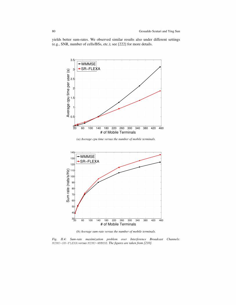
80 Gesualdo Scutari and Ying Sun
yields better sum-rates. We observed similar results also under different settings(e.g., SNR, number of cells/BSs, etc.); see [222] for more details.
20 60 100 140 180 220 260 300 340 380 420 4600
0.5
1
1.5
2
2.5
3
3.5
# of Mobile Terminals
Avera
ge c
pu tim
e p
er
user
(s)
WMMSE
SR−FLEXA
(a) Average cpu time versus the number of mobile terminals.
20 60 100 140 180 220 260 300 340 380 420 46030
40
50
60
70
80
90
100
110
120
130
140
# of Mobile Terminals
Sum
rate
(nats
/s/H
z)
WMMSE
SR−FLEXA
(b) Average sum-rate versus the number of mobile terminals.
Fig. II.4: Sum-rate maximization problem over Interference Broadcast Channels:MIMO-SR-FLEXA versus MIMO-WMMSE. The figures are taken from [210].
Title Suppressed Due to Excessive Length 81
II.5.2 LASSO problem
Consider the LASSO problem in the following form [235] (cf. Sec. II.1.1):
minimizex
V (x),12‖z−Ax‖2 +λ‖x‖1, (154)
where A ∈ Rq×m is the matrix whose columns ai are the prediction or feature vec-tors; zi is the response variable associated to ai; and λ > 0 is the regularizationweight.FLEXA for LASSO. Observing that the univariate instance of (154) has a closedform solution, it is convenient to decompose x in scalar components (mi = 1, for alli ∈ N) and update them in parallel. In order to exploit the quadratic structure of V in(154) a natural choice for the surrogate function is (102). Therefore, the subproblemassociated with the scalar xi reads: given xk,
xi(xk), argminxi∈R
12
∥∥∥rki −ai xi
∥∥∥2+
τi
2· (xi− xk
i )2 +λ · |xi|
,
where the residual rki is defined as
rki , z−∑
j 6=ia j xk
j.
Invoking the first order optimality conditions (c.f. Def. I.9) [we write xi for xi(xk)]:
−(
aTi rk
i + τi xki
)+(τi +‖ai‖2) xi +λ ∂ |xi| 3 0,
and the expression of ∂ |x| [cf. (9)], one can readily obtain the closed form expressionof xi(xk), that is,
xi(xk) =1
τi +‖ai‖2 ·Sλ
(aT
i rki + τi xk
i
), (155)
where Sλ (•) is the soft-thresholding operator, defined in (54).We consider the instance of Algorithm 6, with the following choice of the free
parameters:
• Exact solution xi(xk): In Step 3 we use the best-response xi(xk) as defined in(155), that is, zk
i = xi(xk) (exact solution).• Proximal weights τi: While in the proposed algorithmic framework we consid-
ered fixed values of τi, varying τi a finite number of times does not affect thetheoretical convergence properties of the algorithms. We found that the follow-ing choices work well in practice: (i) τi are initially all set to τi = tr(AT A)/(2m),i.e., to half of the mean of the eigenvalues of ∇2F ; (ii) all τi are doubled if at acertain iteration the objective function does not decrease; and (iii) they are allhalved if the objective function decreases for ten consecutive iterations or therelative error on the objective function re(x) is sufficiently small, specificallyif
82 Gesualdo Scutari and Ying Sun
re(x),V (x)−V ∗
V ∗≤ 10−2, (156)
where V ∗ is the optimal value of the objective function V (in our experiments onLASSO, V ∗ is known). In order to avoid increments in the objective function,whenever all τi are doubled, the associated iteration is discarded, and in Step 4of Algorithm 6 it is set xk+1 = xk. In any case we limited the number of possibleupdates of the values of τi to 100.
• Step-size γk: The step-size γk is updated according to the following rule:
γk = γ
k−1(
1−min
1,10−4
re(xk)
θ γ
k−1), k = 1, . . . , (157)
with γ0 = 0.9 and θ = 1e− 7. The above diminishing rule is based on (108)while guaranteeing that γk does not become too close to zero before the relativeerror is sufficiently small.
• Greedy selection rule Sk: In Step 2, we use the following greedy selection rule(satisfying Assumption II.10.2):
Sk = i : Ei(xk)≥ σ ·Mk, with Ei(xk) = |xi(xk)− xki |.
In our tests we consider two options for σ , namely: i) σ = 0, which leads toa fully parallel scheme wherein at each iteration all variables are updated; andii) σ = 0.5, which corresponds to updating only a subset of all the variables ateach iteration. Note that for both choices of σ , the resulting set Sk satisfies therequirement in Step 2 of Algorithm 6; indeed, Sk always contains the index icorresponding to the largest Ei(xk). We will refer to these two instances of thealgorithm as FLEXA σ = 0 and FLEXA σ = 0.5.
Algorithms in the literature: We compared the above versions of FLEXA with themost competitive parallel and sequential (Block MM) algorithms proposed in theliterature to solve the LASSO problem. More specifically, we consider the followingschemes.• FISTA: The Fast Iterative Shrinkage-Thresholding Algorithm (FISTA) proposedin [7] is a first order method and can be regarded as the benchmark algorithm forLASSO problems. Building on the separability of the terms in the objective func-tion V , this method can be easily parallelized and thus take advantage of a parallelarchitecture. We implemented the parallel version that use a backtracking procedureto estimate the Lipschitz constant of ∇F [7].• SpaRSA: This is the first order method proposed in [251]; it is a popular spectralprojected gradient method that uses a spectral step length together with a nonmono-tone line search to enhance convergence. Also this method can be easily parallelized,which is the version implemented in our tests. In all the experiments, we set the pa-rameters of SpaRSA as in [251]: M = 5, σ = 0.01, αmax = 1e30, and αmin = 1e−30.• GRock & Greedy-1BCD: GRock is a parallel algorithm proposed in [187]that performs well on sparse LASSO problems. We tested the instance of GRockwhere the number of variables simultaneously updated is equal to the number of
Title Suppressed Due to Excessive Length 83
the parallel processors. It is important to remark that the theoretical convergenceproperties of GRock are in jeopardy as the number of variables updated in parallelincreases; roughly speaking, GRock is guaranteed to converge if the columns ofthe data matrix A in the LASSO problem are “almost” orthogonal, a feature that ingeneral is not satisfied by real data. A special instance with convergence guaranteedis the one where only one block per time (chosen in a greedy fashion) is updated;we refer to this special case as greedy-1BCD.• Parallel ADMM: This is a classical Alternating Method of Multipliers (ADMM).We implemented the parallel version proposed in [67].
In the implementation of the parallel algorithms, the data matrix A of the LASSOproblem is generated as follows. Each processor generates a slice of the matrix itselfsuch that A = [A1 A2 · · · AP], where P is the number of parallel processors, and eachAi has m/P columns. Thus the computation of each product Ax (which is requiredto evaluate ∇F) and the norm ‖x‖1 (that is G) is divided into the parallel jobs ofcomputing Ai xi and ‖xi‖1, followed by a reducing operation.Numerical examples. We generated six groups of LASSO problems using the ran-dom generator proposed by Nesterov [172], which permits to control the sparsity ofthe solution. For the first five groups, we considered problems with 10,000 variablesand matrices A with 9,000 rows. The five groups differ in the degree of sparsity ofthe solution, namely: the percentage of non zeros in the solution is 1%, 10%, 20%,30%, and 40%, respectively. The last group is formed by instances with 100,000variables and 5000 rows for A, and solutions having 1% of non zero variables. In allexperiments and for all the algorithms, the initial point was set to the zero vector.
Results of the experiments for the 10,000 variables groups are reported in Fig.II.5, where we plot the relative error as defined in (156) versus the CPU time; allthe curves are obtained using (up to) 40 cores, and averaged over ten independentrandom realizations. Note that the CPU time includes communication times (forparallel algorithms) and the initial time needed by the methods to perform all pre-iteration computations (this explains why the curves of ADMM start after the others;in fact ADMM requires some nontrivial initializations). For one instance, the onecorresponding to 1% of the sparsity of the solution, we plot also the relative errorversus iterations [Fig. II.5(a2)]; similar behaviors of the algorithms have been ob-served also for the other instances, and thus are not reported. Results for the LASSOinstance with 100,000 variables are plotted in Fig. II.6. The curves are averaged overfive random realizations.
The following comments are in order. On all the tested problems, FLEXAσ = 0.5 outperforms in a consistent manner all the other implemented algorithms.In particular, as the sparsity of the solution decreases, the problems become harderand the selective update operated by FLEXA σ = 0.5 improves over FLEXA σ = 0,where instead all variables are updated at each iteration. FISTA is capable to ap-proach relatively fast low accuracy when the solution is not too sparse, but has dif-ficulties in reaching high accuracy. SpaRSA seems to be very insensitive to thedegree of sparsity of the solution; it behaves well on 10,000 variables problems andnot too sparse solutions, but is much less effective on very large-scale problems.The version of GRock with P = 40 is the closest match to FLEXA, but only when
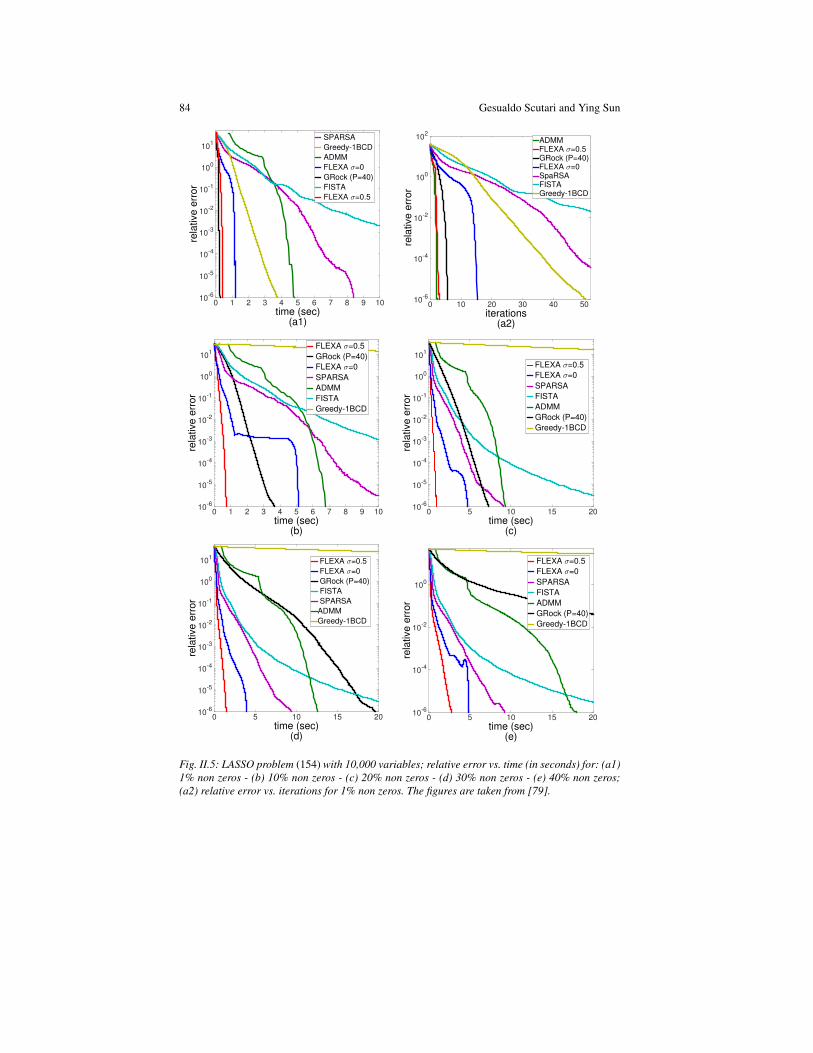
84 Gesualdo Scutari and Ying Sun
time (sec)(a1)
0 1 2 3 4 5 6 7 8 9 10
rela
tive e
rror
10-6
10-5
10-4
10-3
10-2
10-1
100
101
SPARSA
Greedy-1BCD
ADMM
FLEXA σ=0
GRock (P=40)
FISTA
FLEXA σ=0.5
iterations (a2)
0 10 20 30 40 50
rela
tive e
rror
10-6
10-4
10-2
100
102
ADMMFLEXA σ=0.5GRock (P=40)FLEXA σ=0SpaRSAFISTAGreedy-1BCD
time (sec)(b)
0 1 2 3 4 5 6 7 8 9 10
rela
tive e
rror
10-6
10-5
10-4
10-3
10-2
10-1
100
101
FLEXA σ=0.5
GRock (P=40)
FLEXA σ=0
SPARSA
ADMM
FISTA
Greedy-1BCD
time (sec)(c)
0 5 10 15 20
rela
tive e
rror
10-6
10-5
10-4
10-3
10-2
10-1
100
101
FLEXA σ=0.5
FLEXA σ=0
SPARSA
FISTA
ADMM
GRock (P=40)
Greedy-1BCD
time (sec)(d)
0 5 10 15 20
rela
tive e
rror
10-6
10-5
10-4
10-3
10-2
10-1
100
101
FLEXA σ=0.5
FLEXA σ=0
GRock (P=40)
FISTA
SPARSA
ADMM
Greedy-1BCD
time (sec)(e)
0 5 10 15 20
rela
tive e
rror
10-6
10-4
10-2
100
FLEXA σ=0.5
FLEXA σ=0
SPARSA
FISTA
ADMM
GRock (P=40)
Greedy-1BCD
Fig. II.5: LASSO problem (154) with 10,000 variables; relative error vs. time (in seconds) for: (a1)1% non zeros - (b) 10% non zeros - (c) 20% non zeros - (d) 30% non zeros - (e) 40% non zeros;(a2) relative error vs. iterations for 1% non zeros. The figures are taken from [79].

Title Suppressed Due to Excessive Length 85
time (sec) (a)
0 100 200 300 400
rela
tive e
rror
10-6
10-4
10-2
100
102
ADMM
SpaRSA
FLEXA σ = 0.5
FISTA
FLEXA σ = 0
GRock (P = 8)
Greedy-1BCD
time (sec) (b)
0 100 200 300 400
rela
tive e
rror
10-6
10-4
10-2
100
102
ADMM
FLEXA σ = 0
FLEXA σ = 0.5
FISTA
SpaRSA
Greedy-1BCD
GRock (P=20)
Fig. II.6: LASSO problem (154) with 105 variables; Relative error vs. time for: (a) 8 cores - (b) 20cores. The figures are taken from [79].
the problems are very sparse (but it is not supported by a convergence theory onour test problems). This is consistent with the fact that its convergence propertiesare at stake when the problems are quite dense. Furthermore, if the problem is verylarge, updating only 40 variables at each iteration, as GRock does, could slow downthe convergence, especially when the optimal solution is not very sparse. From thispoint of view, FLEXA σ = 0.5 seems to strike a good balance between not updatingvariables that are probably zero at the optimum and nevertheless update a sizeableamount of variables when needed in order to enhance convergence.
Remark II.21 (On the parallelism). Fig. II.6 shows that FLEXA seems to exploitwell parallelism on LASSO problems. Indeed, when passing from 8 to 20 cores,the running time approximately halves. This kind of behavior has been consistentlyobserved also for smaller problems and different number of cores (not reportedhere). Note that practical speed-up due to the use of a parallel architecture is givenby several factor that are not easily predictable, including communication timesamong the cores, the data format, etc.. Here we do not pursue a theoretical study ofthe speed-up but refer to [37] for some initial study. We finally observe that GRockappears to improve greatly with the number of cores. This is due to the fact thatin GRock the maximum number of variables that is updated in parallel is exactlyequal to the number of cores (i.e., the degree of parallelism), and this might becomea serious drawback on very large problems (on top of the fact that convergence is injeopardy). On the contrary, the theory presented in this chapter permits the parallelupdate of any number of variables while guaranteeing convergence.
Remark II.22 (On selective updates). It is interesting to comment why FLEXAσ = 0.5 behaves better than FLEXA σ = 0. To understand the reason behind thisphenomenon, we first note that Algorithm 6 has the remarkable capability to iden-tify those variables that will be zero at a solution; we do not provide here the proofof this statement but only an informal argument. Roughly speaking, it can be shown
86 Gesualdo Scutari and Ying Sun
that, for k large enough, those variables that are zero in x(xk) = (xi(xk))mi=1 will
be zero also in a limiting solution x. Therefore, suppose that k is large enough sothat this identification property already takes place (we will say that “we are in theidentification phase”) and consider an index i such that xi = 0. Then, if xk
i is zero,it is clear, by Steps 3 and 4, that xk′
i will be zero for all indices k′ > k, indepen-dently of whether i belongs to Sk or not. In other words, if a variable that is zeroat the solution is already zero when the algorithm enters the identification phase,that variable will be zero in all subsequent iterations; this fact, intuitively, shouldenhance the convergence speed of the algorithm. Conversely, if when we enter theidentification phase xk
i is not zero, the algorithm will have to bring it back to zeroiteratively. This explains why updating only variables that we have “strong” reasonto believe will be non zero at a solution is a better strategy than updating them all.Of course, there may be a problem dependence and the best value of σ can varyfrom problem to problem. But the above explanation supports the idea that it mightbe wise to “waste" some calculations and perform only a partial ad-hoc update ofthe variables.
II.5.3 The logistic regression problemConsider the logistic regression problem in the following form [235]:
minimizex
V (x) =q
∑i=1
log(1+ e−wi·zTi x)+λ‖x‖1, (158)
where zi ∈ Rm is the feature vector of sample i, with the associated label wi ∈−1,1.FLEXA for logistic regression. Problem (158) is a highly nonlinear problem in-volving many exponentials that, notoriously, gives rise to numerical difficulties.Because of these high nonlinearities, a Gauss-Seidel (sequential) approach is ex-pected to be more effective than a pure Jacobi (parallel) method, a fact that wasconfirmed by the experiments in [79]. For this reason, for the logistic regressionproblem we tested both FLEXA and the hybrid scheme in Algorithm 9, which willterm GJ-FLEXA. The setting of the free parameters in GJ-FLEXA is essentiallythe same as the one described for LASSO (cf. Sec. II.5.2), but with the followingdifferences:
• Exact solution xi(xk): The surrogate function Fi is chosen as the second orderapproximation of the original function F : given the current iterate xk,
Fi(xi |xk)=F(xk)+∇xiF(xk) ·(xi−xki )+
12(∇2
xi xiF(xk)+τi) ·(xi−xk
i )2+λ · |xi|,
which leads to the following closed form solution for xi(xk):
xi(xk) = Sλ ·tk
i
(xk
i − tki ·∇xiF(xk)
), with tk
i ,(
τi +∇2xi xi
F(xk))−1
,
where Sλ (•) is the soft-thresholding operator, defined in (54).

Title Suppressed Due to Excessive Length 87
• Proximal weights τi: The initial τi are set to tr(ZT Z)/(2m), for all i, where m isthe total number of variables and Z = [z1 z2 · · · zq]
T .
• Step-size γk: We use the step-size rule (157). However, since the optimal valueV ∗ is not known for the logistic regression problem, re(x) can no longer becomputed. We replace re(x) with the merit function ‖M(x)‖∞, with
M(x), ∇F(x)−Π[−λ ,λ ]m (∇F(x)−x) .
Here the projection Π[−λ ,λ ]m(y) can be efficiently computed; it acts component-wise on y, since [−λ ,λ ]m = [−λ ,λ ]×·· ·× [−λ ,λ ]. Note that M(x) is a validoptimality measure function; indeed, it is continuous and M(x)= 0 is equivalentto the standard necessary optimality condition for Problem (94), see [31].
Algorithms in the literature: We compared FLEXA (σ = 0.5) (cf. Sec. II.5.2)and GJ-FLEXA with the other parallel algorithms introduced in Sec. II.5.2 forthe LASSO problem (whose tuning of the free parameters is the same as in Fig.II.5 and Fig. II.6), namely: FISTA, SpaRSA, and GRock. For the logistic regres-sion problem, we also tested one more algorithm, that we call CDM. This Coor-dinate Descent Method is an extremely efficient Gauss-Seidel-type method (cus-tomized for logistic regression), and is part of the LIBLINEAR package available athttp://www.csie.ntu.edu.tw/~cjlin/.
We tested the aforementioned algorithms on three instances of the logistic re-gression problem that are widely used in the literature, and whose essential datafeatures are given in Table II.3; we downloaded the data from the LIBSVM repos-itory http://www.csie.ntu.edu.tw/~cjlin/libsvm/, which we referto for a detailed description of the test problems. In our implementation, the ma-trix Z is column-wise partitioned according to Z =
[Z1 Z2 · · · ZP
]and distributively
stored across P processors, where Zi is the set of columns of Z owned by processori.
In Fig. II.7, we plotted the relative error vs. the CPU time (the latter defined asin Fig. II.5 and Fig. II.6) achieved by the aforementioned algorithms for the threedatasets, and using a different number of cores, namely: 8, 16, 20, 40; for each algo-rithm but GJ-FLEXA we report only the best performance over the aforementionednumbers of cores. Note that in order to plot the relative error, we had to preliminaryestimate V ∗ (which is not known for logistic regression problems). To do so, we ranGJ-FLEXA until the merit function value ‖M(xk)‖∞ went below 10−7, and usedthe corresponding value of the objective function as estimate of V ∗. We remark thatwe used this value only to plot the curves. Next to each plot, we also reported theoverall FLOPS counted up till reaching the relative errors as indicated in the table.Note that the FLOPS of GRock on real-sim and rcv1 are those counted in 24 hourssimulation time; when terminated, the algorithm achieved a relative error that wasstill very far from the reference values set in our experiment. Specifically, GRockreached 1.16 (instead of 1e−4) on real-sim and 0.58 (instead of 1e−3) on rcv1; thecounted FLOPS up till those error values are still reported in the tables.
The analysis of the figures shows that, due to the high nonlinearities of the objec-tive function, Gauss-Seidel-type methods outperform the other schemes. In spite of

88 Gesualdo Scutari and Ying Sun
time (sec)0 100 200 300 400 500 600
rela
tive e
rror
10-6
10-4
10-2
100
102
Gisette (6000x5000)
CDM
FLEXA GJ (1 core)
FLEXA GJ (20 cores)
SpaRSA (20 cores)
FLEXA σ = 0.5 (20 cores)
FISTA (20 cores)
GRock (P = 20, 20 cores)
Algorithms FLOPS (1e-2/1e-6)GJ-FLEXA (1C) 1.30e+10/1.23e+11GJ-FLEXA (20C) 5.18e+11/5.07e+12
FLEXA σ =0.5 (20C) 1.88e+12/4.06e+13CDM 2.15e+10/1.68e+11
SpaRSA (20C) 2.20e+12/5.37e+13FISTA (20C) 3.99e+12/5.66e+13GRock (20C) 7.18e+12/1.81e+14
time (sec)0 20 40 60 80
rela
tive e
rror
10-6
10-5
10-4
10-3
10-2
10-1
100
101
Real Sim (72309x20958)
CDM
FLEXA GJ(20 cores)
FISTA (20 cores)
GRock (P=20, 20 cores)
SpaRSA (20 cores)
FLEXA GJ (1 core)
FLEXA GJ (8 cores)
FLEXA σ = 0.5 (20 cores)
Algorithms FLOPS (1e-4/1e-6)GJ-FLEXA (1C) 2.76e+9/6.60e+9GJ-FLEXA (20C) 9.83e+10/2.85e+11
FLEXA σ =0.5 (20C) 3.54e+10/4.69e+11CDM 4.43e+9/2.18e+10
SpaRSA (20C) 7.18e+9/1.94e+11FISTA (20C) 3.91e+10/1.56e+11GRock (20C) 8.30e+14 (after 24h)
time (sec)0 200 400 600 800 1000
rela
tive e
rror
10-6
10-4
10-2
100
102
Rcv (67739x47236)
FLEXA GJ(1 core)
FLEXA GJ (20 cores)
FLEXA σ=0.5 (20C cores)
CDM
GRock (20 cores)
SPARSA (20 cores)
FISTA (20 cores)
Algorithms FLOPS (1e-3/1e-6)GJ-FLEXA (1C) 3.61e+10/2.43e+11GJ-FLEXA (20C) 1.35e+12/6.22e+12
FLEXA σ =0.5 (20C) 8.53e+11/7.19e+12CDM 5.60e+10/6.00e+11
SpaRSA (20C) 9.38e+12/7.20e+13FISTA (20C) 2.58e+12/2.76e+13GRock (20C) 1.72e+15 (after 24h)
Fig. II.7: Logistic Regression problem (158): Relative error vs. time (in seconds) and FLOPS fori) gisette, ii) real-sim, and iii) rcv. The figures are taken from [79].

Title Suppressed Due to Excessive Length 89
Data set q m λ
gisette (scaled) 6000 5000 0.25real-sim 72309 20958 4
rcv1 677399 47236 4
Table II.3: Data sets for the logistic regression tests [Problem (158)]
this, FLEXA still behaves quite well. But GJ-FLEXA with one core, thus a non par-allel method, clearly outperforms all other algorithms. The explanation can be thefollowing. GJ-FLEXA with one core is essentially a Gauss-Seidel-type method butwith two key differences: the use of a stepsize and more importantly a (greedy) se-lection rule by which only some variables are updated at each round. As the numberof cores increases, the algorithm gets “closer and closer” to a Jacobi-type method,and because of the high nonlinearities, moving along a “Jacobi direction” does notbring improvements. In conclusion, for logistic regression problems, our experi-ments suggests that while the (opportunistic) selection of variables to update seemsuseful and brings to improvements even in comparison to the extremely efficient,dedicated CDM algorithm/software, parallelism (at least, in the form embedded inour scheme), does not appear to be beneficial as instead observed for LASSO prob-lems.
II.6. Appendix
II.6.1 Proof of Lemma II.4
The continuity of x(•) follows readily from [199]; see also [104].We prove next the Lipschitz continuity of x(•), under the additional assumption
that G is separable. Let xi,zi ∈ Xi. Invoking the optimality conditions of xi(x) andxi(z), we have
(y1− xi(x))T (∇Fi(xi(x) |x))+gi(y1)−gi(xi(x))≥ 0, ∀y1 ∈ Xi,
(y2− xi(z))T (∇Fi(xi(z) |z))+gi(y2)−gi(xi(z))≥ 0, ∀y2 ∈ Xi.
Letting y1 = xi(z) and y2 = xi(x) and summing the two inequalities above, we obtain
(xi(z)− xi(x))T(
∇Fi(xi(x) |x)−∇Fi(xi(z) |z))≥ 0.
Adding and subtracting ∇Fi(xi(z) |x) and using the uniform strongly convexity of Fiwith respect to its first argument (cf. Assumption II.2.1) and the Lipschitz continuityof ∇Fi with respect to its second argument (cf. Assumption II.3) yield
τi ‖xi(z)− xi(x)‖2 ≤ (xi(z)− xi(x))T (∇Fi(xi(z) |x)−∇Fi(xi(z) |z))≤ Li ‖xi(z)− xi(x)‖ · ‖x− z‖.

90 Gesualdo Scutari and Ying Sun
Therefore, xi(•) is Lipschitz continuous on X with constant Li , Li/τi.
II.6.2 Proof of Lemma II.17
The proof is adapted by [56, Lemma 10] and reported here for completeness.With a slight abuse of notation, we will use (xi,x j,y−(i, j)), with i < j, to denote
the ordered tuple (y1, . . . ,yi−1,xi,yi+1, . . . ,y j−1,x j,y j+1, . . . ,yn).Given k ≥ 0, Sk ⊆ N, and γk ≤ 1/n, let γk = γkn ≤ 1. Define xk , (xk
i )i∈N , withxk
i = xki if i /∈ Sk, and
xki , γ
k zki +(1− γ
k)xki , (159)
otherwise. Then xk+1 in Step 4 of the algorithm can be written as
xk+1 =n−1
nxk +
1n
xk. (160)
Using (160) and invoking the convexity of G, the following recursion holds for allk:
G(xk+1) = G(
1n(xk
1,xk−1)+
1n(xk
1, xk−1)+
n−2n
xk)
= G(
1n(xk
1,xk−1)+
n−1n
(xk
1,1
n−1xk−1 +
n−2n−1
xk−1
))≤ 1
nG(
xk1,x
k−1
)+
n−1n
G(
xk1,
1n−1
xk−1 +
n−2n−1
xk−1
)=
1n
G(
xk1,x
k−1
)+
n−1n
G(
1n−1
(xk
1, xk−1
)+
n−2n−1
xk)
=1n
G(
xk1,x
k−1
)+
n−1n
G(
1n−1
(xk
2,xk−2
)+
1n−1
(xk
1,xk2, x
k−(1,2)
)+
n−3n−1
xk)
=1n
G(
xk1,x
k−1
)+
n−1n
G(
1n−1
(xk
2,xk−2
)+
n−2n−1
(xk
1,xk2,
1n−2
xk−(1,2)+
n−3n−2
xk−(1,2)
))≤ 1
nG(
xk1,x
k−1
)+
1n
G(
xk2,x
k−2
)+
n−2n
G(
xk1,x
k2,
1n−2
xk−(1,2)+
n−3n−2
xk−(1,2)
)≤ ·· · ≤ 1
n ∑i∈N
G(xki ,x
k−i).
(161)
Using (161), the difference of G(xk+1) and G(xk) can be bounded as

Title Suppressed Due to Excessive Length 91
G(xk+1)−G(xk)≤ 1n ∑
i∈N
(G(xk
i ,xk−i)−G(xk)
)=
1n ∑
i∈Sk
(G(xk
i ,xk−i)−G(xk)
)(162)
≤ 1n ∑
i∈Sk
(γ
kG(zki ,x
k−i)+(1− γ
k)G(xk)−G(xk))
= γk∑
i∈Sk
(G(zk
i ,xk−i)−G(xk)
).
II.6.3 Proof of Lemma II.19
The proof can be found in [79, Lemma 10], and reported here for completeness.For notational simplicity, we will write xSk for (x)Sk [recall that (x)Sk denotes the
vector whose block component i is equal to xi if i ∈ Sk, and zero otherwise]. Let jkbe an index in Sk such that E jk(x
k)≥ ρ maxi Ei(xk) (cf. Assumption II.10.2). Then,by the error bound condition (110) it is easy to check that the following chain ofinequalities holds:
s jk‖xSk(xk)−xkSk‖ ≥ s jk‖x jk(x
k)−xkjk‖
≥ E jk(xk)
≥ ρ maxi
Ei(xk)
≥(
ρ mini
si
)(max
i‖xi(xk)−xk
i ‖)
≥(
ρ mini si
n
)‖x(xk)−xk‖.
Hence we have for any k,
‖xSk(xk)−xkSk‖ ≥
(ρ mini si
ns jk
)‖x(xk)−xk‖ ≥
(ρ mini si
nmax j s j
)‖x(xk)−xk‖.
92 Gesualdo Scutari and Ying Sun
II.7. Sources and NotesAlthough parallel (deterministic and stochastic) block-methods have a long history(mainly for convex problems), recent years have witnessed a revival of such methodsand their (probabilistic) analysis; this is mainly due to the current trend towardshuge scale optimization and the availability of ever more complex computationalarchitectures that call for efficient, fast, and resilient algorithms. The literature isvast and a comprehensive overview of current methods goes beyond the scope of thiscommentary. Here we only focus on SCA-related methods and refer to [25,214,250](and references therein) as entry point to other numerical optimization algorithms.Parallel SCA-related Methods: The roots of parallel deterministic SCA schemes(wherein all the variables are updated simultaneously) can be traced back at leastto the work of Cohen on the so-called auxiliary principle [51, 52] and its re-lated developments, see e.g. [7, 28, 89, 162, 165, 172, 183, 187, 197, 210, 238, 251].Roughly speaking, these works can be divided in two groups, namely: parallel so-lution methods for convex objective functions [7, 28, 51, 52, 165, 187, 197] and non-convex ones [89, 162, 172, 183, 210, 238, 251]. All methods in the former group(and [89, 162, 172, 238, 251]) are (proximal) gradient schemes; they thus sharethe classical drawbacks of gradient-like schemes; moreover, by replacing the con-vex function F with its first order approximation, they do not take any advan-tage of any structure of F beyond mere differentiability. Exploiting some avail-able structural properties of F , instead, has been shown to enhance (practical)convergence speed, see e.g. [210]. Comparing with the second group of works[89, 162, 172, 183, 210, 238, 251], the parallel SCA algorithmic framework intro-duced in this lecture improves on their convergence properties while adding greatflexibility in the selection of the variables to update at each iteration. For instance,with the exception of [68, 143, 187, 204, 238], all the aforementioned works do notallow parallel updates of a subset of all variables, a feature that instead, fully ex-plored as we do, can dramatically improve the convergence speed of the algorithm,as shown in Sec. II.5. Moreover, with the exception of [183], they all require anArmijo-type line-search, whereas the scheme in [183] is based on diminishing step-size-rules, but its convergence properties are quite weak: not all the limit points ofthe sequence generated by this scheme are guaranteed to be stationary solutions of(94).
The SCA-based algorithmic framework introduced in this lecture builds on andgeneralizes the schemes proposed in [56, 79, 210]. More specifically, Algorithm 5was proposed in [210] for smooth instances of Problem (94) (i.e., G = 0); con-vergence was established when constant (Assumption II.11.1) or diminishing (As-sumption II.11.2) step-sizes are employed (special case of Theorem II.8). In [79],this algorithm was extended to deal with nonsmooth separable functions G whileincorporating inexact updates (Assumption II.9.1) and the greedy selection rule inAssumption II.10.2 (cf. Algorithm 6) as well as hybrid Jacobi/Gauss-Seidel up-dates (as described in Algorithm 8); convergence was established under Assump-tion II.11.2 (diminishing step-size) (special case of Theorem II.12). Finally, in [56],an instance of Algorithm 6 was proposed, to deal with nonseparable convex func-

Title Suppressed Due to Excessive Length 93
tions G, and using random block selection rules (Assumption II.10.4) or hybridrandom-greedy selection rules (Algorithm 7); convergence was established when adiminishing step-size is employed (special case of Theorem II.13).
While [56, 79, 210] studied some instances of parallel SCA methods in isolation(and only for some block selection rules and step-size rules) the contribution of thislecture is to provide a broader and unified view and analysis of such methods.SCA Methods for nonconvex constrained optimization: (Parallel) SCA methodshave been recently extended to deal with nonconvex constraints; state-of-the-art de-velopments can be found in [76, 77, 207] along with their applications to some rep-resentative problems in Signal Processing, Communications, and Machine Learn-ing [208]. More specifically, consider the following generalization of Problem (94):
minimizex
F(x)+H(x)s.t. x ∈ X ,
g j(x)≤ 0, j = 1, . . . ,J,
(163)
where g j(x)≤ 0, j = 1, . . . ,J, represent nonconvex nonsmooth constraints; and H isnow a nonsmooth, possibly nonconvex function.
A natural extension of the SCA idea introduced in this lecture to the general classof nonconvex problems (163) is replacing all the nonconvex functions with suitablychosen convex surrogates, and solve instead the following convexified problems:given xk,
x(xk), argminx
F(x |xk)+ H(x |xk)
s.t. x ∈ X ,
g j(x |y)≤ 0, j = 1, . . . ,J;
(164)
where F , H and g j are (strongly) convex surrogates for F , H, and g j, respectively.The update of xk is then given by
xk+1 = xk+1 + γk(
x(xk)−xk).
Conditions on the surrogates in (164) and convergence of the resulting SCA al-gorithms can be found in [207] for the case of smooth H and g j (or nonsmoothDC), and in [77] for the more general setting of nonsmooth functions; parallel anddistributed implementations are also discussed. Here we only mention that the sur-rogates g j must be a global convex upper bound of the associated nonconvex g j (asfor the MM algorithms–see Lecture I). This condition was removed in [76] wherea different structure for the subproblems (164) was proposed. The work [76] alsoprovides a complexity analysis of the SCA-based algorithms.
Other SCA-related methods for nonconvex constrained problem are discussedin [76, 77, 207, 208], which we refer to for details.Asynchronous SCA methods: In the era of data deluge, data-intensive applicationsgive rise to extremely large-scale problems, which naturally call for asynchronous,parallel solution methods. In fact, well suited to modern computational architec-

94 Gesualdo Scutari and Ying Sun
tures (e.g., shared memory systems, message passing-based systems, cluster com-puters, cloud federations), asynchronous methods reduce the idle times of workers,mitigate communication and/or memory-access congestion, and make algorithmsmore fault-tolerant. Although asynchronous block-methods have a long history (see,e.g., [5, 16, 45, 87, 237]), in the past few years, the study of asynchronous paralleloptimization methods has witnessed a revival of interest. Indeed, asynchronous par-allelism has been applied to many state-of-the-art optimization algorithms (mainlyfor convex objective functions and constraints), including stochastic gradient meth-ods [109,137,144,153,167,184,195] and ADMM-like schemes [105,110,247]. Theasynchronous counterpart of BCD methods has been introduced and studied in theseminal work [146], which motivated and oriented much of subsequent research inthe field, see e.g. [60, 61, 147, 185, 186].
Asynchronous parallel SCA methods were recently proposed and analyzed in[37, 38] for nonconvex problems in the form (94), with G separable and Xi possiblynonconvex [we refer to such a class of problems as Problem (94)′]. In the asyn-chronous parallel SCA method [37, 38], workers (e.g., cores, cpus, or machines)continuously and without coordination with each other, update a block-variable bysolving a strongly convex block-model of Problem (94)′. More specifically, at itera-tion k, a worker updates a block-variable xk
ik of xk to xk+1ik
, with ik in the set N, thusgenerating the vector xk+1. When updating block ik, in general, the worker doesnot have access to the current vector xk, but it will use instead the local estimate
xk−dk, (x
k−dk1
1 ,xk−dk
22 , . . . ,xk−dk
nn ), where dk , (dk
1,dk2, . . . ,d
kn) is the “vector of de-
lays”, whose components dki are nonnegative integers. Note that xk−dk
is nothingelse but a combination of delayed, block-variables. The way each worker forms itsown estimate xk−dk
depends on the particular architecture under consideration andit is immaterial to the analysis of the algorithm; see [37]. Given xk−dk
and ik, blockxk
ik is updated by solving the following strongly convex block-approximation ofProblem (94)′:
xik(xk−dk
), argminxik∈Xik (x
k−dk)
Fik(xik |xk−dk)+gik(xik), (165)
and then settingxk+1
ik = xkik + γ
(xik(x
k−dk)−xk
ik
). (166)
In (165), Fik(• | y) represents a strongly convex surrogate of F , and Xik is a con-vex set obtained replacing the nonconvex functions defining Xik by suitably chosenupper convex approximations, respectively; both Fik and Xik are built using the out-of-sync information xk−dk
. If the set Xik is convex, then Xik = Xik . More details onthe choices of Fik and Xik can be found in [37].
Almost all modern asynchronous algorithms for convex and nonconvex prob-lems are modeled in a probabilistic way. All current probabilistic models for asyn-chronous BCD methods are based on the (implicit or explicit) assumption thatthe random variables ik and dk are independent; this greatly simplifies the conver-
Title Suppressed Due to Excessive Length 95
gence analysis. However, in reality there is a strong dependence of the delays dk
on the updated block ik; see [37] for a detailed discussion on this issue and sev-eral practical examples. Another unrealistic assumption often made in the litera-ture [60,146,147,195] is that the block-indices ik are selected uniformly at random.While this assumption simplifies the convergence analysis, it limits the applicabil-ity of the model (see, e.g., Examples 4 and 5 in [37]). In a nutshell, this assump-tion may be satisfied only if all workers have the same computational power andhave access to all variables. In [37] a more general, and sophisticated probabilisticmodel describing the statistics of (ik;dk) was introduced, and convergence of theasynchronous parallel SCA method (165)-(166) established; theoretical complexityresults were also provided, showing nearly ideal linear speedup when the number ofworkers is not too large. The new model in [37] neither postulates the independencebetween ik and dk nor requires artificial changes in the algorithm to enforce it (likethose recently proposed in the probabilistic models [137, 153, 184] used in stochas-tic gradient methods); it handles instead the potential dependency among variablesdirectly, fixing thus the theoretical issues that mar most of the aforementioned pa-pers. It also lets one analyze for the first time in a sound way several practically usedand effective computing settings and new models of asynchrony. For instance, it iswidely accepted that in shared-memory systems, the best performance are obtainedby first partitioning the variables among cores, and then letting each core update inan asynchronous fashion their own block-variables, according to some randomizedcyclic rule; [37] is the first work proving convergence of such practically effectivemethods in an asynchronous setting.
Another important feature of the asynchronous algorithm (165)-(166) is its SCAnature, that is, the ability to handle nonconvex objective functions and nonconvexconstraints by solving, at each iteration, a strongly convex optimization subproblem.Almost all asynchronous methods cited above can handle only convex optimizationproblems or, in the case of fixed point problems, nonexpansive mappings. The ex-ceptions are [144,265] and [60,61] that studied unconstrained and constrained non-convex optimization problems, respectively. However, [60,61] proposed algorithmsthat require, at each iteration, the global solution of nonconvex subproblems. Exceptfor few cases, the subproblems could be hard to solve and potentially as difficult asthe original one. On the other hand, the SCA method [37] needs a feasible initialpoint and the ability to build approximations Xi satisfying some technical condi-tions, as given in [37, Assumption D]. The two approaches thus complement eachother and may cover different applications.
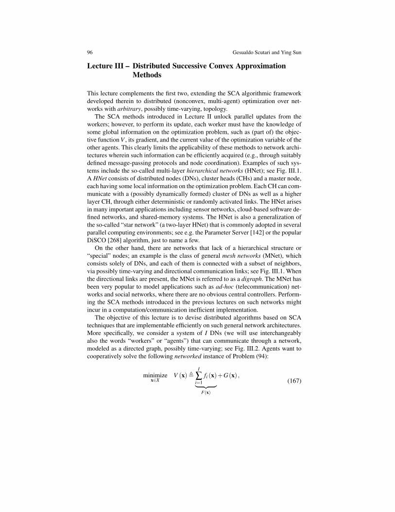
96 Gesualdo Scutari and Ying Sun
Lecture III – Distributed Successive Convex ApproximationMethods
This lecture complements the first two, extending the SCA algorithmic frameworkdeveloped therein to distributed (nonconvex, multi-agent) optimization over net-works with arbitrary, possibly time-varying, topology.
The SCA methods introduced in Lecture II unlock parallel updates from theworkers; however, to perform its update, each worker must have the knowledge ofsome global information on the optimization problem, such as (part of) the objec-tive function V , its gradient, and the current value of the optimization variable of theother agents. This clearly limits the applicability of these methods to network archi-tectures wherein such information can be efficiently acquired (e.g., through suitablydefined message-passing protocols and node coordination). Examples of such sys-tems include the so-called multi-layer hierarchical networks (HNet); see Fig. III.1.A HNet consists of distributed nodes (DNs), cluster heads (CHs) and a master node,each having some local information on the optimization problem. Each CH can com-municate with a (possibly dynamically formed) cluster of DNs as well as a higherlayer CH, through either deterministic or randomly activated links. The HNet arisesin many important applications including sensor networks, cloud-based software de-fined networks, and shared-memory systems. The HNet is also a generalization ofthe so-called “star network” (a two-layer HNet) that is commonly adopted in severalparallel computing environments; see e.g. the Parameter Server [142] or the popularDiSCO [268] algorithm, just to name a few.
On the other hand, there are networks that lack of a hierarchical structure or“special” nodes; an example is the class of general mesh networks (MNet), whichconsists solely of DNs, and each of them is connected with a subset of neighbors,via possibly time-varying and directional communication links; see Fig. III.1. Whenthe directional links are present, the MNet is referred to as a digraph. The MNet hasbeen very popular to model applications such as ad-hoc (telecommunication) net-works and social networks, where there are no obvious central controllers. Perform-ing the SCA methods introduced in the previous lectures on such networks mightincur in a computation/communication inefficient implementation.
The objective of this lecture is to devise distributed algorithms based on SCAtechniques that are implementable efficiently on such general network architectures.More specifically, we consider a system of I DNs (we will use interchangeablyalso the words “workers” or “agents”) that can communicate through a network,modeled as a directed graph, possibly time-varying; see Fig. III.2. Agents want tocooperatively solve the following networked instance of Problem (94):
minimizex∈X
V (x),I
∑i=1
fi (x)︸ ︷︷ ︸F(x)
+G(x) ,(167)
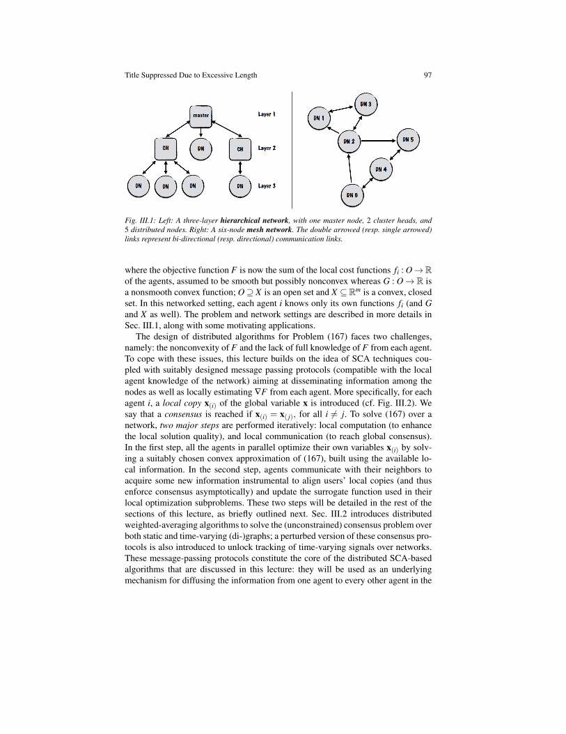
Title Suppressed Due to Excessive Length 97
Fig. III.1: Left: A three-layer hierarchical network, with one master node, 2 cluster heads, and5 distributed nodes. Right: A six-node mesh network. The double arrowed (resp. single arrowed)links represent bi-directional (resp. directional) communication links.
where the objective function F is now the sum of the local cost functions fi : O→Rof the agents, assumed to be smooth but possibly nonconvex whereas G : O→ R isa nonsmooth convex function; O⊇ X is an open set and X ⊆Rm is a convex, closedset. In this networked setting, each agent i knows only its own functions fi (and Gand X as well). The problem and network settings are described in more details inSec. III.1, along with some motivating applications.
The design of distributed algorithms for Problem (167) faces two challenges,namely: the nonconvexity of F and the lack of full knowledge of F from each agent.To cope with these issues, this lecture builds on the idea of SCA techniques cou-pled with suitably designed message passing protocols (compatible with the localagent knowledge of the network) aiming at disseminating information among thenodes as well as locally estimating ∇F from each agent. More specifically, for eachagent i, a local copy x(i) of the global variable x is introduced (cf. Fig. III.2). Wesay that a consensus is reached if x(i) = x( j), for all i 6= j. To solve (167) over anetwork, two major steps are performed iteratively: local computation (to enhancethe local solution quality), and local communication (to reach global consensus).In the first step, all the agents in parallel optimize their own variables x(i) by solv-ing a suitably chosen convex approximation of (167), built using the available lo-cal information. In the second step, agents communicate with their neighbors toacquire some new information instrumental to align users’ local copies (and thusenforce consensus asymptotically) and update the surrogate function used in theirlocal optimization subproblems. These two steps will be detailed in the rest of thesections of this lecture, as briefly outlined next. Sec. III.2 introduces distributedweighted-averaging algorithms to solve the (unconstrained) consensus problem overboth static and time-varying (di-)graphs; a perturbed version of these consensus pro-tocols is also introduced to unlock tracking of time-varying signals over networks.These message-passing protocols constitute the core of the distributed SCA-basedalgorithms that are discussed in this lecture: they will be used as an underlyingmechanism for diffusing the information from one agent to every other agent in the
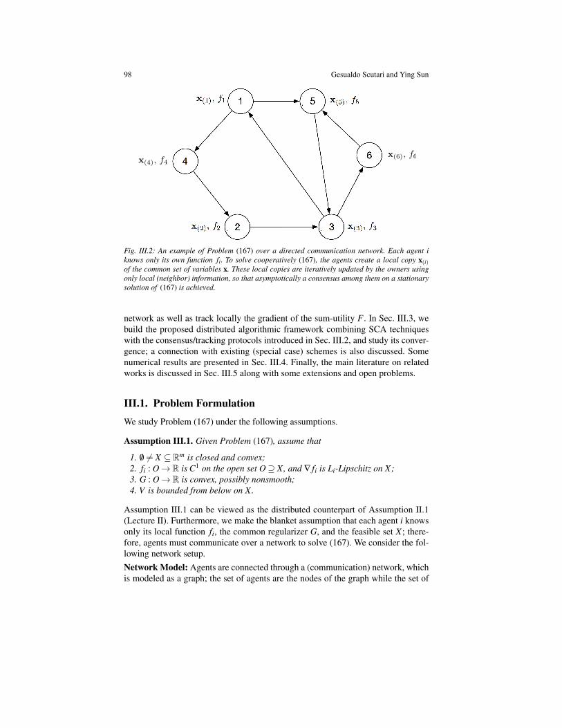
98 Gesualdo Scutari and Ying Sun
1
2 3
4
5
6x(4), f4
x(3), f3
x(5), f5
x(2), f2
x(6), f6
x(1), f1
Fig. III.2: An example of Problem (167) over a directed communication network. Each agent iknows only its own function fi. To solve cooperatively (167), the agents create a local copy x(i)of the common set of variables x. These local copies are iteratively updated by the owners usingonly local (neighbor) information, so that asymptotically a consensus among them on a stationarysolution of (167) is achieved.
network as well as track locally the gradient of the sum-utility F . In Sec. III.3, webuild the proposed distributed algorithmic framework combining SCA techniqueswith the consensus/tracking protocols introduced in Sec. III.2, and study its conver-gence; a connection with existing (special case) schemes is also discussed. Somenumerical results are presented in Sec. III.4. Finally, the main literature on relatedworks is discussed in Sec. III.5 along with some extensions and open problems.
III.1. Problem FormulationWe study Problem (167) under the following assumptions.
Assumption III.1. Given Problem (167), assume that
1. /0 6= X ⊆ Rm is closed and convex;2. fi : O→ R is C1 on the open set O⊇ X, and ∇ fi is Li-Lipschitz on X;3. G : O→ R is convex, possibly nonsmooth;4. V is bounded from below on X.
Assumption III.1 can be viewed as the distributed counterpart of Assumption II.1(Lecture II). Furthermore, we make the blanket assumption that each agent i knowsonly its local function fi, the common regularizer G, and the feasible set X ; there-fore, agents must communicate over a network to solve (167). We consider the fol-lowing network setup.Network Model: Agents are connected through a (communication) network, whichis modeled as a graph; the set of agents are the nodes of the graph while the set of

Title Suppressed Due to Excessive Length 99
edges represents the communication links. We will consider both static and time-varying graphs, as well as undirected and directed graphs. We will use the follow-ing notation: Gk =
(V,Ek
)denotes the directed graph that connects the agent at (the
discrete) time k, where V , 1, . . . , I is the set of nodes and Ek is the set of edges(agents’ communication links); we use (i, j)∈ Ek to indicate that the link is directedfrom node i to node j. The in-neighborhood of agent i at time k (including node iitself) is defined as Nin,k
i , j |( j, i) ∈ Ek∪i whereas its out-neighborhood (in-cluding node i itself) is defined as Nout,k
i , j | (i, j) ∈ Ek∪i. Of course, if thegraph is undirected, the set of in-neighbors and out-neighbors are identical. Theseneighbors capture the local view of the network from agent i at time k: At the timethe communication is performed, agent i can receive information from its currentin-neighbors and send information to its current out neighbors. Note that we implic-itly assumed that only inter-node (intermittent) communications between single-hopneighbors can be performed. The out-degree of agent i at time k is defined as thecardinality of Nout,k
i , and is denoted by dki , |Nout,k
i |. We will treat static and/orundirected graphs as special cases of the above time-varying directed setting.
An important aspect of graphs is their connectivity properties. An undirected(static) graph is connected if there is a path connecting every pair of two distinctnodes. A directed (static) graph is strongly connected if there is a directed path fromany node to any other node in the graph. For time-varying (di-)graphs we will invokethe following “long-term” connectivity property.
Assumption III.2 (B-strongly connectivity). The digraph sequence Gkk∈N+ isB-strongly connected, i.e., there exists an integer B > 0 (possibly unknown to theagents) such that the digraph with edge set ∪k+B−1
t=k Et is strongly connected, for allk ≥ 0.
Generally speaking, the above assumption permits strong connectivity to occur overa time window of length B: the graph obtained by taking the union of any B consecu-tive graphs is strongly connected. Intuitively, this let information propagate through-out the network. Assumption III.2 is standard and well-accepted in the literature.
III.1.1 Some motivating applicationsProblems in the form (167), under Assumptions III.1 and III.2, have found a widerange of applications in several areas, including network information processing,telecommunications, multi-agent control, and machine learning. In particular, theyare a key enabler of many nonconvex in-network “big data” analytic tasks, includingnonlinear least squares, dictionary learning, principal/canonical component anal-ysis, low-rank approximation, and matrix completion, just to name a few. Time-varying communications arise, for instance, in mobile wireless networks (e.g., ad-hoc networks) wherein nodes are mobile and/or communicate throughout fadingchannels. Moreover, since nodes generally transmit at different power and/or com-munication channels are not symmetric, directed links is a natural assumption. Someillustrative examples are briefly discussed next; see Sec. III.4 for more details andsome numerical results.

100 Gesualdo Scutari and Ying Sun
Example #1−(Sparse) empirical risk minimization: In Example #5 in Sec. II.1.1(Lecture II), we introduced the empirical risk minimization (ERM) problem, whichconsists in estimating a parameter x from a given data set DiI
i=1 by minimiz-ing the risk function F(x), ∑
Ii=1 `
(h(x,Di)
). Consider now the scenario where the
data set is not centrally available but split among I agents, connected through anetwork; agent i only owns the portion Di. All the agents want to collaborativelyestimate x, still minimizing F(x). This distributed counterpart of the ERM problemis an instance of (167), with fi(x) , `
(h(x,Di)
). Many distributed statistical learn-
ing problems fall under this umbrella. Examples include: the least squares prob-lem with fi(x) , ‖yi−Aix‖2, where Di , (yi,Ai); the sparse logistic regressionwith fi(x) , ∑
nij=1 log(1+ e−wi jyT
i jx), where Di , (wi j,yi j)nij=1, and their sparse
counterpart with suitable choices of the regularizer G(x) (cf. Table I.1 in Lecture I,Sec. I.4.1). Example #2−Sparse principal component analysis: Consider an m-dimensional data set din
i=1 with zero mean stored distributively among I agents,each agent i owns d j j∈Ni , where NiI
i=1 forms a partition of 1, . . . ,n. The prob-lem of sparse principal component analysis is to find a sparse direction x alongwhich the variance of the data points, measured by ∑
ni=1 ‖dT
i x‖2, is maximized.Construct the matrix Di ∈ R|Ni|×m by stacking d j j∈Ni row-wise, the problem canbe formulated as an instance of (167) with fi(x) , −‖Dix‖2, X , x |‖x‖2 ≤ 1,and G(x) being some sparsity promoting regularizer (cf. Table I.1 in Lecture I,Sec. I.4.1).Example #3−Target localization: Consider the problem of locating n targets usingmeasurements from I sensors, embedded in a network. Each sensor i knows its ownposition si and di t , the latter representing the squared Euclidean distance betweenthe target t and the node. Given the position xt of each target t, an error measurementof agent i is ei(xt), ∑
nt=1 pit (dit−‖xt − si‖2)2, where pit ∈ 0,1 is a given binary
variable taking value zero if the ith agent does not have any measurement related totarget t. The problem of estimating the locations xtn
t=1 can be thus formulated asan instance of (167), with x , xtn
t=1, fi(x) , ei(xt), and X , ∏nt=1 Xt , where Xt
characterizes the region where target t belongs to.
III.2. Preliminaries: Average Consensus and TrackingIn this section, we introduce some of the building blocks of the distributed algorith-mic framework that will be presented in Sec. III.3, namely: i) a consensus algorithmimplementable on undirected (Sec. III.2.1) and directed (Sec. III.2.2) time-varyinggraphs; ii) a dynamic consensus protocol to track the average of time-varying sig-nals over time-varying (directed) graphs (Sec. III.2.3); and iii) a perturbed consensusprotocol unifying and generalizing the schemes in i) and ii) (Sec. III.2.4).
III.2.1 Average consensus over undirected graphsThe consensus problem (also termed agreement problem) is one of the basic prob-lems arising in decentralized coordination and control. Here we are interested in theso-called average consensus problem, as introduced next.

Title Suppressed Due to Excessive Length 101
Consider a network of I agents, each of which having some initial (vector) vari-able ui ∈ Rm. The agents are interconnected over a (time-varying) network; thegraph modeling the network at time k is denoted by Gk (cf. Sec. III.1). Each agent icontrols a local variable x(i) that is updated at each iteration k using the informationof its immediate neighbors Nin,k
i ; we denote by xk(i) the value of x(i) at iteration k.
The average consensus problem consists in designing a distributed algorithm obey-ing the communication structure of each graph Gk, and enforcing
limk→∞‖xk
(i)− u‖= 0, ∀i = 1, . . . , I, with u,1I
I
∑i=1
ui.
One can construct a weighted-averaging protocol that solves the consensus prob-lem as follows. Let each x0
(i) = u0(i); given the iterate xk
(i), at time k+ 1, each agent
receives values xk( j) from its current (in-)neighbors, and updates its variable by set-
tingxk+1(i) = ∑
j∈Nin,ki
wki j xk
( j), (168)
where wki j are some positive weights, to be properly chosen. For a more compact
representation, we define the nonnegative weight-matrix1 Wk , (wki j)
Ii, j=1, whose
nonzero pattern is compliant with the topology of the graph Gk (in the sense ofAssumption III.3 below). Recall that the set of neighbors Nin,k
i contains also agent i(cf. Sec. III.1).
Assumption III.3. Given the graph sequence Gkk∈N+ , each matrix Wk, (wi j)Ii, j=1
satisfies:
1. wki j = 0, if ( j, i) /∈ Ek; and wk
i j ≥ κ , if ( j, i) ∈ Ek;2. wk
ii ≥ κ , for all i = 1, . . . , I;
for some given κ > 0.
Using Assumption III.3.1, we can write the consensus protocol (168) in the fol-lowing equivalent form
xk+1(i) =
I
∑j=1
wki j xk
( j). (169)
Note that (169) is compliant with the graph topology: the agents can only ex-change information (according to the direction of the edge) if there exists a commu-nication link between them. Also, Assumption III.3.2 states that each agent shouldinclude in the update (169) its own current information.
Convergence of xk(i)k∈N+ in (169) to the average u calls for the following extra
assumption.
Assumption III.4. Each Wk is doubly-stochastic, i.e., 1T Wk = 1T and Wk1 = 1.
1 Note that, for notational simplicity, here we use reverse links for the weight assignment, that is,each weight wi j is assigned to the directed edge ( j, i) ∈ Ek.

102 Gesualdo Scutari and Ying Sun
Table III.1: Examples of rules for doubly-stochastic weight matrices compliant to an undirectedgraph G = (V,E) (or a digraph admitting a double-stochastic matrix). In the Laplacian weightrule, λ is a positive constant and L is the Laplacian of the graph.
Rule Name Weight Expression
Metropolis-Hastings wi j =
1
maxdi,d j, if (i, j) ∈ E,
1−∑ j 6=i wki j, if i = j,
0, if (i, j) /∈ E and i 6= j;Laplacian W = I−λL, λ > 0
Maximum-degree wi j =
1/I, if (i, j) ∈ E,1− (di−1)/I, if i = j,0, if (i, j) /∈ E and i 6= j.
Assumption III.4 requires 1 being both the left and right eigenvector of Wk asso-ciated to the eigenvalue 1; intuitively, the column stochasticity plays the role ofpreserving the total sum of the x(i)’s (and thus the average) in the network while therow stochasticity locks consensus.
When the graphs Gk are undirected (or are directed and admits a compliantdoubly-stochastic matrix), several rules have been proposed in the literature to builda weight matrix satisfying Assumption III.3 and Assumption III.4. Examples in-clude the Laplacian weight rule [203]; the maximum degree weight, the Metropolis-Hastings, and the least-mean square consensus weight rules [258]. Table III.1 sum-marizes the aforementioned rules [202], where in the Laplacian weight rule, λ is apositive constant and L is the graph Laplacian, whose the i j-th entry Li j is definedas
Li j ,
di−1, if i = j;−1, if (i, j) ∈ E and i 6= j;0, otherwise;
(170)
where di is the degree of node i.Convergence of the average-consensus protocol (169) is stated in the next theo-
rem, whose proof is omitted because it is a special case of that of Theorem III.11(cf. Sec. III.2.4).
Theorem III.5. Let Gkk∈N+ be a sequence of graphs satisfying Assumption III.2.Consider the average-consensus protocol (169), where each Wkk∈N+ is chosenaccording to Assumptions III.3 and III.4. Then, the sequence xk , (xk
(i))Ii=1k∈N+
generated by (169) satisfies: for all k ∈ N+,
(a) Invariance of the average:
I
∑i=1
xk+1(i) =
I
∑i=1
xk(i) = · · ·=
I
∑i=1
x0(i); (171)
(b) Geometric decay of the consensus error:

Title Suppressed Due to Excessive Length 103∥∥∥∥∥xk(i)−
1I
I
∑j=1
xk( j)
∥∥∥∥∥≤ cu · (ρu)k · ‖x0‖, ∀i = 1, . . . , I, (172)
where x0 , (x0(i))
Ii=1, and cu > 0 and ρu ∈ (0,1) are constants defined as
cu ,2Iρu· 2(1+κ−(I−1)B)
1−κ(I−1)B and ρu ,(
1−κ(I−1)B
) 1(I−1)B
, (173)
with B and κ defined in Assumption III.2 and Assumption III.3, respectively.
In words, Theorem III.5 states that each xk(i) converges to the initial average
(1/I) · ∑Ii=1 x0
(i) at a geometric rate. Since x0(i) is initialized as x0
(i) , ui, each
xk(i)k∈N+ converges to u geometrically.
Remark III.6. While Theorem III.5 has been stated under Assumption III.4 (be-cause we are mainly interested in the convergence to the average u), it is importantto remark that the row-stochasticity of each Wk (rather than doubly-stochasticity) isenough for the sequence xkk∈N+ generated by the protocol (169) to geometricallyreach a consensus, that is, limk→∞ ‖xk
(i)− xk( j)‖ = 0, for all i, j = 1, . . . I and i 6= j.
However, the limit point of xkk∈N+ is no longer the average of the x0(i)’s.
III.2.2 Average consensus over directed graphs
A key assumption for the distributed protocol (169) to reach the average consensusis that each matrix Wk, compliant with the graph Gk, is doubly-stochastic.
While such constructions exist for networks with bi-directional (possibly time-varying) communication links, they become computationally prohibitive or infeasi-ble for networks with directed links, for several reasons. First of all, not all digraphsadmit a compliant (in the sense of Assumption III.3) doubly-stochastic weight ma-trix; some form of balancedness in the graph is needed [92], which limits the classof networks over which the consensus protocol (169) can be applied. Furthermore,conditions for a digraph to admit such a doubly-stochastic matrix are not easy tobe checked in practice; and, even when possible, constructing a doubly-stochasticweight matrix compliant to the digraph calls for computationally intense, generallycentralized, algorithms.
To solve the average consensus problem over digraphs that do not admit a doubly-stochastic matrix, a further assumption is needed [101] along with a modification ofthe protocol (169). Specifically, a standard assumption in the literature is that everyagent i knows its out-degree dk
i at each time k. This means that, while broadcastingits own message, every agent knows how many nodes will receive it. The problemof computing the out-degree using only local information has been considered ina number of works (see, e.g., [119, 243] and the references therein). Various algo-rithms have been proposed, mainly based on flooding, which, however, requires sig-nificant communication overhead and storage. A less demanding consensus-basedapproach can be found in [44].

104 Gesualdo Scutari and Ying Sun
Under the above assumption, the average consensus can be achieved on digraphsusing the so-called push-sum protocol [121]. Each agent i controls two local vari-ables, z(i) ∈ Rm and φi ∈ R, which are updated at each iteration k still using onlythe information of its immediate neighbors. The push-sum protocols reads: for alli = 1, . . . , I,
zk+1(i) =
I
∑j=1
aki j zk
( j),
φk+1(i) =
I
∑j=1
aki j φ
k( j),
(174)
where z(i) and φ(i) are initialized as z0(i) = ui and φ 0
(i) = 1, respectively; and the
coefficient aki j are defined as
aki j ,
1dk
j, if j ∈ Nin,k
i ,
0, otherwise.(175)
Note that the scheme (174) is a broadcast (i.e., one-way) communication protocol:each agent i broadcasts (“pushes out”) the values zk
( j)/dkj and φ k
( j)/dkj , which are re-
ceived by its out-neighbors; at the receiver side, every node aggregates the receivedinformation according to (174) (i.e., summing the pushed values, which explains thename “push-sum”).
Introducing the weight matrices Ak , (aki j)
Ii, j=1, it is easy to check that, for gen-
eral digraphs, Ak may no longer be row-stochastic (i.e., Ak1 = 1). This meansthat the z- and φ -updates in (174) do not reach a consensus. However, because1T Ak = 1T , the sums of the z- and φ -variables are preserved: at every iterationk ∈ N+,
I
∑i=1
zk+1(i) =
I
∑i=1
zk(i) = · · ·=
I
∑i=1
z0(i) =
I
∑i=1
ui,
I
∑i=1
φk+1(i) =
I
∑i=1
φk(i) = · · ·=
I
∑i=1
φ0(i) = I.
(176)
This implies that, if the iterates (zk(i)/φ k
(i))Ii=1 converge to a consensus (note that each
zk(i)/φ k
(i) is well-defined because the weights φ ki are all positive), then the consensus
value must be the average u, as shown next. Let c∞ be the consensus value, that is,limk→∞ zk
(i)/φ k(i) = c∞, for all i = 1, . . . , I. Then, it must be∥∥∥∥∥ I
∑i=1
ui− I · c∞
∥∥∥∥∥ (176)=
∥∥∥∥∥ I
∑i=1
(zk(i)−φ
k(i) · c∞
)∥∥∥∥∥≤ I ·I
∑i=1
∥∥∥zk(i)/φ
k(i)− c∞
∥∥∥−→k→∞
0, (177)
which shows that c∞ =(1/I) ·∑Ii=1 ui. Convergence of (zk
(i)/φ k(i))
Ii=1 to the consensus
is proved in [11, 121], which we refer to the interested reader.
Title Suppressed Due to Excessive Length 105
Here, we study instead an equivalent reformulation of the push-sum algorithm,as given in [211, 231], which is more suitable for the integration with optimiza-tion (cf. Sec. III.3). Eliminating the z-variables in (174), and considering arbitrarycolumn-stochastic weight matrices Ak , (ak
i j)Ii, j=1, compliant to the graph Gk [not
necessarily given by (175)], we have [211, 231]:
φk+1(i) =
I
∑j=1
aki j φ
k( j),
xk+1(i) =
1φ
k+1(i)
I
∑j=1
aki j φ
k( j) xk
( j),
(178)
where x0(i) is set to x0
(i) = ui/φ 0(i), for all i = 1, . . . , I; and φ 0
(i) are arbitrary positive
scalars such that ∑Ii=1 φ 0
(i) = I. For simplicity, hereafter, we tacitly set φ 0(i) = 1 (im-
plying x0(i) = ui), for all i = 1, . . . , I. Similarly to (174), in the protocol (178), every
agent i controls and updates the variables x(i) and φ(i), based on the informationφ k( j) and φ k
( j) xk( j) received from its current in-neighbors. We will refer to (178) as
condensed push-sum algorithm.Combining the weights ak
i j and the φ k(i) in the update of xk
(i) in a single coefficient
wki j ,
aki j φ k
( j)
∑Ij=1 ak
i j φ k( j)
, (179)
it is not difficult to check that the matrices Wk , (wki j)
Ii, j=1 are row-stochastic, that
is, Wk1 = 1, and compliant to Gk. This means that each xk+1(i) in (178) is updated
performing a convex combination of the variables (xk( j)) j∈Nin,k
i. This is a key prop-
erty that will be leveraged in Sec. III.3 to build a distributed optimization algorithmfor constrained optimization problems wherein the feasibility of the iterates is pre-served at each iteration. The above equivalent formulation also sheds light on therole of the φ -variables: they rebuild dynamically the missing row stochasticity ofthe weights ak
i j, thus enforcing the consensus on the x-variables.Since the following quantities are invariants of the dynamics (178) (recall that
Ak are column stochastic), that is, for all k ∈ N+,
I
∑i=1
φk+1(i) xk+1
(i) =I
∑i=1
φk(i) xk
(i) = · · ·=I
∑i=1
φ0(i) x0
(i) =I
∑i=1
ui,
I
∑i=1
φk+1(i) =
I
∑i=1
φk(i) = · · ·=
I
∑i=1
φ0(i) = I,
by a similar argument used in (177), one can show that, if the xk(i) are consensual–
limk→∞ xk(i) = x∞, for all i = 1, . . . , I–it must be x∞ = (1/I) ·∑I
i=1 ui. Convergence tothe consensus at geometric rate is stated in Theorem III.8 below, under the following
106 Gesualdo Scutari and Ying Sun
assumption on the weight matrices Ak (the proof of the theorem is omitted becauseit is a special case of that of Theorem III.11, cf. Sec. III.2.4).
Assumption III.7. Each Ak is compliant with Gk (i.e., it satisfies Assumption III.3)and it is column stochastic, i.e., 1T Ak = 1T .
Theorem III.8. Let Gkk∈N+ be a sequence of graphs satisfying Assumption III.2.Consider the condensed push-sum protocol (178), where each Akk∈N is chosenaccording to Assumption III.7. Then, the sequence xk , (xk
(i))Ii=1k∈N+ generated
by (178) satisfies: for all k ∈ N+,
(a) Invariance of the weighted-sum:
I
∑i=1
φk+1(i) xk+1
(i) =I
∑i=1
φk(i) xk
(i) = · · ·=I
∑i=1
φ0(i) x0
(i); (180)
(b) Geometric decay of the consensus error:∥∥∥∥∥xk(i)−
1I
I
∑j=1
φk( j) xk
( j)
∥∥∥∥∥≤ cd · (ρd)k · ‖x0‖, ∀i = 1, . . . , I, (181)
where x0 , (x0(i))
Ii=1, and cd > 0 and ρd ∈ (0,1) are defined as
cd ,2Iρ· 2(1+ κ
−(I−1)Bd )
1−κ(I−1)Bd
and ρd ,(
1− κ(I−1)Bd
) 1(I−1)B
,
and κd , κ2(I−1)B+1/I, with B and κ defined in Assumption III.2 and Assump-tion III.3, respectively.
Note that to reach consensus, the condensed push-sum protocol requires that theweight matrices Ak are column stochastic but not doubly-stochastic. Of course, onecan always use the classical push-sum weights as in (175), which is an exampleof rule satisfying Assumption III.7. Moreover, if the graph Gk is undirected or isdirected but admits a compliant doubly-stochastic matrix, one can also choose in(178) a doubly-stochastic Ak. In such a case, the φ -update in (178) indicates thatφ k(i) = 1, for all i = 1, . . . , I and k ∈N+. Therefore, (178) [and also (174)] reduces to
the plain consensus scheme (169).
III.2.3 Distributed tracking of time-varying signals’ average
In this section, we extend the condensed push-sum protocol to the case where thesignals ui are no longer constant but time-varying; the value of the signal at timek owned by agent i is denoted by uk
i . The goal becomes designing a distributedalgorithm obeying the communication structure of each graph Gk that tracks theaverage of (uk
i )Ii=1, i.e.,

Title Suppressed Due to Excessive Length 107
limk→∞‖xk
(i)− uk‖= 0, ∀i = 1, . . . , I, with uk ,1I
I
∑i=1
uki .
We first introduce the algorithm for undirected graphs (or directed ones that admita doubly-stochastic matrix); we then extend the scheme to the more general settingof arbitrary directed graphs.
Distributed tracking over undirected graphs
Consider a (possibly) time-varying network, modeled by a sequence of undirectedgraphs (or directed graphs admitting a doubly-stochastic matrix) Gkk∈N+ . As forthe average consensus problem, we let each agent i maintain and update a variablexk(i) that represents a local estimate of uk; we set x0
(i) , u0i . Since uk
i is time-varying,a direct application of the protocol (169), developed for the plain average consensusproblem, cannot work because it would drive all xk
(i) to converge to u0. Therefore,
we need to modify the vanilla scheme (169) to account for the variability of uki ’s.
We construct next the distributed tracking algorithm inductively, building on (169).Recall that, in the average consensus scheme (169), a key property to set the con-
sensus value to the average of the initial values x0(i) is the invariance of the average
∑Ii=1 xk
(i) throughout the dynamics (169):
I
∑i=1
xk+1(i) =
I
∑i=1
I
∑j=1
wki j xk
( j) =I
∑i=1
xk(i) = · · ·=
I
∑i=1
x0(i), (182)
which is met if the weight matrices Wk are column stochastic. The row-stochasticityof Wk enforces asymptotically a consensus. When it comes to solve the trackingproblem, it seems then natural to require such an invariance of the (time-varying)average, that is, ∑
Ii=1 xk
(i) = ∑Ii=1 uk
i , for all k ∈ N+, while enforcing a consensus on
xk(i)’s. Since x0
(i) , u0i we have ∑
Ii=1 x0
(i) , ∑Ii=1 u0
i . Suppose now that, at iteration k,
we have ∑Ii=1 xk
(i) = ∑Ii=1 uk
i . In order to satisfy ∑Ii=1 xk+1
(i) , ∑Ii=1 uk+1
i , it must be
I
∑i=1
xk+1(i) =
I
∑i=1
uk+1i
=I
∑i=1
uki +
I
∑i=1
(uk+1
i −uki
)(a)=
I
∑i=1
xk(i)+
I
∑i=1
(uk+1
i −uki
)(b)=
I
∑i=1
(I
∑j=1
wki j xk
( j)+(
uk+1i −uk
i
)),
(183)

108 Gesualdo Scutari and Ying Sun
where in (a) we used ∑Ii=1 xk
(i) = ∑Ii=1 uk
i ; and (b) follows from the column stochas-
ticity of Wk [cf. (182)]. This naturally suggests the following modification of theprotocol (169): for all i = 1, . . . , I,
xk+1(i) =
I
∑j=1
wki j xk
( j)+(
uk+1i −uk
i
), (184)
with x0(i) = u0
i , i = 1, . . . , I. Generally speaking, (184) has the following interpreta-
tion: by averaging neighbors’ information, the first term ∑Ij=1 wk
i j xk( j) aims at en-
forcing a consensus among the xk(i)’s while the second term is a perturbation that
bias the current sum ∑Ii=1 xk
(i) towards ∑Ii=1 uk
i . By (183) and a similar argument
as in (177), it is not difficult to check that if the xk(i) are consensual it must be
limk→∞ ‖xk(i)− uk‖ = 0, for all i = 1, . . . , I. Theorem III.10 proves this result (as a
special case of the tracking scheme over arbitrary directed graphs).
Distributed tracking over arbitrary directed graphs
Consider now the case of digraphs Gkk∈N+ with arbitrary topology. With theresults established in Sec. III.2.2, the tracking mechanism (184) can be naturallygeneralized to this more general setting by “perturbing” the condensed push-sumscheme (178) as follows: for i = 1, . . . , I,
φk+1(i) =
I
∑j=1
aki j φ
k( j),
xk+1(i) =
1φ
k+1(i)
I
∑j=1
aki j φ
k( j) xk
( j)+1
φk+1(i)
·(
uk+1i −uk
i
),
(185)
where x0(i) = u0
i /φ 0(i), i = 1, . . . , I; and (φ 0
(i))Ii=1 are arbitrary positive scalars such that
∑Ii=1 φ k
(i) = I. For simplicity, hereafter, we tacitly set φ 0(i) = 1, for all i= 1, . . . , I. Note
that, differently from (184), in (185), we have scaled the perturbation by (φ k+1(i) )−1
so that the weighted average is preserved, that is, ∑Ii=1 φ k
(i) xk(i) = ∑
Ii=1 uk
i , for allk ∈ N+.
Convergence of the tracking scheme (185) is stated in Theorem III.10 below,whose proof is omitted because is a special case of the more general result stated inTheorem III.11 (cf. Sec. III.2.4).
Assumption III.9. Let uki k∈N+ be such that
limk→∞‖uk+1
i −uki ‖= 0, ∀i = 1, . . . , I.
Theorem III.10. Let Gkk∈N+ be a sequence of graphs satisfying Assumption III.2.Consider the distributed tracking protocol (185), where each Ak is chosen according
Title Suppressed Due to Excessive Length 109
to Assumption III.7. Then, the sequence xk , (xk(i))
Ii=1k∈N+ generated by (185)
satisfies:
(a) Invariance of the weighted-sum:
I
∑i=1
φk(i) xk
(i) =I
∑i=1
uki , ∀k ∈ N+; (186)
(b) Asymptotic consensus: if, in addition, the sequence of signals (uki )
Ii=1k∈N+
satisfies Assumption III.9, then
limk→∞
∥∥∥xk(i)− uk
∥∥∥= 0, ∀i = 1, . . . , I. (187)
III.2.4 Perturbed condensed push-sum
In this section, we provide a unified proof of Theorems III.5, III.8, and III.10 byinterpreting the consensus and tracking schemes introduced in the previous sections[namely: (169), (178) and (185)] as special instances of the following perturbedcondensed push-sum protocol: for all i = 1, . . . , I, and k ∈ N+,
φk+1(i) =
I
∑j=1
aki j φ
k( j),
xk+1(i) =
1φ
k+1(i)
I
∑j=1
aki j φ
k( j) xk
( j)+εεεki ,
(188)
with given x0 , (x0(i))
Ii=1, and φ 0
(i) = 1, for all i = 1, . . . , I; where εεεki models a
perturbation locally injected into the system by agent i at iteration k. Clearly, theschemes (178) and (185) are special case of (188), obtained setting εεεk
i , 0 andεεεk
i , (φ k+1(i) )−1(uk+1
i −uki ), respectively. Furthermore, if the matrices Ak are doubly-
stochastic, we obtain as special cases the schemes (169) and (184), respectively.Convergence of the scheme (188) is given in the theorem below.
Theorem III.11. Let Gkk∈N+ be a sequence of graphs satisfying Assumption III.2.Consider the perturbed condensed push-sum protocol (188), where each Ak is cho-sen according to Assumption III.7. Then, the sequences xk , (xk
(i))Ii=1k∈N+ and
φφφ k , (φ k(i))
Ii=1k∈N+ generated by (188) satisfy:
(a) Bounded φφφ kk∈N+:
φlb , infk∈N+
min1≤i≤I
φk(i) ≥ κ
2(I−1)B,
φub , supk∈N+
max1≤i≤I
φk(i) ≤ I−κ
2(I−1)B;(189)
110 Gesualdo Scutari and Ying Sun
(b) Bounded consensus error: for all k ∈ N+,∥∥∥∥∥xk(i)−
1I
I
∑j=1
φk( j) xk
( j)
∥∥∥∥∥≤ c ·((ρ)k ‖x0‖+
k−1
∑t=0
(ρ)k−1−t ‖εεε t‖), ∀i = i, . . . , I,
(190)where εεεk , (εεεk
i )Ii=1, and c > 0 and ρ ∈ (0,1) are constants defined as
c,2Iρ· 2(1+ κ−(I−1)B)
1− κ(I−1)B and ρ ,(
1− κ(I−1)B
) 1(I−1)B
,
with κ , κ ·(φlb/φub
), and B and κ defined in Assumption III.2 and Assump-
tion III.3, respectively.
Proof. See Sec. III.2.5.
DiscussionLet us apply now Theorem III.11 to study the impact on the consensus value of thefollowing three different perturbation errors:
1) Error free: εεεki = 0, for all i = 1, . . . , I, and k ∈ N+;
2) Vanishing error: limk→∞ ‖εεεki ‖= 0, for all i = 1, . . . , I, and k ∈ N+;
3) Bounded error: There exists a constant 0 ≤M <+∞ such that ‖εεεki ‖ ≤M, for
all i = 1, . . . , I, and k ∈ N+.
Case 1: Error free. Since εεεki = 0, i = 1, . . . , I, the perturbed consensus protocol
(188) reduces to the condensed push-sum consensus scheme (178). According toTheorem III.11, each xk
(i) converges to the weighted average (1/I) ·∑Ii=1 φ k
(i)xk(i) ge-
ometrically. Since (1/I) ·∑Ii=1 φ k
(i)xk(i) = (1/I) ·∑I
i=1 φ 0(i)x
0(i) = u, for all k ∈N+, each
‖xk(i)− u‖ vanishes geometrically, which proves Theorem III.8.
If, in addition, the weighted matrices Ak are also row-stochastic (and thus doubly-stochastic), we have φ k
(i) = 1, for all k ∈ N+. Therefore, (188) reduces to the vanillaaverage consensus protocol (169); and in TheoremIII.11 we have κ = κ , whichproves Theorem III.5 as a special case.
Case 2: Vanishing error. To study the consensus value in this setting, we need thefollowing lemma on the convergence of product of sequences.
Lemma III.12 ([148, Lemma 7]). Let 0 < λ < 1, and let β kk∈N+ and νkk∈N+
be two positive scalar sequences. Then, the following hold:
(a) If limk→∞
β k = 0, then
limk→∞
k
∑t=1
(λ )k−tβ
t = 0.
Title Suppressed Due to Excessive Length 111
(b) If∞
∑k=1
(β k)2 < ∞ and∞
∑k=1
(νk)2 < ∞, then
1) limk→∞
k∑
t=1
t∑
l=1(λ )t−l (β l)2 < ∞;
2) limk→∞
k∑
t=1
t∑
l=1(λ )t−l β t ν l < ∞.
Consider (190): Since ρ ∈ (0,1), invoking Lemma III.12(a) and limk→∞ ‖εεεk‖= 0,we have
limk→∞
k−1
∑t=0
(ρ)k−1−t ‖εεε t‖= 0; (191)
hence limk→∞ ‖xk(i)− (1/I) ·∑I
j=1 φ k( j)x
k( j)‖ = 0 Note that, in this case, the rate of
convergence to the weighted average may not be geometric.Consider, as special case, the tracking algorithm (185). i.e., set in (188) εεεk
i =
(φ k+1(i) )−1(uk+1
i −uki ). We have (1/I)·∑I
i=1 φ k(i)x
k(i)= uk, which proves Theorem III.10.
Case 3: Bounded error. Since ‖εεεki ‖ ≤M, i = 1, . . . , I, the consensus error in (190)
can be bounded as∥∥∥∥∥xk(i)−
1I
I
∑j=1
φk( j)x
k( j)
∥∥∥∥∥≤c
((ρ)k‖x0‖+M ·
k−1
∑t=0
(ρ)k−1−t
)
≤c((ρ)k‖x0‖+M · 1− (ρ)k−1
1−ρ
).
(192)
III.2.5 Proof of Theorem III.11
We prove now Theorem III.11, following the analysis in [211]. We first introducesome intermediate results and useful notation.
PreliminariesIt is convenient to rewrite the perturbed consensus protocol (188) in a more com-pact form. To do so, let us introduce the following notation: given the matrix Ak
compliant to the graph Gk (cf. Assumption III.3) and Wk defined in (179), let
xk , [xkT(1), . . . ,x
kT(I)]
T , (193)
εεεk , [εεεkT
1 , . . . ,εεεkTI ]T , (194)
φφφk , [φ k
(1), . . . ,φk(I)]
T , (195)
ΦΦΦk , Diag(φφφ k), (196)
ΦΦΦk,ΦΦΦ
k⊗ Im, (197)

112 Gesualdo Scutari and Ying Sun
Ak , Ak⊗ Im, (198)
Wk ,Wk⊗ Im, (199)
where Diag(•) denotes a diagonal matrix whose diagonal entries are the elementsof the vector argument. Under the column stochasticity of Ak (Assumption III.7),it is not difficult to check that the following relationship exists between Wk and Ak
(and Wk and Ak):
Wk =(ΦΦΦ
k+1)−1 AkΦΦΦ
k and Wk =(ΦΦΦ
k+1)−1 AkΦΦΦ
k. (200)
Using the above notation, the perturbed consensus protocol (188) can be rewrit-ten in matrix form as
φφφk+1 = Ak
φφφk and xk+1 = Wk xk +εεε
k. (201)
To study the dynamics of the consensus error in (201), let us introduce the matrixproducts: given k, t ∈ N+, with k ≥ t,
Ak:t ,
AkAk−1 · · ·At , if k > t ≥ 0,Ak, if k = t ≥ 0,
(202)
Wk:t ,
WkWk−1 · · ·Wt , if k > t ≥ 0,Wk, if k = t ≥ 0,
(203)
and
Ak:t , Ak:t ⊗ Im, (204)
Wk:t ,Wk:t ⊗ Im. (205)
Define the weight-averaging matrix as
Jφφφ k ,
1I
(1(φφφφφφφφφ k)T
)⊗ Im, (206)
so that
Jφφφ k xk = 1⊗ 1
I
I
∑i=1
φk(i)x
k(i),
i.e., Jφφφ k xk computes the average of xk
(i) weighted by (φ k(i))
Ii=1 and stacks it I times
in a column vector. Under the column stochasticity of Ak (Assumption III.7), it isnot difficult to check that the following property holds between J
φφφ k and Wk:t : for allk, t ∈ N+, with k ≥ t,
Jφφφ k+1 Wk:t = Jφφφ t = Wk:t Jφφφ t . (207)
Convergence of the perturbed consensus protocol boils down to studying the dy-namics of ‖Wk:t −Jφφφ t‖ (this will be more clear in the next subsection). The follow-

Title Suppressed Due to Excessive Length 113
ing lemma shows that, in the setting of Theorem III.11, Wk:t converges geometri-cally to Jφφφ t ; the proof of the lemma is omitted and can be found in [211, Lemma 2].
Lemma III.13. Let Gkk∈N+ be a sequence of graphs satisfying Assumption III.2;let Akk∈N+ be a sequence of weight matrices satisfying Assumption III.7; and letWkk∈N+ be the sequence of (row-stochastic) matrices with Wk related to Ak by(200). Then, the following holds: for all k, t ∈ N+, with k ≥ t,∥∥∥Wk:t −Jφφφ t
∥∥∥2≤ c · (ρ)k−t+1, (208)
where c > 0 and ρ ∈ (0,1) are defined in Theorem III.11.
Proof of Theorem III.11We are now ready to prove the theorem. We start rewriting the dynamics of theconsensus error xk−J
φφφ k xk in a form that permits the application of Lemma III.13.Applying the x-update in (201) recursively, we have
xk =Wk−1xk−1 +εεεk−1
=Wk−1(
Wk−2xk−2 +εεεk−2)+εεε
k−1
= · · ·= Wk−1:0 x0 +k−1
∑t=1
Wk−1:tεεε
t−1 +εεεk−1.
(209)
Therefore, the weighted average Jφφφ k xk can be written as
Jφφφ k xk (209)
= Jφφφ k Wk−1:0 x0 +J
φφφ k
k−1
∑t=1
Wk−1:tεεε
t−1 +Jφφφ k εεε
k−1
(207)= Jφφφ0 x0 +
k−1
∑t=1
Jφφφ t εεεt−1 +J
φφφ k εεεk−1.
(210)
Using (209) and (210) and Lemma III.13, the consensus error can be bounded as∥∥∥xk−Jφφφ k xk
∥∥∥=
∥∥∥∥∥(Wk−1:0−Jφφφ0
)x0 +
k−1
∑t=1
(Wk−1:t −Jφφφ t
)εεε
t−1 +(
I−Jφφφ k
)εεε
k−1
∥∥∥∥∥(208)≤ c · (ρ)k‖x0‖+ c ·
k−1
∑t=1
(ρ)k−t ‖εεε t−1‖+∥∥∥I−J
φφφ k
∥∥∥2︸ ︷︷ ︸
≤√
2 I
‖εεεk−1‖
≤ c ·((ρ)k‖x0‖+
k−1
∑t=0
(ρ)k−t−1 ‖εεε t‖),
(211)
114 Gesualdo Scutari and Ying Sun
where in the last inequality we used c >√
2 I. The inequality ‖I−Jφφφ k‖2 ≤
√2 I can
be proved as follows. Let z ∈ RI·m be an arbitrary vector; partition z as z = (zi)Ii=1,
with each zi ∈ Rm. Then,∥∥∥z−Jφφφ k z∥∥∥≤ ‖z−J1 z‖+
∥∥∥J1z−Jφφφ k z∥∥∥ (a)≤ ‖z‖+
√I
I
∥∥∥∥∥ I
∑i=1
zi−I
∑i=1
φki zi
∥∥∥∥∥≤ ‖z‖+
√I
I
√I2− I ‖z‖ ≤
√2 I ‖z‖ ,
where in (a) we used ‖I−J1‖= 1 (note that I−J1 is a Toeplitz matrix, with diagonalentries equal to 1− 1/I and off-diagonal entries all equal to −1/I; therefore, itseigenspectrum is given by 0,1, . . . ,1).
The inequality (211) proves the theorem.
III.3. Distributed SCA over Time-Varying Digraphs
We are now ready to introduce the proposed distributed algorithmic framework tosolve Problem (167), which combines SCA techniques (introduced in the previouslectures) with the consensus/tracking protocols described in Sec. III.2. We considerthe optimization over time-varying (B-strongly connected) digraphs (cf. Assump-tion III.2); distributed algorithms for undirected or time invariant networks can beobtained as special cases.
As already anticipated, each agent i maintains and updates iteratively a localcopy x(i) of the global variable x, along with an auxiliary variable y(i) ∈ Rm, whosegoal is to track locally the average of the gradients (1/I) ·∑I
i=1 ∇ fi (the importanceof this extra variable will be clarified shortly), an information that is not availableat the agent’s side; let xk
(i) and yk(i) denote the values of x(i) and y(i) at iteration k,
respectively. To update these variables, two major steps are performed iteratively,namely:
Step 1–Local SCA (optimization): Given xk(i) and yk
(i), each agent i solves a con-vexification of Problem (167), wherein V is replaced by a suitably chosenstrongly convex surrogate, which is built using only the available local infor-mation xk
(i) and yk(i);
Step 2–Communication: All the agents broadcast the solutions computed in Step1, and update their own variables xk
(i) → xk+1(i) and yk
(i) → yk+1(i) , based on the
information received from their neighbors.
The two steps above need to be designed so that: i) all the xk(i) will be asymptotically
consensual, that is, limk→∞ ‖xk(i)− (1/I) ·∑I
j=1 xk( j)‖= 0, for all i; and ii) every limit
point of (1/I) ·∑Ij=1 xk
( j) is a stationary solution of Problem (167). We describe nextthe above two steps in detail.Step 1: Local SCA (optimization). Each agent i faces two issues to solve Prob-lem (167), namely: fi is not convex and ∑ j 6=i f j is not known. To cope with the first
Title Suppressed Due to Excessive Length 115
issue, we leverage the SCA techniques introduced in the previous lectures. Morespecifically, at iteration k, agent i solves a convexification of V in (167) having thefollowing form
xi(xk(i)
), argmin
x(i)∈XFi(x(i) | xk
(i)
)+G
(x(i)), (212)
where Fi : O×O→ R is a suitably chosen surrogate of F . To guarantee that a fixedpoint of xi(•) is a stationary solution of (167), a naive application of the SCA theorydeveloped in Lecture II, would call Fi to satisfy the following gradient consistencycondition (cf. Assumption II.2, Sec. II.2): Fi is C1 on O and
∇Fi(xk(i) | xk
(i)
)= ∇F
(xk(i)
)= ∇ fi
(xk(i)
)+∑
j 6=i∇ f j(xk
(i)), k ∈ N+. (213)
For example, a surrogate function satisfying the above condition would be:
Fi(x(i) |xk
(i)
)= fi
(x(i) | xk
(i)
)+
(∑j 6=i
∇ f j(xk(i)
))T (x(i)−xk
(i)
), (214)
where fi(• | xk(i)) : O→R is a strongly convex surrogate of fi on X , consistent to fi,
in the following sense (cf. Assumption II.2).
Assumption III.14. Each function fi : O×O→R satisfies the following conditions:
1. fi (•|x) is τi-strongly convex on X, for all x ∈ X;
2. fi (•|x) is C1 on O and ∇ fi (x |x) = ∇ fi (x), for all x ∈ X;
3. ∇ fi (x |•) is Li-Lipschitz on X, for all x ∈ X.
Unfortunately, the surrogate function in (214) cannot be used by agent i, becauseof the lack of knowledge of ∑ j 6=i ∇ f j(xk
(i)); hence a gradient consistency conditionin the form (213) cannot be enforced in such a distributed setting.
To cope with this issue, the idea, first proposed in [148] and further developed in[211], is to replace ∑ j 6=i ∇ f j(xk
(i)) in (214) [and in (213)] with a local, asymptoticallyconsistent, approximation, so that condition (213) will be satisfied in the limit, ask→ ∞. This can be accomplished, e.g., using the following surrogate function:
Fi
(x(i) |xk
(i),yk(i)
)= fi
(x(i) |xk
(i)
)+(
I ·yk(i)−∇ fi(xk
(i)))T (
x(i)−xk(i)
), (215)
where fi is defined as in (214); and yk(i) in (215) is an auxiliary variable controlled by
agent i, aiming at tracking locally the average of the gradients (1/I) ·∑Ij=1 ∇ f j(xk
(i)),
that is, limk→∞ ‖yk(i)−(1/I) ·∑I
j=1 ∇ f j(xk(i))‖= 0. This explains the role of the linear
term in (215): under the claimed tracking property of yk(i), we have
limk→∞
∥∥∥∥∥(I ·yk(i)−∇ fi(xk
(i)))−∑
j 6=i∇ f j(xk
(i))
∥∥∥∥∥= 0, (216)
116 Gesualdo Scutari and Ying Sun
which would guarantee that the gradient consistency condition (213), with nowFi(• | xk
(i)) replaced by Fi(•|xk(i),y
k(i)) in (215), will be asymptotically satisfied, that
is,limk→∞
∥∥∥∇Fi(xk(i) |xk
(i),yk(i))−∇F(xk
(i))∥∥∥= 0.
As it will be shown later, this relaxed condition is in fact enough to prove that,if convergence and consensus are asymptotically achieved, the limit point of allthe local variables xk
(i) is a stationary solution of Problem (167). Leveraging thedistributed tracking protocol (185) (cf. Sec. III.2.3), in Step 2 below, we show howto devise an update for the yk
(i) variables that uses only local information and suchthat (216) asymptotically holds.
Using Fi(•|xk(i),y
k(i)) defined in (215), the local optimization step performing by
each agent i consists then in solving the following strongly convex problem:
xki , argmin
x(i)∈XFi
(x(i) |xk
(i),yk(i)
)+G
(x(i)), (217)
followed by the step-size update
xk+1/2(i) = xk
(i)+ γk(
xki −xk
(i)
), (218)
where γk ∈ (0,1] is the step-size, to be properly chosen.
Step 2–Communication. Given xk+1/2(i) and yk
(i), each agent i communicates with itscurrent neighbors in order to achieve asymptotic consensus on x(i)’s as well as track(1/I) ·∑I
j=1 ∇ f j(xk(i)) by yk
(i). Both goals can be accomplished using (two instancesof) the condensed perturbed push-sum protocol (188), introduced in Sec. III.2.4.
More specifically, after obtaining xk+1/2( j) from its neighbors, each agent i updates
its own local estimate x(i) employing:
φk+1(i) =
I
∑j=1
aki j φ
k( j); (219)
xk+1(i) =
1φ
k+1(i)
I
∑j=1
aki j φ
k( j) xk+1/2
( j) , (220)
where the weights Ak , (aki j)
Ii=1 are chosen according to Assumption III.7; and the
φ k(i) variables are initialized to φ 0
(i) = 1. This update can be clearly implemented
locally: All agents i) send their local variables φ k( j) and φ k
( j) xk+1/2( j) to their out-
neighbors; and ii) linearly combine with coefficients aki j the information coming
from their in-neighbors.A local update for the yk
(i) variable aiming at tracking (1/I) ·∑Ij=1 ∇ f j(xk
(i)) can bereadily obtained invoking the distributed tracking protocol (185), and setting therein
Title Suppressed Due to Excessive Length 117
uki , ∇ fi(xk
(i)). This leads to
yk+1(i) =
1φ
k+1(i)
I
∑j=1
aki j φ
k( j) yk
( j)+1
φk+1(i)
(∇ fi(xk+1(i)
)−∇ fi
(xk(i)
)), (221)
where φk+1(i) is defined in (219), and y0
(i) =∇ fi(x0(i)). Note that, as for xk+1
(i) , the update
of yk(i) is performed by agent i using only the information coming from its neighbors,
with the same signaling as for (219)-(220).The described distributed SCA method (Step 1 and Step 2) is summarized in
Algorithm 10, and termed distributed Successive cONvex Approximation algorithmover Time-varying digrAphs (SONATA).
Algorithm 10: SCA over Time-varying Digraphs (SONATA)
Data : x0(i) ∈ X , φ 0
(i) = 1, y0(i) = ∇ fi(x0
(i)), for all i = 1, . . . , I; γk ∈ (0,1]k∈N+ .Set k = 0.
(S.1) : If xk satisfies a termination criterion: STOP;(S.2) : Local SCA. Each agent i computes
xki , argmin
x(i)∈Xfi
(x(i) |xk
(i)
)+(
I ·yk(i)−∇ fi(xk
(i)))T (
x(i)−xk(i)
)+G
(x(i)),
xk+1/2(i) = xk
(i)+ γk(
xki −xk
(i)
);
(S.3) : Averaging and gradient tracking.Each agent i sends out its local variables φ k
(i), xk+1/2(i) and yk
(i), and receives
φ k( j), xk+1/2
( j) and yk( j), with j ∈ Nin,k
i \i. Then, it updates:
φk+1(i) =
I
∑j=1
aki j φ
k( j),
xk+1(i) =
1φ
k+1(i)
I
∑j=1
aki j φ
k( j) xk+1/2
( j) ,
yk+1(i) =
1φ
k+1(i)
I
∑j=1
aki j φ
k( j) yk
( j)+1
φk+1(i)
(∇ fi(xk+1(i)
)−∇ fi
(xk(i)
));
(S.4) : k← k+1, and go to (S.1).
Convergence of Algorithm 10 is stated in Theorem III.16 below. We first intro-duce a standard condition on the steps-size γk and a proper merit function assessingthe convergence of the algorithm.

118 Gesualdo Scutari and Ying Sun
Assumption III.15. The step-size γk ∈ (0,1] satisfies the standard diminishing rule:limk→∞ γk = 0 and ∑
∞k=0 γk =+∞.
Given xk , (xk(i))
Ii=1k∈N+ generated by Algorithm 10, convergence of the algo-
rithm is stated measuring the distance of the average sequence xk , (1/I) ·∑Ii=1 xk
(i)from optimality and well as the consensus disagreement among the local variablesxk(i)’s. More specifically, let us introduce the following function as a measure of
optimality:
J(xk),
∥∥∥∥∥xk− argminy∈X
∇F(xk)T (y− xk)+
12‖y− xk‖2
2 +G(y)∥∥∥∥∥ . (222)
Note that J is a valid measure of stationarity because it is continuous and J(x∞) = 0if and only if x∞ is a d-stationary solution of Problem (167). The consensus dis-agreement at iteration k is defined as
D(xk), ‖xk−1I⊗ xk‖2.
Note that D is equal to 0 if and only if all the xk(i)’s are consensual. We combine the
metrics J and D in a single merit function, defined as
M(xk),max
J(xk)2, D(xk)2,which captures the progresses of the algorithm towards optimality and consensus.
We are now ready to state the main convergence results for Algorithm 10.
Theorem III.16. Consider Problem (167) under Assumption III.1; and let Gkk∈N+
be a sequence of graphs satisfying Assumption III.2. Let xk , (xk(i))
Ii=1k∈N+ be the
sequence generated by Algorithm 10 under Assumptions III.7 and III.14; and letxk = (1/I) ·∑I
i=1 xk(i) be the average sequence. Furthermore, suppose that either one
of the following is satisfied.
(a) (diminishing step-size): The step-size γk satisfies Assumption III.15;(b) (constant step-size): The step-size γk is fixed–γk = γ , for all k ∈ N+–
and it is sufficiently small (see [211, Theorem 5] for the specific expression ofthe upper bound on γ).
Then, there holdslimk→∞
M(xk) = 0. (223)
Proof. See Sec. III.3.2.
Theorem III.17 below provides an upper bound on the number of iterationsneeded to decrease MU (xk) below a given accuracy ε > 0; we omit the proof andrefer to [211, Theorem 6] for more details.
Theorem III.17. Consider Problem (167) and Algorithm 10 in the setting of Theo-rem III.16. Given ε > 0, let Tε be the first iteration k such that M(xk)≤ ε .
Title Suppressed Due to Excessive Length 119
(a) (diminishing step-size): Suppose that the step-size γk satisfies As-sumption III.15. Then,
Tε ≤ inf
k ∈ N+ :
k
∑t=0
γt ≥ B0
ε
,
where B0 > 0 is a constant independent on ε [211];(b) (constant step-size): Suppose that the step-size γk is fixed, γk = γ , for
all k ∈ N+. Then, there exists a sufficiently small γ ∈ (0,1]–independent of ε
(see [211, Theorem 6] for the specific expression of γ)–such that, if γ ∈ (0, γ],then it holds
Tε = O(1
ε
).
Discussion and generalizations
On the convergence: Stating convergence for constrained (nonsmooth) optimiza-tion problems in the form (167), Theorem III.16 and Theorems III.17 (proved in ourwork [211]) significantly enlarge the class of convex and nonconvex problems whichdistributed algorithms can be applied to with convergence guarantees. We remarkthat convergence is established without requiring that the (sub)gradients of F or Gis bounded; this is a major improvement with respect to current distributed methodsfor nonconvex problems [20, 148, 232, 245] and nonsmooth convex ones [168].
We remark that convergence (as stated in the above theorems) can also be es-tablished weakening the assumption on the strongly convexity of the surrogatesfi (Assumption III.14) to just convexity, as long as the feasible set X is compact.Also, with mild additional assumptions on G–see Lecture II–convergence can bealso proved in the case wherein agents solve their subproblems (217) inexactly.ATC- versus CAA updates. As a final remark, we note that variants of SONATAwherein the order of the consensus, tracking, and local updates are differently com-bined, are still convergent, in the sense of Theorems III.16 and III.17. We brieflyelaborate on this issue next.
Using a jargon well established in the literature [202], the update of the x-variables in Step 3 of Algorithm 10 is in the form of so-called Adapt-Then-Combine(ATC) strategy: eliminating the intermediate variable xk+1/2
(i) , each xki follows the
dynamic
xk+1(i) =
1φ
k+1(i)
I
∑j=1
aki j φ
k( j)
(xk( j)+ γ
k(
xkj−xk
( j)
)). (224)
The name ATC comes from the form of (224): each agent i first “adapts” its localcopy xk
(i) moving along the direction xki −xk
(i), that is, xk(i)→ xk
(i)+γk (xki −xk
(i)); andthen it “combines” its new update with that of its in-neighbors.
As an alternative to (224), one can employ the so-called Combine-And-Adapt(CAA) update (also termed “consensus strategy” in [202]), which reads
120 Gesualdo Scutari and Ying Sun
xk+1(i) =
1φ
k+1(i)
I
∑j=1
aki j φ
k( j) xk
( j)+φ k(i)
φk+1(i)
· γk(
xki −xk
(i)
). (225)
According to this protocol, each agent i first “combines” (by weighted-averaging) itscurrent xk
(i) with those of its neighbors, and then “adapt” the resulting update moving
along the direction xki − xk
(i). Note that, when dealing with constraint optimization,the CAA update in general does not preserve the feasibility of the iterates while theATC protocol deos.
The ATC and CAA protocols can be interchangeably used also in the update ofthe tracking variables yk
(i) in Step 3 of SONATA. While the y-update as stated in thealgorithm [cf. (221)] is in the CAA form, one can also use the ATC-based update,which reads
yk+1(i) =
1φ
k+1(i)
I
∑j=1
aki j
(φ
k( j)y
k( j)+∇ f j
(xk+1( j)
)−∇ f j
(xk( j)
)).
One can show that the above versions of SONATA are all convergent.
III.3.1 SONATA (Algorithm 10) and special cases
The SONATA framework represents a gamut of algorithms, each of them corre-sponding to a specific choice of the surrogate functions, step-size, and weight ma-trices. In this section, we focus on recent proposals in the literature that built on theidea of distributed gradient tracking [69, 70, 148, 170, 190, 257, 259], and we showthat all of them are in fact special cases of SONATA. A more detailed analysis ofthe state of the art can be found in Sec. III.5.
The idea of tracking the gradient averages through the use of consensus cou-pled with distributed optimization was independently introduced in the NEXT &SONATA framework [69, 70, 148] & [211, 231] for the general class of (convex)constrained nonsmooth nonconvex problems (167) and in [259] for the special caseof strongly convex unconstrained smooth optimization. The algorithmic frameworkin [69, 70, 148] is applicable to optimization problems over time-varying graphs,but requires the use of doubly stochastic matrices. This assumption was removed inSONATA [211, 231] by using column-stochastic matrices, which are more generalthan the degree-based column-stochastic matrices of distributed push-sum-basedmethods. The scheme in [259] is implementable only over undirected fixed graphs.A convergence rate analysis of the scheme in [259] in the case of strongly convexsmooth unconstrained optimization problems was later developed in [170, 190] forundirected graphs and in [170] for time-varying directed graphs. Complexity resultsfor NEXT and SONATA for (strongly) convex and nonconvex constrained optimiza-tion problems over (time-varying) digraphs can be found in [211, 229]; differentlyfrom [170, 190], the analysis in [211, 229] applies to general surrogate functions(satisfying Assumption III.14).
We establish next a formal connection between SONATA and all these schemes.

Title Suppressed Due to Excessive Length 121
Preliminaries
Since all the aforementioned works but [69, 70, 148] are applicable only to the spe-cial instance of Problem (167) wherein X =Rm (unconstrained), G= 0 (only smoothobjectives), and F is strongly convex, throughout this section, for a fair comparison,we only consider this setting. We begin customizing Algorithm 10 to this specialinstance of (167) as follows. Choose each surrogate function fi in (215) as
fi(x(i) |xk(i)) = fi(xk
(i))+∇ fi(xk(i))
T (x(i)−xk(i))+
I2
∥∥∥x(i)−xk(i)
∥∥∥2.
This leads to the following closed form expression for xki in (217) (recall that X =
Rm and G = 0):
xki = argmin
xi
(I ·yk
(i)
)>(x(i)−xk
(i)
)+
I2
∥∥∥x(i)−xk(i)
∥∥∥2
= xk(i)−yk
(i).
(226)
Define now gki ,∇ fi(xk
(i)), gk = [gk T1 , . . . ,yk T
I ]T , and yk = [yk T(1), . . . ,g
k T(I) ]
T ; and recall
the definitions of φφφ k, ΦΦΦk, Ak, Wk and Wk introduced in Sec. III.2.5. Using (226),Algorithm 10 under the ATC or CAA updates can be rewritten in vector/matrix formas: for all k ∈ N+,
φφφk+1 = Ak
φφφk,
Wk = (ΦΦΦk+1)−1AkΦΦΦ
k,
xk+1 =
Wk(xk− γk yk
), if ATC is employed;
Wkxk− γk (ΦΦΦk+1
)−1ΦΦΦkyk, if CAA is employed;
(227)
yk+1 =
Wk
(yk +(ΦΦΦ
k)−1(gk+1−gk)
), if ATC is employed;
Wk yk +(ΦΦΦk+1
)−1(gk+1−gk
), if CAA is employed;
which we will refer to as ATC/CAA-SONATA-L (L stands for “linearized”).In the special case where all Ak are doubly-stochastic matrices, we have Wk =Ak
and Wk , Ak⊗ Im; ATC/CAA-SONATA-L reduces to
xk+1 =
Wk(xk− γk yk
), for the ATC update;
Wkxk− γk yk, for the CAA update;(228)
yk+1 =
Wk(yk +gk+1−gk
), for the ATC update;
Wk yk +(gk+1−gk
), for the CAA update;

122 Gesualdo Scutari and Ying Sun
which is referred to as ATC/CAA-SONATA-NEXT-L (because the algorithm becomesan instance of NEXT [69, 70, 148]).
Connection with current algorithmsWe are now in the position to show that the algorithms in [170,190,257,259] are allspecial cases of SONATA and the earlier proposal NEXT [69, 70, 148].
Aug-DGM [259] and Algorithm in [190]. Introduced in [259] for undirected, time-invariant graphs, the Aug-DGM algorithm reads
xk+1 = W(
xk−Diag(γγγ⊗1m)yk),
yk+1 = W(
yk +gk+1−gk),
(229)
where W ,W⊗ Im, W is a doubly-stochastic matrix compliant with the graph G(cf. Assumption III.3), and γγγ , (γi)
Ii=1 is the vector of agents’ step-sizes.
A similar algorithm was proposed independently in [190] (in the same networksetting of [259]), which reads
xk+1 = W(
xk− γ yk),
yk+1 = Wyk +gk+1−gk.(230)
Clearly Aug-DGM [259] in (229) and Algorithm [190] in (230) are both specialcases of ATC-SONATA-NEXT-L [cf. (228)].
(Push-)DIGing [170]. Appeared in [170] and applicable to time-varying undirectedgraphs, the DIGing Algorithm reads
xk+1 = Wk xk− γ yk,
yk+1 = Wk yk +gk+1−gk,(231)
where Wk , Wk ⊗ Im and Wk is a doubly-stochastic matrix compliant with thegraph Gk. Clearly, DIGing coincides with CAA-SONATA-NEXT-L [cf. (228)], ear-lier proposed in [69, 70, 148].
The push-DIGing algorithm [170] extends DIGing to time-varying digraphs, andit is an instance of ATC-SONATA-L [cf. (227)], with ak
i j = 1/dkj , i, j = 1, . . . I.
ADD-OPT [257]. Finally, we mention the ADD-OPT algorithm, proposed in [257]for static digraphs, which takes the following form:

Title Suppressed Due to Excessive Length 123
zk+1 = Azk− γ yk,
φφφk+1 = Aφφφ
k,
xk+1 = (ΦΦΦk+1
)−1 zk+1,
yk+1 = A yk +gk+1−gk.
(232)
Introducing the transformation yk = (ΦΦΦk)−1yk, it is not difficult to check that (232)
can be rewritten as
φφφk+1 = Aφφφ
k,
Wk = (ΦΦΦk+1)−1 AΦΦΦk,
xk+1 = Wk xk− γ (ΦΦΦk+1
)−1ΦΦΦ
kyk,
yk+1 = Wk yk +(ΦΦΦk+1
)−1(
gk+1−gk),
(233)
where Wk ,Wk⊗ Im. Comparing (227) with (233), one can readily see that ADD-OPT is an instance of CAA-SONATA-L.
We summarize the connections between the different versions of SONATA(-NEXT) and its special cases in Table III.2.
Table III.2: Connection of SONATA [211, 231] with current algorithms employing gradient track-ing.
Algorithms Special cases of Instance of Problem (167) Graph topology
NEXT [69, 148] SONATA
F nonconvex
G 6= 0
X ⊆ Rm
time-varying
doubly-stochasticable digraph
Aug-DGM [190, 259] ATC-SONATA-NEXT-L (γ = γ1I) (228)
F convex
G = 0
X = Rm
static undirected graph
DIGing [170] CAA-SONATA-NEXT-L (228)
F convex
G = 0
X = Rm
time-varying
doubly-stochasticable digraph
push-DIGing [170] ATC-SONATA-L (227)
F convex
G = 0
X = Rm
time-varying
digraph
ADD-OPT [257] CAA-SONATA-L (227)
F convex
G = 0
X = Rm
static digraph
III.3.2 Proof of Theorem III.16
The proof of Theorem III.16 is quite involved and can be found in [211]. Here weprovide a simplified version, under the extra Assumption III.18 on Problem (167)

124 Gesualdo Scutari and Ying Sun
(stated below) and the use of a square-summable (and thus diminishing) step-size inthe algorithm.
Assumption III.18. Given Problem (167), in addition to Assumption III.1, supposethat
1. The gradient of F is bounded on X, i.e., there exists a constant 0 < LF < +∞
such that ‖∇F(x)‖ ≤ LF , ∀x ∈ X;2. The subgradient of G is bounded on X, i.e., there exists a constant 0< LG <+∞
such that ‖∂G(x)‖ ≤ LG, ∀x ∈ X.
Assumption III.19. The step size γk ∈ (0,1] satisfies the diminishing rule: ∑∞k=0 γk =
+∞ and ∑∞k=0(γ
k)2 <+∞.
Next, we prove separately
limk→∞
D(xk) = 0, (234)
andlimk→∞
J(xk) = 0, (235)
which imply (223).
Technical preliminaries and sketch of the proof
We introduce here some preliminary definitions and results along with a sketch ofthe proof of the theorem.Weighted averages xk
φand yk
φ: Define the weighted averages for the local copies
x(i) and the tracking variables y(i):
xkφ ,
1I
I
∑i=1
φk(i)x
k(i) and yk
φ ,1I
I
∑i=1
φk(i)y
k(i). (236)
Using (218), (220) and (221), the dynamics of xkφk∈N+ and yk
φk∈N+ generated
by Algorithm 10 read: for all k ∈ N+,
xk+1φ
= xkφ +
γk
I
I
∑i=1
φk(i)
(xk
i − xkφ
), (237)
and
yk+1φ
= ykφ +
1I
I
∑i=1
(uk+1
i −uki
), with uk
i , ∇ fi(xk(i)), (238)
respectively. Let uk, (uki )
Ii=1. Note that, since each y0
(i) = u0i =∇ fi(x0
(i)) and φ 0i = 1,
we have [cf. Theorem III.10(a)]: for all k ∈ N+,

Title Suppressed Due to Excessive Length 125
ykφ =
1I
I
∑i=1
uki . (239)
The average quantities xkφ
and ykφ
will play a key role in proving asymptoticconsensus and tracking. In fact, by (239), tracking is asymptotically achieved iflimk→∞ ‖yk
(i)− ykφ‖= 0, for all i = 1, . . . , I; and by
∥∥∥xk(i)− xk
∥∥∥≤ ∥∥∥xk(i)− xk
φ
∥∥∥+∥∥∥∥∥1I
I
∑j=1
(xk( j)− xk
φ
)∥∥∥∥∥≤ B1
I
∑j=1
∥∥∥xk( j)− xk
φ
∥∥∥ , i = 1, . . . I,
(240)
with B1 being a finite positive constant, it follows that consensus is asymptoticallyreached if limk→∞ ‖xk
(i)− xkφ‖= 0, for all i = 1, . . . , I. These facts will will be proved
in Step 1 of the proof, implying (234).Properties of the best-response xk
i and associated quantities: We study here theconnection between agents’ best-responses xk
i , defined in (217), and the “ideal” best-response xi(xk
(i)) defined in (212) (not computable locally by the agents), with Fi
given by (214), which we rewrite here for convenience: given z ∈ X ,
xi(z), argmin
x(i)∈Xfi(x(i) | z
)+(∇F(z)−∇ fi(z)
)T (x(i)− z)+G
(x(i)). (241)
As observed in Sec. III.3, xki can be interpreted as a locally computable proxy
of xi(xk(i)). We establish next the following connection among xk
i , xi(•), and thestationary solutions of Problem (167): i) every fixed point of xi(•) is a stationarysolution of Problem (167) (cf. Lemma III.20); and ii) the distance between thesetwo mappings, ‖xk
i − xi(xk(i))‖, asymptotically vanishes, if consensus and tracking
are achieved (cf. Lemma III.21). This also establishes the desired link between thelimit points of xk
i and the fixed points of xi(•) [and thus the stationary solutions of(167)].
Lemma III.20. In the setting of Theorem III.16, the best-response map X 3 z 7→xi(z), defined in (241), with i = 1, . . . I, enjoys the following properties:
(a) xi(•) is Li-Lipschitz continuous on X;
(b) The set of fixed points of xi(•) coincides with the set of stationary solutions ofProblem (167). Therefore, xi(•) has a fixed point.
Proof. The proof follows the same steps of that of Lemma II.4 and Lemma II.5(Lecture II), and thus is omitted.
Lemma III.21. Let xk = (xk(i))
Ii=1k∈N+ and yk = (yk
(i))Ii=1k∈N+ , be the sequence
generated by Algorithm 10. Given xi(•) and xki in the setting of Theorem III.16, with
i = 1, . . . , I, the following holds: for every k ∈ N+ and i = 1, . . . , I,

126 Gesualdo Scutari and Ying Sun∥∥∥xki − xi
(xk(i)
)∥∥∥≤ B2
(∥∥∥yk(i)− yk
φ
∥∥∥+ I
∑j=1
∥∥∥xk( j)− xk
φ
∥∥∥) , (242)
where B2 is some positive, finite, constant.
Proof. For notational simplicity, let us define xki , xi
(xk(i)
). We will also use the
following shorthand: ±a , +a− a, with a ∈ R. Invoking the first order optimalitycondition for xk
i and xki , we have(
xki − xk
i
)T (∇ fi(xk
i |xk(i))+ I ·yk
(i)−∇ fi(xk(i)))+G
(xk
i)−G
(xk
i)≥ 0
and (xk
i − xki
)T (∇ fi(xk
i |xk(i))+∇F
(xk(i)
)−∇ fi
(xk(i)
))+G
(xk
i)−G
(xi)≥ 0,
respectively. Summing the two inequalities and using the strongly convexity offi(•|xk
(i)) [cf. Assumption III.14.1], leads to the desired result
τi
∥∥∥xki − xk
i
∥∥∥≤ ∥∥∥∇F(xk(i)
)− I ·yk
(i)± I · ykφ
∥∥∥(239),A.III.1.2≤ I ·
∥∥∥yk(i)− yk
φ
∥∥∥+ I
∑j=1
L j
∥∥∥xk(i)−xk
( j)
∥∥∥ .
Structure of the proof. The rest of the proof is organized in the following steps:
– Step 1: We first study the dynamics of the consensus and tracking errors, proving,among other results, that asymptotic consensus and tracking are achieved, thatis, limk→∞ ‖xk
(i)− xkφ‖ = 0 and limk→∞ ‖yk
(i)− ykφ‖ = 0, for all i = 1, . . . , I. By
(240), this also proves (234);– Step 2: We proceed studying the descent properties of V (xk
φ)k∈N+ , from which
we will infer limk→∞ ‖xki − xk
φ‖= 0, for all i = 1, . . . , I;
– Step 3: Finally, using the above results, we prove (235).
Step 1: Asymptotic consensus and tracking
We begin observing that the dynamics xk , (xk(i))
Ii=1k∈N+ [cf. (220)] and yk ,
(yk(i))
Ii=1k∈N+ [cf. (221)] generated by Algorithm 10 are instances of the perturbed
condensed push-sum protocol (188), with errors
εεεki = γ
k(φ k+1(i) )−1
I
∑j=1
aki j φ
k( j)
(xk
j−xk( j)
)(243)
Title Suppressed Due to Excessive Length 127
andεεε
ki = (φ k+1
(i) )−1(
uk+1i −uk
i
), (244)
respectively. We can then leverage the convergence results introduced in Sec. III.2.4to prove the desired asymptotic consensus and tracking. To do so, we first show thatsome related quantities are bounded.
Lemma III.22. Let xk =(xk(i))
Ii=1k∈N+ , yk =(yk
(i))Ii=1k∈N+ , and φφφ k =(φ k
(i))Ii=1k∈N+
be the sequence generated by Algorithm 10, in the setting of Theorem III.16and under the extra Assumptions III.18-III.19. Then, the following hold: for alli = 1, . . . , I,(a) φφφ kk∈N+ is uniformly bounded:
φlb ·1≤ φφφk ≤ φub ·1, ∀k ∈ N+, (245)
where φlb and φub are finite, positive constants, defined in (189);(b)
supk∈N+
∥∥∥yk(i)− yk
φ
∥∥∥< ∞; (246)
(c)sup
k∈N+
∥∥∥xk(i)− xk
i
∥∥∥< ∞. (247)
Proof. Statement (a) is a consequence of Theorem III.11(a). Statement (b) followsreadily from (192), observing that the errors εεεk
i = (φ k+1(i) )−1(uk+1
i −uki ) are all uni-
formly bounded, due to Assumption III.18.1 and (245).We prove now statement (c). Since xk
(i) is the unique optimal solution of Problem(217), invoking the first order optimality condition, we have(
xk(i)− xk
i
)T (∇ fi(xk
i |xk(i))+ I ·yk
(i)−∇ fi(xk(i))+ξξξ
k)≥ 0,
where ξξξ k ∈ ∂G(xki ), and ‖ξξξ k‖ ≤ LG (cf. Assumption III.18.2). Since fi
(•|xk
i)
isτi-strongly convex (cf. Assumption III.14), we have∥∥∥xk
(i)− xki
∥∥∥≤ Iτi
∥∥∥yk(i)
∥∥∥+ LG
τi
≤ Iτi
∥∥∥yk(i)− yk
φ
∥∥∥+∥∥∥ykφ
∥∥∥+ LG
τi
(239),(246)≤ B3 +
1I
I
∑i=1
∥∥∥uki
∥∥∥≤ B4,
(248)
for all k ∈ N+, where the last inequality follows from Assumption III.18.1, and B3and B4 are some positive, finite, constants.
We can now study the dynamics of the consensus error.
128 Gesualdo Scutari and Ying Sun
Proposition III.23. Let xk = (xk(i))
Ii=1k∈N+ be the sequence generated by Algo-
rithm 10, in the setting of Theorem III.16, and under the extra Assumptions III.18-III.19; and let xk
φk∈N+ , with xk
φdefined in (237). Then, all the xk
(i) are asymptoti-cally consensual, that is,
limk→∞
∥∥∥xk(i)− xk
φ
∥∥∥= 0, ∀i = 1, . . . , I. (249)
Furthermore, there hold: for all i = 1, . . . , I,
∞
∑k=0
γk∥∥∥xk
(i)− xkφ
∥∥∥< ∞, (250)
∞
∑k=0
∥∥∥xk(i)− xk
φ
∥∥∥2< ∞. (251)
Proof. We use again the connection between (220) and the perturbed condensedpush-sum protocol (188), with error εεεk
i given by (243). Invoking Theorem III.11and Lemma III.12(a) [cf. (191)], to prove (249), it is then sufficient to show that allthe errors εεεk
i are asymptotically vanishing. This follows readily from the followingfacts: γk ↓ 0 (Assumption III.19); 0 < φlb ≤ φ k
(i) ≤ φub < ∞, for all k ∈ N+ and
i = 1, . . . , I [cf. Theorem III.11(a)]; and supk∈N+‖xk
(i)− xki ‖< ∞ [Lemma III.22(c)].
We prove now (250). Invoking Theorem III.11(b), we can write
limk→∞
k
∑t=1
γt∥∥∥xt
(i)− xtφ
∥∥∥ (190)≤ c · lim
k→∞
k
∑t=1
γt
((ρ)t ‖x0‖+
t−1
∑s=0
(ρ)t−1−s ‖εεεs‖)
(a)≤ B5 · lim
k→∞
k
∑t=1
(ρ)t +B6 · limk→∞
k
∑t=1
t−1
∑s=0
(ρ)t−1−sγ
sγ
t
︸ ︷︷ ︸<∞ [Lemma III.12(b2)]
< ∞,
where B5 and B6 are some positive, finite, constants, and in (a) we used ‖εεε t‖≤B7 γ t ,for some positive, finite B7 [which follows from the same arguments used to prove(249)].
To prove (251), we can use similar steps and write:
limk→∞
k
∑t=1
∥∥∥xt(i)− xt
φ
∥∥∥2≤ lim
k→∞
k
∑t=1
(B5 (ρ)
t +B6 ·t−1
∑s=0
(ρ)t−1−sγ
s
)2
≤ 2 ·B25 lim
k→∞
k
∑t=0
(ρ)2·t +2B26 · limk→∞
k
∑t=0
t−1
∑s=0
t−1
∑s′=0
(ρ)t−1−s (ρ)t−1−s′γ
sγ
s′ (a)< ∞,
where in (a) we used
limk→∞
k
∑t=0
t−1
∑s=0
t−1
∑s′=0
(ρ)t−1−s (ρ)t−1−s′γ
sγ
s′

Title Suppressed Due to Excessive Length 129
≤ limk→∞
k
∑t=0
t−1
∑s=0
t−1
∑s′=0
(ρ)t−1−s (ρ)t−1−s′ (γs)2
= limk→∞
k
∑t=0
(t−1
∑s′=0
(ρ)t−1−s′)
︸ ︷︷ ︸≤ 1
1−ρ
t−1
∑s=0
(ρ)t−1−s (γs)2 < ∞,
where the last implication is a consequence of Lemma III.12(b1).
We prove next a similar result for the tracking error.
Proposition III.24. Let yk = (yk(i))
Ii=1k∈N+ be the sequence generated by Algo-
rithm 10, in the setting of Theorem III.16, and under the extra Assumptions III.18-III.19; and let yk
φk∈N+ , with yk
φdefined in (238). Then, all the yk
(i) asymptotically
track the gradient average (1/I) ·∑Ii=1 ∇ fi(xk
(i)), that is,
limk→∞
∥∥∥yk(i)− yk
φ
∥∥∥= 0, ∀i = 1, . . . , I. (252)
Furthermore, there holds
∞
∑k=0
γk∥∥∥yk
(i)− ykφ
∥∥∥< ∞, ∀i = 1, . . . , I. (253)
Proof. Invoking Theorem III.10 and using (239), to prove (252), it is sufficient toshow that Assumption III.9 holds. By Assumption III.1.2, this reduces to provelimk→∞ ‖xk+1
(i) −xk(i)‖= 0, for all i = 1, . . . , I. We write:
limk→∞
∥∥∥xk+1(i) −xk
(i)
∥∥∥≤ limk→∞
∥∥∥xk+1(i) − xk+1
φ
∥∥∥︸ ︷︷ ︸(249)= 0
+ limk→∞
∥∥∥xk(i)− xk
φ
∥∥∥︸ ︷︷ ︸(249)= 0
+ limk→∞
∥∥∥∥∥γk
I
I
∑i=1
φk(i)
(xk
i − xkφ
)∥∥∥∥∥︸ ︷︷ ︸(247)≤ γk·B8
= 0,(254)
where B8 is some positive, finite, constant.We prove next (253). Invoking Theorem III.11(b), with εεε t
i defined in (244), wehave
limk→∞
k
∑t=1
γt∥∥∥yt
(i)− ytφ
∥∥∥(190)≤ c · lim
k→∞
k
∑t=1
γt
((ρ)t ‖u0‖+
t−1
∑s=0
(ρ)t−1−s ‖εεεs‖)

130 Gesualdo Scutari and Ying Sun
(a)≤ B9 · lim
k→∞
k
∑t=1
(ρ)t +B10 · limk→∞
I
∑i=1
k
∑t=1
t−1
∑s=0
(ρ)t−1−sγ
t∥∥∥xs+1
(i) −xs(i)
∥∥∥(b)≤ B9 · lim
k→∞
k
∑t=1
(ρ)t +B10 ·B8 · I · limk→∞
k
∑t=1
t−1
∑s=0
(ρ)t−1−sγ
tγ
s
︸ ︷︷ ︸<∞ [Lemma III.12(b2)]
+B10 · limk→∞
I
∑i=1
k
∑t=1
t−1
∑s=0
(ρ)t−1−sγ
t(∥∥∥xs+1
(i) − xs+1φ
∥∥∥+∥∥∥xs(i)− xs
φ
∥∥∥)︸ ︷︷ ︸<∞ [(251) & Lemma III.12(b2)]
< ∞,
where B9 and B10 are some positive, finite, constants; in (a) we used the definitionof εεε t
i [cf. (244)] along with Assumption III.1.2; and in (b) we invoked the same upperbound used in (254).
Step 2: Descent of V (xkφ)k∈N+
We study now the descent of V along xkφk∈N+ . For notational simplicity, define
∆xk(i) , xk
(i)− xkφ and ∆ xk
(i) , xki − xk
φ , i = 1, . . . , I, (255)
where we recall that xki is defined in (217). Invoking the first order optimality con-
dition of xki , it is not difficult to check that the following property holds for ∆ xk
(i):(∆ xk
(i)
)T (∇ fi(xk
φ | xk(i)
)−∇ fi
(xk(i)
)+ I ·yk
(i)
)+G
(xk
i)−G
(xk
φ
)≤−τi
∥∥∥∆ xk(i)
∥∥∥2.
(256)We begin studying the dynamics of F along xk
φk∈N+ . Using (237) and invoking
the descent lemma [cf. Lemma II.14], with L, ∑Ii=1 Li, we have:
F(xk+1
φ
)≤ F
(xk
φ
)+
γk
I
I
∑i=1
φk(i)∇F
(xk
φ
)T∆ xk
(i)+L2(γk)2
I
I
∑i=1
(φ k(i))
2∥∥∥∆ xk
(i)
∥∥∥2
(256)≤ F
(xk
φ
)− γk
I
I
∑i=1
φk(i)
(τi
∥∥∥∆ xk(i)
∥∥∥2+G
(xk(i)
)−G
(xk
φ
))+
γk
I
I
∑i=1
φk(i)
(∇ fi(xk(i)
)−∇ fi
(xk
φ | xk(i)
)±∇ fi
(xk
φ | xkφ
))T∆ xk
(i)
+γk
I
I
∑i=1
φk(i)
(∇F(xk
φ
)− I ·yk
(i)±(I · yk
φ
))T∆ xk
(i)+L2(γk)2
I
I
∑i=1
(φ k(i))
2∥∥∥∆ xk
(i)
∥∥∥2
Title Suppressed Due to Excessive Length 131
(a)≤ F
(xk
φ
)− γk
I
I
∑i=1
φk(i)
(τi
∥∥∥∆ xk(i)
∥∥∥2+G
(xk(i)
)−G
(xk
φ
))+
γk
I
I
∑i=1
φk(i)
(Li + Li
) ∥∥∥∆xk(i)
∥∥∥ ∥∥∥∆ xk(i)
∥∥∥+
γk
I
I
∑i=1
φk(i)
(I
∑j=1
L j
∥∥∥∆xk( j)
∥∥∥) ∥∥∥∆ xk(i)
∥∥∥+ γk
I
∑i=1
φk(i)
∥∥∥yk(i)− yk
φ
∥∥∥ ∥∥∥∆ xk(i)
∥∥∥+
L2(γk)2
I
I
∑i=1
(φ k(i))
2∥∥∥∆ xk
(i)
∥∥∥2, (257)
where in (a) we used (239), Assumption III.14.2, and Assumption III.1.2.Invoking the convexity of G and (237), we can write
G(xk+1
φ
)≤ G
(xk
φ
)− γk
I
I
∑i=1
φk(i)
(G(xk
φ
)−G
(xk
i))
. (258)
Substituting (258) in (257) and using (245) [cf. Lemma III.22], τmin ,mini τi >0, and (249), we can write: for sufficiently large k ∈ N+,
V(xk+1
φ
)≤V
(xk
φ
)− γ
k(
τmin φlb
I− Lφ 2
ub γk
2 I
) I
∑i=1
∥∥∥∆ xk(i)
∥∥∥2
+B11 · γkI
∑i=1
(∥∥∥∆xk(i)
∥∥∥+ I
∑j=1
∥∥∥∆xk( j)
∥∥∥+∥∥∥yk(i)− yk
φ
∥∥∥)∥∥∥∆ xk(i)
∥∥∥≤V
(xk
φ
)−B12 γ
kI
∑i=1
∥∥∥∆ xk(i)
∥∥∥2+B13 · γk
I
∑i=1
(∥∥∥yk(i)− yk
φ
∥∥∥+∥∥∥∆xk(i)
∥∥∥)︸ ︷︷ ︸,T k
(259)where B11,B12,B13 are some finite, positive, constants, and in the last inequalitywe used the fact that
∥∥∆ xk(i)
∥∥ ≤ B14, with i = 1, . . . , I, for sufficiently large k ∈N+ and some finite, positive, constant B14, which is a direct consequence of (247)(cf. Lemma III.22) and (249) (cf. Proposition III.23).
Note that, ∑∞k=0 T k < ∞, due to Proposition III.23 [cf. (250)] and Proposi-
tion III.24 [cf (253)]. We can then apply Lemma II.16 to (259), with the followingidentifications:
Y k =V(xk
φ
), Zk = T k, and W k = B12 γ
kI
∑i=1
∥∥∥∆ xk(i)
∥∥∥2,
which, using Assumption II.1.4, yields i) limk→∞ V(xk
φ
)= V ∞, with V ∞ finite; and
ii)
132 Gesualdo Scutari and Ying Sun
∞
∑k=0
γk
I
∑i=1
∥∥∥∆ xk(i)
∥∥∥2< ∞. (260)
Since ∑∞k=0 γk = ∞, (260) implies liminfk→∞ ∑
Ii=1∥∥∆ xk
(i)
∥∥= 0.
We prove next that limsupk→∞ ∑Ii=1∥∥∆ xk
(i)
∥∥ = 0, for all i = 1, . . . , I. Assume on
the contrary that limsupk→∞ ∑Ii=1∥∥∆ xk
(i)
∥∥ > 0. Since liminfk→∞ ∑Ii=1∥∥∆ xk
(i)
∥∥ = 0,there exists an infinite set K ⊆ N+, such that for all k ∈ K, one can find an integertk > k such that
∑Ii=1 ‖∆ xk
(i)‖< δ , ∑Ii=1 ‖∆ xtk
(i)‖> 2δ , (261)
δ ≤ ∑Ii=1 ‖∆ x j
(i)‖ ≤ 2δ , if k < j < tk. (262)
Therefore, for all k ∈ K,
δ <I
∑i=1
∥∥∥∆ xtk(i)
∥∥∥− I
∑i=1
∥∥∥∆ xk(i)
∥∥∥≤ I
∑i=1
∥∥∥∆ xtk(i)−∆ xk
(i)± xi(xk
φ
)± xi
(xtk
φ
)∥∥∥(a)≤
I
∑i=1
(1+ Li
) ∥∥∥xtkφ− xk
φ
∥∥∥+ I
∑i=1
∥∥∥xtk(i)− xi
(xtk
φ
)∥∥∥+ I
∑i=1
∥∥∥xk(i)− xi
(xk
φ
)∥∥∥︸ ︷︷ ︸,ek
1
(245)≤
I
∑i=1
(1+ Li
) φub
I
tk−1
∑j=k
γj
I
∑`=1
∥∥∥∆ x j(`)
∥∥∥+ ek1
≤I
∑i=1
(1+ Li
) φub
I
tk−1
∑j=k+1
γτ
I
∑`=1
∥∥∥∆ x j(`)
∥∥∥+ ek1 +
I
∑i=1
(1+ Li
) φub
Iγ
kI
∑`=1
∥∥∥∆ xk(`)
∥∥∥︸ ︷︷ ︸,ek
2
(b)≤
I
∑i=1
(1+ Li
) φub
δ
tk−1
∑j=k+1
γj
I
∑`=1
∥∥∥∆ x j(`)
∥∥∥2+ ek
1 + ek2,
(263)where in (a) we used Lemma III.20(a); and in (b) we used (262) and Lemma II.15.
Note that
(i) limk→∞ ek1 = 0, due to Lemma III.21 [cf. (242)], Proposition III.23 [cf. (249)],
and Proposition III.24 [cf. (252)];(ii) limk→∞ ek
2 = 0, due to (260), which implies limk→∞ γk∥∥∆ xk
(i)
∥∥2= 0, and thus
limk→∞ γk∥∥∆ xk
(i)
∥∥= 0 (recall that γk ∈ (0,1]); and
(iii)
limk→∞
tk−1
∑j=k+1
γj
I
∑i=1
∥∥∥∆ x j(i)
∥∥∥2= 0,
due to (260).

Title Suppressed Due to Excessive Length 133
This however contradicts (263). Therefore, it must be
limk→∞
∥∥∥∆ xk(i)
∥∥∥= 0, i = 1, . . . , I. (264)
Step 3: limk→∞ J(xk) = 0
Recalling the definition of J(xk) = ‖xk − x(xk)‖ [cf.(222)], where for notationalsimplicity we introduced
x(xk), argminy∈X
∇F(xk)T (y− xk)+
12‖y− xk‖2
2 +G(y), (265)
we start bounding J as follows
J(xk) =∥∥∥xk− x(xk) ± xi
(xk)∥∥∥≤ ∥∥∥xi
(xk)− xk
∥∥∥︸ ︷︷ ︸term I
+∥∥∥x(xk)− xi
(xk)∥∥∥︸ ︷︷ ︸
term II
, (266)
where xi(•) is defined in (241). To prove limk→∞ J(xk) = 0, it is then sufficient toshow that both Term I and Term II in (266) are asymptotically vanishing. We studythe two terms separately.• Term I: We prove limk→∞ ‖xi
(xk)− xk‖= 0.
We begin bounding ‖xi(xk)− xk‖ as∥∥∥xi
(xk)− xk
∥∥∥= ∥∥∥xi(xk)± xi(xk
φ
)± xk
φ − xk∥∥∥
≤∥∥∥xi(xk
φ
)− xk
φ
∥∥∥+(1+ Li)∥∥∥xk
φ − xk∥∥∥. (267)
By (240) and Proposition III.23 [cf. (249)] it follows that
limk→∞
∥∥∥xkφ − xk
∥∥∥= 0. (268)
Therefore, to prove limk→∞ ‖xi(xk)− xk‖= 0, it is sufficient to show that ‖xi
(xk
φ
)−
xkφ‖ is asymptotically vanishing, as proved next.We bound
∥∥xi(xk
φ
)− xk
φ
∥∥ as:∥∥∥xi(xk
φ
)− xk
φ ± xk(i) ± xi
(xk(i)
)∥∥∥≤ ∥∥∥∆ xk(i)
∥∥∥+∥∥∥xi(xk(i)
)− xk
(i)
∥∥∥+∥∥∥xi(xk(i)
)− xi
(xk
φ
)∥∥∥≤∥∥∥∆ xk
(i)
∥∥∥+B15
I
∑j=1
∥∥∥xk( j)− xk
φ
∥∥∥+B16
∥∥∥yk(i)− yk
φ
∥∥∥ ,(269)
134 Gesualdo Scutari and Ying Sun
where B15 and B16 are some positive, finite, constants; and in the last inequality weused Lemma III.20 and Lemma III.21 [cf. (242)]. Invoking
i) limk→∞
∥∥∆ xk(i)
∥∥= 0 [cf. (264)];
ii) limk→∞
∥∥xk(i)− xk
φ
∥∥= 0, for all i = 1, . . . , I, [cf. (249)]; and
iii) limk→∞
∥∥yk(i)− yk
φ
∥∥= 0, for all i = 1, . . . , I, [cf. (252)],
the desired result, limk→∞
∥∥xi(xk
φ
)− xk
φ
∥∥ = 0, follows readily. This together with(268) and (267) prove
limk→∞
∥∥∥xi(xk)− xk
∥∥∥= 0. (270)
• Term II: We prove limk→∞ ‖x(xk)− xi(xk)‖= 0.
We begin deriving a proper upper bound of ‖x(xk)− xi(xk)‖. By the first orderoptimality condition of x(xk) and xi(xk) we have(
xi(xk)− x(xk))T(
∇F(xk)+ x(xk)− xk)+G
(xi(xk)
)−G
(x(xk)
)≥ 0,(
x(xk)− xi(xk))T(
∇ fi(xi(xk) | xk)+∇F(xk)−∇ fi(xk))
+G(x(xk)
)−G
(xi(xk)
)≥ 0,
which yields∥∥∥x(xk)− xi(xk)∥∥∥≤ ∥∥∥∇ fi(xi(xk) | xk)−∇ fi(xk)− xi(xk)+ xk
∥∥∥≤∥∥∥∇ fi(xi(xk) | xk)±∇ fi(xi(xk))−∇ fi(xk)
∥∥∥+∥∥∥xi(xk)− xk∥∥∥
≤ B17
∥∥∥xi(xk)− xk∥∥∥,
(271)
where B17 is some positive, finite, constant; and in the last inequality we used theLipschitz continuity of ∇ fi(•) (cf. Assumption III.1) and ∇ fi(x |•) (cf. Assump-tion III.14).
Using (270) and (271), we finally have
limk→∞
∥∥∥x(xk)− xi(xk)∥∥∥= 0. (272)
Therefore, we conclude
limk→∞
J(xk)(266)≤ lim
k→∞
∥∥∥xi(xk)− xk∥∥∥︸ ︷︷ ︸
(270)= 0
+ limk→∞
∥∥∥x(xk)− xi(xk)∥∥∥︸ ︷︷ ︸
(272)= 0
= 0. (273)
This completes the proof of Step 3, and also the proof of Theorem III.16.

Title Suppressed Due to Excessive Length 135
III.4. Applications
In this section, we test the performance of SONATA (Algorithm 10) on both convexand nonconvex problems. More specifically, as convex instance of Problem (167),we consider a distributed linear regression problem (cf. Sec. III.4.1) whereas as non-convex instances of (167), we study a target localization problem (cf. Sec. III.4.2).Other applications and numerical results can be found in [211, 230, 231].
III.4.1 Distributed robust regression
The distributed robust linear regression problem is an instance of the empirical riskminimization considered in Example 1 in Sec. III.1.1: Agents in the network wantto cooperatively estimate a common parameter x of a linear model from a set ofdistributed measures corrupted by noise and outliers; let Di , di1, . . . ,dini be theset of ni measurements taken by agent i. To be robust to the heavy-tailed errors oroutliers in the response, a widely explored approach is to use the Huber’s criterionas loss function, which leads to the following formulation
minimizex
F(x),I
∑i=1
ni
∑j=1
H(bT
i j x−di j), (274)
where bi j ∈Rm is the vector of features (or predictors) associated with the responsedi j, owned by agent i, with j = 1, . . . ,ni and i = 1, . . . , I; and H : R→R is the Huberloss function, defined as:
H (r) =
r2, if |r| ≤ α,
α · (2 |r|−α) , otherwise;
for some given α > 0. This function is quadratic for small values of the residualr (like the least square loss) but grows linearly (like the absolute distance loss)for large values of r. The cut-off parameter α describes where the transition fromquadratic to linear takes place. Note that H is convex (but not strongly convex) anddifferentiable, with derivative:
H ′(r) =
−2α, if r <−α,
2r, if r ∈ [−α,α],
2α, if r > α.
(275)
Introducing
fi (x),ni
∑j=1
H(bT
i j x−di j),
(274) is clearly an instance of Problem (167), with F = ∑Ii=1 fi and G = 0. It is not
difficult to check that Assumption III.1 is satisfied.

136 Gesualdo Scutari and Ying Sun
We apply SONATA to Problem (274) considering two alternative choices of thesurrogate functions fi. The first choice is the linear approximation of fi (plus aproximal regularization): given the local copy xk
(i),
fi
(x(i) | xk
(i)
)= fi
(xk(i)
)+∇ fi
(xk(i)
)T (x(i)−xk
(i)
)+
τi
2
∥∥∥x(i)−xk(i)
∥∥∥2; (276)
with
∇ fi
(xk(i)
)=
ni
∑j=1
bi j ·H ′(
bTi j xk
(i)−di j
),
where H ′(•) is defined in (275). An alternative choice for fi is a quadratic approxi-mation of fi at xk
(i):
fi
(x(i) | xk
(i)
)=
ni
∑j=1
Hi j
(x(i) | xk
(i)
)+
τi
2‖x(i)−xk
(i)‖2, (277)
where Hi j is given by
Hi j
(x(i) | xk
(i)
)=
α
rki j·(
bTi j x(i)−di j
)2, if
∣∣∣rki j
∣∣∣≥α,(bT
i j x(i)−di j
)2, if
∣∣∣rki j
∣∣∣<α;
with rki j , bT
i j xk(i)−di j.
Note that the subproblems in Step 2 of Algorithm 10, with fi given by (276) or(277), have a closed form solution. In particular, xk
(i) associated with the surrogatein (277) is given by
xki =
(τi I+2BT
i Dki Bi
)−1(τi xk− (I ·yk
(i)−∇ fi(xk(i)))+2BT
i Di di
),
where Bi is the matrix whose j-th row is bTi j; di is the vector whose j-th component
is di j; and Dki is a diagonal matrix whose j-th diagonal entry is min1,α/rk
i j.Numerical example. We simulate a network of I = 30 agents, modeled as a directedtime-varying graph. At each iteration, the graph is generated according to the fol-lowing procedure. All the agents are connected through a time-varying ring; at eachiteration the order of the agents in the ring is randomly permuted. In addition to thering topology, each agent has one out-neighbor, selected at each iteration uniformlyat random. In (274), the parameter x to estimate has dimension 200, with i.i.d. uni-formly distributed entries in [−1,1]; ni = 20 (number of measures per agent); andthe elements of the vectors bi j are i.i.d. Gaussian distributed and then normalizedso that ‖bi j‖= 1; the noise affecting the measurements is generated according to aGaussian distribution, with standard deviation σ = 0.1, and each agent has one mea-
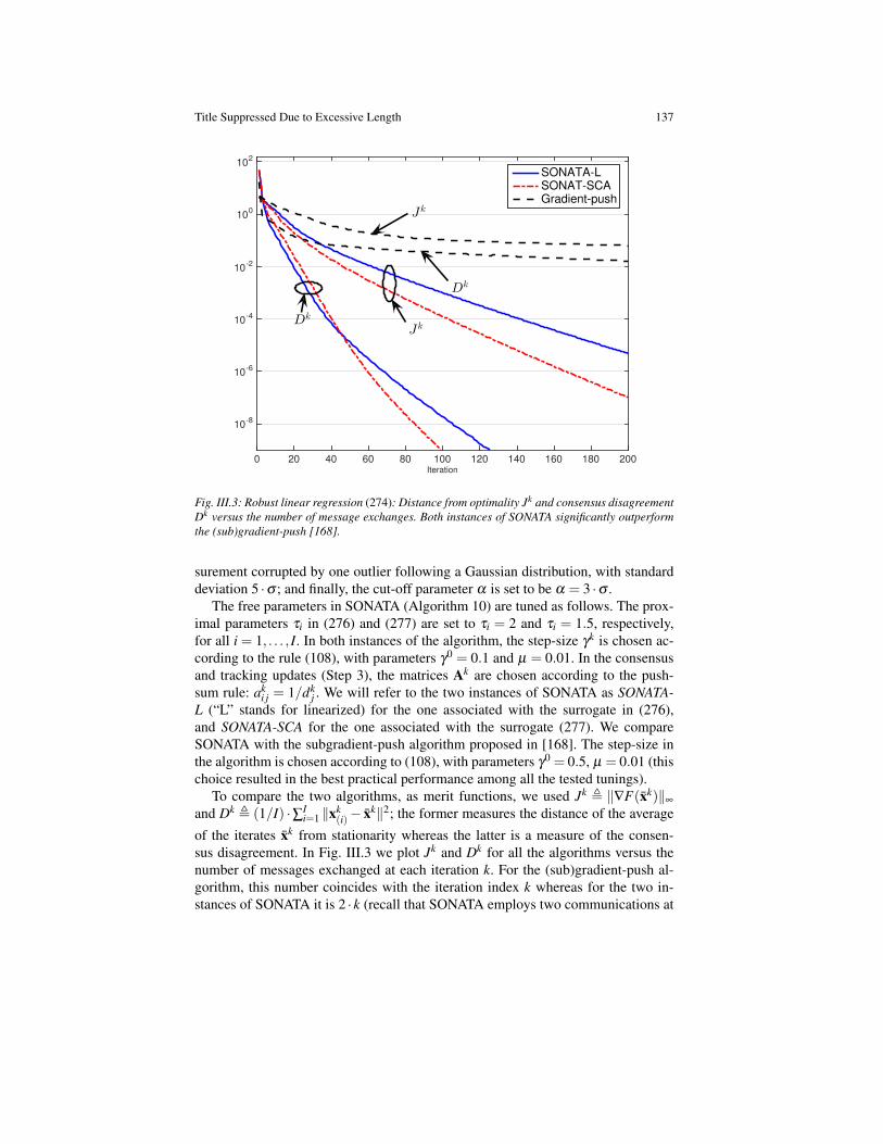
Title Suppressed Due to Excessive Length 137
Iteration
0 20 40 60 80 100 120 140 160 180 200
10-8
10-6
10-4
10-2
100
102
SONATA-LSONAT-SCAGradient-push
Jk
Dk
Dk
Jk
Fig. III.3: Robust linear regression (274): Distance from optimality Jk and consensus disagreementDk versus the number of message exchanges. Both instances of SONATA significantly outperformthe (sub)gradient-push [168].
surement corrupted by one outlier following a Gaussian distribution, with standarddeviation 5 ·σ ; and finally, the cut-off parameter α is set to be α = 3 ·σ .
The free parameters in SONATA (Algorithm 10) are tuned as follows. The prox-imal parameters τi in (276) and (277) are set to τi = 2 and τi = 1.5, respectively,for all i = 1, . . . , I. In both instances of the algorithm, the step-size γk is chosen ac-cording to the rule (108), with parameters γ0 = 0.1 and µ = 0.01. In the consensusand tracking updates (Step 3), the matrices Ak are chosen according to the push-sum rule: ak
i j = 1/dkj . We will refer to the two instances of SONATA as SONATA-
L (“L” stands for linearized) for the one associated with the surrogate in (276),and SONATA-SCA for the one associated with the surrogate (277). We compareSONATA with the subgradient-push algorithm proposed in [168]. The step-size inthe algorithm is chosen according to (108), with parameters γ0 = 0.5, µ = 0.01 (thischoice resulted in the best practical performance among all the tested tunings).
To compare the two algorithms, as merit functions, we used Jk , ‖∇F(xk)‖∞
and Dk , (1/I) ·∑Ii=1 ‖xk
(i)− xk‖2; the former measures the distance of the average
of the iterates xk from stationarity whereas the latter is a measure of the consen-sus disagreement. In Fig. III.3 we plot Jk and Dk for all the algorithms versus thenumber of messages exchanged at each iteration k. For the (sub)gradient-push al-gorithm, this number coincides with the iteration index k whereas for the two in-stances of SONATA it is 2 · k (recall that SONATA employs two communications at
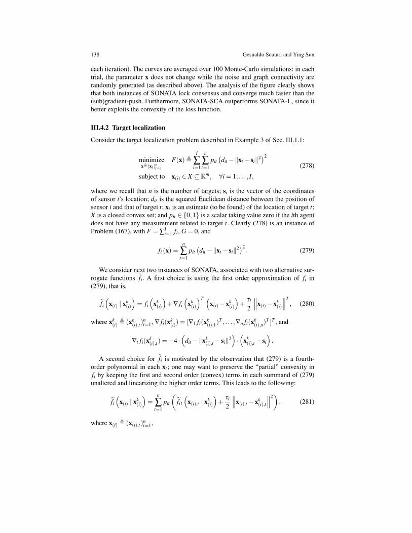
138 Gesualdo Scutari and Ying Sun
each iteration). The curves are averaged over 100 Monte-Carlo simulations: in eachtrial, the parameter x does not change while the noise and graph connectivity arerandomly generated (as described above). The analysis of the figure clearly showsthat both instances of SONATA lock consensus and converge much faster than the(sub)gradient-push. Furthermore, SONATA-SCA outperforms SONATA-L, since itbetter exploits the convexity of the loss function.
III.4.2 Target localization
Consider the target localization problem described in Example 3 of Sec. III.1.1:
minimizex,(xt )
nt=1
F(x),I
∑i=1
n
∑t=1
pit(dit −‖xt − si‖2)2
subject to x(i) ∈ X ⊆ Rm, ∀i = 1, . . . , I,
(278)
where we recall that n is the number of targets; si is the vector of the coordinatesof sensor i’s location; dit is the squared Euclidean distance between the position ofsensor i and that of target t; xt is an estimate (to be found) of the location of target t;X is a closed convex set; and pit ∈ 0,1 is a scalar taking value zero if the ith agentdoes not have any measurement related to target t. Clearly (278) is an instance ofProblem (167), with F = ∑
Ii=1 fi, G = 0, and
fi (x) =n
∑t=1
pit(dit −‖xt − si‖2)2
. (279)
We consider next two instances of SONATA, associated with two alternative sur-rogate functions fi. A first choice is using the first order approximation of fi in(279), that is,
fi
(x(i) | xk
(i)
)= fi
(xk(i)
)+∇ fi
(xk(i)
)T (x(i)−xk
(i)
)+
τi
2
∥∥∥x(i)−xk(i)
∥∥∥2, (280)
where xk(i) , (xk
(i),t)nt=1, ∇ fi(xk
(i)) = [∇1 fi(xk(i),1)
T , . . . ,∇n fi(xk(i),n)
T ]T , and
∇t fi(xk(i),t) =−4 ·
(dit −‖xk
(i),t − si‖2)·(
xk(i),t − si
).
A second choice for fi is motivated by the observation that (279) is a fourth-order polynomial in each xt ; one may want to preserve the “partial” convexity infi by keeping the first and second order (convex) terms in each summand of (279)unaltered and linearizing the higher order terms. This leads to the following:
fi
(x(i) | xk
(i)
)=
n
∑t=1
pit
(fi t
(x(i),t | xk
(i)
)+
τi
2
∥∥∥x(i),t −xk(i),t
∥∥∥2), (281)
where x(i) , (x(i),t)nt=1,
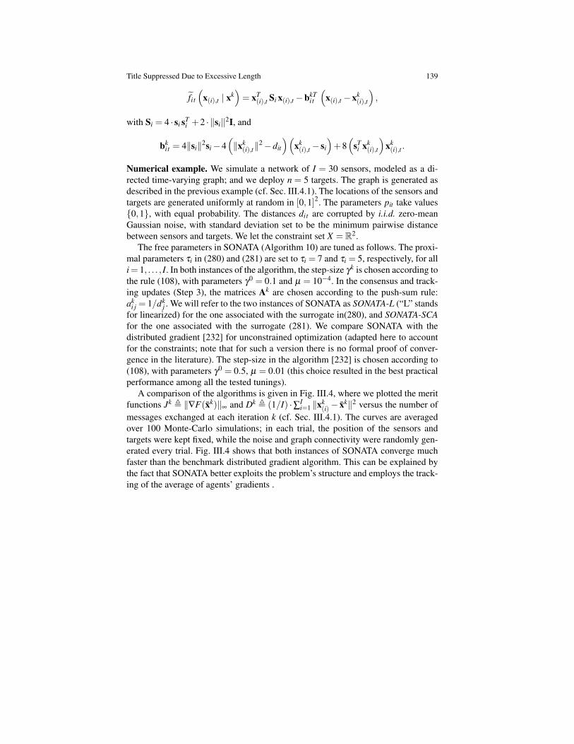
Title Suppressed Due to Excessive Length 139
fi t
(x(i),t | xk
)= xT
(i),t Si x(i),t −bkTit
(x(i),t −xk
(i),t
),
with Si = 4 · si sTi +2 · ‖si‖2I, and
bkit = 4‖si‖2si−4
(‖xk
(i),t‖2−dit
)(xk(i),t − si
)+8(
sTi xk
(i),t
)xk(i),t .
Numerical example. We simulate a network of I = 30 sensors, modeled as a di-rected time-varying graph; and we deploy n = 5 targets. The graph is generated asdescribed in the previous example (cf. Sec. III.4.1). The locations of the sensors andtargets are generated uniformly at random in [0,1]2. The parameters pit take values0,1, with equal probability. The distances di t are corrupted by i.i.d. zero-meanGaussian noise, with standard deviation set to be the minimum pairwise distancebetween sensors and targets. We let the constraint set X = R2.
The free parameters in SONATA (Algorithm 10) are tuned as follows. The proxi-mal parameters τi in (280) and (281) are set to τi = 7 and τi = 5, respectively, for alli= 1, . . . , I. In both instances of the algorithm, the step-size γk is chosen according tothe rule (108), with parameters γ0 = 0.1 and µ = 10−4. In the consensus and track-ing updates (Step 3), the matrices Ak are chosen according to the push-sum rule:ak
i j = 1/dkj . We will refer to the two instances of SONATA as SONATA-L (“L” stands
for linearized) for the one associated with the surrogate in(280), and SONATA-SCAfor the one associated with the surrogate (281). We compare SONATA with thedistributed gradient [232] for unconstrained optimization (adapted here to accountfor the constraints; note that for such a version there is no formal proof of conver-gence in the literature). The step-size in the algorithm [232] is chosen according to(108), with parameters γ0 = 0.5, µ = 0.01 (this choice resulted in the best practicalperformance among all the tested tunings).
A comparison of the algorithms is given in Fig. III.4, where we plotted the meritfunctions Jk , ‖∇F(xk)‖∞ and Dk , (1/I) ·∑I
i=1 ‖xk(i)− xk‖2 versus the number of
messages exchanged at each iteration k (cf. Sec. III.4.1). The curves are averagedover 100 Monte-Carlo simulations; in each trial, the position of the sensors andtargets were kept fixed, while the noise and graph connectivity were randomly gen-erated every trial. Fig. III.4 shows that both instances of SONATA converge muchfaster than the benchmark distributed gradient algorithm. This can be explained bythe fact that SONATA better exploits the problem’s structure and employs the track-ing of the average of agents’ gradients .
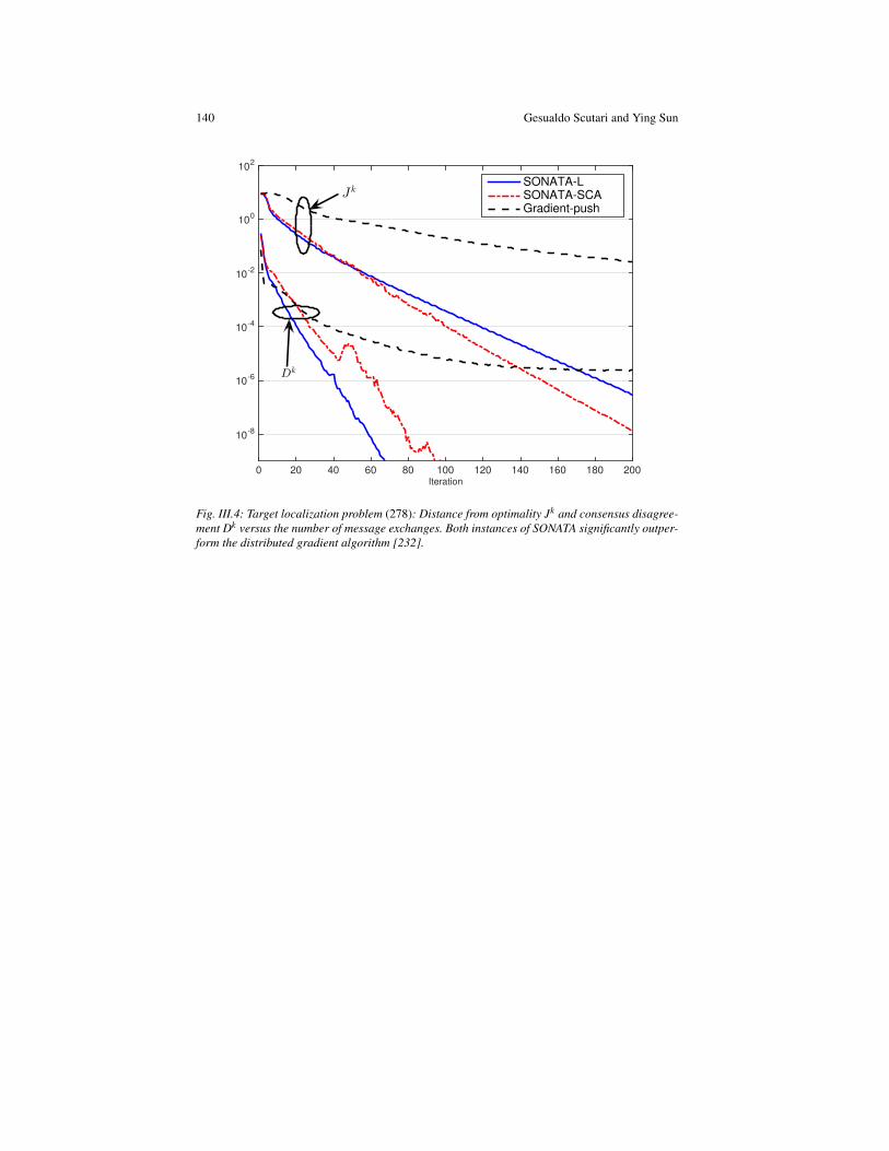
140 Gesualdo Scutari and Ying Sun
Iteration0 20 40 60 80 100 120 140 160 180 200
10-8
10-6
10-4
10-2
100
102
SONATA-LSONATA-SCAGradient-push
Jk
Dk
Fig. III.4: Target localization problem (278): Distance from optimality Jk and consensus disagree-ment Dk versus the number of message exchanges. Both instances of SONATA significantly outper-form the distributed gradient algorithm [232].

Title Suppressed Due to Excessive Length 141
III.5. Sources and NotesDistributed optimization has a rich literature, dating back to the 1980s [240]. Sincethen, due to the emergence of large-scale networks, advances in computing andstorage, data acquisition, and communications, the development of distributed algo-rithms for solving optimization problems over networks has received significant at-tention. Besides the distributed approaches we are going to summarize below, manyefforts have been made to solve optimization problems over networks with specifictopology, including multilayer HNets (e.g., master-slave architectures and shared-memory systems)–see Fig. III.1. However, all these schemes require some degreeof centralization to be implemented, due to the use of master nodes. Since the fo-cus of this lecture is on distributed algorithms implementable on general networkarchitectures, in the following we omit to discuss the literature on algorithms forHNets. Although the lecture considered mainly nonconvex optimization, we beginoverviewing the much abundant literature of distributed algorithms for convex prob-lems. In fact, some of the methods and tools introduced in this lecture for nonconvexproblems can be applied and are useful also for convex instances.
Distributed convex optimization
The literature on distributed solution methods for convex problems is vast and acomprehensive overview of current methods goes beyond the scope of this com-mentary. Here we briefly focus on the methods somehow related to the proposedSCA approach and distributed gradient tracking. Generally speaking, we roughlydivide the literature in two groups, namely: primal and dual methods.Primal methods. While substantially different, primal methods can be generi-cally abstracted as a combination of a local (sub)gradient step and a subsequentconsensus-like update (or multiple consensus updates); examples include [114,168,169,216,217]. Algorithms for adaptation and learning tasks based on in-network dif-fusion techniques were proposed in [39,46,201]. Schemes in [39,46,169,201,217]are applicable only to undirected graphs; [39, 169, 217] require the consensus ma-trices to be doubly-stochastic whereas [46, 201] use row-stochastic matrices but areapplicable only to strongly convex agents’ cost functions having a common min-imizer. When the graph is directed, doubly-stochastic weight matrices compliantto the graph may not exist; and, when they exist, their construction is computa-tionally prohibitive for networks with arbitrary topology [92]. Recently, some newalgorithms have been developed that do not require doubly-stochastic weights. Ex-amples, include [168], where the authors combined the sub-gradient algorithm [169]with the push-sum consensus protocol [121]; and [256,257]. However, the schemesin [169,256,257] considered only unconstrained optimization problems; in fact, upuntil the very recent works [211,230,231], it was not clear how to leverage push-sumprotocols to deal with constraints (e.g., to preserve the feasibility of the iterates).
In all the aforementioned algorithms but [211, 231], agents perform their localoptimization using only the gradient of their own function, while neglecting the restof the sum-cost function F [cf. (167)]. This makes the algorithms simple but usu-

142 Gesualdo Scutari and Ying Sun
ally slow: Even if the objective functions are differentiable and strongly convex,these methods still need to use a diminishing step-size to converge to a consensualsolution, and thus converge at a sub-linear rate. On the other hand, with a con-stant (sufficiently small) step-size, these distributed methods can be faster, but theyonly converge to a neighborhood of the solution set. This phenomenon creates anexactness-speed dilemma. In addition, convergence of these algorithms was provedonly under the assumption that the objective function has bounded (sub)gradient,which limits the range of applicability of these schemes.
A different class of distributed (primal) approaches that bypasses the above is-sues is the one based on the idea of gradient tracking: each agent updates its ownlocal variables along a surrogate direction that tracks the gradient average ∑i ∇ fi.This idea was proposed independently in [69, 70, 148] for the general class of con-strained nonsmooth nonconvex problems (167), and in [259] for the special caseof strongly convex, unconstrained, smooth, optimization. The works [211, 231] ex-tended the algorithms to (possibly) time-varying digraphs (still in the nonconvexsetting of [69, 70, 148]). A convergence rate analysis of the scheme [259] was laterdeveloped in [170,190], with [170] considering time-varying (directed) graphs. Thebenefit of these schemes is threefold: i) a constant step-size can be employed, insteadof a diminishing one; ii) the assumption that the gradient is bounded is no longerneeded; and iii) the convergence speed of the algorithms significantly improves–linear convergence was in fact proved in [170, 190] for unconstrained, smooth,strongly convex ∑i fi, and more recently in [229] for the more general class of con-strained, nonsmooth, problems (167) (with F strongly convex).
Finally, it is worth mentioning that a difference algorithmic structure was pro-posed in [216] to cancel the steady state error in the aforementioned plain decentral-ized gradient descent methods and converge to a consensual solution using a fixed(sufficiently small) step-size. Convergence at a sub-linear rate was proved when theobjective function is smooth and convex (and the problem unconstrained), and aQ-linear rate when the objective function is (smooth) strongly convex (still uncon-strained optimization).Dual-based methods: This class of algorithms is based on a different approach:slack variables are first introduced to decouple the sum-utility function while forc-ing consistency among these local copies by adding consensus equality constraints(matching the graph topology). Lagrangian dual variables are then introduced todeal with such coupling constraints. The resulting algorithms build on primal-dualupdates, aiming at converging to a saddle point of the (augmented) Lagrangian func-tion. Examples of such algorithms include ADMM-like methods [42,113,217,247]as well as inexact primal-dual instances wherein a first order [43] or second-order[163,164] approximation of the Lagrangian function is minimized at each iteration.All these algorithms can handle only static and undirected graphs. Dual methodscannot be trivially extended to time-varying graphs or digraphs, as it is not clearhow to enforce consensus via equality constraints over time-varying or directednetworks. Furthermore, all the above schemes but [42, 217] require the objectivefunction to be smooth and the optimization problem to be unconstrained.

Title Suppressed Due to Excessive Length 143
Proj-DGM[20]
NEXT[148]
Push-sumDGM[232]
Prox-PDA[106]
DeFW [245]SONATA [211]
(this chapter)
nonsmooth G+ X X
constraints X X X compact X
unbounded gradient X X
networktopology
:time-varying X X X
digraph restricted X X
step-size:constant X X
diminishing X X X X X X
complexity X X X X
Table III.3: Overview of current distributed methods for nonconvex optimization over networks.
III.5.1 Distributed nonconvex optimization
For the general nonconvex problem (167), results are scarse. We remark that theparallel algorithm described in Lecture II as well as those discussed in Sec. II.7are not applicable to the distributed setting (167): either they require the graph tobe complete (i.e., at each iteration, agents must be able to exchange informationwith all the others) or they assume full knowledge of F from the agents. Thereare only a few distributed algorithms designed for (167), including primal methods[20,148,232,245] and dual methods [106,275]. The key features of these algorithmsare summarized in Table III.3 and briefly discussed next.Primal methods: The distributed stochastic projection scheme [20] implementsrandom gossip between agents and uses diminishing step-size, and can handlesmooth objective functions over undirected static graphs. In [232], the authorsshowed that the distributed push-sum gradient algorithm with diminishing step-size,earlier proposed for convex objectives in [168], converges also when applied to non-convex smooth unconstrained problems. The first provably convergent distributedscheme for (167), with G 6= 0 and (convex) constraints X , over time-varying di-graphs is NEXT [69, 70, 148]. A special instance of NEXT, applied to smooth Vover undirected static graphs, was later proved in [245] to have sub-linear conver-gence rate. However, the consensus protocol employed in [148, 245] uses doubly-stochastic weight matrices, and thus is limited to special digraphs (or undirectedgraphs). Moreover, all the algorithms discussed above require that the (sub)gradientof V is bounded on X (or Rm).
This issue was resolved in SONATA (Algorithm 10, Sec. III.3), proposed in[211, 231], which combined a judiciously designed perturbed push-sum consensusscheme with SCA techniques. Based on a new line of analysis whereby optimiza-tion and consensus dynamics are jointly analyzed by introducing a novel Lyapunovfunction, SONATA was shown to converge sub-linearly to a stationary solution of(167), without requiring the (sub)gradient of V being bounded. SONATA is also thefirst provably convergent algorithm that i) can deal with constrained, nonsmooth,

144 Gesualdo Scutari and Ying Sun
(convex and nonconvex) problems in the form (167), and time-varying digraphs;and ii) employs either a constant or diminishing step-size.Dual-based methods: As their convex counterparts, dual-based schemes [106,275]cannot deal with time-varying or directed graphs. The algorithm proposed in [275] isan early attempt of distributed method for nonconvex problems. However, it calls forthe solution of nonconvex subproblems and converges to (stationary) solutions of anauxiliary problem, which are not necessarily stationary for the original problem. Theprox-PDA algorithm in [106], proposed for linearly constrained problems, can beapplied to Problem (167), but it is limited to the special classes where the functionsfi are smooth and X = Rm. The dual-based algorithms discussed above but [106]assume that the (sub)gradient of V is bounded.Practical implementation issues and open questions. The majority of the meth-ods discussed above assume an “ideal” distributed computing environment whereinall the communication links operate reliably and noise-free, and the agents commu-nicate and update their own variables in a synchronous fashion. There are howevermany practical issues that arise for these models, including difficulties associatedwith maintaining time-synchronization in face of computational and communica-tion delays, reaching deadlock situations requiring re-initializations of the updateprocess due to node/link failures.
Asynchronous methods based on randomization techniques were proposed in[18–20, 22, 110, 128, 140, 166, 174, 224, 247, 272]. These algorithms assume thatagents are activated (wakeup) randomly (with no coordination), run some lo-cal computation, and then wake up (some or all) their neighbors to pass themtheir most recent update. Both random (e.g., based on gossip consensus schemes)[18–20, 110, 140, 166, 224, 247, 272] and deterministic (e.g., based on the push-sumprotocol) activations [22, 128, 174] of the neighbors were proposed. While asyn-chronous in the activation of the agents performing the update, these schemes stillimpose a coordination among the agents, cannot tolerate (arbitrary) delays in thecommunications (packet losses are considered in [22, 128, 272]) or optimization(out-of-sync information), and require the agents to stay all the time in listeningmode. A first attempt to deal with this issue was proposed in [255]: a dual-basedscheme is employed wherein agents are randomly activated, and update their localcopies using possibly outdated information. The probabilistic model for asynchronyrequires that the random variables triggering the activation of the agents and thedelay vector used by the agent to performs its update are independent. While thisgreatly simplifies the convergence analysis, it makes the model not realistic–seeSec. II.7 in Lec. II for a discussion on this issue. Furthermore, [255] is applicableonly to convex instances of (167), and over fixed undirected graphs. At the time ofthis writing, designing distributed fully asynchronous algorithms for the nonconvexproblem (167)–in the sense that i) agents update their own variables with no coordi-nation; and ii) can handle arbitrary (deterministic or random) delay profiles–remainsan open problem. A first attempt towards this direction can be found in [234].
Despite of asynchrony, another question of practical interest is how to designand implement distributed algorithms under low communication requirements, andwhat trade-offs are involved in such designs/implementations. For instance, in some
Title Suppressed Due to Excessive Length 145
sensor networks, broadcast communications can be too expensive in terms of con-sumed power. Also, communications are subject to rate constraints (systems arebandwidth limited). Furthermore, in the emerging distributed big-data applications,optimization problems are huge-scale: computing at each iteration the gradient withrespect to all the optimization variables, communicating at each iteration, and send-ing to the neighbors the entire set of variables would incur in an unaffordable com-putational cost and communication overhead or is just infeasible. Some initial in-vestigations along this lines were presented in the literature, following alternative,scattered, paths. For instance, in [175, 176], a distributed algorithm for convex andnonconvex instances of (167) was proposed, aiming at reducing both communica-tion and computation costs by optimizing and transmitting at each iteration onlya subset of the entire optimization variables. While asymptotic convergence of themethod was proved, the tradeoff between communication and computation has notbeen studied yet. Some insight on the impact of multiple communications steps(without optimizing) or multiple optimization steps (without communicating) canbe found in [13,239]. Finally, some works proposed distributed methods for convexoptimization problems implementing quantized communications. Of course, muchmore research needs to be done on these important topics.

146 Gesualdo Scutari and Ying Sun
References
1. 3GPP TR 36.814.2. M. Ahn, J.-S. Pang, and J. Xin. Difference-of-convex learning: Directional stationarity, op-
timality, and sparsity. SIAM Journal on Optimization, 27(3):1637–1665, 2017.3. M. Allain, J. Idier, and Y. Goussard. On global and local convergence of half-quadratic
algorithms. IEEE Transactions on Image Processing, 15(5):1130–1142, 2006.4. F. Bach, R. Jenatton, J. Mairal, and G. Obozinski. Optimization with sparsity-inducing penal-
ties. Foundations and Trends R© in Machine Learning, 4(1):1–106, 2012.5. G. M. Baudet. Asynchronous iterative methods for multiprocessors. Journal of the ACM
(JACM), 25(2):226–244, 1978.6. E. Bauer, D. Koller, and Y. Singer. Update rules for parameter estimation in bayesian net-
works. In Proceedings of the Thirteenth Conference on Uncertainty in Artificial Intelligence,pages 3–13, 1997.
7. A. Beck and M. Teboulle. A fast iterative shrinkage-thresholding algorithm for linear inverseproblems. SIAM Journal on Imaging Sciences, 2(1):183–202, 2009.
8. A. Beck and M. Teboulle. Gradient-based algorithms with applications to signal recoveryproblems. In Convex Optimization in Signal Processing and Communications, chapter 2.Cambridge University Press, Cambridge, UK, 2010.
9. A. Beck, M. Teboulle, and Z. Chikishev. Iterative minimization schemes for solving thesingle source localization problem. SIAM Journal on Optimization, 19(3):1397–1416, 2008.
10. M. P. Becker, I. Yang, and K. Lange. EM algorithms without missing data. StatisticalMethods in Medical Research, 6(1):38–54, 1997.
11. F. Bénézit, V. Blondel, P. Thiran, J. Tsitsiklis, and M. Vetterli. Weighted gossip: Distributedaveraging using non-doubly stochastic matrices. In Proceedings of the 2010 IEEE interna-tional symposium on Information theory proceedings (ISIT), pages 1753–1757, 2010.
12. K. Benidis, Y. Sun, P. Babu, and D. P. Palomar. Orthogonal sparse PCA and covariance esti-mation via procrustes reformulation. IEEE Transactions on Signal Processing, 64(23):6211–6226, 2016.
13. A. S. Berahas, R. Bollapragada, N. S. Keskar, and E. Wei. Balancing communication andcomputation in distributed optimization. arXiv preprint, arXiv:1709.02999, 2017.
14. D. P. Bertsekas. Nonlinear Programming. Athena Scientific, 1995.15. D. P. Bertsekas and P. Tseng. Partial proximal minimization algorithms for convex ppro-
gramming. SIAM Journal on Optimization, 4(3):551–572, 1994.16. D. P. Bertsekas and J. N. Tsitsiklis. Parallel and Distributed Computation: Numerical Meth-
ods. Athena Scientific Press, 2nd edition, 1989.17. D. P. Bertsekas and J. N. Tsitsiklis. Gradient convergence in gradient methods with errors.
SIAM Journal on Optimization, 10(3):627–642, 2000.18. P. Bianchi, G. Fort, and W. Hachem. Performance of a distributed stochastic approximation
algorithm. IEEE Transactions on Information Theory, 59(11):7405–7418, 2013.19. P. Bianchi, W. Hachem, and F. Iutzeler. A coordinate descent primal-dual algorithm and
application to distributed asynchronous optimization. IEEE Transactions on Automatic Con-trol, 61(10):2947–2957, 2016.
20. P. Bianchi and J. Jakubowicz. Convergence of a multi-agent projected stochastic gradient al-gorithm for non-convex optimization. IEEE Transactions on Automatic Control, 58(2):391–405, 2013.
21. T. Blumensath, M. Yaghoobi, and M. E. Davies. Iterative hard thresholding and l0 regularisa-tion. In Proceedings of the IEEE International Conference on Acoustics, Speech and SignalProcessing (ICASSP 2007), volume 3, pages 877–880, 2007.
22. N. Bof, R. Carli, G. Notarstefano, L. Schenato, and D. Varagnolo. Newton-Raphson consen-sus under asynchronous and lossy communications for peer-to-peer networks. arXiv preprint,arXiv:1707.09178, 2017.
23. D. Böhning. Multinomial logistic regression algorithm. Annals of the Institute of StatisticalMathematics, 44(1):197–200, 1992.

Title Suppressed Due to Excessive Length 147
24. J. M. Borwein and A. S. Lewis. Convex Analysis and Nonlinear Optimization: Theory andExamples. CMS Books in Mathematics, Springer, 2000.
25. L. Bottou, F. E. Curtis, and J. Nocedal. Optimization methods for large-scale machine learn-ing. arXiv preprint, arXiv:1606.04838, 2016.
26. C. Bouman and K. Sauer. Fast numerical methods for emission and transmission tomo-graphic reconstruction. In Proceedings of Conference on Information Sciences and Systems,pages 611–616, 1993.
27. R. A. Boyles. On the convergence of the EM algorithm. Journal of the Royal StatisticalSociety. Series B (Methodological), pages 47–50, 1983.
28. Joseph K Bradley, Aapo Kyrola, Danny Bickson, and Carlos Guestrin. Parallel coordinatedescent for l1-regularized loss minimization. In Proceedings of the 28th International Con-ference on Machine Learning (ICML 2011), pages 321–328, 2011.
29. P. S. Bradley and O. L. Mangasarian. Feature selection via concave minimization and sup-port vector machines. In Proceedings of the Fifteenth International Conference on MachineLearning (ICML 98’), volume 98, pages 82–90, 1998.
30. P. Bühlmann and S. van De Geer. Statistics for high-dimensional data: methods, theory andapplications. Springer-Verlag Berlin Heidelberg, 2011.
31. R. H. Byrd, J. Nocedal, and F. Oztoprak. An inexact successive quadratic approxima-tion method for l-1 regularized optimization. Mathematical Programming, 157(2):375–396,2016.
32. E. J. Candés, X. Li, Y. Ma, and J. Wright. Robust principal component analysis? Journal ofthe ACM (JACM), 58(3):11, 2011.
33. E. J. Candés and T. Tao. Decoding by linear programming. IEEE Transactions on Informa-tion Theory, 51(12):4203–4215, 2005.
34. E. J. Candés and T. Tao. Near-optimal signal recovery from random projections: Universalencoding strategies? IEEE Transactions on Information Theory, 52(12):5406–5425, 2006.
35. E. J. Candés and M. B. Wakin. An introduction to compressive sampling. IEEE SignalProcessing Magazine, 25(2):21–30, 2008.
36. E. J. Candés, M. B. Wakin, and S. P. Boyd. Enhancing sparsity by reweighted `1 minimiza-tion. Journal of Fourier Analysis and Applications, 14(5-6):877–905, 2008.
37. L. Cannelli, F. Facchinei, V. Kungurtsev, and G. Scutari. Asynchronous parallel algo-rithms for nonconvex big-data optimization: Model and convergence. arXiv preprint,arXiv:1607.04818, 2016.
38. L. Cannelli, F. Facchinei, V. Kungurtsev, and G. Scutari. Asynchronous parallel algo-rithms for nonconvex big-data optimization Part II: Complexity and numerical results. arXivpreprint, arXiv:1701.04900, 2017.
39. F. S. Cattivelli and A. H. Sayed. Diffusion LMS strategies for distributed estimation. IEEETransactions on Signal Processing, 58(3):1035–1048, 2010.
40. A. Chambolle. An algorithm for total variation minimization and applications. Journal ofMathematical Imaging and Vision, 20(1–2):89–97, Jan. 2004.
41. V. Chandrasekaran, S. Sanghavi, P. A. Parrilo, and A. S. Willsky. Rank-sparsity incoherencefor matrix decomposition. SIAM Journal on Optimization, 21(2):572–596, 2011.
42. T.-H. Chang. A proximal dual consensus ADMM method for multi-agent constrained opti-mization. IEEE Transactions on Signal Processing, 64(14):3719–3734, 2014.
43. T.-H. Chang, M. Hong, and X. Wang. Multi-agent distributed optimization via inexact con-sensus ADMM. IEEE Transactions on Signal Processing, 63(2):482–497, 2015.
44. T. Charalambous, M. G. Rabbat, M. Johansson, and C. N. Hadjicostis. Distributed finite-time computation of digraph parameters: Left-eigenvector, out-degree and spectrum. IEEETransactions on Control of Network Systems, 3(2):137–148, 2016.
45. D. Chazan and W. Miranker. Chaotic relaxation. Linear Algebra and its Applications,2(2):199–222, 1969.
46. J. Chen and A. H. Sayed. Diffusion adaptation strategies for distributed optimization andlearning over networks. IEEE Transactions on Signal Processing, 60(8):4289–4305, 2012.
148 Gesualdo Scutari and Ying Sun
47. E. Chouzenoux, J. Idier, and S. Moussaoui. A majorize-minimize strategy for subspace opti-mization applied to image restoration. IEEE Transactions on Image Processing, 20(6):1517–1528, 2011.
48. E. Chouzenoux, S. Moussaoui, and J. Idier. Majorize-minimize linesearch for inversionmethods involving barrier function optimization. Inverse Problems, 28(6):065011, 2012.
49. E. Chouzenoux and J.-C. Pesquet. Convergence rate analysis of the majorize-minimize sub-space algorithm. IEEE Signal Processing Letters, 23(9):1284–1288, 2016.
50. E. Chouzenoux, J.-C. Pesquet, and A. Repetti. Variable metric forward-backward algorithmfor minimizing the sum of a differentiable function and a convex function. Journal of Opti-mization Theory and Applications, 162(1):107–132, 2014.
51. G. Cohen. Optimization by decomposition and coordination: A unified approach. IEEETransactions on Automatic Control, 23(2):222–232, 1978.
52. G. Cohen. Auxiliary problem principle and decomposition of optimization problems. Journalof Optimization Theory and Applications, 32(3):277–305, 1980.
53. P. L. Combettes and J.-C. Pesquet. Proximal splitting methods in signal processing. In Fixed-point Algorithms for Inverse Problems in Science and Engineering, pages 185–212. Springer,2011.
54. J. A. Costa, N. Patwari, and A. O. Hero III. Distributed weighted-multidimensional scalingfor node localization in sensor networks. ACM Transactions on Sensor Networks (TOSN),2(1):39–64, 2006.
55. A. Daneshmand. Numerical Comparison of Hybrid Random/Deterministic Parallel Algo-rithms for nonconvex big data Optimization. Technical report, Dept. of Elect. Eng., SUNYBuffalo, August 2014.
56. A. Daneshmand, F. Facchinei, V. Kungurtsev, and G. Scutari. Hybrid random/deterministicparallel algorithms for convex and nonconvex big data optimization. IEEE Transactions onSignal Processing, 63(15):3914–3929, 2015.
57. J. M. Danskin. The theory of max-min, with applications. SIAM Journal on Applied Mathe-matics, 14(4):641–664, 1966.
58. M. E. Daube-Witherspoon and G. Muehllehner. An iterative image space reconstructionalgorthm suitable for volume ECT. IEEE Transactions on Medical Imaging, 5(2):61–66,1986.
59. I. Daubechies, M. Defrise, and C. De Mol. An iterative thresholding algorithm for linearinverse problems with a sparsity constraint. Communications on Pure and Applied Mathe-matics, 57(11):1413–1457, 2004.
60. D. Davis. The asynchronous PALM algorithm for nonsmooth nonconvex problems. arXivpreprint, arXiv:1604.00526, 2016.
61. D. Davis, B. Edmunds, and M. Udell. The sound of APALM clapping: Faster nonsmoothnonconvex optimization with stochastic asynchronous PALM. In Advances in Neural Infor-mation Processing Systems 29 (NIPS 2016), pages 226–234. Curran Associates, Inc., 2016.
62. J. de Leeuw. Applications of convex analysis to multidimensional scaling. In Recent Devel-opments in Statistics, 1977.
63. J. de Leeuw. Convergence of the majorization method for multidimensional scaling. Journalof Classification, 5(2):163–180, 1988.
64. J. de Leeuw. Block-relaxation algorithms in statistics. In Information Systems and DataAnalysis, pages 308–324. Springer, 1994.
65. J. de Leeuw and W. J. Heiser. Convergence of correction matrix algorithms for multidimen-sional scaling. Geometric Representations of Relational Data, pages 735–752, 1977.
66. A. P. Dempster, N. M. Laird, and D. B. Rubin. Maximum likelihood from incomplete datavia the EM algorithm. Journal of the Royal Statistical Society. Series B (methodological),pages 1–38, 1977.
67. W. Deng, M.-J. Lai, Z. Peng, and W. Yin. Parallel multi-block ADMM with o(1/k) conver-gence. Journal of Scientific Computing, 71(2):712–736, 2017.
68. I. S. Dhillon, P. K. Ravikumar, and A. Tewari. Nearest neighbor based greedy coordinatedescent. In Advances in Neural Information Processing Systems 24 (NIPS 2011), pages2160–2168. Curran Associates, Inc., 2011.

Title Suppressed Due to Excessive Length 149
69. P. Di Lorenzo and G. Scutari. Distributed nonconvex optimization over networks. In Pro-ceedings of the IEEE 6th International Workshop on Computational Advances in Multi-Sensor Adaptive Processing (CAMSAP 2015), 2015.
70. P. Di Lorenzo and G. Scutari. Distributed nonconvex optimization over time-varying net-works. In Proceedings of the IEEE International Conference on Acoustics, Speech, andSignal Processing (ICASSP 2016), 2016.
71. S. Doclo, S. Gannot, M. Moonen, and A. Spriet. Acoustic beamforming for hearing aidapplications. Handbook on array processing and sensor networks, pages 269–302, 2010.
72. S. Doclo, M. Moonen, T. V. den Bogaert, and J. Wouters. Reduced-bandwidth and distributedMWF-based noise reduction algorithms for binaural hearing aids. IEEE Transactions onAudio, Speech, and Language Processing, 17(1):38–51, 2009.
73. P. B. Eggermont. Multiplicative iterative algorithms for convex programming. Linear Alge-bra and its Applications, 130:25–42, 1990.
74. H. A. Eiselt and V. Marianov. Pioneering developments in location analysis. In Foundationsof Location Analysis, International Series in Operations Research & Management Science,chapter 11, pages 3–22. Springer, 2011.
75. M. Elad and M. Aharon. Image denoising via sparse and redundant representations overlearned dictionaries. IEEE Transactions on Image processing, 15(12):3736–3745, 2006.
76. F. Facchinei, V. Kungurtsev, L. Lampariello, and G. Scutari. Ghost penalties in nonconvexconstrained optimization: Diminishing stepsizes and iteration complexity. arXiv preprint,arXiv:1709.03384, 2017.
77. F. Facchinei, L. Lampariello, and G. Scutari. Feasible methods for nonconvex nonsmoothproblems with applications in green communications. Mathematical Programming, 164(1-2):55–90, 2017.
78. F. Facchinei and J.-S. Pang. Finite-Dimensional Variational Inequalities and Complemen-tarity Problem. Springer-Verlag, New York, 2003.
79. F. Facchinei, G. Scutari, and S. Sagratella. Parallel selective algorithms for nonconvex bigdata optimization. IEEE Transactions on Signal Processing, 63(7):1874–1889, 2015.
80. J. Fan and R. Li. Variable selection via nonconcave penalized likelihood and its oracleproperties. Journal of the American statistical Association, 96(456):1348–1360, 2001.
81. J. A. Fessler and A. O. Hero III. Space-alternating generalized expectation-maximizationalgorithm. IEEE Transactions on Signal Processing, 42(10):2664–2677, 1994.
82. J. A. Fessler and A. O. Hero III. Penalized maximum-likelihood image reconstruction us-ing space-alternating generalized em algorithms. IEEE Transactions on Image Processing,4(10):1417–1429, 1995.
83. C. Févotte. Majorization-minimization algorithm for smooth Itakura-Saito nonnegative ma-trix factorization. In Proceedings of the IEEE International Conference on Acoustics, Speechand Signal Processing (ICASSP 2011), pages 1980–1983, 2011.
84. C. Févotte and J. Idier. Algorithms for nonnegative matrix factorization with the β -divergence. Neural Computation, 23(9):2421–2456, 2011.
85. M. A. T. Figueiredo, J. M. Bioucas-Dias, and R. D. Nowak. Majorization-minimizationalgorithms for wavelet-based image restoration. IEEE Transactions on Image processing,16(12):2980–2991, 2007.
86. M. A. T. Figueiredo and R. D. Nowak. A bound optimization approach to wavelet-basedimage deconvolution. In Proceedings of the IEEE International Conference on Image Pro-cessing (ICIP 2005), volume 2, 2005.
87. A. Frommer and D. B. Szyld. On asynchronous iterations. Journal of Computational andApplied Mathematics, 123(1-2):201–216, 2000.
88. W. J. Fu. Penalized regressions: the bridge versus the lasso. Journal of Computational andGraphical Statistics, 7(3):397–416, 1998.
89. M. Fukushima and H. Mine. A generalized proximal point algorithm for certain non-convexminimization problems. International Journal of Systems Science, 12(8):989–1000, 1981.
90. D. Geman and G. Reynolds. Constrained restoration and the recovery of discontinuities.IEEE Transactions on pattern analysis and machine intelligence, 14(3):367–383, 1992.
150 Gesualdo Scutari and Ying Sun
91. D. Geman and C. Yang. Nonlinear image recovery with half-quadratic regularization. IEEETransactions on Image Processing, 4(7):932–946, 1995.
92. B. Gharesifard and J. Cortés. When does a digraph admit a doubly stochastic adjacencymatrix? In Proceedings of the 2010 American Control Conference, pages 2440–2445, 2010.
93. G. B. Giannakis, V. Kekatos, N. Gatsis, S.-J. Kim, H. Zhu, and B. F. Wollenberg. Monitoringand optimization for power grids: A signal processing perspective. IEEE Signal ProcessingMagazine, 30(5):107–128, 2013.
94. I. F. Gorodnitsky and B. D. Rao. Sparse signal reconstruction from limited data using FO-CUSS: A re-weighted minimum norm algorithm. IEEE Transactions on Signal Processing,45(3):600–616, 1997.
95. J.-M. Gracia. Directional derivatives of the singular values of matrices depending on severalreal parameters. arXiv preprint, arXiv:1504.01679, 2015.
96. T. Hastie, R. Tibshirani, and J. Friedman. The elements of statistical learning. SpringerSeries in Statistics. Springer, New York, 2009.
97. T. Hastie, R. Tibshirani, and M. Wainwright. Statistical learning with sparsity: the lasso andgeneralizations. CRC Press, Taylor & Francis Group, 2015.
98. Z. He, S. Xie, R. Zdunek, G. Zhou, and A. Cichocki. Symmetric nonnegative matrix fac-torization: Algorithms and applications to probabilistic clustering. IEEE Transactions onNeural Networks, 22(12):2117–2131, 2011.
99. W. J. Heiser. Convergent computation by iterative majorization: theory and applications inmultidimensional data analysis. Recent Advances in Descriptive Multivariate Analysis, pages157–189, 1995.
100. D. P. Helmbold, R. E. Schapire, Y. Singer, and M. K. Warmuth. A comparison of new andold algorithms for a mixture estimation problem. Machine Learning, 27(1):97–119, 1997.
101. J. M. Hendrickx and J. N. Tsitsiklis. Fundamental limitations for anonymous distributedsystems with broadcast communications. In Proceedings of the 2015 53rd Annual AllertonConference on Communication, Control, and Computing (Allerton), pages 9–16, 2015.
102. J.-B. Hiriart-Urruty and C. Lemaréchal. Convex analysis and minimization algorithms I:Fundamentals, volume 305. Springer-Verlag Berlin Heidelberg, 1993.
103. A. Hjorungnes. Complex-Valued Matrix Derivatives With Applications in Signal Processingand Communications. Cambridge University Press, London, May 2011.
104. W. Hogan. Point-to-set maps in mathematical programming. SIAM Review, 15(3):591–603,1973.
105. M. Hong. A distributed, asynchronous and incremental algorithm for nonconvex optimiza-tion: An ADMM approach. IEEE Transactions on Control of Network Systems, 2017.
106. M. Hong, D. Hajinezhad, and M.-M. Zhao. Prox-PDA: The proximal primal-dual algorithmfor fast distributed nonconvex optimization and learning over networks. In Proceedings ofthe 34th International Conference on Machine Learning (ICML 2017), volume 70, pages1529–1538, 2017.
107. P. O. Hoyer. Non-negative matrix factorization with sparseness constraints. Journal of Ma-chine Learning Research, 5:1457–1469, Nov. 2004.
108. D. R. Hunter and K. Lange. A tutorial on MM algorithms. The American Statistician,58(1):30–37, 2004.
109. Z. Huo and H. Huang. Asynchronous stochastic gradient descent with variance reduction fornon-convex optimization. arXiv preprint, arXiv:1604.03584, 2016.
110. F. Iutzeler, P. Bianchi, P. Ciblat, and W. Hachem. Asynchronous distributed optimizationusing a randomized alternating direction method of multipliers. In Proceedings of the 2013IEEE 52nd Annual Conference on Decision and Control (CDC 2013), pages 3671–3676,2013.
111. M. W. Jacobson and J. A. Fessler. An expanded theoretical treatment of iteration-dependentmajorize-minimize algorithms. IEEE Transactions on Image Processing, 16(10):2411–2422,2007.
112. P. Jain, P. Netrapalli, and S. Sanghavi. Low-rank matrix completion using alternating mini-mization. In Proceedings of the Forty-Fifth Annual ACM Symposium on Theory of Comput-ing, pages 665–674, 2013.

Title Suppressed Due to Excessive Length 151
113. D. Jakovetic, J. Xavier, and J. M. F. Moura. Cooperative convex optimization in networkedsystems: Augmented Lagrangian algorithms with directed gossip communication. IEEETransactions on Signal Processing, 59(8):3889–3902, 2011.
114. D. Jakovetic, J. Xavier, and J. M. F. Moura. Fast distributed gradient methods. IEEE Trans-actions on Automatic Control, 59(5):1131–1146, 2014.
115. M. Jamshidian and R. I. Jennrich. Conjugate gradient acceleration of the EM algorithm.Journal of the American Statistical Association, 88(421):221–228, 1993.
116. M. Jamshidian and R. I. Jennrich. Acceleration of the EM algorithm by using quasi-Newton methods. Journal of the Royal Statistical Society: Series B (Statistical Methodology),59(3):569–587, 1997.
117. R. Jenatton, G. Obozinski, and F. Bach. Structured sparse principal component analysis. InProceedings of the Thirteenth International Conference on Artificial Intelligence and Statis-tics (AISTATS 2010), pages 366–373, 2010.
118. M. Journée, Y. Nesterov, P. Richtárik, and R. Sepulchre. Generalized power method forsparse principal component analysis. Journal of Machine Learning Research, 11(Feb):517–553, 2010.
119. N. Karowski, A. C. Viana, and A. Wolisz. Optimized asynchronous multi-channel neighbordiscovery. In Proceedings of the IEEE International Conference on Computer Communica-tions (INFOCOM 2011), pages 536–540, 2011.
120. V. Kekatos and G. B. Giannakis. Distributed robust power system state estimation. IEEETransactions on Power Systems, 28(2):1617–1626, 2013.
121. D. Kempe, A. Dobra, and J. Gehrke. Gossip-based computation of aggregate information.In Proceedings of the 44th Annual IEEE Symposium on Foundations of Computer Science,pages 482–491, 2003.
122. H. Kim and H. Park. Nonnegative matrix factorization based on alternating nonnegativityconstrained least squares and active set method. SIAM Journal on Matrix Analysis and Ap-plications, 30(2):713–730, 2008.
123. S.-J. Kim and G. B. Giannakis. Optimal resource allocation for MIMO ad hoc cognitiveradio networks. IEEE Transactions on Information Theory, 57(5):3117–3131, 2011.
124. K. Kreutz-Delgado. The complex gradient operator and the CR-calculus. Technical report,Electrical and Computer Engineering, Jacobs School of Engineering, University of Califor-nia, San Diego, July 2009.
125. B. Krishnapuram, L. Carin, M. A. T. Figueiredo, and A. J. Hartemink. Sparse multinomiallogistic regression: Fast algorithms and generalization bounds. IEEE Transactions on PatternAnalysis and Machine Intelligence, 27(6):957–968, 2005.
126. D. Kuang, C. Ding, and H. Park. Symmetric nonnegative matrix factorization for graphclustering. In Proceedings of the 2012 SIAM International Conference on Data Mining,pages 106–117, 2012.
127. D. Kuang, S. Yun, and H. Park. SymNMF: nonnegative low-rank approximation of a simi-larity matrix for graph clustering. Journal of Global Optimization, 62(3):545–574, 2015.
128. S. Kumar, R. Jain, and K. Rajawat. Asynchronous optimization over heterogeneous networksvia consensus ADMM. IEEE Transactions on Signal and Information Processing over Net-works, 3(1):114–129, 2017.
129. C. Labat and J. Idier. Convergence of conjugate gradient methods with a closed-form stepsizeformula. Journal of Optimization Theory and Applications, 136(1):43–60, 2008.
130. A. Lakhina, K. Papagiannaki, M. Crovella, C. Diot, E. D. Kolaczyk, and N. Taft. Structuralanalysis of network traffic flows. In ACM SIGMETRICS Performance evaluation review,volume 32, pages 61–72, 2004.
131. K. Lange. A gradient algorithm locally equivalent to the EM algorithm. Journal of the RoyalStatistical Society. Series B (Methodological), pages 425–437, 1995.
132. K. Lange. A quasi-Newton acceleration of the EM algorithm. Statistica Sinica, pages 1–18,1995.
133. K. Lange, E. C. Chi, and H. Zhou. A brief survey of modern optimization for statisticians.International Statistical Review, 82(1):46–70, 2014.
152 Gesualdo Scutari and Ying Sun
134. K. Lange and J. A. Fessler. Globally convergent algorithms for maximum a posteriori trans-mission tomography. IEEE Transactions on Image Processing, 4(10):1430–1438, 1995.
135. K. Lange, D. R. Hunter, and I. Yang. Optimization transfer using surrogate objective func-tions. Journal of Computational and Graphical Statistics, 9(1):1–20, 2000.
136. K. Lange and H. Zhou. MM algorithms for geometric and signomial programming. Mathe-matical Programming, 143(1-2):339–356, 2014.
137. R. Leblond, F. Pedregosa, and S. Lacoste-Julien. ASAGA: Asynchronous parallel SAGA.Proceedings of the 20th International Conference on Artificial Intelligence and Statistics(AISTATS), pages 46–54, 2017.
138. D. D. Lee and H. S. Seung. Learning the parts of objects by non-negative matrix factorization.Nature, 401(6755):788, 1999.
139. D. D. Lee and H. S. Seung. Algorithms for non-negative matrix factorization. In T. K. Leen,T. G. Dietterich, and V. Tresp, editors, Advances in Neural Information Processing Systems13 (NIPS 2000), pages 556–562. MIT Press, 2001.
140. S. Lee and A. Nedic. Asynchronous gossip-based random projection algorithms over net-works. IEEE Transactions on Automatic Control, 61(4):953–968, 2016.
141. R. M. Lewitt and G. Muehllehner. Accelerated iterative reconstruction for positron emissiontomography based on the EM algorithm for maximum likelihood estimation. IEEE Transac-tions on Medical Imaging, 5(1):16–22, 1986.
142. M. Li, L. Zhou, Z. Yang, A. Li, F. Xia, D. G. Andersen, and A. Smola. Parameter server fordistributed machine learning. In Big Learning NIPS Workshop, volume 6, page 2, 2013.
143. Y. Li and S. Osher. Coordinate descent optimization for `1 minimization with applicationto compressed sensing; a greedy algorithm. Inverse Problems and Imaging, 3(3):487–503,2009.
144. X. Lian, Y. Huang, Y. Li, and J. Liu. Asynchronous parallel stochastic gradient for nonconvexoptimization. In Advances in Neural Information Processing Systems 28 (NIPS 2015), pages2737–2745. Curran Associates, Inc., 2015.
145. T. Lipp and S. Boyd. Variations and extension of the convex-concave procedure. Optimiza-tion and Engineering, 17(2):263–287, 2016.
146. J. Liu and S. J. Wright. Asynchronous stochastic coordinate descent: Parallelism and con-vergence properties. SIAM Journal on Optimization, 25(1):351–376, 2015.
147. J. Liu, S. J. Wright, C. Ré, V. Bittorf, and S. Sridhar. An asynchronous parallel stochasticcoordinate descent algorithm. The Journal of Machine Learning Research, 16(1):285–322,2015.
148. P. Di Lorenzo and G. Scutari. NEXT: In-network nonconvex optimization. IEEE Transac-tions on Signal and Information Processing over Networks, 2(2):120–136, 2016.
149. Y. Lou, P. Yin, and J. Xin. Point source super-resolution via non-convex l1 based methods.Journal of Scientific Computing, 68(3):1082–1100, 2016.
150. T. A. Louis. Finding the observed information matrix when using the EM algorithm. Journalof the Royal Statistical Society. Series B (Methodological), pages 226–233, 1982.
151. J. Mairal. Incremental majorization-minimization optimization with application to large-scale machine learning. SIAM Journal on Optimization, 25(2):829–855, 2015.
152. O. L. Mangasarian. Machine Learning via Polyhedral Concave Minimization, pages 175–188. Physica-Verlag HD, Heidelberg, 1996.
153. H. Mania, X. Pan, D. Papailiopoulos, B. Recht, K. Ramchandran, and M. I. Jordan. Perturbediterate analysis for asynchronous stochastic optimization. arXiv preprint, arXiv:1507.06970,2015.
154. M. Mardani, G. Mateos, and G. B. Giannakis. Decentralized sparsity-regularized rankminimization: Algorithms and applications. IEEE Transactions on Signal Processing,61(21):5374–5388, 2013.
155. M. Mardani, G. Mateos, and G. B. Giannakis. Dynamic anomalography: Tracking networkanomalies via sparsity and low rank. IEEE Journal of Selected Topics in Signal Processing,7(1):50–66, 2013.
156. G. Marjanovic and A. O. Hero III. l0 sparse inverse covariance estimation. IEEE Transactionson Signal Processing, 63(12):3218–3231, 2015.

Title Suppressed Due to Excessive Length 153
157. G. Marjanovic, M. O. Ulfarsson, and A. O. Hero III. Mist: l0 sparse linear regression withmomentum. In Proceedings of the 2015 IEEE International Conference on Acoustics, Speechand Signal Processing (ICASSP 2015), pages 3551–3555, 2015.
158. B. R. Marks and G. P. Wright. Technical note-A general inner approximation algorithm fornonconvex mathematical programs. Operations Research, 26(4):681–683, 1978.
159. G. McLachlan and T. Krishnan. The EM algorithm and extensions, volume 382. John Wiley& Sons, 2007.
160. L. Meier, S. van de Geer, and P. Bühlmann. The group lasso for logistic regression. Journalof the Royal Statistical Society: Series B (Statistical Methodology), 70(1):53–71, 2008.
161. I. Meilijson. A fast improvement to the EM algorithm on its own terms. Journal of the RoyalStatistical Society. Series B (Methodological), pages 127–138, 1989.
162. H. Mine and M. Fukushima. A minimization method for the sum of a convex function anda continuously differentiable function. Journal of Optimization Theory and Applications,33(1):9–23, 1981.
163. A. Mokhtari, W. Shi, Q. Ling, and A. Ribeiro. Dqm: Decentralized quadratically approxi-mated alternating direction method of multipliers. IEEE Transactions on Signal Processing,64(19):5158–5173.
164. A. Mokhtari, W. Shi, Q. Ling, and A. Ribeiro. A decentralized second-order method withexact linear convergence rate for consensus optimization. IEEE Transactions on Signal andInformation Processing over Networks, 2(4):507–522, Dec 2016.
165. I. Necoara and D. Clipici. Efficient parallel coordinate descent algorithm for convex opti-mization problems with separable constraints: application to distributed MPC. Journal ofProcess Control, 23(3):243–253, 2013.
166. A. Nedic. Asynchronous broadcast-based convex optimization over a network. IEEE Trans-actions on Automatic Control, 56(6):1337–1351, 2011.
167. A. Nedic, D. P. Bertsekas, and V. S. Borkar. Distributed asynchronous incremental subgra-dient methods. Studies in Computational Mathematics, 8(C):381–407, 2001.
168. A. Nedic and A. Olshevsky. Distributed optimization over time-varying directed graphs.IEEE Transactions on Automatic Control, 60(3):601–615, 2015.
169. A. Nedic and A. Ozdaglar. Distributed subgradient methods for multi-agent optimization.IEEE Transactions on Automatic Control, 54(1):48–61, 2009.
170. A. Nedich, A. Olshevsky, and W. Shi. Achieving geometric convergence for distributedoptimization over time-varying graphs. arXiv preprint, arXiv:1607.03218, 2016.
171. R. Neelamani, C. E. Krohn, J. R. Krebs, J. K. Romberg, M. Deffenbaugh, and J. E. Ander-son. Efficient seismic forward modeling using simultaneous random sources and sparsity.Geophysics, 75(6):WB15–WB27, 2010.
172. Y. Nesterov. Gradient methods for minimizing composite functions. Mathematical Program-ming, 140(1):125–161, 2013.
173. P. Netrapalli, P. Jain, and S. Sanghavi. Phase retrieval using alternating minimization. IEEETransactions on Signal Processing, 63(18):4814–4826, 2015.
174. I. Notarnicola and G. Notarstefano. A randomized primal distributed algorithm for parti-tioned and big-data non-convex optimization. In Proceedings of the 2016 IEEE 55th Confer-ence on Decision and Control (CDC 2016), pages 153–158, 2016.
175. I. Notarnicola, Y. Sun, G. Scutari, and G. Notarstefano. Distributed big-data optimizationvia block communications. In IEEE International Conference on Computational Advancesin Multi-Sensor Adaptive Processing (CAMSAP 2017), 2017.
176. Ivano Notarnicola, Ying Sun, Gesualdo Scutari, and Giuseppe Notarstefano. Distributed big-data optimization via block-iterative convexification and averaging. In Proceedings of theIEEE 56th Conference on Decision and Control (CDC 2017), 2017.
177. P. Oguz-Ekim, J. P. Gomes, J. Xavier, and P. Oliveira. Robust localization of nodes and time-recursive tracking in sensor networks using noisy range measurements. IEEE Transactionson Signal Processing, 59(8):3930–3942, 2011.
178. B. A. Olshausen and D. J. Field. Sparse coding with an overcomplete basis set: A strategyemployed by V1? Vision Research, 37(23):3311–3325, 1997.
154 Gesualdo Scutari and Ying Sun
179. J. Ortega and W. Rheinboldt. Iterative Solution of Nonlinear Equations in Several Variables.Society for Industrial and Applied Mathematics, 2000.
180. Daniel Pérez Palomar and Javier Rodríguez Fonollosa. Practical algorithms for a family ofwaterfilling solutions. IEEE transactions on Signal Processing, 53(2):686–695, 2005.
181. J. Papandriopoulos and J. S. Evans. SCALE: A low-complexity distributed protocol forspectrum balancing in multiuser DSL networks. IEEE Transactions on Information Theory,55(8):3711–3724, 2009.
182. N. Parikh and S. Boyd. Proximal algorithms. Foundations and Trends R© in Optimization,1(3):127–239, 2014.
183. M. Patriksson. Cost approximation: a unified framework of descent algorithms for nonlinearprograms. SIAM Journal on Optimization, 8(2):561–582, 1998.
184. F. Pedregosa, R. Leblond, and S. Lacoste-Julien. Breaking the nonsmooth barrier: A scalableparallel method for composite optimization. In Advances in Neural Information ProcessingSystems 30 (NIPS 2017), pages 56–65. Curran Associates, Inc., 2017.
185. Z. Peng, Y. Xu, M. Yan, and W. Yin. ARock: an algorithmic framework for asynchronousparallel coordinate updates. SIAM Journal on Scientific Computing, 38(5):A2851–A2879,2016.
186. Z. Peng, Y. Xu, M. Yan, and W. Yin. On the convergence of asynchronous parallel iterationwith arbitrary delays. arXiv preprint, arXiv:1612.04425, 2016.
187. Z. Peng, M. Yan, and W. Yin. Parallel and distributed sparse optimization. In Proceedings ofthe 2013 Asilomar Conference on Signals, Systems and Computers, pages 659–646, 2013.
188. A. R. De Pierro. A modified expectation maximization algorithm for penalized likelihoodestimation in emission tomography. IEEE Transactions on Medical Imaging, 14(1):132–137,1995.
189. T. Qiu, P. Babu, and D. P. Palomar. PRIME: Phase retrieval via majorization-minimization.IEEE Transactions on Signal Processing, 64(19):5174–5186, 2016.
190. G. Qu and N. Li. Harnessing smoothness to accelerate distributed optimization. IEEE Trans-actions on Control of Network Systems, PP(99):1–1, 2017.
191. T. D. Quoc and M. Diehl. Sequential convex programming methods for solving nonlinearoptimization problems with DC constraints. arXiv preprint, arXiv:1107.5841, 2011.
192. B. D. Rao and K. Kreutz-Delgado. An affine scaling methodology for best basis selection.IEEE Transactions on Signal Processing, 47(1):187–200, 1999.
193. M. Razaviyayn, M. Hong, and Z.-Q. Luo. A unified convergence analysis of block suc-cessive minimization methods for nonsmooth optimization. SIAM Journal on Optimization,23(2):1126–1153, 2013.
194. M. Razaviyayn, H.-W. Tseng, and Z.-Q. Luo. Dictionary learning for sparse representation:Complexity and algorithms. In Proceedings of the 2014 IEEE International Conference onAcoustics, Speech and Signal Processing (ICASSP 2014), pages 5247–5251, 2014.
195. B. Recht, C. Re, S. Wright, and F. Niu. Hogwild: A lock-free approach to parallelizingstochastic gradient descent. In Advances in Neural Information Processing Systems 24 (NIPS2011), pages 693–701. Curran Associates, Inc., 2011.
196. P. Richtárik and M. Takác. On optimal probabilities in stochastic coordinate descent methods.Optimization Letters, 10(6):1233–1243, 2016.
197. P. Richtárik and M. Takác. Parallel coordinate descent methods for big data optimization.Mathematical Programming, 156(1-2):433–484, 2016.
198. P. Richtárik, M. Takác, and S. D. Ahipasaoglu. Alternating maximization: Unifyingframework for 8 sparse PCA formulations and efficient parallel codes. arXiv preprint,arXiv:1212.4137, 2012.
199. S. Robinson and R. Day. A sufficient condition for continuity of optimal sets in mathematicalprogramming. J. Math. Anal. Appl., 45(2):506–511, 1974.
200. R. Salakhutdinov and S. T. Roweis. Adaptive overrelaxed bound optimization methods. InProceedings of the 20th International Conference on Machine Learning (ICML 2003), pages664–671, 2003.
201. A. H. Sayed. Adaptation, learning, and optimization over networks. Foundations and Trendsin Machine Learning, 7(4-5):311–801, 2014.

Title Suppressed Due to Excessive Length 155
202. A. H. Sayed. Diffusion adaptation over networks. In Academic Press Library in SignalProcessing, volume 3, pages 323–453. Elsevier, 2014.
203. D. S. Scherber and H. C. Papadopoulos. Locally constructed algorithms for distributed com-putations in ad-hoc networks. In Proceedings of the 3rd International Symposium on Infor-mation Processing in Sensor Networks, pages 11–19, 2004.
204. C. Scherrer, A. Tewari, H. Mahantesh, and H. David. Feature clustering for acceleratingparallel coordinate descent. In Advances in Neural Information Processing Systems 25 (NIPS2012), pages 28–36. Curran Associates, Inc., 2012.
205. I. D. Schizas. Distributed informative-sensor identification via sparsity-aware matrix decom-position. IEEE Transactions on Signal Processing, 61(18):4610–4624, 2013.
206. D. A. Schmidt, C. Shi, R. A. Berry, M. L. Honig, and W. Utschick. Distributed resourceallocation schemes. IEEE Signal Processing Magazine, 26(5):53–63, 2009.
207. G. Scutari, F. Facchinei, and L. Lampariello. Parallel and distributed methods for con-strained nonconvex optimization-Part I: Theory. IEEE Transactions on Signal Processing,65(8):1929–1944, 2017.
208. G. Scutari, F. Facchinei, L. Lampariello, S. Sardellitti, and P. Song. Parallel and distributedmethods for constrained nonconvex optimization-Part II: Applications in communicationsand machine learning. IEEE Transactions on Signal Processing, 65(8):1945–1960, 2017.
209. G. Scutari, F. Facchinei, J.-S. Pang, and D. P. Palomar. Real and complex monotone com-munication games. IEEE Transactions on Information Theory, 60(7):4197–4231, 2014.
210. G. Scutari, F. Facchinei, P. Song, D. P. Palomar, and J.-S. Pang. Decomposition by partiallinearization: Parallel optimization of multi-agent systems. IEEE Transactions on SignalProcessing, 62(3):641–656, 2014.
211. G. Scutari and Y. Sun. Distributed nonconvex constrained optimization over time-varyingdigraphs. 2017. under revision.
212. F. Sha, L. K. Saul, and D. D. Lee. Multiplicative updates for nonnegative quadratic program-ming in support vector machines. In Advances in Neural Information Processing Systems 15(NIPS 2002), pages 1065–1072. MIT Press, 2003.
213. S. K. Shevade and S. S. Keerthi. A simple and efficient algorithm for gene selection usingsparse logistic regression. Bioinformatics, 19(17):2246–2253, 2003.
214. H.-J. M. Shi, S. Tu, Y. Xu, and W. Yin. A primer on coordinate descent algorithms. arXivpreprint, arXiv:1610.00040, 2016.
215. Q. Shi, M. Razaviyayn, Z.-Q. Luo, and C. He. An iteratively weighted MMSE approachto distributed sum-utility maximization for a MIMO interfering broadcast channel. IEEETransactions on Signal Processing, 59(9):4331–4340, 2011.
216. W. Shi, Q. Ling, G. Wu, and W. Yin. EXTRA: An exact first-order algorithm for decentral-ized consensus optimization. SIAM Journal on Optimization, 25(2):944–966, 2015.
217. W. Shi, Q. Ling, G. Wu, and W. Yin. A proximal gradient algorithm for decentralized com-posite optimization. IEEE Transactions on Signal Processing, 63(22):6013–6023, 2015.
218. N. D. Sidiropoulos, T. N. Davidson, and Z.-Q. Luo. Transmit beamforming for physical-layermulticasting. IEEE Transactions on Signal Processing, 54(6):2239–2251, 2006.
219. A. P. Singh and G. J. Gordon. A unified view of matrix factorization models. In MachineLearning and Knowledge Discovery in Databases. Springer Berlin Heidelberg, 2008.
220. J. Song, P. Babu, and D. P. Palomar. Optimization methods for designing sequences withlow autocorrelation sidelobes. IEEE Transactions on Signal Processing, 63(15):3998–4009,2015.
221. J. Song, P. Babu, and D. P. Palomar. Sparse generalized eigenvalue problem via smoothoptimization. IEEE Transactions on Signal Processing, 63(7):1627–1642, 2015.
222. P. Song. Numerical Comparison of Decomposition Algorithms for nonconvex sum-utilityproblems. Technical report, Dept. of Elect. Eng., Univ. at Buffalo, the State Univ. of NewYork, Jan. 2013.
223. B. K. Sriperumbudur, D. A. Torres, and G. R. G. Lanckriet. A majorization-minimizationapproach to the sparse generalized eigenvalue problem. Machine learning, 85(1-2):3–39,2011.
156 Gesualdo Scutari and Ying Sun
224. K. Srivastava and A. Nedic. Distributed asynchronous constrained stochastic optimization.IEEE Journal of Selected Topics in Signal Processing, 5(4):772–790, 2011.
225. P. Stoica, P. Babu, and J. Li. SPICE: A sparse covariance-based estimation method for arrayprocessing. IEEE Transactions on Signal Processing, 59(2):629–638, 2011.
226. P. Stoica and Y. Selén. Cyclic minimizers, majorization techniques, and the expectation-maximization algorithm: a refresher. IEEE Signal Processing Magazine, 21(1):112–114,2004.
227. Y. Sun, P. Babu, and D. P. Palomar. Robust estimation of structured covariance matrix forheavy-tailed elliptical distributions. IEEE Transactions on Signal Processing, 64(14):3576–3590, 2016.
228. Y. Sun, P. Babu, and D. P. Palomar. Majorization-minimization algorithms in signal pro-cessing, communications, and machine learning. IEEE Transactions on Signal Processing,65(3):794–816, 2017.
229. Y. Sun, A. Daneshmand, and G. Scutari. Convergence rate of distributed convex and non-convex optimization methods with gradient tracking. Technical report, Purdue University,March 2018.
230. Y. Sun and G. Scutari. Distributed nonconvex optimization for sparse representation. In Pro-ceedings of the IEEE International Conference on Acoustics, Speech, and Signal Processing(ICASSP 2017), pages 4044–4048, 2017.
231. Y. Sun, G. Scutari, and D. P. Palomar. Distributed nonconvex multiagent optimization overtime-varying networks. In Proceedings of the 50th Asilomar Conference on Signals, Systemsand Computers, pages 788–794, 2016.
232. T. Tatarenko and B. Touri. Non-convex distributed optimization. IEEE Transactions onAutomatic Control, 62(8):3744–3757, 2017.
233. H. A. Le Thi, T Pham T. Pham Dinh, H. M. Le, and X. T. Vo. DC approximation approachesfor sparse optimization. European Journal of Operational Research, 244(1):26–46, 2015.
234. Y. Tian, Y. Sun, B. Du, and G. Scutari. ASY-SONATA: Achieving geometric convergencefor distributed asynchronous optimization. arXiv preprint, arXiv:1803.10359, 2018.
235. R. Tibshirani. Regression shrinkage and selection via the lasso. Journal of the Royal Statis-tical Society. Series B (Methodological), pages 267–288, 1996.
236. P. A. Traganitis, K. Slavakis, and G. B. Giannakis. Sketch and validate for big data clustering.IEEE Journal of Selected Topics in Signal Processing, 9(4):678–690, 2015.
237. P. Tseng. On the rate of convergence of a partially asynchronous gradient projection algo-rithm. SIAM Journal on Optimization, 1(4):603–619, 1991.
238. P. Tseng and S. Yun. A coordinate gradient descent method for nonsmooth separable mini-mization. Mathematical Programming, 117(1-2):387–423, March 2009.
239. K. Tsianos, S. Lawlor, and M. G. Rabbat. Communication/Computation tradeoffs inconsensus-based distributed optimization. In Advances in Neural Information ProcessingSystems 25 (NIPS 2012), pages 1943–1951. Curran Associates, Inc., 2012.
240. J. Tsitsiklis. Problems in Decentalized Decision Making and Computation. PhD thesis, Dept.of Electrical Engineering and Computer Science, MIT, 1984.
241. F. Vaida. Parameter convergence for EM and MM algorithms. Statistica Sinica, pages 831–840, 2005.
242. R. Varadhan and C. Roland. Simple and globally convergent methods for accelerating theconvergence of any EM algorithm. Scandinavian Journal of Statistics, 35(2):335–353, 2008.
243. S. Vasudevan, M. Adler, D. Goeckel, and D. Towsley. Efficient algorithms for neighbordiscovery in wireless networks. IEEE/ACM Transactions on Networking (TON), 21(1):69–83, 2013.
244. J. von Neumann. Some matrix-inequalities and metrization of matric-space. Tomsk Univ.Rev., 1:286–300, 1937.
245. H. T. Wai, J. Lafond, A. Scaglione, and E. Moulines. Decentralized Frank-Wolfe algo-rithm for convex and non-convex problems. IEEE Transactions on Automatic Control,62(11):5522–5537, 2017.
246. Z. Wang and G. B. Giannakis. Wireless multicarrier communications. IEEE Signal Process-ing Magazine, 17(3):29–48, 2000.
Title Suppressed Due to Excessive Length 157
247. E. Wei and A. Ozdaglar. On the o(1/k) convergence of asynchronous distributed alternatingdirection method of multipliers. In Proceedings of the 2013 IEEE Global conference onsignal and information processing (GlobalSIP 2013), pages 551–554, 2013.
248. J. Weston, A. Elisseeff, B. Schölkopf, and M. Tipping. Use of the zero-norm with linearmodels and kernel methods. Journal of Machine Learning Research, 3:1439–1461, Mar.2003.
249. D. P. Wipf and B. D. Rao. Sparse Bayesian learning for basis selection. IEEE Transactionson Signal processing, 52(8):2153–2164, 2004.
250. S. J. Wright. Coordinate descent algorithms. Mathematical Programming, 151(1):3–34,2015.
251. S. J. Wright, R. D. Nowak, and M. A. T. Figueiredo. Sparse reconstruction by separableapproximation. IEEE Transactions on Signal Processing, 57(7):2479–2493, 2009.
252. C. F. J. Wu. On the convergence properties of the EM algorithm. The Annals of Statistics,11(1):95–103, 1983.
253. L. Wu, P. Babu, and D. P. Palomar. Cognitive radar-based sequence design via SINR maxi-mization. IEEE Transactions on Signal Processing, 65(3):779–793, 2017.
254. T. Wu and K. Lange. The MM alternative to EM. Statistical Science, 25(4):492–505, 2010.255. T. Wu, K. Yuan, Q. Ling, W. Yin, and A. H. Sayed. Decentralized consensus optimiza-
tion with asynchrony and delays. In Proceedings of the 2016 50th Asilomar Conference onSignals, Systems and Computers, pages 992–996, 2016.
256. C. Xi and U. A. Khan. DEXTRA: A fast algorithm for optimization over directed graphs.IEEE Transactions on Automatic Control, 62(10):4980–4993, 2017.
257. C. Xi, R. Xin, and U. A. Khan. ADD-OPT: Accelerated distributed directed optimization.IEEE Transactions on Automatic Control, 63(5):1329–1339, 2018.
258. L. Xiao, S. Boyd, and S.-J. Kim. Distributed average consensus with least-mean-squaredeviation. Journal of parallel and distributed computing, 67(1):33–46, 2007.
259. J. Xu, S. Zhu, Y. C. Soh, and L. Xie. Augmented distributed gradient methods for multi-agent optimization under uncoordinated constant stepsizes. In Proceedings of the 54th IEEEConference on Decision and Control (CDC 2015), pages 2055–2060, 2015.
260. Y. Yang, G. Scutari, D. P. Palomar, and M. Pesavento. A parallel stochastic optimizationmethod for nonconvex multi-agent optimization problems. IEEE Transactions on SignalProcessing, 64(11):2949–2964, June 2016.
261. P. Yin, Y. Lou, Q. He, and J. Xin. Minimization of `1−2 for compressed sensing. SIAMJournal on Scientific Computing, 37(1):A536–A563, 2015.
262. M. Yuan and Y. Lin. Model selection and estimation in regression with grouped variables.Journal of the Royal Statistical Society: Series B (Statistical Methodology), 68(1):49–67,2006.
263. X.-T. Yuan and T. Zhang. Truncated power method for sparse eigenvalue problems. Journalof Machine Learning Research, 14:899–925, 2013.
264. A. L. Yuille and R. Anand. The concave-convex procedure (CCCP). In Advances in NeuralInformation Processing Systems 14 (NIPS 2001), pages 1033–1040. MIT Press, 2002.
265. H. Yun, H.-F. Yu, C.-J. Hsieh, S. V. N. Vishwanathan, and I. Dhillon. NOMAD: Non-locking,stOchastic Multi-machine algorithm for Asynchronous and Decentralized matrix completion.In Proceedings of the VLDB Endowment, volume 7, pages 975–986, 2014.
266. S. Zhang and J. Xin. Minimization of transformed l1 penalty: Theory, difference of con-vex function algorithm, and robust application in compressed sensing. arXiv preprint,arXiv:1411.5735, 2014.
267. Y. Zhang and L. E. Ghaoui. Large-scale sparse principal component analysis with applicationto text data. In Advances in Neural Information Processing Systems 24 (NIPS 2011), pages532–539. Curran Associates, Inc., 2011.
268. Y. Zhang and X. Lin. DiSCO: Distributed optimization for self-concordant empirical loss.In Proceedings of the 32nd International Conference on Machine Learning (ICML 2015),pages 362–370, 2015.
269. Z. Zhang, Y. Xu, J. Yang, X. Li, and D. Zhang. A survey of sparse representation: algorithmsand applications. IEEE Access, 3:490–530, 2015.
158 Gesualdo Scutari and Ying Sun
270. L. Zhao, J. Song, P. Babu, and D. P. Palomar. A unified framework for low autocorrelationsequence design via majorization-minimization. IEEE Transactions on Signal Processing,65(2):438–453, 2017.
271. L. Zhao, W.-Z. Song, and X. Ye. Fast decentralized gradient descent method and applicationsto in-situ seismic tomography. In Proceedings of the 2015 IEEE International Conferenceon Big Data (Big Data), pages 908–917, 2015.
272. X. Zhao and A. H. Sayed. Asynchronous adaptation and learning over networks-Part I:Modeling and stability analysis. IEEE Transactions on Signal Processing, 63(4):811–826,2015.
273. H. Zhou, D. Alexander, and K. Lange. A quasi-Newton acceleration for high-dimensionaloptimization algorithms. Statistics and computing, 21(2):261–273, 2011.
274. H. Zhou, L. Hu, J. Zhou, and K. Lange. MM algorithms for variance components models.arXiv preprint, arXiv:1509.07426, 2015.
275. M. Zhu and S. Martínez. An approximate dual subgradient algorithm for multi-agent non-convex optimization. IEEE Transactions on Automatic Control, 58(6):1534–1539, Dec.2013.