paradoxes in numerical calculations - … arises during a computation in the discrete model. it ......

PARADOXES IN NUMERICALCALCULATIONS

J. Brandts∗, M. Krızek†, Z. Zhang‡

Abstract: When solving problems of mathematical physics using numerical meth-ods we always encounter three basic types of errors: modeling error, discretizationerror, and round-off errors. In this survey, we present several pathological exampleswhich may appear during numerical calculations. We will mostly concentrate onthe influence of round-off errors.

Key words: round-off errors, numerical instability, recurrence formulae, Gram-Schmidt orthogonalization

Received: October 20, 2015 DOI: 10.14311/NNW.2016.26.018Revised and accepted: June 20, 2016

Dedicated to Prof. Ivo Babuska on his 90th birthday

1. Introduction

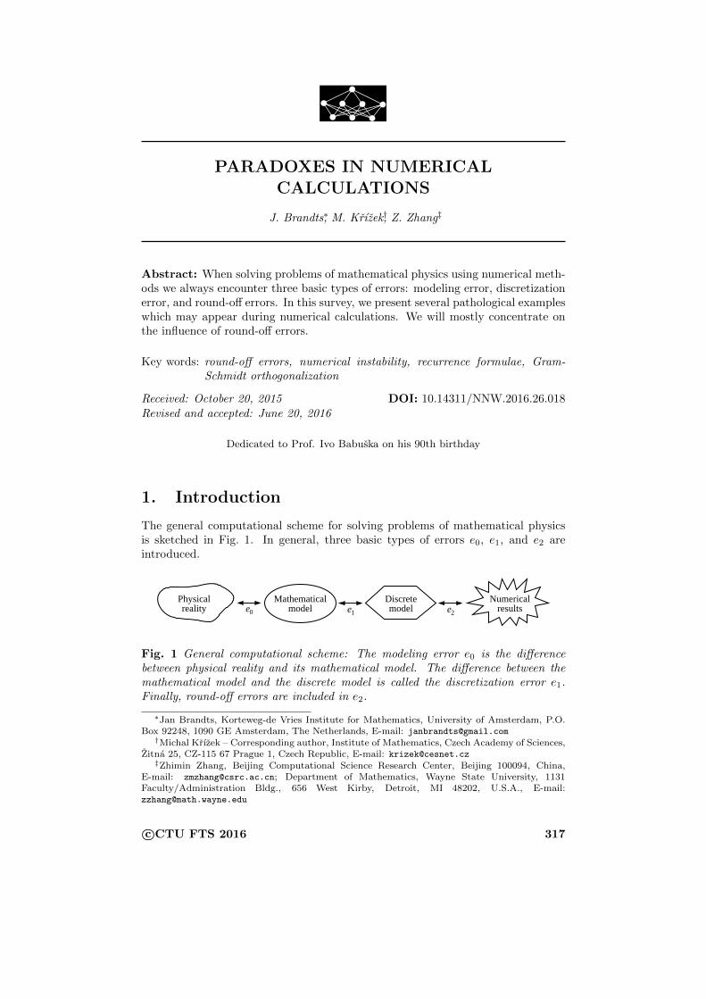
The general computational scheme for solving problems of mathematical physicsis sketched in Fig. 1. In general, three basic types of errors e0, e1, and e2 areintroduced.

results0 e1 e2

NumericalDiscreteMathematicalPhysicalreality model modele

Fig. 1 General computational scheme: The modeling error e0 is the differencebetween physical reality and its mathematical model. The difference between themathematical model and the discrete model is called the discretization error e1.Finally, round-off errors are included in e2.

∗Jan Brandts, Korteweg-de Vries Institute for Mathematics, University of Amsterdam, P.O.Box 92248, 1090 GE Amsterdam, The Netherlands, E-mail: [email protected]†Michal Krızek – Corresponding author, Institute of Mathematics, Czech Academy of Sciences,

Zitna 25, CZ-115 67 Prague 1, Czech Republic, E-mail: [email protected]‡Zhimin Zhang, Beijing Computational Science Research Center, Beijing 100094, China,

E-mail: [email protected]; Department of Mathematics, Wayne State University, 1131Faculty/Administration Bldg., 656 West Kirby, Detroit, MI 48202, U.S.A., E-mail:[email protected]

c©CTU FTS 2016 317

Neural Network World 3/2016, 317–330

We should never identify any mathematical model with reality, since no equationdescribes physical phenomena in our world exactly. This leads to the so-calledmodeling error e0.

Mathematical models are usually expressed as infinite dimensional problems.They are given by ordinary or partial differential equations, integro-differentialor integral equations, systems of these equations, variational inequalities, systemsof differential-algebraic equations, and so on. To implement such models on thecomputer we have to approximate them by finite dimensional problems, whichyields the error e1 (discretization error). This error includes for instance the errorof numerical integration, and the error of approximation of the boundary of theexamined region.

Finally, the error e2 arises during a computation in the discrete model. Itcontains, of course, rounding errors, but may include other errors (like iterationerrors).

In this paper we draw attention to hidden dangers that may appear in mechani-cal use of numerical calculations without any knowledge of theory. There is a largeamount of other works on similar topics — see e.g. [4,7–9,18,19]. Below we presentthe most drastic examples. Consider, for instance, the integral

In =1

e

∫ 1

0

xnex dx > 0.

Using integration by parts, we obtain the following recurrence relation [15, p. 505]

In = 1− nIn−1, n = 1, 2, . . . , (1)

where I0 = 1−e−1. Renata Babuskova in her 1964 paper [2] examines its numericalinstability. After a few steps of the above recurrence we surprisingly get negativevalues in single-precision arithmetic (4 bytes) even though In is positive for all n.Running the iteration in double-precision arithmetic (indicated by ˜ throughoutthis paper) on a standard PC, we observe a decreasing series until I16 = 0.0374,and then I17 = 0.3259, I18 = −5.1930 is negative, I19 = 104.8628, . . . which leadsto an alternating divergent sequence. This numerical phenomenon happens due tothe fact that at each step we subtract two numbers of almost the same size. Thenthe difference contains only a few nonzero significant digits in computer arithmeticthat necessarily leads to loss of accuracy. Note that In may be calculated via a fastconvergent series

In =1

n+ 1− 1

(n+ 1)(n+ 2)+

1

(n+ 1)(n+ 2)(n+ 3)− . . .

Similar examples are collected in the classical 1966 monograph Numerical Pro-cesses in Differential Equations [1] by Ivo Babuska, Milan Prager, and Emil Vitasek.For instance, they investigate numerical instability of successive evaluation of theexpression

. . . (((((1 : 2) · 2) : 3) · 3) : 4) · 4 . . . (2)

Their colleague Karel Segeth obtained various results for this expression on differ-ent computers involving thousands of divisions and multiplications [1, p. 6]. For

318

Brandts J., Krızek M., Zhang Z.: Paradoxes in numerical calculations

examples of large accumulations of rounding errors in calculating infinite sums orlimits see also [6, pp. 14–17].

The aim of this paper is to reveal several cautionary examples, which one shouldhave in mind before performing numerical calculations. We also recalculated threeshocking examples from a recently published monograph Handbook of Floating-Point Arithmetic [12].

2. Can a decreasing sequence be increasing in com-puter arithmetic?

Set a0 = 1, a1 = 111 , and let

an+2 =34

11an+1 −

3

11an for n = 0, 1, 2, . . . (3)

The exact solution

an =1

11n

is clearly a decreasing sequence. However, calculating (3) with MATLAB (MatrixLaboratory) on a standard PC computer, we observe that the associated seriesdecreases until a12 = 0.2068 · 10−11, then increases and reaches a40 = 40.44 andgrows quite rapidly.

This example demonstrates that subtraction of two numbers of almost the samesize is not a good practice in scientific computing. Below we list some data for (3)with different precision arithmetic,

a50 ≈ 2 · 1011 in single-precision arithmetic (4 bytes),a50 ≈ 5 · 105 in double-precision arithmetic (8 bytes),a50 ≈ 103 in extended-precision arithmetic (10 bytes).

Moreover, the corresponding sequences (an), (an), and (an) are increasing fromn = 8, 12, and 14, respectively. Rounding to two significant digits only yields anincreasing sequence from n = 2.

It is interesting to observe that if we implement (3) in a slightly different way

an+2 =34an+1 − 3an

11,

then the resulting sequence turns to be negative at a12 and remains negative after-wards with increasing magnitudes.

3. Babuska’s example

Consider the Lebesgue integrable function f on [0, 1] which is zero at all rationalnumbers and f = 1 otherwise. Then obviously∫ 1

0

f(x)dx = 1,

319


whereas any numerical quadrature formula∫ 1

0

f(x)dx ≈n∑

i=1

wif(xi)

with real weights wi and nodes xi from [0, 1] yields a zero approximate value forthis integral, since the nodes are approximated by rational numbers (with a finitenumber of decimal places).

This result, in which the numerical integration error always equals one, is dueto the fact that f is not a smooth function. Some regularity of f is usually requiredin standard theorems on convergence of quadrature formulas.

4. Kahan’s example

Set a0 = 2, a1 = −4, and consider the recurrence (see [12])

an = 111− 1130

an−1+

3000

an−1an−2for n = 2, 3, . . . (4)

Its general solution has the form

an =α100n+1 + β6n+1 + γ5n+1

α100n + β6n + γ5n,

where α, β, and γ depend on the initial values a0 and a1.Thus, if α 6= 0 then the limit of the sequence (an) is 100. Nevertheless, we

observe that if α = 0 and β 6= 0, then the limit is 6. For the initial values a0 = 2and a1 = −4 we find that

a20.= 6.034, a30

.= 6.006.

However, calculating (4) in double precision, we get

a20.= 98.351, a30

.= 99.999

due to rounding errors (cf. also [6, p. 45]).

5. Muller’s example

Let a1 = e − 1 = 1.718281828 . . . and consider the thoroughly innocent-lookingsequence (see [12])

an = n(an−1 − 1) for n = 2, 3, . . . (5)

Notice that this recurrence is only a slight modification of (1). By induction wecan easily prove that

an = n!( 1

n!+

1

(n+ 1)!+

1

(n+ 2)!+ · · ·

). (6)

320


Indeed, for n = 1 we have a1 = e−1 and assuming the validity of (6) for n−1 ≥ 0,we get by (5)

an = n(an−1 − 1) = n(

(n− 1)!( 1

(n− 1)!+

1

n!+

1

(n+ 1)!+ · · ·

)− (n− 1)!

(n− 1)!

)= n!

( 1

n!+

1

(n+ 1)!+

1

(n+ 2)!+ · · ·

).

From (6) we immediately see that the sequence (an) is decreasing, all an havea very reasonable size in the interval (1, 2), and

limn→∞

an = 1.

However, if we run the iteration on MATLAB, we observe that the sequence de-creases until a15 = 1.0668, and then a strange thing happens: a16 = 1.0685,a17 = 1.1652, a18 = 2.9731, a19 = 37.4882, a15 = 729.7637, . . . The sequencegrows out of control.

Performing only 24 subtractions and 24 multiplications in (5) with differentnumbers of significant digits, we obtain the following table:

a25 ≈ −6.204484 · 1023 in single-precision arithmetic (4 bytes),a25 ≈ 1.201807248 · 109 in double-precision arithmetic (8 bytes),a25 ≈ −7.3557319606 · 106 in extended-precision arithmetic (10 bytes).

However, by (6) we have

1.038 < 1 +1

26< a25 < 1 +

1

26+

1

262+ · · · = 26

25= 1.04,

where the standard formula for the sum of a geometric sequence was applied. Now,let us extend the number of significant digits. In arithmetic with D decimal digits,the first twelve significant digits are:

D a25(D)

20 615990.413139,

21 − 4457.98859386,

22 − 4457.98859386,

23 195.374419140,

24 40.2623187072,

25 − 6.27131142281,

26 1.48429359885.

The values corresponding D = 21 and D = 22 are the same, since the 21stdecimal digit of the Euler number e= 2.71828182845904523536028745 . . . is equalto zero. Only for D > 25 do the numerical results start to resemble the exact valuea25 = 1.03993872967 . . . For instance, if D = 30 we get a25(30) = 1.039897 . . .

321


Now let us take a closer look at the main reason of this strange behavior. Denoteby εi the rounding error at the ith step. Then we have

a1 = e− 1 + ε1 = a1 + ε1,

a2 = 2(a1 − 1) + ε2 = 2(a1 + ε1 − 1) + ε2 = a2 + 2!ε1 + ε2,

a3 = 3(a2 − 1) + ε3 = 3(a2 + 2ε1 + ε2 − 1) + ε3 = a3 + 3!ε1 + 3ε2 + ε3,

...

a25 = 25(a24 − 1) + ε25 = a25 + 25!ε1 +25!

2!ε2 +

25!

3!ε3 + · · ·+ ε25.

Therefore, the total rounding error is

a25 − a25 = −25!(ε1 +

1

2!ε2 +

1

3!ε3 + · · ·+ 1

25!ε25

)(7)

and its size depends particularly on the several initial rounding errors ε1, ε2, . . .This sophisticated example shows why it is necessary to try to avoid the subtrac-

tion of two numbers that are almost equal, which happens for instance in long-termnumerical simulations of the N -body problem (see (15) below). We observe from(7) why the above recurrence (5) is so sensitive to round-off errors. Computer arith-metic with variable length does not improve this numerical effect for large n. Aninteresting application of the sequence (5) in banking can be found in [12] and [13].

6. Rump’s example

The use of a much smaller number of subtractions than in the previous examplemay also lead to absolutely catastrophic numerical results. Evaluate the rationalfunction

u(x, y) = 333.75y6 + x2(11x2y2 − y6 − 121y4 − 2) + 5.5y8 +x

2y(8)

at x = 77617.0 and y = 33096.0. Note that this is a polynomial of degree eight plusa simple rational function x/(2y). We observe that no recurrence relation as in (5)is evaluated and we perform only three subtractions and a few other arithmeticoperations. Contrary to the previous example, we get almost the same numbers:

u(x, y) = 1.172603 in single-precision arithmetic (4 bytes),u(x, y) = 1.1726039400531 in double-precision arithmetic (8 bytes),u(x, y) = 1.172603940053178 in extended-precision arithmetic (10 bytes)

on an outmoded IMB 370 computer (see Rump [16]). The programming packageMAPLE, with

D = 7, 8, 9, 10, 12, 18, 26, 27

decimal digits produces very similar results. However, we should not rejoice overthe above results, since the exact value is

u(x, y) = −0.827396 . . . NEGATIVE!

322


As discussed in [3], for z = 333.75y6+x2(11x2y2−y6−121y4−2) and w = 5.5y8

we can evaluate exactly that

z = −7917111340668961361101134701524942850,

w = 7917111340668961361101134701524942848,

which have 35 out of 37 digits in common. Thus we are dealing with huge numberswith insufficient floating points. The exact value is

u(x, y) = z + w +x

2y= −2 +

x

2y= −54767

66192= −0.827396 . . .

Numerical results by MAPLE only begin to be realistic starting at D = 37, 38, . . .The following MATLAB code:

x = 77617.0; y = 33096.0;

y2 = y ∗ y; y4 = y2 ∗ y2; y6 = y4 ∗ y2; y8 = y4 ∗ y4; x2 = x ∗ x;

ff = 11 ∗ x2 ∗ y2− y6− 121 ∗ y4− 2;

u = 333.75 ∗ y6 + x2 ∗ ff + 5.5 ∗ y8 + x/y/2

produces u(x, y) = −1.1806E + 021, a completely false result!If we use D decimal digits in the following MATLAB code:

digits(D);

y = vpa(33096,D);

x = vpa(77617,D);

u = vpa(333.75 ∗ y 6 + x 2 ∗ (11 ∗ x 2 ∗ y 2− y 6− 121 ∗ y 4− 2) + 5.5 ∗ y 8 + x/y/2,D)

we obtain

D = 20, uD(x, y) = 1073741825.1726039401,

D = 21, uD(x, y) = 1.17260394005317863186,

D = 28, uD(x, y) = 1.172603940053178631858834905,

D = 29, uD(x, y) = −0.82739695994682136814116509548,

D = 37, uD(x, y) = −0.827396959946821368141165095479816292,

where the subscript D stands for the use of computer arithmetic with D decimaldigits. We see that when D =21 to 28, the result is close to Rump’s 1988 data,and the “correct” answer appears starting from D=29. This example shows thatthe arithmetic of large numbers should be performed very cautiously in scientificcomputing. A detailed numerical analysis of this catastrophic behavior of roundingerrors is presented in [3] and [10].

Thus, we should keep in mind that a very small number of subtractions androundings (see (5) and (8)) may completely destroy the exact solution [17]. Exam-ples showing deterministic chaos are sometimes wrongly understood, since roundingerrors were not taken into account. In many of these examples chaos appears justdue to rounding errors.

323


7. Gram-Schmidt versus Modified Gram-Schmidt

Let a1,a2,a3 ∈ Rn be linearly independent. We orthonormalize them by theGram-Schmidt (GS) process [5] and the Modified Gram-Schmidt (MGS) process.The first two vectors resulting from GS and MGS are the same, being

q1 =a1‖a1‖

and

q2 =q2

‖q2‖, where q2 = a2 − q1q

>1 a2.

Now, the difference between GS and MGS is the computation of the third vector,which in the respective cases is computed as follows,

qGS3 =

qGS3

‖qGS3 ‖

, where qGS3 = a3 − q1q

>1 a3 − q2q

>2 a3,

and

qMGS3 =

qMGS3

‖qMGS3 ‖

, where qMGS3 = (I− q2q

>2 )(I− q1q

>1 )a3.

Note that in exact arithmetic, both vectors are the same. The fundamentaldifference between MGS and GS is, that in MGS, the vector a3 is orthogonalizedagainst q1, after which the orthogonalized result is orthogonalized against q2.

To make the difference better visible, both vectors qGS3 and qMGS

3 can be com-puted in two consecutive steps as follows,

ˆqGS3 = a3 − q1(q>1 a3), qGS

3 = ˆqGS3 − q2(q>2 a3), (9)

andˆqMGS3 = a3 − q1(q>1 a3), qMGS

3 = ˆqMGS3 − q2(q>2

ˆqMGS3 ). (10)

In further steps of GS and MGS, the difference between the two methods is similar.In a practical implementation of MGS, as soon as q1 is computed, all fur-

ther vectors a2, a3, a4, . . . are orthogonalized against q1. Then, as soon as q2 iscomputed, all the vectors that resulted from the orthogonalization against q1, areorthogonalized against q2, and so on.

Example. We shall present the difference between GS and MGS in finiteprecision arithmetic. Let ε be a small number with the property that 1 + ε2 isrounded to 1 on the machine, whereas ε itself is a machine number. Let

a1 =

1εε

, a2 =

1ε0

, a3 =

10ε

be the vectors to be orthonormalized by GS and MGS. Then both GS and MGScompute the same vectors q1 and q2 as follows,

‖a1‖ =√

1 + 2ε2 ∼ 1,

324


hence q1 = a1. Next, in order to compute q2, we evaluate the inner product

q>1 a2 = 1 + ε2 ∼ 1,

and thus,

q2 = a2 − 1 · q1 =

00−ε

.Normalization can be done exactly, and thus

q2 =

00−1

.We use the two-step formula (9) above to compute ˆqGS

3 as follows:

ˆqGS3 =

10ε

− 1εε

[1 ε ε]

10ε

∼ 1

0ε

− 1εε

=

0−ε

0

,followed by

qGS3 =

0−ε

0

− 0

0−1

[0 0 − 1]

10ε

∼ 0−ε

0

− 0

0ε

=

0−ε−ε

,after which normalization gives the final result

qGS3 =

0

− 12

√2

− 12

√2

.Summarizing, the three vectors obtained by GS are

q1 =

1εε

, q2 =

00−1

, and qGS3 =

0

− 12

√2

− 12

√2

, (11)

and this is obviously far from an orthonormal basis. We observe that the thirdvector qGS

3 sweeps approximately the angle 45◦ with the plane given by q1 and q2.On the other hand, if we use the two-step formula (10) to compute the third

vector using MGS, we find

ˆqMGS3 = ˆqGS

3 =

0−ε

0

,and now the fundamentally different next step,

qMGS3 =

0−ε

0

− 0

0−1

[0 0 − 1]

0−ε

0

=

0−ε

0

,325


resulting after normalization in

qMGS3 =

0−1

0

.Thus, as the final result the three vectors

q1 =

1εε

, q2 =

00−1

, and qMGS3 =

0−1

0

.In spite of the fact that these three vectors are also not orthonormal, they aremuch closer to orthonormal than the three vectors (11) resulting from GS. Due todifferent manners of projection of round-off errors, MGS is a very helpful remedyagainst the instability of GS.

8. Eigenvalues

Consider the 3× 3 matrix

A =

1 4 2−1 1 1

1 2 1

,whose entries are small integers. Its eigenvalues can be computed by solving thecharacteristic equation det(A− λI) = 0, which reduces by Sarrus’ rule to

det(A− λI) = det

1− λ 4 2−1 1− λ 1

1 2 1− λ

= (1− λ)3 + 4− 4 + 4(1− λ)− 2(1− λ)− 2(1− λ) = (1− λ)3 = 0.

Thus, A has all three eigenvalues equal to one, just like the identity matrix. How-ever, when Matlab is used to compute these eigenvalues using the command eig(A)

the resulting values are

0.9999934375759070 and 1.000003281212047± 5.683168987282289 · 10−6i.

We see that even though the computations were performed in IEEE doubleprecision, not sixteen but only six significant digits are correct. The cause forthis is not a bug in Matlab’s software, but the inherent ill-conditioning of theeigenvalues of this particular matrix A. Indeed, suppose that a rounding errorcauses that the roots of p(x) = (1 − λ)3 + ε to be computed instead of those ofp(x) = (1 − λ)3, with ε ≈ 10−16 (see also [7, p. 17]). Then those roots are quiteclose to the numbers computed by Matlab. Thus, Matlab is doing as well as it can,given the mathematical ill-conditioning of the problem.

326


9. Numerical differentiation

Numerical differentiation represents another very instable operation. To illustrateit, consider the rational function (see [9])

g(x) =4970x− 4923

4970x2 − 9799x+ 4830, x ≥ 0.99, (12)

and calculate its second derivative at the point 1 using the second central differ-ences, i.e.

δ2hg(x) =g(1 + h)− 2g(1) + g(1− h)

h2(13)

which tends to g(1) as h→ 0. However, from the second row of Tab. I we can onlyhardly deduce which value of h is the best approximation of g(1) without knowingthat the exact value is g(1) = 94. For “large” h the function g(1 − h) quicklychanges. On the other hand, for “small” h total loss of accuracy appears, since wesubtract almost the same numbers in the nominator of (13).

δ2hg(x) h = 10−2 h = 10−3 h = 10−4 h = 10−5 h = 10−6 h = 10−7

(13) −91769.95 −2250.2 70.94 93.71 116.42 −151345(14) −91769.95 −2250.2 70.79 93.77 94.00 94.00

Tab. I Numerical values of g(1) calculated by (13) and (14), respectively.

The remedy is to rearrange formula (13) by means of (12) as follows:

δ2hg(x) =94(1− 702712h2)

(1− 712h2)(1− 702h2)(14)

which produces relatively good numerical results — see the last row of the aboveTab. I.

Finally, let us emphasize that calculation of the second derivatives from biaseddata as done e.g. in [14] is a very ill-conditioned problem.

10. The N-body problem

For an integer N ≥ 2 consider an isolated system of N mass-point bodies thatmutually interact only gravitationally. Let ri = ri(t), i ∈ {1, . . . , N}, be the so-called radius-vector in R3 describing the position of the ith body with mass mi intime t ≥ 0. Denoting the gravitational constant by G, the classical N -body problemis described by the following nonlinear system of ordinary differential equations forthe unknown trajectories ri (see [11])

ri = GN∑i6=j

mj(rj − ri)|rj − ri|3

(15)

with some initial conditions at t0 = 0 and over a time interval [0, T ] in whichit is assumed that bodies do not collide. This system is autonomous, since theright-hand side of (15) does not explicitly depend on time.

327


Can we believe numerical simulations of the evolution of the Solar system basedon (15) for billions of years in the past or future? The answer is NO from severalreasons. Newtonian mechanics does not allow any delay given by the finite speedof gravitational interaction. System (15) is only an ordinary differential equationwhose solution on the interval [0, T ] depends only on the value at point t0 = 0 andnot on the history. An extremely small modeling error ε > 0 during one year mayyield after 109 years an error of order at least ε109 which may be a quite largenumber. Also various nongravitational forces are not included in (15).

The right-hand side of (15) does not satisfy the famous Caratheodory condi-tions. Moreover, system (15) is not Lyapunov stable, i.e., extremely small changesof initial conditions or other perturbations cause very large changes in the finalstate provided the time interval is long enough. This also makes the numericalsolution unstable. Hence, the N -body problem should be treated very carefully.The above examples should be a sufficient warning.

If an integration step h gives almost the same numerical results as h/2, theintegration of the system (15) is usually stopped. However, this heuristic criterionneed not work properly. Here we present another way how to check whether ournumerical results are good. It is based on backward integration of (15) as sketchedon Fig. 2. Let r = (r1, . . . , rN ) denote a vector with 3N entries and let f = f(r)stand for the right-hand hand side of (15).

Theorem. Let r = r(t) be the unique solution of the system

r = f(r) (16)

on the interval [0, T ] with given initial conditions

r(0) = r0 and r(0) = v0. (17)

Then the function s = s(t) defined by

s(t) = r(T − t) (18)

solves the same system (16) with initial conditions s(0) = r(T ), s(0) = −r(T ) andwe have

s(T ) = r0 and s(T ) = −v0. (19)

P r o o f. According to (18) and (16), we obtain

s(t) = (−r(T − t))˙ = r(T − t) = f(r(T − t)) = f(s(t)).

We see that s satisfies the same system (16) like r. For the final conditions by (18)and (17) we get relations (19),

s(T ) = r(0) = r0 and s(T ) = −r(T − T ) = −r(0) = −v0. �

The above theorem can be applied to long-term intervals as follows. Denote byr∗ and s∗ a numerical solution of the system (15) with initial conditions (18) and

s(0) = r∗(T ) and s(0) = −r∗(T ),

328


Fig. 2 Application of the above theorem in numerical solution of the N -body prob-lem. The symbol r stands for the true solution, r∗ is the numerical solution, ands∗ is the control backward solution.

respectively. If δ > 0 is a given tolerance and

|s∗(T )− r0|+ |s∗(T ) + v0| � δ,

then it cannot hold |r(T )−r∗(T )|+|r(T )−r∗(T )| < δ, where r is the exact solution,i.e., the numerical error of the original problem (15) and (18) would be also large,as it is schematically depicted on Fig. 2.

Finally, let us point out that the previous theorem and computational strategycan be easily generalized to evolution partial differential equations.

From (15) we observe that when two bodies are close to each other (rj ≈ ri)which is an important case e.g. in space aeronautics, then we subtract in thedenominator two numbers of almost the same size. This may lead to a catastrophicloss of accuracy.

11. Conclusions

In computer arithmetic, only a finite number of significant digits is used. This factmay lead to a catastrophic loss of accuracy, in particular, when numerical schemesare not stable. The aim of this paper was to present several thoroughly innocent-looking examples that produce completely nonsensical results. They are of severaltypes “in limit”:

1) the expression in (2) is of type 1∞,2) the right-hand side of (8) is of type ∞−∞,3) the fraction in (13) is of type 0/0,4) the product in (5) is of type 0 · ∞.In preforming any real-life calculations in noninteger computer arithmetic, we

should keep in mind that we always produce three basic kinds of errors: modelingerror, discretization error, and rounding errors. They usually grow exponentiallywith time. Hence, we should very carefully and critically evaluate the numericaloutput and should not blindly trust computer results as it is often done.

Acknowledgement

The authors would like to thank L’ubomıra Balkova, Jan Chleboun, Edita Pelan-tova, Lawrence Somer, and Tomas Vejchodsky for useful discussions and extensive

329


calculations. The second author was supported by Grant no. P101/14-02067S andRVO 67985840. The research of the third author was supported in part by theNational Natural Science Foundation of China under grants 11471031, 91430216,and the U.S. National Science Foundation through grant DMS-1419040.

References

[1] BABUSKA I., PRAGER M., VITASEK E. Numerical processes in differential equations.John Willey & Sons, London, New York, Sydney, 1966.

[2] BABUSKOVA R. Uber numerische Stabilitat einiger Rekursionsformeln. Apl. Mat. 1964, 9,pp. 186–193.

[3] CUYT A., VERDONK B., BECUWE S., KUTERNA P. A remarkable example ofcatastrophic cancellation unraveled. Computing 2011, 66, pp. 309–320, doi: 10.1007/

s006070170028.

[4] FORSYTHE G.E. Pitfalls in computation, or why a math book isn’t enough. Amer. Math.Monthly 1970, 77, pp. 931–956, doi: 10.2307/2318109.

[5] HAZEWINKEL M. (ed.) Orthogonalization. Springer, 2001.

[6] HIGHAM N. J. Accuracy and stability of numerical algorithms. SIAM, Philadelphia, 2002.

[7] KRIZEK M., PRAGER M., VITASEK E. Reliability of numerical calculations. PokrokyMat. Fyz. Astronom. 1997, 42(2), pp. 8–23. In Czech.

[8] KRIZEK M., ZHANG Z. Reliability of numerical calculations. Math. Culture 2015, 6(1), pp.34–40. In Chinese.

[9] KULISH U., MIRANKER W. L. The arithmetic of the digital computer: a new approach.SIAM Rev. 1986, 28(1), pp. 1–40, doi: 10.1137/1028001.

[10] LOH E., WALSTER G. W. Rump’s example revisited. Reliable Comput. 2002, 8, pp. 245–248.

[11] MARCHAL C. The three-body problem. Elsevier, Amsterdam, 1991.

[12] MULLER J.-M. et al. Handbook of floating-point arithmetic. Birkhauser, 2009.

[13] PELANTOVA E., ZNOJIL M. Can we believe our own calculator? Rozhledy mat.-fyz. 2010,85, pp. 11–18. In Czech.

[14] PERLMUTTER S. Supernovae, dark energy, and the accelerating universe. Physics Today2003, 56, April, pp. 53–60, doi: 10.1063/1.1580050.

[15] REKTORYS K. Survey of applicable mathematics I. Kluwer Acad. Publ., Dordrecht, 1994.

[16] RUMP S.M. Algorithms for verified inclusions — theory and practice. In: Reliability inComputation (ed. R. E. Moore), Academic Press, New York, 1988, pp. 109–126.

[17] RUMP S.M. Verification methods: Rigorous results using floating-point arithmetic. ActaNumerica 2010, 19, pp. 287–449, doi: 10.1017/S096249291000005X.

[18] STEGUN I.A., ABRAMOWITZ M. Pitfalls in computation. J. Soc. Indust. Appl. Math.1956, 4(4), pp. 207–219.

[19] WILKINSON J.H. Rounding errors in algebraic processes. Prentice-Hall, New York, 1963.

330

http://dx.doi.org/10.1007/s006070170028

http://dx.doi.org/10.1007/s006070170028

http://dx.doi.org/10.2307/2318109

http://dx.doi.org/10.1137/1028001

http://dx.doi.org/10.1063/1.1580050

http://dx.doi.org/10.1017/S096249291000005X

paradoxes in numerical calculations - … arises during a computation in the discrete model. it ......

Documents