paper75 space syntax

8/3/2019 Paper75 Space Syntax

http://slidepdf.com/reader/full/paper75-space-syntax 1/36

UCL CENTRE FOR ADVANCED SPATIAL ANALYSIS

WORKINGPAPERS

SERIESPaper 75 - Mar 04

A New Theory of Space

Syntax

ISSN 1467-1298



A New Theory of Space Syntax1

Michael [email protected]

Centre for Advanced Spatial Analysis, University College London,

1-19 Torrington Place, London WC1E 6BT, UK

http://www.casa.ucl.ac.uk/

February 23, 2004

Abstract

Relations between different components of urban structure are often measured in a

literal manner, along streets for example, the usual representation being routes

between junctions which form the nodes of an equivalent planar graph. A popular

variant on this theme – space syntax – treats these routes as streets containing one or

more junctions, with the equivalent graph representation being more abstract, based

on relations between the streets which themselves are treated as nodes. In this paper,

we articulate space syntax as a specific case of relations between any two sets, in this

case, streets and their junctions, from which we derive two related representations.

The first or primal problem is traditional space syntax based on relations between

streets through their junctions; the second or dual problem is the more usualmorphological representation of relations between junctions through their streets.

The unifying framework that we propose suggests we shift our focus from the primal

problem where accessibility or distance is associated with lines or streets, to the dual

problem where accessibility is associated with points or junctions. This traditional

representation of accessibility between points rather than between lines is easier to

understand and makes more sense visually. Our unifying framework enables us to

easily shift from the primal problem to the dual and back, thus providing a much

richer interpretation of the syntax. We develop an appropriate algebra which provides

a clearer approach to connectivity and distance in the equivalent graph

representations, and we then demonstrate these variants for the primal and dual

problems in one of the first space syntax street network examples, the French villageof Gassin. An immediate consequence of our analysis is that we show how the direct

connectivity of streets (or junctions) to one another is highly correlated with the

distance measures used. This suggests that a simplified form of syntax can be

operationalized through counts of streets and junctions in the original street network.



1

1 Traditional Representations

Urban form is usually represented as a pattern of identifiable urban elements such as

locations or areas whose relationships to one another are often associated with linear

transport routes such as streets within cities. These elements can be thought of as

forming nodes in a graph, the relations between the nodes being arcs which represent

direct flows or associations between the elements. These need not be physically

rooted in the detailed geometry of buildings for they might be more abstract such as

migration flows between regions but at more local levels, they are usually taken to be

linear features such as streets or corridors. The focus of such analysis is on the

relative proximity or ‘accessibility’ between locations which involves calculating

distances between nodes in such graphs and associating these with densities and

intensities of activity which occur at different locations and along the links between

them. For example, clusters of work activity are usually associated with high levels of

accessibility. Much planning and design is concerned with changing the patterns of

such accessibility through the development of new transport infrastructures.

There is a long tradition of research articulating urban form using graph-theoretic

principles. Nystuen and Dacey (1961) developed such representations as measures of

hierarchy in regional central place systems, while Kansky (1963) applied basic graph

theory to the measurement of transportation networks. Graphs are implicit in the

definition of gravitational potential based on the weighted sum of forces around a

point first applied to population systems by Stewart (1947), and subsequent work on

identifying accessibility as a key determinant of spatial interaction is based on an

implicit graph-theoretic view of spatial systems (Hansen, 1959; Wilson, 1970). The

widespread use of network analysis in geographic science reviewed by Haggett and

Chorley (1969) establishes such analysis as central to spatial analysis. In a similar

manner, graphs have been widely used to represent the connectivity between rooms in

buildings (March and Steadman, 1971) and to classify different building types

(Steadman, 1983). They have long been regarded as the basic structures for

representing forms where topological relations are firmly embedded within Euclidean

space.



2

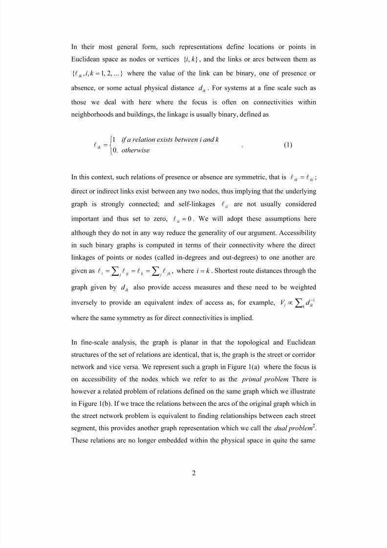
In their most general form, such representations define locations or points in

Euclidean space as nodes or vertices , k i , and the links or arcs between them as

...,2,1,, =k iik l where the value of the link can be binary, one of presence or

absence, or some actual physical distance ik d . For systems at a fine scale such as

those we deal with here where the focus is often on connectivities within

neighborhoods and buildings, the linkage is usually binary, defined as

=otherwise ,

and k between iion existsif a relat ik

0

1l . (1)

In this context, such relations of presence or absence are symmetric, that is kiik ll = ;

direct or indirect links exist between any two nodes, thus implying that the underlying

graph is strongly connected; and self-linkages iil are not usually considered

important and thus set to zero, 0=iil . We will adopt these assumptions here

although they do not in any way reduce the generality of our argument. Accessibility

in such binary graphs is computed in terms of their connectivity where the direct

linkages of points or nodes (called in-degrees and out-degrees) to one another are

given as ,∑∑ === j jk k j iji llll where k i = . Shortest route distances through the

graph given by ik d also provide access measures and these need to be weighted

inversely to provide an equivalent index of access as, for example, ∑ −∝k ik i d V 1

where the same symmetry as for direct connectivities is implied.

In fine-scale analysis, the graph is planar in that the topological and Euclidean

structures of the set of relations are identical, that is, the graph is the street or corridor

network and vice versa. We represent such a graph in Figure 1(a) where the focus is

on accessibility of the nodes which we refer to as the primal problem. There is

however a related problem of relations defined on the same graph which we illustrate

in Figure 1(b). If we trace the relations between the arcs of the original graph which in

the street network problem is equivalent to finding relationships between each street

segment, this provides another graph representation which we call the dual problem2.

These relations are no longer embedded within the physical space in quite the same



3

way as the initial links for they now represent abstract relations between streets. These

are relations through the joining of streets at junctions whereas the primal problem is

posed as relations between junctions where the links are the streets themselves.

a. The Planar Graph as Primal

b. The Dual of the Planar Graph

Figure 1: Conventional Graph-Theoretic Representation of the Street Network

This dual problem has not found great favor in spatial analysis. The focus on linear

features rather than locations has rarely been developed for the dual privileges lines or streets as the objects of interest, rather than locations or street junctions. Moreover the

dual breaks the clear link between Euclidean and topological space and this makes

visual analysis of the dual more difficult. Nevertheless there is a tradition where this

dual has been widely developed and this is space syntax (Hillier and Hanson, 1984).

The theory has its roots in quite sophisticated speculation that the evolution of built

form can be explained in analogy to the way biological forms unravel (Hillier,

Leaman, Stansall, and Bedford, 1976). In its current and widely applied form

however, it is more a toolbox of simple techniques for measuring street accessibilityin towns and associating this with movement and lines of sight (Hillier, Penn, Hanson,

Grajewski, and Xu, 1993). But the key characteristic in space syntax is that

precedence is given to linear features such as streets in contrast to fixed points which

approximate locations (Hillier, 1996).



4

Figure 1 in fact illustrates that there is a clear path between the primal and dual

problems which has rarely been mapped out, certainly not within space syntax. This

paper will establish a unifying framework so that one can easily move between the

primal and dual problems and in this way show how space syntax can be translated

into a more familiar locational analytic frame. We need to explain space syntax first

and we will do this in the next section but then we will establish our unifying

framework showing how connectivity and distance in both the primal and dual

problems can be more easily understood. We then illustrate how spatial averaging is

involved in computing accessibility and present all these results for the primal and

dual problems for the original example – the French village of Gassin – first

introduced by Hillier and Hanson (1984). We show how the ability to move from one

problem to its dual enables a much more satisfactory visual analysis, showing finally

how we might add distance back into space syntax. Here we both simplify space

syntax and produce a simplified version while pointing the way to further

generalization of the problem and its relation to current developments in the

evolutionary and statistical theory of networks (Dorogovtsev and Mendes, 2003)

2 Explaining Space Syntax

In space syntax, the focus is on lines not points, streets not the junctions that anchor

them as we illustrated in Figure 1. This is not particularly controversial although it is

often difficult to approximate a street by a centroid but where the analysis departs

from the dual formulation in Figure 1(b) is that the map is no longer planar: street

segments do not have to be anchored by nodes at two ends for a street can have any

number of nodes greater than or equal to one. Streets are very definitely not locations

in this interpretation and thus the relations between any two streets can never be

uniquely embedded in Euclidean space. This makes the analysis of the topological

relations between streets entirely abstract; it forces the representation of distance

between two streets to be distance in the graph-theoretic rather than the Euclidean

sense, thus removing the relational graph from the physical space in which it is

defined in the first instance.



5

In Figure 2(a), we show how the simple graph from Figure 1(a) can be relabeled to

generate a different relational structure in which arcs have one or more nodes

associated with them which is the essence of space syntax representation. The new

street graph is not planar, and thus it is not appropriate to refer to this as a graph any

longer. It is usually called an axial map and the lines that compose it are called axial

lines. There is some controversy about how such lines are defined but a general

consensus seems to be that these are ‘lines of sight’ rather than lines of unobstructed

movement. This tends to limit space syntax to the urban design scale where streets

rather than generic transport routes are important and where detailed urban

morphology and geometry is the focus. In Figure 2(b), we show the space syntax

graph which is defined by associating any two streets if they have a junction/node in

common. There is an immediate and clear difference from the planar graph: that is, a

street increases in importance as the number of nodes associated with it gets greater.

In terms of the traditional problem, the importance of a node increases the greater the

number of lines or streets associated with it but the dual of this primal is different

from the primal of the space syntax problem as we will show below.

a. The Street Network as an Axial Map

b. The Primal Syntaxbetween Streets/Lines

c. The Dual Syntaxbetween Junctions/Points

Figure 2: Space Syntax Representation



6

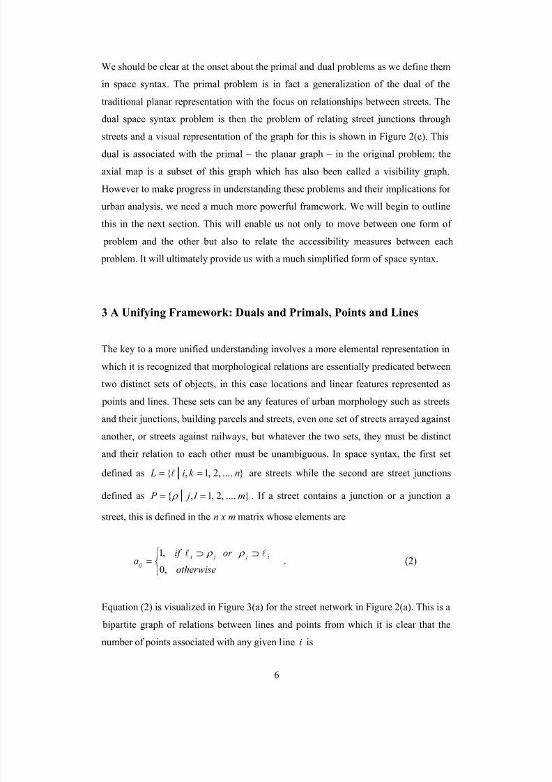
We should be clear at the onset about the primal and dual problems as we define them

in space syntax. The primal problem is in fact a generalization of the dual of the

traditional planar representation with the focus on relationships between streets. The

dual space syntax problem is then the problem of relating street junctions through

streets and a visual representation of the graph for this is shown in Figure 2(c). This

dual is associated with the primal – the planar graph – in the original problem; the

axial map is a subset of this graph which has also been called a visibility graph.

However to make progress in understanding these problems and their implications for

urban analysis, we need a much more powerful framework. We will begin to outline

this in the next section. This will enable us not only to move between one form of

problem and the other but also to relate the accessibility measures between each

problem. It will ultimately provide us with a much simplified form of space syntax.

3 A Unifying Framework: Duals and Primals, Points and Lines

The key to a more unified understanding involves a more elemental representation in

which it is recognized that morphological relations are essentially predicated between

two distinct sets of objects, in this case locations and linear features represented as

points and lines. These sets can be any features of urban morphology such as streets

and their junctions, building parcels and streets, even one set of streets arrayed against

another, or streets against railways, but whatever the two sets, they must be distinct

and their relation to each other must be unambiguous. In space syntax, the first set

defined as ....,2,1, nk i L == l are streets while the second are street junctions

defined as ....,2,1, ml j P == ρ . If a street contains a junction or a junction a

street, this is defined in the n x m matrix whose elements are

⊃⊃

=otherwise

or if a

i j ji

ij,0

,1 ll ρ ρ . (2)

Equation (2) is visualized in Figure 3(a) for the street network in Figure 2(a). This is a

bipartite graph of relations between lines and points from which it is clear that the

number of points associated with any given line i is



7

∑=

=m

j

iji a1

l , (3)

and the number of lines associated with any point j

∑=

=n

i

ij j a1

ρ . (4)

Equations (3) and (4) define the respective in-degrees and out-degrees of the

associated graph. In the sequel, we will drop the full range of summation for this will

be the same for every such operation.

a. The Data as a Bipartite Graph

b. The Primal Syntax betweenStreets/Lines

c. The Dual Syntax between Junctions/Points

Figure 3: Space Syntax as Bipartite Graphs

The primal-dual nature of this representation is already implied in the line-point

asymmetry and the direct connectivity indices for lines and points in equations (3) and

(4). As we shall see, lines are not privileged over points or vice versa. In fact, the

planar graph and space syntax representations are particular cases within the

framework, and these can be compared quite easily. Noting that for the planar graph

case, the number of points for each line is always fixed at ii ∀= ,2l (as each street

segment has a node at its beginning and end), then a measure of the deviation from



8

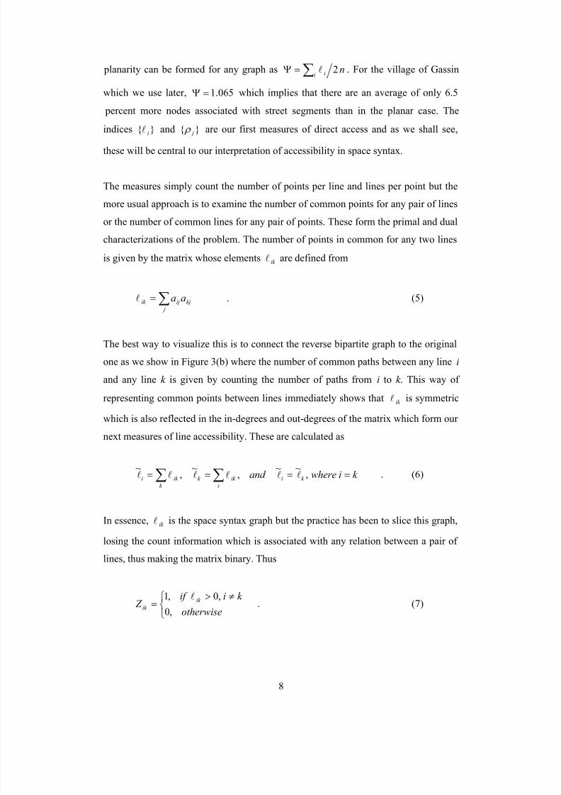
planarity can be formed for any graph as ni i 2∑=Ψ l . For the village of Gassin

which we use later, 065.1=Ψ which implies that there are an average of only 6.5

percent more nodes associated with street segments than in the planar case. The

indices il and j ρ are our first measures of direct access and as we shall see,

these will be central to our interpretation of accessibility in space syntax.

The measures simply count the number of points per line and lines per point but the

more usual approach is to examine the number of common points for any pair of lines

or the number of common lines for any pair of points. These form the primal and dual

characterizations of the problem. The number of points in common for any two lines

is given by the matrix whose elements ik l are defined from

∑= j

kjijik aal . (5)

The best way to visualize this is to connect the reverse bipartite graph to the original

one as we show in Figure 3(b) where the number of common paths between any line i

and any line k is given by counting the number of paths from i to k . This way of

representing common points between lines immediately shows that ik l is symmetric

which is also reflected in the in-degrees and out-degrees of the matrix which form our

next measures of line accessibility. These are calculated as

∑ ∑ ====k

k i

i

ik k ik i k iwhereand ,~~

,~

,~

llllll . (6)

In essence, ik l is the space syntax graph but the practice has been to slice this graph,

losing the count information which is associated with any relation between a pair of

lines, thus making the matrix binary. Thus

≠>

=otherwise

k iif Z

ik

ik ,0

,0,1 l. (7)



9

Note that the slicing in equation (7) also loses information about the strength of the

self-loops. In fact we consider that this type of slicing is unnecessary for valuable

information about the strength of relations is lost and we suggest that space syntax

practitioners henceforth work with ik l rather than ik Z . However we consider that this

is a detail which does not make a substantial difference to the ensuing analysis.

The dual problem follows directly and can be stated in analogous manner. First the

number of lines common to any two points can be calculated as

∑=i

il ij jl aa ρ , (8)

and the measures of direct access or connectivity in the graph based on in-degrees and

out-degrees are given as

∑ ∑ ====l

l j

j

jl l jl j l jwhereand ,~~,~,~ ρ ρ ρ ρ ρ ρ . (9)

The equivalent bivariate graph representation is illustrated in Figure 3(c) where it is

clear that the matrix ][ jl ρ is symmetric and counts the number of paths between any

pair of points in terms of their common lines.

The primal and dual problems interlock with one another in an intriguing way which

has direct practical implications for how point accessibility can be translated into line

accessibility and vice versa. To demonstrate this, we need to shift to matrix notation

which provides a much more parsimonious form for laying bare the nature of this

interlocking. We will define all matrices and vectors in bold upper and lower case

type respectively, starting from the basic n x m matrix of relations ][ ija=A . We will

transpose this matrix asT

A but where we need to sum the elements of such matrices

using the unit vector 1 , we will not make any distinctions in terms of the transpose

operation: use will be clear from context. We can now state the primal (space syntax)

problem from equations (3), (5) and (6) as



10

1LAAL1A === ll~

,, and T , (10)

from which it is clear that L and l~

are symmetric:T T T T

AAAALL === )( , and

1LAA1L1 === T T T T )(~l . The dual problem has a similar structure

P1AAPA1 === ρ ρ ~,, and T , (11)

with analogous symmetries. The relation between the two problems is easy to

illustrate. In equation (11) if we post-multiply A1= ρ byT

A , we derive

T A ρ =l

~(12)

and if we pre-multiply 1A=l by T A , we get

lT T A= ρ ~ . (13)

The meaning of these relations is slightly tortuous; the number of common points for

each pair of lines in equation (12) can be seen as a convolution of the number of lines

for each point with respect to the existence of any line at each point. The number of

common lines for each pair of points has an analogous interpretation.

In fact ρ ρ ~and,,~

, ll will be the key indices of direct accessibility/connectivity

which we will use and compare in the sequel but before we broach the whole subject

of distance in the graphs of these primal and dual problems, we must note the origins

of the approach. The idea of interpreting relations between two sets in the field of

urban analysis is due to Atkin (1971) who pioneered ‘Q-analysis’. This analysis

begins with relations arrayed in the form of the matrix A with dual and primal

characterizations similar to those here, but being represented in a geometry called a

simplicial complex (the primal) and its conjugate (the dual). Q-analysis was never

widely exploited, perhaps because of its rather arcane presentation, and it was rarely

linked to the theory of graphs. From a rather different perspective, this kind of primal-



11

dual framework was exploited by Coleman (1971) in his interpretation of social

exchange, it was generalized and linked to graph theory by Batty and Tinkler (1979),

and related to social power in design-decision-making by Batty (1981). Until quite

recently, the framework has only occasionally been exploited but it has been

rediscovered in the great wave of recent interest in networks, their evolution and their

statistics. It is currently being widely exploited in the analysis of social networks

using small worlds by Watts (2003) and Newman (2003). There have been some

attempts at examining alternative graph-theoretic relations in space syntax itself (see

Kruger, 1989) and Jiang and Claramunt (2000) have suggested that the visibility

graph, which is in essence the graph of the dual, be the subject of analysis, shifting the

focus to points rather than lines, as we suggest in this paper.

4 Patterns in the Syntax: Connectivity and Distance

The connectivity measures introduced above are measures of direct access to lines and

points from the same elements that are immediately adjacent to them, that link with

them directly. More appropriate measures of distance although taking account of such

adjacency are based on indirect links between the system elements. The usual form is

to calculate shortest routes between the elements, thence computing the associated in-

degrees and out-degrees which provide measures of potential or accessibility. In this

section, we will introduce the standard measure and then propose another which has

more desirable features but in each case, these distances will be based on the

interaction matrices L for lines and P for points. We will first illustrate our standard

measure for the primal problem where we start with the matrix L which gives the

number of points which are common between any pair of lines. What we require is a

computation of the number of common points between all paths in the graph that exist

between any two lines which are at different steps removed from one another. The

elements of the basic matrix ik l are one step removed from each other and are direct

links while the number of two-step paths is given by

∑= z

zk iz ik lll12 , (14)



12

where 1

ik l is the basic matrix element ik l . Successive numbers of paths of length s

are thence computed as

∑=+

z

zk

s

iz

s

ik lll1 . (15)

We compute a measure of distance however not in terms of the number of points

associated with these path lengths but in terms of the actual path length which

minimizes the distance between any two lines i and k . Thus formally

sd thenand if ik

s

ik

s

ik ==>+)(,001

lll (16)

where s is the length of the path. In a strongly connected graph (which all graphs

here are by definition), 0)( >ik d l when the path length s reaches n , if not before.

This is a standard result of elementary matrix algebra and equations (15) and (16) thus

provide the algorithm which enables shortest paths in these kinds of graph to be

computed.

We noted earlier that in space syntax, the matrix that is used is not ][ ik l but its binary

form ][ ik Z defined in equation (7). However this gives a distance matrix very close

to ])([ ik d l . The weighting produced by raising L to successive powers which is what

the algorithm in essence is doing, is of no relevance. In fact even though the matrix

][ ik Z has its self-elements 0=ik Z , the two-step paths become positive, and the

resulting distance matrix is highly correlated with that produced by the process in

equations (15) and (16). It is however easier to present these operations using matrix

notation. Thus for the primal problem, successive powers of L are given by

LLL

s s =+1

. The distance matrix which we now write as )(l

D becomes stable whenn s ≤ . An exactly analogous process is used to generate the dual distance matrix

where the point to point matrix P which gives the number of common lines between

any pair of points, is raised to successive powers PPP s s =+1 with the distance

matrix computed as )( ρ D .



13

We compute the in-degrees (and out-degrees but these are the same because of

symmetry) of successive powers of the appropriate matrices as

s s s s and P11L == ρ ~~l , (17)

and there are multiple ways of showing how these in-degree vectors for the primal

and dual problems interlock with one another. We state without further explanation

the nature of this interlocking for each problem as

===

===−−−

−−−

ALPP

PALL

111

111

~~

~~~

sT s s s

T s s s s

l

lll

ρ ρ ρ

ρ . (18)

The relationships in equations (17) and (18) provide a wealth of alternate

interpretations for the meaning of path length in graphs of this nature. Further analysis

along these lines however takes us away from the focus of this paper and must await

future work.

The aggregate distances from a line to all others in the primal problem and from a

point to all others in the dual are computed in the usual way by summing the relevant

distance matrices as in-degrees or out-degrees, that is

)()()()( ρ ρ P1d1Dd == and ll . (19)

In fact these distances are measures of inaccessibility rather than accessibility and

need to be inverted in some way to provide appropriate measures. In space syntax,

)(ld is referred to as depth and is usually averaged with respect to the number of

lines in the system n . This is necessary if lines (and zones of lines) within a certain

distance or depth from a given line are to be identified but it makes no difference to

the relative distribution. The measure of access used in space syntax simply takes the

mean values of distance for the primal problem and inverts each, providing an index

which is called ‘integration’. Variations in these indices exist (Teklenberg,

Timmermans, and Wagenberg, 1993) but for the primal and the dual, integration (or

accessibility) for each element is usually defined as



14

])([

1)(

])([

1)(

md d and

nd d

j

j

i

i ρ

ρ ==l

l . (20)

The main problem with these measures is that they ignore both the relative

importance and the strengths of paths through the graph. First information is lost

through the fact that connectivity strengths are transformed to simple step-length

distances as in equation (16). Second, each step is given equal weight whereas it

might be assumed that as the step length gets greater, the relative importance of the

step gets smaller. Third, the number of steps in the graph depends upon the size of the

graph and thus systems of different sizes cannot be compared. Some normalization

has to take place to ensure comparison. Some of these issues have been tackled but

they are best resolved with a new measure of distance that relies on the basic path

connectivity matrices L and P and on some notion that larger step lengths act like

distances in Euclidean space, becoming increasingly less important.

There are many possibilities and we simply introduce one of these here. For the line to

line interaction matrix ][ ik l , we weight each matrix power s by sω and form the

linear combination

∑= s

s

ik

s

ik D ll ω )(~

(21)

where sω declines with increasing path length s . If we set this weight as sλ where s

is now a power (as well as an index) and 10 << λ , then as ∞→ s , 0→ sλ . The

aggregate distance for line i can be computed as

∑ ∑ ∑∑ === s k s

si

s sik

s

k

ik i Dd llll ~)(~)(~ λ λ . (22)

We can fix the range of the summation over s is to a value determined by the size of

sλ . When s is the size of the matrix, all step-lengths are guaranteed to be positive and



15

1<<nλ but usually the range can be fixed at the point s where all the step lengths

become positive. The equivalent measure for the dual problem is defined as

∑=

s

s

j

s

jd ρ λ ρ ~)(~

. (23)

This definition illustrates that each path length makes a specific contribution to the

overall definition of distance and this can be tuned by fixing the value of λ . In the

Gassin example, we fix 05.0=λ . If we then measure the contribution of each path

length s for the primal (line) problem as ∑∑=Φiks

s

ik ik

s

ik ll , we generate the

following proportions of activity: 717.0,1 =Φ= s ; 178.0,2 =Φ= s ;

062.0,3 =Φ= s ; 025.0,4 =Φ= s ; and 019.0,5 =Φ= s , where the maximum

path length (or depth) between streets in the Gassin axial map is 5.

We now have four measures of accessibility for each of the two problems: two based

on direct or adjacent distances and two based on all distances. For the primal problem

these are the vectors ,l ,~l )(dl and )(

~ld , for the dual , ρ ,~ ρ )(d ρ and )(

~ ρ d . What

we suspect in space syntax graphs where the average depth or step-length is small – in

Gassin it is 3.239 – is that these measures are highly correlated with one another. To

test this hypothesis, we have examined 1000 randomly constructed systems of points

and lines where the number of lines varies from 30 to 60 and points varies from 40 to

80. We also vary the density of relations between lines and points measured using the

ratio of the total number of relations to the potential number, ])(1[ nmaij ij∑−=Θ ,

from 0.75 to 0.99. Note that in Gassin, the number of lines is 41, the number of points

63, and the ratio 948.0=Θ so these randomized runs are comparable with our real

case. Because we have ruled out all disconnected systems from these random runs, the

average density is 825.0=Θ , the average number of lines 45 and the average number

of points 59. The systems generated are somewhat dense axial maps with an average

step length of around 2.6. As such these provide a coarse first attempt at comparing

various types of distances measures but we require much further work to support the

tentative conclusions we draw here. We define an index of similarity between each

pair of distances which we just show for the example of l and l~

as



16

∑∑

∑∑

−

−=Ξ

k

k i

k

k i

k

k i

)(

)~~

()(

1)~

:(ll

llll

ll . (24)

This measure is chi-square-like and varies between 1 – complete similarity, and 0 –

complete dissimilarity. The other measures are computed accordingly for both the

primal and dual problems.

(a) Line Distances l l~

)(dl )(~

ld

l • 0.927 0.775 0.914

l~

(0.030) • 0.767 0.972

)(dl (0.069) (0.082) • 0.769

)(~ ld (0.041) (0.020) (0.049)•

(b) Point Distances ρ ρ ~ )(d ρ )(~ ρ d

ρ • 0.898 0.638 0.880

ρ ~ (0.048) • 0.626 0.959

)(d ρ (0.163) (0.178) • 0.687

)(~ ρ d (0.064) (0.031) (0.117) •

Table 1: Average Similarities Ξ between the Four Distance Measures

(The comparisons are symmetric and the statistics in brackets below the diagonal are standard

deviations of the relevant similarity measure above the diagonal).

Comparisons of these distance measures are shown in Tables 1(a) and (b) for the

primal and dual problems respectively. Three of the distance measures based on the

in-degrees and out-degrees of the original data matrix A , the basic interaction

matrices L and P , and the weighted distance matrices )(~

lD and )(~ ρ D are more than

80 percent similar to one another. The step-length distance matrix )(lD has around 70

percent similarity with these other three measures while the matrix )( ρ D has only 60

percent similarity. Nevertheless this suggests that the direct measures of access which

ignore all indirect links, are quite good measures of the importance of lines or points

in the primal or dual problems where the axial map is quite densely connected which

these 1000 runs imply. As we shall see, these results are similar to the Gassin example

reported below although there is considerable volatility in the similarities between l~



17

and )(ld , and ρ ~ and )( ρ d which are revealed in Figure 4. This suggests that where

we have more points than lines as in many space syntax problems, then it is amongst

the points that the greatest discrimination with respect to accessibility occurs. This

might seem counter-intuitive for space syntax privileges lines over points, streets over

their junctions, yet there is a sense in any problem where one set is numerically

greater in its mass than another, that this set will have greater significance. We will

return to this in our analysis of Gassin below, but before we do so, we need to

introduce one last idea about the meaning of distance.

(a) Similarity between l~

and )(dl (a) Similarity between ρ ~ and )(d ρ

Figure 4: Variations in Similarity between Direct Distanceand Indirect Step-Distance

5 The Algebra of Syntax: Averaging Lines into Points and Points into

Lines

It makes sense to explore whether or not there are distance vectors associated with the

relative accessibility between lines which can be derived by consistently weighting

the points and vice versa. This would amount to a perfect interlocking of the primaland dual problems but it would also provide a form of natural averaging between lines

and points. In short, what we require are vectors ][ il and ][ j ρ such that

∑=i

iji j X l ρ , and (25)



18

∑= j

ij ji Y ρ l , (26)

where the matrices ][ ij X and ][ ijY give the respective weights of each point in each

line and each line as part of each point. Equations (25) and (26) can thus be regarded

as types of steady state equation.

The problem must be grounded of course in data which somehow relates to the

structural matrix ][ ij A with an obvious definition of these weights given as follows.

We first express the relative importance of each point j to a given line i as

∑=l

il

ij

ij A

A

X , ∑ = jij X 1 , (27)

and the relative importance of each line i to a given point j as

∑=

k

kj

ij

ij A

AY , ∑ =

i

ijY 1 . (28)

The problem is now well defined. We seek vectors ρ and l which are solutions to

equations (25) and (26) respectively which in matrix terms are Xl= ρ and Y ρ =l .

There are two ways of proceeding. First simple substitution of equations (25) into (26)

and (26) into (25) leads to

∑∑=i l

ijil l j X Y ρ ρ , and (29)

ij

j k

kjk i Y X ∑∑= ll . (30)

The matrix weightings in equations (29) and (30) can be defined as



19

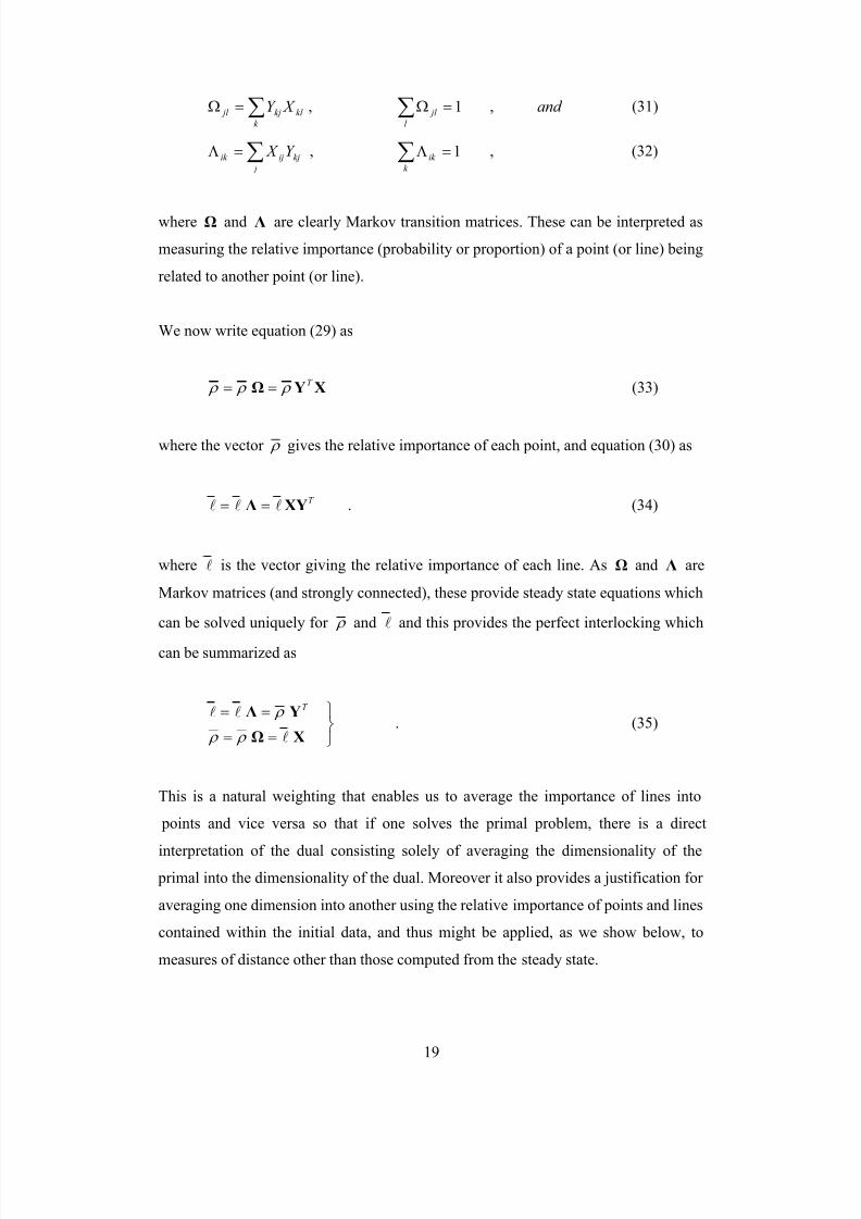
∑=Ωk

kl kj jl X Y , ∑ =Ωl

jl 1 , and (31)

∑=Λ j

kjijik Y X , ∑ =Λk

ik 1 , (32)

where Ω and Λ are clearly Markov transition matrices. These can be interpreted as

measuring the relative importance (probability or proportion) of a point (or line) being

related to another point (or line).

We now write equation (29) as

XYΩT

ρ ρ ρ == (33)

where the vector ρ gives the relative importance of each point, and equation (30) as

T XYΛ lll == . (34)

where l is the vector giving the relative importance of each line. As Ω and Λ are

Markov matrices (and strongly connected), these provide steady state equations which

can be solved uniquely for ρ and l and this provides the perfect interlocking which

can be summarized as

==

==

XΩ

YΛ

l

ll

ρ ρ

ρ T

. (35)

This is a natural weighting that enables us to average the importance of lines into

points and vice versa so that if one solves the primal problem, there is a direct

interpretation of the dual consisting solely of averaging the dimensionality of the primal into the dimensionality of the dual. Moreover it also provides a justification for

averaging one dimension into another using the relative importance of points and lines

contained within the initial data, and thus might be applied, as we show below, to

measures of distance other than those computed from the steady state.



20

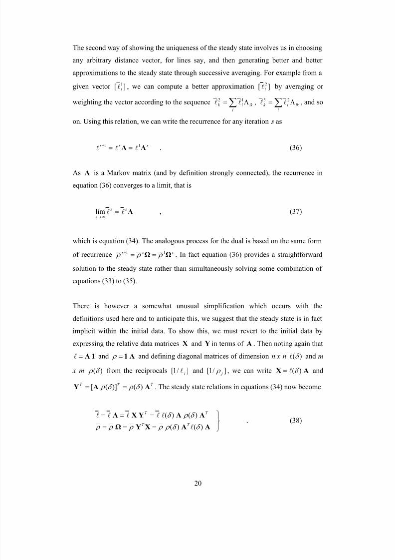
The second way of showing the uniqueness of the steady state involves us in choosing

any arbitrary distance vector, for lines say, and then generating better and better

approximations to the steady state through successive averaging. For example from a

given vector ][ 1

il , we can compute a better approximation ][ 2

il by averaging or

weighting the vector according to the sequence ik

i

ik Λ= ∑12

ll , ik

i

ik Λ= ∑23

ll , and so

on. Using this relation, we can write the recurrence for any iteration s as

s s sΛΛ

11lll ==+ . (36)

As Λ is a Markov matrix (and by definition strongly connected), the recurrence in

equation (36) converges to a limit, that is

Λ s s

sll =

∞→lim , (37)

which is equation (34). The analogous process for the dual is based on the same form

of recurrence s s sΩΩ

11 ρ ρ ρ ==+ . In fact equation (36) provides a straightforward

solution to the steady state rather than simultaneously solving some combination of

equations (33) to (35).

There is however a somewhat unusual simplification which occurs with the

definitions used here and to anticipate this, we suggest that the steady state is in fact

implicit within the initial data. To show this, we must revert to the initial data by

expressing the relative data matrices X and Y in terms of A . Then noting again that

1A=l and A1= ρ and defining diagonal matrices of dimension n x n )(δ l and m

x m )(δ ρ from the reciprocals ]/1[ il and ]/1[ j ρ , we can write AX )(δ l= and

T T T AAY )()]([ δ ρ δ ρ == . The steady state relations in equations (34) now become

===

===

AAXYΩ

AAYXΛ

)()(

)()(

δ δ ρ ρ ρ ρ ρ

δ ρ δ

l

lllll

T T

T T

. (38)



21

Let us assume that the steady state vector for lines is the same as the raw data vector

for lines, that is ll = . Then using this in equations (38), it is clear that

llll ===== T T T T A1AAA1AA )()()()( δ ρ ρ δ ρ δ ρ δ . (39)

In exactly analogous fashion for the dual we can show that

ρ δ δ δ δ ρ ρ ρ ===== A1AAA1AA )()()()( llllT T

. (40)

In short, ll = and ρ ρ = which is a somewhat surprising result in that the steady

state is in fact composed of the in-degrees and out-degrees associated with the

original data. This suggests that a simple count of the in-degrees and out-degrees inthe original bipartite graph based on A provides intelligible and meaningful measures

of the importance of lines and points, streets and their junctions. These measures of

course do not need digital computation and can be readily derived by simply

inspecting the axial map.

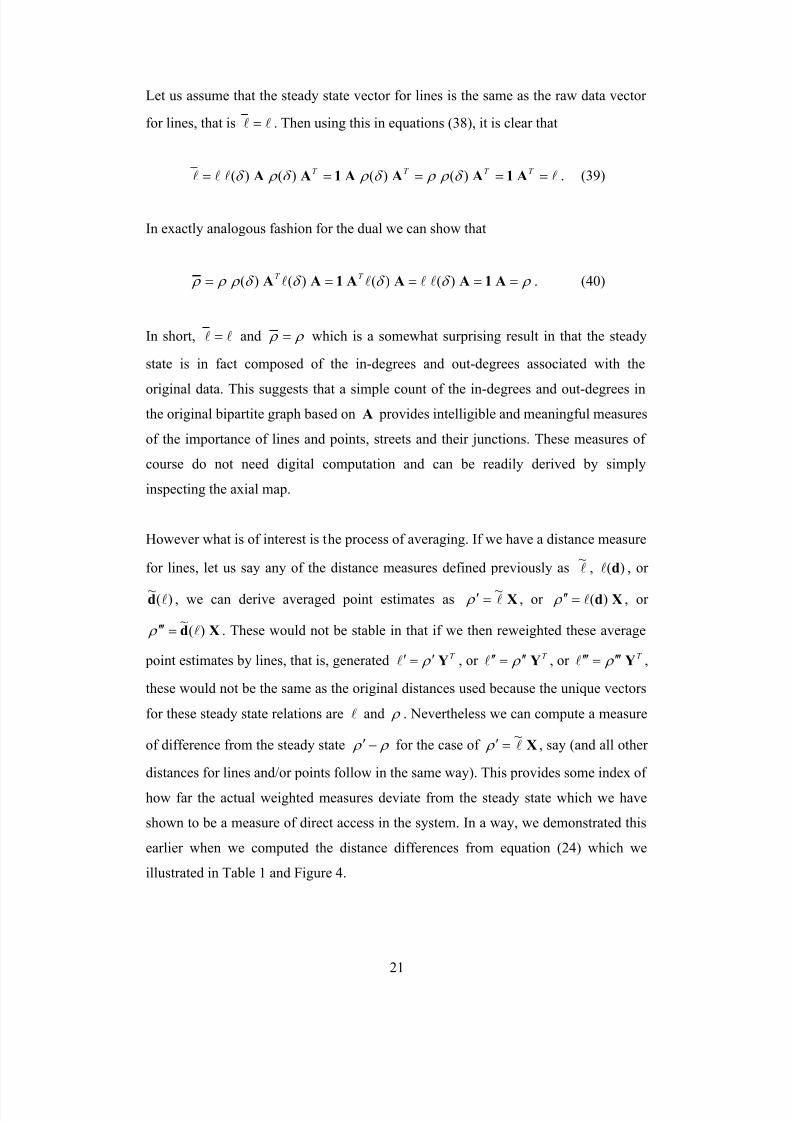
However what is of interest is the process of averaging. If we have a distance measure

for lines, let us say any of the distance measures defined previously as l~

, )(dl , or

)(~ ld , we can derive averaged point estimates as Xl~=′ ρ , or Xd)(l=′′ ρ , or

Xd )(~

l=′′′ ρ . These would not be stable in that if we then reweighted these average

point estimates by lines, that is, generated T Y ρ ′=′l , or T

Y ρ ′′=′′l , or T Y ρ ′′′=′′′l ,

these would not be the same as the original distances used because the unique vectors

for these steady state relations are l and ρ . Nevertheless we can compute a measure

of difference from the steady state ρ ρ −′ for the case of Xl~

=′ ρ , say (and all other

distances for lines and/or points follow in the same way). This provides some index of

how far the actual weighted measures deviate from the steady state which we have

shown to be a measure of direct access in the system. In a way, we demonstrated this

earlier when we computed the distance differences from equation (24) which we

illustrated in Table 1 and Figure 4.



22

6 Demonstrating the New Syntax: Accessibility in the Street Patterns

We have already introduced a little data pertaining to the village of Gassin implying

that the axial map, like most, is sparse in comparison to such sets of relations for non-

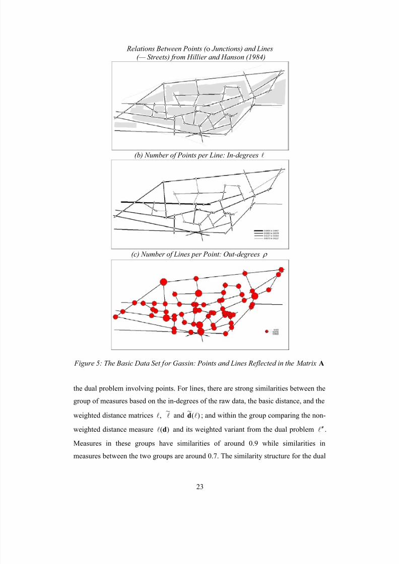
Euclidean systems. The map is shown in Figure 5 along with the in-degree and out-degree distributions ][ il and ][ j ρ which are computed from the raw data matrix A .

The density of links is only 5.1 percent of the total possible for a system in which

every line would be linked to every point and vice versa. The average number of

points per line – junctions per street ni i∑ l – is 3.385 while the average number of

lines per point – streets per junction m j j∑ ρ – is 2.129 which is very close to

planarity. We noted this fact earlier in that 065.1=Ψ meaning that only just above 6

percent of the points are differently configured from an equivalent planar graph. In

fact of the 63 points, only six are associated with more than 2 lines and these involve

only 3 lines each. This is a worrying feature of space syntax in that the systems in

question do not pick up the kind of variation that characterizes other measures of

accessibility such as those in spatial interaction theory. Of even more concern is the

fact that as the relationships between lines – the key emphasis in space syntax – is

based on the number of common points and if most points have only two

such lines, the distribution of topological distances between lines is likely to be rather

narrow, as in fact we note in many applications where the depth or distance in graphs

is seldom more than 6 or 7 step lengths. This means that information pertaining to

distances from numbers of points and lines in common should not be thrown away as

it is in current practice for computing distance, thence integration, in space syntax.

We first examine the similarities between various distance measures for the primal

and dual problem just as we did for the randomized runs which we presented earlier.

We have taken the four distance measures used in Table 1 which are ,l ,~l )(dl and

)(~

ld for the primal, and , ρ ,~ ρ )(d ρ and )(~ ρ d for the dual problems and added the

weighted distance measures ij j ji Y d ∑=′′ )( ρ l and iji i j X d ∑=′′ )(l ρ which appear to

be more discriminating with respect to accessibility than any others. In Table 2(a) we

show these similarity measures for the primal problem involving lines and in 2(b) for



23

Relations Between Points ( ο Junctions) and Lines(— Streets) from Hillier and Hanson (1984)

(b) Number of Points per Line: In-degrees l

(c) Number of Lines per Point: Out-degrees ρ

Figure 5: The Basic Data Set for Gassin: Points and Lines Reflected in the Matrix A

the dual problem involving points. For lines, there are strong similarities between the

group of measures based on the in-degrees of the raw data, the basic distance, and the

weighted distance matrices ,l l~

and )(~

ld ; and within the group comparing the non-

weighted distance measure )(dl and its weighted variant from the dual problem l ′′ .

Measures in these groups have similarities of around 0.9 while similarities in

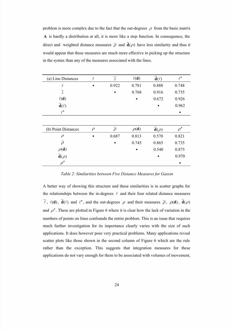
measures between the two groups are around 0.7. The similarity structure for the dual



24

problem is more complex due to the fact that the out-degrees ρ from the basic matrix

A is hardly a distribution at all, it is more like a step function. In consequence, the

direct and weighted distance measures ρ ~ and )(~ ρ d have less similarity and thus it

would appear that these measures are much more effective in picking up the structure

in the syntax than any of the measures associated with the lines.

(a) Line Distances l l~

)(dl )(~

ld l ′′

l • 0.922 0.781 0.888 0.748

l~

• 0.768 0.916 0.735

)(dl • 0.672 0.926

)(~

ld • 0.962

l ′′ •

(b) Point Distances ρ ρ ~ )(d ρ )(~ ρ d ρ ′′

ρ • 0.687 0.813 0.570 0.821

ρ ~ • 0.745 0.865 0.735

)(d ρ • 0.540 0.875

)(~ ρ d • 0.970

ρ ′′ •

Table 2: Similarities between Five Distance Measures for Gassin

A better way of showing this structure and these similarities is in scatter graphs for

the relationships between the in-degrees l and their four related distance measures

l~

, )(dl , )(~

ld and l ′′ , and the out-degrees ρ and their measures ρ ~ , )(d ρ , )(~ ρ d

and ρ ′′ . These are plotted in Figure 6 where it is clear how the lack of variation in the

numbers of points on lines confounds the entire problem. This is an issue that requires

much further investigation for its importance clearly varies with the size of such

applications. It does however pose very practical problems. Many applications reveal

scatter plots like those shown in the second column of Figure 6 which are the rule

rather than the exception. This suggests that integration measures for these

applications do not vary enough for them to be associated with volumes of movement,



25

l~

ρ ~

l ρ

)(dl

)(d ρ

l ρ

)(~

ld

)(~ ρ d

l ρ

l ′′ ρ ′′

l ρ

Figure 6: Scatter Plots of Access Measures from the Data l and ρ against the

Direct and Indirect Distance Measures



26

particularly pedestrian traffic, which they often are. In short, statistical correlations in

many such applications are suspect because there is simply not enough variation in

the basic data; hence our decision to use a measure of similarity, not correlation.

We illustrate these four key distance measures for the primal and dual distributions in

Figure 7, and this provides us with an ability to visually classify the configurational

properties of the syntax. In fact there is nothing in space syntax which actually

provides synoptic measures of morphology in that the only way to examine the

overall pattern is to map the measures, that is, to translate the topological measures

back into Euclidean space and to search for pattern visually. For the lines, we use

conventional space syntax coloring, dividing the range in eight equal classes from

highest (red) to lowest (blue) but we also vary the thickness of the lines to impress the

intensity of the largest values with the thickest lines being red and the thinnest blue.

These four line graphs are quite similar. The central spine through the village and the

increased accessibility in the west is a common feature of each distance while the

lowest values are within the interior where it is hardest to penetrate, and in the south

east of the built-up area. There is some sense in which the northern axis line exerts a

significant influence on accessibility although the fact that this is on the edge of the

village reduces this impact. The strength of each point or junction for each of these

measures is shown using proportional pie charts where it is again clear that the

junctions on the central spine dominate. In both the primal and dual problems, there

seems to be slightly more discrimination with respect to )(~

ld , whereas )(dl and its

derivative l ′′ from the dual problem, emphasize the importance of the northern axis,

as confirmed by an examination of the related point distributions. As one might

expect, there is a clear tie-up between the primal and dual problems in that the

distance measures from one reinforce those from the other.

One of the biggest difficulties in space syntax is in providing a clear interpretation of the map pattern from classifying lines; our brain does not process such linear data

nearly as well as aerial data when we wish to interpret place-related information. One

of the advantages of moving from the primal to the dual, from lines to points, is that

points are place-related and it is easy to generate spheres of influence around them.

Indeed the mapping of accessibility is largely accomplished using surfaces and



27

contours which imply such hinterlands of influence around fixed point locations. This

The Primal Problem: Lines: Streets The Dual Problem: Points: Junctions

Direct Distance l~

Direct Distance ρ ~

Step Distances )(dl Step Distances )(d ρ

Weighted Distances )(~

ld Weighted Distances )(~ ρ d

Line Distance from Weighted Points l ′′ Point Distance from Weighted Lines ρ ′′

Figure 7: Comparison of Distance Measures for the Primal and Dual Problems

is easy enough to accomplish for points but the spheres of influence around lines are

trickier, although not impossible to generate. To illustrate how we might generalize

this problem and provide a means whereby we can compare lines with points and vice

versa in a way which is more consistent than the two representations in Figure 7, we

have used the surface interpolation technique within MapInfo (Professional Version



28

6.5). This enables us to fix a field of influence around each point or line being mapped

and to control the averaging of adjacent points with respect to the usual inverse

distance weighting associated with such interpolation. We have chosen values such

that the influence is as sharp as possible but not too sharp as to destroy the aerial

pattern in the data.

In Figure 8, we show the surfaces associated with the distance measures )(dl and

)(~

ld for the primal problem and it is quite clear that these surfaces are highly

correlated; they reinforce the conclusions already made about the importance of the

central spine and the relative increase in accessibility as one travels west within the

village. As before, )(dl tends to emphasize the northern axis but this is the only

major configurational difference between the two maps. We generate the same two

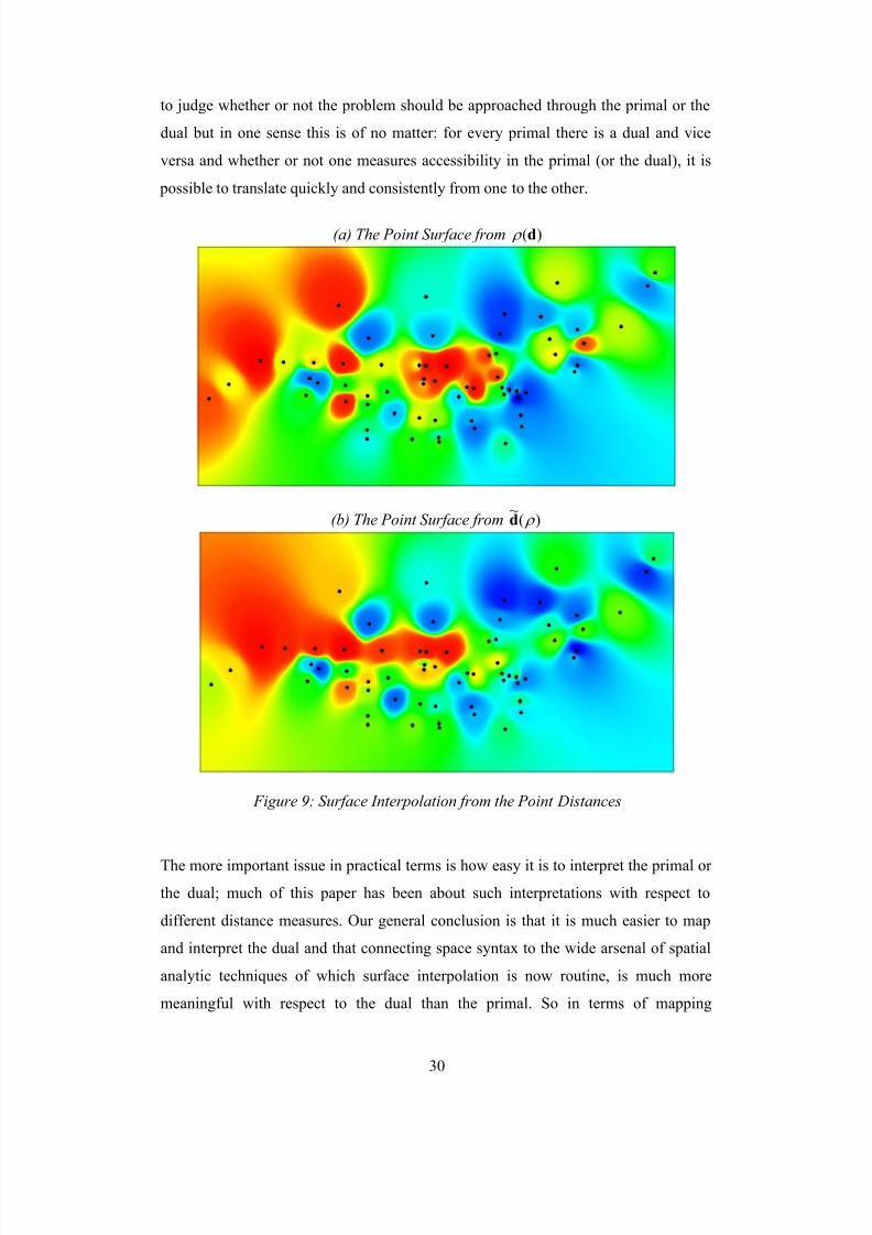
interpolations for points in the dual problems which we show in Figure 9 where we

array the points rather than the lines across the two surfaces. There is a sense in which

these point surfaces reinforce the line surfaces although the influence of each point is

more distinct with slightly less of a ridge line character to these maps. The objection

to such interpolation is that it ignores the influence of buildings and edges although

what it is does do is reinforce the trends in the accessibility surface and gives an

immediate sense of overall variation. It is possible to clip such surfaces to building

features but what we have done here by way of showing how we might move forward

is to simply impose the building extent onto these surfaces, leaving the reader to judge

for him or herself the usefulness of the mapping.

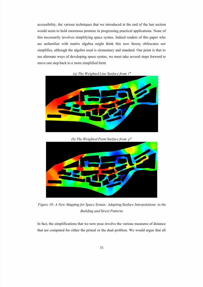
In Figure 10, we have interpolated between the weighted line l ′′ and point ρ ′′

accessibilities and then intersected these surfaces with the buildings and boundary

edges to the village, thus providing a sense of aerial accessibility within the street

system. This is quite an effective technique: what it gives to interpretation that is

missing in the conventional line diagrams in Figure 7 is some sense of trends within

the whole system. There is much more work to do on adapting these visualization

techniques to problems of urban morphology and its syntax but the fact that we are

now able to move from the primal problem to the dual gives some meaning to

interpretations that begin with lines and move to points and back again.



29

(a) The Line Surface from )(dl

(b) The Line Surface from )(~

ld

Figure 8: Surface Interpolation from the Line Distances

7 Next Steps: Simplifying Space Syntax

The essential message of this paper is that the techniques and practice of space syntax

which we consider a special case of accessibility within graphs, is but one way of

looking at the problem of tracing relationships between the relative importance of

streets that make up the urban fabric. The conventional formulation is the primal

problem but as we have shown, there is a dual problem that has equal significance and

consists of measuring the relative importance of the points, junctions, or intersections

that define the location of streets in question. We consider that there are equally good

reasons for considering the dual problem, perhaps more so because it is easier to map

the accessibility of points rather than the accessibility of streets. We leave the reader



30

to judge whether or not the problem should be approached through the primal or the

dual but in one sense this is of no matter: for every primal there is a dual and vice

versa and whether or not one measures accessibility in the primal (or the dual), it is

possible to translate quickly and consistently from one to the other.

(a) The Point Surface from )(d ρ

(b) The Point Surface from )(~ ρ d

Figure 9: Surface Interpolation from the Point Distances

The more important issue in practical terms is how easy it is to interpret the primal or

the dual; much of this paper has been about such interpretations with respect to

different distance measures. Our general conclusion is that it is much easier to map

and interpret the dual and that connecting space syntax to the wide arsenal of spatial

analytic techniques of which surface interpolation is now routine, is much more

meaningful with respect to the dual than the primal. So in terms of mapping



31

accessibility, the various techniques that we introduced at the end of the last section

would seem to hold enormous promise in progressing practical applications. None of

this necessarily involves simplifying space syntax. Indeed readers of this paper who

are unfamiliar with matrix algebra might think this new theory obfuscates not

simplifies, although the algebra used is elementary and standard. Our point is that to

see alternate ways of developing space syntax, we must take several steps forward to

move one step back to a more simplified form.

(a) The Weighted Line Surface from l ′′

(b) The Weighted Point Surface from ρ ′′

Figure 10: A New Mapping for Space Syntax: Adapting Surface Interpolations to the

Building and Street Patterns

In fact, the simplifications that we now pose involve the various measures of distance

that are computed for either the primal or the dual problem. We would argue that all



32

these measures are so highly correlated in problems which in the first instance are

intrinsically embedded in Euclidean space, that their topological structure is quite

simple and that this is reflected in distance measures which take account of all step

lengths in the syntax graph. Thus simply counting in-degrees and out-degrees l and

ρ provides quite good measures of access for lines and points and this of course can

be done manually. Going one step further computing the measures l~

and ρ ~ from the

interaction matrices L and P is easy to do and again provides good direct measures

of access. Although digital computation might be needed for these measures, they

could be produced manually for modest problems and the act of doing so impresses

the importance of what these measures mean in terms of relations between lines

through their common points and points through their common lines. What however

all this suggests is that the starting point for space syntax is not the axial map per se

but the matrix of relations A between lines and points. For each problem, specifying

this matrix formally provides a much more neutral statement of the problem while at

the same time producing an initial examination of its structure.

There are many directions forward that have been implied in this paper. First, the

notion that space syntax is a relation between any two sets of morphological elements,

streets and their junctions in the current kinds of application, is in itself limited. We

need to consider other such elements such as streets and land parcels, different types

of streets, different types of land use, and so on. Second, we can establish chains of

relations such as streets and their intersections, then intersections and their relation to

building plots, then building plots and their relations to land uses, and so on. Such

frameworks need to be formally explored for therein contain the ways in which space

syntax can be linked to other elements of the urban system. Third, there is still more

work to do on distance and accessibility as well as on how we might consistently

embed the physical distance in the street system into space syntax, thus making use of

this information. In a sense, this paper has not been about this issue yet there are promising extensions to the algebra developed here which might show how such

connections can be made.

Fourth, we need to explore how space syntax and related networks relate to small

worlds, the burgeoning statistical theory of graphs, to scaling, to the growth of



33

networks, to neural net conceptions, and so forth which form a cornucopia of potential

research directions already well established. Fifth, we need to sort out how space

syntax relates to standard software. All the computation in this paper is in Quick Basic

and the visualization in MapInfo but it is easy to see how an integrated suite of

programs for calculation and visualization might be fashioned for the desktop. This is

under way in Visual Basic and will be available shortly in the public domain. All of

this constitutes a massive research program for space syntax but only as one corner of

a much wider research program in urban morphology for which new theories of

networks and graphs as well as new techniques of visualization and mapping will

provide the momentum.

8 References

Atkin, R. H. (1974) Mathematical Structure in Human Affairs, Heinemann

Educational Books, London.

Batty, M. (1981) Symmetry and Reversibility in Social Exchange, Journal of

Mathematical Sociology, 9, 1-41.

Batty, M., and Tinkler, K. J. (1979) Symmetric Structure in Spatial and Social

Processes, Environment and Planning B, 6, 3-27.

Coleman, J. (1971) The Mathematics of Collective Action, Heinemann. London.

Dorogovtsev, S. N., and Mendes, J. F. F. (2003) Evolution of Networks: FromBiological Nets to the Internet and WWW, Oxford University Press, Oxford, UK.

Haggett, P., and Chorley, R. J. (1969) Network Analysis in Geography, Edward

Arnold, London.

Hansen, W. G. (1959) How Accessibility Shapes Land Use, Journal of the

American Institute of Planners, 25, 73-76.

Hillier, B. (1996) Space is the Machine: A Configurational Theory of

Architecture, Cambridge University Press, Cambridge, UK.

Hillier, B., and Hanson, J. (1984) The Social Logic of Space, Cambridge University

Press, Cambridge, UK.

Hillier, B., Leaman, A., Stansall, P., and Bedford, M. (1976) Space Syntax,

Environment and Planning B, 3, 147-185.



Hillier, B., Penn, A., Hanson, J., Grajewski, T., and Xu, J. (1993) Natural Movement:

Or Configuration and Attraction in Urban Pedestrian Movement, Environment and

Planning B, 20, 29-66.

Jiang, B., and Claramunt, C. (2000) Integration of Space Syntax into GIS: New

Perspectives for Urban Morphology, Transactions in GIS, 6, 295-307.

Kansky, K. J. (1963) Structure of Transportation Networks: Relationships

Between Network Geometry and Regional Characteristics, Research Paper 84,

Department of Geography, University of Chicago , Chicago, IL.

Kruger, M. (1989) On Node and Axial Maps: Distance Measures and Related Topics,

A paper presented to the European Conference on the Representation and Management

of Urban Change, unpublished.

March, L., and Steadman, J. P. (1971) The Geometry of Environment, RIBA

Publications, London.

Newman, M. E. J. (2003) The Structure and Function of Complex Networks, SIAMReview, 45, 2, 167-256.

Nystuen, J. D., and Dacey, M. F. (1961) A Graph Theory Interpretation of Nodal

Regions, Papers and Proceedings of the Regional Science Association, 7, 29-42.

Steadman, J. P. (1983) Architectural Morphology: Introduction to the Geometry

of Building Plans, Pion Press, London.

Stewart, J. Q. (1947) Suggested Principles of Social Physics, Science, 106, 179-180.

Teklenberg, J. A. F., Timmermans, H. T. P., and van Wagenberg, A. T. (1993) Space

Syntax: Some Standard Integration Measures and Some Simulations, Environment

and Planning B, 20, 347-357.

Watts, D. J. (2003) Six Degrees: The Science of a Connected Age, W.W. Norton and

Company, New York.

Wilson, A. G. (1970) Entropy in Urban and Regional Modelling, Pion Press,

London.

Notes

1 Thanks to Rui Carvalho, Bill Hillier, Alan Penn, and Alasdair Turner who have all

made constructive comments on this paper.

2A more common but different specification of the dual relates to the network of

relations between the interstices formed by the areas bounded by the links in the

original planar graph, see March and Steadman (1971).

paper75 space syntax

Documents