paper no. 2383 - ohio university
TRANSCRIPT

The Influence of Mild Steel Metallurgy on the Initiation of Localized CO2 Corrosion in
Flowing Conditions
Emad Akeer, Bruce Brown, Srdjan Nesic Institute for Corrosion and Multiphase Technology
Department of Chemical and Biomolecular Engineering Ohio University 342 W. State St.
Athens, OH 45701
ABSTRACT The environmental conditions encountered in oil and gas wells can cause severe corrosion to mild steel tubing and pipelines and the microstructure and chemical composition of steel are considered to be important variables that affect the resistance of steel to corrosion. Five different pipeline steels with different chemical composition and microstructure were chosen to investigate the effect of their metallurgy on the properties of iron carbonate and related corrosion phenomena that could lead to localized corrosion. The effect of a high liquid flow rate on a pre-formed iron carbonate corrosion product layer was studied at 80°C, pH 6.6, and 1.5 pCO2. Iron carbonate layer, initially pre-formed on each steel at relatively low wall shear stress (35 Pa), was then exposed to high wall shear stress (535 Pa) for 3 days. For all tested steels, the pre-formed iron carbonate layer reduced the general corrosion rate to less than 0.5 mm/y after 2 days, but the increase in wall shear stress caused partial loss of the protective iron carbonate layer. All steels suffered localized or pitting corrosion, but the penetration rates of pitting found in normalized steels was much lower than that of quenched and tempered steels. Keywords: CO2 corrosion, wall shear stress, iron carbonate, steel microstructure, normalized, quenched and tempered.
©2013 by NACE International.Requests for permission to publish this manuscript in any form, in part or in whole, must be in writing toNACE International, Publications Division, 1440 South Creek Drive, Houston, Texas 77084.The material presented and the views expressed in this paper are solely those of the author(s) and are not necessarily endorsed by the Association.
1
Paper No.
2383

INTRODUCTION
The environmental conditions encountered in oil and gas wells can cause severe corrosion to mild steel tubing and pipelines. Despite this limitation, mild steel is still preferred because it is considered the most cost effective option compared with more expensive alternative materials such as stainless steels (SS), even when including the cost of corrosion inhibition. The ability to protect mild steel pipelines from corrosion is affected by the water chemistry, fluid velocity, CO2 content, and temperature; however, the microstructure and chemical composition of steel are also considered to be important variables 1- 6 that affect the resistance of steel to corrosion.
The use of mild steel in oil and gas pipelines depends on either formation of protective corrosion product layers or use of corrosion inhibitors 5, 6. However, performance of protective corrosion products and corrosion inhibitor are influenced by chemical composition and microstructure of steel 1- 4. Although there are no significant effects of alloying elements and microstructure on corrosion rate in environments where protective layers do not form, when they do, the microstructure and is suspected to cause local areas of accelerated corrosion which vary with metallurgical characteristics. Localized corrosion takes place when small areas of a metal surface selectively experience a higher corrosion rate compared to the rest of the surface. Localized corrosion is known to be very dangerous as it can cause short term failure, over a period of months, of pipelines designed to last for over 20 years. The development of a protective layers on the mild steel surfaces is desirable to limit the corrosion rate, but this layer is highly dependent on surface features and material characteristics. Breakdown of protective layers that form on the mild steel can lead to localized corrosion. Two mechanisms that can cause damage of protective layers are chemical attack and mechanical breakdown. If a large area of a mild steel surface is covered by a protective layer, then failure of a small area on that surface is expected to lead to development of a galvanic cell and accelerate corrosion by an electrochemical mechanism. The chemical and mechanical effect on localized corrosion are dependent on water chemistry and flow parameters; however, it is suspected that chemical composition and microstructure of steel can play a major role in localized corrosion mechanisms in CO2 corrosion.
Many studies have discussed the influence of chemical composition and microstructure of carbon and low alloy steels in CO2 corrosion 1- 6; however, most of these studies did not give a clear explanation relating microstructure and chemical composition of steel to localized corrosion mechanisms in CO2 corrosion.
The goal of this work is to shed light on the influence of pipeline materials on CO2 corrosion of mild steel, with a focus on mechanisms that lead to localized corrosion.
©2013 by NACE International.Requests for permission to publish this manuscript in any form, in part or in whole, must be in writing toNACE International, Publications Division, 1440 South Creek Drive, Houston, Texas 77084.The material presented and the views expressed in this paper are solely those of the author(s) and are not necessarily endorsed by the Association.
2
EXPERIMENTAL PROCEDURE
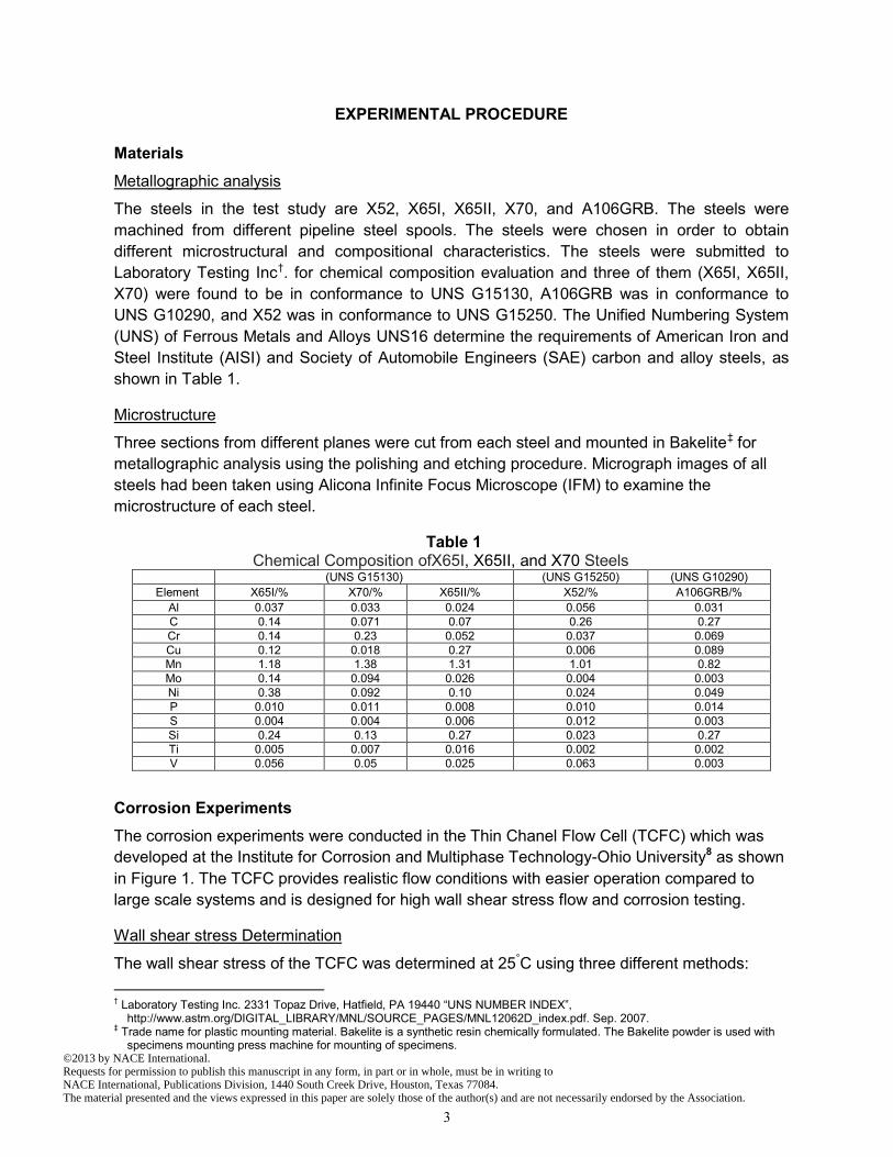
Materials Metallographic analysis
The steels in the test study are X52, X65I, X65II, X70, and A106GRB. The steels were machined from different pipeline steel spools. The steels were chosen in order to obtain different microstructural and compositional characteristics. The steels were submitted to Laboratory Testing Inc†
Table 1
. for chemical composition evaluation and three of them (X65I, X65II, X70) were found to be in conformance to UNS G15130, A106GRB was in conformance to UNS G10290, and X52 was in conformance to UNS G15250. The Unified Numbering System (UNS) of Ferrous Metals and Alloys UNS16 determine the requirements of American Iron and Steel Institute (AISI) and Society of Automobile Engineers (SAE) carbon and alloy steels, as shown in .
Microstructure
Three sections from different planes were cut from each steel and mounted in Bakelite‡
Table 1 Chemical Composition ofX65I, X65II, and X70 Steels
for metallographic analysis using the polishing and etching procedure. Micrograph images of all steels had been taken using Alicona Infinite Focus Microscope (IFM) to examine the microstructure of each steel.
(UNS G15130) (UNS G15250) (UNS G10290) Element X65I/% X70/% X65II/% X52/% A106GRB/%
Al 0.037 0.033 0.024 0.056 0.031 C 0.14 0.071 0.07 0.26 0.27 Cr 0.14 0.23 0.052 0.037 0.069 Cu 0.12 0.018 0.27 0.006 0.089 Mn 1.18 1.38 1.31 1.01 0.82 Mo 0.14 0.094 0.026 0.004 0.003 Ni 0.38 0.092 0.10 0.024 0.049 P 0.010 0.011 0.008 0.010 0.014 S 0.004 0.004 0.006 0.012 0.003 Si 0.24 0.13 0.27 0.023 0.27 Ti 0.005 0.007 0.016 0.002 0.002 V 0.056 0.05 0.025 0.063 0.003
Corrosion Experiments The corrosion experiments were conducted in the Thin Chanel Flow Cell (TCFC) which was developed at the Institute for Corrosion and Multiphase Technology-Ohio University 8 as shown in Figure 1. The TCFC provides realistic flow conditions with easier operation compared to large scale systems and is designed for high wall shear stress flow and corrosion testing.
Wall shear stress Determination
The wall shear stress of the TCFC was determined at 25°C using three different methods: † Laboratory Testing Inc. 2331 Topaz Drive, Hatfield, PA 19440 “UNS NUMBER INDEX”,
http://www.astm.org/DIGITAL_LIBRARY/MNL/SOURCE_PAGES/MNL12062D_index.pdf. Sep. 2007. ‡ Trade name for plastic mounting material. Bakelite is a synthetic resin chemically formulated. The Bakelite powder is used with
specimens mounting press machine for mounting of specimens. ©2013 by NACE International.Requests for permission to publish this manuscript in any form, in part or in whole, must be in writing toNACE International, Publications Division, 1440 South Creek Drive, Houston, Texas 77084.The material presented and the views expressed in this paper are solely those of the author(s) and are not necessarily endorsed by the Association.
3
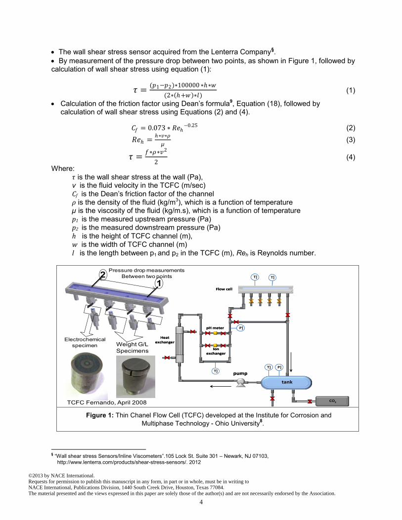
• The wall shear stress sensor acquired from the Lenterra Company§
• By measurement of the pressure drop between two points, as shown in .
Figure 1, followed by calculation of wall shear stress using equation (1):
𝜏𝜏 = (𝑝𝑝1−𝑝𝑝2)∗100000 ∗ℎ∗𝑤𝑤(2∗(ℎ+𝑤𝑤)∗𝑙𝑙)
(1)
• Calculation of the friction factor using Dean’s formula 9, Equation (18), followed by calculation of wall shear stress using Equations (2) and (4).
𝐶𝐶𝑓𝑓 = 0.073 ∗ 𝑅𝑅𝑅𝑅ℎ−0.25 (2) 𝑅𝑅𝑅𝑅ℎ = ℎ∗𝑣𝑣∗𝜌𝜌
µ (3)
𝜏𝜏 = 𝑓𝑓∗𝜌𝜌∗𝑣𝑣2
2 (4)
Where: 𝜏𝜏 is the wall shear stress at the wall (Pa), v is the fluid velocity in the TCFC (m/sec) Cf is the Dean’s friction factor of the channel ρ is the density of the fluid (kg/m3), which is a function of temperature
µ is the viscosity of the fluid (kg/m.s), which is a function of temperature
p1 is the measured upstream pressure (Pa) p2 is the measured downstream pressure (Pa) h is the height of TCFC channel (m), w is the width of TCFC channel (m) l is the length between p1 and p2 in the TCFC (m), Reh is Reynolds number.
Figure 1: Thin Chanel Flow Cell (TCFC) developed at the Institute for Corrosion and
Multiphase Technology - Ohio University 8.
§ “Wall shear stress Sensors/Inline Viscometers”.105 Lock St. Suite 301 – Newark, NJ 07103,
http://www.lenterra.com/products/shear-stress-sensors/. 2012
pump
P]
T] T]
pH meter
Ion exchanger
Flow cell
Heat exchanger
CO2
T] P]T]
tank
pump
P]
T] T]
pH meter
Ion exchanger
Flow cell
Heat exchanger
CO2
T] P]T]
tank
Weight G/L Specimens
Electrochemical specimen
TCFC Fernando, April 2008
1Pressure drop measurements
Between two points2
©2013 by NACE International.Requests for permission to publish this manuscript in any form, in part or in whole, must be in writing toNACE International, Publications Division, 1440 South Creek Drive, Houston, Texas 77084.The material presented and the views expressed in this paper are solely those of the author(s) and are not necessarily endorsed by the Association.
4

Effect of Flow on Formed Iron Carbonate Corrosion Product Layer
Specimen Material - Ten cylindrical specimens (1.25”D, flat weight loss specimens) machined from each steel,
with specific dimensions to fit the corrosion specimen holders that were used in TCFC experiments. In each experiment, one specimen was used for weight loss and the other preserved for surface analysis.
- Linear polarization resistance (LPR) probes were custom designed and built consisting of a concentric ring working electrode (WE) made from the same steel being tested and a center pin reference electrode (RE) made from 306 stainless steel.
Electrolyte An aqueous electrolyte was prepared from deionized water with 1wt. % NaCl. The solution was initially deoxygenated by bubbling with CO2. This procedure assured that the dissolved oxygen levels were kept well below 20 ppb. The pH of the solution was adjusted by adding deoxygenated acid (HCl) or base (NaHCO3) in sufficient quantity to reach the desired pH.
Procedure An iron carbonate layer was generated on each steel by adjusting the concentration of Fe2+ ions, temperature, and pH to the desired levels as shown in Table 2. During the protective layer formation experiments, the volumetric flow from the pump was minimized for a flow velocity through the TCFC of 3.5 m/s (30 Pa wall shear stress) and kept constant for 2 days. These steps ensured surface coverage by the protective iron carbonate layer, as judged by the corrosion rate, which was followed by the LPR measurements. When the protective layer formation was judged complete, the flow rate was increased and the specimens were exposed to high wall shear stress (535 Pa) for 3 days. For the LPR technique, the working electrode was polarized ±10 mV vs. Ecorr. After exposure, the specimens were removed and rinsed immediately in isopropyl alcohol and then dried with cool air and stored in a desiccator, which contains an appropriate flow of nitrogen to facilitate full dessication, until analysis by scanning electron microscopy (SEM) was conducted. After analysis of the corrosion product layer, the weight loss specimens were de-scaled using Clarke solution procedure 10 and corrosion rates were determined from the weight loss. Then visual and infinite focus microscopy (IFM) observations were conducted to qualify the steel surface for any possible localized corrosion.
©2013 by NACE International.Requests for permission to publish this manuscript in any form, in part or in whole, must be in writing toNACE International, Publications Division, 1440 South Creek Drive, Houston, Texas 77084.The material presented and the views expressed in this paper are solely those of the author(s) and are not necessarily endorsed by the Association.
5

Table 2 Test Matrix: TCFC experiments (Localized Corrosion)
Parameters Generate iron carbonate layer Remove iron carbonate layer
Test time 2 days 3 days
Velocity 3.5 m/s 16m/s
wall shear stress 30 Pa 535 Pa
Temperature 80o C
Total Pressure 2.0 bar
CO2Partial pressure 1.5 bar
pH 6.6 (HCl, NaHCO3)
Solution 1.0 wt.% NaCl
Material X52, X65 I, X65 II, X70, A106 GRB
Measurement methods LPR & weight loss
surface morphology IFM, SEM
Initial [Fe++] concentration 18-22 ppm
RESULTS AND DISCUSSION
Metallographic Analysis The micrograph images were examined to determine the microstructure of these steels by comparing the obtained images with a collection of materials micrographs, which have been provided by Micrograph Library, University of Cambridge 11. The microstructures of these steels are described below: X65I & X70: These steels are quenched & tempered (Q & T) and the microstructure consists of tempered martensite, as shown in Figure 2. The microstructures of X65I and X70 are slightly different; the difference could be due to the different carbon content. X65 II: This steel is normalized hot rolled and contains a very low amount of carbon (0.07C) so the resulting microstructure of this steel is ferrite with small amount of pearlite. As shown in Figure 3, there is significant difference in microstructure between planes B, C and plane A. As shown in Figure 3-a, the microstructure of plane A consists of thick light bands of ferrite and thin dark bands of pearlite, which indicate that the steel was probably hot rolled, followed by air cooling to room temperature. Some of the pearlite bands contain yellow gains, which could be related to Cu or Mn. As shown in Figure 3-b, the microstructure of planes B and C consists of light grains of ferrite with some dark pearlite. X52& A106GRB: These steels are normalized and the microstructure consists of large dark grains of pearlite surrounded by large light grains of ferrite, as shown in Figure 4. Clearly different steel microstructures are seen. A summary of chosen steel microstructure and heat treatment is shown in Table 3. There are two steels with large amounts of pearlite, one ferritic steel with only a bit of pearlite and two Q&T steels. This broad variety of microstructures
©2013 by NACE International.Requests for permission to publish this manuscript in any form, in part or in whole, must be in writing toNACE International, Publications Division, 1440 South Creek Drive, Houston, Texas 77084.The material presented and the views expressed in this paper are solely those of the author(s) and are not necessarily endorsed by the Association.
6

may influence the development of iron carbonate precipitation on the surface and the nature of the corrosion product that develops. The goal of this work was to challenge these protective layers to see if they will fail and lead to localized corrosion.
a – X65I (0.14%C) b- X70 (0.071%C)
Figure 2: Q&T Steels (X65I and X70) microstructure consists of tempered martensite.
Plane A Plane B Plane C
a– X65II Plane A b- X65II Plane B
Figure 3: Microstructure of X65II, a normalized hot rolled steel.
a- microstructure consists of thick bright bands of ferrite and thin dark bands of pearlite. b- microstructure consists of small bright ferrite with low amounts of pearlite.
a – X52 b- A106GRB
Figure 4: Normalized Steels (X52 and A106BRB) microstructure consists of large dark pearlite surrounded by large bright ferrite.
Tempered martensite
Quenched & Tempered steel
Tempered martensite
Quenched & Tempered steel
Dark bands of pearliteLight bands of ferrite
Normalized hot rolled steel with low amounts of pearlite.
Yellow grains, could be related to Cu or Mn
PearliteFerrite
Normalized hot rolled steel with small amounts of pearlite.
PearliteFerrite
Normalized steel with large amounts of pearlite.
FerritePearlite
Normalized steel with large amounts of pearlite.
©2013 by NACE International.Requests for permission to publish this manuscript in any form, in part or in whole, must be in writing toNACE International, Publications Division, 1440 South Creek Drive, Houston, Texas 77084.The material presented and the views expressed in this paper are solely those of the author(s) and are not necessarily endorsed by the Association.
7

Table 3
Microstructure and heat treatment of chosen steels.
Steel Carbon content wt% Microstructure Heat treatment
X65I 0.14 Tempered Martensite Quenched & Tempered X70 0.071
X65II 0.07 Ferrite with small amount of pearlite Normalized hot rolled
X52 0.27 Large dark grains of pearlite surrounding by
large light grains of ferrite Normalized A106GR
B 0.26
Corrosion Experiments
Wall shear stress Determination
Figure 5 shows the comparisons between the three methods that have been used to determine the wall shear stress. From the graph it is clear that data collected by direct measurement agree with calculations using Dean’s formula for wall shear stress. The maximum wall shear stress generated in the TCFC was 535 Pascal.
Figure 5: Comparisons of wall shear stress values as determined by different methods.
Iron carbonate Layer Formation and Removal Experiments
Variation of the LPR corrosion rate of all steels with exposure time is shown in Figure 6. No increase in the general corrosion rate, as measured by LPR, was noted beyond 2 days. This indicates that the steels surface was covered by a protective iron carbonate layer. For all steels, after 2 days, the first specimen was removed from the TCFC to document the developed iron carbonate layer and the wall shear stress was then increased to 535 Pa for the
0
100
200
300
400
500
600
700
5 7 9 11 13 15 17
Shea
r St
ress
/ P
a
Velocity / m/secDean's Eq Direct measur_SLED Different Pressure
©2013 by NACE International.Requests for permission to publish this manuscript in any form, in part or in whole, must be in writing toNACE International, Publications Division, 1440 South Creek Drive, Houston, Texas 77084.The material presented and the views expressed in this paper are solely those of the author(s) and are not necessarily endorsed by the Association.
8
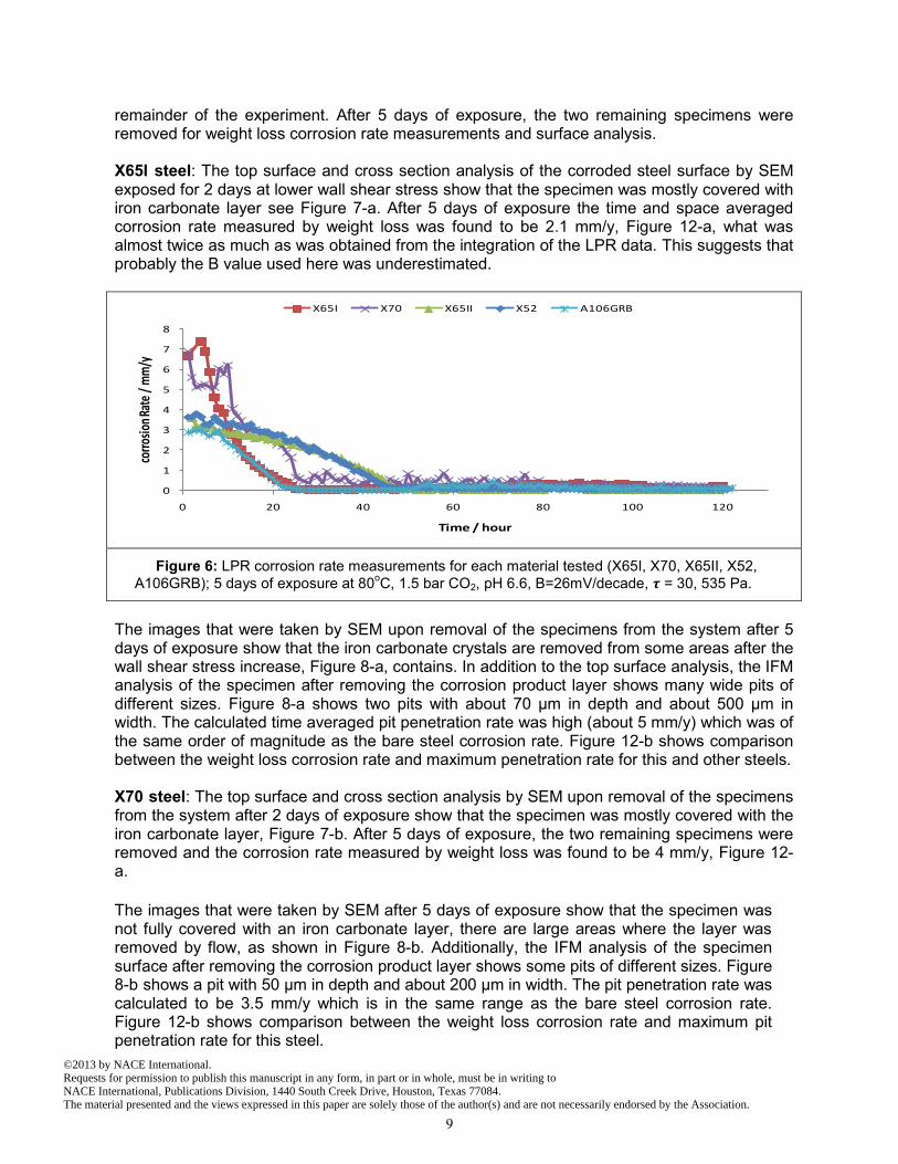
remainder of the experiment. After 5 days of exposure, the two remaining specimens were removed for weight loss corrosion rate measurements and surface analysis. X65I steel: The top surface and cross section analysis of the corroded steel surface by SEM exposed for 2 days at lower wall shear stress show that the specimen was mostly covered with iron carbonate layer see Figure 7-a. After 5 days of exposure the time and space averaged corrosion rate measured by weight loss was found to be 2.1 mm/y, Figure 12-a, what was almost twice as much as was obtained from the integration of the LPR data. This suggests that probably the B value used here was underestimated.
Figure 6: LPR corrosion rate measurements for each material tested (X65I, X70, X65II, X52,
A106GRB); 5 days of exposure at 80οC, 1.5 bar CO2, pH 6.6, B=26mV/decade, 𝝉𝝉 = 30, 535 Pa.
The images that were taken by SEM upon removal of the specimens from the system after 5 days of exposure show that the iron carbonate crystals are removed from some areas after the wall shear stress increase, Figure 8-a, contains. In addition to the top surface analysis, the IFM analysis of the specimen after removing the corrosion product layer shows many wide pits of different sizes. Figure 8-a shows two pits with about 70 µm in depth and about 500 µm in width. The calculated time averaged pit penetration rate was high (about 5 mm/y) which was of the same order of magnitude as the bare steel corrosion rate. Figure 12-b shows comparison between the weight loss corrosion rate and maximum penetration rate for this and other steels. X70 steel: The top surface and cross section analysis by SEM upon removal of the specimens from the system after 2 days of exposure show that the specimen was mostly covered with the iron carbonate layer, Figure 7-b. After 5 days of exposure, the two remaining specimens were removed and the corrosion rate measured by weight loss was found to be 4 mm/y, Figure 12-a.
The images that were taken by SEM after 5 days of exposure show that the specimen was not fully covered with an iron carbonate layer, there are large areas where the layer was removed by flow, as shown in Figure 8-b. Additionally, the IFM analysis of the specimen surface after removing the corrosion product layer shows some pits of different sizes. Figure 8-b shows a pit with 50 µm in depth and about 200 µm in width. The pit penetration rate was calculated to be 3.5 mm/y which is in the same range as the bare steel corrosion rate. Figure 12-b shows comparison between the weight loss corrosion rate and maximum pit penetration rate for this steel.
0
1
2
3
4
5
6
7
8
0 20 40 60 80 100 120
corro
sion R
ate /
mm
/y
Time / hour
X65I X70 X65II X52 A106GRB
©2013 by NACE International.Requests for permission to publish this manuscript in any form, in part or in whole, must be in writing toNACE International, Publications Division, 1440 South Creek Drive, Houston, Texas 77084.The material presented and the views expressed in this paper are solely those of the author(s) and are not necessarily endorsed by the Association.
9

X65I (Q&T Steel) X70 Q&T (Steel)
a – SEM X65I-Top surface analysis b- SEM X70-Cross section analysis
a – SEM X65I-Top surface analysis b- SEM X70-Cross section analysis
Figure 7: SEM,Top Surface and cross section analysis of Q&T steels (X65I, X70), showing iron carbonate layer after 2 days of exposure at 80οC, 1.5 bar CO2, pH 6.6, 𝝉𝝉 = 30 Pa
©2013 by NACE International.Requests for permission to publish this manuscript in any form, in part or in whole, must be in writing toNACE International, Publications Division, 1440 South Creek Drive, Houston, Texas 77084.The material presented and the views expressed in this paper are solely those of the author(s) and are not necessarily endorsed by the Association.
10
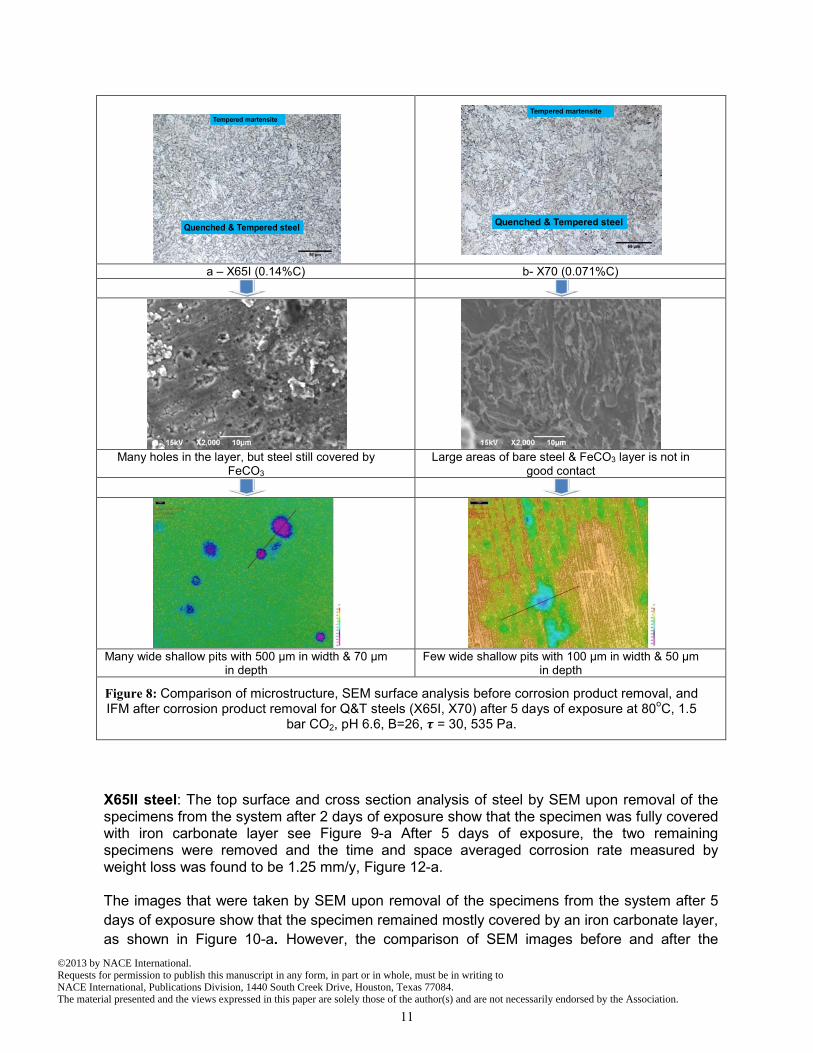
a – X65I (0.14%C) b- X70 (0.071%C)
Many holes in the layer, but steel still covered by
FeCO3 Large areas of bare steel & FeCO3 layer is not in
good contact
Many wide shallow pits with 500 µm in width & 70 µm
in depth Few wide shallow pits with 100 µm in width & 50 µm
in depth
Figure 8: Comparison of microstructure, SEM surface analysis before corrosion product removal, and IFM after corrosion product removal for Q&T steels (X65I, X70) after 5 days of exposure at 80οC, 1.5
bar CO2, pH 6.6, B=26, 𝝉𝝉 = 30, 535 Pa.
X65II steel: The top surface and cross section analysis of steel by SEM upon removal of the specimens from the system after 2 days of exposure show that the specimen was fully covered with iron carbonate layer see Figure 9-a After 5 days of exposure, the two remaining specimens were removed and the time and space averaged corrosion rate measured by weight loss was found to be 1.25 mm/y, Figure 12-a. The images that were taken by SEM upon removal of the specimens from the system after 5 days of exposure show that the specimen remained mostly covered by an iron carbonate layer, as shown in Figure 10-a. However, the comparison of SEM images before and after the
Tempered martensite
Quenched & Tempered steel
Tempered martensite
Quenched & Tempered steel
©2013 by NACE International.Requests for permission to publish this manuscript in any form, in part or in whole, must be in writing toNACE International, Publications Division, 1440 South Creek Drive, Houston, Texas 77084.The material presented and the views expressed in this paper are solely those of the author(s) and are not necessarily endorsed by the Association.
11

increase in wall shear stress shows that the iron carbonate layer after wall shear stress increase, Figure 10-a, contains more voids or holes compared with the specimen before the wall shear stress increase, Figure 9-a. The IFM analysis of the specimen after removing the corrosion product layer from the steel specimen shows several pits with different sizes. Figure 10-a, shows a pit with 80 µm in depth or a 5.8 mm/y pit penetration rate which is of the same order of magnitude as the bare steel corrosion rate. Figure 12-b shows comparison between the corrosion rate and penetration rate of the deepest pit.
X52 steel: The top surface and cross section analysis of steel by SEM upon removal of the specimens from the system after 2 days of exposure show that the specimen was fully covered with iron carbonate layer see Figure 9-b. After 5 days of exposure, the two remaining specimens were removed and the time and space averaged corrosion rate measured by weight loss was found to be 0.75 mm/y, Figure 12-a. The images that were taken by SEM upon removal of the specimens from the system after 5 days of exposure show that the specimen remained mostly covered by an iron carbonate layer, as shown in Figure 10-b. The IFM analysis of the specimen after removing the corrosion product layer from the specimen surface shows some pits of different sizes. Figure 10-b shows a pit with 12 µm in depth and about 400 µm in width. The pit penetration rate was 0.8 mm/y. Figure 12-b, shows comparison between the corrosion rate and penetration rate of the deepest pit.
A106GRB steel: The top surface and cross section analysis by SEM upon removal of the specimens from the system after 2 days of exposure show that the specimen was fully covered with an iron carbonate layer, Figure 9-c. In addition to the top surface and cross-section analysis, the cross-section specimen was etched with 2% Nital and analyzed using SEM to see the relationship between the microstructure of steel and the iron carbonate layer. Figure 11 shows strips or lines of iron carbides extending from the steel substrate into the iron carbonate layer at pearlite grains. This iron carbide structure is thought to enhance the adhesion of the layer in the pearlite areas.
After 5 days of exposure, the two remaining specimens were removed and the time and space averaged corrosion rate measured by weight loss was found to be 0.75 mm/y, Figure 12-a. The images that were taken by SEM upon removal of the specimens from the system after 5 days of exposure show that the specimen appears to be fully covered with an iron carbonate layer, Figure 10-c. Additionally, the IFM analysis of the specimen after de-scaling the specimen shows small pits of different sizes. Figure 10-c shows a pit with 32 µm in depth or 2.3 mm/y pit penetration rate. Figure 12-b, shows comparison between the corrosion rate and penetration rate of the deepest pit.
©2013 by NACE International.Requests for permission to publish this manuscript in any form, in part or in whole, must be in writing toNACE International, Publications Division, 1440 South Creek Drive, Houston, Texas 77084.The material presented and the views expressed in this paper are solely those of the author(s) and are not necessarily endorsed by the Association.
12

X65II (Hot Rolled) X52 (Normalized) A106GRB (Normalized)
a – SEM top surface analysis b – SEM top surface analysis c – SEM top surface analysis
a- SEM Cross section analysis b- SEM Cross section analysis c- SEM Cross section analysis
Figure 9 : SEM, Top Surface and cross section analysis of normalized steels, (X65II, X52, A106GRB, showing iron carbonate layer after 2 days of exposure at 80οC, 1.5 bar CO2, pH 6.6, 𝜏𝜏 = 30 Pa
Lamellar of Carbides present and help to stick the layer to the steel surface
Lamellar of Carbides still present and help to stick the layer to the steel surface
©2013 by NACE International.Requests for permission to publish this manuscript in any form, in part or in whole, must be in writing toNACE International, Publications Division, 1440 South Creek Drive, Houston, Texas 77084.The material presented and the views expressed in this paper are solely those of the author(s) and are not necessarily endorsed by the Association.
13

X65II: Normalized Hot Rolled X52: Normalized A106GRB: Normalized
Some holes but the steel still
covered by FeCO3 layer Completely covered by FeCO3
layer Completely covered by FeCO3
layer
Few pits with 220 µm in width
& 80 µm in depth Few wide shallow pits with 100 µm in width & 12 µm in depth
Many narrow pits with ~30 µm in width & 30 µm in depth
Figure 10: SEM (before corrosion product removal) & IFM (after corrosion product removal) images of normalized steels (X65II, X52, A106GRB) after 5 days of exposure at 80οC, 1.5 bar CO2,
pH 6.6, B=26, 𝝉𝝉 = 30, 535 Pa.
Figure 11: Etched cross section sample of A106GRB steel showing detail of iron carbonate layer
& microstructure after 2 days of exposure at 80οC, 1.5 bar CO2, pH 6.6, 𝝉𝝉 = 30 Pa.
Dark bands of pearliteLight bands of ferrite
Normalized hot rolled steel with low amounts of pearlite.
Yellow grains, could be related to Cu or Mn
PearliteFerrite
Normalized steel with large amounts of pearlite.
FerritePearlite
Normalized steel with large amounts of pearlite.
©2013 by NACE International.Requests for permission to publish this manuscript in any form, in part or in whole, must be in writing toNACE International, Publications Division, 1440 South Creek Drive, Houston, Texas 77084.The material presented and the views expressed in this paper are solely those of the author(s) and are not necessarily endorsed by the Association.
14

a– Corrosion Rate (Weight loss & Integrated LPR) b- Corrosion Rate (WL) & penetration rate
Figure 12:
a- TCFC corrosion rate measured by weight loss (W/L) & integrated LPR after 5 days of exposure at 80οC, 1.5 bar CO2, pH 6.6, 𝜏𝜏 = 30, 535 Pa.
b- Comparison between corrosion rates measured by weight loss (W/L) & penetration rate of the deepest pit on each steel (P/R) LPR after 5 days of exposure at 80οC, 1.5 bar CO2, pH
6.6, 𝜏𝜏 = 30, 535 Pa.
CONCLUSION
- Increasing the wall shear stress caused some locations of the iron carbonate corrosion product layer to fail which may have lead to a high rate of attack (of the same order of magnitude as bare steel corrosion).
- The iron carbonate removal and the pit penetration rates in normalized steels (X52 & A106GRB) were much lower than that pf Q & T steels (X65I & X70).
- The low penetration rates in normalized steels can be related to the homogeneity of microstructure and the pearlite structures which help the iron carbonate layer stray attached to the steel surface.
- The hot rolled steel X65II had the largest pitting penetration rates that could probably be due to inclusions.
ACKNOWLEDGMENT The author would like to thank the Ministry of Higher Education – Libya for financial support, S. Smith (Adjunct Professor for Ohio University, ICMT) and Chevron Corp for technical support. Also thank to all member companies that provide support to the corrosion center.
0
0.5
1
1.5
2
2.5
3
3.5
4
4.5
X65I X70 X65II X52 A106
Corr
osio
n ra
te /
mm
/y
Steels
WL
Integrated LPR
0
1
2
3
4
5
6
7
X65I X70 X65II X52 A106
Corr
osio
n ra
te /
mm
/y
Steels
WL
PR
©2013 by NACE International.Requests for permission to publish this manuscript in any form, in part or in whole, must be in writing toNACE International, Publications Division, 1440 South Creek Drive, Houston, Texas 77084.The material presented and the views expressed in this paper are solely those of the author(s) and are not necessarily endorsed by the Association.
15

REFERENCES 1. D.A. Lopez, T. Perez, and S.N. Simison, “The influence of microstructure and
chemical composition of carbon and low alloy steels in CO2 corrosion. A State-of-the-art appraisal” Elsevier Ltd, Material & Design, vol. 24, pp. 561-575, 2003.
2. A. Dugstad, H. Hemmer, and M. Seiersten, “Effect of Steel Microstructure upon Corrosion Rate and Protective Iron Carbonates Layer Formation, “Corrosion/2000, Houston, TX, NACE, Paper. 24.
3. J. Crolet, N. Thevenot, and S. Nesic, “The role of conductive corrosion products in the protectiveness of corrosion layers,” Corrosion, Vol. 54, no 3, pp.194 –203, 1998.
4. D. Clover, B. Kinsella, B. Pejcic, and R. De Marco, “The influence of microstructure on the corrosion rate of various mild steels ,” Applied Electrochemistry, vol. 35, no 2, pp. 139-149, 2005.
5. T. Berntsen, M. Seiersten, and T. Hemmingsen, “Effect of FeCO3 supersaturation and carbide exposure on the CO2 corrosion rate of mild steel, “Corrosion/2011, Houston, TX, NACE, Paper. 11072.
6. E. Gulbrandsen, R. Nyborg, T, Loland, and K. Nisancioglu, “Effect of steel microstructure and composition on inhibition of CO2 corrosion, “Corrosion/2000, Houston, TX, NACE, Paper. 23.
7. Chevron Corporation, Energy Technology Company, FE - MEE - Corrosion Lab 3901 Briarpark Dr., WP117, Houston, TX 77042 U.S.A.
8. Institute for Corrosion and Multiphase Technology, Ohio University, Research Park, 342 West State Street, Athens, Ohio 45701, Tel: 740-593-0283, Fax: 740-593-9949
9. R. B. Dean. “Reynolds Number Dependence of Skin friction and other Bulk Flow Variables in Two-dimensional Rectangular Duct Flow,” J. Fluids Eng, vol. 100, no 2, pp. 219-242, 1978.
10. ASTM Standard G1, 2003, “Standard Practice for Preparing, Cleaning, and Evaluating Corrosion Test Specimens,” ASTM International, West Conshohocken, PA, 2003, DOI: 10.1520/G0001-03, www.astm.org.
11. Micrograph Library, 2004, University of Cambridge. Available: www.doitpoms.ac.uk/miclib/index.php.
©2013 by NACE International.Requests for permission to publish this manuscript in any form, in part or in whole, must be in writing toNACE International, Publications Division, 1440 South Creek Drive, Houston, Texas 77084.The material presented and the views expressed in this paper are solely those of the author(s) and are not necessarily endorsed by the Association.
16