paper 290517

8/13/2019 Paper 290517

http://slidepdf.com/reader/full/paper-290517 1/27

GCPS 2013 __________________________________________________________________________

Estimate Vibration Risk for Relief and Process Piping

Georges A. Melhem, Ph.D.

ioMosaic Corporation

93 Stiles Road | Salem, NH 03079

[email protected]

© 2013, ioMosaic Corporation; all rights reserved. Do not copy or distribute

without the express written permission of ioMosaic Corporation

Prepared for Presentation at

American Institute of Chemical Engineers

2013 Spring Meeting9th Global Congress on Process Safety

San Antonio, Texas

April 28 – May 1, 2013

UNPUBLISHED

AIChE shall not be responsible for statements or opinions contained

in papers or printed in its publications

8/13/2019 Paper 290517


GCPS 2013 __________________________________________________________________________

Estimate Vibration Risk for Relief and Process Piping

Georges A. Melhem, Ph.D.

ioMosaic Corporation93 Stiles Road | Salem, NH 03079

[email protected]

Keywords: Acoustic induced vibration (AIV), flow induced vibration (FIV), vibration risk,

resonance, singing relief valve.

Abstract

Current API, AIChE/CCPS, and AIChE/DIERS pressure relief and flare systems guidelines andstandards do not formally address vibration risk. They do not offer specific guidance on velocitylimitations other than backpressure calculations and they do not offer guidance on acoustic

induced or flow induced piping vibration fatigue failure. This paper provides a summary of

experience based methods for the estimation of vibration risk in relief and process piping. Inaddition, this paper extends the applicability of the experience based methods to two-phase flow.

1. Introduction

Fatigue failure of relief and/or process piping caused by vibration can develop due to the

conversion of flow mechanical energy to noise. Factors that have led to an increasing incidenceof noise vibration related fatigue failures in piping systems include but are not limited to (a)

increasing flow rates as a result of debottlenecking which contributes to higher flow velocities

with a correspondingly greater level of turbulent energy, (b) frequent use of thin-walled pipingwhich results in higher stress concentrations, particularly at small bore and branch connections,

(c) design of process piping systems on the basis of a static analysis with little attention paid to

vibration induced fatigue, (e) and lack of emphasis of the issue of vibration in piping designcodes. Piping vibration is often considered on an ad-hoc or reactive basis. According to the UK

Health and Safety Executive (HSE), 21 % of all piping failures offshore are caused by

fatigue/vibration. Typical systems at risk include large compressor recycle systems and high

capacity pressure relief depressuring systems. For relief and flare piping, flow inducedturbulence and high frequency acoustic excitations are key concerns.

2. Flow Induced Vibration (FIV)

Fluid flow in pipes generates turbulent energy (pressure fluctuations). Dominant sources ofturbulence are associated with flow discontinuities in the piping systems (e.g., partially closed

valves, short radius, mitered bends, tees or expanders). The level of turbulence intensity is a

function of pipe size, fluid density, viscosity, velocity, and structural support. High noise levels

8/13/2019 Paper 290517


GCPS 2013 __________________________________________________________________________

are generated by high velocity fluid impingement on the pipe wall, turbulent mixing, and if the

flow is choked, shock waves discontinuities downstream of flow restriction. This can lead tohigh frequency excitation / vibration risk.

3. Acoustic Induced Vibration (AIV)

High frequency acoustic energy is often generated by a pressure reducing device such as a relief

valve, control valve, or orifice plate. Acoustic induced piping failure is of a particular concern

for safety related systems (e.g. relief and blowdown/depressuring). The severity of highfrequency acoustic excitation is primarily a function of the pressure upstream and downstream of

the pressure reducing device, pipe diameter, and the fluid volumetric flow. Acoustically induced piping failures are known to occur at non-asymmetric discontinuities in the downstream piping

such as small bore and branch connections and welded supports.

4. Additional Causes of Vibration

Additional causes of piping vibration include mechanical excitation, pulsation, vortex shedding,surge or momentum changes associated with valves, cavitation, and flashing. Mechanical

excitations are often associated with pipes connected with reciprocating compressors, pumps, or

rotating machinery. Such connection machines cause vibration of the pipe and its support

structure. Thermowells are intrusive fittings and are subject to static and dynamic fluid forces.Vortex shedding is the dominant concern as it is capable of forcing the thermowell into flow-

induced resonance and fatigue failure. This is particularly important at high fluid velocities.

5. Relief and Depressuring Systems

Depressuring systems are often subjected to acoustic energy (rapidly fluctuating pressure forces)generated by flow turbulence which is accentuated by flow restricting devices within the flow

path. The magnitude of pressure fluctuations depends on the mass flow rate, speed of sound, and

density. For choked flow, intense noise due to large shock discontinuities and pressurefluctuations is generated. The generated noise is non-periodic due to the randomness of the

pressure fluctuations. Choked flow typically leads to a wide frequency spectrum with peak

values than can exceed 1000 Hz. Vibrations associated with small fittings and branchconnections are of special concern because they introduce discontinuities and stress

concentration points.

In many situations resonance can onset which can lead to magnification of static piping loads upto a factor of 50 times. The presence of discontinuities such as tees and welded pipe supports can

further increase these loads.

6. Noise Generation

A pressure reducing device or relief device controls flow by converting internal energy into

kinetic energy. Some energy is converted to heat through friction (viscous forces) by intense

turbulence and shock formation. Some of the energy is also transferred to the pipe wall as

8/13/2019 Paper 290517


GCPS 2013 __________________________________________________________________________

vibration, and a portion of this is radiated as noise. The primary noise generating mechanism is

the confined jet of fluid formed between the upstream and downstream locations. Flow noise can be modeled as noise of a confined jet. As a result, the noise-generation mechanisms are turbulent

mixing, turbulence boundary interaction, shock, shock/turbulence interaction and flow

separation.

Since the noise is generated downstream of a flow restriction, most of the acoustic energy is

radiated to the downstream piping, which becomes the transmitting medium. As the noise travels

downstream along the inside of the pipe in the fluid it radiates through the pipe wall along itsentire length.

7. How to Calculate Sound Power Level

We can calculate the sound power level in a fundamental way by assigning an efficiency factor

to provide the fraction of flow mechanical energy that is converted to noise:

212

W muη = (1)

2

10 10 1012

110log 10log 120 10log 120

10 2W

W L W muη

−

= = + = +

(2)

where W is the flow mechanical power or energy, W L is the sound power level in dB , and η is

defined as the acoustical efficiency factor. If the flow is choked, then W becomes:

21

2 sonicW muη = (3)

If a value of η can be estimated for single and multi-phase flow, then the sound power level can

be easily calculated not only for pressure reducing devices but also for pipe flow. Attenuationdue to friction and temperature changes can be calculated from pipe flow equations in a more

detailed manner. Computer codes such as SuperChems can then calculate the sound power level

at every axial location for flow piping for single and multi-phase flow. For incompressible flow,the value of flow velocity for an ideal nozzle can be calculated from the mechanical energy

balance:

2

l

u P ρ

= ∆ (4)

Substituting the above equation for u in Equation 1 yields the following Equation for W for

liquid flow through an ideal nozzle:

l

P W mη

ρ

∆= (5)

8/13/2019 Paper 290517


GCPS 2013 __________________________________________________________________________

For liquid flow, a typical value of η is approximately810−.

All gas flow acoustic efficiencies have been reported to approach 1 % of the total flow

mechanical energy for rocketsi. This is illustrated in Figure 1. When the acoustic efficiency is

plotted against the flow mechanical power Figure 1 is obtained. The measured curve indicates

that the acoustic efficiency falls off as the flow mechanical energy gets larger while thecalculated curve

ii indicates increasing acoustic efficiencies.

Figure 1. Acoustic efficiency trends

Two-phase flow sound power level can also be calculated using Equation 1. Recent work bySingh et al.

iii,

iv demonstrated that more attenuation of noise is exhibited by two-phase flow.

Therefore, using the gas acoustic efficiency values will over predict sound power and noiselevels for two-phase flow.

8. Existing Methods and Guidance

Current API, AIChE/CCPS, and AIChE/DIERS pressure relief and flare systems guidelines andstandards do not formally address vibration risk. They do not offer specific guidance on velocity

limitations other than backpressure calculations and they do not offer guidance on acoustic

induced or turbulence induced piping vibration fatigue failure. The Marine TechnologyDirectorate Limited (MTD) has published in 1999 "Guidelines for the Avoidance of Vibration

Induced Fatigue in Process Pipework"v. A second edition of these guidelines were published in

2008 by the Energy Institutevi

. The methods outlined in these guides have been incorporated inthe SuperChems Expert ioVIPER modules. The MTD/Energy Institute guidelines provide

8/13/2019 Paper 290517


GCPS 2013 __________________________________________________________________________

qualitative and quantitative methods for the assessment of piping vibration failure risk and

depending on the calculated risk level they provide generic guidance for the mitigation ofvibration risk.

Many operating companies have established their own internal guidance for evaluating and

minimizing piping vibration risk. Although these criteria vary from company to company, theyall in general include a limit of flow velocity in some form.

A common criteria used in relief systems is to limit the value of flow Mach number to a valueranging from 0.3 to 0.9:

0 3 0 9 sonic

u M

u. ≤ = ≤ . (6)

Another common criteria often encountered is to limit the dynamic pressure component or

kinetic energy of a flow stream to a value of 100,000 Pascals for gas flow:

2 5 21 10 kg m su ρ ≤ × / / (7)

and 50,000 for two-phase flow:

2 5 2110 kg m s

2u ρ ≤ × / / (8)

The 2006 fifth edition of the NORSOK Process Design Standard P-001 limits the flow velocities

for all flare lines to 2 200,000u ρ ≤ 2kg m s/ / for single and multiphase flow. The piping for

flare headers and sub-headers are designed for a maximum Mach number of 0.6 and lines

downstream of pressure relief valves to the first sub-header are designed for a maximum Machnumber of 0.7. For process lines the maximum design velocity for gas pipes is limited to 60

m s/ or0 43

1175u

ρ .≤ whichever is less. The maximum velocity for two-phase lines is limited to

0 5

1183u ρ .≤ or:

2 2 2183 33,489 kg m su ρ ≤ ≤ / / (9)

9. The Method of Carucci and Mueller

Carucci and Mueller have published guidance for the estimation of sound power levels for

control valves and pressure reducing devicesvii, viii.

1 23 6

21 2 110

1

10 log 126 1W

w

P P T L m

P M

.. − = × × × + .

(10)

8/13/2019 Paper 290517


GCPS 2013 __________________________________________________________________________

1 23 6

21 2 110

1

10 log 4 120w

P P T m

P M

.. − = × × × × +

(11)

( )1 2 110 10 10

1

36log 20log 12log 126 1w

P P T m

P M

−= + + + .

(12)

where 1 P is the upstream pressure or source pressure, 2 P is the downstream pressure, 1T is the

source temperature, m is the mass flow rate, and w is the gas molecular weight.

Attenuation of noise due to friction and heat conduction losses is estimated from the following

equation:

0 06W At

i

L L

D,

= . (13)

where L is the pipe length andi

D is the internal pipe diameter. For an L/D of 50 the attenuation

loss is 3 dB. Abrupt changes in flow area (expansion) in the piping can also lead to attenuation.The decrease in sound power level can be estimated from the following equation:

2

1

2 1W Ex

D L

D,

= −

(14)

where 2 1 D D> . A 3 dB reduction is typically applied to the flow leaving a tee in each direction

or entering into a header or a large drum or vessel. The Carucci and Mueller Equation 12 is used by the Energy Institute Guidelines for the assessment of failure likelihood for high frequency

acoustic excitationvi

. Note that the Carucci and Mueller equation cannot be easily applied tocomplex piping systems, multi-phase systems, and relief piping with multiple chokes. Somecompanies also add 6 dB to the sound power level estimate when sonic flow exists at a branch

connection to account for amplified dynamic strain response.

9.1 Analysis of the Carucci and Mueller Data Set Careful analysis of the Carucci and Mueller data set (see Table 1) indicates that the source

pressures were high enough to produce choked (sonic) flow through a flow limiting orifice or

valve upstream of the failure point further downstream, often at a branch or line connection. Thisimportant point was missed by Eisinger who used the downstream (non-choked) flow velocity to

establish his Mach number based failure criterion. We were also able to reproduce Eisinger’sestimates of the original Carucci and Mueller data set based on his published paper.

Carucci and Mueller provided enough data in their original paper to allow the calculation of theupstream flow limiting flow area and choke point conditions (this is possible because they

reported the actual flow rates) as well as the conditions downstream of the flow limiting device

in the discharge piping. Note that the sound power level estimate upstream of the choke pointsshould be based on the pressure difference (or pressure ratio) of the source pressure and the

8/13/2019 Paper 290517


GCPS 2013 __________________________________________________________________________

choke point. The sound pressure level downstream of the choke point (the primary cause of

acoustic induced fatigue failure in downstream piping of the choked point) should be based onthe difference (or pressure ratio) of the choke point and the shock discontinuity pressure

downstream of the choke point. The original equation proposed by Carucci and Mueller used the

pressure difference (or ratio) between the source pressure and the exit pressure downstream of

the choke point. This yields an overestimate of the sound pressure. This overestimate issomewhat tempered by the fact that the pressure difference ratio to the source pressure is raised

to the 3.6 power.

The following information was provided by Carucci and Mueller regarding the five failures and

two high vibrations cases observed in Table 1.

A. Failure occurred during startup. Sonic velocity is achieved at the 6 inch branch

connection of a 24 inch pipe run downstream of the recycle valve. The sound power

level estimate considers the combined acoustic energy generated by the letdown valveand the sonic condition at the branch connection. The upstream pressure at the branch

connection was estimated to be 98.8 psia.

B1/B2. This system consisted of a control valve letting down pressure to a safety valve / flare

header system. The failure occurred after five to ten hours of operation as a crack at a

10 inch branch connection to 28 inch header. Sonic velocity was achieved at both thecontrol valve and the 10 inch branch connection to the 28 inch flare header. As such,

two pertinent data points are established:

1. Acoustic energy within the 10 inch line as generated by valve (not the failure

point), and

2. Combined acoustic energy within the 28 in header as generated by valve andsonic condition at the 10 in branch connection (the failure point).

C. High vibrations, no failures.

D. Failure during startup. Cracks were observed in a 24 inch line downstream of the

compressor recycle valve after twelve hours of operation. The cracks were near the branch connections of a 6 inch line and a 3/4 inch drain valve and at an I-beam support

welded to the pipe at the elbow immediately downstream of the control valve.

E. High vibration, no failures.

F. Failure at severely undercut weld on a 300 mm (12 in.) line made to fasten conduit

support clip. Points of high stress concentration were later eliminated.

G. This system consisted of six, parallel, high pressure steam letdown valves, each with a

downstream, three pass contra-flow attemporator and an in-line silencer. Failure of the

18 inch attemporator shells occurred after four hundred hours of operation.

H. This system included four parallel desuperheaters located downstream of control valves.Several cracks developed in this system after two to three months of operation. Two to

three of the four letdown valves were discharging steam through a 10 inch connection to

8/13/2019 Paper 290517


GCPS 2013 __________________________________________________________________________

a 20 inch header which swaged up to a 30 inch diameter. Longitudinal cracking

occurred at the bottom of the 20 inch header at a transverse guide 0.5 metersdownstream of the fourth 10 inch branch connection. In addition, a 1 inch bypass line

for a block valve downstream of the third letdown valve cracked and the 20 inch header

cracked around a pressure tap downstream of the transverse guide.

Table 1 compares the acoustic efficiencies implied in the Carucci and Mueller method (at the

upstream choke point) vs. acoustic efficiencies established using IEC methods described later on

in this paper. The acoustic efficiencies implied by the Carucci and Mueller method at theupstream choke point ranged from 0.1 to 5 percent while the IEC acoustic efficiency ranged from

0.67 to 1 percent. The Carucci and Mueller method is based on acoustic energy theories

encompassing both jet and choked flow noise as well as test data from work performed by Exxonresearch and engineering. As discussed in later sections, the experience based failure criteria

originally developed by Carucci and Mueller can only be used with sound power levels

calculated by Equation 12.

The implied acoustic efficiency by Equation 12 is proportional to the mass flow rate andinversely proportional to

2u :

1 23 6

2 1

2

1

8 1w

P T m

P M uη

..

= −

(15)

If we consider the case of an ideal gas undergoing isentropic choked (sonic) flow through arestriction orifice, we can establish the following expressions for variables of interest at the

choke point:

1

22

1

T T

γ

=

+

(16)

1

2 1

2

1 P P

γ γ

γ

− =

+ (17)

22

2

w

g

P M

R T ρ = (18)

2

2

g

w

R T u

M

γ = (19)

2 2 om u A ρ = (20)

Substituting the values of mass flow rate m , choked flow velocity 2u , and choke pressure 2 P in

Equation 15, we obtain the following simplified expression for the Carucci and Mueller acousticefficiency after some algebraic manipulations:

8/13/2019 Paper 290517


GCPS 2013 __________________________________________________________________________

Table 1. Vibration risk data set used by Carucci and Mueller and reproduced by Melhem

8/13/2019 Paper 290517


GCPS 2013 __________________________________________________________________________

( )

0 3

1

1

4 7950 2 5882 wo

M P A

T η γ

.

= . − .

(21)

where o A is the effective restriction orifice flow area in 2m , 1 P is the upstream pressure in bara ,

1T is the upstream temperature in Kelvin , and η is the calculated Carucci and Mueller acoustic

efficiency in percent. This expression shows that the Carucci and Mueller acoustic efficiency is

directly proportional to upstream pressure, and the restriction orifice flow area (flow rate). It can be shown that the Carucci and Mueller acoustic efficiency produces unrealistic values for high

pressure systems, large flow area, and/or mixtures with high molecular weights.

If we consider the case of methane discharging through a restriction with an effective flow area

of 0.1 2m , upstream temperature of 373.15 K , and an upstream pressure of 100 bara , the

calculated acoustic efficiency is:

( )0 3

164 7950 1 282 2 5882 100 0 1

373 15η

.

= . × . − . × × .

. (22)

3 559 0 388 100 0 1 13 8%= . × . × × . = . (23)

The same value can also be calculated by calculating m , 2u , 2 P , and η directly from the above

ideal gas flow equations and Equation 15:

12

373 152 2 327 05 K

1 1 282 1

T T

γ

.= = = .

+ . + (24)

1 2821 1 2 82 1

2 1

2 2100 54 9 bara

1 1 282 1 P P

γ γ

γ

.− . −

= = = . + . +

(25)

322

2

54 9 100000 1632 306 kg m

8314 327 03

w

g

P M

R T ρ

. × ×= = = . /

× . (26)

2

2

1 282 8314 327 03466 76 m s

16

g

w

R T u

M

γ . × × .= = = . / (27)

2 2 32 306 466 76 0 1 1507 63 kg som u A ρ = = . × . × . = . / (28)

1 23 6

2 1

2

18 1

w

P T m

P M uη

..

= −

(29)

( )1 2

3 6

2

373 15 1507 638 1 0 549

16 466 76

.

. . . = × − . × ×

. (30)

48 0 0568 43 78 69 2 10−= × . × . × . × (31)

0 1376 or 13 76%= . . (32)

8/13/2019 Paper 290517


GCPS 2013 __________________________________________________________________________

A similar equation to 21 can be derived for the acoustic efficiency downstream of the choke

point:

( ) ( )

3 6 0 3

1

1 1

68 63 4 836 1 1 0397 0 6096 b wo

P M P A

P T η γ γ

. .

= . − . − . + .

(33)

where b P is the superimposed backpressure downstream of the choke point. Applying

Equation 33 to the same example above we calculate an acoustic efficiency of 227 percent at a

backpressure of 1 bara:

( ) ( )3 6 0 3

1 1668 63 4 836 1 282 1 1 0397 0 6096 1 282 100 0 1

100 375η

. .

= . − . × . − . + . × . × × .

62 430 0 9359 0 388 100 0 1= . × . × . × × .

226 70%= . (34)

It is evident from the actual data reported by Carucci and Mueller and from the above theoretical proof that the acoustic efficiency used by Carucci and Mueller in their equation can produceunrealistic values, well in excess of 1 percent.

10. Failure Criteria

Several methods are now available for screening and analyzing the potential failure risk of piping

caused by vibration. These methods include:

• Experience Based - D/t method or D Method

• Experience Based - Mach number method (Not recommended)

• MTD methods

• Detailed structural dynamics methods

The experience based methods center around correlating likelihood of failure based on actualexperience and/or test data. The most widely cited reference is that of Carucci and Mueller (see

vii and viii) for steel pipe.

Figure 2 illustrates the failure criteria developed originally by Carucci and Mueller and latermodified by Eisinger. This failure criteria establishes a design sound power level vs. the ratio of

pipe diameter to thickness. This criteria is fundamentally better than the other criteria based on

pipe diameter only since thicker wall pipes are stronger than thinner wall pipes.

The original work by Carucci and Mueller suggests a limit provided by the following equation

(Figure 2):

2184 6 0 215 184 6 0 215i i

W limit

o i

D D L

D D δ ,

= . − . = . − .−

(35)

8/13/2019 Paper 290517


GCPS 2013 __________________________________________________________________________

where δ is the pipe thickness.

The lower allowable limit developed by Eisinger also shown in Figure 2 is given by the

following equation:

2173 6 0 125 173 6 0 125i i

W limit

o i

D D L

D D δ ,

= . − . = . − .

−

(36)

The NORSOK standard published guidance in 2006 using the same equation forW limit

L,

as

proposed by Eisinger above.

Note that the above limits are based on sound power levels calculated using the source pressure

and the downstream exit pressure. We have recalculated the sound power levels based on the

correct pressure ratios downstream of the choke point. This data is shown in Figures 3, 4, and 5.

Another design limit criterion that was originally proposed by Carucci and Mueller is based on

pipe diameter only for steel pipe. This criterion applies to pipe diameters ranging from 10 inch to36 inch (approximately between 200 mm to 800 mm) and with wall thicknesses ranging from

0.219 in to 0.439 in (approximately 5.5 mm to 10 mm). The design limit is shown in Figure 3 for

the corrected data and can be approximated by:

192 8 9 8 lnW limit L D,

= . − . (37)

where D is the nominal pipe diameter in inches and W L is the sound power limit in dB.

Recent theoretical and experimental work by Chiyoda Engineeringix

indicates that AIV risk will

increase for smaller pipe diameters at the same diameter to thickness ratio. As a result, the

limiting criteria established above should be decreased by 6 dB for an 8 inch pipe, or by 20 log 10

(16/D).

The design limit correlations developed in this paper can be used with computer programs suchas SuperChems Expert which calculates the sound power level at every axial locations for single

and multiphase flow to decide if the steel piping inside diameter to thickness ratio exceed the

allowable limits as shown by Figure 6.

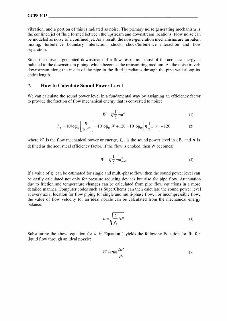
11. Other Methods for Calculating η

The simplest method for calculating η is to assume the same efficiency as an expanded jet (see

Figure 7) and apply it equally to single and multi-phase flow. The efficiency shown in Figure 7 is

the same as what is currently used by API for the estimation of flare noise.

The flow regime types are defined by varying jet shapes in the area upstream and downstream of

the vena contracta. These jets change their shape when certain differential pressure ratios are

exceeded. In regimes II to IV, higher Mach numbers arise downstream of the vena contracta.Yet, M at the vena contracta itself remains unchanged at 1. The IEC method produces equivalent

8/13/2019 Paper 290517


GCPS 2013 __________________________________________________________________________

values of efficiency to the data shown in Figure 7 (as 1 0 L F → . ) as shown in Figure 9. Note that

Figure 9 uses 2 11 x P P = − / as the X axis while Figure 7 uses 1

1 2 1 x P P

−

/ = .

Figure 2. Piping failure limit as originally proposed by Carucci and Mueller and by

Eisinger for steel pipe

The efficiency is related to the flow pressure ratio and the flow regime as well. IEC calculates

the efficiency based on five different flow regimes (see Figure 8) depending on the value of the

downstream pressure, 2 P :

Regime I The flow is sub-sonic. The sound generation has the character of a dipole jet.The highest Mach number is reached at the vena contracta, not exceeding Mach 1 at the

maximum. Downstream of the vena contracta, the jet expands, leading to partial pressure

recovery ( L F factor).

Regime II Sonic and supersonic flows exist together, which means that strongly

turbulent flow and shock cell structure dominate. Pressure recovery drops until the toplimit of regime II is reached.

Regime III The rise in pressure is non-isentropic. The flow is supersonic and shear

turbulence predominates.

Regime IV The shock cells disappear and a Mach disk forms. The dominant mechanism

is the interaction between shock cells and turbulence.

Regime V The acoustical efficiency is constant.

8/13/2019 Paper 290517


GCPS 2013 __________________________________________________________________________

Figure 3. Piping failure correlation developed by Melhem using Carucci Mueller acoustic

efficiency and corrected sound power level estimates for steel pipe. PWL vs. D

Figure 4. Piping failure correlation developed by Melhem using Carucci Mueller acoustic

efficiency and corrected sound power level estimates for steel pipe. PWL vs. D/t

8/13/2019 Paper 290517


GCPS 2013 __________________________________________________________________________

12. Vibration Frequencies

As a fluid moves through piping components there is typically a separation of the fluid from the

constraining wall as the fluid changes flow direction. As a result a vortex is formed and then

swept into the main stream. This vortex shedding occurs at fairly well defined dimensionlessfrequencies. The strength of the vortex varies but does not need to be very strong to cause

damage especially if the shedding frequency couples with the natural frequency of the pipingsystem. The shedding peak frequency for a vortex for subsonic and sonic flows (Regimes I and II

up to a Mach number of 1.4) is given by:

0 2Str p

N u u f

D D= = . (38)

Figure 5. Piping failure correlation developed by Melhem using IEC acoustic efficiency and

corrected sound power level estimates for steel pipe. PWL vs. D/t

where u is the flow velocity in m s/ , D is a characteristic flow dimension (perpendicular to

flow), p f is the peak frequency in Hz and Str N is the Strouhal Number which varies depending

upon the geometry causing the separation of the boundary layer. For a circular cylinder its value

is 0.2 over a wide range of Reynolds numbers. It is usually between 0.1 and 0.3. Vortex shedding

8/13/2019 Paper 290517


GCPS 2013 __________________________________________________________________________

frequencies are generally more than 30 Hz [upper limit for most piping system natural

frequencies].

For flows with Mach numbers larger than 1.4 ( 1 4 M > . , Regimes III to V), the peak frequency

p f is given by:

2

0 4

1 25 1

sonic p

u f D M

.=. −

(39)

For pipe flow, D is equal to the inside flow diameter. For a control valve, D is given by:

0 0046 v l

o

C F D

N = . (40)

Figure 6. Sample piping sound power level calculated by SuperChems Expert v6.4mp vs.

experience based allowable limit for steel pipe

8/13/2019 Paper 290517


GCPS 2013 __________________________________________________________________________

where D is in meters, o N is the number of separate flow passages, vC is the valve flow

coefficient, v

o

C is the channel flow coefficient, and l F is the valve recovery factor. The pressure

recovery factor is defined as:

1 2

1

l

vc

P P F

P P

−=

−

(41)

where 1 2 P P − is the pressure differential across the valve andvc

P is the pressure at the vena

contracta (note that 2 P is larger thanvc

P since the pressure at the exit of the valve recovers):

1 21 2vc

l

P P P P

F

−= − (42)

For liquid flow,vc

P can reach the vapor pressure of the liquid and cause choked flow.

0 96 0 25 vvc f v v

c

P P F P P

P

= ≈ . − .

(43)

Figure 7. Acoustic efficiency of shock noise generated by choked jets, η vs. jet pressure

ratio 1 2 P P / x

where f F is the liquid critical pressure factor, v P is the liquid vapor pressure, and c P is the

liquid critical pressure.

8/13/2019 Paper 290517


GCPS 2013 __________________________________________________________________________

The lowest possible value ofvc

P in a valve flowing liquid would be vacuum or 0. For this

particular limiting case, Equation 41 can be solved for the pressure ratio 1 2 P P / :

1

2

2

1

1d

l

P

P P F = = − (44)

where d P is the damaging pressure ratio. If the valve is operated at a pressure ratio exceeding

d P , the flow will be choked, noisy, and subject to excessive vibration. Table 2 shows typical

valve values for l F and d P .

Within every flowing pipe there will also be a standing wave moving axially back and forth in

the pipe. The frequency of this wave depends on the effective acoustic length of the pipe and thesonic velocity of the fluid in the pipe. The effective acoustic length of the pipe is the distance

between obstructions or acoustic barriers. Examples of obstructions would be valves, pumps, andorifices. An acoustic barrier would be an opening into a larger pipe, a reservoir, the end of a piperun such as a ‘T’ intersection where the branch of interest requires a right angle turn. Piping

components such as expanders or reducers could be an obstruction. An assessment of vibrationrisk should consider both the frequencies with and without the presence of expanders as

obstructions.

The frequency of the standing wave can be calculated as shown below and then compared to the

natural frequencies of valve components and the piping system to determine if there is a potential

for vibration and/or resonance.

Closed End Pipe 4

aci u

L f

∗

=

Open End Pipe 2

aci u

L f

∗=

where 1 2i = , , ... is the wave number, L is the length between acoustic barriers, andac

u is a

characteristic acoustic speed throughout the pipe contents defined as follows:

1

sonicac

dK E

uu

δ

=+

(45)

where sonicu is the speed of sound in the fluid, K is the bulk modulus of elasticity in the fluid, d

is the pipe diameter, δ is the pipe thickness and E is the pipe material of construction modulus

of elasticity.

The above equation is derived from a more general form that depends on the elastic properties of

the pipe:

8/13/2019 Paper 290517


GCPS 2013 __________________________________________________________________________

1

sonicac

K E

uu

ψ =

+ (46)

where ψ is a function of the elastic properties of the pipe. Typical expressions of ψ are shown

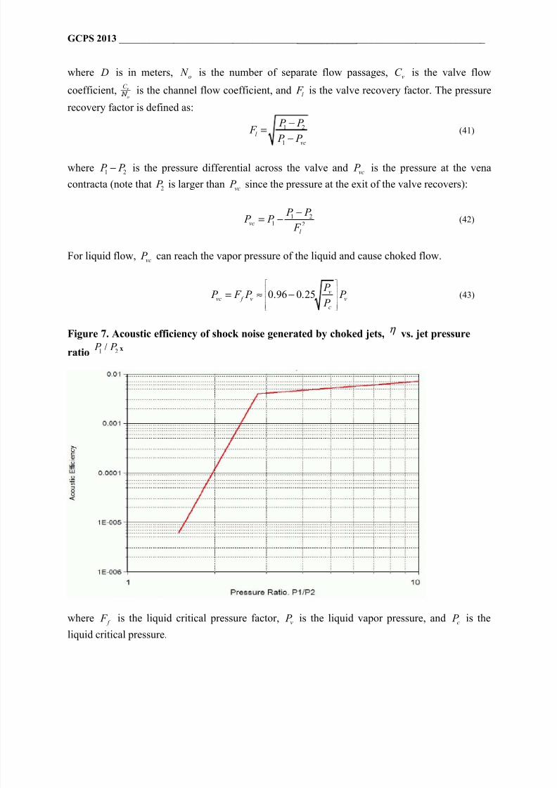
in Table 4. Typical material properties for ψ are shown in Table 3. Note that materials

properties change with temperature as shown in Figure 10.

The speed of sound will change as a function of pressure, temperature, and composition. The

presence of dissolved gas nuclei (such as air or other gases) in compressed liquids cansignificantly reduce the sonic velocity following a pressure drop which leads to the formation of

gas bubbles. Up to 40 % reduction in sonic velocity has been observedxi

.

To control the vibration caused by a standing wave it is necessary to change the magnitude

and/or the frequency of the standing wave or to change the natural frequency of the pipe or

components being excited by the wave. The best approach is to address the magnitude of the

standing wave. The magnitude is related to the fluid turbulent energy that is enforcing the wave.The most dominant source of this turbulence is the kinetic energy generated by the fluid jetexiting the valve trim. Thus a valve change with a trim that reduces this jet energy will eliminate

this wave influence. Trying to change the frequencies is usually not beneficial. There is such a

wide range of frequencies present in the turbulent flow that excitation can continue to establish a

strong wave at the new frequency and continue the piping vibration.

Figure 8. Flow regimes considered for the estimation of acoustical efficiency

8/13/2019 Paper 290517


GCPS 2013 __________________________________________________________________________

Figure 9. IEC flow acoustical efficiency as a function of FL and differential pressure ratio

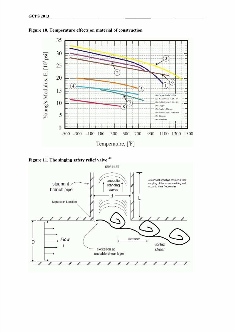
13. The Singing Safety Relief Valve Problem

As a result of increasing steam flow rates, several boiling water reactor (BWR) nuclear power

plants have recently experienced the excitation of acoustic standing waves in closed side branches, e.g., safety relief valves (SRVs), due to vortex shedding generated by steam flow in the

main stream lines. Flow past a valve entrance cavity excites a standing wave, resulting in noiseand vibration

xii. A similar tone is produced when air is blown across the mouth of a glass bottle.

Table 2. Typical valve values for l F and d P

Body Trim FlowDirection

l F 1

2

P

d P P =

Single Seat Globe Cage Open 0.90 5.3Cage Closed 0.80 2.8

V Plug Open 0.90 5.3

V Plug Closed 0.90 5.3

Contoured Open 0.90 5.3Contoured Closed 0.80 2.8

Double Seat Globe V Plug 0.90 5.3

Contoured 0.85 3.6Standard Bore 0.55 1.4

Characterized 0.57 1.5

Angle Cage Open 0.85 3.6Cage Closed 0.80 2.8

8/13/2019 Paper 290517


GCPS 2013 __________________________________________________________________________

Ball 0.8 dia. Orifice 0.55 1.4Butterfly 60

Open 0.68 1.8

Butterfly 90 Open 0.55 1.4

The amplitude of the acoustic pressure waves can be several times higher than the dynamic

pressure present in the system (see Figure 12). The acoustic waves propagate in the steam lines,eventually reaching sensitive components such as steam dryers and turbine stop valves. In

addition, the acoustic waves generated in the side branches may generate vibration problemslocally and may lead to complications such as valve-seat wear. Therefore, the structural

components are subjected to high-cycle fatigue loads, which over time may severely impact

those components’ functionality and safety.

Resonance occurs when the vortex shedding frequency coincides with the acoustic frequency of

the standpipe or the valve components. The natural frequency of the standpipe/valve

combination for a closed end pipe is given by the following equation:

2 1 2 1

4 4 0 425

ac aca

e

u un n f L L L d

− − = = + + .

(47)

where n is the mode number (1 for 1st mode, 2 for 3rd mode, etc.),ac

u is the acoustic speed

through the pipe contents as defined earlier, and e L is an end correction corresponding to

Rayleigh’s upper limit.

The frequency of pressure oscillations (sound) created by vortex shedding, the energy source forthe standing waves, is given by the following equation:

( )0 33 0 25 s str u u f N n

d r d r = ≈ . − .

+ + (48)

Typically peak oscillations occur at a Strouhal Number around 0.4 as shown in Figure 12. Notethat the root mean square pressure amplitude shown in Figure 12 is the ratio of pressure

oscillations divided by dynamic pressure ( 212

u ρ ). RMS begins increasing at a specific onset

Strouhal Number and flow velocity depending on acoustic speed, pipe diameter, and pipe length,

reaches a peak value and then decreases.

There are many similar installations of pressure relief valves in the process industries where the

valves are mounted on large process lines such as overhead lines for distillation columns. Inorder to avoid fatigue failure from resonance caused by the coupling of normal flow vortex

shedding frequency and the acoustic frequency of the standpipe ( s a f f = ), the normal flow

velocity in the main line has to be limited to less than this critical value:

( )1

4

s acmax

st e str

f u d r u d r

N L L N

+< + <

+ (49)

8/13/2019 Paper 290517


GCPS 2013 __________________________________________________________________________

1

4 0 425 0 6

acu d r

L d

+ <

+ . .

As shown in Figure 12 the pressure fluctuations start to increase at a Strouhal number of 0.6 andthen decrease after they reach a peak value around a Strouhal number of 0.4. The same approach

can be applied to the flow through the inlet and/or discharge line of a pressure relief valve:

1

2 0 6

acmax

u Du

L<

. (50)

where L is the acoustic length of the inlet or discharge line. Resonance can also be checked bycomparing an open pipe/contents frequency with the natural frequency of the pressure relief

valve, n f :

1 1

2 2

n sn

n D

K f

m

ω

τ π π = = = (51)

22 D

n

n s

m

K

π τ π

ω = = (52)

where nτ is the undamped natural period in s , and n f is the undamped natural frequency in Hz

where one Hz equals 1 cycle/second, s

K is the spring constant in N m/ , Dm is the mass of the

valve disc and moving parts in kg , and nω is the undamped circular natural frequency in

radians s/ .

14. Conclusions

A general method for the estimation of vibration risk for piping systems for single and

multiphase flow is developed and implemented. An experience based vibration risk failurecriteria is outlined using the work of Carucci and Mueller for gas flow. Because the Carucci and

Mueller sound power level equation can produce unrealistic values of acoustic efficiency, well inexcess of 1 percent for high pressure systems and/or systems with large mechanical flow energy,

the revised experience based failure criteria developed in this paper (see Figure 5) based on the

IEC acoustic efficiency is recommended for multiphase flow.

8/13/2019 Paper 290517


GCPS 2013 __________________________________________________________________________

Figure 10. Temperature effects on material of construction

Figure 11. The singing safety relief valvexiii

8/13/2019 Paper 290517


GCPS 2013 __________________________________________________________________________

Figure 12. Comparison of calculated and measured pressure fluctuations as a function of

Strouhal numberxiv

E is typically referred to as Young’s modulus of elasticity

G is typically referred to as modulus of torsion, 12 1

E Gν +

=

Table 3. Typical data used in the estimation of sonic velocity in pipelines

Material E (GPa) Poisson’s

Ratio ν

1 K κ

=

(GPa)

ρ in kg m3/

Aluminum 69 0.33Brass 78-110 0.36Carbon steel 202 0.303

Cast iron 90-160 0.25Concrete 20-30 0.15

Copper 117 0.36Ductile iron 172 0.30

Fibre cement 24 0.17

High carbon steel 210 0.295Inconel 214 0.29

Mild steel 200-212 0.27

Nickel steel 213 0.31Plastic / Perspex 6.0 0.33

Plastic / Polyethylene 0.8 0.46

Plastic / PVC rigid 2.4-2.75Stainless steel 18-8 201 0.30Water - fresh 2.19 999 at 20 C

Water - sea 2.27 1025 at 15 C

8/13/2019 Paper 290517


GCPS 2013 __________________________________________________________________________

Table 4. Typical expressions for ψ

Pipe condition ψ

Rigid 0

Anchored against longitudinal movement through its length 21d δ ν

−

Anchored against longitudinal movement at the upper end ( )1 25d δ ν . −

Frequent expansion joints present d δ

References

i

W.A. Skipwith. Acoustics technology. Survey SP-5093, NASA National Aeronautics and SpaceAdministration, 1970.

ii C.M. Harris. Handbook of Noise Control . cGraw-Hill Book Co., Inc., 1957.

iii N.R. Miller, G.M. Singh, E. Rodarte and P.S. Hrnjak. Modification of standard aeroacoustic

valve noise model to account for friction and two-phase flow. In ACRC TR-162, pages 1-11.

Mechanical and Industrial Engineering Department, University of Illinois, 2000.

iv N.R. Miller, G.M, Singh, E. Rodarte and P.S. Hrnjak. Prediction of noise generated by

expansion devices throttling refrigerant. In ACRC TR-163, pages 1-13. Mechanical and IndustrialEngineering Department, University of Illinois, 2000.

v MTD. Guidelines for the Avoidance of Vibration Induced Fatigue in Process Pipework . Marine

Technology Directorate Limited (MTD), 1999.

vi Energy Institute. Guidelines for the Avoidance of Vibration Induced Fatigue in Process

Pipework . The Energy Institute, London, England, 2008.

vii V.A. Carucci and R.T. Mueller. Acoustically induced piping vibration in high capacity

pressure reducing systems. In 82-/WAPVP-8, pages 1-13. American Society of MechanicalEngineers, ASME, 1982.

viii

F.L. Eisinger. Designing piping systems against acoustically-induced structural fatigue. In PVP-VOL 328, Flow-Induced Vibration, pages 397-404. American Society of Mechanical

Engineers, ASME, 1982.

ix Hisao Izuchi, Investigation of Pipe Size Effect Against Vibration Risk , Presentation to ioMosaic

Corporation, March 2013, Houston.

x I. Heitner. How to estimate plant noises. Hydrocarbon Processing , 47, 67-74, 1968.

8/13/2019 Paper 290517


GCPS 2013 __________________________________________________________________________

xi V.L. Streeter and E.B. Wylie. Water hammer and surge control. Annual Reviews in Fluid

Mechanics, pages 57-74, 1974.

xii T.M. Mulcahy, S.A. Hambric and V.N. Shah. Flow-induced vibration effects on nuclear power

plant components due to main stream line valve singing. In Ninth NRC/ASME Symposium on

Valves, Pumps, and Inservice Testing, NUREG/CP-0152, volume 6, pages 3B:49-3B:69.

NCR/ASME, 2006.

xiii P. Sekerak. Potential adverse flow effects at nuclear power plants. In 16

th International

Conference on Nuclear Engineering . ICONE16-48900, 2008.

xiv K. Okuyama, F. Inada, Y. Ogawa, R. Morita, S. Takahashi and K. Yoshikawa. Evaluation of

acoustic and flow induced vibration of the BWR main stream lines and dryer. Journal of Nuclear

Science and Technology, 48 (5): 759-776, 2011.

paper 290517

Documents