panel data regression
DESCRIPTION
Panel data regressionTRANSCRIPT

6. Regression with panel data
Key feature of this section:
• Up to now, analysis of data on n distinct entities at a givenpoint of time(cross sectional data)
• Example:
Student-performance data set
Observations on different schooling characteristics in n =420 districts (entities)
• Now, data structure in which each entity is observed at twoor more points of time
−→ Panel data
150

6.1. Structure of panel data sets
Definition 6.1: (Panel data)
Panel data consist of observations on the same n entities at twoor more time periods T . If the data set contains observationson the independent variables X1, X2, . . . , Xk and the dependentvariable Y , then we denote the data by
(X1,it, X2,it, . . . , Xk,it, Yit), i = 1, . . . , n and t = 1, . . . , T,
where the first subscript, i, refers to the entity being observedand the second subscript, t, refers to the date at which it isobserved.
151

Selected observations on cigarette sales, prices, and taxes, by state and year
for U.S. states, 1985–1995
152

Terminology:
• A balanced panel is a panel that has all its observations(focus of this lecture)
• An unbalanced panel is a panel that has some missing datafor at least one time period or for at least one entity
Description of example data set:
• Traffic deaths and alcohol taxes(State Traffic Fatality (STF) data set)
• How effective are various government policies designed todiscourage drunk driving in reducing traffic deaths?
153

Description of example data set: [continued]
• Annual data between 1982–1988 for 48 U.S. states(excluding Alaska and Hawai)
• Important variables:
FATALITYRATE is the number of annual traffic deaths per10000 people in the population in the state
BEERTAX is the ’real’ tax on a case of beer put in 1988U.S. dollars by adjusting for inflation
Various dummy variables indicating state-specific charac-teristics such as legal drinking age and punishment
154

Preliminary analysis:
• In a first step we focus on the two years 1982 and 1988 and,for each year, perform an OLS regression of FATALITYRATE onBEERTAX
• The estimated regression equations (neglecting subscripts)for the 1982 and 1988 data along with the standard errors(in brackets) are given by
FATALITYRATE = 2.01 + 0.15 · BEERTAX (6.1)
(0.15) (0.13)
FATALITYRATE = 1.86 + 0.44 · BEERTAX (6.2)
(0.11) (0.13)
155
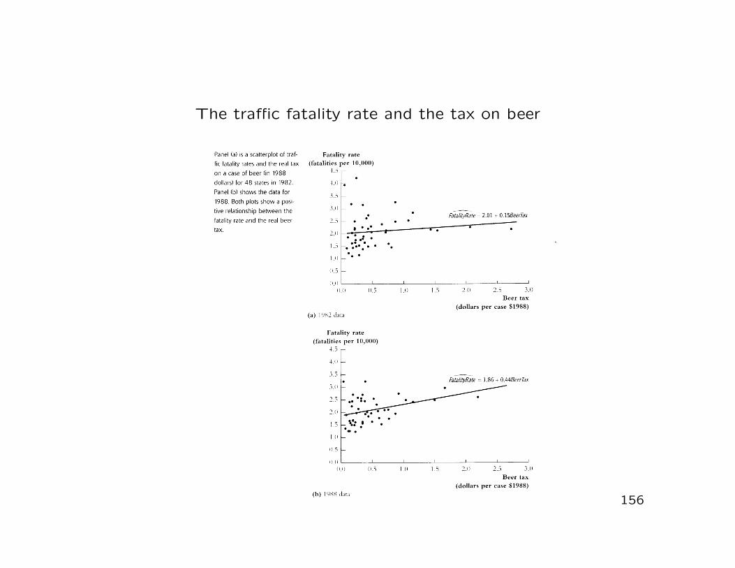
The traffic fatality rate and the tax on beer
156

Preliminary analysis: [continued]
• The OLS estimate β1 for the 1982 data is not significant atthe 10% level(the t-statistic is 1.15 < 1.64)
• The OLS estimate β1 for the 1988 data is significant at the1% level(the t-statistic is 3.43 > 2.58)
• Both OLS estimates are positive what, taken literally, impliesthat higher real beer taxes are associated with more (notfewer) traffic fatalities
−→ Indication of substantial omitted variable bias
157

Preliminary analysis: [continued]
• Some potentially neglected state-specific factors:
Quality of automobiles driven in the state
Quality of state highways
Rural versus urban driving
Density of cars on the road
Cultural acceptance of drinking and driving
158

Problem:
• Some of these variables (such as the cultural acceptance ofdrinking and driving) might be hard or even impossible tomeasure
Possible resort:
• If these factors remain constant over time in a given state,then we make use of the panel data structure to effectivelyhold these factors constant even though we cannot measurethem
−→ OLS regression with fixed effects
159

6.2. Panel data with two time periods: ’before-and-after’ comparisons
Aim of this section:
• Provision of intuition on how we can exploit the panel datastructure to mitigate the omitted-variable-bias problem
Approach:
• We consider a panel with T = 2 time periods
• We focus on changes in the dependent variable
• This ’before-and-after’ comparison holds constant the unob-served factors that differ from one state to the next but donot change over time within the state
160

More explicitly:
• Consider the variable Zi with the following properties:
Zi determines the fatality rate in the ith state
Zi does not change over time(no time-subscript t)
• For example, Zi could represent the local cultural attitudetowards drinking and driving which changes slowly(we consider it to be constant between 1982 and 1988)
• Regression equation:
FATALITYRATEit = β0 + β1 · BEERTAXit + β2 · Zi + uit (6.3)
with i = 1, . . . , n and t = 1,2
161

Now:
• Zi does not change over time
−→ Zi does not produce any change in FATALITYRATE between1982 and 1988
• We eliminate the impact of Zi by analyzing the change inFATALITYRATE between the two periods
Derivation of the change:
• Regression equations for each time period:
FATALITYRATEi1982 = β0 + β1 · BEERTAXi1982 + β2 · Zi + ui1982
FATALITYRATEi1988 = β0 + β1 · BEERTAXi1988 + β2 · Zi + ui1988
162

Derivation of the change: [continued]
• Subtraction of both regression equations:
FATALITYRATEi1988 − FATALITYRATEi1982
= β1 · (BEERTAXi1988 − BEERTAXi1982) + ui1988 − ui1982 (6.4)
Interpretation of Eq. (6.4):
• Zi does not change between 1982 and 1988
−→ Any changes in traffic fatalities over time must have arisenfrom other sources
−→ These changes arechanges in the tax on beerchanges in the error terms(capturing changes in other factors on traffic deaths)
163

More precisely:
• Specifying the regression changes in Eq. (6.4) eliminates theeffect of the unobserved variables Zi that are constant overtime
• Analyzing changes in Y and X has the effect of controllingfor variables that are constant over time thereby eliminatingthis source of omitted variable bias
• Consider the change in the fatality rate between 1982 and1988 against the change in the real beer tax between 1982and 1988 for the 48 U.S. states
164

Changes in fatality rates and beer taxes, 1982–1988
165

Empirical results:
• OLS estimation results:
FATALITYRATEi1988 − FATALITYRATEi1982
= −0.072− 1.04 · (BEERTAXi1988 − BEERTAXi1982) (6.5)
(0.065) (0.36)
• Intercept in Eq. (6.5) allows for the possibility that the meanchange in the fatality rate, in the absence of a change in thereal beer tax, is nonzero
• The negative intercept (−0.072) could reflect improvementsin auto safety from 1982 to 1988 that reduced the averagefatality rate
166

Empirical results: [continued]
• Estimated effect of a change in the real beer tax is negative(as predicted by economic theory)
• OLS slope coefficient of −1.04 is significant at the 1% level(the absolute value of the t statistic is 2.89 > 2.58)
−→ Increase in the real beer tax by 1$ per case reduces thetraffic fatality rate by 1.04 deaths per 10000 people(substantial effect)
Remarks:
• The regression Eq. (6.5) controls for fixed factors such ascultural attitudes towards drinking and driving
• There are other factors influencing traffic safety
167

Remarks: [continued]
• If these factors change over time and are correlated withthe real beer tax, then their omission will produce omittedvariable bias
−→ More careful analysis in Section 6.5
• Transference of the ideas valid for T = 2 to more than 2time periods (T > 2)
−→ Method of fixed effects regression
168

6.3. Fixed effects regression
Now:
• Method for controlling for omitted variables in panel datawhen the omitted variables vary across entities but do notchange over time
• The fixed effects regression model has n different intercepts,one for each entity
• These intercepts can be represented by a set of binary vari-ables
• These binary variables absorp the influences of all omittedvariables that differ from one entity to the next but are con-stant over time
169

More explicitly:
• Consider the regression model (6.3) from Slide 161:
Yit = β0 + β1 ·Xit + β2 · Zi + uit, (6.6)
where Zi is an unobserved variable that varies from one stateto the next but does not change over time(for example, Zi represents cultural attitudes toward drinkingand driving)
• We aim at estimating β1, the effect on Y of X holding con-stant the unobserved state characteristic Z
• We can interpret Eq. (6.6) as having n intercepts, one foreach entity
170

More explicitly: [continued]
• Specifically, define αi ≡ β0+β2 ·Zi, so that Eq. (6.6) becomes
Yit = β1 ·Xit + αi + uit (6.7)
• α1, . . . , αn are treated as state-specific intercepts to be esti-mated
• Population regression line for the ith state: Yit = αi + β1 ·Xit
• The slope coefficient β1 is the same for all states, but theintercept varies from one state to the next
• The intercept αi can be thought of as the ’effect’ of beingin entity i
171

More explicitly: [continued]
• The terms α1, . . . , αn are known as entity fixed effects
• The variation in the entity fixed effects comes from omittedvariables (like Zi in Eq. (6.6)) that vary across entities butnot over time
• Eq. (6.7) is known as the fixed effects regression model
Representation with dummy variables:
• Consider the n− 1 dummy variables
D2,i =
{
1 when i = 20 otherwise
, . . . , Dn,i =
{
1 when i = n0 otherwise
172

Representation with dummy variables: [continued]
• Then, the fixed effects regression model (6.7) can be equiv-alently expressed as
Yit = β0 + β1 ·Xit + γ2 ·D2,i + . . . + γn ·Dn,i + uit, (6.8)
where β0, β1, γ2, . . . , γn are coefficients to be estimated
• Relationships between parameters in Eqs. (6.7) and (6.8):
α1 = β0, α2 = β0 + γ2, . . . , αn = β0 + γn
• The entity-specific intercepts in Eq. (6.7) and the binaryregressors in Eq. (6.8) have the same source, namely theunobserved variable Zi that varies across entities but notover time
173
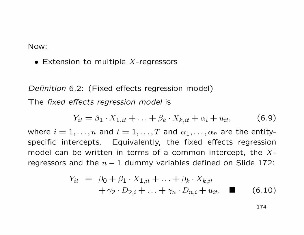
Now:
• Extension to multiple X-regressors
Definition 6.2: (Fixed effects regression model)
The fixed effects regression model is
Yit = β1 ·X1,it + . . . + βk ·Xk,it + αi + uit, (6.9)
where i = 1, . . . , n and t = 1, . . . , T and α1, . . . , αn are the entity-specific intercepts. Equivalently, the fixed effects regressionmodel can be written in terms of a common intercept, the X-regressors and the n− 1 dummy variables defined on Slide 172:
Yit = β0 + β1 ·X1,it + . . . + βk ·Xk,it
+ γ2 ·D2,i + . . . + γn ·Dn,i + uit. (6.10)
174

Estimation and inference:
• In principle, the binary variable specification (6.10) can beestimated via OLS
• However, specificaton (6.10) requires estimation of k+n pa-rameters what becomes problematic if the number of entitiesn is large
−→ Use of special routines for OLS estimation of fixed effectsregressions
• (Two-step) entity-demeaned OLS algorithm
Subtract the entity-specific averages from each variable
Perform OLS regression using the entity-demeaned vari-ables
175

Estimation and inference: [continued]
• Example:
Consider the (single-regressor) fixed effects model (6.7)
Taking (time) averages on both sides of (6.7) yields
Yi = β1 · Xi + αi + ui
with Yi = (1/T )∑T
t=1 Yit and Xi and ui similarly defined
It follows from Eq. (6.7) that
Yit − Yi︸ ︷︷ ︸
≡Yit
= β1 ·Xit + αi + uit − β1 · Xi − αi − ui
= β1 · (Xit − Xi)︸ ︷︷ ︸
≡Xit
+(uit − ui)︸ ︷︷ ︸
≡uit
= β1 · Xit + uit (6.11)
176

Estimation and inference: [continued]
• Example: [continued]
Estimation of β1 in Eq. (6.11) via OLS
• Under certain assumptions stated on Slide 187 (the so-calledfixed effects regression assumptions)
the sampling distribution of the OLS estimator is normalin large samples
the variance and the standard error of the sampling dis-tribution can be estimated from the data
−→ Hypothesis testing (based on t- and F -statistics) and con-struction of confidence intervals in exactly the same wayas in multiple regressions with cross-sectional data
177

Application to traffic deaths:
• OLS estimate of the fixed effects regression based on allT = 7 years of data (observations) is
FATALITYRATE = −0.66 · BEERTAX + StateFixedEffects
(0.29)
• The sign of β1 is negative and the coefficient is significantat the 5% level
• Including state fixed effects avoids omitted variable bias aris-ing from omitted factors that vary across states but are con-stant over time
• What about the effects of omitted factors that evolve overtime but are the same for all states?(for example, overall automobile safety improvements)
−→ Regression with time fixed effects
178

6.4. Regression with time fixed effects
Now:
• We aim at controlling for variables that are constant acrossentities but evolve over time(such as overall safety improvements in new cars)
• To this end, we augment our regression Eq. (6.6) from Slide170 to take the form
Yit = β0 + β1 ·Xit + β2 · Zi + β3 · St + uit, (6.12)
where St is an unobserved variable (representing automobilesafety) that changes over time but is constant across states
• Note that omitting St from the regression may lead to omit-ted variable bias
179
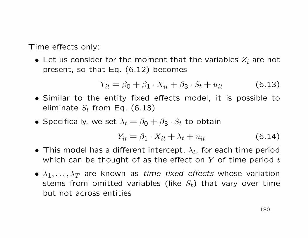
Time effects only:
• Let us consider for the moment that the variables Zi are notpresent, so that Eq. (6.12) becomes
Yit = β0 + β1 ·Xit + β3 · St + uit (6.13)
• Similar to the entity fixed effects model, it is possible toeliminate St from Eq. (6.13)
• Specifically, we set λt = β0 + β3 · St to obtain
Yit = β1 ·Xit + λt + uit (6.14)
• This model has a different intercept, λt, for each time periodwhich can be thought of as the effect on Y of time period t
• λ1, . . . , λT are known as time fixed effects whose variationstems from omitted variables (like St) that vary over timebut not across entities
180

Time effects only: [continued]
• Considering the T − 1 binary variables
B2,t =
{
1 when t = 20 otherwise
, . . . , BT,t =
{
1 when t = T0 otherwise
we can equivalently express model (6.14) as
Yit = β0 + β1 ·Xit + δ2 ·B2,t + . . . + δT ·BT,t + uit, (6.15)
where β0, β1, δ2, . . . , δT are coefficients to be estimated
• Relationships between parameters in Eqs. (6.14) and (6.15):
λ1 = β0, λ2 = β0 + δ2, . . . , λT = β0 + δT
(see Eqs. (6.7) and (6.8) on Slides 171, 173)
181

Now:• Combination of entity and time fixed effects
Definition 6.3: (Entity and time fixed effects regression model)
The fixed effects regression model is
Yit = β1 ·X1,it + . . . + βk ·Xk,it + αi + λt + uit, (6.16)
where α1, . . . , αn are the entity fixed and λ1, . . . , λT time fixedeffects. Equivalently, the entity and time fixed effects regressionmodel can be written in terms of a common intercept, the X-regressors and the n − 1 and T − 1 dummy variables defined onSlides 172, 181:
Yit = β0 + β1 ·X1,it + . . . + βk ·Xk,it+ γ2 ·D2,i + . . . + γn ·Dn,i+ δ2 ·B2,t + . . . + δT ·BT,t + uit. (6.17)
182

Remark:
• The combined entity and time fixed effects regression modeleliminates omitted variables bias arising both from unob-served variables that are constant over time and from vari-ables that are constant across states
Parameter estimation:
• The full model (6.17) can in principle be estimated by OLS
• Most software packages implement a two-step algorithm us-ing entity and time-period demeaned Y and X-variables
183

Application to traffic deaths:
• OLS estimate of the entity and time fixed effects regression:
FATALITYRATE = −0.64 · BEERTAX + SF Effects + TF Effects
(0.36)
• This specification includes
47 state binary variables (state fixed effects, not reported)
6 single-year binary variables (time fixed effects, not re-ported)
the variable BEERTAX
the intercept (not reported)
184

Application to traffic deaths: [continued]
• Time fixed effects have little impact on beer tax coefficient(cf. regression estimation on Slide 178)
• Coefficient is significant at the 10% level(but not at the 5% level; t-statistic is -0.64/0.36 = -1.78)
• Estimation is immune to omitted variable bias from variablesthat are constant either over time or across states
• However, other relevant but omitted variables may vary bothacross states and over time
−→ Specification might still be subject to omitted variable bias
• More careful analysis of the dataset
−→ see class
185

6.5. The fixed effects regression assumptions andstandard errors for fixed effects regression
Aim of this section:
• Formulation of OLS assumptions of the fixed effects regres-sion model so that Theorem 2.4 on Slide 19 holds for theinvolved OLS estimators(especially the asymptotic normal distribution when n is large)
• Some comments on the standard errors for fixed effects re-gressions
186

Definition 6.4: (Fixed effects regression assumptions)
We consider the fixed effects regression model
Yit = β1 ·Xit + αi + uit, i = 1, . . . , n, t = 1, . . . , T.
The following are called the fixed effects regression assumptions:
1. uit has conditional mean zero:
E(uit|Xi1, Xi2, . . . , XiT , αi) = 0.2. (Xi1, Xi2, . . . , XiT , ui1, ui2, . . . , uiT ), i = 1, . . . , n, are i.i.d. draws
from their joint distribution.3. Large outliers are unlikely: Xit and uit have nonzero finite
fourth moments.4. There is no perfect multicollinearity.
For multiple regressors, Xit should be replaced by the full listX1,it, X2,it, . . . , Xk,it.
187

Remarks:
• Definition 6.4 focuses on entity fixed effects regressions ne-glecting time effects
• An extension for including time fixed effects is straightfor-ward
Standard errors for fixed effects regression:
• Autocorrelated errors are a pervasive phenomenon in datawith a time component(see Section 3.1.2. on Slides 48, 49)
• In the case of autocorrelated errors standard errors shouldbe computed using the HAC estimator of the variance
• One type of HAC errors are clustered errors used in thetraffic-fatality dataset
188