NBER WORKING PAPER SERIES

PANEL DATA HEDONICS:ROSEN'S FIRST STAGE AS A "SUFFICIENT STATISTIC"

H. Spencer Banzhaf

Working Paper 21485http://www.nber.org/papers/w21485

NATIONAL BUREAU OF ECONOMIC RESEARCH1050 Massachusetts Avenue

Cambridge, MA 02138August 2015, Revised August 2019

I thank David Albouy, Olivier Beaumais, Kelly Bishop, Jared Carbone, Kerry Smith, Chris Timmins, Reed Walker and Jeffrey Zabel for helpful comments and suggestions on previous drafts. I am especially grateful to Paul Ferraro and Nick Kuminoff for very detailed comments and discussions. I also thank numerous seminar and conference participants. Finally, I thank Kelly Bishop and Chris Timmins for sharing the data used in Section 8. The views expressed herein are those of the author and do not necessarily reflect the views of the National Bureau of Economic Research.

NBER working papers are circulated for discussion and comment purposes. They have not been peer-reviewed or been subject to the review by the NBER Board of Directors that accompanies official NBER publications.

© 2015 by H. Spencer Banzhaf. All rights reserved. Short sections of text, not to exceed two paragraphs, may be quoted without explicit permission provided that full credit, including © notice, is given to the source.

Panel Data Hedonics: Rosen's First Stage as a "Sufficient Statistic" H. Spencer BanzhafNBER Working Paper No. 21485August 2015, Revised August 2019JEL No. D46,D61,H4,Q51,R3

ABSTRACT

Traditional cross-sectional estimates of hedonic price functions can recover marginal willingness to pay for characteristics, but face endogeneity problems for estimating non-marginal welfare measures. I show that when panel data on household demands are available, one can construct a second-order approximation to non-marginal welfare measures using only the first-stage marginal prices. With repeated cross sections of product prices, the measure can be set identified or, under a single-crossing restriction, point identified. Bounds also can be constructed when there are mobility costs. Finally, a variant remains valid when individual preferences shift over time.

H. Spencer BanzhafDepartment of EconomicsAndrew Young School of Policy StudiesGeorgia State UniversityP.O. Box 3992Atlanta, GA 30302and NBERhsbanzhaf@gsu.edu

This paper is a revision of several sections of an earlier paper, "Panel Data Hedonics: Rosen's First Stage and Difference-in-Differences as Sufficient Statistics," which was circulated in August 2015 as Working Paper 21485. A companion paper to this revision, which contains material in the original paper that is not included in this revision, may be found here.

1

Panel Data Hedonics: Rosen's First Stage as a "Sufficient Statistic"

Abstract Traditional cross-sectional estimates of hedonic price functions can recover marginal willingness to pay for characteristics, but face endogeneity problems for estimating non-marginal welfare measures. I show that when panel data on household demands are available, one can construct a second-order approximation to non-marginal welfare measures using only the first-stage marginal prices. With repeated cross sections of product prices, the measure can be set identified or, under a single-crossing restriction, point identified. Bounds also can be constructed when there are mo-bility costs. Finally, a variant remains valid when individual preferences shift over time.

1. Introduction

For decades, the hedonic model has been the starting point for understanding people's values for

differentiated products (see Palmquist 2005 for a review). Its applications include willingness to

pay (WTP) in higher housing prices for local public goods and spatial amenities, compensating

wage differentials for attributes such as job safety, pricing of quality-differentiated consumer prod-

ucts such as computers and cars, and quality-adjustments in national accounting.

Part of the hedonic model's appeal has always been the simple relationship between he-

donic prices and consumer demand: the derivative of a hedonic price function with respect to a

characteristic is equal to a household's marginal WTP for the characteristic. This aspect of the

model is highly appealing because price functions can feasibly be estimated with simple, transpar-

ent research designs, yet they also have a clear welfare interpretation. However, the marginal WTP

potentially observed from only the hedonic price gradient is generally viewed as inadequate infor-

mation for welfare evaluations of large policy shocks. Accordingly, since Rosen (1974), econo-

mists have sought to identify households' willingness-to-pay functions for amenities in a second

stage. But recovering these willingness-to-pay functions from a single cross section has proved to

be a challenge. Because only one point on each individual's demand function is observed (where

marginal WTP is equal to the derivative of the hedonic price function), the only variation in the

data comes from the way different households sort across choice alternatives in equilibrium. The

standard solution is to model heterogeneity in individual demands. Unfortunately, the unobserved

components in demand (e.g. tastes) systematically vary both with levels of amenities and their

marginal prices. This correlation gives rise to a well-known endogeneity problem (Bartik 1987,

2

Epple 1987, Heckman, Matzkin, and Nesheim 2010a, Bishop and Timmins 2019).

Proposed solutions to this problem combine, in one way or another, the economic logic of

sorting along with some structure imposed on heterogeneity in tastes. In the hedonic model,

Ekeland, Heckman, and Nesheim (2004) note that nonlinearities in the equilibrium price function

justify using nonlinear functions of observed demand shifters as instruments for the observed quan-

tities demanded. Heckman, Matzkin, and Nesheim (2005, 2010a) and Bishop and Timmins (2019)

discuss strategies for imposing functional form restrictions that allow one to map quantities of

characteristics into demands. Departing somewhat from the continuous world of the hedonic

model, structural models of discrete choices follow a similar basic strategy (see Kuminoff, Smith,

and Timmins 2013 for a review). In general, because the economics of the models imply a partic-

ular mapping from households' preferences to the way they sort in equilibrium, the logic can be

inverted to recover preferences from observed sorting, conditional on the assumed structure. Typ-

ically, this involves imposing distributional assumptions about unobserved tastes. For example,

they may be assumed to have an extreme value distribution (e.g. Bayer, Ferreira, and McMillan

2007) or a log-normal distribution (e.g. Sieg et al. 2004); similarly, WTP functions may be as-

sumed to have errors following some known distribution (e.g. normal in Bishop and Timmins

2019). Alternatively, one can relax these distributional assumptions but forego point identification

of the underlying parameters (Kuminoff 2012). This literature has provided a tremendous advance

on our ability to model general equilibrium counterfactuals as well as non-marginal welfare ef-

fects. However, these advantages come at the price of imposing additional structure and compli-

cation—thus losing some of the simple reduced-form appeal of the hedonic model.

As Bajari and Benkard (2005), Kuminoff and Pope (2012), and Bishop and Timmins

(2018) have pointed out, the problem becomes considerably easier when individuals are observed

in multiple settings, as then individuals' willingness-to-pay functions can be fitted to two or more

points. To my knowledge, however, the literature has not noticed that when households are ob-

served two or more times, their observed choices, together with knowledge of the first stage he-

donic price functions, are sufficient to estimate welfare measures that are proportional to second-

order approximations to a change in utility for any constant utility function—without explicitly

modeling heterogeneity at all and without imposing any distributional assumptions on unobserved

3

demand parameters.1 With the advent of "big data," such panels are becoming increasingly avail-

able, even in the context of housing markets. For example, in the United States, researchers have

made use of data available under the Home Mortgage Disclosure Act (HMDA) to match house-

holds to the houses they live in over time (e.g. Palmquist 1984 and, more recently, Bayer et al.

2012, and Bishop and Timmins 2018). In principle, such data may be even easier to come by in

other contexts, such as automobile or computer purchases.

In this paper, I show how such data provide an opportunity to reinterpret the hedonic model

in the spirit of calls from Chetty (2009) and Heckman (2010) to seek compromises that combine

the clarity of reduced form econometric models with the ability of structural models to speak to

welfare effects. With multiple time periods, it is possible to combine the logic of the hedonic

model with estimation of only the first stage hedonic price function to identify non-marginal wel-

fare effects under minimal assumptions about demand functions. This is in contrast to the standard

view that knowledge of the hedonic price function alone is insufficient to analyze welfare effects

of large policy shocks with general equilibrium effects. The logic parallels Harberger's (1971)

argument for thinking of consumer surplus in terms of an index number, averaging ex ante and ex

post marginal values. Information from only the first stage can produce a "sufficient statistic" for

welfare measurement.

In particular, I consider monetary measures, constructed from the first-stage hedonic

model, of the change in welfare associated with a change from one hedonic equilibrium to another,

where exogenous amenities, price functions, and even incomes potentially differ. This change is

of interest in at least two contexts. First, we may be interested in comparisons of welfare between

two scenarios, as in cost-of-living indices or comparisons of real income. Banzhaf (2005), Tim-

mins (2006), and Quintero, Epple, and Sieg (2019), among others, consider hedonic approaches to

such questions.2 Second, we may be interested in the general equilibrium effect of specific policy

1 Kuminoff and Pope (2012) suggest using exogenous shifts in the supply of amenities to derive within-market instruments for Rosen's "second stage." Although their suggestion is based on the same basic insight of this paper (that exogenous supply shocks can trace out a demand curve), in contrast I am suggesting that a similar procedure replace the second stage entirely, to identify a sufficient statistic for welfare measure-ment without estimating the deep structural parameters. 2 This application is different from the goal of identifying partial equilibrium welfare measures of (poten-tially) out-of-sample policies. In this sense, this paper follows somewhat in the tradition of the capitaliza-tion literature (Lind 1973, Starrett 1981, Kuminoff and Pope 2014, Banzhaf 2018), in which one looks to changes in the hedonic equilibrium to evaluate in-sample shocks.

4

or information shocks that represent a sudden change in conditions, such as discovery of a cancer

cluster (Davis 2004) or the release of school report cards (Figlio and Lucas 2004). If these involve

exogenous shocks to g or income, we can find the welfare effect of the shocks, even when there

are endogenous changes to hedonic prices and other amenities. This second context is a special

case of the first: if there is one exogenous shock, then the change in conditions can be attributed

to it.

I first show that when one can track households over time, one can construct a second-

order approximation to a Hicksian welfare measure by taking the change in the amenities experi-

enced by the household multiplied by an average of the derivatives of the hedonic price function

over time. The basic model assumes no transactions costs and constant demand functionals (of

hedonic price functions) over time.

I next show that even if one cannot track households over time, one can bound the approx-

imation by "searching" over all possible ways that households sort, using a simple linear program

that respectively minimizes or maximizes the welfare measure. Alternatively, one can impose

additional structure (in particular, a single crossing property) to impute how households sort. As

I discuss in the paper, even if this property is not taken as literally true, as long as sorting patterns

are correlated over time, errors from the assumption largely cancel out, so it makes for a reasonable

approximation.

Finally, I relax the assumptions of no transactions costs and constant demands. In the case

of no transactions costs, I again derive bounds on the welfare measure of interest in the case where

households are myopic. If they are forward-looking, the recent results of Bishop and Murphy

(2019) apply. In the case of constant demands, I show how the approach of the paper can be re-

interpreted as evaluating welfare from a single time period's perspective, a paradigm suggested by

Fisher and Shell (1972) and Pollak (1989).

Additionally, I demonstrate these results using both simulations of hedonic equilibria and

an empirical application. The results of the simulations are consistent with the predicted relation-

ships to true values. The sufficient statistic approach is a compromise between two Hicksian wel-

fare measures, compensating variation (CV) and equivalent variation (EV). I also find that, when

we relax some of the required assumptions, the bounds on welfare hold. The empirical application

illustrates how hedonic data, such as those in a recent application to reductions in violent crime

5

(Bishop and Timmins 2019), can easily be used to compute welfare estimates. The results are

similar to estimates from the more structural model of Rosen (1974).

To fix ideas, I specifically discuss the example of housing markets with spatially varying

amenities and I primarily discuss connections to that literature. However, the implications of this

paper are not limited to that setting and apply equally to labor markets or to other contexts with

differentiated commodities.

2. Model Basics

Consider a closed city (or region) with a constant set of households.3 Let ℋ denote the set of

houses with typical element h and let ℐ denote the set of households with typical element i. Equi-

librium at each point in time consists of a bijective mapping of households to houses (all house-

holds occupy a house and all houses are occupied by a household). For expositional purposes,

residents and landlords can be thought of as two separate groups, but there is nothing requiring

this assumption.

Houses are differentiated by price p, an exogenous amenity g, and a vector of continuous

housing characteristics x with characteristics indexed by r={1,…,R} (lot size, dwelling size, and

so forth). (The variable g may be thought of as an index of public goods, or alternatively other

public goods of secondary interest may be thought to be embedded in x.) Notationally, it will

sometimes be more convenient to work with a more parsimonious notation with the vector z' = [g,

x'] and with the elements of z indexed by j.

At any point in time t, households differ by their income y and by their current-period

preferences, which can be represented by a twice differentiable quasi-concave conditional indirect

utility function 𝑣𝑣𝑖𝑖𝑡𝑡(𝑦𝑦𝑖𝑖𝑡𝑡-ph, gh, xh), with 𝜕𝜕𝑣𝑣𝑖𝑖𝑡𝑡/𝜕𝜕𝑦𝑦𝑖𝑖𝑡𝑡 > 0 and 𝜕𝜕𝑣𝑣𝑖𝑖𝑡𝑡/𝜕𝜕g ≠ 0 everywhere ∀ i. Note that

−𝜕𝜕𝑣𝑣𝑖𝑖𝑡𝑡/𝜕𝜕𝜕𝜕 = 𝜕𝜕𝑣𝑣𝑖𝑖𝑡𝑡/𝜕𝜕𝑦𝑦𝑖𝑖𝑡𝑡 ≡ 𝜆𝜆𝑖𝑖𝑡𝑡, the marginal utility of money.

On the supply side of the market, the profit function for house h is πh = ph - ch(xh), where

the cost function ch( ) is twice differentiable. For convenience, ch( ) is constant over time, although

this assumption could be relaxed.

3 The area modeled does not literally need to be one city (or housing market). Nor need it coincide with the area affected by the policy of interest. However, as always, economists modeling demand must make judgments about the set of relevant substitutes.

6

Consider two moments in time, with t=0 in the initial situation and t=1 in a later situation.

Let Ft( ) be the distribution function of g at time t. Prices of houses are determined by the amenities

and the equilibrium price function: 𝜕𝜕ℎ𝑡𝑡=𝜕𝜕𝑡𝑡(gℎ𝑡𝑡 , 𝐱𝐱ℎ𝑡𝑡 ). The time superscript on the hedonic price

function indicates that equilibrium hedonic prices may shift over time, because of changes in g, in

income, or other aspects of the economic environment. In the initial situation, the household max-

imizes utility over a continuous choice set defined by the continuously differentiable hedonic func-

tion p0=p0(g0, x0). There is then an exogenous shock to the distribution of g available in the city,

and/or to incomes. Consequently, the equilibrium price function adjusts to p1=p1(g1, x1), with the

set of other available characteristics x possibly changing endogenously. It is this change in the

hedonic environment that will be evaluated.

Initially, I make the standard hedonic assumption that households are in a static equilibrium

at both points in time, either because they choose a new product regularly (as would be fitting for

applications to consumer products) or because they can costlessly re-optimize.4 Maximizing util-

ity at time t, the household satisfies the first-order condition:

(1) 𝜕𝜕𝜕𝜕𝑡𝑡

𝜕𝜕𝑧𝑧𝑗𝑗 = −

𝜕𝜕𝑣𝑣𝑖𝑖𝑡𝑡 𝜕𝜕𝑧𝑧𝑗𝑗�𝜕𝜕𝑣𝑣𝑖𝑖𝑡𝑡 𝜕𝜕𝜕𝜕⁄ =

𝜕𝜕𝑣𝑣𝑖𝑖𝑡𝑡 𝜕𝜕𝑧𝑧𝑗𝑗�𝜆𝜆𝑖𝑖𝑡𝑡

.

Equation (1) represents the standard tangency condition, in which the derivative of the hedonic

function with respect to an amenity is equal to marginal WTP for the amenity at the optimal point.

Similarly, the landlord's first-order condition for profit maximization is

(2) 𝜕𝜕𝑐𝑐ℎ𝜕𝜕𝑥𝑥𝑟𝑟

= 𝜕𝜕𝜕𝜕𝑡𝑡

𝜕𝜕𝑥𝑥𝑟𝑟.

That is, the endogenous amenities x are supplied according to similar tangency condition, with

marginal cost of supply equal to the marginal revenue.

4 This assumption continues to underlie the vast majority of work on hedonic markets (e.g. Ekeland, Heck-man, and Nesheim 2004, Bajari and Benkard 2005, Heckman, Matzkin, and Nesheim 2010, Bishop and Timmins 2018) as well as structural sorting models of locational choice (e.g. Sieg et al. 2004 Bayer, Fer-reira, and McMillan 2007, Kuminoff 2012). However, recent work is beginning to consider dynamic opti-mization in the context of transaction costs, which may be substantial in applications to housing (Kennan and Walker 2011, Bishop 2012, Bayer et al. 2016, Bishop and Murphy 2019). The labor literature has a longer tradition of considering such dynamic optimization (e.g. Keane and Wolpin 1997).

7

The basic problem is to make inferences about non-marginal welfare effects from these

primitive conditions.

3. Non-Marginal Values when Demands are Constant and a Panel of Households Is Availa-ble: The Hedonic Harberger Triangle

As a starting point, consider the arguably restrictive case covered by the following three assump-

tions.

ASSUMPTION A1 (Panel of Households). Panel data on household choices are available, so that p and 𝜕𝜕𝜕𝜕𝑡𝑡 𝜕𝜕𝑧𝑧𝑗𝑗� can be evaluated for each household at each point in time at their choice of z.

ASSUMPTION A2 (No transactions Costs). There are no transactions costs, so the household always satisfies the first-order condition given by Equation (1).

ASSUMPTION A3 (Constant Preferences). Households' preferences are constant over the time pe-riod considered: 𝑣𝑣𝑖𝑖𝑡𝑡(𝑦𝑦𝑖𝑖𝑡𝑡-ph, gh, xh) = 𝑣𝑣𝑖𝑖(𝑦𝑦𝑖𝑖𝑡𝑡-ph, gh, xh) ∀ t, so that the optimal vector x and g are unchanging functionals of income and the hedonic price function.

In this subsection, I show that, under Assumptions A1-A3, a second-order approximation

of the general equilibrium welfare effects of a change in conditions can be constructed using only

estimated marginal prices from the first stage hedonic price regression and aggregate changes in

income. The assumptions essentially guarantee that observed shifts in the hedonic price function

trace out the marginal value function (A2 and A3), and that points on the function are observed

(A1). In subsequent sections, Assumptions A1-A3 will be relaxed in turn.

Following Harberger (1971), consider a second order approximation to a change in utility

for an individual in the hedonic model given Assumption A2:

(3)

∆𝑣𝑣𝑖𝑖 ≈ 𝜕𝜕𝑣𝑣𝑖𝑖𝜕𝜕𝑦𝑦

(∆𝑦𝑦𝑖𝑖 − ∆𝜕𝜕𝑖𝑖) + �𝜕𝜕𝑣𝑣𝑖𝑖𝜕𝜕𝑧𝑧𝑗𝑗

∆𝑧𝑧𝑗𝑗,𝑖𝑖𝑗𝑗

+12𝜕𝜕2𝑣𝑣𝑖𝑖𝜕𝜕𝑦𝑦2

(∆𝑦𝑦𝑖𝑖 − ∆𝜕𝜕𝑖𝑖)2

+ �𝜕𝜕2𝑣𝑣𝑖𝑖𝜕𝜕𝑦𝑦𝜕𝜕𝑧𝑧𝑗𝑗

(∆𝑦𝑦𝑖𝑖 − ∆𝜕𝜕𝑖𝑖)∆𝑧𝑧𝑗𝑗,𝑖𝑖𝑗𝑗

+12� �

𝜕𝜕2𝑣𝑣𝑖𝑖𝜕𝜕𝑧𝑧𝑗𝑗𝜕𝜕𝑧𝑧𝑗𝑗′𝑗𝑗𝑗𝑗′

∆𝑧𝑧𝑗𝑗,𝑖𝑖∆𝑧𝑧𝑗𝑗′,𝑖𝑖,

where ∆𝜕𝜕𝑖𝑖 = 𝜕𝜕1(g𝑖𝑖1, 𝐱𝐱𝑖𝑖1) − 𝜕𝜕0(g𝑖𝑖0, 𝐱𝐱𝑖𝑖0) is the household's change in expenditure and ∆𝑧𝑧𝑗𝑗,𝑖𝑖 is the

change in amenity j experienced by household i after all adjustments. These changes stem from a

number of sources. At the household's initial optimal location, g may change exogenously (e.g.

from a policy shock) and the price of the home may capitalize this change. Incomes also may

8

change, exogenously or indirectly in equilibrium. Additionally, p changes as the hedonic function

shifts. Finally, p, g, and x may all change from any readjustments by the household as it re-opti-

mizes, and x also may change from any supply-side investments as landlords re-optimize. What-

ever the source of the changes, the welfare effects are evaluated taking all of them into account.

Harberger's strategy reduces the problem of measuring non-marginal willingness to pay

to an index number, that is, to an average of marginal Marshallian WTP along the path between

[p0, g0, x0, y0] and [p1, g1, x1, y1]. Although it is based on a Marshallian construct, he showed that

it also could be interpreted as a valid approximation to an exact welfare measure.5 More recently,

Chetty (2009) has suggested that Harberger's approach can be thought of as setting a paradigm for

sufficient-statistic welfare measurement.

Equation (3) leads to the following lemma.

LEMMA 1. Given Assumptions A1-A3, a second order approximation to the change in welfare for each consumer, ∆wi, from an exogenous change in the distribution of g, can be constructed from observed prices and estimated marginal prices as follows:

(4) ∆𝑤𝑤𝑖𝑖 ≡∆𝑣𝑣𝑖𝑖

12 �𝜆𝜆𝑖𝑖

0 + 𝜆𝜆𝑖𝑖1� ≈ ∆𝑦𝑦𝑖𝑖 − ∆𝜕𝜕𝑖𝑖 + �

12�𝜕𝜕𝜕𝜕0

𝜕𝜕𝑧𝑧𝑗𝑗|𝐳𝐳𝑖𝑖0 +

𝜕𝜕𝜕𝜕1

𝜕𝜕𝑧𝑧𝑗𝑗|𝐳𝐳𝑖𝑖1�∆𝑧𝑧𝑗𝑗,𝑖𝑖

𝑗𝑗.

Proof: See the appendix.

This expression is proportional to the utility change ∆v, which is converted to the measur-

ing rod of money using the average marginal utility of income, averaged between the starting point

and ending point. Lemma 1 states that this monetary value of the change in welfare for a consumer

is given by the change in income, the change in rents ∆p, plus the change in housing attributes and

public goods experienced by the household after all adjustments, multiplied by the average mar-

ginal WTP, again averaged between the starting point and ending point. The expression might be

thought of as a "hedonic Harberger triangle" (or trapezoid). It is a compromise between two Hick-

sian measures, CV and EV.

On the supply side of the market, landlords are directly better off by the change in rents

∆p. This change in rents stems from shifts in the price function and from exogenous changes in g,

5 See Banzhaf (2010) for a discussion of this approach to welfare measurement in a historical context.

9

but also potentially from adjustments to x that are costly to supply. Consequently, the cost of

producing the change in x must be netted out of the change in profits. The change in profits from

any change in g, the price function p( ), or endogenous adjustments to x is ∆π = ∆p - ∆c. We can

in turn take a second-order approximation to ∆c as follows.

(5) ∆𝑐𝑐ℎ ≈ �𝜕𝜕𝑐𝑐ℎ𝜕𝜕𝑥𝑥𝑟𝑟

∆𝑥𝑥𝑟𝑟,ℎ𝑟𝑟

+12� �

𝜕𝜕2𝑐𝑐ℎ𝜕𝜕𝑥𝑥𝑟𝑟𝜕𝜕𝑥𝑥𝑟𝑟′𝑟𝑟𝑟𝑟′

∆𝑥𝑥𝑟𝑟,ℎ∆𝑥𝑥𝑟𝑟′,ℎ

This fact along with the first-order conditions leads to the following lemma.

LEMMA 2. A second order approximation to the change in profits for each landlord, ∆πh, can be constructed from observed prices and estimated marginal prices as follows:

(6) ∆𝜋𝜋ℎ ≈ ∆𝜕𝜕ℎ −�12�𝜕𝜕𝜕𝜕0

𝜕𝜕𝑥𝑥𝑟𝑟|𝐳𝐳ℎ0 +

𝜕𝜕𝜕𝜕1

𝜕𝜕𝑥𝑥𝑟𝑟|𝐳𝐳ℎ1� ∆𝑥𝑥𝑟𝑟,ℎ

𝑟𝑟.

Proof: See the appendix.

LEMMA 2 says that the change in profits is just the change in price, net of an adjustment

accounting for changes in costs due to endogenous changes in x, which can be approximated from

marginal prices.

Let the change in aggregate welfare W be given by aggregating over the changes in con-

sumer surplus and profits:

(7) ∆𝑊𝑊 ≡ � ∆𝑤𝑤𝑖𝑖𝑑𝑑𝑑𝑑ℐ

+ � ∆𝜋𝜋ℎ𝑑𝑑ℎℋ

.

By lemmas 1 and 2, we can integrate over Expressions (4) and (6) and substitute them into the

respective terms in Equation (7). Additionally, we can combine these into one integral, but doing

so requires some additional notation, because Expression (4) is evaluated at the choices made by

a single household i (regardless of location), whereas Expression (6) is evaluated at a particular

house h (regardless of who lives there). Let 𝒛𝒛𝑖𝑖(𝜏𝜏)𝑡𝑡 represent the characteristics, in time t, of a house

actually occupied by household i in time τ. Similarly, let 𝜕𝜕𝑝𝑝𝑡𝑡

𝜕𝜕𝑧𝑧𝑗𝑗|𝐳𝐳𝑖𝑖(𝜏𝜏)𝑡𝑡 be the partial derivative of the

time t hedonic price function with respect to attribute j, evaluated at the time t attributes of the

house actually occupied by household i in time τ. By definition, 𝒛𝒛𝑖𝑖(𝑡𝑡)𝑡𝑡 = 𝒛𝒛𝑖𝑖𝑡𝑡. However, this more

10

general notation allows us to keep track of a household's former house or future house, even when

it is not currently living there.

Equation (7) together with this notation lead to the following proposition.

PROPOSITION 1. Given Assumptions A1-A3, a second-order approximation to the change in ag-gregate welfare from a change in hedonic conditions, when prices, households, and landlords ad-just to the change endogenously, is

(8)

𝑑𝑑𝑊𝑊 ≈ � �∆𝑦𝑦𝑖𝑖 +12�𝜕𝜕𝜕𝜕0

𝜕𝜕g|𝐳𝐳𝑖𝑖(0)0 +

𝜕𝜕𝜕𝜕1

𝜕𝜕g|𝐳𝐳𝑖𝑖(1)1 � ∆g𝑖𝑖

ℐ

+ �12�𝜕𝜕𝜕𝜕0

𝜕𝜕𝑥𝑥𝑟𝑟|𝐳𝐳𝑖𝑖(0)0 +

𝜕𝜕𝜕𝜕1

𝜕𝜕𝑥𝑥𝑟𝑟|𝐳𝐳𝑖𝑖(1)1 �

𝑟𝑟�𝑥𝑥𝑟𝑟,𝑖𝑖(1)

1 − 𝑥𝑥𝑟𝑟,𝑖𝑖(0)1 �

+ �12�𝜕𝜕𝜕𝜕1

𝜕𝜕𝑥𝑥𝑟𝑟|𝐳𝐳𝑖𝑖(1)1 −

𝜕𝜕𝜕𝜕1

𝜕𝜕𝑥𝑥𝑟𝑟|𝐳𝐳𝑖𝑖(0)1 �

𝑟𝑟�𝑥𝑥𝑟𝑟,𝑖𝑖(0)

1 − 𝑥𝑥𝑟𝑟,𝑖𝑖(0)0 �� 𝑑𝑑𝑑𝑑.

Proof: The proposition follows from Lemmas 1 and 2, simply integrating (4) over ℐ and (6) over ℋ, adding the two together, fixing our indices so h = i(0) (which we can do given the bijective mapping between them), and re-arranging terms.6

Expression (8) consists of four terms. The first is the change in income. The second is the

change in g experienced by a household (across houses if it moves) evaluated at the average of the

partial derivatives of the hedonic price function at those two points. This term accounts for

changes in exogenous amenities, which don't involve decisions by suppliers. The third and fourth

terms together account for the effect of endogenous housing characteristics on both the demand

and supply side. The third term is the change in x experienced by the household, accounting for

the fact that it may change houses, but holding x fixed at any given house (i.e. netting out any

supply adjustments), but with these changes again evaluated by the respective average partial de-

rivatives experienced by the household (across houses). The fourth term is the supply response at

the household's initial house, multiplied by the difference in the ex post partial derivatives between

the final location and the initial location. The changes in prices ∆p which appear in Expressions (4)

6 The first pair of terms in parentheses in Expression (8) comes from Expression (4). Adding the other terms of Expressions (4) and (6), we have 1

2∑ �𝜕𝜕𝑝𝑝

0

𝜕𝜕𝑥𝑥𝑟𝑟|𝐳𝐳𝑖𝑖(0)0 + 𝜕𝜕𝑝𝑝1

𝜕𝜕𝑥𝑥𝑟𝑟|𝐳𝐳𝑖𝑖(1)1 � 𝑑𝑑𝑥𝑥𝑟𝑟,𝑖𝑖𝑟𝑟 − 1

2∑ �𝜕𝜕𝑝𝑝

0

𝜕𝜕𝑥𝑥𝑟𝑟|𝐳𝐳𝑖𝑖(0)0 +𝑟𝑟

𝜕𝜕𝑝𝑝1

𝜕𝜕𝑥𝑥𝑟𝑟|𝐳𝐳𝑖𝑖(0)1 � 𝑑𝑑𝑥𝑥𝑟𝑟,𝑖𝑖(0) . We can write 𝑑𝑑𝑥𝑥𝑟𝑟,𝑖𝑖 = �𝑥𝑥𝑟𝑟,𝑖𝑖(1)

1 − 𝑥𝑥𝑟𝑟,𝑖𝑖(0)1 � + �𝑥𝑥𝑟𝑟,𝑖𝑖(0)

1 − 𝑥𝑥𝑟𝑟,𝑖𝑖(0)0 � = �𝑥𝑥𝑟𝑟,𝑖𝑖(1)

1 − 𝑥𝑥𝑟𝑟,𝑖𝑖(0)1 �+

𝑑𝑑𝑥𝑥𝑟𝑟,𝑖𝑖(0). The rest follows by regrouping terms.

11

and (6) cancel out as transfers between households and landlords.

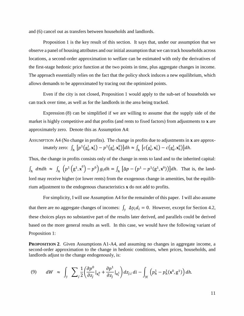
Proposition 1 is the key result of this section. It says that, under our assumption that we

observe a panel of housing attributes and our initial assumption that we can track households across

locations, a second-order approximation to welfare can be estimated with only the derivatives of

the first-stage hedonic price function at the two points in time, plus aggregate changes in income.

The approach essentially relies on the fact that the policy shock induces a new equilibrium, which

allows demands to be approximated by tracing out the optimized points.

Even if the city is not closed, Proposition 1 would apply to the sub-set of households we

can track over time, as well as for the landlords in the area being tracked.

Expression (8) can be simplified if we are willing to assume that the supply side of the

market is highly competitive and that profits (and rents to fixed factors) from adjustments to x are

approximately zero. Denote this as Assumption A4:

ASSUMPTION A4 (No change in profits). The change in profits due to adjustments in x are approx-imately zero: ∫ �𝜕𝜕1�gℎ

1, 𝐱𝐱ℎ1� − 𝜕𝜕1�gℎ1, 𝐱𝐱ℎ

0��𝑑𝑑ℎℎ ≈ ∫ �𝑐𝑐�gℎ1, 𝐱𝐱ℎ1� − 𝑐𝑐�gℎ

1, 𝐱𝐱ℎ0��𝑑𝑑ℎℎ .

Thus, the change in profits consists only of the change in rents to land and to the inherited capital:

∫ 𝑑𝑑π𝑑𝑑ℎℎ ≈ ∫ �𝜕𝜕1 �g1, 𝐱𝐱0� − 𝜕𝜕0� 𝑔𝑔𝑖𝑖𝑑𝑑ℎℎ = ∫ �∆𝜕𝜕 − �𝜕𝜕1 − 𝜕𝜕1(g1, 𝐱𝐱0)��𝑑𝑑ℎℎ . That is, the land-

lord may receive higher (or lower rents) from the exogenous change in amenities, but the equilib-

rium adjustment to the endogenous characteristics x do not add to profits.

For simplicity, I will use Assumption A4 for the remainder of this paper. I will also assume

that there are no aggregate changes of incomes: ∫ ∆𝑦𝑦𝑖𝑖𝑑𝑑𝑖𝑖 = 0ℐ . However, except for Section 4.2,

these choices plays no substantive part of the results later derived, and parallels could be derived

based on the more general results as well. In this case, we would have the following variant of

Proposition 1:

PROPOSITION 2. Given Assumptions A1-A4, and assuming no changes in aggregate income, a second-order approximation to the change in hedonic conditions, when prices, households, and landlords adjust to the change endogenously, is:

(9) 𝑑𝑑𝑊𝑊 ≈ � �12�𝜕𝜕𝜕𝜕0

𝜕𝜕𝑧𝑧𝑗𝑗|𝐳𝐳𝑖𝑖0 +

𝜕𝜕𝜕𝜕1

𝜕𝜕𝑧𝑧𝑗𝑗|𝐳𝐳𝑖𝑖1�𝑗𝑗

𝑑𝑑𝑧𝑧𝑗𝑗,𝑖𝑖ℐ

𝑑𝑑𝑑𝑑 − � �𝜕𝜕ℎ1 − 𝜕𝜕ℎ1(𝐱𝐱0, g1)�ℋ

𝑑𝑑ℎ.

12

Proof: The proposition follows immediately from applying Assumption A4 and ∫ ∆𝑦𝑦𝑖𝑖𝑑𝑑𝑖𝑖 = 0ℐ to Proposition 1.

Proposition 2 states that we can measure benefits by tracking the change in amenities ex-

perienced by each household, weighted by the average of the derivatives of the two hedonic price

functions evaluated at the households' choice, netting out any aggregate price changes that reflect

real costs of adjustments in x.

Note finally that in the simple case where there are no supply adjustments, then 𝑥𝑥𝑖𝑖(0),𝑟𝑟1 =

𝑥𝑥𝑖𝑖(0),𝑟𝑟0 and the entire expression collapses to

(10) 𝑑𝑑𝑊𝑊 ≈ � �12�𝜕𝜕𝜕𝜕0

𝜕𝜕𝑧𝑧𝑗𝑗|𝐳𝐳𝑖𝑖0 +

𝜕𝜕𝜕𝜕1

𝜕𝜕𝑧𝑧𝑗𝑗|𝐳𝐳𝑖𝑖1�𝑗𝑗

𝑑𝑑𝑧𝑧𝑗𝑗,𝑖𝑖ℐ

𝑑𝑑𝑑𝑑.

Expression (10) is just the individual household measure from Expression (4) summed over house-

holds, but with the ∆p terms cancelling as transfers between residents and landlords. It is similar

to the partial equilibrium measure recently suggested by Bishop and Timmins (2018).

Figure 1 illustrates this measure, or equivalently this portion of the Expressions (8) and (9).

The figure shows the derivatives with respect to g of both the t=0 and t=1 hedonic functions; these

derivatives are positive and continuous but unrestricted as to slope or curvature. The line bid(g)

represents the linearized approximation to the Marshallian marginal WTP function.7 The points

g0 and g1 represent the levels of the public good selected by the consumer in each scenario. Alt-

hough it is a Marshallian measure, the area under the linearized marginal WTP function represents

a second-order approximation to the welfare change associated with the change in equilibria. The

figure illustrates this measure only in the dimension of g, but note Expressions (8) to (10) require

summing over all attributes j. Even if there are no adjustments to x in the housing stock as a result

7 The interpretation of the Marshallian bid functions requires some nuance. As noted above, the marginal values for g are along a path where non-linear prices and, potentially, incomes are changing. Thus, it is not like a Marshallian demand curve at constant income. Even if incomes are constant, in the hedonic context, as other non-linear pricing contexts (e.g. Wilson 1993), the Marshallian quantity demanded of a character-istic depends on the entire price function, not just the marginal price at the quantity demanded. Consider a consumer at some optimal point in characteristic space. If there is now a shift in the infra-marginal portions of the hedonic price function, in a way that leaves the marginal prices unchanged, the consumer may still re-optimize because of the income effect associated with the infra-marginal expenditure. These and any other income effects are incorporated into the welfare measure derived in this paper.

13

of the policy, the welfare measure for this change in g still requires taking these terms into account,

weighted by the average marginal WTP of the household. The measures are no different if people

are owner-occupiers. In that case, the wealth effects still cancel and the dz terms incorporate the

wealth effects on demand for attributes, as would be appropriate. Regardless, a valid welfare

measure can be obtained simply by adding up experienced changes in characteristics, weighted by

the average marginal values.

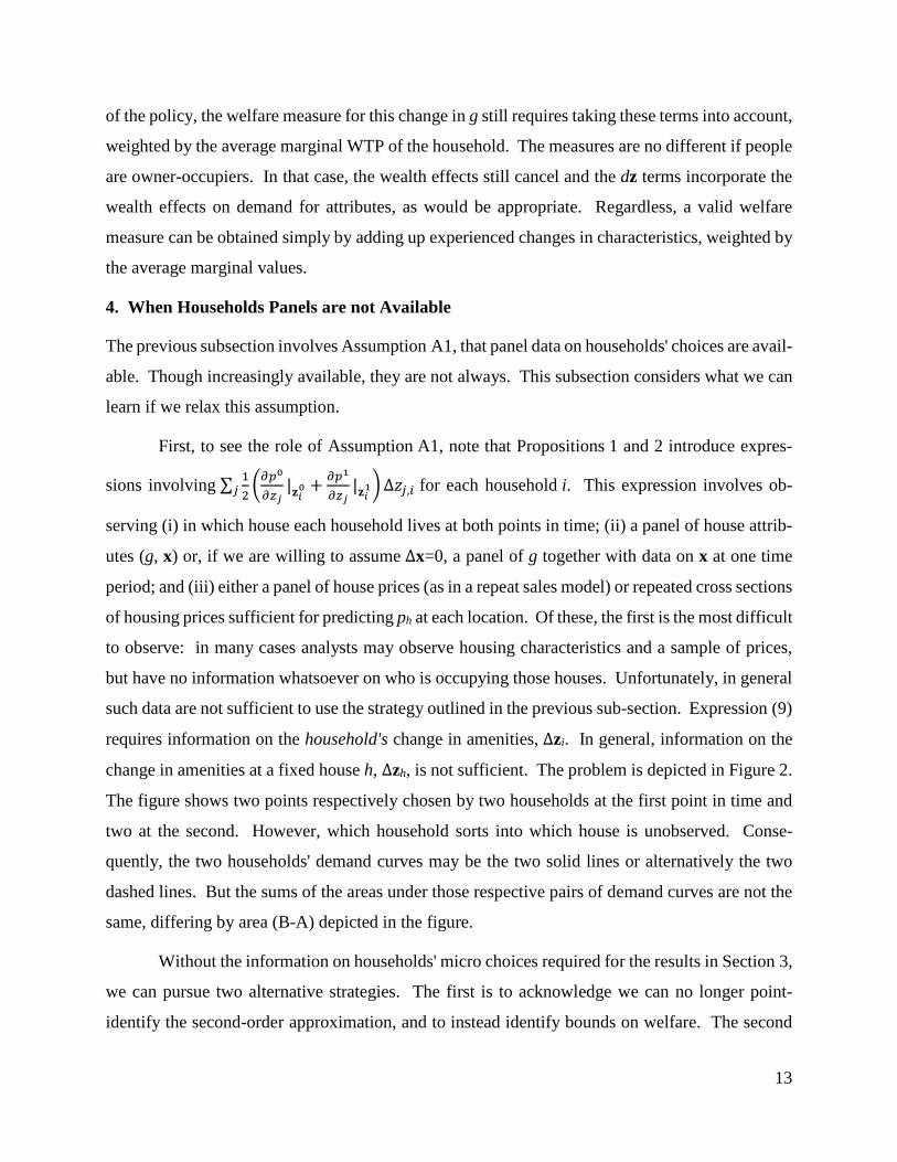
4. When Households Panels are not Available

The previous subsection involves Assumption A1, that panel data on households' choices are avail-

able. Though increasingly available, they are not always. This subsection considers what we can

learn if we relax this assumption.

First, to see the role of Assumption A1, note that Propositions 1 and 2 introduce expres-

sions involving ∑ 12�𝜕𝜕𝑝𝑝

0

𝜕𝜕𝑧𝑧𝑗𝑗|𝐳𝐳𝑖𝑖0 + 𝜕𝜕𝑝𝑝1

𝜕𝜕𝑧𝑧𝑗𝑗|𝐳𝐳𝑖𝑖1�𝑗𝑗 ∆𝑧𝑧𝑗𝑗,𝑖𝑖 for each household i. This expression involves ob-

serving (i) in which house each household lives at both points in time; (ii) a panel of house attrib-

utes (g, x) or, if we are willing to assume ∆x=0, a panel of g together with data on x at one time

period; and (iii) either a panel of house prices (as in a repeat sales model) or repeated cross sections

of housing prices sufficient for predicting ph at each location. Of these, the first is the most difficult

to observe: in many cases analysts may observe housing characteristics and a sample of prices,

but have no information whatsoever on who is occupying those houses. Unfortunately, in general

such data are not sufficient to use the strategy outlined in the previous sub-section. Expression (9)

requires information on the household's change in amenities, ∆zi. In general, information on the

change in amenities at a fixed house h, ∆zh, is not sufficient. The problem is depicted in Figure 2.

The figure shows two points respectively chosen by two households at the first point in time and

two at the second. However, which household sorts into which house is unobserved. Conse-

quently, the two households' demand curves may be the two solid lines or alternatively the two

dashed lines. But the sums of the areas under those respective pairs of demand curves are not the

same, differing by area (B-A) depicted in the figure.

Without the information on households' micro choices required for the results in Section 3,

we can pursue two alternative strategies. The first is to acknowledge we can no longer point-

identify the second-order approximation, and to instead identify bounds on welfare. The second

14

is to impose more structure. The following two sub-sections consider each strategy in turn.

4.1. Non-parametric bounds on welfare

As depicted in Figure 2, the fundamental problem when we do not observe a panel of households'

choices is that we do not know how to connect the points across equilibria. Choice patterns could

follow the dashed lines or the solid lines in the figure. However, a basic market clearing condition

is that they must connect in some way: all households are in a house in each period, and all houses

are occupied.

This basic insight suggests a way to bound welfare: simply search across all possible ways

to "connect the dots" and find those that yield the lowest welfare estimate and the highest welfare

estimate respectively. In particular, let ℋ and ℐ now be finite countable sets indexed by

h={1,…,H} and i={1,…,I} with H=I. In Figure 2, H=2, and there are two possibilities, the dashed

lines or the solid lines. In general, there are H! ways to connect the dots between H houses. How-

ever, this "search" can be solved with a simple linear program. Let 𝐼𝐼ℎ,ℎ′ be an indicator variable

for whether some household (hypothetically) lived in house h at t=0 and in house h' at t=1. We

then have the following proposition.

PROPOSITION 3. Under Assumptions A2-A4, a lower bound on aggregate welfare for a change in conditions, when prices, households, and landlords adjust to the change endogenously, can be found by solving the linear program:

𝑀𝑀𝑑𝑑𝑀𝑀{𝐼𝐼ℎ,ℎ′} �� � 𝐼𝐼ℎ,ℎ′�12�𝜕𝜕𝜕𝜕0

𝜕𝜕𝑧𝑧𝑗𝑗|𝐳𝐳ℎ0 +

𝜕𝜕𝜕𝜕1

𝜕𝜕𝑧𝑧𝑗𝑗|𝐳𝐳ℎ′1 �𝑗𝑗

�𝑧𝑧𝑗𝑗,ℎ′1 − 𝑧𝑧𝑗𝑗,ℎ

0 �ℎℎ′

−� �𝜕𝜕ℎ′1 − 𝜕𝜕ℎ′1 (𝐱𝐱0, g1)�ℎ′

�

such that

� 𝐼𝐼ℎ,ℎ′

ℎ= 1 ∀ ℎ′

� 𝐼𝐼ℎ,ℎ′ℎ′

= 1 ∀ ℎ.

An upper bound can be found by instead maximizing the objective. Proof: see the appendix.

Note the objective being minimized (or maximized) is the welfare approximation defined

by Expression (9), simply changing the points of evaluation to an arbitrary pair h,h', multiplying

by the indicator, and summing over both indices h and h'. The constraints represent the fact that

each house is only chosen once at each point in time.

15

4.2. Identification using single-crossing

An alternative to the bounds is to impose additional structure on the problem, namely a

"single-crossing" restriction on any two households' indifference curves. If we additionally as-

sume incomes are constant over time, then single crossing amounts to a restriction on preferences

such that households' Marshallian marginal WTP functions for some observed amenity do not

cross. That is, households can be ordered by their marginal WTP for the amenity, and the ordering

will be the same evaluated at any level of the amenity and under any equilibrium price function.

Because households always sort in the same order, if we have single crossing on g then in Figure 2

we can infer that the sorting is that of the dashed lines, ruling out the solid lines. Essentially, the

logic of single crossing provides a way to impute households' pattern of sorting, even when their

actual locations are not observed. This property is formalized in Assumption A5:

ASSUMPTION A5 (Single Crossing). Let Vji(yi, p( ), zj) be the indirect function conditional on one attribute zj given the price function p(), with the other attributes optimally chosen subject to zj, y, and p() to determine the utility level. Let ℐ be a simply ordered set and let the distri-

bution of demands be such that, for some amenity zj, 𝑣𝑣𝑖𝑖𝑡𝑡/𝜕𝜕𝑧𝑧𝑗𝑗 ≠ 0 ∀ i and 𝜕𝜕𝑉𝑉𝑗𝑗,𝑖𝑖�𝑦𝑦𝑖𝑖,𝑝𝑝( ),𝑧𝑧𝑗𝑗� 𝜕𝜕𝑧𝑧𝑗𝑗�𝜕𝜕𝑉𝑉𝑗𝑗,𝑖𝑖�𝑦𝑦𝑖𝑖,𝑝𝑝( ),𝑧𝑧𝑗𝑗� 𝜕𝜕𝑦𝑦⁄

is everywhere non-decreasing in i. Furthermore, either 𝑦𝑦𝑖𝑖 is constant over time, or utility is quasi-linear in y.

Assumption A5 requires single crossing in only one dimension of the characteristic space,

zj.8 A public good of particular interest like g may be a natural choice for that attribute, but that

choice is not necessary. It could be any characteristic or any scalar-valued index of characteristics.

Even though we are modeling multidimensional characteristics, induced assortative matching

along any one dimension is enough to impute households' choices. The single-crossing assump-

tion, sometimes called the Spence-Mirrlees condition when written this way, guarantees that the

level of zj chosen by households is always increasing in i. See, e.g., Milgrom and Shannon (1994)

and Athey, Milgrom, and Roberts (1998 Ch. 3) for proofs. To see this intuitively, note that we

could write A5 alternatively as follows. For any two households i, i' if 𝜕𝜕𝑉𝑉𝑗𝑗,𝑖𝑖�𝑦𝑦𝑖𝑖,𝑝𝑝�( ),�̂�𝑧𝑗𝑗� 𝜕𝜕�̂�𝑧𝑗𝑗�𝜕𝜕𝑉𝑉𝑗𝑗,𝑖𝑖�𝑦𝑦𝑖𝑖,𝑝𝑝�( ),�̂�𝑧𝑗𝑗� 𝜕𝜕𝑦𝑦⁄ ≥

8 As Chiappori, McCann, and Nesheim (2010) discuss, extensions of the single-crossing property to the multi-attribute case lose the interpretation of inducing assortative matching. Although we are working with a multi-attribute model, Assumption 5 involves single-crossing of the WTP functions in the dimension of only one attribute, not multiple attributes.

16

𝜕𝜕𝑉𝑉𝑗𝑗,𝑖𝑖′�𝑦𝑦𝑖𝑖′ ,𝑝𝑝�( ),�̂�𝑧𝑗𝑗� 𝜕𝜕�̂�𝑧𝑗𝑗�

𝜕𝜕𝑉𝑉𝑗𝑗,𝑖𝑖′�𝑦𝑦𝑖𝑖′ ,𝑝𝑝�( ),�̂�𝑧𝑗𝑗� 𝜕𝜕𝑦𝑦⁄ for some �̂�𝑧𝑗𝑗 , �̂�𝜕( ), then 𝜕𝜕𝑉𝑉𝑗𝑗,𝑖𝑖�𝑦𝑦𝑖𝑖,𝑝𝑝( ),𝑧𝑧𝑗𝑗� 𝜕𝜕𝑧𝑧𝑗𝑗�𝜕𝜕𝑉𝑉𝑗𝑗,𝑖𝑖�𝑦𝑦𝑖𝑖,𝑝𝑝( ),𝑧𝑧𝑗𝑗� 𝜕𝜕𝑦𝑦⁄ ≥

𝜕𝜕𝑉𝑉𝑗𝑗,𝑖𝑖′�𝑦𝑦𝑖𝑖′ ,𝑝𝑝( ),𝑧𝑧𝑗𝑗� 𝜕𝜕𝑧𝑧𝑗𝑗�

𝜕𝜕𝑉𝑉𝑗𝑗,𝑖𝑖′�𝑦𝑦𝑖𝑖′ ,𝑝𝑝( ),𝑧𝑧𝑗𝑗� 𝜕𝜕𝑦𝑦⁄ for all 𝑧𝑧𝑗𝑗 , p( ).

Thus, if a household selects more zj than another household in the baseline scenario, it will do so

in the ex post scenario as well.9 However, this requires ruling out income effects.

All this suggests a simple approach for identifying Expression (9) without panel data on

households. Let 𝐹𝐹𝑗𝑗𝑡𝑡( ) be the distribution function of some continuously distributed amenity zj at

time t. Given that zj is continuously distributed, for each observed percentile θ ∈ {1/H, 2/H, …,

1} of the distribution of zj, there will be a unique vector zt(θ) at t. Let 𝑧𝑧𝑘𝑘𝑡𝑡 (θ) be the value of the kth

attribute of this vector. Note that for k=j, 𝑧𝑧𝑘𝑘𝑡𝑡 (θ)=(𝐹𝐹𝑗𝑗𝑡𝑡)-1(θ). Then we can now state the following

proposition.

PROPOSITION 4. Under Assumptions A2-A5, aggregate welfare for a change in conditions, when prices, households, and landlords adjust to the change endogenously, can be computed from ob-served prices and estimated derivatives as follows:

(11) 𝑑𝑑𝑊𝑊 ≈ � �

12�𝜕𝜕𝜕𝜕0

𝜕𝜕𝑧𝑧𝑘𝑘|𝐳𝐳0(𝜃𝜃) +

𝜕𝜕𝜕𝜕1

𝜕𝜕𝑧𝑧𝑘𝑘|𝐳𝐳1(𝜃𝜃)�

𝑘𝑘[𝑧𝑧𝑘𝑘1(𝜃𝜃) − 𝑧𝑧𝑘𝑘0(𝜃𝜃)]

𝜃𝜃

−� �𝜕𝜕ℎ1 − 𝜕𝜕ℎ1(𝐱𝐱0, g1)�ℎ

Proof: Consider the initial equilibrium described by the hedonic price function p0(g, x). For any θ ∈ [1/H, 2/H,…,1], consider a household which chooses zj in the initial equilibrium such that 𝐹𝐹𝑗𝑗0(zj)=θ. By Assumption A5 (single crossing), when facing the new equilibrium price function p1(g, x), the household would choose zj such that 𝐹𝐹𝑗𝑗1(zj)=θ. The remainder follows by Proposi-tion 2, simply evaluating each household at the z corresponding to a constant percentile of the distributions of zj.

Proposition 4 states that one can rank the houses by one amenity zj in each scenario, find

the change in all attributes at a constant percentile of the zj distribution, and evaluate the derivatives

of the hedonic price function at the z falling at this percentile of the zj distribution. The final term

is the same price adjustments as in Expression (9). In practice, note that as long as one knows the

9 Intuitively, given that the Marshallian demand functions do not cross, this obviously must be so if the implicit price of zj is increasing in zj (i.e. if the hedonic price function is convex in zj). However, even if the implicit price is decreasing in zj over portions of the range, the second-order condition for utility maxi-mization requires that it cut the demand curves from below. In other words, the economics of the model require that the slope of the price function be greater than the slope of the demand curve in the neighborhood of the optimal choice. Thus, households will always "sort" across zj in the same order, even if they are changing consumption of other attributes or the numeraire.

17

attributes at all locations and time periods, this estimate can be implemented with only a repeated

cross section of housing prices (i.e. without a full panel): all that is required is that p1 and 𝜕𝜕𝑝𝑝𝑡𝑡

𝜕𝜕𝑧𝑧𝑗𝑗 can

be predicted for each house from the hedonic pricing model.

This single-crossing condition is routinely imposed in the literature on non-linear pricing

(e.g. Athey, Milgrom, and Roberts 1998, Wilson 1993), including models of monopoly screening

as well as locational sorting. Although imposing this property is undoubtedly a restriction relative

to the more general treatment up to this point, it is actually less restrictive in this respect than many

structural models, which employ the same single crossing property plus additional functional form

restrictions or parametric restrictions on the distribution of unobservable demand shifters. For

example, consider the common class of models which allow households i to differ in two dimen-

sions, income y and a parameter α reflecting tastes for g. Many hedonic and sorting applications,

including Bajari and Benkard (2005), Heckman, Matzkin, and Nesheim (2010b), and Bishop and

Timmins (2019) impose the additional restriction that WTP is strictly increasing in α and that

preferences are quasi-linear. These models implicitly impose Assumption A5: households are

totally ordered by α, with increasing α implying increasing g.

This is not to say that all papers impose these conditions. Other models impose only a

partial ordering on i rather than a total ordering. For example, Sieg et al. (2004), Epple, Peress,

and Sieg (2010), and Kuminoff (2012) order households by α conditional on y, and vice versa.

However, pairs of households where one has higher α and the other higher y need not be ordered:

one household may choose higher g than the other household in one equilibrium but not necessarily

in another equilibrium. In this sense, Assumption A5 is stronger than the related single crossing

assumptions imposed in those papers. However, in other respects the approach of this section still

imposes weaker assumptions about heterogeneity. Sieg et al. (2004), Epple, Peress, and Sieg

(2010), and Kuminoff (2012) compensate for their weaker single crossing assumptions by impos-

ing additional functional form restrictions on v() and/or parametric assumptions on the joint distri-

bution of (α, y).

Of course, single crossing is only a modeling assumption. In practice, Expression (11) may

be a reasonable approximation to Expression (9) even when households are not truly totally or-

dered, in violation of Assumption A5. In the simulations reported in Section 7, the matching-by-

percentiles approach of Expression (11) gives results quite close to the matching-by-households

18

approach of Expression (9), even when households are not totally ordered. To see why, note that

if the hedonic price functions were linear, so that marginal prices were constant, then any matches

would give the same aggregate welfare measures, namely the average of the two marginal values

times the sum of changes in the attributes. So, when single crossing does not hold, even if house-

holds do not sort in exactly the same order in different scenarios, their rank orderings are still

correlated. Consequently, violations of Assumption A5 create errors in the imputation of z that

are only local. If the hedonic price functions is approximately linear over the range of the errors,

then the errors offset (with area A approximately equal to area B in Figure 2). In this sense, esti-

mates based on Expression (11) can be thought of as approximations to Expression (9).

4.3 Matching by group

Whereas Section 3 assumed complete knowledge about where individual households sort

over time in the product space, this section so far has assumed no knowledge about that whatso-

ever. In between these two cases are a variety of intermediate ones where partial information is

available on the households locating at a house. Such partial information would allow us to either

further restrict the bounds of Section 4.1 by ruling out some possible matches, or alternatively to

partially relax the single-crossing assumption of Section 4.2.

For example, suppose we can track where types of households live but not the individual

household. Perhaps we can observe the race of a household occupying a given house, or its in-

come, or some other characteristic or combination of characteristics. Then the bounds of Sec-

tion 4.1 can be tightened by imposing the additional restriction that 𝐼𝐼ℎ,ℎ′ = 0 whenever the observed

characteristics of households at h in t=0 and h' in t=1 do not correspond.

Alternatively, the structure imposed in Section 4.2 can be relaxed, as we would now only

require that the single crossing property hold within observable type. In particular, the required

single-crossing condition may be modified as follows.

ASSUMPTION A5' (Single crossing within type). Let 𝒯𝒯 be a set of observable types which partitions the set of households H. Let τ ⊂ 𝒯𝒯 be the set of households of a specific type with measure µτ, ∑τµτ=1, and let each τ be a simply ordered subset of the partially ordered set ℐ. For each τ, let the distribution of demands be such that, for some amenity zj, at fixed 𝑦𝑦𝑖𝑖 , 𝜕𝜕𝑉𝑉𝑗𝑗,𝑖𝑖�𝑦𝑦𝑖𝑖,𝑝𝑝( ),𝑧𝑧𝑗𝑗� 𝜕𝜕𝑧𝑧𝑗𝑗�𝜕𝜕𝑉𝑉𝑗𝑗,𝑖𝑖�𝑦𝑦𝑖𝑖,𝑝𝑝( ),𝑧𝑧𝑗𝑗� 𝜕𝜕𝑦𝑦⁄ is everywhere nondecreasing in i ∈ 𝜏𝜏.

This property guarantees that, after conditioning on the observed type, households sort along zj in

19

the same order. Thus, if a household selects more zj than another household of the same type in

the baseline scenario, it will do so in the ex post scenario as well. This approach allows households

to be partially ordered overall but totally ordered within type, as in the Epple-Sieg approach, where

households are totally ordered after conditioning on income.

In this case, Expression (11) can be modified as follows. Let Iτ be the number of observed

households of type τ and let θτ={1/Iτ, 2/Iτ,…,1} be the observed percentiles of the distribution of

zj among type τ. Then by the same argument as given in Proposition 4, aggregate welfare is

(12) 𝑑𝑑𝑊𝑊 ≈ �

𝜇𝜇𝜏𝜏𝐼𝐼𝜏𝜏� �

12�𝜕𝜕𝜕𝜕0

𝜕𝜕𝑧𝑧𝑘𝑘�𝐳𝐳0(𝜃𝜃𝜏𝜏) +

𝜕𝜕𝜕𝜕1

𝜕𝜕𝑧𝑧𝑘𝑘� 𝐳𝐳1(𝜃𝜃𝜏𝜏)�

𝑘𝑘[𝑧𝑧𝑘𝑘1(𝜃𝜃𝜏𝜏) − 𝑧𝑧𝑘𝑘0(𝜃𝜃𝜏𝜏)]

𝜃𝜃𝜏𝜏𝜏𝜏∈𝒯𝒯

−� �𝜕𝜕ℎ1 − 𝜕𝜕ℎ1(𝐱𝐱0, g1)�𝐻𝐻

That is, for each type, one can take the set of houses occupied by that type and rank them by zj in

both scenarios, find the change in zk at a constant percentile of the distribution, and evaluate the

derivatives of the hedonic price function at the same percentile of the distribution. Then, one can

take the weighted sum over types. Moreover, if the type is observed income, then we no longer

need to rule out income effects, as we can condition on them.

5. Transactions Costs

So far, we have assumed that there are no transactions costs from re-optimizing (Assumption A2).

This assumption may be most fitting for consumer goods such as computers (Bajari and Benkard

2005) or groceries (Griffith and Nesheim 2013), which are purchased regularly. For applications

to housing or to labor markets, the transaction costs of moving homes or changing jobs may be

much higher.

With transactions costs, Propositions 1 and 2 are no longer valid, because the first-order

condition of utility maximization represented by Equation (1) no longer need hold in both periods

(see Bishop and Murphy 2019 for discussion). Instead, the transactions costs create a wedge,

turning the equalities of Equation (1) into inequality constraints.

However, we can still bound the results. First, return to the case where Assumption A1

holds, so we observe whether households move or not. In addition, suppose that households my-

20

opically optimized in the baseline period (without anticipating changes). Finally, suppose the an-

alyst has an estimate of the average moving cost among those who actually move, MC. (Alterna-

tively, we can always make what-if statements along the lines of: "if average moving costs are MC,

then the bounds would be such-and-such.")

For movers, we then can still use Propositions 1 or 2 to form point estimates of their wel-

fare, subtracting out aggregate moving costs, which is MC times the number of movers. For non-

movers, when conditions improve, we can create an upper bound on compensating variation by

assuming constant marginal WTP from the baseline condition. Essentially, this uses a rectangle

instead of the trapezoid. By the same token, for non-movers we can create a lower bound of zero.

When conditions worsen instead of improve, the rectangle at baseline marginal WTP is now a

lower bound on damages. Adding up the welfare for the movers and non-movers creates a bound

for the whole group. The bound involves a mix of first-order approximations and second-order

approximations suited to the situations observed.

If, instead of being myopic, households are forward-looking, then the recent results of

Bishop and Murphy (2019) apply. They develop a model in which households make a single

choice of a house to which they're committed. Households maximize expected utility at the house,

given the current price functions and expectations about future amenities. To see the connection

between the Harberger approximation and their results, suppose, momentarily, that households are

not only forward-looking but perfectly prescient about the future and, furthermore, that WTP func-

tions for amenities are linear. Then, in the model of Bishop and Murphy, households would set an

average of (discounted) marginal WTP over time equal to the marginal hedonic price at the time

of purchase, and Lemma 1 above would hold exactly if we applied a discount rate to the second

period terms. Essentially, the conditions holding across two time periods with no transactions cost

are the same as the conditions that hold at a single point in time when there are transactions costs.

As Bishop and Murphy show, when households are not perfectly prescient but still right "on aver-

age," the hedonic estimate would still be unbiased when amenities are increasing or decreasing.

They further show that when WTP functions are non-linear, there is a bias from a static hedonic

model. The results of this paper can be applied to their bias term to suggest that the bias is third-

order.

Next, relax Assumptions A1 and A2, so that there are moving costs and we do not observe

21

household movements. Unfortunately, the lower bound from the linear program of Proposition 3

is no longer valid, because with moving costs we can no longer assume that the quantities de-

manded even trace out a demand curve at all, even the demand curves implied by the lower-bound

algorithm.

However, the upper bound from Proposition 3 does remain valid. The intuition here is

simple: By Proposition 3, the expression is an upper bound on welfare when there are no moving

costs. Because moving costs can only reduce the true welfare of a change in the economic envi-

ronment, the expression remains an upper bound. This result is quite general.

Moreover, it may be possible to find tighter bounds. In particular if a household is assumed

to move from h to h', it must be that they are willing to pay the transactions cost to move to h'

rather than stay in h under the new conditions, given the preferences implied by the move from h

to h'. Accordingly, if we know individual MC (or assume homogeneous moving costs), we can

impose the additional restriction in the linear problem associated with Proposition 3:

𝐼𝐼ℎ,ℎ′

⎣⎢⎢⎢⎡

�

⎝

⎜⎜⎛1

2𝜕𝜕𝜕𝜕1

𝜕𝜕𝑧𝑧𝑗𝑗|𝐳𝐳ℎ′1 +

12

⎝

⎜⎛𝜕𝜕𝜕𝜕1

𝜕𝜕𝑧𝑧𝑗𝑗|𝐳𝐳ℎ′1 +

𝜕𝜕𝜕𝜕1𝜕𝜕𝑧𝑧𝑗𝑗

|𝐳𝐳ℎ′1 − 𝜕𝜕𝜕𝜕0𝜕𝜕𝑧𝑧𝑗𝑗

|𝐳𝐳ℎ0

𝑧𝑧𝑗𝑗,ℎ′1 − 𝑧𝑧𝑗𝑗,ℎ

0 �𝑧𝑧𝑗𝑗,ℎ′1 − 𝑧𝑧𝑗𝑗,ℎ

1 �

⎠

⎟⎞

⎠

⎟⎟⎞

𝑗𝑗�𝑧𝑧𝑗𝑗,ℎ′

1 − 𝑧𝑧𝑗𝑗,ℎ1 �

− �𝜕𝜕ℎ′1 − 𝜕𝜕ℎ1� − 𝑀𝑀𝑀𝑀

⎦⎥⎥⎥⎤

≥ 0 ∀ ℎ, ℎ′ ≠ ℎ

The ratio �𝜕𝜕𝑝𝑝1

𝜕𝜕𝑧𝑧𝑗𝑗|𝐳𝐳ℎ′1 − 𝜕𝜕𝑝𝑝0

𝜕𝜕𝑧𝑧𝑗𝑗|𝐳𝐳ℎ0� �𝑧𝑧𝑗𝑗,ℎ′

1 − 𝑧𝑧𝑗𝑗,ℎ0 �� gives the slope of the demand curve implied by

the move from h at t=0 to h' at t=1. The terms 𝜕𝜕𝑝𝑝1

𝜕𝜕𝑧𝑧𝑗𝑗|𝐳𝐳ℎ′1 and the large term in parentheses are the

height of this demand curve evaluated respectively at h' and h at t=1. Multiplying by the actual

difference in z and subtracting the price difference gives the consumer surplus. Multiplying by

𝐼𝐼ℎ,ℎ′, this restriction insures that either 𝐼𝐼ℎ,ℎ′=0, or else the consumer surplus of moving from h to

h' exceeds transactions costs.

22

6. When Preferences Shift

In all the models to this point, we have relied on Assumption A3, that households' preferences are

constant over the time period considered, so that a household's optimal choice of the vector z is an

unchanging functional of the hedonic price function and income. As with Assumption A2 (moving

costs), Assumption A3 may be most fitting for hedonic applications to consumer goods such as

computers or groceries. It may be less fitting for applications to housing if taste changes are im-

portant in that context or, to put it differently, when there are important changes in parameters

affecting current-period utility, such as family status. In such cases, even when we observe points

for two equilibria for a single household (Section 3), they may be on two different utility functions.

Likewise, even if household preferences exhibit the single crossing property (Section 4), if prefer-

ences are shifting then there is no reason to believe households are still sorting in the same order.

In this section, I consider relaxing Assumption A3 as well as Assumption A1. That is, we

do not observe a panel of households and, moreover, an individual's household's WTP for attributes

may be changing anyway. Such changes in demands of course will have implications for equilib-

rium hedonic prices. But more importantly, they raise fundamental questions about what perspec-

tive to take when evaluating changes in conditions (Stapleford 2009). I take the approach of Fisher

and Shell (1972) and Pollak (1989), who suggest that welfare comparisons can be made in such

situations from the perspective of one or the other of the two preference relationships. This basic

approach also is implicit in simulation exercises such as those in Sieg et al. (2004), Bayer et al.

(2011), or elsewhere, where general equilibrium welfare effects are estimated for policy shocks

under an assumption of constant preferences, even though preferences may well change over the

time periods envisioned. Essentially, these simulations evaluate the policy shocks from the per-

spective of ex ante preferences.

From this perspective, we can again use the single crossing property along with a weaker

version of Assumption A3:

ASSUMPTION A3'. The distribution of pairs (vt(), yt) is the same as it would have been if v() were constant. Consequently, the distribution of demand functionals z(pt( )) is the same.

Assumption A3' is implied by A3 but not the reverse. It says that although individual households'

demand functions may change over time, the distribution of demand types remains constant. This

assumption is probably most valid for short time windows, such as those considered by Figlio

23

(2004), Lucas (2004), or the 1999-2000 change in crime recently considered by Bishop and Tim-

mins (2019).

With this weaker assumption, all the results of Section 4 flow through, but now interpreting

the result as the welfare measure from the perspective of a single time period. For example, when

single crossing holds, we can now state Proposition 5.

PROPOSITION 5 Under Assumptions A2, A3' and A4-A5, aggregate welfare for a change in he-donic conditions, evaluated from the perspective of constant preferences for each household, can be computed from observed prices and estimated derivatives as given by Equation (11). Moreover, the aggregate evaluation is the same whether using ex ante or ex post preferences (though the distributional effects may be different).

Proof: See the appendix.

Proposition 5 says that we can still use the same measure for aggregate welfare as given in

Proposition 4 under a weaker version of Assumption A3, in which individual household demands

may shift due to changes in preferences or incomes, as long as the distribution of demands does

not change. However, the welfare estimates are now from a single period perspective, or alterna-

tively are counterfactual estimates "as if" preferences had remained constant.

The intuition of Proposition 5 is fairly straightforward. We wish to estimate welfare "as

if" preferences had not changed between periods. However, if the joint distribution of preferences

and incomes are the same as if preferences hadn't changed, the observed equilibria are the same as

they would have been under the missing hypothetical. Therefore, any welfare measures we con-

struct from the observed equilibria are consistent with what we'd want under the missing hypo-

thetical.

Moreover, if single crossing is considered too strong an assumption, we can still construct

the bounds of Section 4 by the same argument.

7. Illustrative Simulations

In this section I illustrate the results from the previous two sections using simulated data, which

allows us to compare the constructs to "true" welfare values. In particular, I simulate 100 hedonic

housing equilibria, each with 1000 households and 1000 houses. Households sort over two varia-

bles, a lot of fixed size with an exogenously supplied amenity g, which is shocked between two

time periods, and housing capital x, which is sold endogenously by suppliers. Households update

24

their purchase of x between scenarios.

The public good g is uniformly distributed on (1, 3) in the baseline scenario. In the ex post

scenario, one-third of the houses are treated by a policy. If a house is treated, its level of g improves

such that g1 = g0 + (3-g0)/3 + 1. Panel A of Figure 3 illustrates the levels of g in one representative

simulation. It shows the cumulative distribution functions (CDF) of g in each scenario, indicating

that the ex ante scenario is uniformly distributed, while the ex post scenario, which 1st-order sto-

chastically dominates it, is not.

I use two functional forms for utility. First, I use a functional form introduced by Epple

and Sieg (1999), variants of which have been used by Sieg et al. (2004), Epple, Peres, and Sieg

(2010), Kuminoff (2012), and others. In particular, indirect utility is given by:

(13) 𝑉𝑉 = �𝛼𝛼g𝜌𝜌 + �e(𝑦𝑦−𝑝𝑝(g))1−𝜈𝜈−1

1−𝜈𝜈 e−𝛽𝛽𝑝𝑝𝑥𝑥

𝜂𝜂+1−1𝜂𝜂+1 �

𝜌𝜌

�

1𝜌𝜌

where y is income, p(g) is the hedonic price of a lot with public good g, 𝜕𝜕𝑥𝑥 is the supply-price of

x, 𝛼𝛼 is an individual-specific taste parameter for g, and 𝛽𝛽, 𝜂𝜂, 𝜈𝜈, and 𝜌𝜌 are additional parameters.

This indirect utility function has no closed form for utility, but one can interpret it as involving a

constant-elasticity of substitution between private and public goods, and a constant income and

price elasticity of demand for x. With this model, demand for x is independent of g, except through

the effect of g on prices. I set 𝛽𝛽 = 3, 𝜂𝜂 = -0.963, 𝜈𝜈 = 0.75, and 𝜌𝜌 = -0.02. I let income be distributed

log-normal with μy = 11.1 and σy = 0.4 (and truncated at $25,000 and $200,000). Finally, I let 𝛼𝛼

be log-normal with μα = -0.25 and σα = 0.97. Single crossing does not strictly hold in this model,

though it holds in 𝛼𝛼 conditional on y and vice versa.

Second, I use the cross-packaging model, discussed and analysed by von Haefen (2007).

In particular, I assume indirect utility is given by:

(14) 𝑉𝑉 =

𝑦𝑦 − 𝜕𝜕(g) + 𝜃𝜃 ln(g)

exp �exp(𝛼𝛼 + 𝛿𝛿g)𝜕𝜕𝑥𝑥1+𝛽𝛽

1 + 𝛽𝛽 � .

25

In this model, g enters utility in two places. It enters as an additively separable term in the numer-

ator. It also enters in the denominator, in a term that shifts the demand for x. In particular, the

demand for x is given by:

(15) 𝑥𝑥∗ = 𝛼𝛼 + 𝛽𝛽ln(𝜕𝜕) + ln(𝑦𝑦) + 𝛿𝛿𝑔𝑔.

Thus, g is valued directly as well as indirectly through increasing the consumer surplus for x. I let

𝛼𝛼 ~u(-2.2, -1.8), 𝛽𝛽 = -1.1, 𝜃𝜃 ~u(750, 1050), and 𝛿𝛿 distributed triangular with points (0.004, 0.006,

0.012). Income is distributed as before. These parameters are calibrated so that the median mar-

ginal willingness to pay for g is approximately equal to that from the first model.

Given the distribution of g and of household characteristics, market-clearing prices were

solved for, along with equilibrium levels of the endogenous characteristic x, for each of the 100

simulations and for each utility function. Panel B of Figure 3 shows land prices, after netting out

the value of capital x, for one representative scenario using the Epple-Sieg utility function. It

shows that price levels increased in the ex post scenario. However, as scene in Panel C, marginal

prices (or marginal WTP) for g fell in the ex post scenario, largely because of the increased supply

of g. The marginal price function is quite convex, with an extremely sharp up-turn in the right-

hand tail.

Equilibrium prices in each scenario were then perturbed by an error term, normally and

independently distributed and calibrated such that the standard deviation of the error was equal to

1% of the mean price. This error term can be interpreted as either measurement error in price (the

dependent variable) or as an unobserved characteristic of the home that enters preferences as a

perfect substitute for the numeraire good.

Hedonic price functions were fitted to this noisy data using three methods. The first uses

semi-parametric methods, partially out x using linear regression and estimating the residual price

as a function of g using quadratic local regressions. The second uses a fifth-ordered polynomial

function. The third uses a translog function, regressing logged prices on logs of g and x, their

squares, and an interaction. Figure 4 shows the estimated partial derivatives with respect to g,

plotted against the true marginal WTP, for one representative simulation, for both the ex ante and

ex post scenarios, for the Epple-Sieg utility function. The local regression and the polynomial are

able to fit the data over most of the support, but badly under-predict in the right-hand tail, as they

26

cannot fit the sharp turn seen in Figure 3C. Nevertheless, those mistakes are over a range of the

data with little density, so the functions capture mean marginal values well. The translog function

does a much poorer fit overall, finding some negative values at low levels of g. It also does a poor

job of adjusting for changes in x. The equilibrium value of capital is separable in this model, but

the log transformation forces interactions in the value of g and x.

Finally, from these price functions and their derivatives, true welfare measures and the

empirical approximations were computed. Table 1 reports the results for baseline models, with no

transactions costs. The table shows mean values across the 100 simulations, as well as the 5th and

95th percentiles across simulations. The first two rows show the Hicksian CV and EV for the

improvement to g. EV is lower than CV in these scenarios because of the increase in prices, which

actually puts households on lower indifference curves. (However, net welfare still increases be-

cause these price increases are income to landlords.) The difference between EV and CV is greater

for the Epple-Sieg model at these parameter values.

In the third row, the table shows the value of Equation (9), when households can be tracked

over time. The first column computes the expression using the true marginal values from the utility

function. It shows that the second-order approximation falls between EV and CV, as expected.

The next columns compute the expression using the derivatives from the three respective estimated

price functions. With both utility functions, the semi-parametric and polynomial gradients do quite

well, giving values close to those using the true marginal values and close to the range of EV and

CV. The translog function badly overstates the values.

The remaining rows show the results from Section 4, which is applicable when households

cannot be tracked over time. The first two rows give the lower and upper bound respectively,

using a linear program to find the allocations over time that respectively minimize and maximize

total welfare. By construction, the values bracket those using Equation (9). They also bracket the

true EV and CV, with a reasonable range, again except for the translog function. The final row

shows the results when consumption patterns over time are imputed using the single crossing prop-

erty. Although the Epple-Sieg utility function does not impose single-crossing globally, house-

holds tend to sort in similar patterns over time. As a consequence, the errors from imposing single

crossing tend to be small and to cancel out. The welfare estimates using this imputation are almost

exactly the same as those constructed under the assumption that we can actually track households

27

over time.

To explore the reasons for this result, Figure 5 illustrates the sorting patterns observed in

one illustrative simulation. The first panel shows the level of g households choose in the ex post

scenario, against the marginal WTP for g of each household evaluated at the "average house."

That is, it shows the household's optimal g as a function of an index of its demand-type for g. If

bid functions never crossed, this figure would show an increasing function. While it is not strictly

increasing, it is nearly so, indicating the any crossings in the bid functions are only very local. The

second panel shows the households' level of g in the ex post scenario versus the ex ante scenario.

It illustrates that households sort approximately in the same order, though not exactly. Finally, the

third panel shows the level of g imputed for a household in the ex post scenario using single-

crossing, against its actual level of g in the scenario. It shows that the errors from imposing the

single-crossing assumption are fairly small. Consequently, the hedonic price function is approxi-

mately linear over the range of these errors, and the overall bias is minimal. Thus, even when

household sorting is not observed, and even when the single crossing property does not truly hold,

models based on this property potentially can still be quite useful.

Tables 2A and 2B report the results from imposing transactions costs in the equilibrium.

In particular, from an initial optimal point, households adjust to the shock in g subject to a moving

cost annualized to be $200 and $400 respectively in the two tables, which, at a 5% discount rate,

equate to one-time costs of $4,000 and $8,000. The true EV and CV are lower in these scenarios,

as households can no longer take advantage of the shock by re-optimizing as easily, and as real

resources are used up on transactions. Moreover, Equation (9) is no longer valid, as there is now

a wedge between the hedonic gradient and marginal values. As shown in the tables, the expression

gives values that now fall outside the range of EV and CV.

However, as discussed in Section 5, when we can track households, we can bound the true

values using a mix of first-order approximations for non-movers and Equation (9) for movers (net

of transactions costs). The fourth and fifth rows of the table show these results. Finally, when

households are not observed over time, we can still use the upper bound from Section 4, and even

tighten it somewhat by requiring the gain from any move to exceed transactions costs. The final

two rows in the table illustrate these bounds. The bounds are fairly tight in the simulations using

the Epple Sieg utility function, but are somewhat higher using the repackaging model.

28

8. Empirical Application and Comparison

To illustrate how the methods introduced in this paper can be used on real-world data, and to

compare the results to estimates from other structural models, I apply the methods to data previ-

ously studied by Bishop and Timmins (2019). They consider the value of reductions in violent

crime in the San Francisco area between 1999 and 2000. Over that period, average violent crime

rates fell by about 1.7%, though they increased at about one-third of housing locations.

Using housing data from 1994-2000, Bishop and Timmins estimate hedonic gradients for

crime, first partialling out the effects of structural characteristics, then estimating the gradient for

crime using local polynomial regression. They then estimate demand curves using Rosen's (1974)

two-step method, regressing marginal values from the first-stage price function on the level of

crime plus household level variables, including income and race, and year dummies (interpreted

as annual demand shifters). They also introduce a new maximum likelihood method in the spirit

of Heckman et al. (2005). This approach involves parameterizing utility, including unobserved

heterogeneity, and re-writing the problem to isolate the unobserved heterogeneity as a function of

marginal prices, crime and other observables, and the parameters. Values of the parameters that

maximize the likelihood can then be computed. See Bishop and Timmins (2019) for details.

Households are not tracked over time in these data. However, using the hedonic gradients

and crime levels, one easily can compute the values of Equation (11), using the single crossing

assumption. One need only sort the data by the 1999 crime level (or other attribute), then by the

2000 crime level, and merge the data back together. Averaging the 1999 and 2000 gradients and

multiplying by the change in crime gives the value of Equation (11).10 Table 3 gives the results.

The average value for the shift from the 1999 equilibrium to the 2000 equilibrium, including both

the change in crime and the shift in the hedonic price function, is $236. As discussed in Section 4,

instead of imposing single crossing, one can solve the linear program to bound the possible values.

The bounds using this approach are $235 to $568. Interestingly, in this application the single-

crossing approach identifies a point quite near the lower bound, unlike with the above simulations.

In general, where the single crossing estimate fits within the bounds will depend on the correlations

between changes in marginal prices and changes in amenities in the data.

10 Because the price effect of x is assumed to be linear, the terms involving it in Expression (11) cancel.

29

These results can be adjusted to make them more comparable to the results of Bishop and

Timmins (2019). In particular, Bishop and Timmins estimate a shift in demand for amenities

between 2019 and 2000 and then net out that shift in their welfare estimates (evaluating changes

from the 2019 perspective, not unlike the proposal in Section 6 above). They also cut off changes

in crime at a point where their estimated marginal willingness to pay falls to zero. For comparison

purposes, I adjust the 2000 marginal values downward by their estimated 2019-20 difference in

marginal values and use the same change in crime as they use after censoring. These adjusted

values are shown in the next three rows of the table. The average values fall by about $50.

Interestingly, these adjusted values are quit close to those using the more structural ap-

proach of Rosen (1974), as reported by Bishop and Timmins (2019). This suggests it may be

possible to approximate the results from more structural approaches using much simpler, reduced

form methods. Whereas the approach based on Equation (11) matches marginal values over time

based on a single crossing assumption, Rosen's approach essentially matches them over time by

matching on observed demographics. In this case, the results are quite similar. On the other hand,

at an average value of -$156, the new approach of Bishop and Timmins gives a very different

value. They find very negative values for the one-third of households who experience an increase

in violent crime, which more than offset the gains to other households. This difference is most

likely because the two approaches answer different questions. Whereas the approach suggested in

this paper values a change between general equilibria, including price changes, their approach

isolates the partial equilibrium value of a change in crime, netting out price effects.11

9. Conclusions

For decades, economists have used the hedonic model to estimate demands for the implicit char-

acteristics of differentiated commodities, including the demands for otherwise unpriced local pub-

lic goods and amenities. The traditional cross-sectional approach to hedonic estimation has recov-

ered marginal WTP for amenities when unobservables are conditionally independent of the amen-

ities, but has faltered over a difficult endogeneity problem when attempting non-marginal welfare

measures. In this paper, I show that when marginal prices can be reliably estimated, and when

panel data on household sorting is available, one can construct an approximation—using only the

first-stage marginal prices—which is a "sufficient statistic" for non-marginal welfare measures.

11An additional difference is that I use only 1999-2000 data, whereas they use the full 1994-2000 data set.

30

With this approximation, Rosen's second-stage estimation can be replaced with a simple average

of first-stage parameters.

Moreover, even when panel data on household sorting are unavailable, the sufficient sta-

tistic approach can be used to create bounds on the welfare measures using only repeated cross

sections of housing data. Alternatively, point identification can be established using a single cross-

ing restriction. In practice, this approximation appears to perform well in these simulations even

when this restriction does not strictly hold.

Future work might consider hybrids between the approach taken here and other work. Per-

haps the approach introduced here could be used to model baseline heterogeneity, while more

structural approaches could be introduced to model changes in preferences, semi-parametrically.

Perhaps it could be combined with quasi-experimental methods for identifying the hedonic price

function in panel data settings (Kuminoff and Pope 2014, Banzhaf 2018). Finally, perhaps it can

be combined with dynamic models to approximate or bound welfare when households anticipate

future changes (Bishop and Murphy 2019).

31

References

Athey, S., P. Milgrom, and J. Roberts. 1998. Robust Comparative Statics. Draft monograph available at scholar.harvard.edu/files/athey/files/draftmonograph98.pdf.

Bajari, P., and L. Benkard. 2005. Demand Estimation with Heterogeneous Consumers and Un-observed Product Characteristics: A Hedonic Approach. Journal of Political Economy 113(6): 1239-76.

Banzhaf, H.S. 2005. Green Price Indices. Journal of Environmental Economics and Management 49(2): 262-80.

Banzhaf, H.S. 2010. The Chicago School of Welfare Economics. In The Elgar Companion to the Chicago School of Economics, ed. by R. Emmett. Cheltenham, UK: Elgar, pp. 59-69.

Bartik, T.J. 1987. The Estimation of Demand Parameters in Hedonic Price Models. Journal of Political Economy 95(1): 81-8.

Bartik, T.J. 1988. Measuring the Benefits of Amenity Improvements in Hedonic Price Models. Land Economics 64(2): 172-83.

Bayer, P., M.D. Casey, F. Ferreira, and R. McMillan. 2012. Estimating Racial Price Differentials in the Housing Market. NBER working paper 18069.

Bayer, P., F. Ferreira, and R. McMillan. 2007. A Unified Framework for Measuring Preferences for Schools and Neighborhoods. Journal of Political Economy 115(4): 588-638.

Bayer, P., R. McMillan, A. Murphy, and C. Timmins. 2016. A Dynamic Model of Demand for Houses and Neighborhoods. Econometrica 84: 893-942.

Bishop, K.C. 2012. A Dynamic Model of Location Choice and Hedonic Valuation. Mimeo.

Bishop, K.C., and A.D. Murphy. 2019. Valuing Time-Varying Attributes Using the Hedonic Model: When is a Dynamic Approach Necessary? Review of Economics and Statistics 101(1): 134-45.

Bishop, K.C., and C. Timmins. 2018. Using Panel Data to Easily Estimate Hedonic Demand Functions. Journal of the Association of Environmental and Resource Economists 5(3): 517-43.

Bishop, K.C., and C. Timmins. 2019. Estimating the Marginal Willingness to Pay Function with-out Instrumental Variables. Journal of Urban Economics 109: 66-83.

Chetty, R. 2009. Sufficient Statistics for Welfare Analysis: A Bridge between Structural and Reduced-Form Methods. Annual Review of Economics 1: 451-88.

Chiappori, P.-A., R.J. McCann, and L.P. Nesheim. 2010. Hedonic price equilibria, stable match-ing, and optimal transport: equivalence, topology, and uniqueness. Economic Theory 42(2): 317-54.

Davis, L.W. 2004. The Effect of Health Risk on Housing Values: Evidence from a Cancer Cluster. American Economic Review 94(5): 1693-1704.

32

Ekeland, I., J.J. Heckman, and L. Nesheim. 2004. Identification and Estimation of Hedonic Mod-els. Journal of Political Economy 112(1): S60-S109.

Epple, D. 1987. Hedonic Prices and Implicit Markets: Estimating Demand and Supply functions for Differentiated Products. Journal of Political Economy 95(1): 59-80.

Epple, D., M. Peress, and H. Sieg. 2010. Identification and Semiparametric Estimation of Equi-librium Models of Local Jurisdictions. American Economic Journal: Microeconomics 2(4): 195-220.

Epple, D., and H. Sieg. 1999. Estimating Equilibrium Models of Local Jurisdictions. Journal of Political Economy 107(4): 645-81.

Figlio, D.N., and M.E. Lucas. 2004. What's in a Grade? School Report Cards and the Housing Market." American Economic Review 94: 591-604.

Fisher, F.M., and K. Shell. 1972. Taste and Quality Change in the Pure Theory of the True Cost-of-Living Index. Essay I in The Economic Theory of Price Indices. New York: Academic Press.

Griffith, R., and L. Nesheim. 2013. Hedonic Methods for Baskets of Goods. Economics Letters 120: 284-87.

Harberger, A. C. 1971. Three Basic Postulates for Applied Welfare Economics: An Interpretive Essay. Journal of Economic Literature 9(3): 785-97.

Heckman, J.J. 2010. Building Bridges Between Structural and Program Evaluation Approaches to Evaluating Policy. Journal of Economic Literature 48(2): 356-98.

Heckman, J.J., R.L. Matzkin, and L. Nesheim. 2005. Simulation and Estimation of Hedonic Mod-els. In Frontiers in Applied General Equilibrium, ed. by T. Kehoe, T.N. Srinivasan, and J. Whalley. Cambridge: Cambridge University Press.

Heckman, J.J., R.L. Matzkin, and L. Nesheim. 2010a. Nonparametric Estimation of Nonadditive Hedonic Models. Econometrica 78(5): 1569-91.

Heckman, J.J., R.L. Matzkin, and L. Nesheim. 2010b. Supplement to "Nonparametric Estimation of Nonadditive Hedonic Models": Technical Appendix. https://www.econometricsoci-ety.org/ecta/supmat/6388_extensions.pdf.

Keane, M.P., and K.I. Wolpin. 1997. The Career Decisions of Young Men. Journal of Political Economy 105(3): 473-522.

Kennan, J., and J.R. Walker. 2011. The Effect of Expected Income on Individual Migration De-cisions. Econometrica 79(1): 211-51.

Kuminoff, N.V. 2012. "Recovering Preferences from a Dual-Market Locational Equilibrium, mimeo.

Kuminoff, N.V., and J.C. Pope. 2012. A Novel Approach to Identifying Hedonic Demand Pa-rameters. Economics Letters 116(3):374-6.

33

Kuminoff, N.V., and J.C. Pope. 2014. Do "Capitalization Effects" for Public Goods Reveal the Public's Willingness to Pay? International Economic Review 55(4): 1227-50.

Kuminoff, N.V., V.K. Smith, and C. Timmins. 2013. The New Economics of Equilibrium Sorting and Policy Evaluation Using Housing Markets. Journal of Economic Literature 51(4): 1007-62.

Lind, R.C. 1973. Spatial Equilibrium, the Theory of Rents, and the Measurement of Benefits from Public Programs. Quarterly Journal of Economics 87(2): 188-207.

Milgrom, P., and C. Shannon. 1994. Monotone Comparative Statics. Econometrica 62: 157-80.

Palmquist, R.B. 1984. Estimating the Demand for Characteristics of Housing. Review of Eco-nomics and Statistics 66(3): 394-404.

Palmquist, R.B. 2005. Property Value Models. In Handbook of Environmental Economics, ed. by K.G. Mäler and J.R. Vincent. Amsterdam: North-Holland.

Pollak, Robert A. 1989. The Theory of the Cost-of-Living Index. New York: Oxford University Press.

Rosen, S. 1974. Prices and Implicit Markets: Product Differentiation in Pure Competition. Jour-nal of Political Economy 82(1): 34-55.

Scotchmer, S. 1986. The Short-Run and Long-Run Benefits of Environmental Improvement. Journal of Public Economics 30(1): 61-81.

Sieg, H., V.K. Smith, H.S. Banzhaf, and R. Walsh. 2004. Estimating the General Equilibrium Benefits of Large Changes in Spatially Delineated Public Goods. International Economic Review 45(4): 1047-77.

Stapleford, T.A. 2011. Aftershocks from a Revolution: Ordinal Utility and Cost-of-Living In-dexes. Journal of the History of Economic Thought 33(2): 187-222.

Starrett, D.A. 1981. Land Value Capitalization in Local Public Finance. Journal of Political Economy 89(2): 306-327.

Timmins, C. 2006. Estimating Spatial Differences in the Brazilian Cost of Living with Household Location Choices. Journal of Development Economics 80(1): 59-83.

Von Haefen, R.H. 2007. Empirical Strategies for Incorporating Weak Complementarity into Con-sumer Demand Models." Journal of Environmental Economics and Management 54(1): 15-31.

Wilson, R.B. 1993. Nonlinear Pricing. New York: Oxford.

34

Figure 1. Willingness to pay for non-marginal changes in public goods

35

Figure 2. Household sorting is unobserved

Figure 3. Depiction of Simulated Hedonic Equilibrium for One Representative Policy

A. CDFs of g

B. Hedonic Price Functions

C. Marginal Prices

0.2

.4.6

.81

1 2 3 4

CDF of ex ante g CDF of ex post g

4000

8000

1200

016

000

Land

Ren

t (ne

t of c

apita

l)

1 2 3 4Public Good g

1st scenario prices 2nd scenario prices

040

0080

0012

000

Mar

gina

l Pric

e of

g

1 2 3 4Public Good g

1st scenario marginal price 2nd scenario marginal price

37

Figure 4. Depiction of Results for One Representative Simulation: Estimated Hedonic Derivative and Marginal WTP, Epple-Sieg Utility Function

Ex Ante Scenario Ex Post Scenario

Loca

l Qua

drat

ic

Poly

nom

ial

Tran

slog

050

0010

000

1500

0Es

timat

ed D

eriv

ativ

e

0 5000 10000 15000True MWTP

020

0040

0060

0080

00Es

timat

ed D

eriv

ativ

e

0 2000 4000 6000 8000True MWTP

050

0010

000

1500

0Es

timat

ed D

eriv

ativ

e

0 5000 10000 15000True MWTP

020

0040

0060

0080

00Es

timat

ed D

eriv

ativ

e

0 2000 4000 6000 8000True MWTP

050

0010

000

1500

0Es

timat

ed D

eriv

ativ

e

0 5000 10000 15000True MWTP

-200

00

2000

4000

6000

8000

Estim

ated

Der

ivat

ive

0 2000 4000 6000 8000True MWTP

38

Figure 5. Sorting Behavior (One Representative Simulation using Epple-Sieg Utility Function)

Ex post g and marginal WTP at mean g

Ex post versus ex ante g

Ex post g assuming single crossing vs. actual

12

34

Ex p

ost g

0 5000 10000 15000Marginal WTP at mean g

12

34

Ex p

ost g

1 1.5 2 2.5 3Ex ante g

12

34

Ex p

ost g

Impu

ted

usin

g Si

ngle

-Cro

ssin

g

1 2 3 4True Ex post g

39

Table 1. Results of Simulations: No Transactions Costs

Statistic (Averaged over households)

Mean Value Across 100 Simulations (5th and 95th Percentiles in Parentheses)

Epple-Sieg Model Repackaging Model

True Mar-ginal Values

Semi- Parametric Polynomial Translog True Mar-

ginal Values Semi-

Parametric Polynomial Translog

Average CV $506 (448-562)

$532 (494-564)

Average EV $430 (371-485)

$523 (487-556)

Value of Eq. (9), as avg.

$477 (428 - 530)

$437 (386 - 489)

$432 (378 - 483)

$749 (634 - 836)

$532 (494 – 564)

$520 (484 – 562)

$521 (483 – 563)

$918 (847 – 984)

When Households Are Not Observed

Lower Bound $107 (53 – 150)

$110 (25 – 171)

$133 (64 – 188)

$515 (390 – 619)

$430 (397 – 466)

$422 (361 – 480)

$422 (370 – 476)

$834 (758 – 891)

Upper Bound $524 (463 – 593)

$503 (425 – 580)

$471 (407 – 553)

$812 (688 – 905)

$576 (537 – 611)

$583 (534 – 643)

$575 (530 – 639)

$987 (909 – 1058)

Imposing Single Crossing

$477 (429 – 530)

$437 (386 – 491)

$433 (379 – 483)

$748 (628 – 836)

$532 (494 – 564)

$519 (478 – 558)

$521 (483 – 563)

$917 (846 – 984)

40

Table 2a. Results of Simulations: Transactions Costs of $4000

Statistic (Averaged over households)

Mean Value Across 100 Simulations (5th and 95th Percentiles in Parentheses)

Epple-Sieg Model Repackaging Model

True Mar-ginal Values

Semi- Parametric Polynomial Translog True Mar-

ginal Values Semi-

Parametric Polynomial Translog

Average CV $389 (329 – 448)

$444 (408 – 473)

Average EV $368 (313 – 421)

$443 (411 – 473)

Value of Eq. (9), as avg.

$351 (307 – 400)

$403 (342 – 462)

$387 (331 – 442)

$401 (335 – 468)

$449 (412 – 480)

$542 (499 – 592)

$543 (492 – 594)

$755 (703 – 800)

Lower Bound from §5

$215 (171 – 258)

$197 (149 – 240)

$195 (148 – 236)

$273 (199 – 355)

$55 (40 – 75)

$52 (36 – 71)

$52 (37 – 71)

$341 (304 – 383)

Upper Bound from §5

$391 (343 – 442)

$453 (384 – 521)

$422 (365 – 482)

$328 (277 – 381)

$499 (459 – 534)

$491 (448 – 541)

$607 (552 – 664)

$469 (395 – 534)

When Households Are Not Observed

Upper Bound $467 (411 – 534)

$529 (444 – 631)

$486 (417 – 564)

$483 (408 – 564)

$492 (457 – 524)

$635 (571 – 701)

$623 (547 – 688)

$811 (752 – 866)

Upper Bound (Constrained)

$454 (401 – 517)

$515 (432 – 607)

$472 (410 – 542)

$475 (401 – 555)

$463 (429 – 495)

$566 (521 – 615)

$564 (511 – 623)

$803 (747 – 858)

41

Table 2b. Results of Simulations: Transactions Costs of $8000

Statistic (Averaged over households)

Mean Value Across 100 Simulations (5th and 95th Percentiles in Parentheses)

Epple-Sieg Model Repackaging Model

True Mar-ginal Values

Semi- Parametric Polynomial Translog True Mar-

ginal Values Semi-

Parametric Polynomial Translog

Average CV $355 (298 – 408)

$440 (404 – 471)

Average EV $318 (268 – 370)

$429 (394 – 460)

Value of Eq. (9), as avg.

$318 (277 – 363)

$449 (385 – 517)

$431 (366 – 492)

$330 (288 – 382)

$444 (407 – 476)

$578 (525 – 631)

$573 (520 – 627)

$733 (681 – 777)

Lower Bound from §5

$100 (71 – 138)

$82 (50 – 113)

$78 (49 – 106)

$91 (59 – 124)

$7 (2 – 15)

$6 (1 – 14)

$6 (2 – 14)

$265 (239 – 288)

Upper Bound from §5

$382 (335 – 434)

$569 (491 – 653)

$520 (440 – 586)

$315 (270 – 353)

$497 (456 – 532)

$491 (449 – 540)

$682 (608 – 753)

$447 (395 – 499)

When Households Are Not Observed

Upper Bound $404 (348 – 471)

$603 (490 – 728)

$535 (436 – 626)

$384 (337 – 438)

$458 (422 – 491)

$695 (604 – 801)

$662 (583 – 748)

$763 (700 – 822)

Upper Bound (Constrained)

$390 (338 – 452)

$587 (477 – 711)

$520 (426 – 609)

$378 (331 – 431)

$448 (412 – 479)

$601 (545 – 661)

$588 (532 – 649)

$753 (694 – 809)

42

Table 3. Application to Crime in San Francisco, 1999-2000.

Method Value

Equation (11) (single crossing) $236.08

Lower Bound from §5 $235.30

Upper Bound from §5 $568.56

Equation (11) (single crossing) (adjusted) $185.15

Lower Bound from §5 (adjusted) $182.70

Upper Bound from §5 (adjusted) $515.22

Rosen two-stage (from Bishop & Timmins [2019]) $184.93

Bishop & Timmins (2019) MLE method -$156.41

43

APPENDIX. PROOFS OF LEMMAS AND PROPOSITIONS.

Proof of Lemma 1. Since the marginal utilities are functions of p and z, we can write Equation (3) in terms of

changes in marginal utilities, ∆ �𝜕𝜕𝑣𝑣𝑖𝑖𝜕𝜕𝑝𝑝� and ∆ �𝜕𝜕𝑣𝑣𝑖𝑖

𝜕𝜕𝑧𝑧𝑗𝑗�. With this notation, Equation (3) simplifies to:

(16)

∆𝑣𝑣𝑖𝑖 ≈ 𝜕𝜕𝑣𝑣𝑖𝑖𝜕𝜕𝑦𝑦

(∆𝑦𝑦𝑖𝑖 − ∆𝜕𝜕𝑖𝑖) + �𝜕𝜕𝑣𝑣𝑖𝑖𝜕𝜕𝑧𝑧𝑗𝑗

∆𝑧𝑧𝑗𝑗,𝑖𝑖𝑗𝑗

+12�∆ �

𝜕𝜕𝑣𝑣𝑖𝑖𝜕𝜕𝑦𝑦

� (∆𝑦𝑦𝑖𝑖 − ∆𝜕𝜕𝑖𝑖) + � ∆�𝜕𝜕𝑣𝑣𝑖𝑖𝜕𝜕𝑧𝑧𝑗𝑗

� ∆𝑧𝑧𝑗𝑗,𝑖𝑖𝑗𝑗

�.

Taking the total derivative of the household's first-order condition given by (1) we have

(17) ∆�𝜕𝜕𝑣𝑣𝑖𝑖𝜕𝜕𝑧𝑧𝑗𝑗

� = ∆𝜆𝜆𝑖𝑖𝜕𝜕𝜕𝜕0

𝜕𝜕𝑧𝑧𝑗𝑗|𝐳𝐳𝑖𝑖0 + 𝜆𝜆𝑖𝑖0∆�

𝜕𝜕𝜕𝜕𝜕𝜕𝑧𝑧𝑗𝑗

� + ∆𝜆𝜆𝑖𝑖∆ �𝜕𝜕𝜕𝜕𝜕𝜕𝑧𝑧𝑗𝑗

�,

where ∆ �𝜕𝜕𝑝𝑝𝜕𝜕𝑧𝑧𝑗𝑗� = 𝜕𝜕𝑝𝑝

1

𝜕𝜕𝑧𝑧𝑗𝑗|𝐳𝐳𝑖𝑖1 −

𝜕𝜕𝑝𝑝0

𝜕𝜕𝑧𝑧𝑗𝑗|𝐳𝐳𝑖𝑖0; that is, it is the change in the derivative of the price function

from both the change in the price function itself and from the change in the point where it is

evaluated. Inserting this expression along with 𝜕𝜕𝑣𝑣𝜕𝜕𝑦𝑦

= λ into (16), we have:

(18)

∆𝑣𝑣𝑖𝑖 ≈ (∆𝑦𝑦𝑖𝑖 − ∆𝜕𝜕𝑖𝑖) �𝜆𝜆𝑖𝑖0 +12∆𝜆𝜆𝑖𝑖� + � �

𝜕𝜕𝜕𝜕0

𝜕𝜕𝑧𝑧𝑗𝑗|𝐳𝐳𝑖𝑖0� ∆𝑧𝑧𝑗𝑗,𝑖𝑖

𝑗𝑗�𝜆𝜆𝑖𝑖0 +

12∆𝜆𝜆𝑖𝑖�

+12� ∆�

𝜕𝜕𝜕𝜕𝜕𝜕𝑧𝑧𝑗𝑗

� ∆𝑧𝑧𝑗𝑗,𝑖𝑖𝑗𝑗

𝜆𝜆𝑖𝑖0 + 12� ∆�

𝜕𝜕𝜕𝜕𝜕𝜕𝑧𝑧𝑗𝑗

� ∆𝑧𝑧𝑗𝑗,𝑖𝑖𝑗𝑗

∆𝜆𝜆𝑖𝑖.

Writing the last term as 14∑ ∆ �𝜕𝜕𝑝𝑝

𝜕𝜕𝑧𝑧𝑗𝑗� ∆𝑧𝑧𝑗𝑗,𝑖𝑖𝑗𝑗 ∆𝜆𝜆𝑖𝑖 + 1

4∑ ∆ �𝜕𝜕𝑝𝑝

𝜕𝜕𝑧𝑧𝑗𝑗� ∆𝑧𝑧𝑗𝑗,𝑖𝑖𝑗𝑗 ∆𝜆𝜆𝑖𝑖, and combing the first of

these two parts with the previous term, we have:

44

(19)

∆𝑣𝑣𝑖𝑖 ≈ (∆𝑦𝑦𝑖𝑖 − ∆𝜕𝜕𝑖𝑖) �𝜆𝜆𝑖𝑖0 +12∆𝜆𝜆𝑖𝑖� + � �

𝜕𝜕𝜕𝜕0

𝜕𝜕𝑧𝑧𝑗𝑗|𝐳𝐳𝑖𝑖0� ∆𝑧𝑧𝑗𝑗,𝑖𝑖

𝑗𝑗�𝜆𝜆𝑖𝑖0 +

12∆𝜆𝜆𝑖𝑖�

+12� ∆�

𝜕𝜕𝜕𝜕𝜕𝜕𝑧𝑧𝑗𝑗

� ∆𝑧𝑧𝑗𝑗,𝑖𝑖𝑗𝑗

�𝜆𝜆𝑖𝑖0 +12∆𝜆𝜆𝑖𝑖�

+ 14� ∆�

𝜕𝜕𝜕𝜕𝜕𝜕𝑧𝑧𝑗𝑗

� ∆𝑧𝑧𝑗𝑗,𝑖𝑖𝑗𝑗

∆𝜆𝜆𝑖𝑖.

Re-arranging, and ignoring the remaining third-order terms (as we are taking a second-order ap-

proximation), we have the desired expression. Note to compute this expression, we need As-

sumption A1, that the price derivatives and ∆z terms can be computed for each household across

time.

Proof of Lemma 2.

The proof follows a similar outline as that for Lemma 1. Since the marginal costs are functions

of x, we can write Equation (5) in terms of changes in marginal costs ∆ �𝜕𝜕𝑐𝑐ℎ𝜕𝜕𝑥𝑥𝑟𝑟�. With this nota-

tion, Equation (5) can be re-written as:

(20) ∆𝑐𝑐ℎ ≈ � �𝜕𝜕𝑐𝑐ℎ𝜕𝜕𝑥𝑥𝑟𝑟

+12∆ �

𝜕𝜕𝑐𝑐ℎ𝜕𝜕𝑥𝑥𝑟𝑟

�� ∆𝑥𝑥𝑟𝑟,ℎ𝑟𝑟

.

Substituting the first-order condition (2), we now have:

(21) ∆𝑐𝑐ℎ ≈ � �

𝜕𝜕𝜕𝜕0

𝜕𝜕𝑥𝑥𝑟𝑟|𝐱𝐱ℎ0 +

12∆ �

𝜕𝜕𝜕𝜕𝜕𝜕𝑥𝑥𝑟𝑟

��∆𝑥𝑥𝑟𝑟,ℎ𝑟𝑟

= �12�𝜕𝜕𝜕𝜕0

𝜕𝜕𝑥𝑥𝑟𝑟|𝐱𝐱ℎ0 +

𝜕𝜕𝜕𝜕1

𝜕𝜕𝑥𝑥𝑟𝑟|𝐱𝐱ℎ1� ∆𝑥𝑥𝑟𝑟,ℎ

𝑟𝑟

Substituting this expression into the equation ∆π = ∆p - ∆c completes the proof.

Proof of Proposition 3.

Let S be the set of all feasible ways households could sort over the two time periods (i.e. all sets

45

�𝐼𝐼ℎ,ℎ′� meeting the two constraints in the Proposition). Let f(�𝐼𝐼ℎ,ℎ′�) map these feasible sortings

into the welfare measure given in the Proposition (in square brackets). As S is compact, there is

some �𝐼𝐼ℎ,ℎ′�𝐿𝐿, �𝐼𝐼ℎ,ℎ′�

𝑈𝑈∈ S such that f(�𝐼𝐼ℎ,ℎ′�

𝐿𝐿) ≤ f(�𝐼𝐼ℎ,ℎ′�) ≤ f(�𝐼𝐼ℎ,ℎ′�

𝑈𝑈), for all �𝐼𝐼ℎ,ℎ′�. From

Proposition 2, there is one (unknown) set �𝐼𝐼ℎ,ℎ′�∗∈ S for which the expression in brackets gives

the second order approximation to welfare. Therefore, f(�𝐼𝐼ℎ,ℎ′�𝐿𝐿) ≤ f(�𝐼𝐼ℎ,ℎ′�

∗) ≤ f(�𝐼𝐼ℎ,ℎ′�

𝑈𝑈).

Proof of Proposition 5.

Consider the initial equilibrium described by the hedonic price function p0(g, x; F0). Now con-

sider a change in the distribution of g and allow preferences for individual households to change,

but such that they are still distributed the same (Assumption A3'). Denote the new equilibrium

price function by p1(g, x; F1). Now consider a counter-factual scenario where the distribution of

g is still given by F1 but all households have their original incomes and preferences. By As-

sumption A3', the equilibrium price function would still be p1(g, x; F1) since the distribution of

demands would be no different in this counterfactual and g and x are unchanged (though the as-

signment of households to houses may change). But by Assumption A5 and the argument in

Proposition 4, any household choosing zj in the initial equilibrium such that 𝐹𝐹𝑗𝑗0(zj)=θ will choose

zj in the counterfactual equilibrium such that 𝐹𝐹𝑗𝑗1(zj)=θ. Moreover, these choices are consistent

with the price equilibrium. The rest of the argument follows from Proposition 4.

Finally, note that the same argument could be made, mutatis mutandis, starting with p1( )

and going back to p0( ) under ex post preferences. Thus, the aggregate welfare evaluation is in-

variant to the perspective taken.

The proof of the extension of Proposition 3 is similar. However, we now no longer need

a constant joint distribution of {vt, yt}; instead, we only need the same distribution of v1 condi-

tional on y1 as we would have had if v was unchanged.