packet schedulingjorg/teaching/ece466/labs/lab3_v3c.pdfweighted round robin ... you will implement...

Packet Scheduling

Purpose of this lab: Packet scheduling algorithms determine the order of packet transmission at the output link of a packet switch. This lab includes experiments that exhibit properties of well-known scheduling algorithms, such as is FIFO (First-in-First-out), SP (Static Priority), and WRR (Weighted Round Robin).

Software Tools: • This labs uses traffic traces from Lab 1 and traffic generator and sink components

from Lab 2.

• The source code of a reference implementation for a packet scheduler is provided.

What to turn in:

• Turn in a report with your answers to the questions in this lab, including the plots, and your Java code.

Version 2 (February 25, 2008) Version 3 (March 9, 2011) © Jörg Liebeherr, 2007-2011. All rights reserved. Permission to use all or portions of this material for educational purposes is granted, as long as use of this material is acknowledged in all derivative works.

Lab

3

ECE 466 LAB 3 - PAGE 2 J. Liebeherr

Table of Content

Table of Content _______________________________________________________________ 2Preparing for Lab 3 ____________________________________________________________ 2Comments_____________________________________________________________________ 2The Packet Scheduler class_______________________________________________________ 3Part 1. FIFO Scheduling ________________________________________________________ 7Part 2. Priority Scheduling ______________________________________________________ 10Part 3. Weighted Round Robin (WRR) Scheduler___________________________________ 15

Feedback Form for Lab 3___________________________________________________ 20

Preparing for Lab 3

This lab requires the programs from Labs 1 and 2.

Comments

• Quality of plots in lab report: This lab asks you to produce plots for a lab report. It is important that the graphs are of high quality. All plots must be properly labelled. This includes that the units on the axes of all graphs are included, and that each plot has a header line that describes the content of the graph.

• Extra credit: Each part of this lab has an extra credit component (5% each).


The Packet Scheduler class

In this lab, you will implement three different packet scheduling algorithms. All packet schedulers can be implemented by extending the provided PacketScheduler class. There are many similarities between the PacketScheduler class and the LeakyBucket class from Lab 2.

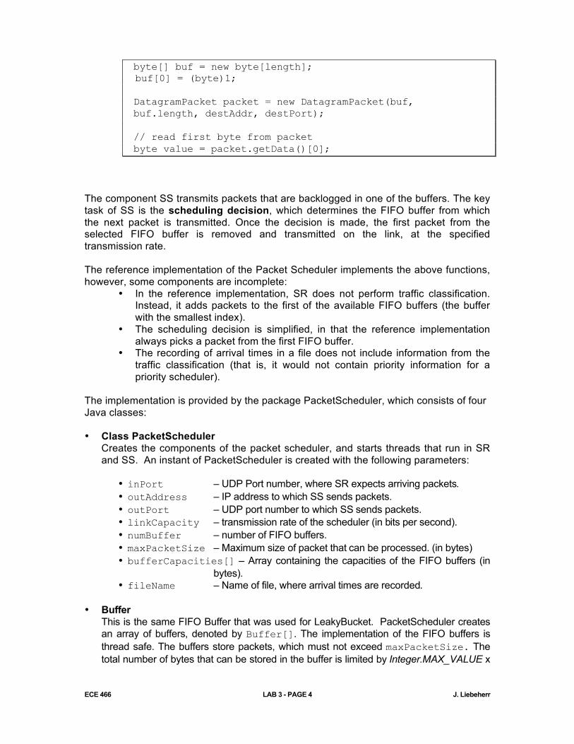
In essence, a PacketScheduler object receives packets from one or more traffic generators (TG), and forwards packet to a single traffic sink (TS). A PacketScheduler object has three components: a scheduler receiver (SR), a scheduler Sender (SS), and one ore more FIFO Buffers. The Scheduler Receiver SR processes incoming packets sent by the traffic generator(s), and adds the packet to one of the FIFO buffers. The scheduler inspects the first byte of each arriving packet to perform a traffic classification, which determines the FIFO buffer to which the packet must be added. Important: Traffic classification assumes that the traffic generator sets the first byte of the packet to the correct value. We refer to this process as traffic tagging. Therefore, previously used traffic generators must be modified so that they include traffic tagging. For example, for a priority scheduler, the traffic generators must tag each packet as either “High” or “Low” priority. When SR reads the tag, it can classify each packet as “High” or “Low” priority, and add the packet to the appropriate FIFO buffer. The following code segment shows an example of setting and reading the first byte of data from a packet.

// set first byte to 1 and create packet


byte[] buf = new byte[length]; buf[0] = (byte)1; DatagramPacket packet = new DatagramPacket(buf, buf.length, destAddr, destPort); // read first byte from packet byte value = packet.getData()[0];

The component SS transmits packets that are backlogged in one of the buffers. The key task of SS is the scheduling decision, which determines the FIFO buffer from which the next packet is transmitted. Once the decision is made, the first packet from the selected FIFO buffer is removed and transmitted on the link, at the specified transmission rate. The reference implementation of the Packet Scheduler implements the above functions, however, some components are incomplete:

• In the reference implementation, SR does not perform traffic classification. Instead, it adds packets to the first of the available FIFO buffers (the buffer with the smallest index).

• The scheduling decision is simplified, in that the reference implementation always picks a packet from the first FIFO buffer.

• The recording of arrival times in a file does not include information from the traffic classification (that is, it would not contain priority information for a priority scheduler).

The implementation is provided by the package PacketScheduler, which consists of four Java classes: • Class PacketScheduler

Creates the components of the packet scheduler, and starts threads that run in SR and SS. An instant of PacketScheduler is created with the following parameters:

• inPort – UDP Port number, where SR expects arriving packets. • outAddress – IP address to which SS sends packets. • outPort – UDP port number to which SS sends packets. • linkCapacity – transmission rate of the scheduler (in bits per second). • numBuffer – number of FIFO buffers. • maxPacketSize – Maximum size of packet that can be processed. (in bytes) • bufferCapacities[] – Array containing the capacities of the FIFO buffers (in

bytes). • fileName – Name of file, where arrival times are recorded.

• Buffer

This is the same FIFO Buffer that was used for LeakyBucket. PacketScheduler creates an array of buffers, denoted by Buffer[]. The implementation of the FIFO buffers is thread safe. The buffers store packets, which must not exceed maxPacketSize. The total number of bytes that can be stored in the buffer is limited by Integer.MAX_VALUE x


maxPacketSize. The capacity of Buffer[i] is given by bufferCapacity[i], specified in bytes. Each buffer has methods for adding packets to the tail of the buffer and removing packets from the head of the buffer, peeking at the first packet (without removing it), and querying the currently occupied buffer size (in terms of packets or bytes). When adding a newly arriving packet would exceed bufferCapacity[i], the packet is dropped.

• SchedulerReceiver (SR) Waits on a specified UDP port for incoming packets. When a packet arrives, the packet is first classified by inspecting the first byte of the packet. The content of the byte is mapped to an index of the FIFO buffer. The mapping depends on the type of scheduler used. Once classified, SR records the arrival time, size, buffer backlog of the queue, to a file. Then the packet is added to Buffer[index]:

Traffic classification: class = {content of first byte}; {Map class to index of the buffer array}; add packet to Buffer[index];

If a packet cannot be added to the buffer, e.g., because the buffer is full, the packet is dropped and an error message displayed.

• SchedulerSender (SS) SchedulerSender (SS) is responsible for selecting the buffer from which the next packet transmission occurs. This is referred to as the scheduling decision. The scheduling decision is dependent on the type of scheduling algorithm. The scheduler removes the first packet from the selected buffer and transmits the packet to the specified address (IP address and UDP port). The time to transmit a packet with size L bits is computed to be L/linkCapacity. If the actual transmission time is shorter than the computed transmission time, SS will sleep for the remaining time. The procedure for transmission is as follows:

If (at_least_one_buffer_is_not_empty) determine buffer from which packet is transmitted; remove first packet from selected buffer; determine computed transmission time of packet; transmit packet; sleep until the end of computed transmission time; else wait for packet to arrive to any buffer; // buffers wakes up SS when a packet arrives

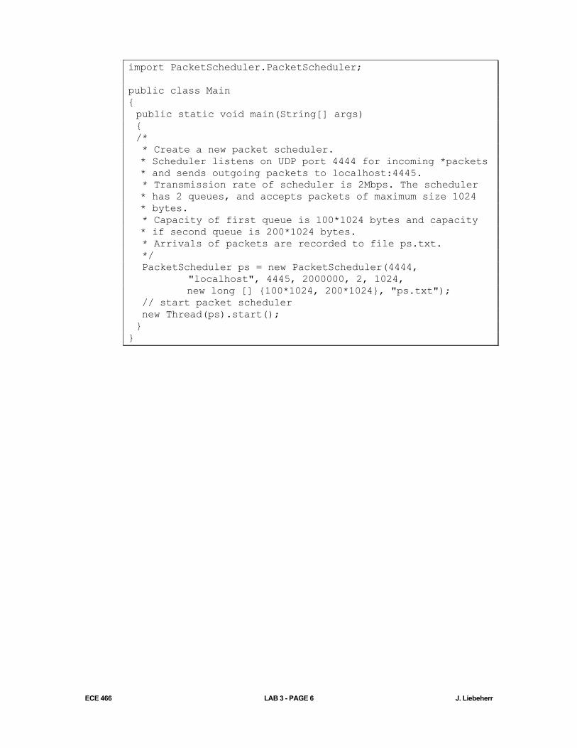
Note: In the reference implementation, the scheduling decision of SS only inspects the first buffer (Buffer[0]). The following code segment shows how you start PacketScheduler of the reference implementation in a process. The implementation assumes that the class PacketScheduler is in a subdirectory with name “PacketScheduler”:


import PacketScheduler.PacketScheduler; public class Main { public static void main(String[] args) { /* * Create a new packet scheduler. * Scheduler listens on UDP port 4444 for incoming *packets * and sends outgoing packets to localhost:4445. * Transmission rate of scheduler is 2Mbps. The scheduler * has 2 queues, and accepts packets of maximum size 1024 * bytes. * Capacity of first queue is 100*1024 bytes and capacity * if second queue is 200*1024 bytes. * Arrivals of packets are recorded to file ps.txt. */ PacketScheduler ps = new PacketScheduler(4444, "localhost", 4445, 2000000, 2, 1024, new long [] {100*1024, 200*1024}, "ps.txt"); // start packet scheduler new Thread(ps).start(); } }


Part 1. FIFO Scheduling

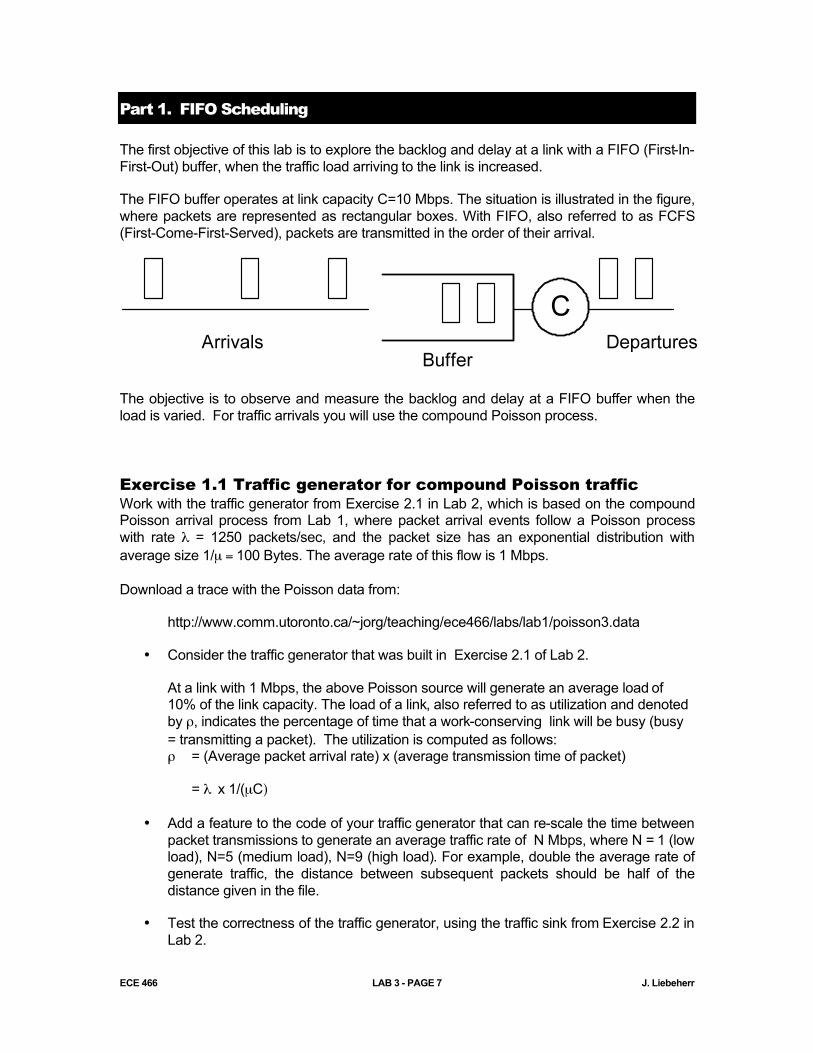
The first objective of this lab is to explore the backlog and delay at a link with a FIFO (First-In-First-Out) buffer, when the traffic load arriving to the link is increased.

The FIFO buffer operates at link capacity C=10 Mbps. The situation is illustrated in the figure, where packets are represented as rectangular boxes. With FIFO, also referred to as FCFS (First-Come-First-Served), packets are transmitted in the order of their arrival.

The objective is to observe and measure the backlog and delay at a FIFO buffer when the load is varied. For traffic arrivals you will use the compound Poisson process.

Exercise 1.1 Traffic generator for compound Poisson traffic Work with the traffic generator from Exercise 2.1 in Lab 2, which is based on the compound Poisson arrival process from Lab 1, where packet arrival events follow a Poisson process with rate λ = 1250 packets/sec, and the packet size has an exponential distribution with average size 1/µ = 100 Bytes. The average rate of this flow is 1 Mbps.

Download a trace with the Poisson data from:

http://www.comm.utoronto.ca/~jorg/teaching/ece466/labs/lab1/poisson3.data

• Consider the traffic generator that was built in Exercise 2.1 of Lab 2.

At a link with 1 Mbps, the above Poisson source will generate an average load of 10% of the link capacity. The load of a link, also referred to as utilization and denoted by ρ, indicates the percentage of time that a work-conserving link will be busy (busy = transmitting a packet). The utilization is computed as follows: ρ = (Average packet arrival rate) x (average transmission time of packet)

= λ x 1/(µC)

• Add a feature to the code of your traffic generator that can re-scale the time between packet transmissions to generate an average traffic rate of N Mbps, where N = 1 (low load), N=5 (medium load), N=9 (high load). For example, double the average rate of generate traffic, the distance between subsequent packets should be half of the distance given in the file.

• Test the correctness of the traffic generator, using the traffic sink from Exercise 2.2 in Lab 2.


Exercise 1.2 Implement a FIFO Scheduler Use the reference implementation of PacketScheduler to build a FIFO scheduler. The FIFO scheduler transmits packets in the order of their arrivals.

• Set the maximum size of the buffer in the FIFO scheduler to 100 kB. If the available buffer size is too small for an arriving packet, the packet is discarded (and a message is displayed.)

• Set the capacity of the link to 10 Mbps.

Note:

• With FIFO the scheduler only needs a single FIFO buffer.

• There is no need for traffic tagging (by the traffic generator) or traffic classification (by PacketReceiver).

Exercise 1.3 Observing a FIFO Scheduler at different loads Use the traffic generator to evaluate the FIFO scheduler with compound Poisson traffic at different loads.

• Use the added feature in the traffic generator from Exercise 1.1 and run the re-scaled Poisson trace file with an average rate of N Mbps, where N = 1 (low load), N=5 (medium load), N=9 (high load).

• For each value of N:

o Compute the backlog and waiting time for each packet processed by the packet scheduler. Note: The backlog can be determined when a packet arrives. Determining the waiting time requires that you know the arrival time and the departure time of a packet.

o Keep track of arriving packets that are discarded.

o Present plots that show the backlog, waiting time, and number of discarded packets, as a function of time.

• Designate ranges of N, where the FIFO scheduler is in a regime of low load and high load. Justify your choice.

Exercise 1.4 (Optional, 5% extra credit) Unfairness in FIFO A limitation of FIFO is that it cannot distinguish different traffic sources. Suppose that there are many low-bandwidth sources and a single traffic source that sends data at a very high rate. If the high-bandwidth source causes an overload at the link, then all traffic sources will experience packet losses due to buffer overflows. From the perspective of a low-bandwidth


source, this seems unfair. (The low-bandwidth source would like to see that packet losses experienced at the buffer are proportional to the traffic rate of a source).

The following experiment tries to exhibit the unfairness issues of FIFO for two traffic sources.

• There are two traffic sources, which are each re-scaled compound Poisson sources as in Exercise 1.1:

o Source 1 sends at an average rate of N1 Mbps.

o Source 2 sends at an average rate of N2 Mbps.

• Both sources send traffic into a FIFO scheduler (with rate C=1 Mbps) and 100 kB of buffer.

o Run a series of experiments where the load of the two sources is set to (N1, N2) with N1 = 5 and N2 = 1, 5, 10.

o Record the average throughput (output rate) of each traffic source (Note: You must be able to keep track whether a packet transmission is due to Source 1 or Source 2).

o Prepare a table that shows the average throughput values and interpret the result.

o Is it possible to write a formula that predicts the throughput as a function of the arrival rate?

Lab Report:

Provide the plots and a discussion of the plots. Also include answers to the questions.


Part 2. Priority Scheduling

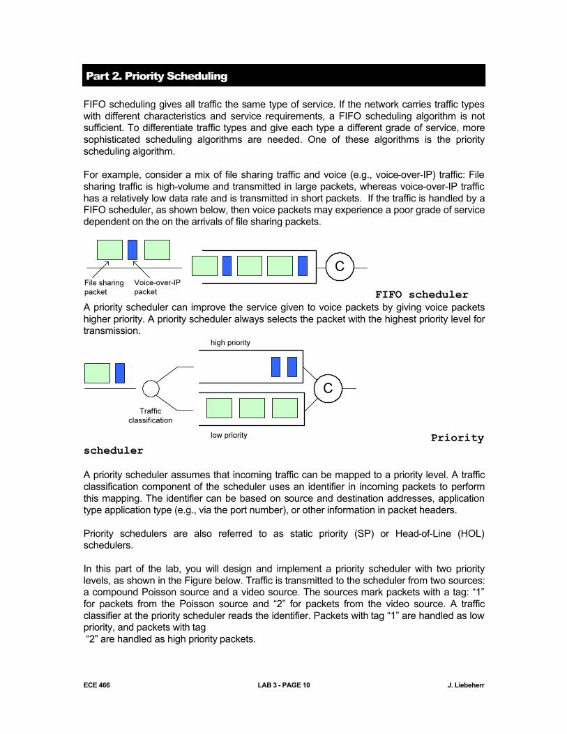
FIFO scheduling gives all traffic the same type of service. If the network carries traffic types with different characteristics and service requirements, a FIFO scheduling algorithm is not sufficient. To differentiate traffic types and give each type a different grade of service, more sophisticated scheduling algorithms are needed. One of these algorithms is the priority scheduling algorithm. For example, consider a mix of file sharing traffic and voice (e.g., voice-over-IP) traffic: File sharing traffic is high-volume and transmitted in large packets, whereas voice-over-IP traffic has a relatively low data rate and is transmitted in short packets. If the traffic is handled by a FIFO scheduler, as shown below, then voice packets may experience a poor grade of service dependent on the on the arrivals of file sharing packets.

FIFO scheduler A priority scheduler can improve the service given to voice packets by giving voice packets higher priority. A priority scheduler always selects the packet with the highest priority level for transmission.

Priority scheduler A priority scheduler assumes that incoming traffic can be mapped to a priority level. A traffic classification component of the scheduler uses an identifier in incoming packets to perform this mapping. The identifier can be based on source and destination addresses, application type application type (e.g., via the port number), or other information in packet headers. Priority schedulers are also referred to as static priority (SP) or Head-of-Line (HOL) schedulers. In this part of the lab, you will design and implement a priority scheduler with two priority levels, as shown in the Figure below. Traffic is transmitted to the scheduler from two sources: a compound Poisson source and a video source. The sources mark packets with a tag: “1” for packets from the Poisson source and “2” for packets from the video source. A traffic classifier at the priority scheduler reads the identifier. Packets with tag “1” are handled as low priority, and packets with tag “2” are handled as high priority packets.


Exercise 2.1 Transmission of tagged packets Build a traffic generator as shown on the left hand side of the figure above. The requirements for the transmission of packets are as follows:

• Build a traffic generator for a video tracefile and for a Poisson tracefile. The transmissions of the video source and the Poisson source are performed by two distinct programs.

• The Poisson tracefile is the tracefile from Part 1.

• The transmission of the video source is from the video tracefile, used in previous labs: http://www.comm.utoronto.ca/~jorg/teaching/ece466/labs/lab1/movietrace.data

Note: The average rate of traffic from the video source is approx. 15 Mbps.

• A traffic generator for the video source can be build by re-using the code from Exercise 1.2 and Exercise 2.1 from Lab 2. As in Lab 2, the maximum amount of data that can be put into a single packet is 1480 bytes. Frames exceeding this length are divided and transmitted in multiple packets.

• The transmission of the Poisson source is determined by the Poisson traffic generator built in Exercise 1.1 of this lab (Lab 3). The traffic generator must be able to run the re-scaled Poisson trace file with an average rate of N Mbps, where N = 1 (low load), N=5 (medium load), N=9 (high load).


• Before a packet is transmitted it must be tagged with an identifier, which is located in the first byte of the payload. The identifier is the number 0x01 for packets from the Poisson source and 0x02 for the video source.

• Packets are transmitted to a remote UDP port. Both sources transmit UDP datagrams to the same destination port on the same host (e.g., port 4444). You may use a traffic sink as build for Exercise 2.2 of Lab 2 for testing the implementation.

Exercise 2.2 Packet classification and priority scheduling Build a traffic classification and scheduling component as shown on the right hand side of the above figure.

• The priority scheduler consists of two FIFO queues: one FIFO queue for high priority traffic and one FIFO queue for low priority traffic. Set the maximum buffer size of each FIFO queue to 100 kB.

• The priority scheduler always transmits a high-priority packet, if the high priority FIFO queue contains a packet. Low priority packets are selected for transmission only when there are no high priority packets.

• The transmission rate of the link is C=20 Mbps.

• The traffic classification component reads the first byte of the payload of an arriving packet and identifies the priority label.

• Once classified, packets are assigned to the priority queues. Video traffic (with label “2”) is assigned to the high priority queue and Poisson traffic (with label “1”) is assigned to the low priority queue.

• If a new packet arrives when the link is idle (i.e., no packet is in transmission and no packet is waiting in the FIFO queues) the arriving packet is immediately transmitted. Otherwise, the packet is enqueued in the corresponding FIFO queue.

• The priority scheduler is work-conserving: As long as there is a packet waiting, the scheduler must transmit a packet.

• Packet transmissions is non-preemptive: Once the transmission of a packet has started, the transmission cannot be interrupted. In particular, when a low priority packet is in transmission, an arriving high-priority packet must wait until the transmission is completed.

Test the implementation with the traffic generator from Exercise 2.1.

Exercise 2.3 Evaluation of the priority scheduler Evaluate the priority scheduler with the traffic generator Exercise 2.1 using the following transmission scenarios:

• The video source transmits according to the data in the tracefile (see Exercise 2.1).


• As in Exercise 1.1, the Poisson source should be scaled so that it transmits with an average rate of N Mbps, where N = 1 (low load), N=5 (medium load), N=9 (high load).

• For each value of N, determine the following values for both high priority (video) and low priority (Poisson) traffic:

o Compute the backlog and waiting time for each packet processed by the packet scheduler. Note: The backlog can be determined when a packet arrives. Determining the waiting time requires that you know the arrival time and the departure time of a packet.

o Keep track of arriving packets that are discarded.

o Present plots that show the backlog, waiting time, and number of discarded packets, as a function of time.

• Compare the outcome to Exercise 1.3.

Exercise 2.4 (Optional, 5% extra credit) Starvation in priority schedulers A limitation of SP scheduling is that it always gives preference to high-priority scheduling. If the load from high-priority traffic is very high, it may completely pre-empt low-priority traffic from the link. This is referred to as starvation.

The following experiment tries to exhibit the starvation of low priority traffic. The experiment is similar to the last exercise of Part 1.

• The link capacity should be set to C=10 Mbps.

• Consider the previously build priority scheduler with two priority classes.


o Source 1 transmits at an average rate of N1 Mbps.


o Traffic from Source 1 is labelled with identifier “1” (low priority) and Source 2 is labelled with “2” (high priority).

• Both sources send traffic to the priority scheduler (with rate C=10 Mbps) and 100 kB of buffer for each queue.

o Run a series of experiments where the load of the two sources is set to (N1, N2) with N1 = 5 and N2 = 1, 5, and 9.

o Record the average throughput (output rate) of each traffic source.


o Prepare a table that shows the average throughput of high and low priority traffic and interpret the result.

o Compare the outcome to Exercise 1.4.

Lab Report:



Part 3. Weighted Round Robin (WRR) Scheduler

Many scheduling algorithms attempt to achieve a notion of fairness by regulating the fraction of link bandwidth allocated to each traffic source. The objectives of a “fair scheduler” are as follows: If the link is not overloaded, a traffic source should be able to transmit all of its traffic. If the link is overloaded, each traffic source obtains the same rate guarantee, called the fair share, with the following rules: • If the traffic from a source is less than the fair share, it can transmit all its traffic; • If the traffic from a source exceeds the fair share, it can transmit at a rate equal to the fair

share. The fair share depends on the number of active sources and their traffic rate. Suppose we have set of sources where the arrival rate of Source i is ri, and a link with capacity C (bps). If

the arrival rate exceeds the capacity, i.e., , then the fair share is the number f that satisfies the equation:

As an example, suppose we have a link with capacity 10 Mbps, and the arrival rates of flows are r1=8 Mbps, r2= 6 Mbps, and r3= 2 Mbps, then the fair share is f = 4 Mbps, resulting in an allocated rate is 4 Mbps for Source 1, 4 Mbps for Source 2, and 2 Mbps for Source 3.

Since different sources have different resource requirements, it is often desirable to associate a weight (wi) with each source, and allocate bandwidth proportionally to the weights. In other words, a source that has a weight twice as large of second source should be able to obtain twice the bandwidth of the second source. With these weights, the fair share f at an

overloaded link, i.e., is obtained by solving . For example, using the previous example, and assigning weights w1=3, w2=w3=1, the allocated rates are 6, 2, and 2 Mbps for the three sources.

A scheduling algorithm that realizes this scheme without weights is called Processor Sharing (PS) and with weights Generalized Processor Sharing (GPS). Both PS and GPS are idealized algorithms, since they treat traffic as a fluid. Realizing fairness in a packet network turns out to be quite hard, since packet sizes have different sizes (50 – 1500 bytes) and packet transmissions cannot be interrupted. Many commercial IP routers and Ethernet


switches (not the cheap ones!) implement scheduling algorithms that approximate the GPS scheduling algorithm. A widely used (and easy to implement) scheduling algorithm that approximates GPA is the Weighted Round Robin (WRR) scheduler. The objective of this part of the lab is implementing and evaluating a WRR scheduling algorithm.

A WRR scheduler, illustrated in the figure above, operates as follows: • The scheduler has multiple FIFO queues. A traffic classification unit assigns an incoming

packet to one of the FIFO queues.

• The WRR scheduler operates in “rounds”. In each round the scheduler visits each queue in a round-robin (sic!) fashion, starting with Queue 1. During each visit of a queue one or more packets may be serviced.

• The WRR assumes that one can estimate (or know) the average packet size of the arrivals to Queue i, denoted by Li.

• The WRR calculates the number of packets to be served in each round:

o For each Queue i: xi = wi / Li

o x = mini { xi }

o For each Queue i: packets_per_roundi = xi / x

• Once all packets of a round are transmitted or if no more packets are left, the scheduler visits the next queue.


Exercise 3.1 Build a WRR scheduler Build a WRR scheduler as described above, that supports at least three queues. The WRR will serve Poisson traffic sources as used in Parts 1 and 2 of this lab.

• A WRR scheduler requires one FIFO buffer (queue) for each flow.

• There are three traffic generators that each transmit re-scaled Poisson traffic as done in Exercise 1.1. Each Poisson source is re-scaled so that it transmits with an average rate of N Mbps, where N = 1 (low load), N=5 (medium load), N=9 (high load).

• Each transmitted packet is labelled with “1”, “2” or “3” as done in Part 2 of this lab. The label is one byte long. The traffic classification component reads the first byte of the payload of an arriving packet, and adds the packet to the queue (Packets with label “1” are associated with Queue 1, etc.). If no packet is in transmission or in the queue, and arriving packet is transmitted immediately.

• The transmission rate of the link is C=10 Mbps. The maximum buffer size of each queue is 100 kB. An arrival that cannot be stored in the queue is discarded.

Once the implementation is completed and tested, move on to the evaluation.

Exercise 3.2 Evaluation of a WRR scheduler: Equal weights Evaluate the WRR scheduler with three Poisson sources.

o The weight N of the traffic generators are set to N=8 in for the first source, N=6 for the second source and N=2 for the third source, resulting in traffic arrival rates of 8 Mbps, 6 Mbps, and 2 Mbps.

o Set the weights of the queues to w1=w2=w3=1.

Note: Compare this scenario to the first figure of Part 3. The average load on the link is 1.5 Mbps, i.e., the link is overloaded. We expect that the bandwidth at the link is shared among the sources at a ratio of 4:4:2.

• Prepare plots that show the number of packet transmissions and the number of transmitted bytes from a particular source (y-axis) as a function of time (x-axis). Provide one plot for each source.


Select a reasonable time scale for the x-axis, e.g., a time scale of 10 ms per data point.

• Compare the plots with the theoretically expected values of a PS scheduler.

Exercise 3.3 Evaluation of a WRR scheduler: Different weights This exercise re-creates a transmission scenario as in the second figure of Part 3.

o Evaluate the WRR scheduler with three Poisson sources. As before, the weight N of the traffic generators is set to N=8 in for the first source, N=6 for the second source and N=2 for the third source.

o Set the weights of the queues to w1=3 and w2=w3=1.

Note: Compare this scenario to the second figure of Part 3. We expect that the bandwidth at the link is shared among the sources at a ratio of 6:2:2.

• Prepare plots that show the number of packet transmissions and the number of transmitted bytes from a particular source (y-axis) as a function of time (x-axis). Provide one plot for each source.

• Compare the plots with the theoretically expected values of a GPS scheduler.

Exercise 3.4 (Optional, 5% extra credit) No Unfairness and no Starvation in WRR A limitation of SP scheduling is that it always gives preference to high-priority scheduling. If the load from high-priority traffic is very high, it may completely pre-empt low-priority traffic from the link. This is referred to as starvation.

The following experiment tries to show that WRR does not suffer from the problems of FIFO (unfair) and SP (starvation). The experiment retraces the steps of Exercises 1.4 and 2.4.

• Consider the WRR scheduler from above with rate C=10 Mbps and 100 kB of buffer for each queue.




o Traffic from Source 1 is labelled with identifier “1” (low priority) and Source 2 is labelled with “2” (high priority).

o Both sources are assigned the same weight at the WRR scheduler (w1=w2=1).

• Run a series of experiments where the load of the two sources is set to (N1, N2) with N1 = 5 and N2 = 5, 9, 15.


o Record the average throughput (output rate) of each traffic source.

o Prepare a table that shows the average throughput of the two sources and interpret the result.

o Compare the outcome to Exercises 1.4 and 2.4.

Lab Report:



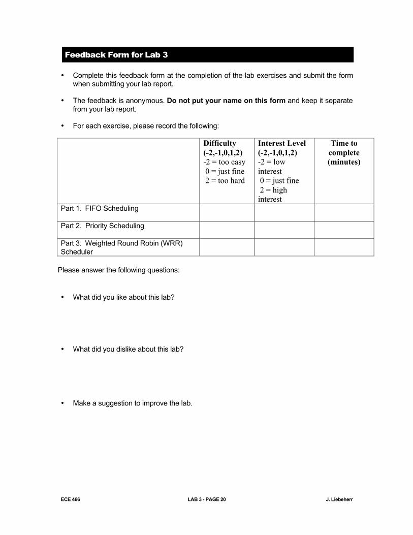
Feedback Form for Lab 3 • Complete this feedback form at the completion of the lab exercises and submit the form

when submitting your lab report.

• The feedback is anonymous. Do not put your name on this form and keep it separate from your lab report.

• For each exercise, please record the following:

Difficulty (-2,-1,0,1,2) -2 = too easy 0 = just fine 2 = too hard

Interest Level (-2,-1,0,1,2) -2 = low interest 0 = just fine 2 = high interest

Time to complete (minutes)

Part 1. FIFO Scheduling

Part 2. Priority Scheduling

Part 3. Weighted Round Robin (WRR) Scheduler

Please answer the following questions: • What did you like about this lab?

• What did you dislike about this lab?

• Make a suggestion to improve the lab.

packet schedulingjorg/teaching/ece466/labs/lab3_v3c.pdfweighted round robin ... you will implement...

Documents