package ‘timsac’ - the comprehensive r archive network · pdf filepackage...

Package ‘timsac’March 6, 2018

Version 1.3.6

Title Time Series Analysis and Control Package

Author The Institute of Statistical Mathematics

Maintainer Masami Saga <[email protected]>

Depends R (>= 3.0.0)

Imports graphics, grDevices, stats

Description Functions for statistical analysis, prediction and control of timeseries based mainly on Akaike and Nakagawa (1988) <ISBN 978-90-277-2786-2>.

License GPL (>= 2)

MailingList Please send bug reports to [email protected].

NeedsCompilation yes

Repository CRAN

Date/Publication 2018-03-06 15:54:00 UTC

R topics documented:timsac-package . . . . . . . . . . . . . . . . . . . . . . . . . . . . . . . . . . . . . . . 2Airpollution . . . . . . . . . . . . . . . . . . . . . . . . . . . . . . . . . . . . . . . . . 3Amerikamaru . . . . . . . . . . . . . . . . . . . . . . . . . . . . . . . . . . . . . . . . 4armafit . . . . . . . . . . . . . . . . . . . . . . . . . . . . . . . . . . . . . . . . . . . . 4auspec . . . . . . . . . . . . . . . . . . . . . . . . . . . . . . . . . . . . . . . . . . . . 5autcor . . . . . . . . . . . . . . . . . . . . . . . . . . . . . . . . . . . . . . . . . . . . 6autoarmafit . . . . . . . . . . . . . . . . . . . . . . . . . . . . . . . . . . . . . . . . . 7baysea . . . . . . . . . . . . . . . . . . . . . . . . . . . . . . . . . . . . . . . . . . . . 8bispec . . . . . . . . . . . . . . . . . . . . . . . . . . . . . . . . . . . . . . . . . . . . 10bispecData . . . . . . . . . . . . . . . . . . . . . . . . . . . . . . . . . . . . . . . . . . 11blocar . . . . . . . . . . . . . . . . . . . . . . . . . . . . . . . . . . . . . . . . . . . . 12blomar . . . . . . . . . . . . . . . . . . . . . . . . . . . . . . . . . . . . . . . . . . . . 13Blsallfood . . . . . . . . . . . . . . . . . . . . . . . . . . . . . . . . . . . . . . . . . . 14bsubst . . . . . . . . . . . . . . . . . . . . . . . . . . . . . . . . . . . . . . . . . . . . 15Canadianlynx . . . . . . . . . . . . . . . . . . . . . . . . . . . . . . . . . . . . . . . . 17canarm . . . . . . . . . . . . . . . . . . . . . . . . . . . . . . . . . . . . . . . . . . . . 18

1

2 timsac-package

canoca . . . . . . . . . . . . . . . . . . . . . . . . . . . . . . . . . . . . . . . . . . . . 19covgen . . . . . . . . . . . . . . . . . . . . . . . . . . . . . . . . . . . . . . . . . . . . 21decomp . . . . . . . . . . . . . . . . . . . . . . . . . . . . . . . . . . . . . . . . . . . 21exsar . . . . . . . . . . . . . . . . . . . . . . . . . . . . . . . . . . . . . . . . . . . . . 24fftcor . . . . . . . . . . . . . . . . . . . . . . . . . . . . . . . . . . . . . . . . . . . . . 25fpeaut . . . . . . . . . . . . . . . . . . . . . . . . . . . . . . . . . . . . . . . . . . . . 26fpec . . . . . . . . . . . . . . . . . . . . . . . . . . . . . . . . . . . . . . . . . . . . . 27LaborData . . . . . . . . . . . . . . . . . . . . . . . . . . . . . . . . . . . . . . . . . . 28locarData . . . . . . . . . . . . . . . . . . . . . . . . . . . . . . . . . . . . . . . . . . 29markov . . . . . . . . . . . . . . . . . . . . . . . . . . . . . . . . . . . . . . . . . . . 29mfilter . . . . . . . . . . . . . . . . . . . . . . . . . . . . . . . . . . . . . . . . . . . . 31mlocar . . . . . . . . . . . . . . . . . . . . . . . . . . . . . . . . . . . . . . . . . . . . 32mlomar . . . . . . . . . . . . . . . . . . . . . . . . . . . . . . . . . . . . . . . . . . . 34mulbar . . . . . . . . . . . . . . . . . . . . . . . . . . . . . . . . . . . . . . . . . . . . 35mulcor . . . . . . . . . . . . . . . . . . . . . . . . . . . . . . . . . . . . . . . . . . . . 37mulfrf . . . . . . . . . . . . . . . . . . . . . . . . . . . . . . . . . . . . . . . . . . . . 38mulmar . . . . . . . . . . . . . . . . . . . . . . . . . . . . . . . . . . . . . . . . . . . 39mulnos . . . . . . . . . . . . . . . . . . . . . . . . . . . . . . . . . . . . . . . . . . . . 41mulrsp . . . . . . . . . . . . . . . . . . . . . . . . . . . . . . . . . . . . . . . . . . . . 42mulspe . . . . . . . . . . . . . . . . . . . . . . . . . . . . . . . . . . . . . . . . . . . . 43nonst . . . . . . . . . . . . . . . . . . . . . . . . . . . . . . . . . . . . . . . . . . . . . 45nonstData . . . . . . . . . . . . . . . . . . . . . . . . . . . . . . . . . . . . . . . . . . 46optdes . . . . . . . . . . . . . . . . . . . . . . . . . . . . . . . . . . . . . . . . . . . . 46optsim . . . . . . . . . . . . . . . . . . . . . . . . . . . . . . . . . . . . . . . . . . . . 47perars . . . . . . . . . . . . . . . . . . . . . . . . . . . . . . . . . . . . . . . . . . . . 49Powerplant . . . . . . . . . . . . . . . . . . . . . . . . . . . . . . . . . . . . . . . . . 50prdctr . . . . . . . . . . . . . . . . . . . . . . . . . . . . . . . . . . . . . . . . . . . . 51raspec . . . . . . . . . . . . . . . . . . . . . . . . . . . . . . . . . . . . . . . . . . . . 52sglfre . . . . . . . . . . . . . . . . . . . . . . . . . . . . . . . . . . . . . . . . . . . . 53simcon . . . . . . . . . . . . . . . . . . . . . . . . . . . . . . . . . . . . . . . . . . . . 54thirmo . . . . . . . . . . . . . . . . . . . . . . . . . . . . . . . . . . . . . . . . . . . . 56unibar . . . . . . . . . . . . . . . . . . . . . . . . . . . . . . . . . . . . . . . . . . . . 57unimar . . . . . . . . . . . . . . . . . . . . . . . . . . . . . . . . . . . . . . . . . . . . 59wnoise . . . . . . . . . . . . . . . . . . . . . . . . . . . . . . . . . . . . . . . . . . . . 60xsarma . . . . . . . . . . . . . . . . . . . . . . . . . . . . . . . . . . . . . . . . . . . . 61

Index 63

timsac-package Time Series Analysis and Control Program Package

Description

R functions for statistical analysis and control of time series.

Airpollution 3

Details

This package provides functions for statistical analysis, prediction and control of time series. Theoriginal TIMSAC (TIMe Series Analysis and Control) or TIMSAC-72 was published in Akaike andNakagawa (1972). After that, TIMSAC-74, TIMSAC-78 and TIMSAC-84 were published as theTIMSAC series in Computer Science Monograph.

For overview of models and information criteria for model selection, see ../doc/timsac-guide_e.pdf or ../doc/timsac-guide_j.pdf (in Japanese).

References

H.Akaike, E.Arahata and T.Ozaki (1975) Computer Science Monograph, No.5, Timsac74, A TimeSeries Analysis and Control Program Package (1). The Institute of Statistical Mathematics.


H.Akaike, G.Kitagawa, E.Arahata and F.Tada (1979) Computer Science Monograph, No.11, Tim-sac78. The Institute of Statistical Mathematics.

H.Akaike, T.Ozaki, M.Ishiguro, Y.Ogata, G.Kitagawa, Y-H.Tamura, E.Arahata, K.Katsura andY.Tamura (1985) Computer Science Monograph, No.22, Timsac84 Part 1. The Institute of Sta-tistical Mathematics.

H.Akaike and T.Nakagawa (1988) Statistical Analysis and Control of Dynamic Systems. KluwerAcademic publishers.

Airpollution Airpollution Data

Description

An airpollution data for testing perars.

Usage

data(Airpollution)

Format

A time series of 372 observations.

Source


../doc/timsac-guide_e.pdf

../doc/timsac-guide_e.pdf

../doc/timsac-guide_j.pdf

4 armafit

Amerikamaru Amerikamaru Data

Description

A multivariate non-stationary data for testing blomar.

Usage

data(Amerikamaru)

Format

A 2-dimensional array with 896 observations on 2 variables.

[, 1] rudder[, 2] yawing

Source


armafit ARMA Model Fitting

Description

Fit an ARMA model with specified order by using DAVIDON’s algorithm.

Usage

armafit(y, model.order)

Arguments

y a univariate time series.model.order a numerical vector of the form c(ar, ma) which gives the order to be fitted suc-

cessively.

Details

The maximum likelihood estimates of the coefficients of a scalar ARMA model

y(t)− a(1)y(t− 1)− ...− a(p)y(t− p) = u(t)− b(1)u(t− 1)− ...− b(q)u(t− q)

of a time series y(t) are obtained by using DAVIDON’s algorithm. Pure autoregression is notallowed.

auspec 5

Value

arcoef maximum likelihood estimates of AR coefficients.macoef maximum likelihood estimates of MA coefficients.arstd standard deviation (AR).mastd standard deviation (MA).v innovation variance.aic AIC.grad final gradient.

References


Examples

# "arima.sim" is a function in "stats".# Note that the sign of MA coefficient is opposite from that in "timsac".y <- arima.sim(list(order=c(2,0,1), ar=c(0.64,-0.8), ma=-0.5), n = 1000)z <- armafit(y, model.order = c(2,1))z$arcoefz$macoef

auspec Power Spectrum

Description

Compute power spectrum estimates for two trigonometric windows of Blackman-Tukey type byGoertzel method.

Usage

auspec(y, lag = NULL, window = "Akaike", log = FALSE, plot = TRUE)

Arguments

y a univariate time series.lag maximum lag. Default is 2

√n, where n is the length of time series y.

window character string giving the definition of smoothing window. Allowed strings are"Akaike" (default) or "Hanning".

log logical. If TRUE, the spectrum spec is plotted as log(spec).plot logical. If TRUE (default), the spectrum spec is plotted.

Details

6 autcor

Hanning Window : a1(0)=0.5, a1(1)=a1(-1)=0.25, a1(2)=a1(-2)=0Akaike Window : a2(0)=0.625, a2(1)=a2(-1)=0.25, a2(2)=a2(-2)=-0.0625

Value

spec spectrum smoothing by ’window’

stat test statistics.

References


Examples

y <- arima.sim(list(order=c(2,0,0), ar=c(0.64,-0.8)), n = 200)auspec(y, log = TRUE)

autcor Autocorrelation

Description

Estimate autocovariances and autocorrelations.

Usage

autcor(y, lag = NULL, plot = TRUE, lag_axis = TRUE)

Arguments

y a univariate time series.

lag maximum lag. Default is 2√n, where n is the length of the time series y.

plot logical. If TRUE (default), autocorrelations are plotted.

lag_axis logical. If TRUE (default) with plot = TRUE, x-axis is drawn.

Value

acov autocovariances.

acor autocorrelations (normalized covariances).

mean mean of y.

autoarmafit 7

References


Examples

# Example 1 for the normal distributiony <- rnorm(200)autcor(y, lag_axis = FALSE)

# Example 2 for the ARIMA modely <- arima.sim(list(order=c(2,0,0), ar=c(0.64,-0.8)), n = 200)autcor(y, lag = 20)

autoarmafit Automatic ARMA Model Fitting

Description

Provide an automatic ARMA model fitting procedure. Models with various orders are fitted and thebest choice is determined with the aid of the statistics AIC.

Usage

autoarmafit(y, max.order = NULL)

Arguments

y a univariate time series.max.order upper limit of AR order and MA order. Default is 2

√n, where n is the length of

the time series y.

Details

The maximum likelihood estimates of the coefficients of a scalar ARMA model

y(t)− a(1)y(t− 1)− ...− a(p)y(t− p) = u(t)− b(1)u(t− 1)− ...− b(q)u(t− q)

of a time series y(t) are obtained by using DAVIDON’s variance algorithm. Where p is AR order,q is MA order and u(t) is a zero mean white noise. Pure autoregression is not allowed.

Value

best.model the best choice of ARMA coefficients.model a list with components arcoef (Maximum likelihood estimates of AR coef-

ficients), macoef (Maximum likelihood estimates of MA coefficients), arstd(AR standard deviation), mastd (MA standard deviation), v (Innovation vari-ance), aic (AIC = n log(det(v)) + 2(p+ q)) and grad (Final gradient) in AICincreasing order.

8 baysea

References


Examples

# "arima.sim" is a function in "stats".# Note that the sign of MA coefficient is opposite from that in "timsac".y <- arima.sim(list(order=c(2,0,1),ar=c(0.64,-0.8),ma=-0.5), n = 1000)autoarmafit(y)

baysea Bayesian Seasonal Adjustment Procedure

Description

Decompose a nonstationary time series into several possible components.

Usage

baysea(y, period = 12, span = 4, shift = 1, forecast = 0, trend.order = 2,seasonal.order = 1, year = 0, month = 1, out = 0, rigid = 1,zersum = 1, delta = 7, alpha = 0.01, beta = 0.01, gamma = 0.1,spec = TRUE, plot = TRUE, separate.graphics = FALSE)

Arguments


period number of seasonals within a period.

span number of periods to be processed at one time.

shift number of periods to be shifted to define the new span of data.

forecast length of forecast at the end of data.

trend.order order of differencing of trend.

seasonal.order order of differencing of seasonal. seasonal.order is smaller than or equal tospan.

year trading-day adjustment option.

= 0 : without trading day adjustment> 0 : with trading day adjustment

(the series is supposed to start at this year)

month number of the month in which the series starts. If year=0 this parameter isignored.

out outlier correction option.

baysea 9

0 : without outlier detection1 : with outlier detection by marginal probability2 : with outlier detection by model selection

rigid controls the rigidity of the seasonal component. more rigid seasonal with largerthan rigid.

zersum controls the sum of the seasonals within a period.

delta controls the leap year effect.

alpha controls prior variance of initial trend.

beta controls prior variance of initial seasonal.

gamma controls prior variance of initial sum of seasonal.

spec logical. If TRUE (default), estimate spectra of irregular and differenced adjusted.

plot logical. If TRUE (default), plot trend, adjust, smoothed, season and irregular.separate.graphics

logical. If TRUE, a graphic device is opened for each graphics display.

Details

This function realized a decomposition of time series y into the form

y(t) = T (t) + S(t) + I(t) + TDC(t) +OCF (t)

where T (t) is trend component, S(t) is seasonal component, I(t) is irregular, TDC(t) is tradingday factor and OCF (t) is outlier correction factor. For the purpose of comparison of models thecriterion ABIC is defined

ABIC = −2 log(maximum likelihood of the model).

Smaller value of ABIC represents better fit.

Value

outlier outlier correction factor.

trend trend.

season seasonal.

tday trading day component if year > 0.

irregular = y - trend - season - tday - outlier.

adjust = trend - irregular.

smoothed = trend + season + tday.

aveABIC averaged ABIC.

irregular.spec a list with components acov (autocovariances), acor (normalized covariances),mean, v (innovation variance), aic (AIC), parcor (partial autocorrelation) andrspec (rational spectrum) of irregular if spec = TRUE.

adjusted.spec a list with components acov, acor, mean, v, aic, parcor and rspec of differ-enced adjusted series if spec = TRUE.

10 bispec

differenced.trend

a list with components acov, acor, mean, v, aic and parcor of differenced trendseries if spec = TRUE.

differenced.season

a list with components acov, acor, mean, v, aic and parcor of differencedseasonal series if spec = TRUE.

References


Examples

data(LaborData)baysea(LaborData, forecast = 12)

bispec Bispectrum

Description

Compute bi-spectrum using the direct Fourier transform of sample third order moments.

Usage

bispec(y, lag = NULL, window = "Akaike", log = FALSE, plot = TRUE)

Arguments




log logical. If TRUE, the spectrum pspec is plotted as log(pspec).

plot logical. If TRUE (default), the spectrum pspec is plotted.

Details


bispecData 11

Value

pspec power spectrum smoothed by ’window’.

sig significance.

cohe coherence.

breal real part of bispectrum.

bimag imaginary part of bispectrum.

exval approximate expected value of coherence under Gaussian assumption.

References


Examples

data(bispecData)bispec(bispecData, lag = 30)

bispecData Univariate Test Data

Description

A univariate data for testing bispec and thirmo.

Usage

data(bispecData)

Format


Source

H.Akaike, E.Arahata and T.Ozaki (1976) Computer Science Monograph, No.6, Timsac74 A TimeSeries Analysis and Control Program Package (2). The Institute of Statistical Mathematics.

12 blocar

blocar Bayesian Method of Locally Stationary AR Model Fitting; Scalar Case

Description

Locally fit autoregressive models to non-stationary time series by a Bayesian procedure.

Usage

blocar(y, max.order = NULL, span, plot = TRUE)

Arguments


max.order upper limit of the order of AR model. Default is 2√n, where n is the length of

the time series y.

span length of basic local span.

plot logical. If TRUE (default), spectrums pspec are plotted.

Details

The basic AR model of scalar time series y(t)(t = 1, . . . , n) is given by

y(t) = a(1)y(t− 1) + a(2)y(t− 2) + . . .+ a(p)y(t− p) + u(t),

where p is order of the model and u(t) is Gaussian white noise with mean 0 and variance v. At eachstage of modeling of locally AR model, a two-step Bayesian procedure is applied

1. Averaging of the models with different orders fitted to the newly obtained data.2. Averaging of the models fitted to the present and preceding spans.

AIC of the model fitted to the new span is defined by

AIC = ns log(sd) + 2k,

where ns is the length of new data, sd is innovation variance and k is the equivalent number ofparameters, defined as the sum of squares of the Bayesian weights. AIC of the model fitted to thepreceding spans are defined by

AIC(j + 1) = ns log(sd(j)) + 2,

where sd(j) is the prediction error variance by the model fitted to j periods former span.

Value

var variance.

aic AIC.

blomar 13

bweight Bayesian weight.

pacoef partial autocorrelation.

arcoef coefficients ( average by the Bayesian weights ).

v innovation variance.

init initial point of the data fitted to the current model.

end end point of the data fitted to the current model.

pspec power spectrum.

References

G.Kitagawa and H.Akaike (1978) A Procedure for The Modeling of Non-Stationary Time Series.Ann. Inst. Statist. Math., 30, B, 351–363.

H.Akaike (1978) A Bayesian Extension of the Minimum AIC Procedure of Autoregressive ModelFitting. Research Memo. NO.126. The Institute of The Statistical Mathematics.


Examples

data(locarData)z <- blocar(locarData, max.order = 10, span = 300)z$arcoef

blomar Bayesian Method of Locally Stationary Multivariate AR Model Fitting

Description

Locally fit multivariate autoregressive models to non-stationary time series by a Bayesian proce-dure.

Usage

blomar(y, max.order = NULL, span)

Arguments

y A multivariate time series.

max.order upper limit of the order of AR model, less than or equal to n/2d where n is thelength and d is the dimension of the time series y. Default is min(2

√n, n/2d).

span length of basic local span. Let m denote max.order, if n −m − 1 is less thanor equal to span or n−m− 1−span is less than 2md, span is n−m.

14 Blsallfood

Details

The basic AR model is given by

y(t) = A(1)y(t− 1) +A(2)y(t− 2) + . . .+A(p)y(t− p) + u(t),

where p is order of the AR model and u(t) is innovation variance v.

Value

mean mean.

var variance.

bweight Bayesian weight.

aic AIC with respect to the present data.

arcoef AR coefficients. arcoef[[m]][i,j,k] shows the value of i-th row, j-th col-umn, k-th order of m-th model.


eaic equivalent AIC of Bayesian model.

init start point of the data fitted to the current model.


References

G.Kitagawa and H.Akaike (1978) A Procedure for the Modeling of Non-stationary Time Series.Ann. Inst. Statist. Math., 30, B, 351–363.

H.Akaike (1978) A Bayesian Extension of The Minimum AIC Procedure of Autoregressive ModelFitting. Research Memo. NO.126. The institute of Statistical Mathematics.


Examples

data(Amerikamaru)blomar(Amerikamaru, max.order = 10, span = 300)

Blsallfood Blsallfood data

Description

A blsallfood data for testing decomp.

Usage

data(Blsallfood)

bsubst 15

Format


Source

H.Akaike, T.Ozaki, M.Ishiguro, Y.Ogata, G.Kitagawa, Y-H.Tamura, E.Arahata, K.Katsura andY.Tamura (1984) Computer Science Monographs, Timsac-84 Part 1. The Institute of StatisticalMathematics.

bsubst Bayesian Type All Subset Analysis

Description

Produce Bayesian estimates of time series models such as pure AR models, AR models with non-linear terms, AR models with polynomial type mean value functions, etc. The goodness of fit of amodel is checked by the analysis of several steps ahead prediction errors.

Usage

bsubst(y, mtype, lag = NULL, nreg, reg = NULL, term.lag = NULL, cstep = 5,plot = TRUE)

Arguments


mtype model type. Allowed values are

1 : autoregressive model,2 : polynomial type non-linear model (lag’s read in),3 : polynomial type non-linear model (lag’s automatically set),4 : AR-model with polynomial mean value function,

5,6,7 : originally defined but omitted here.

lag maximum time lag. Default is 2√n, where n is the length of the time series y.

nreg number of regressors.

reg specification of regressor (mtype = 2).i-th regressor is defined by z(n−L1(i))× z(n−L2(i))× z(n−L3(i)), whereL1(i) is reg(1,i), L2(i) is reg(2,i) and L3(i) is reg(3,i). 0-lag term z(n−0) is replaced by the constant 1.

term.lag maximum time lag specify the regressors (L1(i), L2(i), L3(i)) (i=1,. . . ,nreg)(mtype = 3).

term.lag[1] : maximum time lag of linear termterm.lag[2] : maximum time lag of squared termterm.lag[3] : maximum time lag of quadratic crosses term

16 bsubst

term.lag[4] : maximum time lag of cubic termterm.lag[5] : maximum time lag of cubic cross term.

cstep prediction errors checking (up to cstep-steps ahead) is requested. (mtype = 1,2, 3).

plot logical. If TRUE (default), daic, perr and peautcor are plotted.

Details

The AR model is given by ( mtype = 2 )

y(t) = a(1)y(t− 1) + ...+ a(p)y(t− p) + u(t).

The non-linear model is given by ( mtype = 2, 3 )

y(t) = a(1)z(t, 1) + a(2)z(t, 2) + ...+ a(p)z(t, p) + u(t).

Where p is AR order and u(t) is Gaussian white noise with mean 0 and variance v(p).

Value

ymean mean of y.

yvar variance of y.


aic AIC(m), (m=0, . . .nreg).

aicmin minimum AIC.

daic AIC(m)-aicmin (m=0, . . .nreg).

order.maice order of minimum AIC.

v.maice innovation variance attained at order.maice.

arcoef.maice AR coefficients attained at order.maice.

v.bay residual variance of Bayesian model.

aic.bay AIC of Bayesian model.

np.bay equivalent number of parameters.

arcoef.bay AR coefficients of Bayesian model.

ind.c index of parcor2 in order of increasing magnitude.

parcor2 square of partial correlations (normalized by multiplying N).

damp binomial type damper.

bweight final Bayesian weights of partial correlations.

parcor.bay partial correlations of the Bayesian model.

eicmin minimum EIC.

esum whole subset regression models.

npmean mean of number of parameter.

npmean.nreg = npmean / nreg.

Canadianlynx 17

perr prediction error.

mean mean.

var variance.

skew skewness.

peak peakedness.

peautcor autocorrelation function of 1-step ahead prediction error.

pspec power spectrum (mtype = 1).

References


Examples

data(Canadianlynx)Regressor <- matrix(

c( 1, 2, 3, 4, 5, 6, 7, 8, 9, 10, 11, 12, 1, 2, 1, 3, 1, 2, 3,0, 0, 0, 0, 0, 0, 0, 0, 0, 0, 0, 0, 1, 2, 2, 3, 1, 2, 3,0, 0, 0, 0, 0, 0, 0, 0, 0, 0, 0, 0, 0, 0, 0, 0, 1, 2, 3 ),

nrow = 3, ncol = 19, byrow = TRUE)z <- bsubst(Canadianlynx, mtype = 2, lag = 12, nreg = 19, Regressor)z$arcoef.bay

Canadianlynx Time series of Canadian lynx data

Description

A time series of Canadian lynx data for testing unimar, unibar, bsubst and exsar.

Usage

data(Canadianlynx)

Format


Source


18 canarm

canarm Canonical Correlation Analysis of Scalar Time Series

Description

Fit an ARMA model to stationary scalar time series through the analysis of canonical correlationsbetween the future and past sets of observations.

Usage

canarm(y, lag = NULL, max.order = NULL, plot = TRUE)

Arguments



max.order upper limit of AR order and MA order, must be less than or equal to lag. Defaultis lag.

plot logical. If TRUE (default), parcor is plotted.

Details

The ARMA model of stationary scalar time series y(t)(t = 1, ..., n) is given by

y(t)− a(1)y(t− 1)− ...− a(p)y(t− p) = u(t)− b(1)u(t− 1)− ...− b(q)u(t− q),

where p is AR order and q is MA order.

Value

arinit AR coefficients of initial AR model fitting by the minimum AIC procedure.

v innovation vector.

aic AIC.

aicmin minimum AIC.


parcor partial autocorrelation.

nc total number of case.

future number of present and future variables.

past number of present and past variables.

cweight future set canonical weight.

canocoef canonical R.

canocoef2 R-squared.

chisquar chi-square.

canoca 19

ndf N.D.F.

dic DIC.

dicmin minimum DIC.

order.dicmin order of minimum DIC.

arcoef AR coefficients a(i)(i = 1, ..., p).

macoef MA coefficients b(i)(i = 1, ..., q).

References


Examples

# "arima.sim" is a function in "stats".# Note that the sign of MA coefficient is opposite from that in "timsac".y <- arima.sim(list(order=c(2,0,1), ar=c(0.64,-0.8), ma=c(-0.5)), n = 1000)z <- canarm(y, max.order = 30)z$arcoefz$macoef

canoca Canonical Correlation Analysis of Vector Time Series

Description

Analyze canonical correlation of a d-dimensional multivariate time series.

Usage

canoca(y)

Arguments

y a multivariate time series.

Details

First AR model is fitted by the minimum AIC procedure. The results are used to ortho-normalizethe present and past variables. The present and future variables are tested successively to decide onthe dependence of their predictors. When the last DIC (=chi-square - 2.0*N.D.F.) is negative thepredictor of the variable is decided to be linearly dependent on the antecedents.

20 canoca

Value

aic AIC.

aicmin minimum AIC.

order.maice MAICE AR model order.


arcoef autoregressive coefficients. arcoef[i,j,k] shows the value of i-th row, j-thcolumn, k-th order.

nc number of cases.

future number of variable in the future set.

past number of variables in the past set.

cweight future set canonical weight.

canocoef canonical R.

canocoef2 R-squared.

chisquar chi-square.

ndf N.D.F.

dic DIC.

dicmin minimum DIC.

order.dicmin order of minimum DIC.

matF the transition matrix F .

vectH structural characteristic vector H of the canonical Markovian representation.

matG the estimate of the input matrix G.

vectF matrix F in vector form.

References


Examples

ar <- array(0, dim = c(3,3,2))ar[, , 1] <- matrix(c(0.4, 0, 0.3,

0.2, -0.1, -0.5,0.3, 0.1, 0), nrow = 3, ncol = 3, byrow= TRUE)

ar[, , 2] <- matrix(c(0, -0.3, 0.5,0.7, -0.4, 1,0, -0.5, 0.3), nrow = 3, ncol = 3, byrow = TRUE)

x <- matrix(rnorm(1000*3), nrow = 1000, ncol = 3)y <- mfilter(x, ar, "recursive")z <- canoca(y)z$arcoef

covgen 21

covgen Covariance Generation

Description

Produce the Fourier transform of a power gain function in the form of an autocovariance sequence.

Usage

covgen(lag, f, gain, plot = TRUE)

Arguments

lag desired maximum lag of covariance.

f frequency f[i] (i = 1, ..., k), where k is the number of data points. By defini-tion f[1] = 0.0 and f[k] = 0.5, f[i]’s are arranged in increasing order.

gain power gain of the filter at the frequency f[i].

plot logical. If TRUE (default), autocorrelations are plotted.

Value

acov autocovariance.

acor autocovariance normalized.

References


Examples

spec <- raspec(h = 100, var = 1, arcoef = c(0.64,-0.8), plot = FALSE)covgen(lag = 100, f = 0:100/200, gain = spec)

decomp Time Series Decomposition (Seasonal Adjustment) by Square-RootFilter

Description

Decompose a nonstationary time series into several possible components by square-root filter.

22 decomp

Usage

decomp(y, trend.order = 2, ar.order = 2, frequency = 12,seasonal.order = 1, log = FALSE, trade = FALSE, diff = 1,year = 1980, month = 1, miss = 0, omax = 99999.9, plot = TRUE)

Arguments


trend.order trend order (0, 1, 2 or 3).

ar.order AR order (less than 11, try 2 first).

frequency number of seasons in one period.

seasonal.order seasonal order (0, 1 or 2).

log log transformation of data (if log = TRUE).

trade trading day adjustment (if trade = TRUE).

diff numerical differencing (1 sided or 2 sided).

year the first year of the data.

month the first month of the data.

miss missing data flag.

= 0 : no consideration> 0 : values which are greater than omax are treated as missing data< 0 : values which are less than omax are treated as missing data

omax maximum or minimum data value (if miss > 0 or miss < 0).

plot logical. If TRUE (default), trend, seasonal, ar and trad are plotted.

Details

The Basic Model

y(t) = T (t) +AR(t) + S(t) + TD(t) +W (t)

where T (t) is trend component, AR(t) is AR process, S(t) is seasonal component, TD(t) is trad-ing day factor and W (t) is observational noise.

Component Models

• Trend component (trend.order m1)m1 = 1 : T (t) = T (t− 1) + V 1(t)

m1 = 2 : T (t) = 2T (t− 1)− T (t− 2) + V 1(t)

m1 = 3 : T (t) = 3T (t− 1)− 3T (t− 2) + T (t− 2) + V 1(t)

• AR component (ar.order m2)AR(t) = a(1)AR(t− 1) + . . .+ a(m2)AR(t−m2) + V 2(t)

decomp 23

• Seasonal component (seasonal.order k, frequency f)k = 1 : S(t) = −S(t− 1)− . . .− S(t− f + 1) + V 3(t)k = 2 : S(t) = −2S(t− 1)− . . .− f S(t− f + 1)− . . .− S(t− 2f + 2) + V 3(t)

• Trading day effectTD(t) = b(1)TRADE(t, 1) + . . .+ b(7)TRADE(t, 7)

where TRADE(t, i) is the number of i-th days of the week in eqnt-th data and b(1) + . . . +b(7) = 0.

Value

trend trend component.

seasonal seasonal component.

ar AR process.

trad trading day factor.

noise observational noise.

aic AIC.

lkhd likelihood.

sigma2 sigma^2.

tau1 system noise variances tau2(1).



arcoef vector of AR coefficients.

tdf trading day factor. tdf(i) (i=1,7) are from Sunday to Saturday sequentially.

References

G.Kitagawa (1981) A Nonstationary Time Series Model and Its Fitting by a Recursive Filter Journalof Time Series Analysis, Vol.2, 103-116.

W.Gersch and G.Kitagawa (1983) The prediction of time series with Trends and Seasonalities Jour-nal of Business and Economic Statistics, Vol.1, 253-264.

G.Kitagawa (1984) A smoothness priors-state space modeling of Time Series with Trend and Sea-sonality Journal of American Statistical Association, VOL.79, NO.386, 378-389.

Examples

data(Blsallfood)z <- decomp(Blsallfood, trade = TRUE, year = 1973)z$aicz$lkhdz$sigma2z$tau1z$tau2z$tau3

24 exsar

exsar Exact Maximum Likelihood Method of Scalar AR Model Fitting

Description

Produce exact maximum likelihood estimates of the parameters of a scalar AR model.

Usage

exsar(y, max.order = NULL, plot = FALSE)

Arguments


max.order upper limit of AR order. Default is 2√n, where n is the length of the time series

y.

plot logical. If TRUE, daic is plotted.

Details

The AR model is given by

y(t) = a(1)y(t− 1) + ....+ a(p)y(t− p) + u(t)

where p is AR order and u(t) is a zero mean white noise.

Value

mean mean.

var variance.


aic AIC.

aicmin minimum AIC.

daic AIC-aicmin.


v.maice MAICE innovation variance.

arcoef.maice MAICE AR coefficients.

v.mle maximum likelihood estimates of innovation variance.

arcoef.mle maximum likelihood estimates of AR coefficients.

References


fftcor 25

Examples

data(Canadianlynx)z <- exsar(Canadianlynx, max.order = 14)z$arcoef.maicez$arcoef.mle

fftcor Auto And/Or Cross Correlations via FFT

Description

Compute auto and/or cross covariances and correlations via FFT.

Usage

fftcor(y, lag = NULL, isw = 4, plot = TRUE, lag_axis = TRUE)

Arguments

y data of channel X and Y (data of channel Y is given for isw = 2 or 4 only).


isw numerical flag giving the type of computation.

1 : auto-correlation of X (one-channel)2 : auto-correlations of X and Y (two-channel)4 : auto- and cross- correlations of X and Y (two-channel)

plot logical. If TRUE (default), cross-correlations are plotted.

lag_axis logical. If TRUE (default) with plot=TRUE, x-axis is drawn.

Value

acov auto-covariance.

ccov12 cross-covariance.

ccov21 cross-covariance.

acor auto-correlation.

ccor12 cross-correlation.

ccor21 cross-correlation.

mean mean.

References


26 fpeaut

Examples

# Example 1x <- rnorm(200)y <- rnorm(200)xy <- array(c(x,y), dim = c(200,2))fftcor(xy, lag_axis = FALSE)

# Example 2xorg <- rnorm(1003)x <- matrix(0, nrow = 1000, ncol = 2)x[, 1] <- xorg[1:1000]x[, 2] <- xorg[4:1003] + 0.5*rnorm(1000)fftcor(x, lag = 20)

fpeaut FPE Auto

Description

Perform FPE(Final Prediction Error) computation for one-dimensional AR model.

Usage

fpeaut(y, max.order = NULL)

Arguments


max.order upper limit of model order. Default is 2√n, where n is the length of the time

series y.

Details


y(t) = a(1)y(t− 1) + ....+ a(p)y(t− p) + u(t)

where p is AR order and u(t) is a zero mean white noise.

Value

ordermin order of minimum FPE.

best.ar AR coefficients with minimum FPE.

sigma2m = sigma2(ordermin).

fpemin minimum FPE.

rfpemin minimum RFPE.

ofpe OFPE.

fpec 27

arcoef AR coefficients.

sigma2 σ2.

fpe FPE (Final Prediction Error).

rfpe RFPE.

parcor partial correlation.

chi2 chi-squared.

References


Examples

y <- arima.sim(list(order=c(2,0,0), ar=c(0.64,-0.8)), n = 200)fpeaut(y, max.order = 20)

fpec AR model Fitting for Control

Description

Perform AR model fitting for control.

Usage

fpec(y, max.order = NULL, control = NULL, manip = NULL)

Arguments


max.order upper limit of model order. Default is 2√n, where n is the length of time series

y.

control controlled variables. Default is c(1 : d), where d is the dimension of the timeseries y.

manip manipulated variables. Default number of manipulated variable is 0.

Value

cov covariance matrix rearrangement.

fpec FPEC (AR model fitting for control).

rfpec RFPEC.

aic AIC.

ordermin order of minimum FPEC.

28 LaborData

fpecmin minimum FPEC.

rfpecmin minimum RFPEC.

aicmin minimum AIC.

perr prediction error covariance matrix.

arcoef a set of coefficient matrices. arcoef[i,j,k] shows the value of i-th row, j-thcolumn, k-th order.

References


Examples


0.2, -0.1, -0.5,0.3, 0.1, 0), nrow = 3, ncol = 3, byrow = TRUE)


x <- matrix(rnorm(200*3), nrow = 200, ncol = 3)y <- mfilter(x, ar, "recursive")fpec(y, max.order = 10)

LaborData Labor force Data

Description

Labor force U.S. unemployed 16 years or over (1972-1978) data.

Usage

data(LaborData)

Format


Source


locarData 29

locarData Non-stationary Test Data

Description

A non-stationary data for testing mlocar and blocar.

Usage

data(locarData)

Format


Source


markov Maximum Likelihood Computation of Markovian Model

Description

Compute maximum likelihood estimates of Markovian model.

Usage

markov(y)

Arguments


Details

This function is usually used with simcon.

30 markov

Value

id id[i]= 1 means that the i-th row of F contains free parameters.

ir ir[i] denotes the position of the last non-zero element within the i-th row ofF .

ij ij[i] denotes the position of the i-th non-trivial row within F .

ik ik[i] denotes the number of free parameters within the i-th non-trivial row ofF .

grad gradient vector.

matFi initial estimate of the transition matrix F .

matF transition matrix F .

matG input matrix G.

davvar DAVIDON variance.

arcoef AR coefficient matrices. arcoef[i,j,k] shows the value of i-th row, j-th col-umn, k-th order.

impulse impulse response matrices.

macoef MA coefficient matrices. macoef[i,j,k] shows the value of i-th row, j-th col-umn, k-th order.


aic AIC.

References


Examples

x <- matrix(rnorm(1000*2), nrow = 1000, ncol = 2)ma <- array(0, dim = c(2,2,2))ma[, , 1] <- matrix(c( -1.0, 0.0,

0.0, -1.0), nrow = 2, ncol = 2, byrow = TRUE)ma[, , 2] <- matrix(c( -0.2, 0.0,

-0.1, -0.3), nrow = 2, ncol = 2, byrow = TRUE)y <- mfilter(x, ma, "convolution")ar <- array(0, dim = c(2,2,3))ar[, , 1] <- matrix(c( -1.0, 0.0,

0.0, -1.0), nrow = 2, ncol = 2, byrow = TRUE)ar[, , 2] <- matrix(c( -0.5, -0.2,

-0.2, -0.5), nrow = 2, ncol = 2, byrow = TRUE)ar[, , 3] <- matrix(c( -0.3, -0.05,

-0.1, -0.30), nrow = 2, ncol = 2, byrow = TRUE)z <- mfilter(y, ar, "recursive")markov(z)

mfilter 31

mfilter Linear Filtering on a Multivariate Time Series

Description

Applies linear filtering to a multivariate time series.

Usage

mfilter(x, filter, method = c("convolution","recursive"), init)

Arguments

x a multivariate (m-dimensional, n length) time series x[n,m].

filter an array of filter coefficients. filter[i,j,k] shows the value of i-th row, j-thcolumn, k-th order

method either "convolution" or "recursive" (and can be abbreviated). If "convolution" amoving average is used: if "recursive" an autoregression is used. For convolu-tion filters, the filter coefficients are for past value only.

init specifies the initial values of the time series just prior to the start value, in reversetime order. The default is a set of zeros.

Details

This is a multivariate version of "filter" function. Missing values are allowed in ’x’ but not in’filter’ (where they would lead to missing values everywhere in the output). Note that there is animplied coefficient 1 at lag 0 in the recursive filter, which gives

y[i, ]′ = x[, i]′ + f [, , 1]× y[i− 1, ]′ + ...+ f [, , p]× y[i− p, ]′,

No check is made to see if recursive filter is invertible: the output may diverge if it is not. Theconvolution filter is

y[i, ]′ = f [, , 1]× x[i, ]′ + ...+ f [, , p]× x[i− p+ 1, ]′.

Value

mfilter returns a time series object.

Note

’convolve(, type="filter")’ uses the FFT for computations and so may be faster for long filterson univariate time series (and so the time alignment is unclear), nor does it handle missing values.’filter’ is faster for a filter of length 100 on a series 1000, for examples.

See Also

convolve, arima.sim

32 mlocar

Examples

#AR model simulationar <- array(0, dim = c(3,3,2))ar[, , 1] <- matrix(c(0.4, 0, 0.3,



x <- matrix(rnorm(100*3), nrow = 100, ncol = 3)y <- mfilter(x, ar, "recursive")

#Back to white noisema <- array(0, dim = c(3,3,3))ma[, , 1] <- diag(3)ma[, , 2] <- -ar[, , 1]ma[, , 3] <- -ar[, , 2]z <- mfilter(y, ma, "convolution")mulcor(z)

#AR-MA model simulationx <- matrix(rnorm(1000*2), nrow = 1000, ncol = 2)ma <- array(0, dim = c(2,2,2))ma[, , 1] <- matrix(c( -1.0, 0.0,


-0.1, -0.3), nrow = 2, ncol = 2, byrow = TRUE)y <- mfilter(x, ma, "convolution")

ar <- array(0, dim = c(2,2,3))ar[, , 1] <- matrix(c( -1.0, 0.0,



-0.1, -0.30), nrow = 2, ncol = 2, byrow = TRUE)z <- mfilter(y, ar, "recursive")

mlocar Minimum AIC Method of Locally Stationary AR Model Fitting; ScalarCase

Description

Locally fit autoregressive models to non-stationary time series by minimum AIC procedure.

Usage

mlocar(y, max.order = NULL, span, const = 0, plot = TRUE)

mlocar 33

Arguments


max.order upper limit of the order of AR model. Default is 2√n, where n is the length of

the time series y.

span length of the basic local span.

const integer. 0 denotes constant vector is not included as a regressor and 1 denotesconstant vector is included as the first regressor.

plot logical. If TRUE (default), spectrums pspec are plotted.

Details

The data of length n are divided into k locally stationary spans,

| < −− n1 −− > | < −− n2 −− > | < −− n3 −− > |.....| < −− nk −− > |

where ni (i = 1, . . . , k) denotes the number of basic spans, each of length span, which constitutethe i-th locally stationary span. At each local span, the process is represented by a stationaryautoregressive model.

Value

mean mean.

var variance.

ns the number of local spans.

order order of the current model.

arcoef AR coefficients of current model.

v innovation variance of the current model.




npre data length of the preceding stationary block.

nnew data length of the new block.

order.mov order of the moving model.

v.mov innovation variance of the moving model.

aic.mov AIC of the moving model.

order.const order of the constant model.

v.const innovation variance of the constant model.

aic.const AIC of the constant model.

34 mlomar

References



Examples

data(locarData)z <- mlocar(locarData, max.order = 10, span = 300, const = 0)z$arcoef

mlomar Minimum AIC Method of Locally Stationary Multivariate AR ModelFitting

Description

Locally fit multivariate autoregressive models to non-stationary time series by the minimum AICprocedure using the householder transformation.

Usage

mlomar(y, max.order = NULL, span, const = 0)

Arguments



√n, n/2d).

span length of basic local span. Let m denote max.order, if n −m − 1 is less thanor equal to span or n−m− 1−span is less than 2md+const, span is n−m.

const integer. ’0’ denotes constant vector is not included as a regressor and ’1’ denotesconstant vector is included as the first regressor.

Details

The data of length n are divided into k locally stationary spans,

| < −− n1 −− > | < −− n2 −− > | < −− n3 −− > |.....| < −− nk −− > |

where ni (i = 1, . . . , k) denoted the number of basic spans, each of length span, which constitutethe i-th locally stationary span. At each local span, the process is represented by a stationaryautoregressive model.

mulbar 35

Value

mean mean.

var variance.


order order of the current model.

aic AIC of the current model.

arcoef AR coefficient matrices of the current model. arcoef[[m]][i,j,k] shows thevalue of i-th row, j-th column, k-th order of m-th model.

v innovation variance of the current model.



npre data length of the preceding stationary block.

nnew data length of the new block.

order.mov order of the moving model.

aic.mov AIC of the moving model.

order.const order of the constant model.

aic.const AIC of the constant model.

References



Examples

data(Amerikamaru)mlomar(Amerikamaru, max.order = 10, span = 300, const = 0)

mulbar Multivariate Bayesian Method of AR Model Fitting

Description

Determine multivariate autoregressive models by a Bayesian procedure. The basic least squaresestimates of the parameters are obtained by the householder transformation.

Usage

mulbar(y, max.order = NULL, plot = FALSE)

36 mulbar

Arguments



√n, n/2d).


Details

The statistic AIC is defined by

AIC = n log(det(v)) + 2k,

where n is the number of data, v is the estimate of innovation variance matrix, det is the determinantand k is the number of free parameters.

Bayesian weight of the m-th order model is defined by

W (n) = const× C(m)

m+ 1,

where const is the normalizing constant andC(m) = exp(−0.5AIC(m)). The Bayesian estimatesof partial autoregression coefficient matrices of forward and backward models are obtained by (m =1, . . . , lag)

G(m) = G(m)D(m),

H(m) = H(m)D(m),

where the original G(m) and H(m) are the (conditional) maximum likelihood estimates of thehighest order coefficient matrices of forward and backward AR models of order m and D(m) isdefined by

D(m) =W (m) + . . .+W (lag).

The equivalent number of parameters for the Bayesian model is defined by

ek = {D(1)2 + . . .+D(lag)2}id+ id(id+ 1)

2

where id denotes dimension of the process.

Value

mean mean.

var variance.


aic AIC.

aicmin minimum AIC.

daic AIC-aicmin.



mulcor 37

bweight Bayesian weights.integra.bweight

integrated Bayesian Weights.

arcoef.for AR coefficients (forward model). arcoef.for[i,j,k] shows the value of i-throw, j-th column, k-th order.

arcoef.back AR coefficients (backward model). arcoef.back[i,j,k] shows the value ofi-th row, j-th column, k-th order.

pacoef.for partial autoregression coefficients (forward model).

pacoef.back partial autoregression coefficients (backward model).

v.bay innovation variance of the Bayesian model.

aic.bay equivalent AIC of the Bayesian (forward) model.

References

H.Akaike (1978) A Bayesian Extension of The Minimum AIC Procedure of Autoregressive ModelFitting. Research Memo. NO.126, The Institute of Statistical Mathematics.

G.Kitagawa and H.Akaike (1978) A Procedure for The Modeling of Non-stationary Time Series.Ann. Inst. Statist. Math., 30, B, 351–363.


Examples

data(Powerplant)z <- mulbar(Powerplant, max.order = 10)z$pacoef.forz$pacoef.back

mulcor Multiple Correlation

Description

Estimate multiple correlation.

Usage

mulcor(y, lag = NULL, plot = TRUE, lag_axis = TRUE)

Arguments



plot logical. If TRUE (default), correlations cor are plotted.

lag_axis logical. If TRUE (default) with plot=TRUE, x-axis is drawn.

38 mulfrf

Value

cov covariances.

cor correlations (normalized covariances).

mean mean.

References


Examples

# Example 1y <- rnorm(1000)dim(y) <- c(500,2)mulcor(y, lag_axis = FALSE)

# Example 2xorg <- rnorm(1003)x <- matrix(0, nrow = 1000, ncol = 2)x[, 1] <- xorg[1:1000]x[, 2] <- xorg[4:1003] + 0.5*rnorm(1000)mulcor(x, lag = 20)

mulfrf Frequency Response Function (Multiple Channel)

Description

Compute multiple frequency response function, gain, phase, multiple coherency, partial coherencyand relative error statistics.

Usage

mulfrf(y, lag = NULL, iovar = NULL)

Arguments


lag maximum lag. Default is 2√n, where n is the number of rows in y.

iovar input variables iovar[i] (i = 1, k) and output variable iovar[k+1] (1 ≤ k ≤d), where d is the number of columns in y. Default is c(1 : d).

mulmar 39

Value

cospec spectrum (complex).freqr frequency response function : real part.freqi frequency response function : imaginary part.gain gain.phase phase.pcoh partial coherency.errstat relative error statistics.mcoh multiple coherency.

References


Examples




x <- matrix(rnorm(200*3), nrow = 200, ncol = 3)y <- mfilter(x, ar, "recursive")mulfrf(y, lag = 20)

mulmar Multivariate Case of Minimum AIC Method of AR Model Fitting

Description

Fit a multivariate autoregressive model by the minimum AIC procedure. Only the possibilities ofzero coefficients at the beginning and end of the model are considered. The least squares estimatesof the parameters are obtained by the householder transformation.

Usage

mulmar(y, max.order = NULL, plot = FALSE)

Arguments

y a multivariate time series.max.order upper limit of the order of AR model, less than or equal to n/2d where n is the

length and d is the dimension of the time series y. Default is min(2√n, n/2d).

plot logical. If TRUE, daic[[1]], . . . ,daic[[d]] are plotted.

40 mulmar

Details

Multivariate autoregressive model is defined by

y(t) = A(1)y(t− 1) +A(2)y(t− 2) + . . .+A(p)y(t− p) + u(t),

where p is order of the model and u(t) is Gaussian white noise with mean 0 and variance matrixmatv. AIC is defined by


where n is the number of data, v is the estimate of innovation variance matrix, det is the determinantand k is the number of free parameters.

Value

mean mean.

var variance.


aic AIC.

aicmin minimum AIC.

daic AIC-aicmin.



np number of parameters.

jnd specification of i-th regressor.

subregcoef subset regression coefficients.

rvar residual variance.

aicf final estimate of AIC (= n log(rvar)+2np).

respns instantaneous response.

matv innovation variance matrix.

morder order of the MAICE model.

arcoef AR coefficients. arcoef[i,j,k] shows the value of i-th row, j-th column, k−thorder.

aicsum the sum of aicf.

References

G.Kitagawa and H.Akaike (1978) A Procedure for The Modeling of Non-stationary Time Series.Ann. Inst. Statist. Math., 30, B, 351–363.


mulnos 41

Examples

# Example 1data(Powerplant)z <- mulmar(Powerplant, max.order = 10)z$arcoef

# Example 2ar <- array(0, dim = c(3,3,2))ar[, , 1] <- matrix(c(0.4, 0, 0.3,


ar[, , 2] <- matrix(c(0, -0.3, 0.5,0.7, -0.4, 1,0, -0.5, 0.3), nrow = 3, ncol = 3,byrow = TRUE)

x <- matrix(rnorm(200*3), nrow = 200, ncol = 3)y <- mfilter(x, ar, "recursive")z <- mulmar(y, max.order = 10)z$arcoef

mulnos Relative Power Contribution

Description

Compute relative power contributions in differential and integrated form, assuming the orthogonal-ity between noise sources.

Usage

mulnos(y, max.order = NULL, control = NULL, manip = NULL, h)

Arguments


max.order upper limit of model order. Default is 2√n, where n is the length of time series

y.

control controlled variables. Default is c(1 : d), where d is the dimension of the timeseries y.

manip manipulated variables. Default number of manipulated variable is ’0’.

h specify frequencies i/2h (i = 0, . . . ,h).

Value

nperr a normalized prediction error covariance matrix.

diffr differential relative power contribution.

integr integrated relative power contribution.

42 mulrsp

References


Examples




x <- matrix(rnorm(200*3), nrow = 200, ncol = 3)y <- mfilter(x, ar, "recursive")mulnos(y, max.order = 10, h = 20)

mulrsp Multiple Rational Spectrum

Description

Compute rational spectrum for d-dimensional ARMA process.

Usage

mulrsp(h, d, cov, ar = NULL, ma = NULL, log = FALSE, plot = TRUE,plot.scale = FALSE)

Arguments

h specify frequencies i/2h (i = 0, 1, ...,h).

d dimension of the observation vector.

cov covariance matrix.

ar coefficient matrix of autoregressive model. ar[i,j,k] shows the value of i-throw, j-th column, k-th order.

ma coefficient matrix of moving average model. ma[i,j,k] shows the value of i-throw, j-th column, k-th order.

log logical. If TRUE, rational spectrums rspec are plotted as log(rspec).

plot logical. If TRUE, rational spectrums rspec are plotted.

plot.scale logical. IF TRUE, the common range of the y-axis is used.

mulspe 43

Details

ARMA process :

y(t)−A(1)y(t− 1)− ...−A(p)y(t− p) = u(t)−B(1)u(t− 1)− ...−B(q)u(t− q)

where u(t) is a white noise with zero mean vector and covariance matrix cov.

Value

rspec rational spectrum.

scoh simple coherence.

References


Examples

# Example 1 for the normal distributionxorg <- rnorm(1003)x <- matrix(0, nrow = 1000, ncol = 2)x[, 1] <- xorg[1:1000]x[, 2] <- xorg[4:1003] + 0.5*rnorm(1000)aaa <- ar(x)mulrsp(h = 20, d = 2, cov = aaa$var.pred, ar = aaa$ar, plot = TRUE,

plot.scale = TRUE)

# Example 2 for the AR modelar <- array(0, dim = c(3,3,2))ar[, , 1] <- matrix(c(0.4, 0, 0.3,



x <- matrix(rnorm(200*3), nrow = 200, ncol = 3)y <- mfilter(x, ar, "recursive")z <- fpec(y, max.order = 10)mulrsp(h = 20, d = 3, cov = z$perr, ar = z$arcoef)

mulspe Multiple Spectrum

Description

Compute multiple spectrum estimates using Akaike window or Hanning window.

44 mulspe

Usage

mulspe(y, lag = NULL, window = "Akaike", plot = TRUE, plot.scale = FALSE)

Arguments

y a multivariate time series with d variables and n observations.

lag maximum lag. Default is 2√n, where n is the number of observations.


plot logical. If TRUE (default) spectrums are plotted as (d, d) matrix.

Diagonal parts : Auto spectrums for each series.Lower triangular parts : Amplitude spectrums.Upper triangular part : Phase spectrums.

plot.scale logical. IF TRUE, the common range of the y-axis is used.

Details


Value

spec spectrum smoothing by ’window’.

Lower triangular parts : Real partsUpper triangular parts : Imaginary parts

stat test statistics.coh simple coherence by ’window’.

References


Examples

sgnl <- rnorm(1003)x <- matrix(0, nrow = 1000, ncol = 2)x[, 1] <- sgnl[4:1003]# x[i,2] = 0.9*x[i-3,1] + 0.2*N(0,1)x[, 2] <- 0.9*sgnl[1:1000] + 0.2*rnorm(1000)mulspe(x, lag = 100, window = "Hanning", plot.scale = TRUE)

nonst 45

nonst Non-stationary Power Spectrum Analysis

Description

Locally fit autoregressive models to non-stationary time series by AIC criterion.

Usage

nonst(y, span, max.order = NULL, plot = TRUE)

Arguments


span length of the basic local span.

max.order highest order of AR model. Default is 2√n, where n is the length of the time

series y.

plot logical. If TRUE (the default), spectrums are plotted.

Details

The basic AR model is given by

y(t) = A(1)y(t− 1) +A(2)y(t− 2) + ...+A(p)y(t− p) + u(t),

where p is order of the AR model and u(t) is innovation variance. AIC is defined by

AIC = n log(det(sd)) + 2k,

where n is the length of data, sd is the estimates of the innovation variance and k is the number ofparameter.

Value




aic AIC.

daic21 = AIC2 - AIC1.

daic = daic21/n (n is the length of the current model).

init start point of the data fitted to the current model.



46 optdes

References


Examples

# Non-stationary Test Datadata(nonstData)nonst(nonstData, span = 700, max.order = 49)

nonstData Non-stationary Test Data

Description

A non-stationary data for testing nonst.

Usage

data(nonstData)

Format


Source


optdes Optimal Controller Design

Description

Compute optimal controller gain matrix for a quadratic criterion defined by two positive definitematrices Q and R.

Usage

optdes(y, max.order = NULL, ns, q, r)

optsim 47

Arguments



series y.

ns number of D.P. stages.

q positive definite (m,m) matrix Q, where m is the number of controlled vari-ables. A quadratic criterion is defined by Q and R.

r positive definite (l, l) matrix R, where l is the number of manipulated variables.

Value

perr prediction error covariance matrix.

trans first m columns of transition matrix, where m is the number of controlled vari-ables.

gamma gamma matrix.

gain gain matrix.

References


Examples

# Multivariate Example Dataar <- array(0, dim = c(3,3,2))ar[, , 1] <- matrix(c(0.4, 0, 0.3,

0.2, -0.1, -0.5,0.3, 0.1, 0), nrow= 3, ncol= 3, byrow = TRUE)

ar[, , 2] <- matrix(c(0, -0.3, 0.5,0.7, -0.4, 1,0, -0.5, 0.3), nrow= 3, ncol= 3, byrow = TRUE)

x <- matrix(rnorm(200*3), nrow = 200, ncol = 3)y <- mfilter(x, ar, "recursive")q.mat <- matrix(c(0.16,0,0,0.09), nrow = 2, ncol = 2)r.mat <- as.matrix(0.001)optdes(y, ns = 20, q = q.mat, r = r.mat)

optsim Optimal Control Simulation

Description

Perform optimal control simulation and evaluate the means and variances of the controlled andmanipulated variables X and Y.

48 optsim

Usage

optsim(y, max.order = NULL, ns, q, r, noise = NULL, len, plot = TRUE)

Arguments



series y.

ns number of steps of simulation.

q positive definite matrix Q.

r positive definite matrix R.

noise noise. If not provided, Gaussian vector white noise with the length len is gen-erated.

len length of white noise record.

plot logical. If TRUE (default), controlled variables X and manipulated variables Yare plotted.

Value

trans first m columns of transition matrix, where m is the number of controlled vari-ables.

gamma gamma matrix.

gain gain matrix.

convar controlled variables X .

manvar manipulated variables Y .

xmean mean of X .

ymean mean of Y .

xvar variance of X .

yvar variance of Y .

x2sum sum of X2.

y2sum sum of Y 2.

x2mean mean of X2.

y2mean mean of Y 2.

References


perars 49

Examples

# Multivariate Example Dataar <- array(0, dim = c(3,3,2))ar[, , 1] <- matrix(c(0.4, 0, 0.3,



x <- matrix(rnorm(200*3), nrow = 200, ncol = 3)y <- mfilter(x, ar, "recursive")q.mat <- matrix(c(0.16,0,0,0.09), nrow = 2, ncol = 2)r.mat <- as.matrix(0.001)optsim(y, max.order = 10, ns = 20, q = q.mat, r = r.mat, len = 20)

perars Periodic Autoregression for a Scalar Time Series

Description

This is the program for the fitting of periodic autoregressive models by the method of least squaresrealized through householder transformation.

Usage

perars(y, ni, lag = NULL, ksw = 0)

Arguments

y a univariate time series.ni number of instants in one period.lag maximum lag of periods. Default is 2

√ni.

ksw integer. ’0’ denotes constant vector is not included as a regressor and ’1’ denotesconstant vector is included as the first regressor.

Details

Periodic autoregressive model (i = 1, . . . , nd, j = 1, . . . , ni) is defined by

z(i, j) = y(ni(i− 1) + j),

z(i, j) = c(j) + A(1, j, 0)z(i, 1) + . . .+ A(j − 1, j, 0)z(i, j − 1) + A(1, j, 1)z(i− 1, 1) + . . .+A(ni, j, 1)z(i− 1, ni) + . . .+ u(i, j),

where nd is the number of periods, ni is the number of instants in one period and u(i, j) is theGaussian white noise. When ksw is set to ’0’, the constant term c(j) is excluded.

The statistics AIC is defined by AIC = n log(det(v)) + 2k, where n is the length of data, v is theestimate of the innovation variance matrix and k is the number of parameters. The outputs are theestimates of the regression coefficients and innovation variance of the periodic AR model for eachinstant.

50 Powerplant

Value

mean mean.

var variance.

subset specification of i-th regressor (i = 1, . . . ,ni).

regcoef regression coefficients.

rvar residual variances.

np number of parameters.

aic AIC.

v innovation variance matrix.

arcoef AR coefficient matrices. arcoef[i,,k] shows i-th regressand of k-th periodformer.

const constant vector.

morder order of the MAICE model.

References

M.Pagano (1978) On Periodic and Multiple Autoregressions. Ann. Statist., 6, 1310–1317.


Examples

data(Airpollution)perars(Airpollution, ni = 6, lag = 2, ksw = 1)

Powerplant Power Plant Data

Description

A Power plant data for testing mulbar and mulmar.

Usage

data(Powerplant)

Format

A 2-dimensional array with 500 observations on 3 variables.

[, 1] command[, 2] temperature[, 3] fuel

prdctr 51

Source


prdctr Prediction Program

Description

Operate on a real record of a vector process and compute predicted values.

Usage

prdctr(y, r, s, h, arcoef, macoef = NULL, impulse = NULL, v, plot = TRUE)

Arguments

y a univariate time series or a multivariate time series.r one step ahead prediction starting position R.s long range forecast starting position S.h maximum span of long range forecast H .arcoef AR coefficient matrices.macoef MA coefficient matrices.impulse impulse response matrices.v innovation variance.plot logical. If TRUE (default), the real data and predicted values are plotted.

Details

One step ahead Prediction starts at time R and ends at time S. Prediction is continued without newobservations until time S + H . Basic model is the autoregressive moving average model of y(t)which is given by

y(t)−A(t)y(t− 1)− ...−A(p)y(t− p) = u(t)−B(1)u(t− 1)− ...−B(q)u(t− q),

where p is AR order and q is MA order.

Value

predct predicted values : predct[i] (r≤ i ≤s+h).ys predct[i] - y[i] (r≤ i ≤ n).pstd predct[i] + (standard deviation) (s≤ i ≤s+h).p2std predct[i] + 2*(standard deviation) (s≤ i ≤s+h).p3std predct[i] + 3*(standard deviation) (s≤ i ≤s+h).mstd predct[i] - (standard deviation) (s≤ i ≤s+h).m2std predct[i] - 2*(standard deviation) (s≤ i ≤s+h).m3std predct[i] - 3*(standard deviation) (s≤ i ≤s+h).

52 raspec

References


Examples

# "arima.sim" is a function in "stats".# Note that the sign of MA coefficient is opposite from that in "timsac".y <- arima.sim(list(order=c(2,0,1), ar=c(0.64,-0.8), ma=c(-0.5)), n = 1000)y1 <- y[1:900]z <- autoarmafit(y1)ar <- z$model[[1]]$arcoefma <- z$model[[1]]$macoefvar <- z$model[[1]]$vy2 <- y[901:990]prdctr(y2, r = 50, s = 90, h = 10, arcoef = ar, macoef = ma, v = var)

raspec Rational Spectrum

Description

Compute power spectrum of ARMA process.

Usage

raspec(h, var, arcoef = NULL, macoef = NULL, log = FALSE, plot = TRUE)

Arguments

h specify frequencies i/2h (i = 0, 1, . . . ,h).

var variance.


macoef MA coefficients.

log logical. If TRUE, the spectrum is plotted as log(raspec).

plot logical. If TRUE (default), the spectrum is plotted.

Details

ARMA process :

y(t)− a(1)y(t− 1)− . . .− a(p)y(t− p) = u(t)− b(1)u(t− 1)− . . .− b(q)u(t− q)

where p is AR order, q is MA order and u(t) is a white noise with zero mean and variance equal tovar.

sglfre 53

Value

raspec gives the rational spectrum.

References


Examples

# Example 1 for the AR modelraspec(h = 100, var = 1, arcoef = c(0.64,-0.8))

# Example 2 for the MA modelraspec(h = 20, var = 1, macoef = c(0.64,-0.8))

sglfre Frequency Response Function (Single Channel)

Description

Compute 1-input,1-output frequency response function, gain, phase, coherency and relative errorstatistics.

Usage

sglfre(y, lag = NULL, invar, outvar)

Arguments


lag maximum lag. Default 2√n, where n is the length of the time series y.

invar within d variables of the spectrum, invar-th variable is taken as an input vari-able.

outvar within d variables of the spectrum, outvar-th variable is taken as an outputvariable .

Value

inspec power spectrum (input).

outspec power spectrum (output).

cspec co-spectrum.

qspec quad-spectrum.

gain gain.

coh coherency.

54 simcon

freqr frequency response function : real part.

freqi frequency response function : imaginary part.

errstat relative error statistics.

phase phase.

References


Examples




x <- matrix(rnorm(200*3), nrow = 200, ncol = 3)y <- mfilter(x, ar, "recursive")sglfre(y, lag = 20, invar = 1, outvar = 2)

simcon Optimal Controller Design and Simulation

Description

Produce optimal controller gain and simulate the controlled process.

Usage

simcon(span, len, r, arcoef, impulse, v, weight)

Arguments

span span of control performance evaluation.

len length of experimental observation.

r dimension of control input, less than or equal to d (dimension of a vector).

arcoef matrices of autoregressive coefficients. arcoef[i,j,k] shows the value of i-throw, j-th column, k-th order.

impulse impulse response matrices.

v covariance matrix of innovation.

weight weighting matrix of performance.

simcon 55

Details

The basic state space model is obtained from the autoregressive moving average model of a vectorprocess y(t);

y(t)−A(1)y(t− 1)− . . .−A(p)y(t− p) = u(t)−B(1)u(t− 1)− . . .−B(p− 1)u(t− p+ 1),

where A(i) (i = 1, . . . , p) are the autoregressive coefficients of the ARMA representation of y(t).

Value

gain controller gain.

ave average value of i-th component of y.

var variance.

std standard deviation.

bc sub matrices (pd, r) of impulse response matrices, where p is the order of theprocess, d is the dimension of the vector and r is the dimension of the controlinput.

bd sub matrices (pd, d− r) of impulse response matrices.

References


Examples

x <- matrix(rnorm(1000*2), nrow = 1000, ncol = 2)ma <- array(0, dim = c(2,2,2))ma[, , 1] <- matrix(c( -1.0, 0.0,


-0.1, -0.3), nrow = 2, ncol = 2, byrow = TRUE)y <- mfilter(x, ma, "convolution")

ar <- array(0, dim = c(2,2,3))ar[, , 1] <- matrix(c( -1.0, 0.0,



-0.1, -0.3), nrow = 2, ncol = 2, byrow = TRUE)y <- mfilter(y, ar, "recursive")

z <- markov(y)weight <- matrix(c(0.0002, 0.0,

0.0, 2.9 ), nrow = 2, ncol = 2, byrow = TRUE)simcon(span = 50, len = 700, r = 1, z$arcoef, z$impulse, z$v, weight)

56 thirmo

thirmo Third Order Moments

Description

Compute the third order moments.

Usage

thirmo(y, lag = NULL, plot = TRUE)

Arguments



plot logical. If TRUE (default), autocovariance acor is plotted.

Value

mean mean.

acov autocovariance.

acor normalized covariance.

tmomnt third order moments.

References


Examples

data(bispecData)z <- thirmo(bispecData, lag = 30)z$tmomnt

unibar 57

unibar Univariate Bayesian Method of AR Model Fitting

Description

This program fits an autoregressive model by a Bayesian procedure. The least squares estimates ofthe parameters are obtained by the householder transformation.

Usage

unibar(y, ar.order = NULL, plot = TRUE)

Arguments


ar.order order of the AR model. Default is 2√n, where n is the length of the time series

y.

plot logical. If TRUE (default), daic, pacoef and pspec are plotted.

Details


y(t) = a(1)y(t− 1) + . . .+ a(p)y(t− p) + u(t),

where p is AR order and u(t) is Gaussian white noise with mean 0 and variance v(p). The basicstatistic AIC is defined by

AIC = n log(det(v)) + 2m,

where n is the length of data, v is the estimate of innovation variance, and m is the order of themodel.

Bayesian weight of the m-th order model is defined by

W (m) = CONST × C(m)

m+ 1,

where CONST is the normalizing constant and C(m) = exp(−0.5AIC(m)). The equivalentnumber of free parameter for the Bayesian model is defined by

ek = D(1)2 + . . .+D(k)2 + 1,

where D(j) is defined by D(j) = W (j) + . . . +W (k). m in the definition of AIC is replaced byek to be define an equivalent AIC for a Bayesian model.

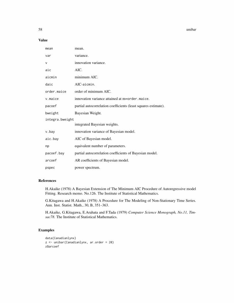
58 unibar

Value

mean mean.

var variance.


aic AIC.

aicmin minimum AIC.

daic AIC-aicmin.


v.maice innovation variance attained at m=order.maice.

pacoef partial autocorrelation coefficients (least squares estimate).

bweight Bayesian Weight.

integra.bweight

integrated Bayesian weights.

v.bay innovation variance of Bayesian model.

aic.bay AIC of Bayesian model.

np equivalent number of parameters.

pacoef.bay partial autocorrelation coefficients of Bayesian model.

arcoef AR coefficients of Bayesian model.


References

H.Akaike (1978) A Bayesian Extension of The Minimum AIC Procedure of Autoregressive modelFitting. Research memo. No.126. The Institute of Statistical Mathematics.



Examples

data(Canadianlynx)z <- unibar(Canadianlynx, ar.order = 20)z$arcoef

unimar 59

unimar Univariate Case of Minimum AIC Method of AR Model Fitting

Description

This is the basic program for the fitting of autoregressive models of successively higher by themethod of least squares realized through householder transformation.

Usage

unimar(y, max.order = NULL, plot = FALSE)

Arguments


max.order upper limit of AR order. Default is 2√n, where n is the length of the time series

y.


Details


y(t) = a(1)y(t− 1) + . . .+ a(p)y(t− p) + u(t),

where p is AR order and u(t) is Gaussian white noise with mean 0 and variance v. AIC is definedby


where n is the length of data, v is the estimates of the innovation variance and k is the number ofparameter.

Value

mean mean.

var variance.


aic AIC.

aicmin minimum AIC.

daic AIC-aicmin.


v.maice innovation variance attained at order.maice.


60 wnoise

References

G.Kitagawa and H.Akaike (1978) A Procedure For The Modeling of Non-Stationary Time Series.Ann. Inst. Statist. Math.,30, B, 351–363.


Examples

data(Canadianlynx)z <- unimar(Canadianlynx, max.order = 20)z$arcoef

wnoise White Noise Generator

Description

Generate approximately Gaussian vector white noise.

Usage

wnoise(len, perr, plot = TRUE)

Arguments

len length of white noise record.

perr prediction error.

plot logical. If TRUE (default), white noises are plotted.

Value

wnoise gives white noises.

References


Examples

# Example 1wnoise(len = 100, perr = 1)

# Example 2v <- matrix(c(1, 0, 0,

0, 2, 0,0, 0, 3), nrow = 3, ncol = 3, byrow = TRUE)

wnoise(len = 20, perr = v)

xsarma 61

xsarma Exact Maximum Likelihood Method of Scalar ARMA Model Fitting

Description

Produce exact maximum likelihood estimates of the parameters of a scalar ARMA model.

Usage

xsarma(y, arcoefi, macoefi)

Arguments


arcoefi initial estimates of AR coefficients.

macoefi initial estimates of MA coefficients.

Details

The ARMA model is given by

y(t)− a(1)y(t− 1)− . . .− a(p)y(t− p) = u(t)− b(1)u(t− 1)− ...− b(q)u(t− q),

where p is AR order, q is MA order and u(t) is a zero mean white noise.

Value

gradi initial gradient.

lkhoodi initial (-2)log likelihood.

arcoef final estimates of AR coefficients.

macoef final estimates of MA coefficients.

grad final gradient.

alph.ar final ALPH (AR part) at subroutine ARCHCK.

alph.ma final ALPH (MA part) at subroutine ARCHCK.

lkhood final (-2)log likelihood.

wnoise.var white noise variance.

References

H.Akaike (1978) Covariance matrix computation of the state variable of a stationary Gaussian pro-cess. Research Memo. No.139. The Institute of Statistical Mathematics.


62 xsarma

Examples

# "arima.sim" is a function in "stats".# Note that the sign of MA coefficient is opposite from that in "timsac".arcoef <- c(1.45, -0.9)macoef <- c(-0.5)y <- arima.sim(list(order=c(2,0,1), ar=arcoef, ma=macoef), n = 100)arcoefi <- c(1.5, -0.8)macoefi <- c(0.0)z <- xsarma(y, arcoefi, macoefi)z$arcoefz$macoef

Index

∗Topic datasetsAirpollution, 3Amerikamaru, 4bispecData, 11Blsallfood, 14Canadianlynx, 17LaborData, 28locarData, 29nonstData, 46Powerplant, 50

∗Topic packagetimsac-package, 2

∗Topic tsarmafit, 4auspec, 5autcor, 6autoarmafit, 7baysea, 8bispec, 10blocar, 12blomar, 13bsubst, 15canarm, 18canoca, 19covgen, 21decomp, 21exsar, 24fftcor, 25fpeaut, 26fpec, 27markov, 29mfilter, 31mlocar, 32mlomar, 34mulbar, 35mulcor, 37mulfrf, 38mulmar, 39mulnos, 41

mulrsp, 42mulspe, 43nonst, 45optdes, 46optsim, 47perars, 49prdctr, 51raspec, 52sglfre, 53simcon, 54thirmo, 56unibar, 57unimar, 59wnoise, 60xsarma, 61

Airpollution, 3Amerikamaru, 4arima.sim, 31armafit, 4auspec, 5autcor, 6autoarmafit, 7

baysea, 8bispec, 10, 11bispecData, 11blocar, 12, 29blomar, 4, 13Blsallfood, 14bsubst, 15, 17

Canadianlynx, 17canarm, 18canoca, 19convolve, 31covgen, 21

decomp, 14, 21

exsar, 17, 24

63

64 INDEX

fftcor, 25fpeaut, 26fpec, 27

LaborData, 28locarData, 29

markov, 29mfilter, 31mlocar, 29, 32mlomar, 34mulbar, 35, 50mulcor, 37mulfrf, 38mulmar, 39, 50mulnos, 41mulrsp, 42mulspe, 43

nonst, 45, 46nonstData, 46

optdes, 46optsim, 47

perars, 3, 49Powerplant, 50prdctr, 51print.autoarmafit (autoarmafit), 7print.blomar (blomar), 13print.fpec (fpec), 27print.mlomar (mlomar), 34print.mulcor (mulcor), 37print.perars (perars), 49print.prdctr (prdctr), 51ptint.mulspe (mulspe), 43

raspec, 52

sglfre, 53simcon, 29, 54

thirmo, 11, 56timsac (timsac-package), 2timsac-package, 2

unibar, 17, 57unimar, 17, 59

wnoise, 60

xsarma, 61

package ‘timsac’ - the comprehensive r archive network · pdf filepackage...

Documents