Pablo Cerdá-Durán University of Valencia

Kyoto, 16 November 2016

Collaborators: A. Torres-Forné, J.A. Font (U. Valencia) T. Akgün, J. Pons, J.A. Miralles (U. Alicante) M. Gabler, E. Müller (MPA) N. Stergioulas (U. Thessaloniki)

Outline

•  Magnetar magnetospheres

•  Observations and models •  Force-free twisted magnetospheres •  Magnetosphere dynamics

•  Supernova fallback and magnetic field burial

Magnetar magnetospheres

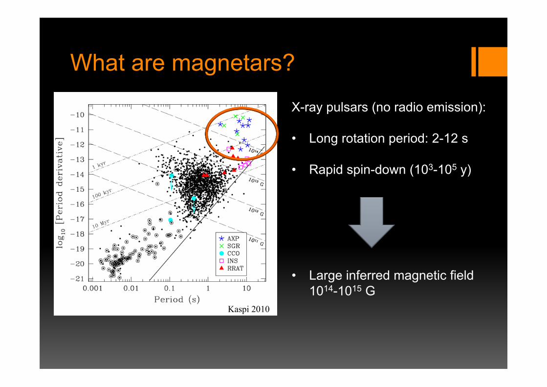
What are magnetars?

Kaspi 2010

X-ray pulsars (no radio emission):

•  Long rotation period: 2-12 s

•  Rapid spin-down (103-105 y)

•  Large inferred magnetic field 1014-1015 G

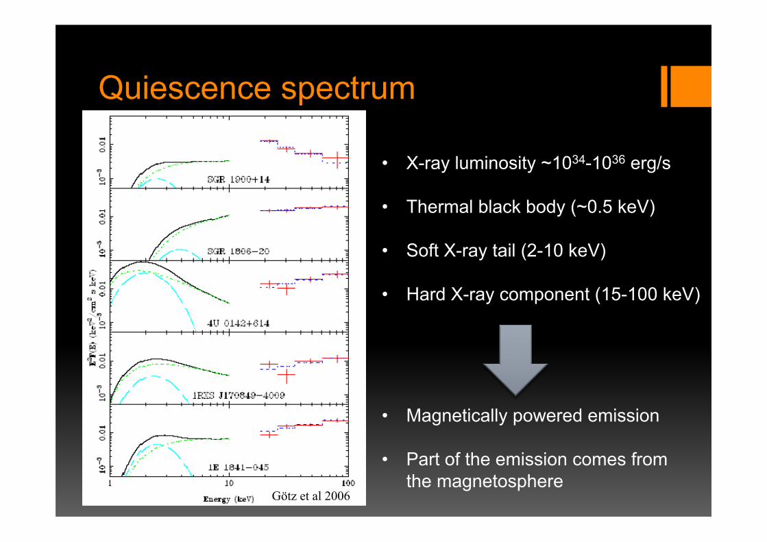
Quiescence spectrum

•  X-ray luminosity ~1034-1036 erg/s

•  Thermal black body (~0.5 keV)

•  Soft X-ray tail (2-10 keV)

•  Hard X-ray component (15-100 keV)

Götz et al 2006

•  Magnetically powered emission

•  Part of the emission comes from the magnetosphere

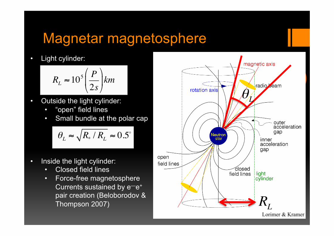
•  Light cylinder:

•  Outside the light cylinder:

•  “open” field lines •  Small bundle at the polar cap

•  Inside the light cylinder: •  Closed field lines •  Force-free magnetosphere

Currents sustained by e—e+ pair creation (Beloborodov & Thompson 2007)

Magnetar magnetosphere

Kaspi 2010

RL ≈105 P2s⎛

⎝⎜

⎞

⎠⎟km

θL ≈ R* / RL ≈ 0.5!

θL

RLLorimer & Kramer

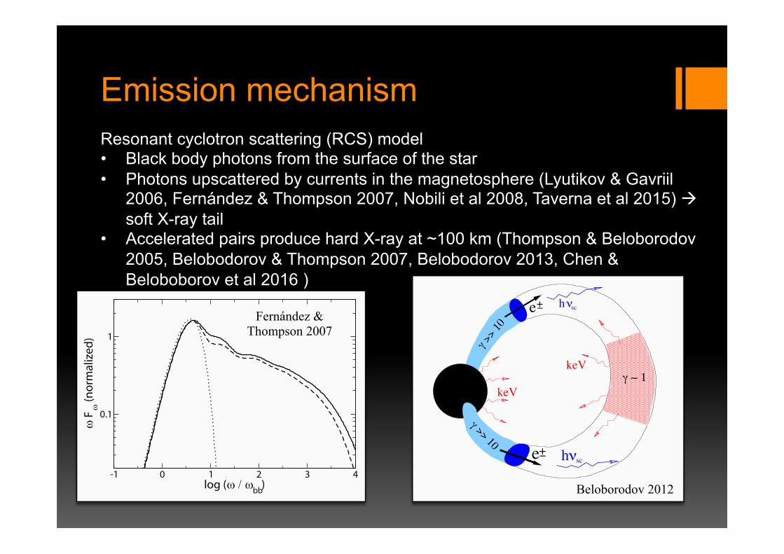
Emission mechanism Resonant cyclotron scattering (RCS) model •  Black body photons from the surface of the star •  Photons upscattered by currents in the magnetosphere (Lyutikov & Gavriil

2006, Fernández & Thompson 2007, Nobili et al 2008, Taverna et al 2015) à soft X-ray tail

•  Accelerated pairs produce hard X-ray at ~100 km (Thompson & Beloborodov 2005, Belobodorov & Thompson 2007, Belobodorov 2013, Chen & Beloboborov et al 2016 )

modes at the cyclotron resonance are comparable, because theelectromagnetic eigenmodes are determined by vacuum polari-zation effects and are linearly polarized even in the core of thecyclotron resonance (x 2). For this reason, one expects similarpulse profiles and nonthermal spectra for both polarizations ofthe seed photons. Nonetheless, the scattering cross section of anO-mode photon is suppressed with respect to that of an E-modephoton by a factor (!0) 2 (eqs. [13] and [15]; see also the discussionin Appendix A). One therefore expects the spectra to be slightlysofter and the pulsed fractions to be slightly lower when the seedphotons are injected in the O-mode.

Figure 12 shows energy spectra (left) and pulse profiles in bandV(right) using the same magnetospheric parameters, excepting thatthe seed photons are 100% polarized in the E-mode (solid curves)and the O-mode (dashed curves). In the second case, the non-thermal tail does indeed have a slightly lower amplitude com-pared with the blackbody peak, and the pulsed fraction is smaller.Nevertheless, the changes in the emission pattern resulting fromthe polarization of the seed photons are much subtler than thoseproduced by changes in the orientation of the star (xx 4.2 and4.3), offering little chance of identifying the seed photon emissionmechanism except through direct polarization measurements.

5. DISCUSSION

We have developed a Monte Carlo code to study the repro-cessing of thermal X-rays by resonant cyclotron scattering inneutron star magnetospheres using the model of Thompson et al.(2002). The code is fully three dimensional and allows for an ar-bitrary velocity distribution of the scattering particles and an ar-bitrary magnetic field geometry. Angle-dependent X-ray spectraand pulse profiles can be calculated for an arbitrary orientationbetween the magnetic axis and the spin axis and between the spinaxis and the line of sight to the star.

Our aim here has been to show which types of X-ray spectraand pulse profiles follow generically from the model and whichmay point to different emission mechanisms. We can reproducemost of the properties of the 1Y10 keVemission of the AXPs, butnot of the SGRs, by assuming a broad and mildly relativistic ve-locity distribution and moderate twist angles (!"N-S ! 0:3Y1 ra-dian). In particular, the SGRs in their most active states haveharderX-ray spectra than can be reproduced by themodel (Woodset al. 2007). Our results demonstrate that changes in the strengthof the twist and in the dynamics of the charged particles (which are

coupled strongly to the radiation field) can lead to substantialchanges in flux, hardness, pulse shape, and pulsed fraction.

5.1. Relative Strength of the Thermal and NonthermalComponents of the X-ray Spectrum

The X-ray spectra of most magnetars display a prominent ther-mal component. The corresponding blackbody area is less than, orsometimes comparable to, the expected surface area of a neutronstar (e.g.,Woods& Thompson 2006). In sources where the black-body component is dominant at !1Y3 keV, the high-energy pho-ton index is typically 2 or softer. However, SGR 1900+14presents an example of an SGR in which a thermal componentand a hard power-law component of the spectrum are simulta-neously present (Esposito et al. 2007).

Model spectra with a mildly relativistic particle distribution(kBT0 ’ 0:5mec

2, #0 ’ 0:75; eq. [19]) can easily reproduce the1Y10 keV spectra of sources like 4U 0142+614, 1RXS J170849"4009, and 1E 1841"045. Some of our model spectra show anoticeable downward break at!30Y50kBTbb ’ 10Y30 keV (e.g.,Figs. 4f and 5f ). Such a break may be present in the combinedXMM-Newton and INTEGRAL spectra of SGR 1900+14 (Gotzet al. 2006), and its presence is not excluded in other sources, suchas the AXPs 4U 0142+614 and 1E 1841"045, when one takesinto account the presence of a separately rising high-energy spec-tral component above 20 keV (Kuiper et al. 2006; Gotz et al.2006).

The quiescent SGRs have relatively weak blackbody compo-nents to their spectra, and during periods of extreme activity, apure power-law fit to the spectrum can have a photon index of!"1.6 (Mereghetti et al. 2005;Woods et al. 2007). (Even harderphoton indices are obtained from combined blackbody + power-law fits to the spectrum, but then the continuation of the 2Y10 keVfit to higher energies disagrees with the INTEGRAL flux meas-urements.) We could obtain spectra as hard as this by choosing abroad power-law momentum distribution for the magnetosphericcharges (Fig. 6), but the output spectrum then displays a strongblackbody component. In the fit of Esposito et al. (2007) for SGR1900+14, the amplitude of the blackbody component is about3 times that of the power-law component at the blackbody peak,whereas in the spectra of Figure 6b, it is 6Y8 times larger.

We expect this conclusion to hold for any model for the high-energy continuum that relies on the upscattering of the thermalseed photons. Balancing the energy input to the coronal charges

Fig. 12.—Energy spectra (left) and band V pulse profile (right) corresponding to 100% polarization of the seed photons in the E-mode (solid curves) and the O-mode(dashed curves). The velocity distribution is monoenergetic and unidirectional (eq. [36]) withmean drift speed # ¼ 0:7 and total width!# ¼ 0:1. In addition,!"N-S ¼ 1and !" ¼ ! los ¼ 0.

QUIESCENT X-RAY EMISSION OF MAGNETARS 635

Fernández & Thompson 2007

2

sc+−

e+−

keV

keV

hνsc

hνeγ >> 10

γ >>

10

γ ∼ 1

Figure 1. Sketch of an activated magnetic loop. Relativisticparticles are injected near the star where B > BQ = 4.4× 1013 G.Large e± multiplicity M ∼ 100 (Equation 11) develops in the adi-abatic zone B > 1013 G (shaded in blue). The outer part of theloop is in the radiative zone; here the scattered photons of energyE = hνsc escape and form the hard X-ray spectrum that is cal-culated in Section 3. The outflow decelerates (and annihilates) atthe top of the loop, shaded in pink; here it becomes very opaque tothe thermal keV photons flowing from the star. Photons reflectedfrom the pink region have the best chance to be upscattered by therelativistic outflow in the lower parts of the loop, and control itsdeceleration (Section 2.2).

generates relativistic particles near the magnetar whereB > 1013 G. We here briefly describe the expectedsource.Like the sun, magnetars are believed to have twisted

magnetospheres that are deformed by surface motions(Thompson et al. 2000; 2002). Beloborodov (2009, here-after B09) developed electrodynamic theory for the dis-sipative, twisted magnetosphere attached to a conduct-ing sphere (neutron star). The theory predicts that themagnetic twist concentrates on field lines that extend farfrom the conducting star, forming an extended bundleof electric currents. This “j-bundle” is heated by ohmicdissipation and emits radiation. The currents are nearlyforce-free, j × B = 0, and sustained by a longitudinalvoltage Φ along the magnetic field lines. Net current cir-culating through the magnetosphere, I, generates ohmicpower L = IΦ that feeds the observed activity.Similar ohmic heating occurs in ordinary pulsars, and

it may be useful to compare them with magnetars. Inordinary pulsars, the magnetospheric twist is pumped atthe light cylinder by the rotation of the star, and ohmicdissipation occurs on the open field lines. The electriccurrent is then roughly given by I ∼ cµ/R2

lc (where Rlcis the light-cylinder radius and µ is the magnetic dipolemoment of the star), and voltage Φ can exceed 1012 V.The dissipated power IΦ is always smaller than the spin-down luminosity of the star. In magnetars, surface mo-tions twist the closed magnetosphere. Then the electriccurrent may be as large as I ∼ cµ/R2, where R is thestar radius. The characteristic voltage is Φ ∼ 109 V (Be-loborodov & Thompson 2007). The dissipated power IΦis typically much larger than the spindown power.Ohmic dissipation tends to gradually remove electric

currents from the closed magnetosphere as described inB09. This process creates a growing “cavity” with van-ished current density j = 0. The currents have longest

lifetimes on magnetic field lines with large apex radiiRmax ≫ R. As a result, the magnetospheric activitybecomes confined to the bundle of extended field lines.This theoretical picture agrees with observations (see Be-loborodov 2011 for a review).Consider magnetic field lines that extend sufficiently

far from the star into the region where B is smaller thana given value B1. Luminosity that can be generated onthese field lines may be estimated as follows. Approxi-mating magnetic field by a dipole configuration with adipole moment µ, one finds that the field lines reachingthe region B < B1 carry the magnetic flux !1 = 2πµ/R1

filling the hemisphere of radius R1 = (µ/B1)1/3. If thefield lines are twisted with amplitude ψ, they must carryelectric current (according to Stokes theorem, see B09and Appendix C),

I1 ≈ cψ!1

8πR1=

c µψ

4R21

. (1)

The twist amplitude ψ is measured in radians. It has themeaning of relative azimuthal position of the northernand southern footpoints of the magnetospheric field line.The generated power is L = I1Φ, which yields

L ≈ 1036 ψ

(

µ

1033 G cm2

)1/3 ( Φ

4× 109 V

)

×(

B1

1012 G

)2/3

erg s−1. (2)

Strong twists tend to inflate the magnetosphere (Wolfson1995; Parfrey et al. 2012a,b). As long as ψ <∼ 1, thiseffect is modest (it scales as ψ2 at ψ < 1, see B09), andthe poloidal field may be well approximated by a dipoleconfiguration with dipole moment µ.

2.2. Interaction of outflowing particles with radiationfield

Discharge with voltage Φ ∼ 109 V injects electrons (orpositrons) with high Lorentz factors γ ∼ eΦ/mec2 ∼ 103.The relativistic plasma created near the star expandsalong the magnetic field and forms a relativistic out-flow, resembling the outflow along open field lines in or-dinary pulsars (however, here plasma moves along closedfield lines and is trapped in the magnetic loops aroundthe neutron star). Magnetars are hot and bright; theirdense radiation exerts a strong drag on the magneto-spheric particles and controls the outflow velocity. Onthe other hand, the plasma significantly changes the ra-diation field around the magnetar. The interaction of theflowing e± plasma and radiation may be described as aself-consistent radiative transfer problem. This problemis solved numerically in the accompanying paper (Be-loborodov, in preparation, hereafter B12). The resultscan be summarized as follows.The outflow interacts with radiation via resonant scat-

tering; other processes turn out unimportant. Consideran outflowing electron (or positron) with Lorentz fac-tor γ = (1 − β2)−1/2, and a target photon of energy Etpropagating at an angle ϑ with respect to the outflowdirection. Resonant scattering can occur if the photonenergy in the electron rest frame,

E = γ(1− β cosϑ)Et, (3)

Beloborodov 2012

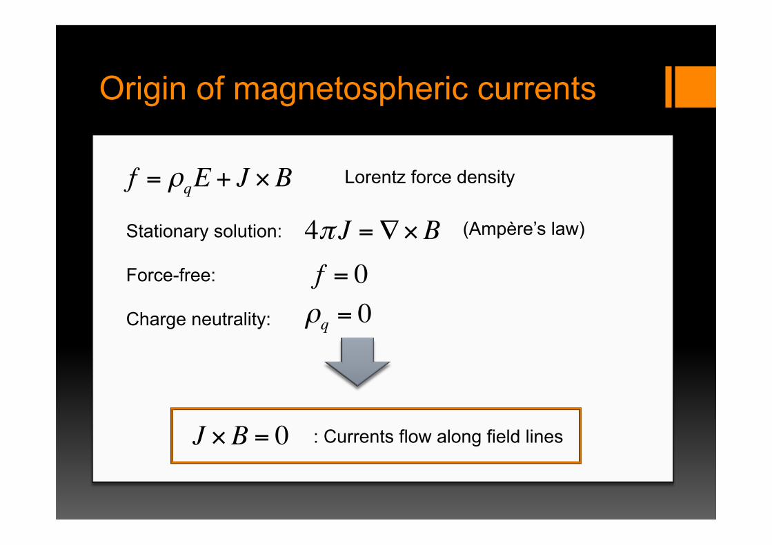
Origin of magnetospheric currents

f = ρqE + J ×B Lorentz force density

ρq = 0

J ×B = 0

Stationary solution: Force-free: Charge neutrality:

f = 04π J =∇×B (Ampère’s law)

: Currents flow along field lines

Origin of magnetospheric currents

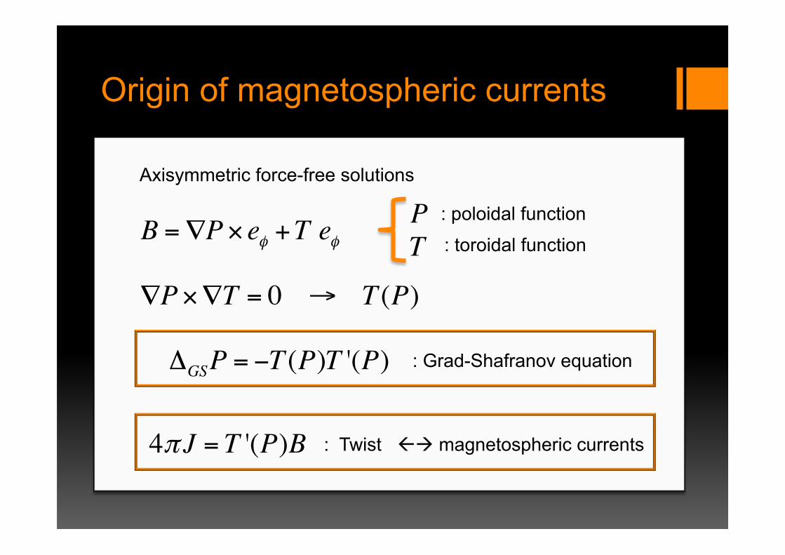
Axisymmetric force-free solutions

: Twist ßà magnetospheric currents

B =∇P× eφ +T eφPT

: poloidal function

: toroidal function

∇P×∇T = 0 → T (P)

ΔGSP = −T (P)T '(P)

4π J = T '(P)B

: Grad-Shafranov equation

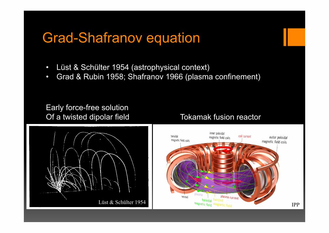
Grad-Shafranov equation

•  Lüst & Schülter 1954 (astrophysical context) •  Grad & Rubin 1958; Shafranov 1966 (plasma confinement)

IPP

1954ZA.....34..263L

Lüst & Schülter 1954

Tokamak fusion reactor Early force-free solution Of a twisted dipolar field

Variability •  Repeated burst activity: 1042 erg/s in

0.01-1 s •  Giant flares (3):

Ø  Initial spike: 1044 – 1047 erg/s in 0.25-0.5 s

Ø  Pulsating tail: 1044 erg/s in 200-400 s •  Long term variability: hours to years

Strohmayer & Watts 2006

Merghetti et al 2005 1E 1048-59, Woods et al 2004

Untwisting magnetospheres

•  Twisted magnetospheres are not static à energy loses by radiation •  Magnetospheres untwist in secular time-scales (Beloborodov 2009,

2012, Chen & Beloborodov 2016) •  Pair plasma flowing along twisted field linesà hot spot at the surface •  Twisted field at ~100km à magnetar corona à hard X-ray component

Model ingredients: -  Thermal emission from the surface -  Current distribution at the magnetosphere

-  Force-free magnetic field configuration -  e- and e+ momentum/spatial distribution: multiplicity?

-  Back-reaction: -  Photon flux ßà e- and e+ distribution -  Hot spots

Burst models

Internal mechanism: •  Reach breaking strain ~0.1 (Horowitz &

Kadau 2009) •  “Crustquake” (Thompson & Duncan 1996) •  Mechanical failure may propagates too

slow (Levin & Lyutikov 2012, Belobodorov & Levin 2014, Li et al 2016)

Magneto-thermal evolution of the crust (Perna & Pons 2011) •  Hall drift timescale ~ 103-104 yr •  Stress builds in the crust

Duncan/Thompson & Duncan 2001

External mechanism: •  Stress bulid-up limited by plastic deformations •  Highly twisted magnetosphere leads to

magnetic reconnection event •  Solar-like flare (Lyutikov 2006, Masada et al

2010, Lyutikov 2014)

Masada et al 2010

Maximum magnetospheric twist MHD dynamical calculations (Mikic & Linker 1994, Parfrey et al 2013) •  Maximum strain ~ maximum twist ~1 – 4 rad •  Results sensitive to:

Mikic & Linker 1994

1994ApJ...430..898M

1994ApJ...430..898M

-  How fast you twist the magnetosphere

-  Resistivity -  Magnetic field configurarion -  Twist profile

Can we learn something from force-free equilibrium models?

Force-free twisted magnetospheres

Force-free magnetospheres Akgün, Miralles, Pons & CD, MNRAS, 462, 1894 (2016)

: Twist ßà magnetospheric currents

ΔGSP = −T (P)T '(P)

4π J = T '(P)B

: Grad-Shafranov equation

T (P) : Toroidal function à fixed by the field at the NS surface

Non-linear elliptic equation à iterative numerical method (needs initial guess)

Toroidal function

Pc

Twist

-  Solutions of the GS equation with twist larger than ~1 cannot be found -  This limit is similar to dynamical simulations. -  Is this limit related to the stability of the solution?

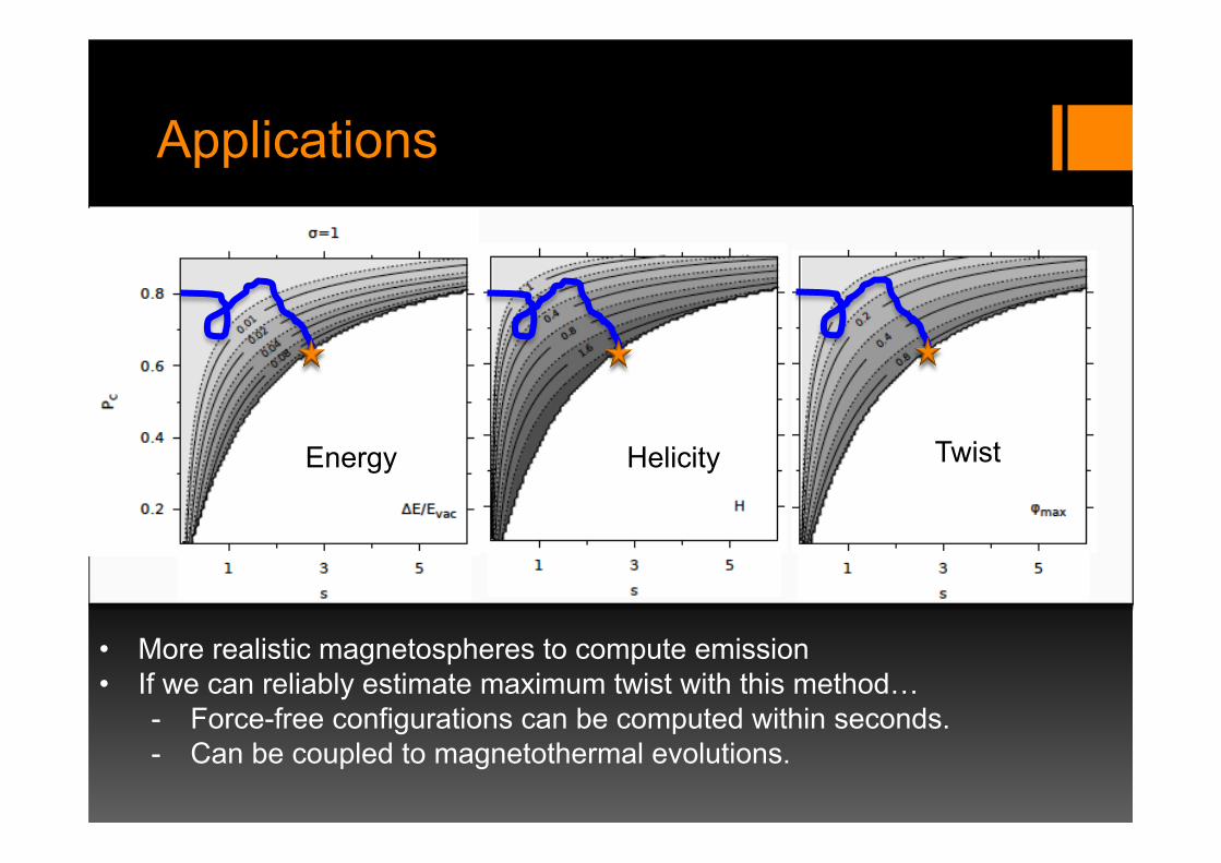
Applications

•  More realistic magnetospheres to compute emission •  If we can reliably estimate maximum twist with this method…

-  Force-free configurations can be computed within seconds. -  Can be coupled to magnetothermal evolutions.

Energy Helicity Twist

Uniqueness of the solution

ΔGSP = −T (P)T '(P) : Grad-Shafranov equation

ΔGSP = 0•  Current free (potential solutions):

+ boundary conditions àUnique solution

•  Linear perturbations in à Unique solution (see e.g. Gabler et al 2014): potential solution + T (P)

•  Bineau 1972 proved uniqueness for sufficiently small twist

T (P)

•  General case: it is not possible to use a maximum principle to prove uniqueness of the solution.

Solution may not be unique above certain threshold twist

Uniqueness of the solution?

NSs with twisted magnetosphere in GR 7

-50 0 50

-50

0

50

0.0 0.2 0.4 0.6 0.8 1.0

-30

-20

-10

0

10

20

30Btor | Bpol

R(km

)

-30

-20

-10

0

10

20

30

R(km

)

-30 -20 -10 0 10 20 30-30

-20

-10

0

10

20

30

R(km

)

-30

-20

-10

0

10

20

30

R(km

)

-40

-20

0

20

40Btor | Bpol

-40

-20

0

20

40-40

-20

0

20

40

-40 -20 0 20 40-40

-20

0

20

40

-50

0

50

Btor | Bpol

-50

0

50

-50

0

50

0.0 0.2 0.4 0.6 0.8 1.0 0.0 0.2 0.4 0.6 0.8 1.0

Figure 2. TT magnetosphere configurations: strength of the toroidal (left half of each panel) and poloidal (right half of each panel) magnetic field. The leftcolumn shows models with λ = 2, the central column those with λ = 3, and the right column those with λ = 6. Contours represents magnetic field surfaces.From top to bottom each row corresponds to increasing values of a,given in Table 1. For each panel the colour code is normalized to the maximum value ofthe magnetic field components that are listed in table 1. The blue line represents the surface of the star. The red line locates the boundary of the region wherethe toroidal component of the magnetic field is present.

Pili et al 2015 Akgün et al 2015

Discrepancy in force-free configurations for similar boundary conditions: -  Pili et al 2015 found different topologies of the magnetic field -  Are we facing a problem with non-unique solution?

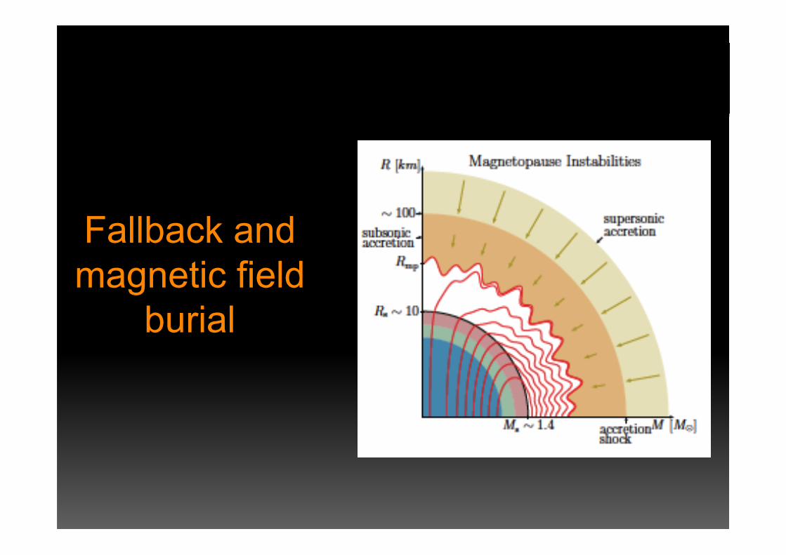
Fallback and magnetic field

burial

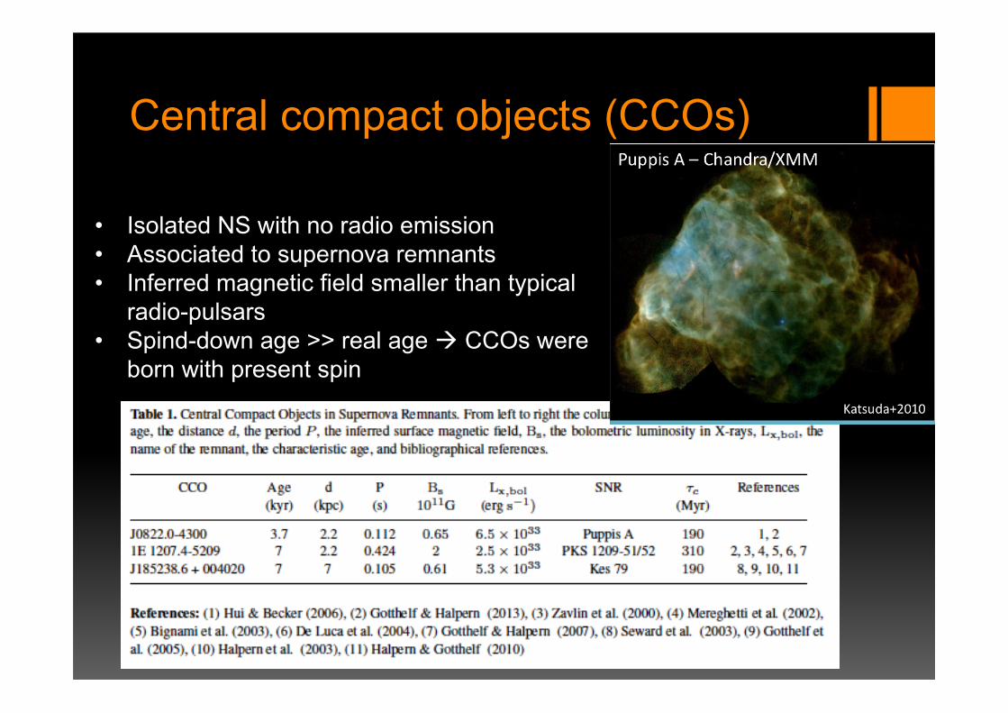
Central compact objects (CCOs)

•  Isolated NS with no radio emission •  Associated to supernova remnants •  Inferred magnetic field smaller than typical

radio-pulsars •  Spind-down age >> real age à CCOs were

born with present spin

CCO models

Ho 2015

Hidden magnetic field model •  Magnetic field buried by SN fallback •  Re-emergence of the magnetic field in 1-107 kyr

(Young & Chanmugan 1995, Muslimov & Page 1995, Geppert et al. 1999, Shabaltas & Lai 2012, Ho 2011, Viganò & Pons 2012, Ho 2015).

•  CCOs could be evolutionary linked to braking index pulsars (Ho 2015)

“Anti-magnetar” model (Halpern et al 2007) •  Born with low magnetic field •  Slowly rotating progenitors •  Numerical simulations show non-

rotating progenitors can produce pulsar-like magnetic fields (Endeve et al 2012, Obergaulinger et al 2014)

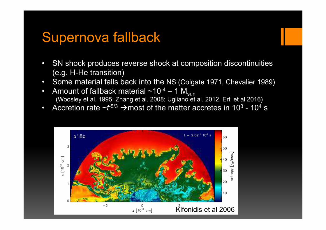
Supernova fallback

•  SN shock produces reverse shock at composition discontinuities (e.g. H-He transition)

•  Some material falls back into the NS (Colgate 1971, Chevalier 1989) •  Amount of fallback material ~10-4 – 1 Msun

(Woosley et al. 1995; Zhang et al. 2008; Ugliano et al. 2012, Ertl et al 2016) •  Accretion rate ~t-5/3 àmost of the matter accretes in 103 - 104 s

Kifonidis et al 2006

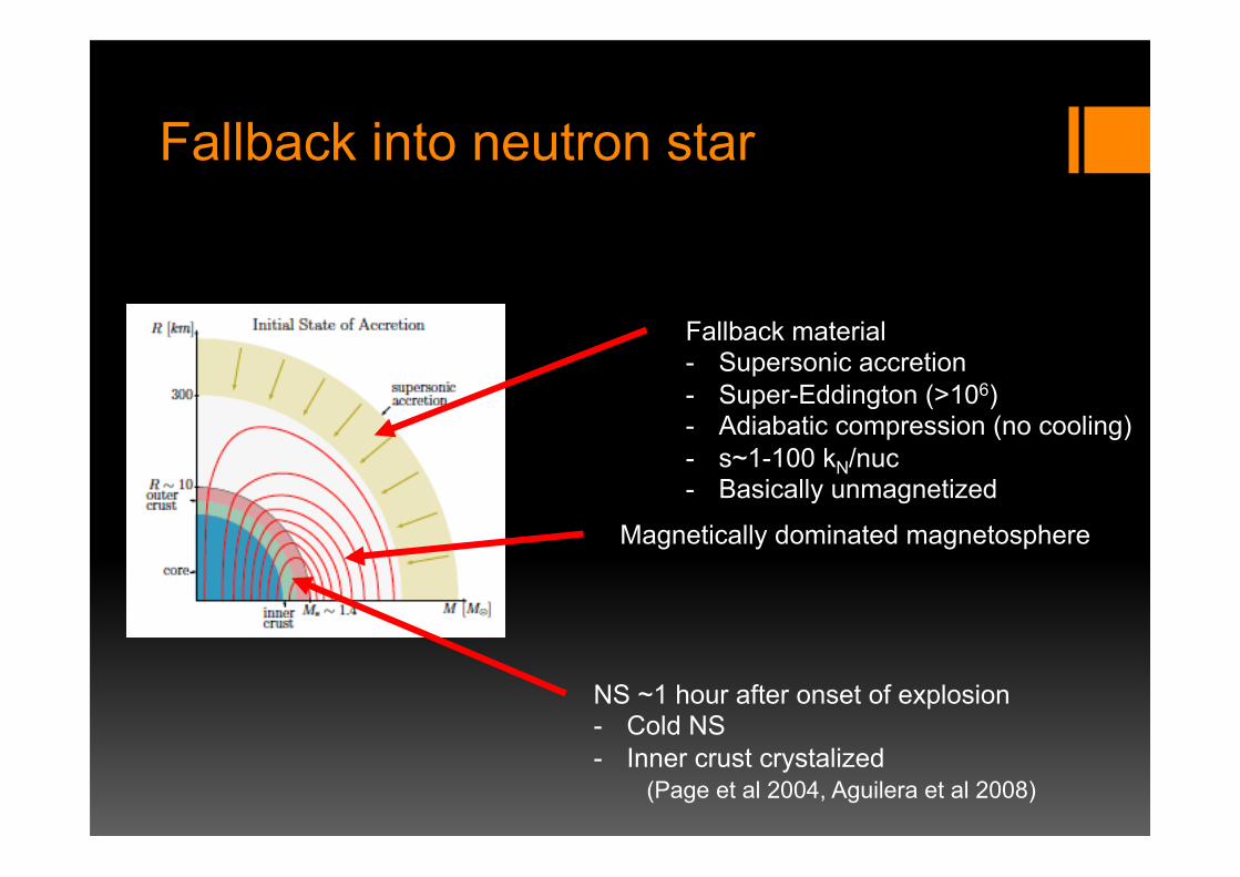
Fallback into neutron star

Fallback material -  Supersonic accretion -  Super-Eddington (>106) -  Adiabatic compression (no cooling) -  s~1-100 kN/nuc -  Basically unmagnetized

Magnetically dominated magnetosphere

NS ~1 hour after onset of explosion -  Cold NS -  Inner crust crystalized

(Page et al 2004, Aguilera et al 2008)

Accretion shock formation

•  Accretion shock is formed as the shock is slowed down by the NS surface or the compressed magnetosphere (Chevalier 1989)

•  The shock stalls at about 107-108 km (Houck et al 1991)

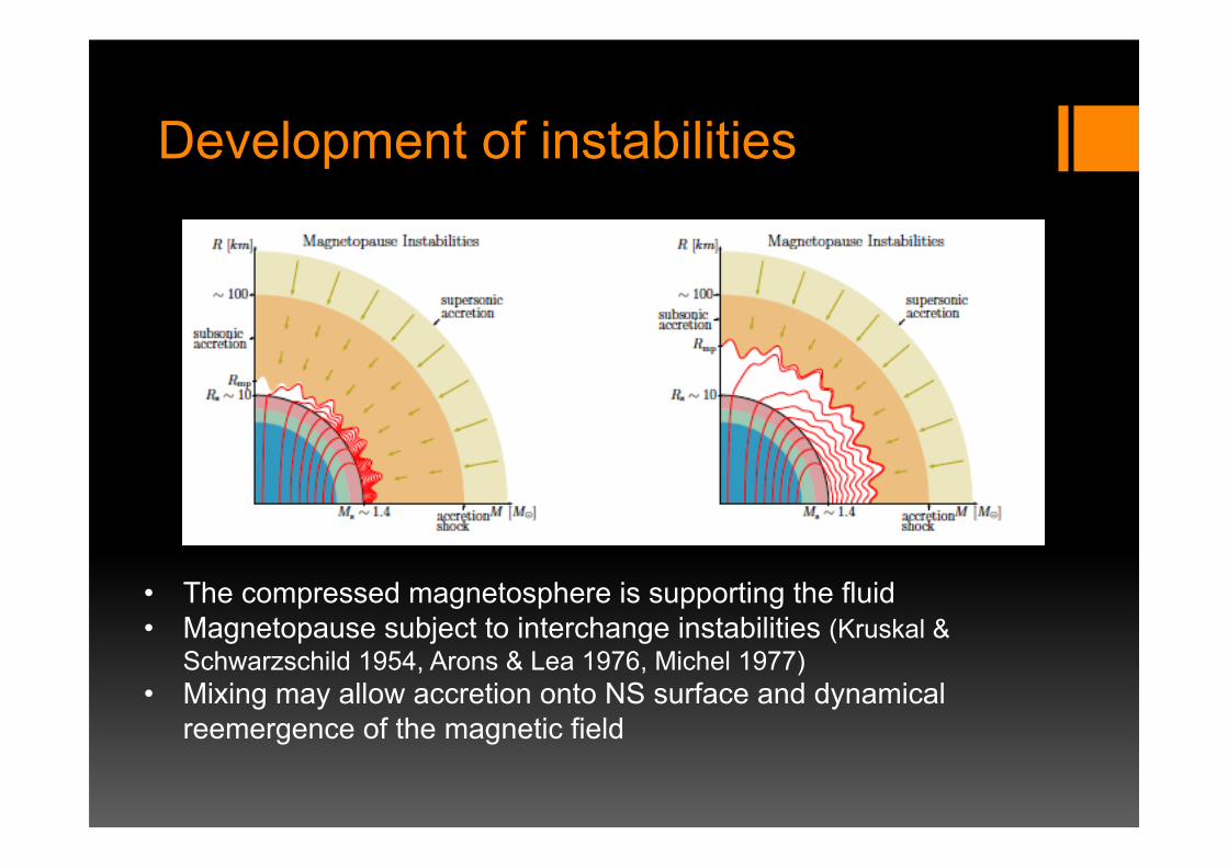
Development of instabilities

•  The compressed magnetosphere is supporting the fluid •  Magnetopause subject to interchange instabilities (Kruskal &

Schwarzschild 1954, Arons & Lea 1976, Michel 1977) •  Mixing may allow accretion onto NS surface and dynamical

reemergence of the magnetic field

End of the accretion phase

•  High accretion / low B field - instability vertical scale << burial depth - Buried field

•  Low accretion / high B field -  Instability vertical scale >> burial depth -  Dynamical reemergence à non buried field?

Previous works •  Local MHD simulations •  Simplified geometries •  Difficult to resolve numerically all relevant regimes

(see later)

Increasing accretion rate

Bernal et al 2013

•  Payne & Melatos (2004, 2007) •  Bernal et al. (2010, 2013); •  Mukherjee et al (2013a,b)

Our work (Torres-Forné et al 2016)

instability vertical scale vs burial depth

•  Simple model: easy to explore parameter space

•  Covers different regimes with similar accuracy

•  Burial condition do not depend on details of the instabilities

•  Non-buried case may depend on details of the inestabilities

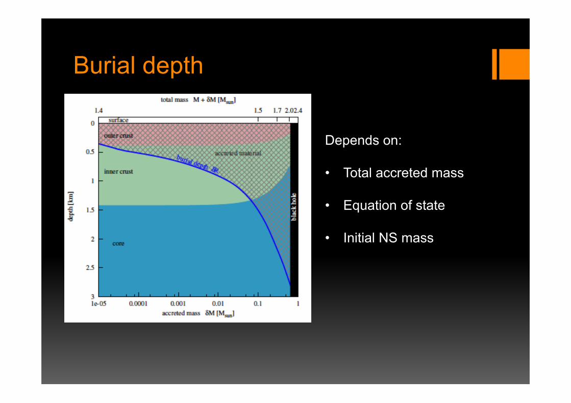
Burial depth

Depends on: •  Total accreted mass

•  Equation of state

•  Initial NS mass

Compressed magnetosphere •  Force-free magnetosphere (potential solution) compressed by

spherically accreting matter (non-dynamic)

•  We use different configurations for the NS field

•  Magnetic pressure increases as magnetosphere is compressed

•  Magnetic pressure is highest at the equator

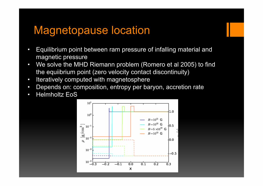
Magnetopause location •  Equilibrium point between ram pressure of infalling material and

magnetic pressure •  We solve the MHD Riemann problem (Romero et al 2005) to find

the equiibrium point (zero velocity contact discontinuity) •  Iteratively computed with magnetosphere •  Depends on: composition, entropy per baryon, accretion rate •  Helmholtz EoS

Instability vertical scale

Magnetopause height over NS ~ instability vertical scale

Interchange instability (Kruskal & Schwarzschild 1954): •  All wavelengths are unstable •  Instability limited by the height of the magnetosphere

Exploring the parameter space •  Typical pulsar is easily buried by falback •  Very difficult to bury magnetar fields

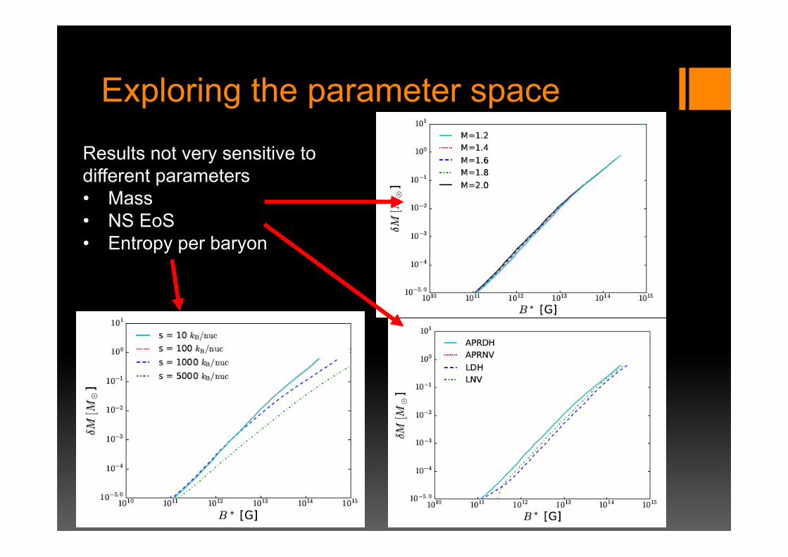
Exploring the parameter space

Results not very sensitive to different parameters •  Mass •  NS EoS •  Entropy per baryon

Conclusions

•  Force-free magnetosphere models matching NS interior fields à  emission mechanism à  Magnetothermal evolution à  Possible estimation of reconnection events

•  Internal magnetar oscillations couple to the magnetosphere à QPO modulation mechanism à 1:3:5 frequencies ßà odd/even symmetry

•  CCOs: Buried magnetic field scenario is plausible