p. coleman 1 center for materials theory, rutgers ... · 1 center for materials theory, rutgers...
TRANSCRIPT

arX
iv:c
ond-
mat
/061
2006
v3 [
cond
-mat
.str
-el]
3 J
an 2
007
Heavy Fermions: electrons at the edge of magnetism
P. Coleman1
1 Center for Materials Theory, Rutgers University, Piscataway, NJ 08855, U.S.A.
Abstract
An introduction to the physics of heavy fermion compounds is presented, highlighting the
conceptual developments and emphasizing the mysteries and open questions that persist
in this active field of research.
This article is a contribution to volume 1 of the Handbook of Magnetism and
Advanced Magnetic Materials, edited by Helmut Kronmuller and Stuart Parkin, to
be published by John Wiley and Sons, Ltd.
keywords: Heavy Fermion, Superconductivity, Local Moments, Kondo effect,
Quantum Criticality.
1

Contents
I. Introduction: “Asymptotic Freedom” in a Cryostat. 3
A. Brief History 6
B. Key elements of Heavy Fermion Metals 11
1. Spin entropy: a driving force for new physics 11
2. “Local” Fermi liquids with a single scale 14
II. Local moments and the Kondo lattice 21
A. Local Moment Formation 21
1. The Anderson Model 21
2. Adiabaticity and the Kondo resonance 24
B. Hierachies of energy scales 27
1. Renormalization Concept 27
2. Schrieffer Wolff transformation 29
3. The Kondo Effect 30
4. Doniach’s Kondo Lattice Concept 33
C. The Large N Kondo Lattice 37
1. Gauge theories, Large N and strong correlation. 37
2. Mean field theory of the Kondo lattice 39
3. The charge of the f-electron. 45
4. Optical Conductivity of the heavy electron fluid. 48
D. Dynamical Mean Field Theory. 51
III. Kondo Insulators 55
A. Renormalized Silicon 55
B. Vanishing of RKKY interactions 59
C. Nodal Kondo Insulators 59
IV. Heavy Fermion Superconductivity 61
A. A quick tour 61
B. Phenomenology 64
C. Microscopic models 68
1. Antiferromagnetic fluctuations as a pairing force. 68
2. Towards a unified theory of HFSC 73
V. Quantum Criticality 77
A. Singularity in the Phase diagram 77
B. Quantum, versus classical criticaltiy. 80
C. Signs of a new universality. 83
1. Local quantum criticality 84
2. Quasiparticle fractionalization and deconfined criticality. 85
2
3. Schwinger Bosons 86
VI. Conclusions and Open Questions 87
References 89
I. INTRODUCTION: “ASYMPTOTIC FREEDOM” IN A CRYOSTAT.
The term “heavy fermion ” was coined by Steglich, Aarts et al (Steglich et al., 1976) in the late
seventies to describe the electronic excitations in a new class of inter-metallic compound with an
electronic density of states as much as 1000 times larger than copper. Since the original discovery of
heavy fermion behavior in CeAl3 by Andres, Graebner and Ott (Andres et al., 1975), a diversity of
heavy fermion compounds, including superconductors, antiferromagnets and insulators have been
discovered. In the last ten years, these materials have become the focus of intense interest with the
discovery that inter-metallic antiferromagnets can be tuned through a quantum phase transition
into a heavy fermion state by pressure, magnetic fields or chemical doping (von Lohneysen, 1996;
von Lohneysen et al., 1994; Mathur et al., 1998). The “quantum critical point” that separates the
heavy electron ground state from the antiferromagnet represents a kind of singularity in the material
phase diagram that profoundly modifies the metallic properties, giving them a a pre-disposition
towards superconductivity and other novel states of matter.
One of the goals of modern condensed matter research is to couple magnetic and electronic
properties to develop new classes of material behavior, such as high temperature superconductiv-
ity or colossal magneto-resistance materials, spintronics, and the newly discovered multi-ferroic
materials. Heavy electron materials lie at the very brink of magnetic instability, in a regime where
quantum fluctuations of the magnetic and electronic degrees are strongly coupled As such, they
are an important test-bed for the development of our understanding about the interaction between
magnetic and electronic quantum fluctuations.
Heavy fermion materials contain rare earth or actinide ions forming a matrix of localized mag-
netic moments. The active physics of these materials results from the immersion of these magnetic
moments in a quantum sea of mobile conduction electrons. In most rare earth metals and insula-
tors, local moments tend to order antiferromagnetically, but in heavy electron metals, the quantum
mechanical jiggling of the local moments induced by delocalized electrons is fierce enough to melt
the magnetic order.
The mechanism by which this takes place involves a remarkable piece of quantum physics called
3

the “Kondo effect” (Jones, 2007; Kondo, 1962, 1964). The Kondo effect describes the process by
which a free magnetic ion, with a Curie magnetic susceptibility at high temperatures, becomes
screened by the spins of the conduction sea, to ultimately form a spinless scattering center at low
temperatures and low magnetic fields. (Fig. 1 a.). In the Kondo effect this screening process is
continuous, and takes place once the magnetic field, or the temperature drops below a characteristic
energy scale called the Kondo temperature TK . Such “quenched” magnetic moments act as strong
elastic scattering potentials for electrons, which gives rise an increase in resistivity produced by
isolated magnetic ions. When the same process takes place inside a heavy electron material, it
leads to a spin quenching at every site in the lattice, but now, the strong scattering at each site
develops coherence, leading to a sudden drop in the resistivity at low temperatures. (Fig 1 (b)).
Heavy electron materials involve the dense lattice analog of the single ion Kondo effect and are
often called “Kondo lattice” compounds (Doniach, 1977). In the lattice, the Kondo effect may
be alternatively visualized as the dissolution of localized, and neutral magnetic f spins into the
quantum conduction sea, where they become mobile excitations. Once mobile, these free spins
acquire charge and form electrons with a radically enhanced effective mass (Fig. 2). The net effect
of this process, is an increase in the volume of the electronic Fermi surface, accompanied by a
FIG. 1 (a) In the Kondo effect, local moments are free at high temperatures and high fields, but become
“screened” at temperatures and magnetic fields that are small compared with the “Kondo temperature” TK
forming resonant scattering centers for the electron fluid. The magnetic susceptibility χ changes from a Curie
law χ ∼ 1T at high temperature, but saturates at a constant paramagnetic value χ ∼ 1
TKat low temperatures
and fields. (b)The resistivity drops dramatically at low temperatures in heavy fermion materials, indicating
the development of phase coherence between the scattering off the lattice of screened magnetic ions. (After
(Smith and Riseborough, 1985))
4
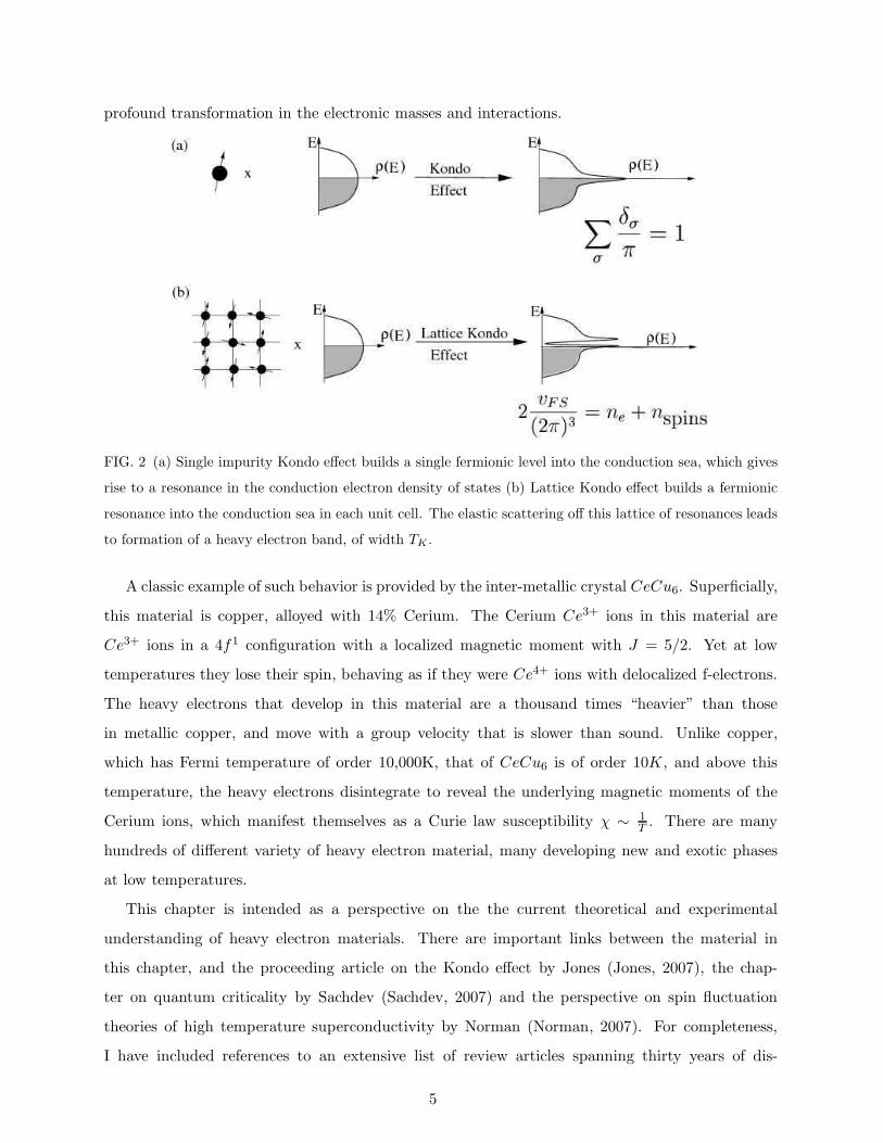
profound transformation in the electronic masses and interactions.
FIG. 2 (a) Single impurity Kondo effect builds a single fermionic level into the conduction sea, which gives
rise to a resonance in the conduction electron density of states (b) Lattice Kondo effect builds a fermionic
resonance into the conduction sea in each unit cell. The elastic scattering off this lattice of resonances leads
to formation of a heavy electron band, of width TK .
A classic example of such behavior is provided by the inter-metallic crystal CeCu6. Superficially,
this material is copper, alloyed with 14% Cerium. The Cerium Ce3+ ions in this material are
Ce3+ ions in a 4f1 configuration with a localized magnetic moment with J = 5/2. Yet at low
temperatures they lose their spin, behaving as if they were Ce4+ ions with delocalized f-electrons.
The heavy electrons that develop in this material are a thousand times “heavier” than those
in metallic copper, and move with a group velocity that is slower than sound. Unlike copper,
which has Fermi temperature of order 10,000K, that of CeCu6 is of order 10K, and above this
temperature, the heavy electrons disintegrate to reveal the underlying magnetic moments of the
Cerium ions, which manifest themselves as a Curie law susceptibility χ ∼ 1T . There are many
hundreds of different variety of heavy electron material, many developing new and exotic phases
at low temperatures.
This chapter is intended as a perspective on the the current theoretical and experimental
understanding of heavy electron materials. There are important links between the material in
this chapter, and the proceeding article on the Kondo effect by Jones (Jones, 2007), the chap-
ter on quantum criticality by Sachdev (Sachdev, 2007) and the perspective on spin fluctuation
theories of high temperature superconductivity by Norman (Norman, 2007). For completeness,
I have included references to an extensive list of review articles spanning thirty years of dis-
5
covery, including books on the Kondo effect and heavy fermions (Cox and Zawadowski, 1999;
Hewson, 1993), general reviews on heavy fermion physics (Fulde et al., 1988; Grewe and Steglich,
1991; Lee et al., 1986; Ott, 1987; Stewart, 1984), early views of Kondo and mixed valence physics
(Gruner and Zawadowski, 1974; Varma, 1976), the solution of the Kondo impurity model by renor-
malization group and the strong coupling expansion (Nozieres and Blandin, 1980; Wilson, 1976),
the Bethe Ansatz method (Andrei et al., 1983; Tsvelik and Wiegman, 1983), heavy fermion super-
conductivity (Cox and Maple, 1995; Sigrist and Ueda, 1991a), Kondo insulators (Aeppli and Fisk,
1992; Riseborough, 2000; Tsunetsugu et al., 1997), X-ray spectroscopy (Allen et al., 1986), op-
tical response in heavy fermions (DeGiorgi, 1999) and the latest reviews on non-Fermi liquid
behavior and quantum criticality (Coleman et al., 2001; Flouquet, 2005; von Lohneysen et al.,
2007; Miranda and Dobrosavljevic, 2005; Stewart, 2001; Varma et al., 2002). There are inevitable
apologies, for this article is highly selective and partly because of lack of lack of space does not
cover dynamical mean field theory approaches to heavy fermion physics (Cox and Grewe, 1988;
Georges et al., 1996; Jarrell, 1995; Vidhyadhiraja et al., 2003), nor the extensive literature on the
order-parameter phenomenology of heavy fermion superconductors reviewed in (Sigrist and Ueda,
1991a).
A. Brief History
Heavy electron materials represent a frontier in a journey of discovery in electronic and magnetic
materials that spans more than 70 years. During this time, the concepts and understanding have
undergone frequent and often dramatic revision.
In the early 1930’s de Haas et al. (de Haas et al., 1933) in Leiden, discovered a “resistance
minimum” that develops in the resistivity of copper, gold, silver and many other metals at low
temperatures (Fig. 3). It took a further 30 years before the purity of metals and alloys improved
to a point where the resistance minimum could be linked to the presence of magnetic impurities
(Clogston et al., 1962; Sarachik et al., 1964). Clogston, Mathias and collaborators at Bell Labs
(Clogston et al., 1962) found they could tune the conditions under which iron impurities in Niobium
were magnetic, by alloying with Molybdenum. Beyond a certain concentration of Molybdenum,
the iron impurities become magnetic and a resistance minimum was observed to develop.
In 1961, Anderson formulated the first microscopic model for the formation of magnetic moments
in metals. Earlier work by Blandin and Friedel (Blandin and Friedel, 1958) had observed that
localized d states form resonances in the electron sea. Anderson extended this idea and added a
6

FIG. 3 (a) Resistance minimum in MoxNb1−x after (Sarachik et al., 1964) (b) Temperature dependence of
excess resistivity produced by scattering off a magnetic ion, showing universal dependence on a single scale,
the Kondo temperature. Original data from (White and Geballe, 1979)
new ingredient: the Coulomb interaction between the d-electrons, which he modeled by term
HI = Un↑n↓. (1)
Anderson showed that local moments formed once the Coulomb interaction U became large. One
of the unexpected consequences of this theory, is that local moments develop an antiferromagnetic
coupling with the spin density of the surrounding electron fluid, described by the interaction
(Anderson, 1961; Coqblin and Schrieffer, 1969; Kondo, 1962, 1964; Schrieffer and Wolff, 1966)
HI = J~σ(0) · ~S (2)
where ~S is the spin of the local moment and ~σ(0) is the spin density of the electron fluid. In Japan,
Kondo (Kondo, 1962) set out to examine the consequences of this result. He found that when he
calculated the scattering rate 1τ of electrons off a magnetic moment to one order higher than Born
approximation,
1
τ∝
[
Jρ+ 2(Jρ)2 lnD
T
]2
, (3)
where ρ is the density of state of electrons in the conduction sea and D is the width of the
electron band. As the temperature is lowered, the logarithmic term grows, and the scattering rate
and resistivity ultimately rises, connecting the resistance minimum with the antiferromagnetic
interaction between spins and their surroundings.
A deeper understanding of the logarithmic term in this scattering rate required the renor-
malization group concept (Anderson and Yuval, 1969, 1970, 1971; Fowler and Zawadowskii, 1971;
Nozieres, 1976; Nozieres and Blandin, 1980; Wilson, 1976). The key idea here, is that the physics
7
of a spin inside a metal depends on the energy scale at which it is probed. The “Kondo” effect
is a manifestation of the phenomenon of “asymptotic freedom” that also governs quark physics.
Like the quark, at high energies the local moments inside metals are asymptotically free, but at
temperatures and energies below a characteristic scale the Kondo temperature,
TK ∼ De−1/(2Jρ) (4)
where ρ is the density of electronic states, they interact so strongly with the surrounding electrons
that they become screened into a singlet state, or “confined” at low energies, ultimately forming a
Landau Fermi liquid (Nozieres, 1976; Nozieres and Blandin, 1980).
Throughout the 1960s and 1970s, conventional wisdom had it that magnetism and supercon-
ductivity are mutually exclusive. Tiny concentrations of magnetic produce a lethal suppression
of superconductivity in conventional metals. Early work on the interplay of the Kondo effect
and superconductivity by Maple et al.(Maple et al., 1972), did suggest that the Kondo screening
suppresses the pair breaking effects of magnetic moments, but the implication of these results
was only slowly digested. Unfortunately, the belief in the mutual exclusion of local moments and
superconductivity was so deeply ingrained, that the first observation of superconductivity in the
“local moment” metal UBe13 (Bucher et al., 1975) was dismissed by its discoverers as an arti-
fact produced by stray filaments of uranium. Heavy electron metals were discovered in 1975 by
Andres, Graebner, and Ott, who observed that the inter-metallic CeAl3 forms a metal in which
the Pauli susceptibility and linear specific heat capacity are about 1000 times larger than in con-
ventional metals. Few believed their speculation that this might be a lattice version of the Kondo
effect, giving rise in the lattice to a narrow band of “heavy” f-electrons. The discovery of supercon-
ductivity in CeCu2Si2 in a similar f-electron fluid, a year later by Steglich (Steglich et al., 1976) ,
was met with widespread disbelief. All the measurements of the crystal structure of this material
pointed to the fact that the Ce ions were in a Ce3+ or 4f1 configuration. Yet this meant one local
moment per unit cell - which required an explanation of how these local moments do not destroy
superconductivity, but rather, are part of its formation.
Doniach (Doniach, 1977), made the visionary proposal that a heavy electron metal is a dense
Kondo lattice (Kasuya, 1956), in which every single local moment in the lattice undergoes the
Kondo effect (Fig. 2). In this theory, each spin is magnetically screened by the conduction sea.
One of the great concerns of the time, raised by Nozieres (Nozieres, 1985), was whether there could
ever be sufficient conduction electrons in a dense Kondo lattice to screen each local moment.
Theoretical work on this problem was initially stalled, for wont of any controlled way to compute
8
properties of the Kondo lattice. In the early 1980’s, Anderson (Anderson, 1981) proposed a way
out of this log-jam. Taking a cue from the success of the 1/S expansion in spin wave theory, and the
1/N expansion in statistical mechanics and particle physics, he note that the large magnetic spin
degeneracy N = 2j+1 of f-moments could could be used to generate an expansion in the small pa-
rameter 1/N about the limit where N → ∞. Anderson’s idea prompted a renaissance of theoretical
development (Auerbach and Levin, 1986; Coleman, 1983, 1987a; Gunnarsson and Schonhammer,
1983; Ramakrishnan, 1981; Read and Newns, 1983a,b), making it possible to compute the X-ray
absorption spectra of these materials and, for the first time, examine how heavy f-bands form within
the Kondo lattice. By the mid eighties, the first de Haas van Alphen experiments (Reinders et al.,
1986; Taillefer and Lonzarich, 1988) had detected cyclotron orbits of heavy electrons in CeCu6 and
UPt3. With these developments, the heavy fermion concept was cemented.
On a separate experimental front, in 1983 Ott, Rudiger, Fisk and Smith (Ott et al., 1983,
1984) returned to the material UBe13, and by measuring a large discontinuity in the bulk specific
heat at the resistive superconducting transition, confirmed it as a bulk heavy electron supercon-
ductor. This provided a vital independent confirmation of Steglich’s discovery of heavy electron
superconductivity, assuaging the old doubts and igniting a huge new interest in heavy electron
physics. The number of heavy electron metals and superconductors grew rapidly in the mid 1980s
(Sigrist and Ueda, 1991b). It became clear from specific heat, NMR and ultrasound experiments on
heavy fermion superconductors that the gap is anisotropic, with lines of nodes strongly suggesting
an electronic, rather than a phonon mechanism of pairing. These discoveries prompted theorists
to return to earlier spin fluctuation-mediated models of anisotropic pairing. In the early summer
of 1986, three new theoretical papers were received by Physical Review, the first by Beal Monod,
Bourbonnais and Emery (Monod et al., 1986) working in Orsay, France, followed closely (six weeks
later) by papers from Scalapino, Loh and Hirsch (Scalapino et al., 1986) at UC Santa Barbara,
California, and Varma, Schmitt-Rink and Miyake (Miyake et al., 1986) at Bell Labs, New Jersey.
These papers contrasted heavy electron superconductivity with superfluid He−3. Whereas He−3
is dominated by ferromagnetic interactions, which generate triplet pairing, these works showed
that in heavy electron systems, soft antiferromagnetic spin fluctuations resulting from the vicinity
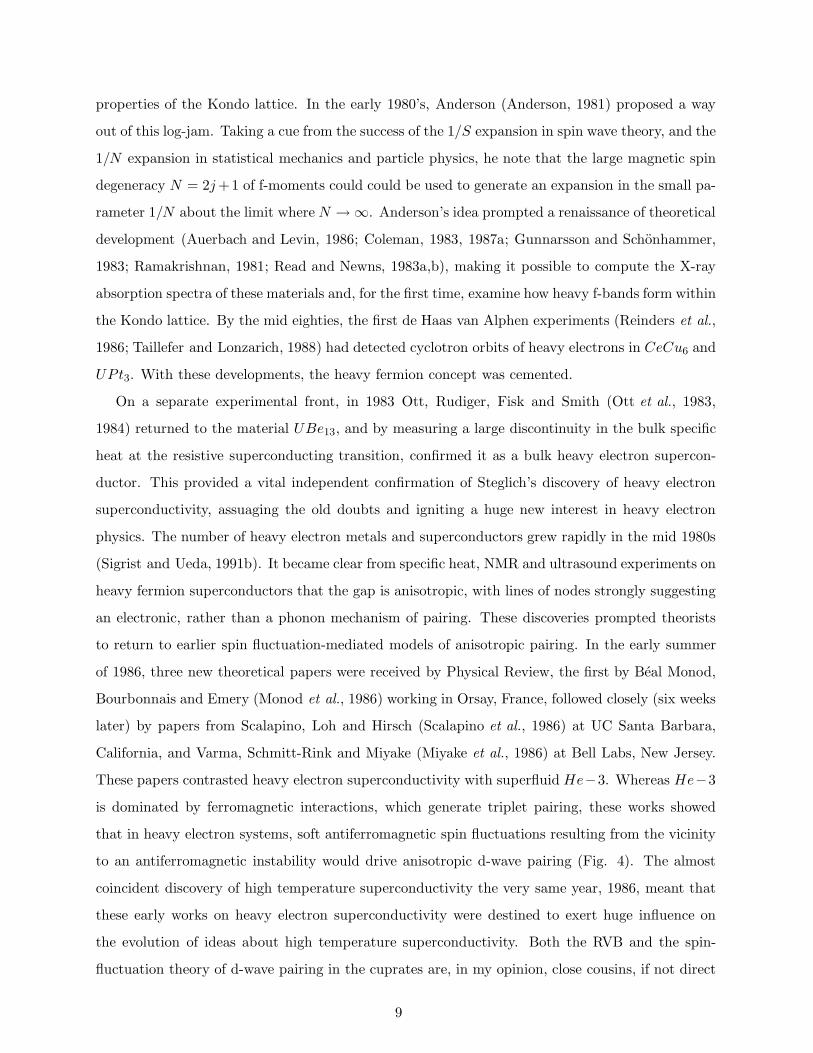
to an antiferromagnetic instability would drive anisotropic d-wave pairing (Fig. 4). The almost
coincident discovery of high temperature superconductivity the very same year, 1986, meant that
these early works on heavy electron superconductivity were destined to exert huge influence on
the evolution of ideas about high temperature superconductivity. Both the RVB and the spin-
fluctuation theory of d-wave pairing in the cuprates are, in my opinion, close cousins, if not direct
9
FIG. 4 Figure from (Monod et al., 1986), one of three path-breaking papers in 1986 to link d-wave pairing
to antiferromagnetism. (a) is the bare interaction, (b) and (c) and (d) the paramagnon mediated interaction
between anti-parallel or parallel spins.
descendents of these early 1986 papers on heavy electron superconductivity.
After a brief hiatus, interest in heavy electron physics re-ignited in the mid 1990’s with the
discovery of quantum critical points in these materials. High temperature superconductivity intro-
duced many important new ideas into our conception of electron fluids, including
• Non Fermi liquid behavior: the emergence of metallic states that can not be described as
fluids of renormalized quasiparticles.
• Quantum phase transitions and the notion that zero temperature quantum critical points
might profoundly modify finite temperature properties of metal.
Both of these effects are seen in a wide variety of heavy electron materials, providing an vital
alternative venue for research on these still unsolved aspects of interlinked, magnetic and electronic
behavior.
In 1995, Hilbert von Lohneyson and collaborators discovered that by alloying small amounts
of gold into CeCu6 that one can tune CeCu6−xAux through an antiferromagnetic quantum crit-
ical point, and then reverse the process by the application of pressure (von Lohneysen, 1996;
von Lohneysen et al., 1994). These experiments showed that a heavy electron metal develops “non-
Fermi liquid” properties at a quantum critical point, including a linear temperature dependence of
the resistivity and a logarithmic dependence of the specific heat coefficient on temperature. Shortly
thereafter, Mathur et al. (Mathur et al., 1998), at Cambridge showed that when pressure is used
10
to drive the antiferromagnet CeIn3 through through a quantum phase transition, heavy electron
superconductivity develops in the vicinity of the quantum phase transition. Many new examples
of heavy electron system have come to light in the last few years which follow the same pattern.
In one fascinating development, (Monthoux and Lonzarich, 1999) suggested that if quasi-two di-
mensional versions of the existing materials could be developed, then the superconducting pairing
would be less frustrated, leading to a higher transition temperature. This led experimental groups
to explore the effect of introducing layers into the material CeIn3, leading to the discovery of the
so called 1− 1− 5 compounds, in which an XIn2 layer has been introduced into the original cubic
compound. (Petrovic et al., 2001; Sidorov et al., 2002). Two notable members of this group are
CeCoIn5 and most recently, PuCoGa5 (Sarrao et al., 2002). The transition temperature rose from
0.5K to 2.5K in moving from CeIn3 to CeCoIn5. Most remarkably, the transition temperature
rises to above 18K in the PuCoGa5 material. This amazing rise in Tc, and its close connection with
quantum criticality, are very active areas of research, and may hold important clues (Curro et al.,
2005) to the ongoing quest to discover room temperature superconductivity.
B. Key elements of Heavy Fermion Metals
Before examining the theory of heavy electron materials, we make a brief tour of their key
properties. Table A. shows a selective list of heavy fermion compounds
1. Spin entropy: a driving force for new physics
The properties of heavy fermion compounds derive from the partially filled f orbitals of rare
earth or actinide ions (Fulde et al., 1988; Grewe and Steglich, 1991; Lee et al., 1986; Ott, 1987;
Stewart, 1984). The large nuclear charge in these ions causes their f orbitals to collapse inside the
inert gas core of the ion, turning them into localized magnetic moments.
11

Table. A. Selected Heavy Fermion Compounds.
TypeMaterial T ∗ Tc, xc, Bc Properties ρ γn
mJmol−1K−2
Ref.
Metal CeCu6 10K -Simple HF
MetalT 2 1600 [1]
Super-
conductors
CeCu2Si2 20K Tc=0.17K First HFSC T 2 800-1250 [2]
UBe13 2.5K Tc=0.86KIncoherent
metal→HFSC
ρc ∼150µΩcm
800 [3]
CeCoIn5 38K Tc=2.3K Quasi 2D HFSC T 750 [4]
Kondo
Insulators
Ce3Pt4Bi3 Tχ ∼ 80K -Fully Gapped
KI∼ e∆/T - [5]
CeNiSn Tχ ∼ 20K - Nodal KIPoor
Metal- [6]
Quantum
Critical
CeCu6−xAux T0 ∼ 10K xc = 0.1Chemically
tuned QCPT ∼ 1
T0ln
(T0
T
)[7]
Y bRh2Si2 T0 ∼ 24KB⊥=0.06T
B‖=0.66T
Field-tuned
QCPT ∼ 1
T0ln
(T0
T
)[8]
SC +
other
Order
UPd2Al3 110KTAF =14K,
Tsc=2KAFM + HFSC T 2 210 [9]
URu2Si2 75KT1=17.5K,
Tsc=1.3K
Hidden Order &
HFSCT 2 120/65 [10]
Unless otherwise stated, T ∗ denotes the temperature of the maximum in resistivity. Tc, xc and Bc
denote critical temperature, doping and field. ρ denotes the temperature temperature dependence in the
normal state.γn = CV /T is the specific heat coefficient in the normal state. [1] (Onuki and Komatsubara,
1987; Stewart et al., 1984b), [2] (Geibel et al., 1991; Geibel. et al., 1991; Steglich et al., 1976), [3] (Ott et al.,
1983, 1984), [4] (Petrovic et al., 2001; Sidorov et al., 2002), [5] (Bucher et al., 1994; Hundley et al., 1990), [6]
(Izawa et al., 1999; Takabatake et al., 1992, 1990), [7] (von Lohneysen, 1996; von Lohneysen et al., 1994), [8]
(Custers et al., 2003; Gegenwart et al., 2005; Paschen et al., 2004; Trovarelli et al., 2000), [9] (Geibel et al.,
12
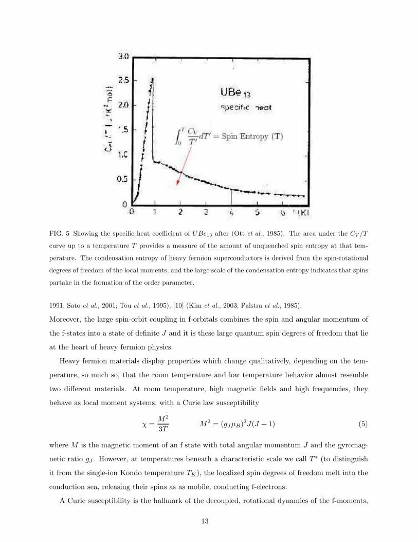
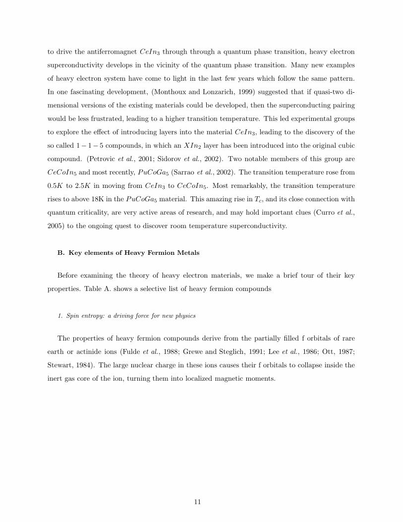
FIG. 5 Showing the specific heat coefficient of UBe13 after (Ott et al., 1985). The area under the CV /T
curve up to a temperature T provides a measure of the amount of unquenched spin entropy at that tem-
perature. The condensation entropy of heavy fermion superconductors is derived from the spin-rotational
degrees of freedom of the local moments, and the large scale of the condensation entropy indicates that spins
partake in the formation of the order parameter.
1991; Sato et al., 2001; Tou et al., 1995), [10] (Kim et al., 2003; Palstra et al., 1985).
Moreover, the large spin-orbit coupling in f-orbitals combines the spin and angular momentum of
the f-states into a state of definite J and it is these large quantum spin degrees of freedom that lie
at the heart of heavy fermion physics.
Heavy fermion materials display properties which change qualitatively, depending on the tem-
perature, so much so, that the room temperature and low temperature behavior almost resemble
two different materials. At room temperature, high magnetic fields and high frequencies, they
behave as local moment systems, with a Curie law susceptibility
χ =M2
3TM2 = (gJµB)2J(J + 1) (5)
where M is the magnetic moment of an f state with total angular momentum J and the gyromag-
netic ratio gJ . However, at temperatures beneath a characteristic scale we call T ∗ (to distinguish
it from the single-ion Kondo temperature TK), the localized spin degrees of freedom melt into the
conduction sea, releasing their spins as as mobile, conducting f-electrons.
A Curie susceptibility is the hallmark of the decoupled, rotational dynamics of the f-moments,
13

associated with an unquenched entropy of S = kB lnN per spin, where N = 2J + 1 is the spin-
degeneracy of an isolated magnetic moment of angular momentum J . For example, in a Cerium
heavy electron material, the 4f1 (L = 3) configuration of the Ce3+ ion is spin-orbit coupled into a
state of definite J = L− S = 5/2 with N = 6. Inside the crystal, the full rotational symmetry of
each magnetic f-ion is often reduced by crystal fields to a quartet (N = 4) or a Kramer’s doublet
N = 2. At the characteristic temperature T ∗, as the Kondo effect develops, the spin entropy is
rapidly lost from the material, and large quantities of heat are lost from the material. Since the
area under the specific heat curve determines the entropy,
S(T ) =
∫ T
0
CVT ′ dT
′, (6)
a rapid loss of spin entropy at low temperatures forces a sudden rise in the specific heat capacity.
Fig. 5 illustrates this phenomenon with the specific heat capacity of UBe13. Notice how the specific
heat coefficient CV /T rises to a value of order 1J/mol/K2, and starts to saturate at about 1K,
indicating the formation of a Fermi liquid with a linear specific heat coefficient. Remarkably, just
as the linear specific heat starts to develop, UBe13 becomes superconducting, as indicated by the
large specific heat anomaly.
2. “Local” Fermi liquids with a single scale
The standard theoretical framework for describing metals is Landau Fermi liquid theory
(Landau, 1957), according to which, the excitation spectrum of a metal can be adiabatically con-
nected to those of a non-interacting electron fluid. Heavy Fermion metals are extreme examples of
Landau Fermi liquids which push the idea of adiabaticity into an regime where the bare electron
interactions, on the scale of electron volts, are hundreds, even thousands of times larger than the
millivolt Fermi energy scale of the heavy electron quasiparticles. The Landau Fermi liquid that
develops in these materials shares much in common with the Fermi liquid that develops around an
isolated magnetic impurity (Nozieres, 1976; Nozieres and Blandin, 1980), once it is quenched by
the conduction sea as part of the Kondo effect. There are three key features of this Fermi liquid:
• Single scale T ∗ The quasiparticle density of states ρ∗ ∼ 1/T ∗ and scattering amplitudes
Akσ,k′σ′ ∼ T ∗ scale approximately with a single scale T ∗.
• Almost incompressible. Heavy electron fluids are “almost incompressible”, in the sense
that the charge susceptibility χc = dNe/dµ << ρ∗ is unrenormalized and typically more
14

than an order magnitude smaller than the quasiparticle density of states ρ∗. This is because
the lattice of spins severely modifies the quasiparticle density of states, but leaves the charge
density of the fluid ne(µ), and its dependence on the chemical potential µ unchanged.
• Local. Quasiparticles scatter when in the vicinity of a local moment, giving rise to a small
momentum dependence to the Landau scattering amplitudes. (Engelbrecht and Bedell, 1995;
Yamada, 1975; Yoshida and Yamada, 1975) .
Landau Fermi liquid theory relates the properties of a Fermi liquid to the density of states of the
quasiparticles and a small number of interaction parameters (Baym and Pethick, 1992) If Ekσ is
the energy of an isolated quasiparticle, then the quasiparticle density of states ρ∗ =∑
kσ δ(Ekσ−µ)
determines the linear specific heat coefficient
γ = LimT→0
(CVT
)
=π2k2
B
3ρ∗. (7)
In conventional metals the linear specific heat coefficient is of order 1 − 10 mJ mol−1K−2. In a
system with quadratic dispersion, Ek = h2k2
2m∗ , the quasiparticle density of states and effective mass
m∗ are directly proportional
ρ∗ =
(kF
π2h2
)
m∗, (8)
where kF is the Fermi momentum. In heavy fermion compounds, the scale of ρ∗ varies widely,
and specific heat coefficients in the range 100 − 1600 mJ mol−1K−2 have been observed. From
this simplified perspective, the quasiparticle effective masses in heavy electron materials are two
or three orders of magnitude “heavier” than in conventional metals.
In Landau Fermi liquid theory, a change δnk′σ′ in the quasiparticle occupancies causes a shift
in the quasiparticle energies given by
δEkσ =∑
k′σ′
fkσ,kσ′δnk′σ′ (9)
In a simplified model with a spherical Fermi surface, the Landau interaction parameters only
depend on the relative angle θk,k′ between the quasiparticle momenta, and are expanded in terms
of Legendre Polynomials as
fkσ,kσ′ =1
ρ∗∑
l
(2l + 1)Pl(θk,k′)[F sl + σσ′F al ]. (10)
The dimensionless “Landau parameters” F s,al parameterize the detailed quasiparticle interactions.
The s-wave (l = 0) Landau parameters determine the magnetic and charge susceptibility of a
15
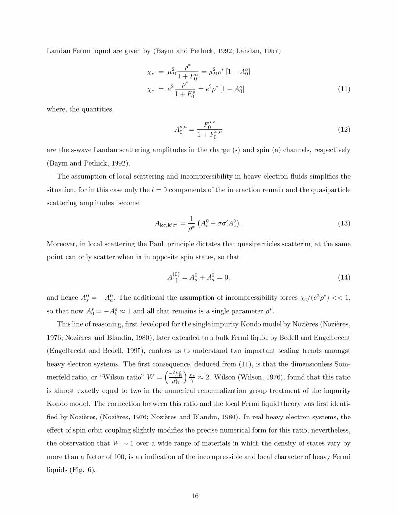
Landau Fermi liquid are given by (Baym and Pethick, 1992; Landau, 1957)
χs = µ2B
ρ∗
1 + F a0= µ2
Bρ∗ [1 −Aa0]
χc = e2ρ∗
1 + F s0= e2ρ∗ [1 −As0] (11)
where, the quantities
As,a0 =F s,a0
1 + F s,a0
(12)
are the s-wave Landau scattering amplitudes in the charge (s) and spin (a) channels, respectively
(Baym and Pethick, 1992).
The assumption of local scattering and incompressibility in heavy electron fluids simplifies the
situation, for in this case only the l = 0 components of the interaction remain and the quasiparticle
scattering amplitudes become
Akσ,k′σ′ =1
ρ∗(A0s + σσ′A0
a
). (13)
Moreover, in local scattering the Pauli principle dictates that quasiparticles scattering at the same
point can only scatter when in in opposite spin states, so that
A(0)↑↑ = A0
s +A0a = 0. (14)
and hence A0s = −A0
a. The additional the assumption of incompressibility forces χc/(e2ρ∗) << 1,
so that now As0 = −Aa0 ≈ 1 and all that remains is a single parameter ρ∗.
This line of reasoning, first developed for the single impurity Kondo model by Nozieres (Nozieres,
1976; Nozieres and Blandin, 1980), later extended to a bulk Fermi liquid by Bedell and Engelbrecht
(Engelbrecht and Bedell, 1995), enables us to understand two important scaling trends amongst
heavy electron systems. The first consequence, deduced from (11), is that the dimensionless Som-
merfeld ratio, or “Wilson ratio” W =(π2k2
B
µ2B
)χs
γ ≈ 2. Wilson (Wilson, 1976), found that this ratio
is almost exactly equal to two in the numerical renormalization group treatment of the impurity
Kondo model. The connection between this ratio and the local Fermi liquid theory was first identi-
fied by Nozieres, (Nozieres, 1976; Nozieres and Blandin, 1980). In real heavy electron systems, the
effect of spin orbit coupling slightly modifies the precise numerical form for this ratio, nevertheless,
the observation that W ∼ 1 over a wide range of materials in which the density of states vary by
more than a factor of 100, is an indication of the incompressible and local character of heavy Fermi
liquids (Fig. 6).
16

FIG. 6 Plot of linear specific heat coefficient vs Pauli susceptibility to show approximate constancy of Wilson
ratio. (After B. Jones (Lee et al., 1986)).
A second consequence of locality appears in the transport properties. In a Landau Fermi liquid,
inelastic electron-electron scattering produces a quadratic temperature dependence in the resistivity
ρ(T ) = ρ0 +AT 2. (15)
In conventional metals, resistivity is dominated by electron-phonon scattering, and the “A” coeffi-
cient is generally too small for the electron-electron contribution to the resistivity to be observed.
In strongly interacting metals, the A coefficient becomes large, and in a beautiful piece of phe-
nomenology, Kadowaki and Woods (Kadowaki and Woods, 1986), observed that the ratio of A to
the square of the specific heat coefficient γ2
αKW =A
γ2≈ (1 × 10⁻⁵)µΩcm[mol K2/mJ] (16)
is approximately constant, over a range of A spanning four orders of magnitude. This too, can be
simply understood from local Fermi liquid theory, where the local scattering amplitudes give rise
to an electron mean-free path given by
1
kF l∗∼ constant +
T 2
(T ∗)2. (17)
The “A” coefficient in the electron resistivity that results from the second-term satisfies A ∝1
(T ∗)2∝ γ2. A more detailed calculation is able to account for the magnitude of the Kadowaki
17

FIG. 7 Approximate constancy of the Kadowaki Woods ratio, for a wide range of heavy electrons, after
(Tsujji et al., 2005). When spin-orbit effects are taken into account, the Kadowaki Wood ratio depends on
the effective degeneracy N = 2J +1 of the magnetic ion, which when taken into account leads to a far more
precise collapse of the data onto a single curve.
Woods constant, and its weak residual dependence on the spin degeneracy N = 2J + 1 of the
magnetic ions (see Fig. 7.).
The approximate validity of the scaling relations
χ
γ≈ cons,
A
γ2≈ cons (18)
for a wide range of heavy electron compounds, constitutes excellent support for the Fermi liquid
picture of heavy electrons.
A classic signature of heavy fermion behavior is the dramatic change in transport properties
that accompanies the development of a coherent heavy fermion band structure(Fig. [6]). At high
temperatures heavy fermion compounds exhibit a large saturated resistivity, induced by incoherent
spin-flip scattering of the conduction electrons off the local f-moments. This scattering grows as the
temperature is lowered, but at the same time, it becomes increasingly elastic at low temperatures.
18

FIG. 8 Development of coherence in in Ce1−xLaxCu6 after Onuki and Komatsubara
(Onuki and Komatsubara, 1987).
This leads to the development of phase coherence. the f-electron spins. In the case of heavy fermion
metals, the development of coherence is marked by a rapid reduction in the resistivity, but in a
remarkable class of heavy fermion or “Kondo insulators”, the development of coherence leads to a
filled band with a tiny insulating gap of order TK . In this case coherence is marked by a sudden
exponential rise in the resistivity and Hall constant.
The classic example of coherence is provided by metallic CeCu6, which develops “coherence”
and a maximum in its resistivity around T = 10 K. Coherent heavy electron propagation is readily
destroyed by substitutional impurities. In CeCu6, Ce3+ ions can be continuously substituted with
non magnetic La3+ ions, producing a continuous cross-over from coherent Kondo lattice to single
impurity behavior (Fig. 8 ).
One of the important principles of the Landau Fermi liquid is the Fermi surface counting rule,
or Luttinger’s theorem(Luttinger, 1960). In non interacting electron band theory, the volume of
the Fermi surface counts the number of conduction electrons. For interacting systems this rule
survives (Martin, 1982; Oshikawa, 2000), with the unexpected corollary that the spin states of the
screened local moments are also included in the sum
2VFS
(2π)3= [ne + nspins] (19)
Remarkably, even though f-electrons are localized as magnetic moments at high temperatures, in
the heavy Fermi liquid, they contribute to the Fermi surface volume.
The most most direct evidence for the large heavy f- Fermi surfaces derives from de Haas
van Alphen and Shubnikov de Haas experiments that measure the oscillatory diamagnetism or
and resistivity produced by coherent quasiparticle orbits (Fig. 9). These experiments provide
a direct measure of the heavy electron mass, the Fermi surface geometry and volume. Since the
19

FIG. 9 (a) Fermi surface of UPt3 calculated from band-theory assuming itinerant 5f electrons
(Norman et al., 1988; Oguchi and Freeman, 1985; Wang et al., 1987), showing three orbits (σ, ω and τ)
that are identified by dHvA measurements, after (Kimura et al., 1998). (b) Fourier transform of dHvA
oscillations identifying σ, ω and τ orbits shown in (a).
pioneering measurements on CeCu6 and UPt3 by Reinders and Springford, Taillefer and Lonzarich
in the mid-eighties (Reinders et al., 1986; Taillefer and Lonzarich, 1988; Taillefer et al., 1987), an
extensive number of such measurements have been carried out (Julian et al., 1992; Kimura et al.,
1998; McCollam et al., 2005; Onuki and Komatsubara, 1987). Two key features are observed:
• A Fermi surface volume which counts the f-electrons as itinerant quasiparticles.
• Effective masses often in excess of one hundred free electron masses. Higher mass quasi-
particle orbits, though inferred from thermodynamics, can not be observed with current
measurement techniques.
• Often, but not always, the Fermi surface geometry is in accord with band-theory, despite
the huge renormalizations of the electron mass.
Additional confirmation of the itinerant nature of the f-quasiparticles comes from the observa-
tion of a Drude peak in the optical conductivity. At low temperatures, in the coherent regime,
an extremely narrow Drude peak can be observed in the optical conductivity of heavy fermion
metals. The weight under the Drude peak is a measure of the plasma frequency: the diamagnetic
response of the heavy fermion metal. This is found to be extremely small, depressed by the large
mass enhancement of the quasiparticles (DeGiorgi, 1999; Millis et al., 1987a).∫
|ω|<g
TK
dω
πσqp(ω) =
ne2
m∗ (6)
Both the optical and dHvA experiments indicate that the presence of f-spins depresses both the
spin and diamagnetic response of the electron gas down to low temperatures.
20

II. LOCAL MOMENTS AND THE KONDO LATTICE
A. Local Moment Formation
1. The Anderson Model
We begin with a discussion of how magnetic moments form at high temperatures, and how they
are screened again at low temperatures to form a Fermi liquid. The basic model for local moment
formation is the Anderson model (Anderson, 1961)
H =
Hresonance︷ ︸︸ ︷∑
k,σ
ǫknkσ +∑
k,σ
V (k)[
c†kσfσ + f †σckσ]
+Efnf + Unf↑nf↓︸ ︷︷ ︸
Hatomic
(20)
where Hatomic describes the atomic limit of an isolated magnetic ion and Hresonance describes the
hybridization of the localized f-electrons in the ion with the Bloch waves of the conduction sea. For
pedagogical reasons, our discussion will initially focus on the case where the f-state is a Kramer’s
doublet.
There are two key elements to the Anderson model:
• Atomic limit. The atomic physics of an isolated ion with a single f state, described by the
model
Hatomic = Efnf + Unf↑nf↓. (21)
Here Ef is the energy of the f state and U is the Coulomb energy associated with two
electrons in the same orbital. The atomic physics contains the basic mechanism for local
moment formation, valid for f-electrons, but also seen in a variety of other contexts, such as
transition metal atoms and quantum dots.
The four quantum states of the atomic model are
|f2〉|f0〉
E(f2) = 2Ef + U
E(f0) = 0
non-magnetic
|f1 ↑〉, |f1 ↓〉 E(f1) = Ef . magnetic.
(22)
In a magnetic ground-state, the cost of inducing a “valence fluctuation” by removing or
adding an electron to the f1 state is positive, i.e.
removing: E(f0) − E(f1) = −Ef > 0 ⇒ U/2 > Ef + U/2,
21

FIG. 10 Phase diagram for Anderson Impurity Model in the Atomic Limit.
adding: E(f2) − E(f1) = Ed + U > 0 ⇒ Ed + U/2 > −U/2, (23)
or (Fig. 10).
U/2 > Ed + U/2 > −U/2. (24)
Under these conditions, a local moment is well-defined provided the temperature is smaller
than the valence fluctuation scale TV F = max(Ef + U,−Ef ). At lower temperatures, the
atom behaves exclusively as a quantum top.
• Virtual bound-state formation. When the magnetic ion is immersed in a sea of electrons,
the f-electrons within the core of the atom hybridize with the Bloch states of surrounding
electron sea (Blandin and Friedel, 1958) to form a resonance described by
Hresonance =∑
k,σ
ǫknkσ +∑
k,σ
[
V (k)c†kσfσ + V (k)∗f †σckσ]
(25)
where the hybridization matrix element V (k) = 〈k|Vatomic|f〉 is the overlap of the atomic
potential between a localized f-state and a Bloch wave. In the absence of any interactions,
the hybridization broadens the localized f-state, producing a resonance of width
∆ = π∑
k
|V (k)|2δ(ǫk − µ) = πV 2ρ (26)
where V 2 is the average of the hybridization around the Fermi surface.
There are two complimentary ways to approach the physics of the Anderson model
- the “atomic picture”, which starts with the interacting, but isolated atom (V (k) = 0), and
considers the effect of immersing it in an electron sea by slowly dialing up the hybridization.
22

- the “adiabatic picture” which starts with the non-interacting resonant ground-state (U = 0),
and then considers the effect of dialing up the interaction term U .
These approaches paint a contrasting and, at first sight, contradictory picture of a local moment in
a Fermi sea. From the adiabatic perspective, the ground-state is always a Fermi liquid (see I.B.2),
but from atomic perspective, provided the hybridization is smaller than U one expects a local
magnetic moment, whose low lying degrees of freedom are purely rotational. How do we resolve
this paradox?
Anderson’s original work provided a mean-field treatment of the interaction. He found that
at interactions larger than Uc ∼ π∆ local moments develop with a finite magnetization M =
〈n↑〉 − 〈n↓〉. The mean field theory provides an approximate guide to the conditions required
for moment formation, but it doesn’t account for the restoration of the singlet symmetry of the
ground-state at low temperatures. The resolution of the adiabatic and the atomic picture derives
from quantum spin fluctuations which cause the local moment to “tunnel” on a slow time-scale τsf
between the two degenerate “up” and “down” configurations.
e−↓ + f1↑ e−↑ + f1
↓ (27)
These fluctuations are the origin of the Kondo effect. From the energy uncertainty principle,
below a temperature TK at which the thermal excitation energy kBT is of order the characteristic
tunneling rate hτsf
, a paramagnetic state with a Fermi liquid resonance will form. The characteristic
width of the resonance is then determined by the Kondo energy kBTK ∼ hτsf
. The existence of
this resonance was first deduced by Abrikosov and Suhl (Abrikosov, 1965; Suhl, 1965), but it is
more frequently called the “Kondo resonance”. From perturbative renormalization group reasoning
(D and Haldane, 1978)and the Bethe ansatz solution of the Anderson model (Okiji and Kawakami,
1983; Wiegmann, 1980a,b) we know that for large U >> ∆, the Kondo scale depends exponentially
on U . In the symmetric Anderson model, where Ef = −U/2,
TK =
√
2U∆
π2exp
(
−πU8∆
)
. (28)
The temperature TK marks the crossover from a a high temperature Curie law χ ∼ 1T susceptibility
to a low temperature paramagnetic susceptibility χ ∼ 1/TK .
23

2. Adiabaticity and the Kondo resonance
A central quantity in the physics of f-electron systems is the f-spectral function,
Af (ω) =1
πImGf (ω − iδ) (29)
where Gf (ω) = −i∫ ∞−∞ dt〈Tfσ(t)f †σ(0)〉eiωt is the Fourier transform of the time-ordered f-Green’s
function. When an f-electron is added, or removed from the f-state, the final state has a distribution
of energies described by the f-spectral function. From a spectral decomposition of the f-Green’s
function, the positive energy part of the f-spectral function determines the energy distribution for
electron addition, while the negative energy part measures the energy distribution of for electron
removal:
Af (ω) =
Energy distribution of state formed by adding one f-electron.︷ ︸︸ ︷∑
λ
∣∣∣〈λ|f †σ|φ0〉
∣∣∣
2δ(ω − [Eλ − E0]), (ω > 0)
∑
λ
|〈λ|fσ|φ0〉|2 δ(ω − [E0 − Eλ]),
︸ ︷︷ ︸
Energy distribution of state formed by removing an f-electron
(ω < 0)(30)
where E0 is the energy of the ground-state, and Eλ is the energy of an excited state λ, formed
by adding or removing an f-electron. For negative energies, this spectrum can be measured by
measuring the energy distribution of photo-electrons produced by X-ray photo-emission, while
for positive energies, the spectral function can be measured from inverse X-ray photo-emission
(Allen et al., 1986, 1983). The weight beneath the Fermi energy peak, determines the f-charge of
the ion
〈nf 〉 = 2
∫ 0
−∞dωAf (ω) (31)
In a magnetic ion, such as a Cerium atom in a 4f1 state, this quantity is just a little below unity.
Fig. (11.) illustrates the effect of the interaction on the f-spectral function. In the non-
interacting limit (U = 0), the f-spectral function is a Lorentzian of width ∆. If we turn on the
interaction U , being careful to shifting the f-level position beneath the Fermi energy to maintain
a constant occupancy, the resonance splits into three peaks, two at energies ω = Ef and ω =
Ef +U corresponding to the energies for a valence fluctuation, plus an additional central “Kondo
resonance” associated with the spin-fluctuations of the local moment.
At first sight, once the interaction is much larger than the hybridization width ∆, one might
expect there to be no spectral weight left at low energies. But this violates the idea of adiabaticity.
In fact, there are always certain adiabatic invariants that do not change, despite the interaction.
24

FIG. 11 Schematic illustrating the evaluation of the f-spectral function Af (ω) as interaction strength U is
turned on continuously, maintaining a constant f-occupancy by shifting the bare f-level position beneath
the Fermi energy. The lower part of diagram is the density plot of f-spectral function, showing how the
non-interacting resonance at U = 0 splits into an upper and lower atomic peak at ω = Ef and ω = Ef +U .
One such quantity is the phase shift δf associated with the scattering of conduction electrons off
the ion; another is the height of the f-spectral function at zero energy, and it turns out that these
two quantities are related. A rigorous result due to Langreth (Langreth, 1966), tells us that the
spectral function at ω = 0 is diretly determined by the f-phase shift, so that its non-interacting
25

value
Af (ω = 0) =sin2 δfπ∆
, (32)
is preserved by adiabaticity. Langreth’s result can be heuristically derived by noting that δf is the
phase of the f-Green’s function at the Fermi energy, so that Gf (0− iδ)−1 = ‖G−1f (0)|e−iδf . Now in
a Fermi liquid, the scattering at the Fermi energy is purely elastic, and this implies that ImG−1f (0−
iδ) = ∆, the bare hybridization width. From this it follows that ImG−1f (0) = |G−1
f (0)| sin δf = ∆,
so that Gf (0) = eiδf /(∆ sin δ), and the above result follows.
The phase shift δf is set via the Friedel sum rule, according to which the sum of the up and
down scattering phase shifts, gives the total number of f-bound-electrons, or
∑
σ
δfσπ
= 2δfπ
= nf . (33)
for a two-fold degenerate f− state. At large distances, the wavefunction of scattered electrons
ψf (r) ∼ sin(kF r + δf )/r is “shifted inwards” by by a distance δl/kF = (λF /2) × (δl/π). This
sum rule is sometimes called a “node counting” rule, because if you think about a large sphere
enclosing the impurity, then each time the phase shift passes through π, a node crosses the spherical
boundary and one more electron per channel is bound beneath the Fermi sea. Friedel’s sum rule
holds for interacting electrons, providing the ground-state is adiabatically accessible from the non-
interacting system (Langer and Ambegaokar, 1961; Langreth, 1966). Since nf = 1 in an f1 state,
the Friedel sum rule tells us that the phase shift is π/2 for a two-fold degenerate f− state. In other
words, adiabaticity tell us that the electron is resonantly scattered by the quenched local moment.
Photo-emission studies do reveal the three-peaked structure characteristic of the Anderson
model in many Ce systems, such as CeIr2 and CeRu2 (Allen et al., 1983) (see Fig. 12). Ma-
terials in which the Kondo resonance is wide enough to be resolved are more “mixed valent”
materials in which the f- valence departs significantly from unity. Three peaked structures have
also been observed in certain U 5f materials such as UPt3 and UAl2 (Allen et al., 1985)materials,
but it has not yet been resolved in UBe13. A three peaked structure has recently been observed
in 4f Y b materials, such as Y bPd3, where the 4f13 configuration contains a single f hole, so that
the positions of the three peaks are reversed relative to Ce (Liu et al., 1992).
26

FIG. 12 Showing spectral functions for three different Cerium f-electron materials, measured using X-ray
photoemission (below the Fermi energy ) and inverse X-ray photoemission (above the Fermi energy) after
(Allen et al., 1983). CeAl is an antiferromagnet and does not display a Kondo resonance.
B. Hierachies of energy scales
1. Renormalization Concept
To understand how a Fermi liquid emerges when a local moment is immersed in a quantum sea of
electrons, theorists had to connect physics on on several widely spaced energy scales. Photoemission
shows that the characteristic energy to produce a valence fluctuation is of the order of volts, or
tens of thousands of Kelvin, yet the the characteristic physics we are interested in occurs at scales
hundreds, or thousands of times smaller. How can we distill the essential effects of the atomic
physics at electron volt scales on the low energy physics at millivolt scales?
The essential tool for this task is the “renormalization group” (Anderson, 1970, 1973;
Anderson and Yuval, 1969, 1970, 1971; Nozieres, 1976; Nozieres and Blandin, 1980; Wilson, 1976),
based on the idea that the physics at low energy scales only depends on a small subset of “relevant”
27

FIG. 13 (a) Cross-over energy scales for the Anderson model. At scales below ΛI , valence fluctuations into
the doubly occupied state are suppressed. All lower energy physics is described by the infinite U Anderson
model. Below ΛII , all valence fluctuations are suppressed, and the physics involves purely the spin degrees of
freedom of the ion, coupled to the conduction sea via the Kondo interaction. The Kondo scale renormalizes
to strong coupling below ΛIII , and the local moment becomes screened to form a local Fermi liquid. (b)
Illustrating the idea of renormalization group flows towards a Fermi liquid fixed point.
variables from the original microscopic Hamiltonian. The extraction of these relevant variables is
accomplished by “renormalizing” the Hamiltonian by systematically eliminating the high energy
virtual excitations and adjusting the low energy Hamiltonian to take care of the interactions that
these virtual excitations induce in the low energy Hilbert space. This leads to a family of Hamilto-
nian’s H(Λ), each with a different high-energy cut-off Λ, which share the same low energy physics.
The systematic passage from a Hamiltonian H(Λ) to a renormalized Hamiltonian H(Λ′) with
a smaller cutoff Λ′ = Λ/b is accomplished by dividing the the eigenstates of H into a a low energy
subspace L and a high energy subspace H, with energies |ǫ| < Λ′ = Λ/b and a |ǫ| ∈ [Λ′,Λ]
respectively. The Hamiltonian is then broken up into terms that are block-diagonal in these
subspaces,
H =
[HL
V
∣∣∣∣
V †
HH
]
, (34)
where V and V † provide the matrix elements between L and H. The effects of the V are then
taken into account by carrying out a unitary (canonical) transformation that block-diagonalizes
the Hamiltonian,
H(Λ) → UH(Λ)U † =
[
HL
0
∣∣∣∣∣
0
HH
]
(35)
28
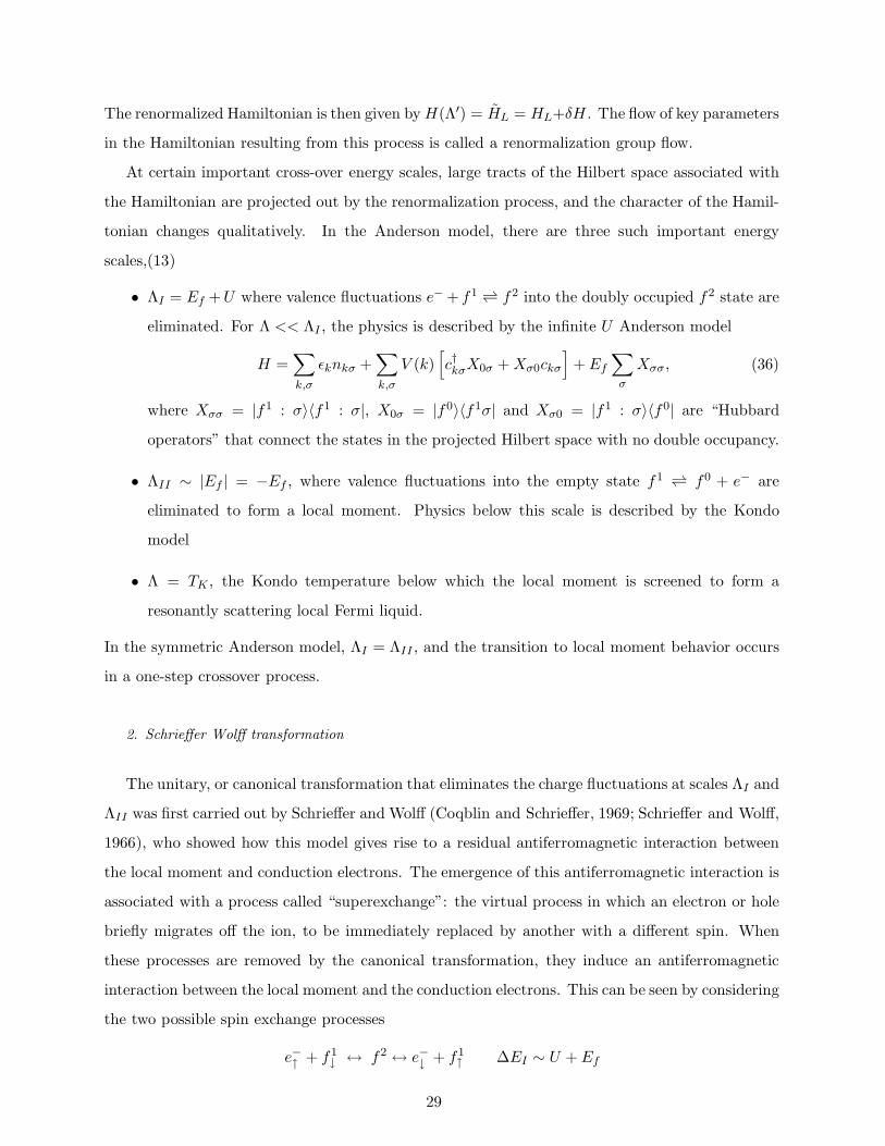
The renormalized Hamiltonian is then given byH(Λ′) = HL = HL+δH . The flow of key parameters
in the Hamiltonian resulting from this process is called a renormalization group flow.
At certain important cross-over energy scales, large tracts of the Hilbert space associated with
the Hamiltonian are projected out by the renormalization process, and the character of the Hamil-
tonian changes qualitatively. In the Anderson model, there are three such important energy
scales,(13)
• ΛI = Ef +U where valence fluctuations e− + f1 f2 into the doubly occupied f2 state are
eliminated. For Λ << ΛI , the physics is described by the infinite U Anderson model
H =∑
k,σ
ǫknkσ +∑
k,σ
V (k)[
c†kσX0σ +Xσ0ckσ
]
+ Ef∑
σ
Xσσ , (36)
where Xσσ = |f1 : σ〉〈f1 : σ|, X0σ = |f0〉〈f1σ| and Xσ0 = |f1 : σ〉〈f0| are “Hubbard
operators” that connect the states in the projected Hilbert space with no double occupancy.
• ΛII ∼ |Ef | = −Ef , where valence fluctuations into the empty state f1 f0 + e− are
eliminated to form a local moment. Physics below this scale is described by the Kondo
model
• Λ = TK , the Kondo temperature below which the local moment is screened to form a
resonantly scattering local Fermi liquid.
In the symmetric Anderson model, ΛI = ΛII , and the transition to local moment behavior occurs
in a one-step crossover process.
2. Schrieffer Wolff transformation
The unitary, or canonical transformation that eliminates the charge fluctuations at scales ΛI and
ΛII was first carried out by Schrieffer and Wolff (Coqblin and Schrieffer, 1969; Schrieffer and Wolff,
1966), who showed how this model gives rise to a residual antiferromagnetic interaction between
the local moment and conduction electrons. The emergence of this antiferromagnetic interaction is
associated with a process called “superexchange”: the virtual process in which an electron or hole
briefly migrates off the ion, to be immediately replaced by another with a different spin. When
these processes are removed by the canonical transformation, they induce an antiferromagnetic
interaction between the local moment and the conduction electrons. This can be seen by considering
the two possible spin exchange processes
e−↑ + f1↓ ↔ f2 ↔ e−↓ + f1
↑ ∆EI ∼ U + Ef
29

h+↑ + f1
↓ ↔ f0 ↔ h+↓ + f1
↑ ∆EII ∼ −Ef (37)
Both process requires that the f-electron and incoming particle are in a spin-singlet. From second
order perturbation theory, the energy of the singlet is lowered by an amount −2J where
J = V 2
[1
∆E1+
1
∆E2
]
, (38)
and the factor of two derives from the two ways a singlet can emit an electron or hole into the
continuum 1 and V ∼ V (kF ) is the hybridization matrix element near the Fermi surface. For the
symmetric Anderson model, where ∆E1 = ∆EII = U/2, J = 4V 2/U .
If we introduce the electron spin density operator ~σ(0) = 1N
∑
k,k′ c†kα~σαβck′β, where N is the
number of sites in the lattice, then the effective interaction will have the form
HK = −2JPS=0 (39)
where PS=0 =[
14 − 1
2~σ(0) · ~Sf]
is the singlet projection operator. If we drop the constant term,
then the effective interaction induced by the virtual charge fluctuations must have the form
HK = J~σ(0) · ~Sf (40)
where ~Sf is the spin of the localized moment. The complete “Kondo Model”, H = Hc + HK
describing the conduction electrons and their interaction with the local moment is
H =∑
kσ
ǫkc†~kσc~kσ + J~σ(0) · ~Sf . (41)
3. The Kondo Effect
The anti-ferromagnetic sign of the super-exchange interaction J in the Kondo Hamiltonian is
the origin of the spin screening physics of the Kondo effect. The bare interaction is weak, but
the spin fluctuations it induces have the effect of antiscreening the interaction at low energies,
renormalizing it to larger and larger values. To see this, we follow a Anderson’s “Poor Man’s”
scaling procedure (Anderson, 1970, 1973), which takes advantage of the observation that at small
1 To calculate the matrix elements associated with valence fluctuations, take
|f1c1〉 =1√2(f†
↑c†↓ − c†↑f†↓ )|0〉, |f2〉 = f†
↑f†↓ |0〉 and |c2〉 = c†↑c
†↓|0〉
then 〈c2|P
σ V c†σfσ|f1c1〉 =√
2V and 〈f2|P
σ V f†σcσ|f1c1〉 =
√2V
30

J the renormalization in the Hamiltonian associated with the block-diagonalization process δH =
HL −HL is given by second-order perturbation theory:
δHab = 〈a|δH|b〉 =1
2[Tab(Ea) + Tab(Eb)] (42)
where
Tab(ω) =∑
|Λ〉∈H
[
V †aΛVΛb
ω − EΛ
]
(43)
is the many body “t-matrix” associated with virtual transitions into the high-energy subspace H.For the Kondo model,
V = PHJ ~S(0) · ~SdPL (44)
where PH projects the intermediate state into the high energy subspace while PL projects the initial
state into the low energy subspace. There are two virtual scattering processes that contribute the
the antiscreening effect, involving a high energy electron (I) or a high energy hole (II).
Process I is denoted by the diagram
and starts in state |b〉 = |kα, σ〉 , passes through a virtual state |Λ〉 = |c†k′′ασ′′〉 where ǫk′′ lies at high
energies in the range ǫk′′ ∈ [Λ/b,Λ] and ends in state |a〉 = |k′β, σ′〉. The resulting renormalization
〈k′β, σ′|T I(E)|kα, σ〉 = =∑
ǫk′′∈[Λ−δΛ,Λ]
[1
E − ǫk′′
]
J2 × (σaβλσbλα)(S
aσ′σ′′S
bσ′′σ)
≈ J2ρδΛ
[1
E − Λ
]
(σaσb)βα(SaSb)σ′σ (45)
In Process II, denoted by
the formation of a virtual hole excitation |Λ〉 = ck′′λ|σ′′〉 introduces an electron line that crosses
itself, introducing a negative sign into the scattering amplitude. The spin operators of the conduc-
tion sea and antiferromagnet reverse their relative order in process II, which introduces a relative
31

minus sign into the T-matrix for scattering into a high-energy hole-state,
〈k′βσ′|T (II)(E)|kασ〉 = −∑
ǫk′′∈[−Λ,−Λ+δΛ]
[1
E − (ǫk + ǫk′ − ǫk′′)
]
J2(σbσa)βα(SaSb)σ′σ
= −J2ρδΛ
[1
E − Λ
]
(σaσb)βα(SaSb)σ′σ (46)
where we have assumed that the energies ǫk and ǫk′ are negligible compared with Λ.
Adding (Eq. 45) and (Eq. 46) gives
δH intk′βσ′;kασ = T I + T II = −J
2ρδΛ
Λ[σa, σb]βαS
aSb
= 2J2ρδΛ
Λ~σβα~Sσ′σ. (47)
so the high energy virtual spin fluctuations enhance or “anti-screen” the Kondo coupling constant
J(Λ′) = J(Λ) + 2J2ρδΛ
Λ(48)
If we introduce the coupling constant g = ρJ , recognizing that d ln Λ = − δΛΛ we see that it satisfies
∂g
∂ ln Λ= β(g) = −2g2 +O(g3). (49)
This is an example of a negative β function: a signature of an interaction which grows with
the renormalization process. At high energies, the weakly coupled local moment is said to be
asymptotically free. The solution to the scaling equation is
g(Λ′) =go
1 − 2go ln(Λ/Λ′)(50)
and if we introduce the “Kondo temperature”
TK = D exp
[
− 1
2go
]
(51)
we see that this can be written
2g(Λ′) =1
ln(Λ/TK)(52)
so that once Λ′ ∼ TK , the coupling constant becomes of order one - at lower energies, one reaches
“strong coupling” where the Kondo coupling can no longer be treated as a weak perturbation.
One of the fascinating things about this flow to strong coupling, is that in the limit TK << D, all
explicit dependence on the bandwidth D disappears and the Kondo temperature TK is the only
32
intrinsic energy scale in the physics. Any physical quantity must depend in a universal way on
ratios of energy to TK , thus the universal part of the Free energy must have the form
F (T ) = TKΦ(T/TK), (53)
where Φ(x) is universal. We can also understand the resistance created by spin-flip scattering
off a magnetic impurity in the same way. The resistivity is given by ρi = ne2
m τ(T,H) where the
scattering rate must also have a scaling form
τ(T,H) =niρ
Φ2(T/TK ,H/TK) (54)
where ρ is the density of states (per spin) of electrons and ni is the concentration of magnetic
impurities and the function Φ2(t, h) is universal. To leading order in the Born approximation,
the scattering rate is given by τ = 2πρJ2S(S + 1). = 2πS(S+1)ρ (g0)
2 where g0 = g(Λ0) is the bare
coupling at the energy scale that moments form. We can obtain the behavior at a finite temperature
by replacing g0 → g(Λ = 2πT ), where upon
τ(T ) =2πS(S + 1)
ρ
1
4 ln2(2πT/TK)(55)
gives the leading high temperature growth of the resistance associated with the Kondo effect.
The kind of perturbative analysis we have gone through here takes us down to the Kondo
temperature. The physics at lower energies requires corresponds to the strong coupling limit of the
Kondo model. Qualitatively, once Jρ >> 1, the local moment is bound into a spin-singlet with a
conduction electron. The number of bound-electrons is nf = 1, so that by the Friedel sum rule
(eq. 33) in a paramagnet the phase shift δ↑ = δ↓ = π/2, the unitary limit of scattering. For more
details about the local Fermi liquid that forms, we refer the reader to the accompanying chapter
on the Kondo effect by Barbara Jones (Jones, 2007).
4. Doniach’s Kondo Lattice Concept
The discovery of heavy electron metals prompted Doniach (Doniach, 1977) to make the radical
proposal that heavy electron materials derive from a dense lattice version of the Kondo effect,
described by the Kondo Lattice model (Kasuya, 1956)
H =∑
kσ
ǫkc†kσckσ + J
∑
j
~Sj · c†kα~σαβck′βei(k′−k)·Rj (56)
In effect, Doniach was implicitly proposing that the key physics of heavy electron materials resides
in the interaction of neutral local moments with a charged conduction electron sea.
33

FIG. 14 Spin polarization around magnetic impurity contains Friedel oscillations and induces an RKKY
interaction between the spins
Most local moment systems develop antiferromagnetic order at low temperatures. A magnetic
moment at location x0 induces a wave of “Friedel” oscillations in the electron spin density (Fig.
14)
〈~σ(x)〉 = −Jχ(x− x0)〈~S(x0)〉 (57)
where
χ(x) = 2∑
k,~k′
(f(ǫk) − f(ǫk′)
ǫk′ − ǫk
)
ei(k−k′)·x (58)
is the non-local susceptibility of the metal. The sharp discontinuity in the occupancies f(ǫk) at
the Fermi surface is responsible for Friedel oscillations in induced spin density that decay with a
power-law
〈~σ(r)〉 ∼ −Jρcos 2kF r
|kF r|3(59)
where ρ is the conduction electron density of states and r is the distance from the impurity. If a
second local moment is introduced at location x, it couples to this Friedel oscillation with energy
J〈~S(x)·~σ(x)〉 giving rise to the “RKKY” (Kasuya, 1956; Ruderman and Kittel, 1950; Yosida, 1957)
magnetic interaction,
HRKKY =
JRKKY (x−x′)︷ ︸︸ ︷
−J2χ(x − x′) ~S(x) · ~S(x′). (60)
where
JRKKY (r) ∼ −J2ρcos 2kF r
kF r. (61)
In alloys containing a dilute concentration of magnetic transition metal ions, the oscillatory RKKY
interaction gives rise to a frustrated, glassy magnetic state known as a “spin glass”. In dense
systems, the RKKY interaction typically gives rise to an ordered antiferromagnetic state with a
Neel temperature TN of order J2ρ. Heavy electron metals narrowly escape this fate.
34

FIG. 15 Doniach diagram, illustrating the antiferromagnetic regime, where TK < TRKKY and the heavy
fermion regime, where TK > TRKKY . Experiment has told us in recent times that the transition between
these two regimes is a quantum critical point. The effective Fermi temperature of the heavy Fermi liquid is
indicated as a solid line. Circumstantial experimental evidence suggests that this scale drops to zero at the
antiferromagnetic quantum critical point, but this is still a matter of controversy.
Doniach argued that there are two scales in the Kondo lattice, the single ion Kondo temperature
TK and TRKKY , given by
TK = De−1/(2Jρ)
TRKKY = J2ρ (62)
When Jρ is small, then TRKKY is the largest scale and an antiferromagnetic state is formed, but
when the Jρ is large, the Kondo temperature is the largest scale so a dense Kondo lattice ground-
state becomes stable. In this paramagnetic state, each site resonantly scatters electrons with a
phase shift ∼ π/2. Bloch’s theorem then insures that the resonant elastic scattering at each site
will act coherently, forming a renormalized band of width ∼ TK (Fig. 15).
As in the impurity model, one can identify the Kondo lattice ground-state with the large U
limit of the Anderson lattice model. By appealing to adiabaticity, one can then link the excitations
to the small U Anderson lattice model. According to this line of argument, the quasiparticle Fermi
35

FIG. 16 Contrasting (a) the “screening cloud” picture of the Kondo effect with (b) the composite fermion
picture. In (a), low energy electrons form the Kondo singlet, leading to the exhaustion problem. In (b) the
composite heavy electron is a highly localized bound-state between local moments and high energy electrons
which injects new electronic states into the conduction sea at the chemical potential. Hybridization of these
states with conduction electrons produces a singlet ground-state, forming a Kondo resonance in the single
impurity, and a coherent heavy electron band in the Kondo lattice.
surface volume must count the number of conduction and f-electrons (Martin, 1982) even in the
large U limit, where it corresponds to the number of electrons plus the number of spins
2VFS(2π)3
= ne + nspins. (63)
Using topology, and certain basic assumptions about the response of a Fermi liquid to a flux,
Oshikawa (Oshikawa, 2000) has been able to short-circuit this tortuous path of reasoning, proving
that the Luttinger relationship holds for the Kondo lattice model without reference to its finite U
origins.
There are however, aspects to the Doniach argument that leave cause for concern:
• it is purely a comparison of energy scales and does not provide a detailed mechanism con-
necting the heavy fermion phase to the local moment antiferromagnet.
36

• simple estimates of the value of Jρ required for heavy electron behavior give an artificially
large value of the coupling constant Jρ ∼ 1. This issue was later resolved by the observation
that large spin degeneracy 2j+1 of the spin-orbit coupled moments, which can be as large as
N = 8 in Y b materials, enhances the rate of scaling to strong coupling, leading to a Kondo
temperature (Coleman, 1983)
TK = D(NJρ)1N exp
[
− 1
NJρ
]
(64)
Since the scaling enhancement effect stretches out across decades of energy, it is largely
robust against crystal fields (Mekata et al., 1986).
• Nozieres’ exhaustion paradox (Nozieres, 1985). If one considers each local moment to be
magnetically screened by a cloud of low energy electrons within an energy TK of the Fermi
energy one arrives at an “exhaustion paraodox”. In this interpretation, the number of
electrons available to screen each local moment is of order TK/D << 1 per unit cell. Once
the concentration of magnetic impurities exceeds TK
D ∼ 0.1% for (TK = 10K, D = 104K),
the supply of screening electrons would be exhausted, logically excluding any sort of dense
Kondo effect. Experimentally, features of single ion Kondo behavior persist to much higher
densities. The resolution to the exhaustion paradox lies in the more modern perception that
spin-screening of local moments extends up in energy , from the Kondo scale TK out to the
bandwidth. In this respect, Kondo screening is reminiscent of Cooper pair formation, which
involves electron states that extend upwards from the gap energy to the Debye cut-off. From
this perspective, the Kondo length scale ξ ∼ vF/TK is analogous to the coherence length of
a superconductor (Burdin et al., 2000), defining the length scale over which the conduction
spin and local moment magnetization are coherent without setting any limit on the degree
to which the correlation clouds can overlap ( Fig. 16).
C. The Large N Kondo Lattice
1. Gauge theories, Large N and strong correlation.
The “standard model” for metals is built upon the expansion to high orders in the strength
of the interaction. This approach, pioneered by Landau, and later formulated in the language
of finite temperature perturbation theory by Pitaevksii, Luttinger, Ward, Nozieres and others
(Landau, 1957; Luttinger and Ward, 1960; Nozieres and Luttinger, 1962; Pitaevskii, 1960), pro-
vides the foundation for our understanding of metallic behavior in most conventional metals.
37

The development of a parallel formalism and approach for strongly correlated electron systems
is still in its infancy, and there is no universally accepted approach. At the heart of the problem
are the large interactions which effectively remove large tracts of Hilbert space and impose strong
constraints on the low-energy electronic dynamics. One way to describe these highly constrained
Hilbert spaces, is through the use of gauge theories. When written as a field theory, local con-
straints manifest themselves as locally conserved quantities. General principles link these conserved
quantities with a set of gauge symmetries. For example, in the Kondo lattice, if a spin S = 1/2
operator is represented by fermions,
~Sj = f †jα
(~σ
2
)
αβ
fjβ, (65)
then the representation must be supplemented by the constraint nf (j) = 1 on the conserved f-
number at each site. This constraint means one can change the phase of each f-fermion at each
site arbitrarily
fj → eiφjfj, (66)
without changing the spin operator ~Sj or the Hamiltonian. This is the local gauge symmetry.
Similar issues also arise in the infinite U Anderson or Hubbard models where the “no double
occupancy” constraint can be established by using a slave boson representation (Barnes, 1976;
Coleman, 1984) of Hubbard operators:
Xσ0(j) = f †jσbj , X0σ(j) = b†jfjσ (67)
where f †jσ creates a singly occupied f-state, f †jσ|0〉 ≡ |f1, j〉 while b† creates an empty f0 state,
b†j |0〉 = |f0, j〉. In the slave boson, the gauge charges
Qj =∑
σ
f †jσfjσ + b†jbj (68)
are conserved and the physical Hilbert space corresponds to Qj = 1 at each site. The gauge
symmetry is now fjσ → eiθjfjσ, bj → eiθjbj . These two examples illustrate the link between strong
correlation and gauge theories.
strong correlation ↔ constrained Hilbert Space ↔ gauge theories (69)
A key feature of these gauge theories, is the appearance of “fractionalized fields” which carry either
spin or charge, but not both. How then, can a Landau Fermi liquid emerge within a Gauge theory
with fractional excitations ?
38

Some have suggested that Fermi liquids can not reconstitute themselves in such strongly con-
strained gauge theories. Others have advocated against gauge theories, arguing that the only
reliable way forward is to return to “real world” models with a full fermionic Hilbert space and
a finite interaction strength. A third possibility is that the gauge theory approach is valid, but
that heavy quasiparticles emerge as bound-states of gauge particles. Quite independently of one’s
position on the importance of gauge theory approaches, the Kondo lattice poses a severe compu-
tational challenge, in no small part, because of the absence of any small parameter for resumed
perturbation theory. Perturbation theory in the Kondo coupling constant J always fails below the
Kondo temperature. How then, can one develop a controlled computational tool to explore the
transition from local moment magnetism to the heavy fermi liquid?
One route forward is to seek a family of models that interpolates between the models of physical
interest, and a limit where the physics can be solved exactly. One approach, as we shall discuss
later, is to consider Kondo lattices in variable dimensions d, and expand in powers of 1/d about
the limit of infinite dimensionality (Georges et al., 1996; Jarrell, 1995). In this limit, electron self-
energies become momentum independent, the basis of the dynamical mean-field theory. Another
approach, with the advantage that it can be married with gauge theory, is the use of large N
expansions. The idea here is to generalize the problem to a family of models in which the f-spin
degeneracy N = 2j + 1 is artificially driven to infinity. In this extreme limit, the key physics is
captured as a mean-field theory, and finite N properties are obtained through an expansion in the
small parameter 1/N . Such large N expansions have played an important role in the context of
the spherical model of statistical mechanics (Berlin and Kac, 1952) and in field theory (Witten,
1978). The next section discusses how the gauge theory of the Kondo lattice model can be treated
in a large N expansion.
2. Mean field theory of the Kondo lattice
Quantum large N expansions are a kind of semi-classical limit where 1/N ∼ h plays the role of
a synthetic Planck’s constant. In a Feynman path integral
〈xf (t)|xi, 0〉 =
∫
D[x] exp
[i
hS[x, x]
]
(70)
where S is the classical action and the quantum action A = 1hS is “extensive” in the variable 1
h .
When 1h → ∞, fluctuations around the classical trajectory vanish and the transition amplitude is
entirely determined by the classical action to go from i to f . A large N expansion for the partition
39

function Z of a quantum system involves a path integral in imaginary time over the fields φ
Z =
∫
D[φ]e−NS[φ,φ] (71)
where NS is the action (or free energy) associated with the field configuration in space and time.
By comparison, we see that the large N limit of quantum systems corresponds to an alternative
classical mechanics where 1/N ∼ h emulates Planck’s constant and new types of collective behavior
not pertinent to strongly interacting electron systems, start to appear.
Our model for a Kondo lattice of spins localized at sites j is
H =∑
kσ
ǫkc†kσckσ +
∑
j
HI(j) (72)
where
HI(j) =J
NSαβ(j)c
†jβcjα (73)
is the Coqblin Schrieffer form of the Kondo interaction Hamiltonian (Coqblin and Schrieffer, 1969)
between an f-spin with N = 2j + 1 spin components and the conduction sea. The spin of the local
moment at site j is represented as a bilinear of Abrikosov pseudo-fermions
Sαβ(j) = f †jαfjβ −nfNδαβ (74)
and
c†jα =1√Ns
∑
k
c†kαe−ik·~Rj (75)
creates an electron localized at site j, where Ns is the number of sites.
Although this is a theorists’ idealization - a “spherical cow approximation”, it nevertheless
captures key aspects of the physics. This model ascribes a spin degeneracy of N = 2j + 1 to the
both the f-electrons and the conduction electrons. While this is justified for a single impurity, a
more realistic lattice model requires the introduction of Clebsch Gordon coefficients to link the
spin-1/2 conduction electrons with the spin-j conduction electrons.
To obtain a mean-field theory, each term in the Hamiltonian must scale as N . Since the
interaction contains two sums over the spin variables, this criterion is met by rescaling the coupling
constant replacing J → JN . Another important aspect to this model, is the constraint on charge
fluctuations, which in the Kondo limit imposes the constraint nf = 1. Such a constraint can be
imposed in a path integral with a Langrange multiplier term λ(nf − 1). However, with nf = 1,
this is not extensive in N , and can not be treated using a mean-field value for λ. The resolution is
40

to generalize the constraint to nf = Q, where Q is an integer chosen so that as N grows, q = Q/N
remains fixed. Thus, for instance, if we are interested in N = 2, this corresponds to q = nf/N = 12 .
In the large N limit, it is then sufficient to apply the constraint on the average 〈nf 〉 = Q, through
a static Lagrange multiplier coupled to the difference (nf −Q).
The next step is to carry out a “Hubbard Stratonovich” transformation on the interaction
HI(j) = − J
N
(
c†jβfjβ)(
f †jαcjα)
. (76)
Here we have absorbed the term − JN nfc
†jαcjα derived from the spin-diagonal part of (74) by a shift
µ → µ − Jnf
N2 in the chemical potential. This interaction has the form −gA†A, with g = JN and
A = f †jαcjα, which we factorize using a Hubbard Stratonovich transformation,
− gA†A→ A†V + V A+V V
g(77)
so that (Lacroix and Cyrot, 1981; Read and Newns, 1983a)
HI(j) → HI [V, j] = Vj
(
c†jαfjα)
+(
f †jαcjα)
Vj +NVjVjJ
. (78)
This is an exact transformation, provided the Vj(τ) are treated as fluctuating variables inside a
path integral. The Vj can be regarded as a spinless exchange boson for the Kondo effect. In the
parallel treatment of the infinite Anderson model (Coleman, 1987a), Vj = V bj is the “slave boson”
field associated with valence fluctuations.
In diagrams:
(79)
The path integral for the Kondo lattice is then
Z =
∫
D[V, λ]
=Tr[Texp
“
−R β
0H[V,λ]dτ
”]
︷ ︸︸ ︷
∫
D[c, f ] exp
−∫ β
0
∑
kσ
c†kσ∂τckσ +∑
jσ
f †jσ∂τfjσ +H[V, λ]
(80)
41
where
H[V, λ] =∑
kσ
ǫkc†kσckσ +
∑
j
(HI [Vj , j] + λj[nf (j) −Q]) , (81)
This is the “Read Newns” path integral formulation (Auerbach and Levin, 1986; Read and Newns,
1983a) of the Kondo lattice model. The path integral contains an outer integral∫D[V, λ] over
the gauge fields Vj and λj(τ), and an inner integral∫D[c, f ] over the fermion fields moving in the
environment of the gauge fields. The inner path integral is equal to a trace over the time-ordered
exponential of H[V, λ].
Since the action in this path integral grows extensively with N , the large N limit is saturated
by the saddle point configurations of V and λ, eliminating the the outer integral in (81). We
seek a translationally invariant, static, saddle point where λj(τ) = λ and Vj(τ) = V . Since the
Hamiltonian is static, the interior path integral can be written as the trace over the Hamiltonian
evaluated at the saddle point,
Z = Tre−βHMF T , (N → ∞) (82)
where
HMFT = H[V, λ] =∑
kσ
ǫkc†kσckσ +
∑
j,α
(
V c†jβfjβ + V f †jαcjα + λf †jαfjα)
+Nn
(V V
J− λoq
)
.
(83)
The saddle point is determined by the condition that the Free energy F = −T lnZ is stationary
with respect to variations in V and λ. To impose this condition we need to diagonalize HMFT and
compute the Free energy. First we rewrite the mean field Hamiltonian in momentum space,
HMFT =∑
kσ
(
c†kσ, f†kσ
)
ǫk V
V λ
ckσ
fkσ
+Nn
(V V
J− λq
)
, (84)
where
f †~kσ =1√N
∑
j
f †jσei~k·~Rj (85)
is the Fourier transform of the f−electron field. This Hamiltonian can then be diagonalized in the
form
HMFT =∑
kσ
(
a†kσ, b†kσ
)
Ek+ 0
0 Ek−
akσ
bkσ
+NNs
( |V |2J
− λq
)
, (86)
42

FIG. 17 (a) Dispersion produced by the injection of a composite fermion into the conduction sea. (b)
Renormalized density of states, showing “hybridization gap” (∆g).
where a†kσ and b†kσ are linear combinations of c†kσ and f †~kσ which describe the quasiparticles of the
theory. The momentum state eigenvalues E = E ~k± are the roots of the equation
Det
E1 −
ǫk V
V λ
= (E − ǫk)(E − λ) − |V |2 = 0, (87)
so
Ek± =ǫk + λ
2±
[(ǫk − λ
2
)2
+ |V |2] 1
2
(88)
are the energies of the upper and lower bands. The dispersion described by these energies is shown
in Fig. 17 . Notice that:
• hybridization between the f-electron states and the conduction electrons builds an upper
and lower Fermi band, separated by an indirect “hybridization gap” of width ∆g = Eg(+)−Eg(−) ∼ TK , where
Eg(±) = λ± V 2
D∓. (89)
and ±D± are the top and bottom of the conduction band. The “direct” gap between the
upper and lower bands is 2|V |.
• From (87), the relationship between the energy of the heavy electrons (E) and the energy of
the conduction electrons (ǫ) is given by ǫ = E − |V |2/(E − λ), so that the density of heavy
electron states ρ∗(E) =∑
k,± δ(E − E(±)k ) is related to the conduction electron density of
43

states ρ(ǫ) by
ρ∗(E) = ρdǫ
dE= ρ(ǫ)
(
1 +|V |2
(E − λ)2
)
∼
ρ(
1 + |V |2(E−λ)2
)
outside hybridization gap,
0 inside hybridization gap,
(90)
so the “hybridization gap” is flanked by two sharp peaks of approximate width TK .
• The Fermi surface volume expands in response to the injection of heavy electrons into the
conduction sea,
NaDVFS(2π)3
= 〈 1
Ns
∑
kσ
nkσ〉 = Q+ nc (91)
where aD is the unit cell volume, nkσ = a†kσakσ+b†kσbkσ is the quasiparticle number operator
and nc is the number of conduction electrons per unit cell. More instructively, if ne = nc/aD
is the electron density,
e− density︷︸︸︷
ne =
q.particle density︷ ︸︸ ︷
NVFS(2π)3
− Q
aD︸︷︷︸
+ve background
, (92)
so the electron density nc divides into a contribution carried by the enlarged Fermi sea, whose
enlargement is compensated by the development of a positively charged background. Loosely
speaking, each neutral spin in the Kondo lattice has “ionized” to produce Q negatively
charged heavy fermions, leaving behind a Kondo singlet of charge +Qe (Fig. 18.).
To obtain V and λ we must compute the Free energy
F
N= −T
∑
k,±ln
[
1 + e−βEk±
]
+ Ns
( |V |2J
− λq
)
. (93)
At T = 0, the Free energy converges the ground-state energy E0, given by
E0
NNs=
∫ 0
−∞ρ∗(E)E +
( |V |2J
− λq
)
. (94)
Using (90 ), the total energy is
EoNNs
=
∫ 0
−DdǫρEdE +
∫ 0
−DdEρ|V |2 E
(E − λ)2+
( |V |2J
− λq
)
=
Ec/(NNs)︷ ︸︸ ︷
−D2ρ
2+
EK/(NNs)︷ ︸︸ ︷
∆
πln
(λe
TK
)
− λq (95)
44

FIG. 18 Schematic diagram from (Coleman et al., 2005b).(a) High temperature state: small Fermi surface
with a background of spins; (b)Low temperature state where large Fermi surface develops against a back-
ground of positive charge. Each spin “ionizes” into Q heavy electrons, leaving behind a a Kondo singlet
with charge +Qe
where we have assumed that the upper band is empty and the lower band is partially filled.
TK = De− 1
Jρ as before. The first term in (95 ) is the conduction electron contribution to the
energy Ec/Nns, while the second term is the lattice “Kondo” energy EK/NNs . If now we impose
the constraint ∂Eo
∂λ = 〈nf 〉 −Q = 0 then λ = ∆πq so that the ground-state energy can be written
EKNNs
=∆
πln
(∆e
πqTK
)
. (96)
This energy functional has a “Mexican Hat” form, with a minimum at
∆ =πq
e2TK (97)
confirming that ∆ ∼ TK . If we now return to the quasiparticle density of states ρ∗, we find it has
the value
ρ∗(0) = ρ+q
TK(98)
at the Fermi energy so the mass enhancement of the heavy electrons is then
m∗
m= 1 +
q
ρTK∼ qD
TK(99)
3. The charge of the f-electron.
How does the f-electron acquire its charge? We have emphasized from the beginning that the
charge degrees of freedom of the original f-electrons are irrelevant, indeed, absent from the physics
45
of the Kondo lattice. So how are charged f-electrons constructed out of the states of the Kondo
lattice, and how do they end up coupling to the electromagnetic field?
The large N theory provides an intriguing answer. The passage from the original Hamiltonian
(73) to the mean-field Hamiltonian (83) is equivalent to the substitution
J
NSαβ(j)c
†jβcjα −→ V f †jαcjα + V c†jαfjα. (100)
In other words, the composite combination of spin and conduction electron are contracted into a
single fermi field
. (101)
The amplitude involves electron states that extend over decades of
energy out to the band edges. In this way the f-electron emerges as a composite bound-state of a
spin and an electron. More precisely, in the long-time correlation functions,
〈[Sγα(i)ciγ
](t)
[Sαβ(j)c
†jβ
](t′)〉 |t−t′|>>h/TK−−−−−−−→ N |V 2|
J2〈fiα(t)f †jα(t′)〉 (102)
Such “clustering ” of composite operators into a single entity is well known statistical mechanics
as part of the operator product expansion (Cardy, 1996). In many body physics, we are used to
the clustering of fermions pairs into a composite boson, as in the BCS model of superconductiv-
ity, . The unfamiliar aspect of the Kondo effect, is the appearance of a
composite fermion.
The formation of these composite objects profoundly modifies the conductivity and plasma
oscillations of the electron fluid. The Read-Newns path integral has two U(1) gauge invariances
- an external electromagnetic gauge invariance associated with the conservation of charge and
an internal gauge invariance associated with the local constraints. The f-electron couples to the
internal gauge fields rather than the external electromagnetic fields, so why is it charged?
The answer lies in the broken symmetry associated with the development of the amplitude V .
The phase of V transforms under both internal and external gauge groups. When V develops
an amplitude, its phase does not actually order, but it does develop a stiffness which is sufficient
to lock the internal and external gauge fields together so that at low frequencies, they become
synonymous. Written in a schematic long-wavelength form, the gauge-sensitive part of the Kondo
lattice Lagrangian is
L =∑
σ
∫
dDx[
c†σ(x)(−i∂t + eΦ(x) + ǫp−e ~A)cσ(x) + f †σ(x)(−i∂t + λ(x))fσ(x)
46

+
(
V (x)c†σ(x)fσ(x) + H.c.
)]
, (103)
where p = −i~∇. Suppose V (x) = σ(x)eiφ(x). There are two independent gauge transformations
that that increment the phase φ of the hybridization. In the external, electromagnetic gauge
transformation, the change in phase is absorbed onto the conduction electron and electromagnetic
field, so if V → V eiα,
φ→ φ+ α, c(x) → c(x)e−iα(x), eΦ(x) → eΦ(x) + α(x), e ~A→ e ~A− ~∇α(x).
where (Φ, ~A) denotes the electromagnetic scalar and vector potential at site j and α = ∂tα ≡ −i∂ταdenotes the derivative with respect to real time t. By contrast, in the internal gauge transformation,
the phase change of V is absorbed onto the f-fermion and the internal gauge field (Read and Newns,
1983a), so if V → V eiβ ,
φ→ φ+ β, f(x) → f(x)eiβ(x), λ(x) → λ(x) − β(x). (104)
If we expand the mean-field Free energy to quadratic order in small, slowly varying changes in
λ(x), then the change in the action is given by
δS = −χQ2
∫
dDxdτδλ(x)2
where χQ = −δ2F/δλ2 is the f-electron susceptibility evaluated in the mean-field theory. However,
δλ(x) is not gauge invariant, so there must be additional terms. To guarantee gauge invariance
under both the internal and external transformation, we must replace δλ by the covariant combi-
nation δλ+ φ− eΦ. The first two terms are required for invariance under the internal gauge group,
while the last two terms are required for gauge invariance under the external gauge group. The
expansion of the action to quadratic order in the gauge fields must therefore have the form
S ∼ −χQ2
∫
dτ∑
j
(φ+ δλ(x) − eΦ(x))2,
so the phase φ acquires a rigidity in time that generates a “mass” or energy cost associated with
difference of the external and internal potentials. The minimum energy static configuration is
when
δλ(x) + φ(x) = eΦ(x),
so when the external potential changes slowly, the internal potential will track it. It is this effect
that keeps the Kondo resonance pinned at the Fermi surface. We can always choose the gauge
47

FIG. 19 (a) Spin liquid, or local moment phase, internal field A decoupled from electromagnetic field (b)
Heavy electron phase, internal gauge field “locked” together with electromagnetic field. Heavy electrons are
now charged and difference field [e ~A(x) −A(x)] is excluded from the material.
where the phase velocity φ is absorbed into the local gauge field λ. Recent work by Coleman,
Marston and Schofield (Coleman et al., 2005a) has extended this kind of reasoning to the case
where RKKY couplings generate a dispersion jp−A for the spinons, where A is an internal vector
potential which suppresses currents of the gauge charge nf . In this case, the long-wavelength action
has the form
S =1
2
∫
d3xdτ
[
ρs
(
e ~A+ ~∇φ− ~A)2
− χQ(eΦ − φ− δλ)2]
In this general form, heavy electron physics can be seen to involve a kind of “Meissner effect” that
excludes the difference field e ~A− ~A from within the metal, locking the internal field to the external
electromagnetic field, so that the f-electrons which couple to it, now become charged (Fig. 19).
4. Optical Conductivity of the heavy electron fluid.
One of the interesting interesting consequences of the heavy electron charge, is a complete
renormalization of the electronic plasma frequency (Millis et al., 1987b). The electronic plasma
frequency is related via a f-sum rule, to the integrated optical conductivity
∫ ∞
0
dω
πσ(ω) = f1 =
π
2
(nce
2
m
)
(105)
48

where ne is the density of electrons. 2 In the absence of local moments, this is the total spectral
weight inside the Drude peak of the optical conductivity.
When the the heavy electron fluid forms, we need to consider the plasma oscillations of the
enlarged Fermi surface. If the original conduction sea was less than half filled, then the renormalized
heavy electron band is more than half filled, forming a partially filled hole band. The density of
electrons in a filled band is N/aD, so the effective density of hole carriers is then
nHF = (N −Q−Nc)/aD = (N −Q)/aD − nc.
The mass of the excitations is also renormalized, m→ m∗. The two effects produce a low frequency
‘quasiparticle” Drude peak in the conductivity, with a small total weight
∫ ∼V
0dωσ(ω) = f2 =
π
2
nHF e2
m∗ ∼ f1 ×m
m∗
(nHFnc
)
<< f1 (106)
Optical conductivity probes the plasma excitations of the electron fluid at low momenta. The direct
gap between the upper and lower bands of the Kondo lattice are separated by a direct hybridization
gap of order 2V ∼ √DTK . This scale is substantially larger than the Kondo temperature, and it
defines the separation between the thin Drude peak of the heavy electrons and the high-frequency
contribution from the conduction sea.
In other words, the total spectral weight is divided up into a small “heavy fermion” Drude peak,
of total weight f2, where
σ(ω) =nHF e
2
m∗1
(τ∗)−1 − iω(107)
separated off by an energy of order V ∼ √TKD from an “inter-band” component associated with
excitations between the lower and upper Kondo bands (Degiorgi et al., 2001; Millis et al., 1987a).
This second term carries the bulk ∼ f1 of the spectral weight (Fig. 20 ).
Simple calculations, based on the Kubo formula confirm this basic expectation, (Degiorgi et al.,
2001; Millis et al., 1987a) showing that the relationship between the original relaxation rate of the
2 The f-sum rule is a statement about the instantaneous, or short-time diamagnetic response of the metal. At short
times dj/dt = (nce2/m)E, so the high frequency limit of the conductivity is σ(ω) = ne2
m1
δ−iω. But using the
Kramer’s Kronig relation
σ(ω) =
Z
dx
iπ
σ(x)
x − ω − iδ
endequation at large frequencies,
ω(ω) =1
δ − iω
Z
dx
πσ(x)
so that the short-time diamagnetic response implies the f-sum rule.
49

FIG. 20 Separation of the optical sum rule in a heavy fermion system into a high energy “inter-band”
component of weight f2 ∼ ne2/m and a low energy Drude peak of weight f1 ∼ ne2/m∗.
conduction sea and the heavy electron relaxation rate τ∗ is
(τ∗)−1 =m
m∗ (τ)−1. (108)
Notice that this means that the residual resistivity
ρo =m∗
ne2τ∗=
m
ne2τ(109)
is unaffected by the effects of mass renormalization. This can be understood by observing that
the heavy electron Fermi velocity is also renormalized by the effective mass, v∗F = mm∗ , so that the
mean-free path of the heavy electron quasiparticles is unaffected by the Kondo effect.
l∗ = v∗F τ∗ = vF τ. (110)
The formation of a narrow Drude peak, and the presence of a direct hybridization gap, have been
seen in optical measurements on heavy electron systems (Beyerman et al., 1988; Dordevic et al.,
2001; Schlessinger et al., 1997). One of the interesting features about the hybridization gap of size
2V , is that the mean-field theory predicts that the ratio of the direct, to the indirect hybridization
gap is given by 2VTK
∼ 1√ρTK
∼√
m∗
me, so that the effective mass of the heavy electrons should scale
as square of the ratio between the hybridization gap and the characteristic scale T ∗ of the heavy
Fermi liquid
m∗
me∝
(2V
TK
)2
50

FIG. 21 Scaling of the effective mass of heavy electrons with the square of the optical hybridization gap
after (Dordevic et al., 2001)
In practical experiments, TK is replaced by the “coherence temperature” T ∗ where the resistivity
reaches a maximum. This scaling law is broadly followed (see Fig. 21) in measured optical data
(Dordevic et al., 2001), and provides provides further confirmation of the correctness of the Kondo
lattice picture.
D. Dynamical Mean Field Theory.
The fermionic large N approach to the Kondo lattice provides a invaluable description of heavy
fermion physics, one that can be improved upon beyond the mean-field level. For example, the
fluctuations around the mean-field theory can be used to compute the interactions, the dynamical
correlation functions and the optical conductivity (Coleman, 1987b; Millis et al., 1987a). However,
the method does face a number of serious outstanding drawbacks:
• False phase transition. In the large N limit, the cross-over between the heavy Fermi liquid
and the local moment physics sharpens into a phase transition where the 1/N expansion
becomes singular. There is no known way of eliminating this feature in the 1/N expansion.
• Absence of magnetism and superconductivity. The large N approach, based on the SU(N)
group, can not form a two-particle singlet for N > 2. The SU(N) group is fine for particle
physics, where baryons are bound-states of N quarks, but for condensed matter physics, we
sacrifice the possibility of forming two-particle or two-spin singlets, such as Cooper pairs and
spin-singlets. Antiferromagnetism and superconductivity are consequently absent from the
51

mean-field theory.
Amongst the various alternative approaches currently under consideration, one of particular
note is the dynamical mean-field theory(DMFT). The idea of dynamical mean-field theory (DMFT)
is to reduce the lattice problem to the physics of a single magnetic ion embedded within a self-
consistently determined effective medium (Georges et al., 1996; Kotliar et al., 2006). The effective
medium is determined self-consistently from the self-energies of the electrons that scatter off the
single impurity. In its more advanced form, the single impurity is replaced by a cluster of magnetic
ions.
Early versions of the dynamical mean-field theory were considered by Kuromoto
(Kuromoto and Watanabe, 1971), Grewe and Cox (Cox and Grewe, 1988) and others, who used
diagrammatic means to extract the physics of a single impurity. The modern conceptual frame-
work for DMFT was developed by Metzner and Vollhardt (Metzner and Vollhardt, 1989), Kotliar
and Georges (Georges and Kotliar, 1992) The basic idea behind DMFT is linked to early work of
Luttinger and Ward (Kotliar et al., 2006; Luttinger and Ward, 1960), who found a way of writing
the Free energy as a variational functional of the full electronic Green’s function
Gij = −〈Tψi(τ)ψ†j (0)〉 (111)
Luttinger and Ward showed that the Free energy is a variational functional of F [G] from which
Dyson’s equation relating the G to the bare Green’s function G0
[G−10 − G−1]ij = Σij [G].
The quantity Σ[G] is a functional, a machine which takes the full propagator of the electron and
outputs the self-energy of the electron. Formally, this functional is the sum of the one-particle
irreducible Feynman diagrams for the self-energy: while its output depends on the input Greens
function, the actual the machinery of the functional is determined solely by the interactions. The
only problem is, that we don’t know how to calculate it.
Dynamical mean-field theory solves this problem by approximating this functional by that of a
single impurity or a cluster of magnetic impurities ( Fig. 22 ). This is an ideal approximation for
a local Fermi liquid, where the physics is highly retarded in time, but local in space. The local ap-
proximation is also asymptotically exact in the limit of infinite dimensions (Metzner and Vollhardt,
1989). If one approximates the input Green function to Σ by its on-site component Gij ≈ Gδij ,then the functional becomes the local self-energy functional of a single magnetic impurity,
Σij[Gls] ≈ Σij[Gδls] ≡ Σimpurity[G]δij (112)
52

FIG. 22 In the Dynamical Mean Field Theory, the many body physics of the lattice is approximated by a
single impurity in a self-consistently determined environment. Each time the electron makes a sortie from
the impurity, its propagation through the environment is described by a self-consistently determined local
propagator G(ω), represented by the thick red line.
Dynamical mean field theory extracts the local self-energy by solving an Anderson impurity
model embedded in an arbitrary electronic environment. The physics of such a model is described
by a path integral with the action
S = −∫ β
0dτdτ ′f †σ(τ)G−1
0 (τ − τ ′)fσ(τ ′) + U
∫ β
0dτn↑(τ)n↓(τ)
where G0(τ) describes the bare Green’s function of the f-electron, hybridized with its dynamic
environment. This quantity is self-consistently updated by the DMFT. There are by now, a large
number of superb numerical methods to solve an Anderson model for an arbitrary environment,
including the use of exact diagonalization, diagrammatic techniques and the use of Wilson’s renor-
malization group (Bulla, 2006). Each of these methods is able to take an input “environment”
Green’s function providing as output, the impurity self-energy Σ[G0] = Σ(iωn).
Briefly, here’s how the DMFT computational cycle works. One starts with an estimate for the
environment Green’s function G0 and uses this as input to the “impurity solver” to compute the
first estimate Σ(iωn) of the local self-energy. The interaction strength is set within the impurity
solver. This local self-energy is used to compute the Green’s functions of the electrons in the
environment. In an Anderson lattice, the Green’s function becomes
G(k, ω) =
[
ω − Ef −V 2
ω − ǫk− Σ(ω)
]−1
(113)
53

FIG. 23 Resistivity for the Anderson lattice, calculated using the DMFT, computing the self-energy to
order U2, after (Schweitzer and Czycholl, 1991). (1), (2), (3) and (4) correspond to a sequence of decreasing
electron density corresponding to nTOT = (0.8, 0.6, 0.4, 0.2) respectively.
where V is the hybridization and ǫk the dispersion of the conduction electrons. It is through
this relationship that the physics of the lattice is fed into the problem. From G(k, ω) the local
propagator is computed
G(ω) =∑
k
[
ω − Ef −V 2
ω − ǫk− Σ(ω)
]−1
Finally, the new estimate for the bare environment Green’s function G0, is then obtained by in-
verting the equation G−1 = G−10 − Σ, so that
G0(ω) =[G−1(ω) + Σ(ω)
](114)
This quantity is then re-used as the input to an “impurity solver” to compute the next estimate
of Σ(ω). The whole procedure is then re-iterated to self-consistency. For the Anderson lattice,
Cyzcholl (Schweitzer and Czycholl, 1991) has shown that remarkably good results are obtained
using a perturbative expansion for Σ to order U2 (Fig. 23). Although this approach is not
sufficient to capture the limiting Kondo behavior, much the qualitative physics of the Kondo
lattice, including the development of coherence at low temperatures is already captured by this
approach. However, to go to the strongly correlated regime where the ratio of the interaction to the
impurity hybridization width U/(π∆) is much larger than unity, one requires a more sophisticated
solver.
There are many ongoing developments under way using this powerful new computational tool,
including the incorporation of realistic descriptions of complex atoms, and the extension to “cluster
DMFT” involving clusters of magnetic moments embedded in a self-consistent environment. Let
me end this brief summary with a list of a few unsolved issues with this technique
54

FIG. 24 Temperature dependent susceptibility in FeSi after (Jaccarino et al., 1967), fitted to the activated
Curie form χ(T ) = (C/T )e−∆/(kBT ), with C = (gµB)2j(j + 1), and g = 3.92, ∆ = 750K. The Curie tail
has been subtracted.
• There is at present, no way to relate the thermodynamics of the bulk to the impurity ther-
modynamics.
• At present, there is no natural extension of these methods to the infinite U Anderson or
Kondo models that incorporates the Green’s functions of the localized f-electron degrees of
freedom as an integral part of the dynamical mean-field theory.
• The method is largely a numerical black box, making it difficult to compute microscopic
quantities beyond the electron-spectral functions. At the human level it is difficult for
students and researchers to separate themselves from the ardors of coding the impurity
solvers, and make time to develop new conceptual and qualitative understanding of the
physics.
III. KONDO INSULATORS
A. Renormalized Silicon
The ability of a dense lattice of local moments to transform a metal into an insulator, a
“Kondo insulator” is one of the remarkable and striking consequences of the dense Kondo effect
55

FIG. 25 Schematic band picture of Kondo insulator, illustrating how a magnetic field drives a metal insulator
transition. Modified from (Aeppli and Fisk, 1992).
(Aeppli and Fisk, 1992; Riseborough, 2000; Tsunetsugu et al., 1997). Kondo insulators are heavy
electron systems in which the the liberation of mobile charge through the Kondo effect gives rise to
a filled heavy electron band in which the chemical potential lies in the middle of the hybridization
gap. From a quasiparticle perspective, Kondo insulators are highly renormalized “band insulators”
(Fig. 25). The d-electron Kondo insulator FeSi has been referred to as “renormalized silicon”.
However, like Mott-Hubbard insulators, the gap in their spectrum is driven by interaction effects,
and they display optical and magnetic properties that can not be understood with band theory.
There are about a dozen known Kondo insulators, including the rare earth systems SmB6
(Menth et al., 1969), Y B12 (Iga et al., 1988), CeFe4P12 (Meisner et al., 1985), Ce3Bi4Pt3
(Hundley et al., 1990) , CeNiSn (Izawa et al., 1999; Takabatake et al., 1992, 1990) and CeRhSb
(Takabatake et al., 1994), and the d-electron Kondo insulator FeSi. At high temperatures, Kondo
insulators are local moment metals, with classic Curie susceptibilities, but at low temperatures,
as the Kondo effect develops coherence, the conductivity and the magnetic susceptibility drop to-
wards zero. Perfect insulating behavior is however, rarely observed due to difficulty of eliminating
impurity band formation in ultra-narrow gap systems. One of the cleanest examples of Kondo insu-
lating behavior occurs in the d-electron system FeSi (DiTusa et al., 1997; Jaccarino et al., 1967).
This “fly-weight” heavy electron system provides a rather clean realization of the phenomena seen
in other Kondo insulators, with a spin and charge gap of about 750K (Schlessinger et al., 1997).
Unlike its rare-earth counterparts, the small spin-orbit coupling in this materials eliminates the
Van Vleck contribution to the susceptibility at T = 0, giving rise a susceptibility which almost
completely vanishes at low temperatures (Jaccarino et al., 1967) (Fig. (24).
Kondo insulators can be understood as “half-filled” Kondo lattices in which each quenched
moment liberates a negatively charged heavy electron, endowing each magnetic ion an extra unit
of positive charge. There are three good pieces of support for this theoretical picture:
56
• Each Kondo insulator has its fully itinerant semiconducting analog. For example, CeNiSn is
iso-structural and iso-electronic with the semiconductor T iNiSi containing T i4+ ions, even
though the former contains Ce3+ ions with localized f moments. Similarly, Ce3Bi4Pt3, with
a tiny gap of order 10meV is isolectronic with semiconducting Th3Sb4Ni3, with a 70meV
gap, in which the 5f -electrons of the Th4+ ion are entirely delocalized.
• Replacing the magnetic site with iso-electronic non-magnetic ions is equivalent to doping,
thus in Ce1−xLaxBi4Pt3, each La3+ ion, behaves as an electron donor in a lattice of effective
Ce4+ ions. Ce3−xLaxPt4Bi3 is in fact, very similar to CePd3 which contains a pseudo-gap
in its optical conductivity, with a tiny Drude peak (Bucher et al., 1995).
• The magneto-resistance of Kondo insulators is large and negative, and the “insulating gap”
can be closed by the action of physically accessible fields. Thus in Ce3Bi4Pt3 a 30T field is
sufficient to close the indirect hybridization gap.
These equivalences support the picture of the Kondo effect liberating a composite fermion.
Fig. (26 (a) ) shows the sharp rise in the resistivity of Ce3Bi4Pt3 as the Kondo insulating
gap forms. In Kondo insulators, the complete elimination of carriers at low temperatures is also
manifested in the optical conductivity. Fig. (26 (b)) shows the temperature dependence of the
optical conductivity in Ce3Bi4Pt3, showing the emergence of a gap in the low frequency optical
response and the loss of carriers at low energies.
The optical conductivity of the Kondo insulators is of particular interest. Like the heavy
electron metals, the development of coherence is marked by the formation of a direct hybridization
gap in the optical conductivity. As this forms, a pseudo-gap develops in the optical conductivity.
In a non-interacting band gap, the lost f-sum weight inside the pseudo-gap would be deposited
above the gap. In heavy fermion metals, a small fraction of this weight is deposited in the Drude
peak - however, most of the weight is sent off to energies comparable with the band-width of the
conduction band. This is one of the most direct pieces of evidence that the formation of Kondo
singlets involves electron energies that spread out to the bandwidth. Another fascinating feature of
the heavy electron “pseudo-gap”, is that it forms at a temperature that is significantly lower than
the pseudogap. This is because the pseudogap has a larger width given by the geometric mean of
the coherence temperature and the band-width. 2V ∼ √TKD. The extreme upward transfer of
spectral weight in Kondo insulators has not yet been duplicated in detailed theoretical models. For
example, while calculations of the optical conductivity within the dynamical mean field theory, do
show spectral weight transfer, it is not yet possible to reduce the indirect band-gap to the point
57

FIG. 26 (a) Temperature dependent resistivity of Ce3Pt4Bi3 showing the sharp rise in resistivity at low
temperatures after (Hundley et al., 1990). Replacement of local moments with spinless La ions acts like a
dopant. (b) Real part of optical rconductivity σ1(ω) for Kondo insulator Ce3Pt4Bi3after (Bucher et al.,
1994). The formation of the pseudogap associated with the direct hybridization gap, leads to the transfer of
f-sum spectral weight to high energies of order the band-width. The pseudogap forms at temperatures that
are much smaller than its width (see text). Insert shows σ1(ω) in the optical range.
where it is radically smaller than the interaction scale U (Rozenberg et al., 1996). It may be that
these discrepancies will disappear in future calculations based on the more extreme physics of the
Kondo model, but these calculations have yet to be carried out.
There are however, a number of aspects of Kondo insulators that are poorly understood from
the the simple hybridization picture, in particular
• The apparent disappearance of RKKY magnetic interactions at low temperatures.
• The nodal character of the hybridization gap that develops in the narrowest gap Kondo
58

insulators, CeNiSn and CeRhSb.
• The nature of the metal-insulator transition induced by doping.
B. Vanishing of RKKY interactions
There are a number of experimental indications that the low-energy magnetic interactions vanish
at low frequencies in a Kondo lattice. The low temperature product of the susceptibility and
temperature χT reported (Aeppli and Fisk, 1992) to scale with the inverse Hall constant 1/RH ,
representing the exponentially suppressed density of carriers, so that
χ ∼ 1
RHT∼ e−∆/T
T.
The important point here, is that the activated part of the susceptibility has a vanishing Curie-Weiss
temperature. A similar conclusion is reached from inelastic neutron scattering measurements of the
magnetic susceptibility χ′(q, ω) ∼ in CeNiSn and FeSi, which appears to lose all of its momentum
dependence at low temperatures and frequencies. There is to date, no theory that can account for
these vanishing interactions.
C. Nodal Kondo Insulators
The narrowest gap Kondo insulators, CeNiSn and CeRhSb are effectively semi-metals, for
although they do display tiny pseudogaps in their spin and charge spectra, the purest samples of
these materials develop metallic behavior (Izawa et al., 1999). What is particularly peculiar (Fig.
27) about these two materials, is that the NMR relaxation rate 1/(T1)shows a T 3 temperature
dependence from about 10K to 1K, followed by a linear Korringa behavior at lower temperatures.
The usual rule of thumb, is that the NMR relaxation rate is proportional to a product of the
temperature and the thermal average of the electronic density of states N∗(ω)
1
T1∼ TN(ω)2 ∼ T [N(ω ∼ T )]2 (115)
where N(ω)2 =∫dǫ
(
−∂f(ω)∂ω
)
N(ω)2 is the thermally smeared average of the squared density of
states. This suggests that the electronic density of states in these materials has a “V ” shaped form,
with a finite value at ω = 0. Ikeda and Miyake (Ikeda and Miyake, 1996) have proposed that the
Kondo insulating state in these materials develops in a crystal field state with an axially symmetric
hybridization vanishing along a single crystal axis. In such a picture, the finite density of states
59

does not derive from a Fermi surface, but from the angular average of the coherence peaks in the
density of states. The odd thing about this proposal, is that CeNiSn and CeRhSb are monoclinic
structures, and the low-lying Kramers doublet of the f-state can be any combination of the | ± 12〉,
| ± 32 〉 or | ± 5
2〉 states:
|± = b1| ± 1/2〉 + b2| ± 5/2〉 + b3| ∓ 3/2〉
where where b = (b1, b2, b3) could in principle, point anywhere on the unit sphere, depending on
details of the monoclinic crystal field. The Ikeda Miyake model corresponds to three symmetry-
related points in the space of crystal field ground states,
b =
(∓√
24 ,−
√5
4 ,34)
(0, 0, 1)(116)
where a node develops along the x, y or z axis respectively. But the nodal crystal field states
are isolated “points” amidst a continuum of fully gapped crystal field states. Equally strangely,
neutron scattering results show no crystal field satellites in the dynamical spin susceptibility of
CeNiSn, suggesting that the crystal electric fields are quenched (Alekseev et al., 1994), and that
the nodal physics is a many body effect (Kagan et al., 1993; Moreno and Coleman, 2000). One
idea, is that Hund’s interactions provide the driving force for this selection mechanism. Fulde
and Zwicknagl (Zwicknagl et al., 2002)have suggested that Hund’s coupling’s select the orbitals in
multi f-electron heavy electron metals such as UPt3. Moreno and Coleman (Moreno and Coleman,
2000) propose a similar idea, in which virtual valence fluctuations into the f2 state generate a
many-body, or Weiss effective field that couples to the orbital degrees of freedom, producing an
effective crystal field which adjusts itself in order to minimize the kinetic energy of the f-electrons.
This hypothesis is consistent with the observation that the Ikeda Miyake state corresponds to the
Kondo insulating state with the lowest kinetic energy, providing a rational for the selection of the
nodal configurations. Moreno and Coleman also found another nodal state with a more marked
V -shaped density of states that may fit the observed properties more precisely. This state is also a
local minimum of the electron Kinetic energy. These ideas are still in their infancy, and more work
needs to be done to examine the controversial idea of a Weiss crystal field, both in the insulators
and in the metals.
60
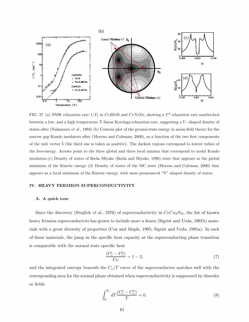
FIG. 27 (a) NMR relaxation rate 1/T1 in CeRhSb and CeNiSn, showing a T 3 relaxation rate sandwiched
between a low, and a high temperature T -linear Korringa relaxation rate, suggesting a V - shaped density of
states after (Nakamura et al., 1994) (b) Contour plot of the ground-state energy in mean-field theory for the
narrow gap Kondo insulators after (Moreno and Coleman, 2000), as a function of the two first components
of the unit vector b (the third one is taken as positive). The darkest regions correspond to lowest values of
the free-energy. Arrows point to the three global and three local minima that correspond to nodal Kondo
insulators.(c) Density of states of Ikeda Miyake (Ikeda and Miyake, 1996) state that appears as the global
minimum of the Kinetic energy (d) Density of states of the MC state (Moreno and Coleman, 2000) that
appears as a local minimum of the Kinetic energy, with more pronounced “V” shaped density of states.
IV. HEAVY FERMION SUPERCONDUCTIVITY
A. A quick tour
Since the discovery (Steglich et al., 1976) of superconductivity in CeCu2Si2, the list of known
heavy fermion superconductors has grown to include more a dozen (Sigrist and Ueda, 1991b) mate-
rials with a great diversity of properties (Cox and Maple, 1995; Sigrist and Ueda, 1991a). In each
of these materials, the jump in the specific heat capacity at the superconducting phase transition
is comparable with the normal state specific heat
(Csv − Cn
v)
CV∼ 1 − 2, (7)
and the integrated entropy beneath the Cv/T curve of the superconductor matches well with the
corresponding area for the normal phase obtained when superconductivity is suppressed by disorder
or fields∫ Tc
0dT
(Csv − Cnv )
T= 0. (8)
61
Since the normal state entropy is derived from the f-moments, it follows that these same degrees
of freedom are involved in the development of the superconducting state. With the exception of a
few anomalous cases, (UBe13, PuCoGa5 and CeCoIn5) heavy fermion superconductivity develops
out of the coherent, paramagnetic heavy Fermi liquid, so heavy fermion superconductivity can be
said to involve the pairing of heavy f-electrons.
Independent confirmation of the “heavy” nature of the pairing electrons comes from observed
size of the London penetration depth λL and superconducting coherence length ξ in these systems,
both of which reflect the enhanced effective mass, The large mass renormalization enhances the
penetration depth, whilst severely contracting the coherence length, making these extreme type-II
superconductors. The London penetration depth of heavy fermion superconductors agree well with
the value expected on the assumption that only spectral weight in the quasiparticle Drude peak
condenses to form a superconductor by
1
µoλ2L
=ne2
m∗ =
∫
ω∈D.P
dω
πσ(ω) <<
ne2
m(9)
London penetration depths in these compounds are a factor of 20−30 times longer (Broholm et al.,
1990) than in superconductors, reflecting the large enhancement in effective mass. By contrast,
the coherence lengths ξ ∼ vF /∆ ∼ hkF /(m∗∆) are severely contracted in a heavy fermion super-
conductor. The orbitally limited upper critical field is determined by the condition that an area
ξ2 contains a flux quantum ξ2Bc ∼ h2e . In UBe13, a superconductor with 0.9K transition temper-
ature, the upper critical field is about 11 Tesla, a value about 20 times larger than a conventional
superconductor of the same transition temperature.
Table B. shows a selected list of heavy fermion superconductors. “Canonical” heavy fermion
superconductors, such as CeCu2Si2 and UPt3, develop superconductivity out of a paramag-
netic Landau Fermi liquid. “Pre-ordered” superconductors, such as UPt2Al3 (Geibel et al., 1991;
Geibel. et al., 1991), CePt3Si and URu2Si2, develop another kind of order before going supercon-
ducting at a lower temperature. In the case of URu2Si2, the nature of the upper ordering transition
is still unidentified. but in the other examples, the upper transition involves the development of an-
tiferromagnetism. “Quantum critical” superconductors, including CeIn3 and CeCu2(Si1−xGex)2
develop superconductivity when pressure tuned close to a quantum critical point. CeIn3 devel-
ops superconductivity at the pressure-tuned antiferromagnetic quantum critical point at 2.5GPa
(25kbar). CeCu2(Si,Ge)2 has two islands, one associated with antiferromagnetism at low pressure,
and a second at still higher pressure, thought to be associated with critical valence fluctuations
(Yuan et al., 2006).
62

Table. B. Selected Heavy Fermion Superconductors.
TypeMaterial Tc Knight Shift Remarks Gap
Symmetry
Ref.
(Singlet)
“Canonical”
CeCu2Si2 0.7 Singlet First HFSC Line nodes [1]
UPt3 0.48K ?Double Transition to
T-violating state
Line and
point nodes[2]
Pre-ordered
UPd2Al3 2K SingletNeel AFM
TN = 14K
Line nodes
∆ ∼ cos 2χ[3]
URu2Si2 1.3K SingletHidden order at
T0 = 17.5KLine nodes [4]
CePt3Si 0.8KSinglet and
Triplet
Parity-violating xtal.
TN = 3.7KLine nodes [5]
Quantum
Critical
CeIn3
0.2K
(2.5GPa)Singlet
First quantum critical
HFSCLine nodes [6]
CeCu2(Si1−xGex)20.4K (P=0)
0.95K(5.4GPa)Singlet
Two islands of SC as
function of pressureLine nodes. [7]
Quadrupolar PrOs4Sb12 1.85K SingletQuadrupolar
fluctuationsPoint nodes [8]
“Strange”
CeCoIn5 2.3K SingletQuasi-2D
ρn ∼ T
Line nodes
dx2−y2[9]
UBe13 0.86K ? Incoherent metal at Tc. Line nodes [10]
PuCoGa5 18.5K SingletDirect transition Curie
metal → HFSCLine nodes [11]
[1] (Steglich et al., 1976), [2] (Stewart et al., 1984a), [3] (Geibel et al., 1991; Sato et al., 2001; Tou et al.,
1995), [4] (Kim et al., 2003; Palstra et al., 1985), [5] (Bauer et al., 2004), [6] (Mathur et al., 1998), [7]
(Yuan et al., 2006), [8] (Isawa et al., 2003), [9] (Petrovic et al., 2001), [10] (Andres et al., 1975), [11]
(Sarrao et al., 2002).
“Strange” superconductors, which include UBe13, the 115 material CeCoIn5 and PuCoGa5,
condense into the superconducting state out of an incoherent or strange metallic state. UBe13 has a
63

resistance of order 150µΩcm at its transition temperature. CeCoIn5 bears superficial resemblance
to a high temperature superconductor, with a linear temperature resistance in its normal state,
while its cousin, PuCoGa5 transitions directly from a Curie paramagnet of unquenched f-spins into
an anisotropically paired, singlet superconductor. These particular materials severely challenge
our theoretical understanding, for the heavy electron quasiparticles appear to form as part of the
condensation process, and we are forced to address how the f-spin degrees of freedom incorporate
into the superconducting parameter.
B. Phenomenology
The main body of theoretical work on heavy electron systems is driven by experiment, and
focuses directly on the phenomenology of the superconducting state. For these purposes, it is
generally sufficient to assume a Fermi liquid of pre-formed mobile heavy electrons, an electronic
analog of superfluid Helium-3, in which the quasiparticles interact through a phenomenological BCS
model. For most purposes, Landau Ginzburg theory is sufficient. I regret that in this short review,
I do tno have time to properly represent and discuss the great wealth of fascinating phenomenology
- the wealth of multiple phases, and the detailed models that have been developed to describe them.
I refer the interested reader to reviews on this subject. (Sigrist and Ueda, 1991a).
On theoretical grounds, the strong Coulomb interactions of the f-electrons that lead to mo-
ment formation in heavy fermion compounds are expected to heavily suppress the formation of
conventional s-wave pairs in these systems. A large body of evidence favors the idea that the gap
function and the anomalous Green function between paired heavy electrons Fαβ(x) = 〈c†α(x)c†β(0)〉is spatially anisotropic, forming either p-wave triplet, or d-wave singlet pairs.
In BCS theory, the superconducting quasiparticle excitations are determined by a one-particle
Hamiltonian of the form
H =∑
k,σ
ǫkf†kαfkα +
∑
k
[f †kα∆αβ(k)f †−kβ + f−kβ∆βα(k)fkα]
where
∆αβ(k) =
∆(k)(iσ2)αβ (singlet),
~d(k) · (iσ2~σ)αβ (triplet).
For singlet pairing, ∆(k) is an even parity function of k while for triplet pairing, ~d(k) is a an
odd-parity function of k with three components.
64
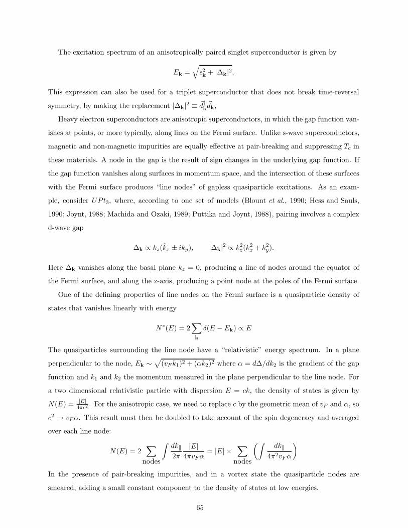
The excitation spectrum of an anisotropically paired singlet superconductor is given by
Ek =√
ǫ2k + |∆k|2,
This expression can also be used for a triplet superconductor that does not break time-reversal
symmetry, by making the replacement |∆k|2 ≡ ~d†k~dk,
Heavy electron superconductors are anisotropic superconductors, in which the gap function van-
ishes at points, or more typically, along lines on the Fermi surface. Unlike s-wave superconductors,
magnetic and non-magnetic impurities are equally effective at pair-breaking and suppressing Tc in
these materials. A node in the gap is the result of sign changes in the underlying gap function. If
the gap function vanishes along surfaces in momentum space, and the intersection of these surfaces
with the Fermi surface produces “line nodes” of gapless quasiparticle excitations. As an exam-
ple, consider UPt3, where, according to one set of models (Blount et al., 1990; Hess and Sauls,
1990; Joynt, 1988; Machida and Ozaki, 1989; Puttika and Joynt, 1988), pairing involves a complex
d-wave gap
∆k ∝ kz(kx ± iky), |∆k|2 ∝ k2z(k
2x + k2
y).
Here ∆k vanishes along the basal plane kz = 0, producing a line of nodes around the equator of
the Fermi surface, and along the z-axis, producing a point node at the poles of the Fermi surface.
One of the defining properties of line nodes on the Fermi surface is a quasiparticle density of
states that vanishes linearly with energy
N∗(E) = 2∑
k
δ(E − Ek) ∝ E
The quasiparticles surrounding the line node have a “relativistic” energy spectrum. In a plane
perpendicular to the node, Ek ∼√
(vF k1)2 + (αk2)2 where α = d∆/dk2 is the gradient of the gap
function and k1 and k2 the momentum measured in the plane perpendicular to the line node. For
a two dimensional relativistic particle with dispersion E = ck, the density of states is given by
N(E) = |E|4πc2
. For the anisotropic case, we need to replace c by the geometric mean of vF and α, so
c2 → vFα. This result must then be doubled to take account of the spin degeneracy and averaged
over each line node:
N(E) = 2∑
nodes
∫dk‖2π
|E|4πvFα
= |E| ×∑
nodes
(∫dk‖
4π2vFα
)
In the presence of pair-breaking impurities, and in a vortex state the quasiparticle nodes are
smeared, adding a small constant component to the density of states at low energies.
65

This linear density of states is manifested in a variety of power laws in the temperature depen-
dence of experimental properties, most notably
• Quadratic temperature dependence of specific heat CV ∝ T 2, since the specific heat coeffi-
cient is proportional to the thermal average of the density of states
CVT
∝∝T
︷ ︸︸ ︷
N(E) ∼ T
where N(E) denotes the thermal average of N(E).
• A ubiquitous T 3 temperature dependence in the nuclear magnetic and quadrapole relaxation
(NMR/NQR) relaxation rates 1/T1. The nuclear relaxation rate is proportional to the
thermal average of the squared density of states, so for a superconductor with line nodes,
1
T1∝ T
∝T 2
︷ ︸︸ ︷
N(E)2 ∼ T 3
Fig. 28 shows the T 3 NMR relaxation rate of the Aluminum nucleus in UPd2Al3.
Although power-laws can distinguish line and point nodes, they do not provide any detailed
information about the triplet or singlet character of the order parameter, or the location of the
nodes. The observation of upper critical fields that are “Pauli limited” (set by the spin coupling,
rather than the diamagnetism), and the observation of a Knight shift in most heavy fermion
superconductors, indicates that they are anisotropically singlet paired. Three notable exceptions
to this rule are UPt3, UBe13 and UNi2Al3, which do not display either a Knight shift or a Pauli-
limited upper critical field, are the best candidates for odd-parity triplet pairing. In the special
case of CePt3Sn, the crystal structure lacks a center of symmetry and the resulting parity violation
is must give a mixture of triplet and singlet pairs.
Until comparatively recently, very little was known about the positions of the line nodes in heavy
electron superconductors. In one exception, experiments carried out almost twenty years ago on
UPt3 observed marked anisotropies in the ultrasound attenuation length and the penetration depth,
(Bishop et al., 1984; Broholm et al., 1990) that appear to support a line of nodes in the basal plane.
The ultrasonic attenuation αs(T )/αn in single crystals of UPt3 has a T linear dependence when
the polarization lies in the basal plane of the gap nodes but a T 3 dependence when the polarization
is along the c-axis.
An interesting advance in the experimental analysis of nodal gap structure has recently occurred,
thanks to new insights into the behavior of the nodal excitation spectrum in the flux phase of heavy
66

FIG. 28 Temperature dependence of the 27Al NQR relaxation rate 1/T1 for UPd2Al3 after (Tou et al.,
1995) showing T 3 dependence associated with lines of nodes. Inset showing nodal structure ∆ ∝ cos(2θ)
proposed from analysis of anisotropy of thermal conductivity in (Won et al., 2004).
fermion superconductors. In the nineties, Volovik (Volovik, 1993) observed that the energy of heavy
electron quasiparticles in a flux lattice is “Doppler shifted” by the superflow around the vortices,
giving rise to a finite density of quasiparticle states around the gap nodes. The Doppler shift in
the quasiparticle energy resulting from superflow is given by
Ek → Ek + ~p · ~vs = Ek + ~vF · h2~∇φ
where ~vs is the superfluid velocity and φ the superfluid phase. This has the effect of shifting
quasiparticle states by an energy of order ∆E ∼ h vF
2R , where R is the average distance between
vortices in the flux lattice. Writing πHR2 ∼ Φ0, and πHc2ξ2 ∼ Φ0 where Φ0 = h
2e is the flux
quantum, Hc2 is the upper critical field and ξ is the coherence length. it follows that 1R ∼ 1
ξ
√HHc2
.
Putting ξ ∼ vF /∆, where ∆ is the typical size of the gap, the typical shift in the energy of nodal
quasiparticles is of order EH ∼ ∆√
HHc2
. Now since the density of states is of orderN(E) = |E|∆ N(0),
where N(0) is the density of states in the normal phase. it follows that the smearing of the nodal
67

quasiparticle energies will produce a density of states of order
N∗(H) ∼ N(0)
√
H
Hc2
This effect, the “Volovik effect”, produces a linear component to the specific heat CV /T ∝√
HHc2
.
This enhancement of the density of states is largest when the group velocity ~VF at the node is
perpendicular to the applied field ~H, and when the field is parallel to ~vF at a particular node, the
node is unaffected by the vortex lattice (Fig. 29). This gives rise to an angular dependence in the
specific heat coefficient and thermodynamics that can be used to measure the gap anisotropy. In
practice, the situation is complicated at higher fields where the Andreev scattering of quasiparticles
by vortices becomes important. The case of CeCoIn5 is of particular current interest. Analyses
of the field-anisotropy of the thermal conductivity in this material was interpreted early on in
terms of a gap structure with dx2−y2 , while the anisotropy in the specific heat appears to suggest a
dxy symmetry. Recent theoretical work by Vorontsev and Vekhter (Vorontsov and Vekhter, 2006)
suggests that the discrepancy between the two interpretations can be resolved by taking into
account the effects of the vortex quasiparticle scattering that were ignored in the specific heat
interpretation. They predict that at lower fields, where vortex scattering effects are weaker, the
sign of the anisotropic term in the specific heat will reverse, accounting for the discrepancy
It is clear that, despite the teething problems in the interpretation of field-anisotropies in trans-
port and thermodynamics, this is an important emerging tool for the analysis of gap anisotropy,
and to date, it has been used to give tentative assignments to the gap anisotropy of UPd2Al3,
CeCoIn5 and PrOs4Sb12.
C. Microscopic models
1. Antiferromagnetic fluctuations as a pairing force.
The classic theoretical models for heavy fermion superconductivity treat the heavy electron flu-
ids as a Fermi liquid with antiferromagnetic interactions amongst their quasiparticles (Monod et al.,
1986; Monthoux and Lonzarich, 1999; Scalapino et al., 1986). UPt3 provided the experimental in-
spiration for early theories of heavy fermion superconductivity, for its superconducting state forms
from within a well-developed Fermi liquid. Neutron scattering on this material shows signs of an-
tiferromagnetic spin fluctuations (Aeppli et al., 1987), making it natural to presuppose that these
might be the driving force for heavy electron pairing.
68
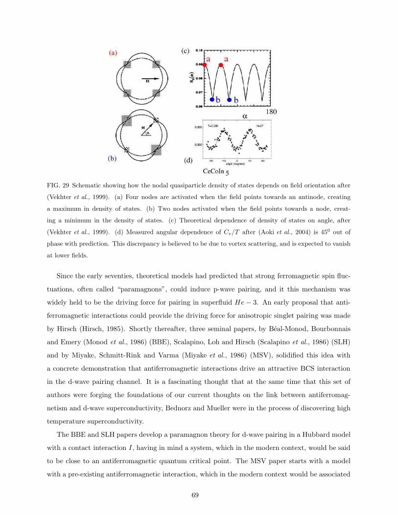
FIG. 29 Schematic showing how the nodal quasiparticle density of states depends on field orientation after
(Vekhter et al., 1999). (a) Four nodes are activated when the field points towards an antinode, creating
a maximum in density of states. (b) Two nodes activated when the field points towards a node, creat-
ing a minimum in the density of states. (c) Theoretical dependence of density of states on angle, after
(Vekhter et al., 1999). (d) Measured angular dependence of Cv/T after (Aoki et al., 2004) is 450 out of
phase with prediction. This discrepancy is believed to be due to vortex scattering, and is expected to vanish
at lower fields.
Since the early seventies, theoretical models had predicted that strong ferromagnetic spin fluc-
tuations, often called “paramagnons”, could induce p-wave pairing, and it this mechanism was
widely held to be the driving force for pairing in superfluid He− 3. An early proposal that anti-
ferromagnetic interactions could provide the driving force for anisotropic singlet pairing was made
by Hirsch (Hirsch, 1985). Shortly thereafter, three seminal papers, by Beal-Monod, Bourbonnais
and Emery (Monod et al., 1986) (BBE), Scalapino, Loh and Hirsch (Scalapino et al., 1986) (SLH)
and by Miyake, Schmitt-Rink and Varma (Miyake et al., 1986) (MSV), solidified this idea with
a concrete demonstration that antiferromagnetic interactions drive an attractive BCS interaction
in the d-wave pairing channel. It is a fascinating thought that at the same time that this set of
authors were forging the foundations of our current thoughts on the link between antiferromag-
netism and d-wave superconductivity, Bednorz and Mueller were in the process of discovering high
temperature superconductivity.
The BBE and SLH papers develop a paramagnon theory for d-wave pairing in a Hubbard model
with a contact interaction I, having in mind a system, which in the modern context, would be said
to be close to an antiferromagnetic quantum critical point. The MSV paper starts with a model
with a pre-existing antiferromagnetic interaction, which in the modern context would be associated
69

with the “t-J” model. It is this approach that I sketch here. The MSV model is written
H =∑
ǫka†kσakσ +Hint (117)
where
Hint =1
2
∑
k,k′
∑
q
J(k − k′)~σαβ · ~σγδ ×(
a†k+q/2αa
†−k+q/2γ
)(
a−k′+q/2δak′+q/2β
)
(118)
describes the antiferromagnetic interactions. There are a number of interesting points to be made
here:
• The authors have in mind a strong coupled model, such as the Hubbard model at large U
where the interaction can not be simply derived from paramagnon theory. In a weak-coupled
Hubbard model a contact interaction I and bare susceptibility χ0(q), the induced magnetic
interaction can be calculated in an RPA approximation (Miyake et al., 1986) as
J(q) = − I
2[1 + Iχ0(q)].
MSV make the point that the detailed mechanism that links the low-energy antiferromagnetic
interactions to the microscopic interactions is poorly described by a weak-coupling theory,
and quite likely to involve other processes, such as the RKKY interaction, and the Kondo
effect that lie outside this treatment.
• Unlike phonons, magnetic interactions in heavy fermion systems can not generally be re-
garded as retarded interactions, for they extend up to an energy scale ω0 that is comparable
with the heavy electron band-width T ∗. In a classic BCS treatment, the electron energy
are restricted to lie within a Debye energy of the Fermi energy. But here, ω0 ∼ T ∗, so all
momenta are involved in magnetic interactions, and the interaction can transformed to real
space as
H =∑
ǫka†kσakσ +
1
2
∑
i,j
J(Ri − Rj)~σi · ~σj (119)
where J(R) =∑
q eiq·RJ(q) is the Fourier transform of the interaction and ~σi = a†iα~σαβaiβ
is the spin density at site i. Written in real space, the MSV model is seen to be an early
predecessor of the t − J model used extensively in the context of high temperature super-
conductivity.
70
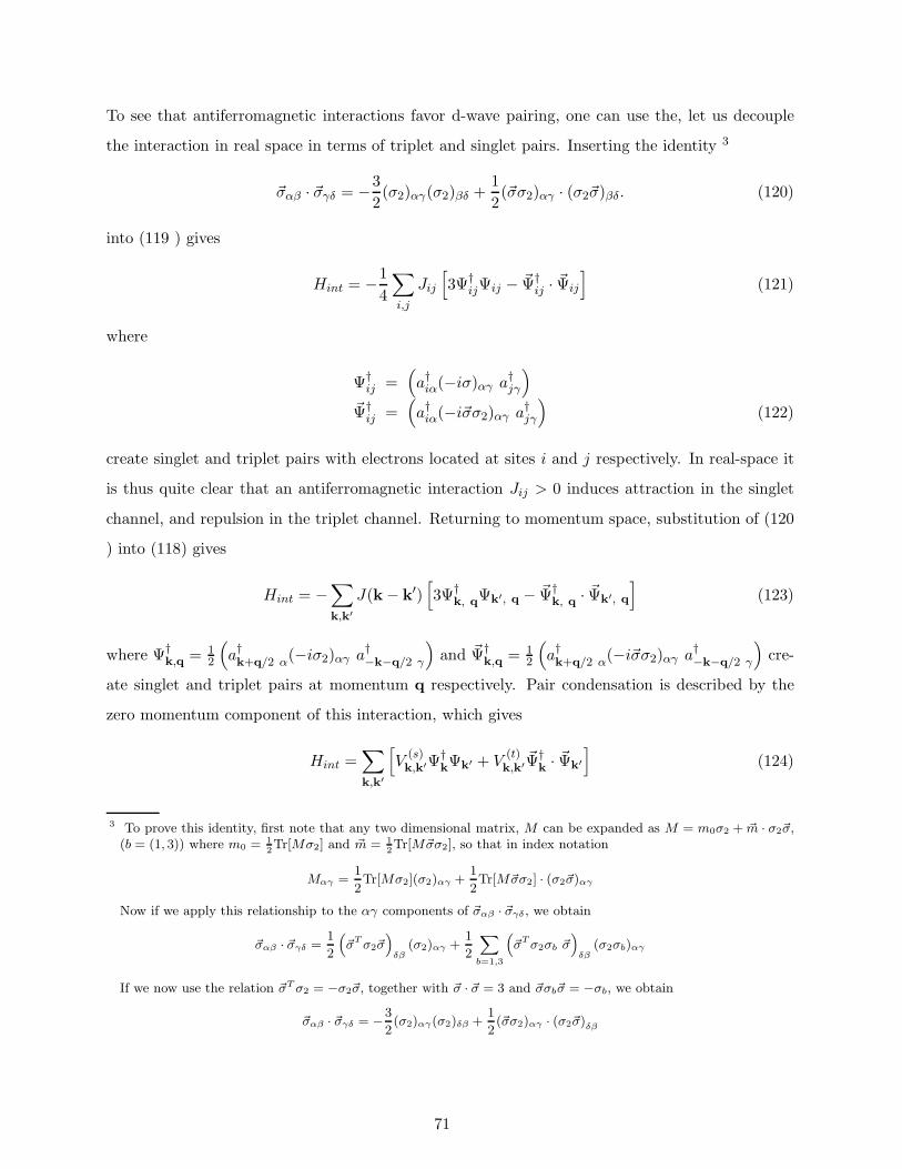
To see that antiferromagnetic interactions favor d-wave pairing, one can use the, let us decouple
the interaction in real space in terms of triplet and singlet pairs. Inserting the identity 3
~σαβ · ~σγδ = −3
2(σ2)αγ(σ2)βδ +
1
2(~σσ2)αγ · (σ2~σ)βδ. (120)
into (119 ) gives
Hint = −1
4
∑
i,j
Jij
[
3Ψ†ijΨij − ~Ψ†
ij · ~Ψij
]
(121)
where
Ψ†ij =
(
a†iα(−iσ)αγ a†jγ
)
~Ψ†ij =
(
a†iα(−i~σσ2)αγ a†jγ
)
(122)
create singlet and triplet pairs with electrons located at sites i and j respectively. In real-space it
is thus quite clear that an antiferromagnetic interaction Jij > 0 induces attraction in the singlet
channel, and repulsion in the triplet channel. Returning to momentum space, substitution of (120
) into (118) gives
Hint = −∑
k,k′
J(k − k′)[
3Ψ†k, qΨk′, q − ~Ψ†
k, q · ~Ψk′, q
]
(123)
where Ψ†k,q = 1
2
(
a†k+q/2 α(−iσ2)αγ a
†−k−q/2 γ
)
and ~Ψ†k,q = 1
2
(
a†k+q/2 α(−i~σσ2)αγ a
†−k−q/2 γ
)
cre-
ate singlet and triplet pairs at momentum q respectively. Pair condensation is described by the
zero momentum component of this interaction, which gives
Hint =∑
k,k′
[
V(s)k,k′Ψ
†kΨk′ + V
(t)k,k′
~Ψ†k · ~Ψk′
]
(124)
3 To prove this identity, first note that any two dimensional matrix, M can be expanded as M = m0σ2 + ~m · σ2~σ,(b = (1, 3)) where m0 = 1
2Tr[Mσ2] and ~m = 1
2Tr[M~σσ2], so that in index notation
Mαγ =1
2Tr[Mσ2](σ2)αγ +
1
2Tr[M~σσ2] · (σ2~σ)αγ
Now if we apply this relationship to the αγ components of ~σαβ · ~σγδ , we obtain
~σαβ · ~σγδ =1
2
“
~σT σ2~σ”
δβ(σ2)αγ +
1
2
X
b=1,3
“
~σT σ2σb ~σ”
δβ(σ2σb)αγ
If we now use the relation ~σT σ2 = −σ2~σ, together with ~σ · ~σ = 3 and ~σσb~σ = −σb, we obtain
~σαβ · ~σγδ = −3
2(σ2)αγ(σ2)δβ +
1
2(~σσ2)αγ · (σ2~σ)δβ
71

where Ψ†k = 1
2
(
a†kα(−iσ2)αβ a†−kβ
)
and ~Ψ†k,q = 1
2
(
a†kα(−i~σσ2)αβ a†−kβ
)
create Cooper pairs and
Vs)k,k′ = −3[J(k − k′) + J(k + k′)]/2
V(t)k,k′ = [J(k − k′) − J(k + k′)]/2 (125)
are the BCS pairing potentials in the singlet, and triplet channel respectively. (Notice how the
even/odd parity symmetry of the triplet pairs pulls out the corresponding symmetrization of J(k−k′))
For a given choice of J(q), it now becomes possible to decouple the interaction in singlet and
triplet channels. For example, on a cubic lattice of side length, if the magnetic interaction has the
form
J(q) = 2J(cos(qxa) + cos(qya) + cos(qza))
which generates soft antiferromagnetic fluctuations at the staggered Q vector Q = (π/a, π/a, π/a),
then the pairing interaction can be decoupled into singlet and triplet components,
V sk,k′ = −3J
2
[s(k)s(k′) + dx2−y2(k)dx2−y2(k
′) + d2z2−r2(k)d2z2−r2(k′)]
V tk,k′ =
J
2
∑
i=x,y,z
pi(k)pi(k′) (126)
where
s(k) =√
23(cos(kxa) + cos(kya) + cos(kza)) (extended s-wave)
dx2−y2(k) = (cos(kxa) − cos(kya),
d2z2−r2(k) = 1√3(cos(kxa) + cos(kya) − 2 cos(kza))
(d-wave)
(127)
are the gap functions for singlet pairing and
pi(q) =√
2 sin(qia), (i = x, y, z), (p-wave) (128)
describe three triplet gap functions. For J > 0, this particular BCS model will then give rise to
extended s and d-wave superconductivity with approximately the same transition temperatures,
given by the gap equation
∑
k
tanh
(ǫk2Tc
)1
ǫk
s(k)2
dx2−y2(k)2
=
2
3J
72

2. Towards a unified theory of HFSC
Although the spin fluctuation approach described provides a good starting point for the phe-
nomenology of heavy fermion superconductivity, it leaves open a wide range of questions that
suggest this problem is only partially solved:
• How can we reconcile heavy fermion superconductivity with the local moment origins of the
heavy electron quasiparticles?
• How can the the incompressibility of the heavy electron fluid be incorporated into the theory?
In particular, extended s-wave solutions are expected to produce a large singlet f-pairing
amplitude, giving rise to a large Coulomb energy. Interactions are expected to significantly
depress, if not totally eliminate such extended s-wave solutions.
• Is there a controlled limit where a model of heavy electron superconductivity can be solved?
• What about the “strange” heavy fermion superconductors UBe13, CeCoIn5 and PuCoGa5,
where Tc is comparable with the Kondo temperature? In this case, the superconducting
order parameter must involve the f-spin as a kind of “composite” order parameter. What is
the nature of this order parameter, and what physics drives Tc so high that the Fermi liquid
forms at much the same time as the superconductivity develops?
One idea that may help to understand the heavy fermion pairing mechanism is Anderson’s
resonating valence bond (RVB) theory (Anderson, 1987) of high temperature superconductivity.
Anderson proposed (Anderson, 1987; Baskaran et al., 1987; Kotliar, 1988) that the parent state of
the high temperature superconductors is a two-dimensional spin liquid of resonating valence bonds
between spins, which becomes superconducting upon doping with holes. In the early nineties, Cole-
man and Andrei (Coleman and Andrei, 1989) adapted this theory to a Kondo lattice. Although an
RVB spin-liquid is unstable with respect to antiferromagnetic order in three dimensions, in situa-
tions close to a magnetic instability, where the energy of the antiferromagnetic state is comparable
with the Kondo temperature, EAFM ∼ TK , conduction electrons will partially spin-compensate
the spin liquid, stabilizing it against magnetism (Fig. 30 (a)). In the Kondo-stabilized spin liquid,
the Kondo effect induces some resonating valence bonds in the f-spin liquid to escape into the
conduction fluid where they pair charged electrons to form a heavy electron superconductor.
A key observation of RVB theory is that when charge fluctuations are removed to form a spin
fluid, there is no distinction between particle and hole (Affleck et al., 88). The mathematical
73
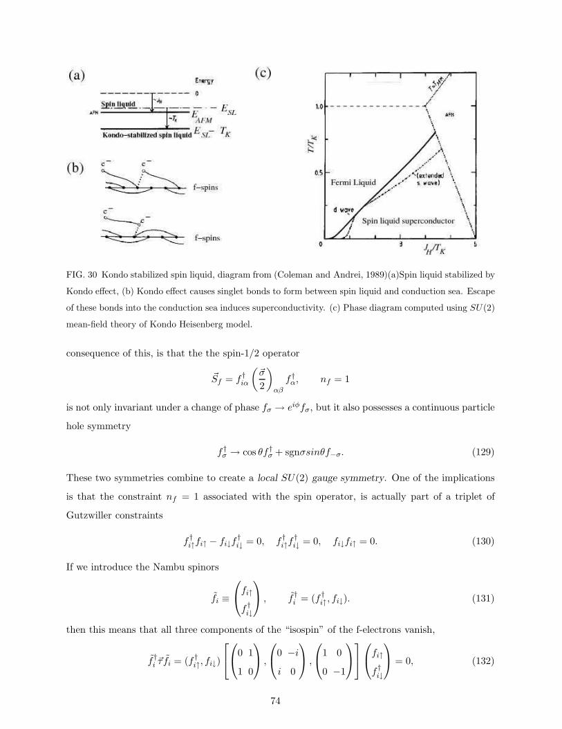
FIG. 30 Kondo stabilized spin liquid, diagram from (Coleman and Andrei, 1989)(a)Spin liquid stabilized by
Kondo effect, (b) Kondo effect causes singlet bonds to form between spin liquid and conduction sea. Escape
of these bonds into the conduction sea induces superconductivity. (c) Phase diagram computed using SU(2)
mean-field theory of Kondo Heisenberg model.
consequence of this, is that the the spin-1/2 operator
~Sf = f †iα
(~σ
2
)
αβ
f †α, nf = 1
is not only invariant under a change of phase fσ → eiφfσ, but it also possesses a continuous particle
hole symmetry
f †σ → cos θf †σ + sgnσsinθf−σ. (129)
These two symmetries combine to create a local SU(2) gauge symmetry. One of the implications
is that the constraint nf = 1 associated with the spin operator, is actually part of a triplet of
Gutzwiller constraints
f †i↑fi↑ − fi↓f†i↓ = 0, f †i↑f
†i↓ = 0, fi↓fi↑ = 0. (130)
If we introduce the Nambu spinors
fi ≡
fi↑
f †i↓
, f †i = (f †i↑, fi↓). (131)
then this means that all three components of the “isospin” of the f-electrons vanish,
f †i ~τ fi = (f †i↑, fi↓)
0 1
1 0
,
0 −ii 0
,
1 0
0 −1
fi↑
f †i↓
= 0, (132)
74

where ~τ is a triplet of Pauli spin operators that act on the f- Nambu spinors. In other words, in
the incompressible f-fluid, there can be no s− wave singlet pairing.
This symmetry is preserved in spin-1/2 Kondo models. When applied to the Heisenberg Kondo
model
H =∑
~kσ
ǫ~kc†~kσc~kσ + JH
∑
(i,j)
Si · Sj + JK∑
j
c†jσ~σσσ′cjσ′ · Sj (133)
where Si = f †iα(~σ2
)
αβfiβ represents an f-spin at site i, it leads to an SU (2) gauge theory for the
Kondo lattice with Hamiltonian
H =∑
~kǫ~k c
†~kτ3c~k +
∑~λj f†j~τ fj +
∑
(i,j)[f†i Uij fj +H.c] + 1
JHTr[U †
ijUij ]
+∑
i[f†i Vici +H.c] + 1
JKTr[V †
i Vi]. (134)
where λj is the Lagrange multiplier that imposes the Gutzwiller constraint ~τ = 0 at each site,
ck =
(ck↑
c†−k↓
)
and cj =
(cj↑
c†j↓
)
are Nambu conduction electron spinors in the momentum, and
position basis, respectively, while
Uij =
hij ∆ij
∆ij −hij
, Vi =
Vi αi
αi −Vi
are matrix order parameters associated with the Heisenberg and Kondo decoupling, respectively.
This model has the local gauge invariance fj → gj fj, Vj → gjVj Uij → giUijg†j where gj is an SU(2)
matrix. In this kind of model, one can “gauge fix” the model so that the Kondo effect occurs in
the particle-hole channel (αi = 0). When one does so however, the spin-liquid instability takes
place preferentially in an anisotropically paired Cooper channel. Moreover, the constraint on the
f-electrons not only suppresses singlet s-wave pairing, it also suppresses extended s-wave pairing
(Fig. 30 ).
One of the initial difficulties with both the RVB and the Kondo stabilized-spin liquid approaches
is that in its original formulation, it could not be integrated into a large N approach. Recent
work indicates that both the fermionic RVB and the Kondo stabilized spin liquid picture can be
formulated as a controlled SU(2) gauge theory by carrying out a large N expansion using the group
SP (N) (Read and Sachdev, 1991), originally introduced by Read and Sachdev for problems in
frustrated magnetism, in place of the group SU(N). The local particle-hole symmetry associated
with the spin operators in SU(2) is intimately related to the symplectic property of Pauli spin
operators
σ2~σTσ2 = −~σ (135)
75

FIG. 31 Temperature dependence of the magnetic susceptibility of PuCoGa5 after (Sarrao et al., 2002). The
susceptibility shows a direct transition from Curie Weiss paramagnet into heavy fermion superconductor,
without any intermediate spin quenching.
where ~σT is the transpose of the spin operator. This relation, which represents the sign reversal
of spin operators under time-reversal, is only satisfied by a subset of the SU(N) spins for N > 2.
This subset defines the generators of the symplectic subgroup of SU(N), called SP (N).
Concluding this section, I want to briefly mention the challenge posed by the highest Tc su-
perconductor, PuCoGa5 (Curro et al., 2005; Sarrao et al., 2002). This material, discovered some
four years ago at Los Alamos, undergoes a direct transition from a Curie paramagnet into a heavy
electron superconductor at around Tc = 19K (Fig.31). The Curie paramagnetism is also seen
in the Knight-shift, which scales with the bulk susceptibility (Curro et al., 2005). The remark-
able feature of this material, is that the specific heat anomaly has the large size (110mJ/mol/K2
(Sarrao et al., 2002)) characteristic of heavy fermion superconductivity, yet there there are no signs
of saturation in the susceptibility as a precursor to superconductivity, suggesting that the heavy
quasiparticles do not develop from local moments until the transition. This aspect of the physics
can not be explained by spin-fluctuation theory(Bang et al., 2004), and suggests that the Kondo
effect takes place simultaneously with the pairing mechanism. One interesting possibility here, is
that the development of coherence between the Kondo effect in two different channels created by
the different symmetries of the valence fluctuations into the f6 and f4 states might be the driver
of this intriguing new superconductor (Coleman et al., 1999; Jarrell et al., 1997).
76

V. QUANTUM CRITICALITY
A. Singularity in the Phase diagram
Many heavy electron systems can be tuned, with pressure, chemical doping or applied mag-
netic field, to a point where their antiferromagnetic ordering temperature is driven continuously
to zero to produce a “quantum critical point” (Coleman et al., 2001; von Lohneysen et al., 2007;
Miranda and Dobrosavljevic, 2005; Stewart, 2001, 2006; Varma et al., 2002). The remarkable
transformation in metallic properties, often referred to as “non-Fermi liquid behavior”, that is
induced over a wide range of temperatures above the quantum critical point (QCP), together with
the marked tendency to develop superconductivity in the vicinity of such “quantum critical points”
has given rise to a resurgence of interest in heavy fermion materials.
The experimental realization of quantum criticality returns us to central questions left unan-
swered since the first discovery of heavy fermion compounds. In particular:
• What is the fate of the Landau quasiparticle when interactions become so large that the
ground state is no longer adiabatically connected to a non-interacting system?
• What is the mechanism by which the antiferromagnet transforms into the heavy electron
state? Is there a break-down of the Kondo effect, revealing local moments at the quantum
phase transition, or is the transition better regarded as a spin density wave transition?
Fig. 32. illustrates quantum criticality in Y bRh2Si2(Custers et al., 2003), a material with a
90mK magnetic transition that can be tuned continuously to zero by a modest magnetic field.
In wedge-shaped regions either side of the transition, the resistivity displays the T 2 dependence
ρ(T ) = ρ0 +AT 2 (colorcoded blue) that is the hallmark of Fermi liquid behavior. Yet in a tornado
shaped region that stretches far above the QCP to about 20K, the resistivity follows a linear
dependence over more than three decades. The QCP thus represents a kind of “singularity” in the
material phase diagram.
Experimentally, quantum critical heavy electron materials fall between two extreme limits that
I shall call “hard” and “soft” quantum criticality. “Soft” quantum critical systems are moderately
well described in terms quasiparticles interacting with the soft quantum spin fluctuations created
by a spin-density wave instability. Theory predicts (Moriya and Kawabata, 1973) that in a three
dimensional metal, the quantum spin density wave fluctuations give rise to a weak√T singularity
77

FIG. 32 (a) Color coded plot of the logarithmic derivative of resistivity d ln ρ/d lnT after (Custers et al.,
2003)(b) Resistivity of Y bRh2Si2 in zero magnetic field, after (Trovarelli et al., 2000). Inset shows logarith-
mic derivative of resistivity
in the low temperature behavior of the specific heat coefficient
CVT
= γ0 − γ1
√T
Examples of such behavior include CeNi2Ge2 (Grosche et al., 2000; Kuchler et al., 2003) chemi-
cally doped Ce2−xLaxRu2Si2 and “A”-type antiferromagnetic phases of CeCu2Si2 at a pressure-
tuned QCP.
At the other extreme, in “hard” quantum critical heavy materials, many aspects of the
physics appear consistent with a break-down of the Kondo effect associated with a re-
localization of the f-electrons into ordered, ordered local moments beyond the QCP. Some of
the most heavily studied examples of this behavior occur in the chemically tuned QCP in
CeCu6−xAux (von Lohneysen, 1996; von Lohneysen et al., 1994; Schroeder et al., 1998, 2000). and
Y bRh2Si2−xGex (Custers et al., 2003; Gegenwart et al., 2005) and the field-tuned tuned QCP
s of Y bRh2Si2 (Trovarelli et al., 2000) and Y bAgGe(Bud’ko et al., 2004, 2005; Fak et al., 2005;
Niklowitz et al., 2006) Hallmarks of hard quantum criticality include a logarithimically diverging
specific heat coefficient at the QCP,
CvT
∼ 1
T0ln
(T0
T
)
(136)
and a quasi-linear resistivity
ρ(T ) ∼ T 1+η (137)
where η is in the range 0 − 0.2. The most impressive results to date have been observed at field-
tuned quantum critical points in Y bRh2Si2 and CeCoIn5, where linear resistivity has been seen
78

to extend over more than two decades of temperature at the field-tuned quantum critical point
(Paglione et al., 2003, 2006; Ronning et al., 2006; Steglich et al., 1976). Over the range where
linear , where the ratio between the change in the size of the resistivity ∆ρ to the zero temperature
(impurity driven) resistivity ρ0
∆ρ/ρ0 >> 1.
CeCoIn5 is particularly interesting, for in this case, this resistance ratio exceeds 102 for current
flow along the c-axis (Tanatar et al., 2006). This observation excludes any explanation of that
attributes the unusual resistivity to an interplay between spin-fluctuation scattering and impurity
scattering (Rosch, 1999). Mysteriously, CeCoIn5 also exhibits a T 3/2 resistivity for resistivity
for current flow in the basal plane below about 2K (Tanatar et al., 2006). Nakasuji, Fisk and
Pines(Nakasuji et al., 2004) have proposed that this kind of behavior may derive from a two fluid
character to the underlying conduction fluid.
In quantum critical Y bRh2Si2−xGex, the specific heat coefficient develops a 1/T 1/3 divergence
at the very lowest temperature. In the approach to a quantum critical point, Fermi liquid behavior
is confined to an ever-narrowing range of temperature. Moreover, both the linear coefficient of the
specific heat and the the quadratic coefficient A of the resistivity appear to diverge (Estrela et al.,
2002; Trovarelli et al., 2000). Taken together, these results suggests that the Fermi temperature
renormalizes to zero and the quasiparticle effective masses diverge
T ∗F → 0,
m∗
m→ ∞ (138)
at the QCP of these three dimensional materials. A central property of the Landau quasiparti-
cle, is the existence of a finite overlap “Z”, or “wavefunction renormalization” between a single
quasiparticle state, denoted by |qp−〉 and a bare electron state denoted by |e−〉 = c†kσ|0〉,
Z = |〈e−|qp−〉|2 ∼ m
m∗ (139)
If the quasiparticle mass diverges, the overlap between the quasiparticle and the electron state from
which it is derived is driven to zero, signaling a complete break-down in the quasiparticle concept
at a “hard” quantum critical point (Varma et al., 2002).
Table. C. Selected Heavy Fermion compounds with quantum critical points.
79

Compound xc/HcCv
T ρ ∼ T a Γ(T ) = αCP
Other Ref.
“hard”
“soft”
CeCu6−xAux xc = 0.1 1T0
ln(
To
T
)T + c -
χ′′Q0
(ω, T ) =
1T 0.7F
[ωT
] [1]
Y bRh2Si2 Bc‖ = 0.66T T -Jump in Hall
constant.[2]
Y bRh2Si2−xGex xc = 0.11
T 1/3↔
1T0
ln(
To
T
) T T−0.7 [3]
Y bAgGeBc‖ = 9T
Bc⊥ = 5T
1T0
ln(
To
T
)T -
NFL over
range of fields[4]
CeCoIn5 Bc = 5T 1T0
ln(
T0
T
)T / T 1.5 -
ρc ∝ T ,
ρab ∝ T 1.5[5]
CeNi2Ge2 Pc = 0 γ0 − γ1
√T T 1.2−1.5 T−1 [6]
[1] (von Lohneysen, 1996; von Lohneysen et al., 1994; Schroeder et al., 1998, 2000), [2] (Paschen et al., 2004;
Trovarelli et al., 2000), [3] (Custers et al., 2003; Gegenwart et al., 2005), [4] (Bud’ko et al., 2004, 2005;
Fak et al., 2005; Niklowitz et al., 2006) [5] (Paglione et al., 2003, 2006; Ronning et al., 2006; Tanatar et al.,
2006), [6] (Grosche et al., 2000; Kuchler et al., 2003).
Table C. shows a tabulation of selected quantum critical materials. One interesting variable
that exhibits singular behavior at both hard and soft quantum critical points, is the Gruneisen
ratio. This quantity, defined as the ratio
Γ =α
C= − 1
V
∂ lnT
∂P
∣∣∣∣S
∝ 1
T ǫ
of the thermal expansion coefficient α = 1VdVdT to the specific heat C, diverges at a QCP. The
Gruneisen ratio is a sensitive measure of the rapid acquisition of entropy on warming away from
QCP. Theory predicts that ǫ = 1 at a 3D SDW QCP , as seen in CeNi2Ge2. In the “hard”
quantum critical material Y bRh2Si2−xGex, ǫ = 0.7 indicates a serious departure from a 3D spin
density wave instability (Kuchler et al., 2003).
B. Quantum, versus classical criticaltiy.
Figure 33. illustrates some key distinctions between classical and quantum criticality (Sachdev,
2007). Passage through a classical second-order phase transition is achieved by tuning the temper-
ature. Near the transition, the imminent arrival of order is signaled by the growth of droplets of
80

nascent order whose typical size ξ diverges at the critical point. Inside each droplet, fluctuations
of the order parameter exhibit a universal powerlaw dependence on distance
〈ψ(x)ψ(0)〉 ∼ 1
xd−2+η, (x << ξ). (140)
Critical matter “forgets” about its microscopic origins, for its thermodynamics, scaling laws and
correlation exponents associated with critical matter are so robust and universal that they recur
in such diverse contexts as the Curie point of iron or the critical point of water. At a conventional
critical point order parameter fluctuations are “classical”, for the characteristic energy of the critical
modes hω(q0), evaluated at a wavevector q0 ∼ ξ−1, innevitably drops below the thermal energy
hω(q0) << kBTc as ξ → ∞.
In the seventies various authors, notably Young (Young, 1975) and Hertz (Hertz, 1976) recog-
nized that when if the transition temperature of a continuous phase transition can be depressed
to zero, the critical modes become quantum mechanical in nature. The partition function for a
quantum phase transition is described by a Feynman integral over order parameter configurations
ψ(x, τ) in both space and imaginary time (Hertz, 1976; Sachdev, 2007)
Zquantum =∑
space-time configs
e−S[ψ], (141)
where the action
S[ψ] =
∫ hkBT
0dτ
∫ ∞
−∞ddxL[ψ(x, τ)], (142)
contains an integral of the Lagrangian L over an infinite range in space, but a finite time interval
lτ ≡h
kBT.
Near a QCP, bubbles of quantum critical matter form within a metal, with finite size ξx and
duration ξτ . (Fig. 33). These two quantities diverge as the quantum critical point is approached,
but the rates of divergence are related by a dynamical critical exponent (Hertz, 1976),
ξτ ∼ (ξx)z
One of the consequences of this scaling behavior, is that time counts as z spatial dimensions,
[τ ] = [Lz] in general.
At a classical critical point, temperature is a tuning parameter that takes one through the
transition. The role of temperature is fundamentally different at a quantum critical point: for it
sets the scale lτ ∼ 1/T in the time direction, introducing a finite size correction to the quantum
81

FIG. 33 Contrasting classical and quantum criticality in heavy electron systems. At a QCP an external
parameter P , such as pressure or magnetic field replaces temperature as the “tuning parameter”. Temper-
ature assumes the new role of a finite size cutoff lτ ∝ 1/T on the temporal extent of quantum fluctuations.
(A) Quantum critical regime, where lτ < ξtau probes the interior of the quantum critical matter (B) Fermi
liquid regime, where lτ > ξτ , where like soda, bubbles of quantum critical matter fleetingly form within a
Fermi liquid that is paramagnetic (B1), or antiferromagnetically ordered (B2).
critical point. When the temperature is raised, lτ reduces and the quantum fluctuations are probed
on shorter and shorter time-scales. There are then two regimes to the phase diagram,
(A) Quantum critical: lτ << ξτ (143)
where the physics probes the “interior” of the quantum critical bubbles, and
(B) Fermi liquid/AFM lτ >> ξτ (144)
where the physics probes the quantum fluid “outside” the quantum critical bubbles. The quan-
tum fluid that forms in this region is a sort of “quantum soda”, containing short-lived bubbles
of quantum critical matter surrounded by a paramagnetic (B1) or antiferromagnetically ordered
(B2) Landau Fermi liquid. Unlike a classical phase transition, in which the critical fluctuations
are confined to a narrow region either side of the transition, in a quantum critical region (A),
fluctuations persist up to temperatures where lτ becomes comparable the with the microscopic
short time cut-off in the problem (Kopp and Chakravarty, 2005) (which for heavy electron systems
is most likely, the single-ion Kondo temperature lτ ∼ h/TK).
82
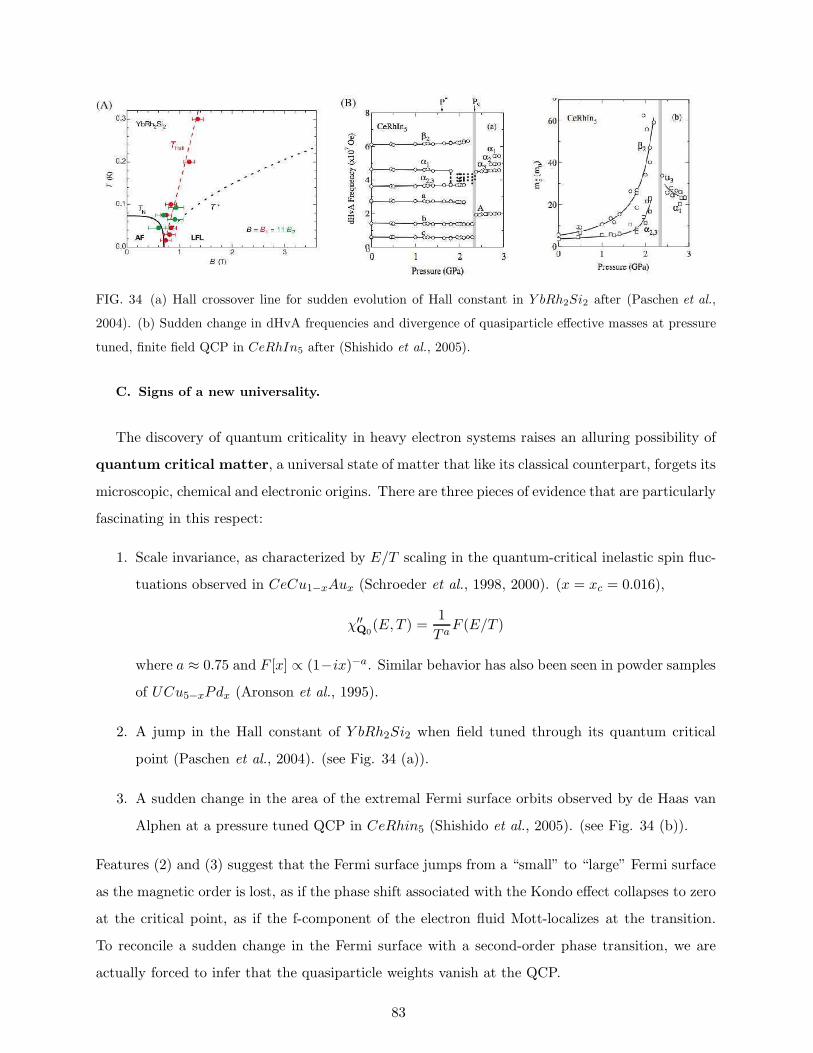
FIG. 34 (a) Hall crossover line for sudden evolution of Hall constant in Y bRh2Si2 after (Paschen et al.,
2004). (b) Sudden change in dHvA frequencies and divergence of quasiparticle effective masses at pressure
tuned, finite field QCP in CeRhIn5 after (Shishido et al., 2005).
C. Signs of a new universality.
The discovery of quantum criticality in heavy electron systems raises an alluring possibility of
quantum critical matter, a universal state of matter that like its classical counterpart, forgets its
microscopic, chemical and electronic origins. There are three pieces of evidence that are particularly
fascinating in this respect:
1. Scale invariance, as characterized by E/T scaling in the quantum-critical inelastic spin fluc-
tuations observed in CeCu1−xAux (Schroeder et al., 1998, 2000). (x = xc = 0.016),
χ′′Q0
(E,T ) =1
T aF (E/T )
where a ≈ 0.75 and F [x] ∝ (1−ix)−a. Similar behavior has also been seen in powder samples
of UCu5−xPdx (Aronson et al., 1995).
2. A jump in the Hall constant of Y bRh2Si2 when field tuned through its quantum critical
point (Paschen et al., 2004). (see Fig. 34 (a)).
3. A sudden change in the area of the extremal Fermi surface orbits observed by de Haas van
Alphen at a pressure tuned QCP in CeRhin5 (Shishido et al., 2005). (see Fig. 34 (b)).
Features (2) and (3) suggest that the Fermi surface jumps from a “small” to “large” Fermi surface
as the magnetic order is lost, as if the phase shift associated with the Kondo effect collapses to zero
at the critical point, as if the f-component of the electron fluid Mott-localizes at the transition.
To reconcile a sudden change in the Fermi surface with a second-order phase transition, we are
actually forced to infer that the quasiparticle weights vanish at the QCP.
83

These features are quite incompatible with a spin density wave QCP. In a spin density wave
scenario, the Fermi surface and Hall constant are expected to evolve continuously through a QCP.
Moreover, in an SDW description, the dynamical critical exponent is z = 2 so time counts as z = 2
dimensions in the scaling theory, and the effective dimensionality Deff = d+ 2 > 4 lies above the
upper critical dimension, where mean-field theory is applicable and scale invariant behavior is no
longer expected.
These observations have ignited a ferment of theoretical interest in the nature of heavy fermion
criticality. We conclude with a brief discussion of some of the competing ideas currently under
consideration.
1. Local quantum criticality
One of the intriguing observations (Schroeder et al., 1998) in CeCu6−xAux, is that the uniform
magnetic susceptibility, χ−1 ∼ T a + C, a = 0.75 displays the same powerlaw dependence on
temperature observed in the inelastic neutron scattering at the critical wavevector Q0. A more
detailed set of measurements by Schroeder et al. (Schroeder et al., 2000) revealed that the scale-
invariant component of the dynamical spin susceptibility appears to be momentum independent,
χ−1(q, E) = T a[Φ(E/T )] + χ−10 (q). (145)
This behavior suggests that the critical behavior associated with the heavy fermion QCP contains
some kind of local critical excitation (Coleman, 1999; Schroeder et al., 1998).
One possibility, is that this local critical excitation is the spin itself, so that (Coleman, 1999;
Sachdev and Ye, 1993; Sengupta, 2000)
〈S(τ)S(τ ′)〉 =1
(τ − τ ′)2−ǫ, (146)
is a power-law, but where ǫ 6= 0 signals non- Fermi liquid behavior. This is the basis of the “‘local
quantum criticality” theory developed by Si, Ingersent, Rabello and Smith (Si et al., 2001, 2003;
Smith and Si, 2000). This theory requires that the local spin susceptibility χloc =∑
q χ(q, ω)ω=0
diverges at a heavy fermion QCP. Using an extension of the methods of dynamical mean-field
theory (Georges et al., 1996; Kotliar et al., 2006), Si et al. find that it is possible to account for
the local scaling form of the dynamical susceptibility, obtaining exponents that are consistent with
the observed properties of CeCu6−xAux (Grempel and Si, 2003).
However, there are some significant difficulties with this theory. First, as a local theory, the
quantum critical fixed point of this model is expected to possess a finite zero-point entropy per spin,
84

a feature that is to date, inconsistent with thermodynamic measurements (Custers et al., 2003).
Second, the requirement of a divergence in the local spin susceptibility imposes the requirement
that the surrounding spin fluid behaves as layers of decoupled two dimensional spin fluids. By
expanding χ−10 (q) (145) about the critical wavevector Q, one finds that the singular temperature
dependence in the local susceptibility is given by
χloc(T ) ∼∫
ddq1
(q− Q)2 + Tα∼ T (d−2)α/2, (147)
requiring that d ≤ 2.
My sense, is that the validity of the original scaling by Schroeder et al still stands and that
these difficulties stem from a mis-identification of the critical local modes driving the scaling seen
by neutrons. One possibility, for example, is that the right soft variables are not spin per-se, but
the fluctuations of the phase shift associated with the Kondo effect. This might open up the way
to an alternative formulation of local criticality.
2. Quasiparticle fractionalization and deconfined criticality.
One of the competing sets of ideas under consideration at present, is the idea that in the
process of localizing into an ordered magnetic moment, the composite heavy electron breaks up
into constituent spin and charge components. Loosely speaking,
e−σ sσ + h− (148)
where sσ represents a neutral spin-1/2 excitation, or “spinon”. This has led to proposals
(Coleman et al., 2001; Pepin, 2005; Senthil et al., 2003) that gapless spinons develop at the quan-
tum critical point. This idea is faced with a conundrum, for even if free neutral spin-1/2 excitations
can exist at the QCP, they must surely be confined as one tunes away from this point, back into the
Fermi liquid. According to the model of “deconfined criticality” proposed by Senthil,Vishwanath,
Balent, Sachdev and Fisher (Senthil et al., 2004), the spinon confinement scale ξ2 introduces a sec-
ond diverging length scale to the phase transition, where ξ2 diverges more rapidly to infinity than
ξ1. One possible realization of this proposal is the quantum melting of two dimensional S = 1/2
Heisenberg antiferromagnet, where the smaller correlation length ξ1 is associated with the transi-
tion from antiferromagnet to spin liquid, and the second correlation length ξ2 is associated with
the confinement of spinons to form a valence bond solid (Fig. 35).
It is not yet clear how this scenario will play out for heavy electron systems. Senthil, Sachdev
and Vojta (Senthil et al., 2005) have proposed that in a heavy electron system, the intermediate
85

FIG. 35 “Deconfined criticality” (Senthil et al., 2004). The quantum critical droplet is defined by two
divergent length scales - ξ1 governing the spin correlation length, ξ2 on which the spinons confine, in the
case of the Heisenberg model, to form a valence bond solid.
spin liquid state may involve a Fermi surface of neutral (fermionic) spinons co-existing with a
small Fermi surface of conduction electrons which they call an FL∗ state. In this scenario, the
quantum critical point involves an instability of the heavy electron fluid to the FL∗ state, which is
subsequently unstable to antiferromagnetism. Recent work suggests that Hall constant can indeed
jump at such a transition (Coleman et al., 2005a).
3. Schwinger Bosons
A final approach to quantum criticality currently under development, attempts to forge a
kind of “spherical model” for the antiferromagnetic quantum critical point through the use of
a large N expansion in which the spin is described by Schwinger bosons, rather than fermions
(Arovas and Auerbach, 1988; Parcollet and Georges, 1997),
Sab = b†abb − δabnbN
where the spin S of the moment is determined by the constraint nb = 2S on the total num-
ber of bosons per site. Schwinger bosons are well-suited to describe low dimensional magnetism
(Arovas and Auerbach, 1988). However, unlike fermions, only one boson can enter a Kondo singlet.
To obtain an energy that grows with N , Parcollet and Georges proposed a new class of large N
expansion based around the multi-channel Kondo model with K channels (Parcollet and Georges,
1997), where k = K/N is kept fixed. The Kondo interaction takes the form
Hint =JKN
∑
ν=1,K, α, β
Sαβc†νβµcνα (149)
86

where the channel index ν runs from one to K. When written in terms of Schwinger bosons, this
interaction can be factorized in terms of a charged, but spinless exchange fermion χν (“holon”), as
follows
Hint →∑
να
1√N
[
(c†ναbα)χ†ν + H.c.
]
+∑
ν
χ†νχνJK
. (150)
Parcollet and Georges originally used this method to study the over-screened Kondo model
(Parcollet and Georges, 1997), where K > 2S.
Recently, it has proved possible to find the Fermi liquid large N solutions to the fully screened
Kondo impurity model, where the number of channels is commensurate with the number of bosons
(K = 2S) (Lebanon and Coleman, 2007; Rech et al., 2006). One of the intriguing features of these
solutions, is the presence of a gap for spinon excitations, roughly comparable with the Kondo tem-
perature. Once antiferromagnetic interactions are introduced, the spinons pair-condense, forming a
state with a large Fermi surface, but one that co-exists with gapped spinon (and holon) excitations
(Coleman et al., 2005b).
The gauge symmetry associated with these particles guarantees that if the gap for the spinon
goes to zero continuously, then the gap for the holon must also go to zero. This raises the possibility
that gapless charge degrees of freedom may develop at the very same time as magnetism (Fig. 36
). In the two impurity model, Rech et al have recently shown that the large N solution contains
a “Jones Varma” quantum critical point where a static valence bond forms between the Kondo
impurities. At this point, the holon and spinon excitations become gapless. Based on this result,
Lebanon and Coleman (Lebanon et al., 2006) have recently proposed that the holon spectrum may
become gapless at the magnetic quantum critical point (Fig. 36.) in three dimensions.
VI. CONCLUSIONS AND OPEN QUESTIONS
I shall end this chapter with a brief list of open questions in the theory of heavy fermions.
1. To what extent does the mass enhancement in heavy electron materials owe its size to the
vicinity to a nearby quantum phase transitions?
2. What is the microscopic origin of heavy fermion superconductivity and the in extreme cases
UBe13 and PuCoGa5 how does the pairing relate to both spin quenching and the Kondo
effect?
87

FIG. 36 Proposed phase diagram for the large N limit of the two impurity and Kondo lattice models.
Background- the two impurity model, showing contours of constant entropy as a function of temperature and
the ratio of the Kondo temperature to Heisenberg coupling constant, after (Rech et al., 2006). Foreground,
proposed phase diagram of the fully screened, multi-channel Kondo lattice, where S is the spin of the
impurity. At small S, there is a phase transition between a spin liquid and heavy electron phase. At large
S, a phase transition between the antiferromagnet and heavy electron phase. If this phase transition is
continuous in the large N limit, then both the spinon and holon gap are likely to close at the quantum
critical point (Lebanon et al., 2006).
3. What is the origin of the linear resistivity and the logarithmic divergence of the specific heat
at a “hard” heavy electron quantum critical point?
4. What happens to magnetic interactions in a Kondo insulator, and why do they appear to
vanish?
5. In what new ways can the physics of heavy electron systems be interfaced with the tremen-
dous current developments in mesoscopics? The Kondo effect is by now a well-established
feature of Coulomb blockaded quantum dots (Kouwenhoven and Glazman, 2001), but there
may be many other ways in which we can learn about local moment physics from mesoscopic
88

experiments. Is is possible, for example, to observe voltage driven quantum phase transitions
in a mesoscopic heavy electron wire? This is an area ripe with potential.
It should be evident that I believe there is tremendous prospect for concrete progress on many of
these issues in the near future. I hope that in some ways, I have whet your appetite enough to
encourage you too try your hand at their at their future solution.
Acknowledgments: This research was supported by the National Science Foundation grant
DMR-0312495. I’d like to thank E. Lebanon and T. Senthil for discussions related to this work.
I’d also like to thank the Aspen Center for Physics, where part of the work for this chapter was
carried out.
References
Abrikosov, A. A., 1965, Physics 2, 5.
Aeppli, G., and Z. Fisk, 1992, Comm. Condens. Matter Phys. 16, 155.
Aeppli, G., A. Goldman, G. Shirane, E. Bucher, and M.-C. Lux-Steiner, 1987, Phys. Rev. Lett. 58, 808.
Affleck, I., Z. Zou, T. Hsu, and P. W. Anderson, 88, Phys. Rev. B 8, 745.
Alekseev, P. A., E. S. Klement’ev, V. Lazukov, E. Nefedova, I. Sadikov, A. Y. Muzychka, I. L. Sashin, N. N.
Efremova, and W. Buhrer, 1994, JETP 79, 665.
Allen, J., S. Oh, O. Gunnarsson, K. Schonhammer, M. Maple, M. Torikachvili, and I. Lindau, 1986, Advances
in Physics 35, 275.
Allen, J. W., S. J. Oh, L. E. Cox, W. P. Ellis, S. Wire, Z. Fisk, J. L. Smith, B. B. Pate, I. Lindau, and
J. Arko, 1985, Phys. Rev. Lett. 2635, 54.
Allen, J. W., S. J. Oh, M. B. Maple, and M. S. Torikachvili, 1983, Phys. Rev. 28, 5347.
Anderson, P. W., 1961, Phys. Rev. 124, 41.
Anderson, P. W., 1970, J. Phys. C 3, 2346.
Anderson, P. W., 1973, Comm. S. St. Phys. 5, 72.
Anderson, P. W., 1981, in Valence Fluctuations in Solids, edited by L. M. Falicov and W. Hanke and M. P.
Maple (North Holland, Amsterdam), p. 451.
Anderson, P. W., 1987, Science 235, 1196.
Anderson, P. W., and G. Yuval, 1969, Phys. Rev. Lett. 45, 370.
Anderson, P. W., and G. Yuval, 1970, Phys. Rev. B 1, 1522.
Anderson, P. W., and G. Yuval, 1971, J. Phys. C 4, 607.
Andrei, N., K. Furuya, and J. Lowenstein, 1983, Rev. Mod. Phys 55.
Andres, K., J. Graebner, and H. R. Ott, 1975, Phys. Rev. Lett. 35, 1779.
Aoki, H., T. Sakahibara, H. Shishido, R. Settai, Y. Onuki, P. Maranovic, and K. Machida, 2004, J. Phys.
Condens. Matter 16, L13.
89

Aronson, M., R. Osborn, R. Robinson, J. Lynn, R. Chau, C. Seaman, and M. Maple, 1995, Phys. Rev. Lett.
75, 725.
Arovas, D., and A. Auerbach, 1988, Phys. Rev. B 38, 316.
Auerbach, A., and K. Levin, 1986, Phys. Rev. Lett. 57, 877.
Bang, Y., A. V. Balatsky, F. Wastin, and J. D. Thompson, 2004, Phys. Rev. 70, 104512.
Barnes, S. E., 1976, J. Phys. F 6, 1375.
Baskaran, G., Z. Zou, and P. W. Anderson, 1987, Sol. St. Commun 63, 973.
Bauer, E., G. H. H. Michor, C. Paul, E. W. Scheidt, A. Gribanov, Y. Seropegin, H. Nol, M. Sigrist, and
P. Rogl, 2004, Physical Review Letters 92, 027003.
Baym, G., and C. Pethick, 1992, Landau Fermi-Liquid Theory (Wiley, New York).
Berlin, T. H., and M. Kac, 1952, Phys. Rev. 86, 821.
Beyerman, W. P., G. Gruner, Y. Dlicheouch, and M. B. Maple, 1988, Phys. Rev. B 37, 10353.
Bishop, D. J., C. M. Varma, B. Batlogg, E. Bucher, Z. Fisk, and J. L. Smith, 1984, Phys. Rev. Lett. 53(10),
1009.
Blandin, A., and J. Friedel, 1958, J. Phys. Radium 19, 573.
Blount, E. I., C. M. Varma, and G. Aeppli, 1990, Phys. Rev. Lett 64, 3074.
Broholm, C., G. Aeppli, R. N. Kleiman, D. R. Harshman, D. J. Bishop, E. Bucher, D. L. Williams, E. J.
Ansaldo, and R. H. Heffner, 1990, Phys. Rev. Lett 65, 2062.
Bucher, B., Z. Schlessinger, P. C. Canfield, and Z. Fisk, 1994, Phys. Rev. Lett 72, 522.
Bucher, B., Z. Schlessinger, D. Mandrus, Z. Fisk, J. Sarrao, J. F. DiTusa, C. Oglesby, G. Aeppli, and
E. Bucher, 1995, Phys. Rev B 53, R2948.
Bucher, E., J. P. Maita, G. W. Hull, R. C. Fulton, and A. S. Cooper, 1975, Phys. Rev. B 11, 440.
Bud’ko, S. L., E. Morosan, and P. C. Canfield, 2004, Phys. Rev. B 69, 014415.
Bud’ko, S. L., V. Zapf, E. Morosan, and P. C. Canfield, 2005, Phys. Rev. B 72, 172413.
Bulla, R., 2006, Phil. Mag 86, 1877.
Burdin, S., A. Georges, and D. R. Grempel, 2000, Phys. Rev. Lett 85, 1048.
Cardy, J., 1996, Renormalization in Statistical Physics Cambridge University P (Cambridge).
Clogston, A. M., B. T. Mathias, M. Peter, H. J. Williams, E. Corenzwit, and R. C. Sherwood, 1962, Phys.
Rev. 125, 541.
Coleman, P., 1983, Phys. Rev. 28, 5255.
Coleman, P., 1984, Phys. Rev. 29, 3035.
Coleman, P., 1987a, Phys. Rev. B 35, 5072.
Coleman, P., 1987b, Phys. Rev. Lett. 59, 1026.
Coleman, P., 1999, Physica B 259-261, 353.
Coleman, P., and N. Andrei, 1989, J. Phys. Cond. Matt. C 1, 4057.
Coleman, P., J. B. Marston, and A. J. Schofield, 2005a, Phys. Rev. 72, 245111.
Coleman, P., I. Paul, and J. Rech, 2005b, Phys. Rev. B 72, 094430.
90

Coleman, P., C. Pepin, Q. Si, and R. Ramazashvili, 2001, J. Phys. Cond. Matt. 13, 273.
Coleman, P., A. M. Tsvelik, N. Andrei, and H. Y. Kee, 1999, Phys. Rev. B60, 3608.
Coqblin, B., and J. R. Schrieffer, 1969, Phys. Rev. 185, 847.
Cox, D., and N. Grewe, 1988, Zeit. fur Physik B 71, 273.
Cox, D., and M. Maple, 1995, Physics Today 482, 32.
Cox, D., and A. Zawadowski, 1999, Exotic Kondo effects in Metals (CRC Press, Boca Raton, Florida).
Curro, N. J., T. Caldwell, E. D. Bauer, L. A. Morales, M. J. Graf, Y. Bang, A. V. Balatsky, J. D. Thompson,
and J. L. Sarrao, 2005, Nature 434, 622.
Custers, J., P. Gegenwart, H. Wilhelm, K. Neumaier, Y. Tokiwa, O. Trovarelli, C. Geibel, F. Steglich,
C. Pepin, and P. Coleman, 2003, Nature 424, 524.
D, F., and M. Haldane, 1978, Phys. Rev. Lett 40, 416.
DeGiorgi, L., 1999, Rev. Mod. Phys. 71, 687.
Degiorgi, L., F.Anders, G. Gruner, and E. P. Society, 2001, Journal B 19, 167.
DiTusa, J. F., K. Friemelt, E. Bucher, G. Aeppli, and A. P. Ramirez, 1997, Phys. Rev. Lett. 831, 78.
Doniach, S., 1977, Physica B 91, 231.
Dordevic, S. V., D. N. Basov, N. R. Dilley, E. D. Bauer, and M. B. Maple, 2001, Phys. Rev. Lett. 86, 684.
Engelbrecht, J., and K. Bedell, 1995, Phys. Rev. Lett 74, 4265.
Estrela, P., A. de Visser, T. Naka, F. de Boer, and L. C. J. Pereira, 2002, Physica B 312-313, 482.
Fak, B., D. F. McMorro2, P. G. Niklowitz, S. Raymond, J. Floquet, P. C. Canfield, S. L. Budko, Y. Janssen,
and M. J. Gutmann, 2005, J. Phys. Cond. Matt. 17, 301.
Flouquet, J., 2005, “On the Heavy Fermion Road”, URL http://www.citebase.org/abstract?id=oai:arXiv.org:cond-ma
Fowler, M., and A. Zawadowskii, 1971, Solid State Commun 9, 471.
Fulde, P., J. Keller, and G. Zwicknagl, 1988, Solid State Physics 41, 1.
Gegenwart, P., J. Custers, Y. Tokiwa, C. Geibel, and F. Steglich, 2005, Phys. Rev. Lett 94, 076402.
Geibel, C., C. Schank, S. Thies, H. Kitazawa, C. D. Bredl, A. Bohm, M. Rau, A. Grauel, R. Caspary,
R. Hefrich, U. Ahlheim, G. Weber, et al., 1991, Zeit. Phys. B. 84, 1.
Geibel., C., S. Thies, D. Kacrowski, A. Mehner, A. Granel, B. Seidel, U. Ahnheim, R. Helfrich, K. Peters,
C. Bredl, and F. Steglich, 1991, Zeit. Phys. B. 83, 305.
Georges, A., and G. Kotliar, 1992, Phys. Rev. B 45, 6479.
Georges, A., G. Kotliar, W. Krauth, and M. Rozenberg, 1996, Rev. Mod. Phys. 6813.
Grempel, D. R., and Q. Si, 2003, Phys. Rev. Lett 91, 026401.
Grewe, N., and F. Steglich, 1991, in Handbook on the Physics and Chemistry of Rare Earths, edited by K.
A. Gschneider and L. Eyring (Elsevier, Amsterdam), volume 14, p. 343.
Grosche, F. M., P. Agarwal, S. R. Julian, N. J. Wilson, R. K. WHaselwimmer, S. J. S. Lister, N. D. Mathur,
F. V. Carter, S. S. Saxena, and G. GLonzarich, 2000, J. Phys. Cond. Matt. 12, L533.
Gruner, G., and A. Zawadowski, 1974, Rep. Prog. Phys 37, 1497.
Gunnarsson, O., and K. Schonhammer, 1983, Phys. Rev. B 28, 4315.
91

de Haas, de Boer, and D. van der Berg, 1933, Physica 1, 1115.
Hertz, J. A., 1976, Phys. Rev. B 14, 1165.
Hess, T. A. T. D. W., and J. A. Sauls, 1990, Phys. Rev. B 41, 8891.
Hewson, A. C., 1993, The Kondo Problem to Heavy Fermions (Cambridge University Press, Cambridge).
Hirsch, J. E., 1985, Phys. Rev. Lett 54, 1317.
Hundley, M. F., P. C. Canfield, J. D. Thompson, Z. Fisk, and J. M. Lawrence, 1990, Phys. Rev. B. 42, 6842.
Iga, F., M. Kasaya, and T. Kasuya, 1988, J. Magn. Magn. Mater. 76-77, 156.
Ikeda, H., and K. Miyake, 1996, J. Phys. Soc. Jpn. 65, 1769.
Isawa, K., Y. N. J. Goryo, Y. Matsuda, S. Osaki, H. Sugawara, H. Sato, P. Thalmeier, and K. Maki, 2003,
Phys. Rev. Lett. 90, 117001.
Izawa, K., T. Suzuki, T. Fujita, T. Takabatake, G. Nakamoto, H. Fujii, and K.Maezawa, 1999, Phys. Rev.
59, 2599.
Jaccarino, V., G. K. Wertheim, J. H. Wernick, C. R. Walker, and S. Arajs, 1967, Phys. Rev 160, 476.
Jarrell, M., 1995, Phys. Rev. B 51, 7429.
Jarrell, M., H. Pang, and D. L. Cox, 1997, Phys. Rev. Lett 78, 1996.
Jones, B., 2007, this volume.
Joynt, R., 1988, S. Sci. Techno . 1, 210.
Julian, S. R., P. A. A. Teunissen, and S. A. J. Wiegers, 1992, Phys. Rev. B 46, 9821.
Kadowaki, K., and S. Woods, 1986, Solid State Comm 58, 507.
Kagan, Y., K. Kikoin, and N. Prokof’ev, 1993, JETP Lett 57, 600.
Kasuya, T., 1956, Prog. Theo. Phys. 16, 45.
Kim, K. H., N. Harrison, M. Jaime, G. S. Boebinger, and J. A. Mydosh, 2003, Phys. Rev. Lett. 91, 256401.
Kimura, N., T. Komatsubara, D.Aoki, Y. Onuki, Y. Haga, E. Yamamoto, H. Aoki, and H. Harima, 1998, J.
Phys. Soc. Japan 67, 2185.
Kondo, J., 1962, Prof. Theo. Phys. 28, 772.
Kondo, J., 1964, Prog. Theo. Phys. 32, 37.
Kopp, A., and S. Chakravarty, 2005, Nature Phys. 1, 53.
Kotliar, G., 1988, Phys. Rev. B 37, 3664.
Kotliar, G., S. Y. Savrasov, K. Haule, V. S. Oudovenko, O. Parcollet, and C. A. Marianetti, 2006, Rev.
Mod. Phys 78, 865.
Kouwenhoven, L., and L. Glazman, 2001, Physics World 14, 33.
Kuchler, R., N. Oeschler, P. Gegenwart, T. Cichorek, K. Neumaier, O. Tegus, C. Geibel, J. A. Mydosh,
F. Steglich, and L. Zhu, 2003, Q. SiPhys. Rev. Lett 91, 066405.
Kuromoto, Y., and T. Watanabe, 1971, Physica B 148, 80.
Lacroix, C., and M. Cyrot, 1981, Phys. Rev. B 43, 12906.
Landau, L., 1957, Sov. Phys. JETP 3, 920.
Langer, J. S., and V. Ambegaokar, 1961, Phys. Rev. 121, 1090.
92

Langreth, D., 1966, Phys. Rev. 150, 516.
Lebanon, E., and P. Coleman, 2007, Fermi liquid identities for the Infinite U Anderson Model, Phys. Rev.
B (submitted), URL http://arxiv.org/abs/cond-mat/0610027.
Lebanon, E., J. Rech, P. Coleman, and O. Parcollet, 2006, Phys. Rev. Lett 97, 106604.
Lee, P. A., T. M. Rice, J. W. Serene, L. J. Sham, and J. W. Wilkins, 1986, Comments Condens. Matt. Phys.
12, 99.
Liu, L. Z., J. W. Allen, C. L. Seaman, M. B. Maple, Y. Dalichaouch, J. S. Kang, M. S. Torikachvili, and
M. A. L. de laTorre, 1992, Phys. Rev. Lett 68, 1034.
von Lohneysen, H., 1996, J. Phys. Cond. Mat. 8, 9689.
von Lohneysen, H., T. Pietrus, G. Portisch, H. G. Schlager, A. Schroeder, M. Sieck, and T. Trappmann,
1994, Phys. Rev. Lett. 72, 3262.
von Lohneysen, H., A. Rosch, M. Vojta, and P. Wolfe, 2007, Fermi-liquid instabilities at magnetic quantum
phase transitions, Rev Mod. Phys (submitted), URL http://arxiv.org/abs/cond-mat/0606317.
Luttinger, J. M., 1960, Phys. Rev. 119, 1153.
Luttinger, J. M., and J. C. Ward, 1960, Phys. Rev. 118, 1417.
Machida, K., and M. Ozaki, 1989, J. Phys. Soc. Japan 58, 2244.
Maple, B., W. Fertig, A. Mota, L. DeLong, D. Wohlleben, and R. Fitzgerald, 1972, Solid St. Commun 11,
829.
Martin, R. M., 1982, Phys. Rev. Lett. 48, 362.
Mathur, N., F. M. Grosche, S. R. Julian, I. R. Walker, D. M. Freye, and R. K. W. H. G. G. Lonzarich, 1998,
Nature 394, 39.
McCollam, A., S. R. Julian, P. M. C. Rourke, D. Aoki, and J. Flouquet, 2005, Phys. Rev. Lett. 94, 186401.
Meisner, G. P., M. S. Torikachvili, K. N. Yang, M. B. Maple, and R. P. Guertin, 1985, J. Appl. Phys. 57,
3073.
Mekata, M., S. Ito, N. Sato, T. Satoh, and N. Sato, 1986, Journal of Magnetism and Magnetic Materials
54, 433.
Menth, A., E. Buehler, and T. H. Geballe, 1969, Phys. Rev. Lett 22, 295.
Metzner, W., and D. Vollhardt, 1989, Phys. Rev. Lett. 62, 324.
Millis, A. J., P. A., and Lee, 1987a, Phys. Rev. B 35(7), 3394.
Millis, A. J., M. Lavagna, and P. A. Lee, 1987b, Phys. Rev. 36, 864867.
Miranda, E., and V. Dobrosavljevic, 2005, Rep. Prog. Phys 68, 2337.
Miyake, K., S. S. Rink, and C. M. Varma, 1986, Phys. Rev. B 34, 6554.
Monod, M. T. B., C. Bourbonnais, and V. Emery, 1986, Phys. Rev. B. 34, 7716.
Monthoux, P., and G. Lonzarich, 1999, Phys. Rev. B 59, 14598.
Moreno, J., and P. Coleman, 2000, Phys. Rev. Lett. 84, 342.
Moriya, T., and J. Kawabata, 1973, J. Phys. Soc. Japan 34, 639.
Nakamura, K., Y. Kitaoka, K. Asayama, T. Takabatake, H. Tanaka, and H. Fujii, 1994, J. Phys. Soc Japan
93

63, 433.
Nakasuji, S., D. Pines, and Z. Fisk, 2004, Two fluid description of the kondo lattice, Phys. Rev. Lett.
Niklowitz, P. G., G. Knebel, J. Flouquet, S. L. Bud’ko, and P. C. Canfield, 2006, Phys. Rev. B 73, 12501.
Norman, M., 2007, this volume ??
Norman, M. R., T. Oguchi, and A. J. Freeman, 1988, Phys. Rev. 38, 11193.
Nozieres, P., 1976, Journal de Physique C 37, 1.
Nozieres, P., 1985, Ann. Phys. Paris 10.
Nozieres, P., and A. Blandin, 1980, Journal de Physique 41, 193.
Nozieres, P., and J. M. Luttinger, 1962, Phys. Rev. 127, 1423.
Oguchi, T., and A. J. Freeman, 1985, J. Magn. Magn. Matter 52, 174.
Okiji, A., and N. Kawakami, 1983, Phys. Rev. Lett 50, 1157.
Onuki, Y., and T. Komatsubara, 1987, J. Mag. Mat. 63-64, 281.
Oshikawa, M., 2000, Phys. Rev. Lett. 84, 3370.
Ott, H. R., 1987, Prog. Low Temp Phys. 11, 215.
Ott, H. R., H. Rudigier, Z. Fisk, and J. L. Smith, 1983, Phys. Rev. Lett 50, 1595.
Ott, H. R., H. Rudigier, Z. Fisk, and J. L. Smith, 1985, in Proceedings of the NATO Advanced Study Institute
on Moment Formation in Solids, Vancouver Island, August 1983, Valence Fluctuations in Solids, edited
by W. J. L. Buyers (Plenum), p. 309.
Ott, H. R., H. Rudigier, T. M. Rice, K. Ueda, Z. Fisk, and J. L. Smith, 1984, Phys. Rev. Lett 52, 1915.
Paglione, J., M. A. Tanatar, D. G. Hawthorn, EBoaknin, R. W. Hill, F. Ronning, M. Sutherland, L. Taillefer,
C. Petrovic, and P. C. Canfield, 2003, Phys. Rev. Lett 91, 246405.
Paglione, J., M. A. Tanatar, D. G. Hawthorn, F. Ronning, R. W. Hill, M. Sutherland, L. Taillefer, and
C. Petrovic, 2006, Phys. Rev. Lett 97, 106606.
Palstra, T. T. M., A. A. Menovsky, J. van den Berg, A. J. Dirkmaat, P. H. Kes, G. J. Nieuwenhuys, and
J. A. Mydosh, 1985, Phys. Rev. Lett. 55, 2727.
Parcollet, O., and A. Georges, 1997, Phys. Rev. Lett. 79, 4665.
Paschen, S., T. Luhmann, S. Wirth, P. Gegenwart, O. Trovarelli, C. Geibel, F. Steglich, P. Coleman, and
Q. Si, 2004, Nature 432, 881.
Pepin, C., 2005, Phys. Rev. Lett. 94, 066402.
Petrovic, C., P. G. Pagliuso, M. F. Hundley, R. Movshovich, J. L. Sarrao, J. D. Thompson, Z. Fisk, and
P. Monthoux, 2001, J. Phys. Cond. Matt 13, L337.
Pitaevskii, L. P., 1960, Zh. Eksp. Teor. Fiz 37, 1794.
Puttika, W., and R. Joynt, 1988, Phys. Rev. B 37, 2377.
Ramakrishnan, T. V., 1981, in Valence Fluctuations in Solids, edited by L. M. Falicov and W. Hanke and
M. P. Maple (North Holland, Amsterdam), p. 13.
Read, N., and D. Newns, 1983a, J. Phys. C 16, 3274.
Read, N., and D. M. Newns, 1983b, J. Phys. C 29, L1055.
94

Read, N., and S. Sachdev, 1991, Phys. Rev. Lett 66, 1773.
Rech, J., P. Coleman, O. Parcollet, and G. Zarand, 2006, Phys. Rev. Lett 96, 016601.
Reinders, P. H. P., M. Springford, P. T. Coleridge, R. Boulet, and D. Ravot, 1986, Phys. Rev. Lett. 57,
1631.
Riseborough, P., 2000, Adv. Phys. 49, 257.
Ronning, F., C. Capan, E. D. Bauer, J. D. Thompson, J. L. Sarrao, and R. Movshovich, 2006, Phys. Rev.
73, 064519.
Rosch, A., 1999, Phys. Rev. Lett. 82, 4280.
Rozenberg, M. J., G. Kotliar, and H. Kajueter, 1996, Phys. Rev. B 54, 8451.
Ruderman, M. A., and C. Kittel, 1950, Phys. Rev 78, 275.
Sachdev, S., 2007, this volume this volume, ??
Sachdev, S., and J. Ye, 1993, Phys. Rev. Lett. 70, 3339.
Sarachik, M., E. Corenzwit, and L. D. Longinotti, 1964, Phys Rev. 135, A1041.
Sarrao, J. L., L. A. Morales, J. D. Thompson, B. L. Scott, G. R. Stewart, F. Wastlin, J. Rebizant, P. Boulet,
E. Colineau, and G. H. Lander, 2002, Nature 420, 297.
Sato, N., N. Aso, K. Miyake, R. Shiina, P. Thalmeier, G. Varelogiannis, C. Geibel, F. Steglich, and P. F. T.
Komatsubara, 2001, Nature 410 410, 340.
Scalapino, D. J., E. Loh, and J. E. Hirsch, 1986, Phys. Rev. B 34, 8190.
Schlessinger, Z., Z. Fisk, H. T. Zhang, and M. B. Maple, 1997, Physica B 237-238, 460.
Schrieffer, J. R., and P. Wolff, 1966, Phys. Rev. 149, 491.
Schroeder, A., G. Aeppli, E. Bucher, R. Ramazashvili, and P. Coleman, 1998, Phys. Rev. Lett. 80, 5623.
Schroeder, A., G. A. R. Coldea, M. Adams, O. Stockert, H. Lhneysen, E. Bucher, R. Ramazashvili, and
P. Coleman, 2000, Nature 407, 351.
Schweitzer, H., and G. Czycholl, 1991, Phys. Rev. Lett. 67, 3724.
Sengupta, A. M., 2000, Phys. Rev. 61, 4041.
Senthil, T., S. Sachdev, and M. Vojta, 2005, Physica B 359 361, 9.
Senthil, T., A. Vishwanath, L. Balents, S. Sachdev, and M. P. A. Fisher, 2004, Science 303, 1490.
Senthil, T., M. Vojta, S. Sachdev, and M. Vojta, 2003, Phys. Rev. Lett 90, 216403.
Shishido, H., R. Settai, H. Harima, and Y. Onuki, 2005, Journal of the Physical Society of Japa 74, 1103.
Si, Q., S. Rabello, K. Ingersent, and J. L. Smith, 2001, Nature 413, 804.
Si, Q., S. Rabello, K. Ingersent, and J. L. Smith, 2003, Phys. Rev. 68, 115103.
Sidorov, V. A., M. Nicklas, P. G. Pagliuso, J. L. Sarrao, Y. Bang, A. V. Balatsky, and J. D. Thompson,
2002, Phys. Rev. Lett 89, 157004.
Sigrist, M., and K. Ueda, 1991a, Rev. Mod. Phys. 63, 239.
Sigrist, M., and K. Ueda, 1991b, Rev. Mod. Phys 63, 239.
Smith, J. L., and P. S. Riseborough, 1985, J. Mag. Mat. 47-48, 545.
Smith, J. L., and Q. Si, 2000, Phys. Rev. 61, 5184.
95

Steglich, F., J. Aarts, C. D. Bredl, W. Leike, D. E. M. W. Franz, and H. Schafer, 1976, Phys. Rev. Lett 43,
1892.
Stewart, G., 1984, Rev. Mod. Phys 56, 755.
Stewart, G., 2001, Rev. Mod. Phys 73, 797.
Stewart, G., 2006, Rev. Mod. Phys. 78, 743.
Stewart, G. R., Z. Fisk, J. O. Willis, and J. L. Smith, 1984a, Phys. Rev. Lett 52, 697.
Stewart, G. R., Z. Fisk, and M. S. Wire, 1984b, Phys. Rev. 30, 482.
Suhl, H., 1965, Phys. Rev. 38A, 515.
Taillefer, L., and G. G. Lonzarich, 1988, Phys. Rev. Lett 60, 1570.
Taillefer, L., R. Newbury, G. G. Lonzarich, Z. Fisk, and J. L. Smith, 1987, J. Magn. Magn. Matter. 63-64,
372.
Takabatake, T., M. Nagasawa, H. Fujii, G. Kido, M. Nohara, S. Nishigori, T. Suzuki, T. Fujita, R. Helfrish,
U. Ahlheim, K. Fraas, C. Geibel, et al., 1992, Phys. Rev. 45, 5740.
Takabatake, T., H. Tanaka, Y. Bando, H. Fujii, S. Nishigori, T. Suzuki, T. Fujita, and G. Kido, 1994, Phys.
Rev. B 50, 623.
Takabatake, T., F. Teshima, H. Fujii, S. Nishigori, T. Suzuki, T. Fujita, Y. Yamaguchi, J. Sakurai, and
D. Jaccard, 1990, Phys. Rev. B 41, 9607.
Tanatar, M. A., J. Paglione, L. Taillefer, and C. Petrovic, 2006, Violation of a Universal Law at a Quantum
Critical Point, Nature (submitted).
Tou, H., Y. Kitaoka, K. Asayama, C. Geibel, C. Schank, and F. Steglich, 1995, J. Phys. Soc. Japan 64, 725.
Trovarelli, O., C.Geibel, S. Mederle, C. Langhammer, F. Grosche, P. Gegenwart, M. Lang, G. Sparn, and
F. Steglich, 2000, Phys. Rev. Lett. 85, 626.
Tsujji, H., H. Kontani, and K. Yoshimora, 2005, Phys. Rev. Lett 94, 057201.
Tsunetsugu, H., M. Sigrist, and K. Ueda, 1997, Rev. Mod. Phys. 69, 809.
Tsvelik, A., and P. Wiegman, 1983, Adv. Phys. 32, 453.
Varma, C., Z. Nussinov, and W. van Saarlos, 2002, Phys. Rep. 361, 267.
Varma, C. M., 1976, Rev. Mod. Phys. 48, 219.
Vekhter, I., P. Hirschfield, J. P. Carbotte, and E. J. Nicol, 1999, Phys. Rev. B 59, R9023.
Vidhyadhiraja, N. S., V. E. Smith, D. E. Logan, and H. R. Krishnamurthy, 2003, J. Phys. Cond. Matt 15,
4045.
Volovik, G. E., 1993, Sov. Phys. JETP Letters 58, 469.
Vorontsov, A., and I. Vekhter, 2006, Phys. Rev. Lett 96, 237001.
Wang, C. S., M. R. Norman, R. Albers, A. M. Boring, W. E. Pickett, H. Krakauer, and N. E. Christensen,
1987, Phys. Rev. 35, 7260.
White, R. H., and T. H. Geballe, 1979, in Solid State Physics, edited by H. Ehrenreich, F. Seitz, and
D. Turnbull (Academic Press, New York), volume 15, p. 283.
Wiegmann, P. B., 1980a, Phys. Lett. 80A, 163.
96

Wiegmann, P. B., 1980b, Phys. Lett. 80A, 163.
Wilson, K. G., 1976, Rev. Mod. Phys. 47, 773.
Witten, E., 1978, Nucl. Phys. B 145, 110.
Won, H., D. Parker, K. Maki, T. Watanabe, K. Izawa, and Y. Matsuda, 2004, Phys. Rev. B 70, 140509.
Yamada, K., 1975, Prog. Theor. Phys. 53, 970.
Yoshida, K., and K. Yamada, 1975, Prog. Theor. Phys. 53, 1286.
Yosida, K., 1957, Phys. Rev. 106, 896.
Young, A. P., 1975, Journal of Physics C Solid StatePhysics) 8, L309.
Yuan, H. Q., F. M. Grosche, M. Deppe, G. Sparn, C. Geibel, and F. Steglich, 2006, Phys. Rev. Lett. 96,
047008.
Zwicknagl, G., A. N. Yaresko, and P. Fulde, 2002, Phys. Rev. 65, 081103.
97