Acta Mech 229, 595–612 (2018)https://doi.org/10.1007/s00707-017-2042-x

ORIGINAL PAPER

C. R. Bocking · M. G. Blyth

Oxygen uptake and denitrification in soil aggregatesThis paper is dedicated to the memory of Franz Ziegler

Received: 16 February 2017 / Revised: 7 July 2017 / Published online: 15 November 2017© The Author(s) 2017. This article is an open access publication

Abstract A mathematical model of oxygen uptake by bacteria in agricultural soils is presented with the goalof predicting anaerobic regions in which denitrification occurs. In an environment with a plentiful supply ofoxygen, micro-organisms consume oxygen through normal respiration. When the local oxygen concentrationfalls below a threshold level, denitrification may take place leading to the release of nitrous oxide, a potentagent for global warming. A two-dimensional model is presented in which one or more circular soil aggregatesare located at a distance below the ground level at which the prevailing oxygen concentration is prescribed.The level of denitrification is estimated by computing the area of any anaerobic cores, which may developin the interior of the aggregates. The oxygen distribution throughout the model soil is calculated first foran aggregated soil for which the ratio of the oxygen diffusivities between an aggregate and its surround issmall via an asymptotic analysis. Second, the case of a non-aggregated soil featuring one or more microbialhotspots, forwhich the diffusion ratio is arbitrary, is examined numerically using the boundary-elementmethod.Calculations with multiple aggregates demonstrate a sheltering effect whereby some aggregates receive lessoxygen than their neighbours. In the case of an infinite regular triangular network representing an aggregatedsoil, it is shown that there is an optimal inter-aggregate spacing which minimises the total anaerobic core area.

1 Introduction

In a soil environment where the rate of uptake of oxygen through normal respiration is greater than the rateat which it is replaced from the atmosphere through diffusion, micro-organisms can instead generate energyfrom nitrate, NO−

3 . This process is known as anaerobic denitrification (for a review, see Knowles [19]). As aresult of denitrification, nitrate is converted to nitrogen gas, N2, via the sequence of steps (e.g. Smith et al.[30]):

NO−3 �⇒ NO−

2 �⇒ NO �⇒ N2O �⇒ N2. (1)

Nitrous oxide (N2O) is created at the penultimate step and may be released in that form without being furtherconverted into nitrogen gas. Nitrous oxide produced in this way may escape up through the ground surfaceand into the atmosphere, where it has a deleterious effect on stratospheric ozone and moreover poses a seriousthreat as a potent agent for global warming. The use of arable soils with a high nitrogen content, and thewidespread use of fertilisers, has exacerbated the problem. While the levels of nitrous oxide released fromsoils are much smaller than the wider levels of release of carbon dioxide into the atmosphere, and while thelatter is undoubtedly the most dangerous greenhouse gas, the warming potential of nitrous oxide is around 300times greater (Houghton et al. [16]). Smith [29] notes that approximately 65% of the emissions of nitrous oxideoriginate from soils (for a review of the processes governing the exchange of these and other gases between

C. R. Bocking · M. G. Blyth (B)School of Mathematics, University of East Anglia, Norwich, UKE-mail: m.blyth@uea.ac.uk

596 C. R. Bocking, M. G. Blyth

the soil and the atmosphere, see Smith et al. [30]). The notorious difficulty in measuring denitrification in thefield (e.g. Groffman et al. [14]) serves to underline the need for predictive theoretical models.

Simple one-dimensional models have been proposed to quantify oxygen uptake in soils and hence actas a predictor for levels of denitrification (see, for example, Kanwar [17], Leffelaar [21], Papendick andRunkles [24] and Radford and Greenwood [27]). Typically such models assume a constant surface-leveloxygen concentration at one end of the domain and include a no-flux boundary condition at the other endto represent an impermeable layer of rock at either finite or infinite depth. Greenwood [12] constructed amore sophisticated model in which an individual soil particle, hereinafter termed an aggregate, is exposed to aknown uniform oxygen concentration at its surface. The aggregate is assumed to be spherical and the oxygenprofile inside to be spherically symmetric. Denitrification occurs at points in the interior where the oxygenconcentration falls below a threshold level, whichGreenwood took to be zero. Thiswas assumed to occurwithina spherical-shaped region concentric with the aggregate boundary. Such a region is usually referred to as ananaerobic core. (We note in passing that very similar mathematical models have been constructed to study solidtumours—see, for example, Britton [4]). Greenwood and Berry [13] reported an error in Greenwood [12]’swork and extended the formulation to non-spherical aggregates. In reality, soil structure is highly complex (e.g.[9,15]), and while models have tended to assume some symmetry for mathematical simplicity, more complexmodels based on fractal geometry have attempted to capture the clustering, fragmentation and stability of realsoils (e.g. [25]). Models that cater for a cluster of aggregates, assuming a log-normal distribution of aggregatesize and a spherically symmetric profile within each aggregate, have been proposed by Smith [28] and Arahand Smith [2].

In the present work, we present a two-dimensional model of denitrification in soils, which determines theoxygen profile in a model soil comprising multiple aggregates by solving the diffusion and uptake problemsinside the aggregates and in the surround. The surface distribution of oxygen on each aggregate boundary is notknown in advance and depends on the location of the aggregate beneath the ground surface and its proximity toother aggregates.We consider solitary aggregates,multiple aggregates, aswell as extended networks containinga formally infinite number of individual aggregates. Oxygen is assumed to be consumed within each aggregateat a constant rate as a result of microbial action. Where the oxygen concentration falls below a prescribedlevel, an anaerobic core develops. The assumption of a constant uptake rate has also been adopted by a numberof previous workers on the grounds of mathematical simplicity (e.g. [7,12,24]). Kanwar [17] notes that thetake-up rate is likely to vary both with time and with depth. Radford and Greenwood [27] formulated theirone-dimensional oxygen distribution problemwith the uptake rate a function of the local oxygen concentration,although they assumed a constant rate in their calculations. Bocking [3] demonstrated that in the context ofthe two-dimensional problem to be studied in the present work, the latter assumption has little qualitativeeffect on the results and only a marginal quantitative effect. (A slightly larger anaerobic core is predicted in asingle aggregate for constant rate of uptake.) In keeping with previous models, and with established wisdom(e.g. Currie [7]), we assume that diffusion is the dominant mechanism controlling oxygen transport within thesoil and is in itself sufficient to explain the necessary gas interchange between the soil and the atmosphere(Keen [18]). By adopting a two-dimensional model, we aim to make some progress towards quantifying theeffect of soil structure, namely the distribution of aggregates within the soil, on anaerobic core volume withoutimporting the additional mathematical and computational complexity required by a fully three-dimensionalapproach.

Our study embraces two different viewpoints. In the first, we consider a so-called aggregated soil, whichis viewed as a network of individual soil aggregates surrounded by air, or in the case of a saturated soil, water.In the alternative viewpoint, the ground is filled with soil particles (so that there are no air or water pockets),but in some parts the take-up of oxygen is effectively negligible and elsewhere there are hot spots of microbialactivity causing substantial oxygen depletion (e.g. Kuzyakov and Blagodatskaya [20]). This is referred to as anon-aggregated soil (e.g. Montzka et al. [23]).

The layout of the paper is as follows: In the next section, we present our model problem for a singleaggregate. In Sect. 3, we present an asymptotic analysis for an aggregated soil on the assumption the diffu-sion ratio between the aggregate interior and the surround is small. In Sect. 4, the case of a non-aggregatedsoil is examined numerically using the boundary-element method. Finally, in Sect. 5 we summarise ourfindings.

Oxygen uptake and denitrification in soil aggregates 597

Fig. 1 A single soil aggregate, ormicrobial patch, with boundary A located beneath the ground level S and containing an anaerobiccore with boundary C . Oxygen diffuses throughout region 1 and diffuses and is consumed throughout region 2

2 Statement of the model

We consider the diffusion and consumption of oxygen within a two-dimensional soil aggregate located at adistance below ground level, as depicted in Fig. 1. We initially discuss the case of a single aggregate with acircular boundary A of radius a. The case of two or more aggregates will be considered in a later section.Referring to the set of Cartesian coordinates shown in Fig. 1, the surface of the soil (i.e. ground level), whichis designated boundary S, is located at y = 0, and the centre of the aggregate is located on the vertical axis aty = −h.

An anaerobic core develops inside the aggregate when the local oxygen concentration drops below athreshold level. The boundary of this anaerobic core is labelled C . The shape and location of the free boundaryC are unknown in advance and must be found as part of the solution to the problem. Although the shape ofC will be determined in the ensuing analysis, it is likely to be of secondary interest in practice; our principalconcern is to provide a framework for computing the anaerobic area enclosed by C to serve as a guide to theoverall level of denitrification.

Outside of the soil aggregate and below ground level, which we will henceforth refer to as region 1, weassume that oxygen diffuses freely with diffusivity D1 so that the local concentration, φ, satisfies Laplace’sequation, D1∇2φ = 0. The oxygen concentration at ground level is prescribed so that φ = φS , a constant, aty = 0. Far below the aggregatewe impose the conditionφy → 0 as y → −∞, so that the oxygen cannot escapedownwards. Physically, we envisage a layer of rock lying some way beneath the soil through which oxygencannot permeate. Inside the soil aggregate and outside the anaerobic core, which we will henceforth refer toas region 2, oxygen is assumed to diffuse while being consumed by bacteria at a constant rate. Accordinglythe local concentration, ψ , satisfies the Poisson equation D2∇2ψ = λ, where λ is the rate of consumptionand is subject to conditions of continuity of oxygen flux and oxygen concentration at the aggregate boundaryA. The consumption rate λ is assumed to be constant and independent of the local oxygen concentration. Atthe anaerobic core boundary C , we impose a condition of zero oxygen flux together with the requirementthat ψ = T , where T is the threshold value below which normal respiration ceases and denitrification occursinstead.

It is convenient to non-dimensionalise the problem using the aggregate radius a as the reference length andthe ground oxygen level φS as the reference concentration level. Accordingly, we obtain the dimensionlessproblem in region 1,

∇2φ = 0, (2)

with φ = 1 on S, and the continuity conditions on A,

φ = ψ, n · ∇φ = δ n · ∇ψ, (3)

598 C. R. Bocking, M. G. Blyth

where n is the unit normal to A pointing out of the aggregate, and also the condition that φy → 0 as y → −∞.In region 2, we have the dimensionless problem

∇2ψ = α, (4)

with

ψ = τ, n · ∇ψ = 0 (5)

on C , where n is the unit normal to C pointing outwards. The pertinent dimensionless parameters are

α = a2λ

φSD2, δ = D2

D1, τ = T

φS, H = h

a, (6)

where the last parameter provides a measure of how far the aggregate is beneath ground level.In general, the oxygen distribution around the boundary Awill be non-uniform, the exact variation depend-

ing on the location of the aggregate relative to the ground-level surface and to any other aggregates. Fixingpolar coordinates (r, θ) with origin at the centre of the aggregate, we suppose that the oxygen profile on theboundary is given by φ(1, θ) = Φ0 + Φ(θ), where Φ0 is a constant and Φ has zero mean. Assuming that theaggregate is aerobic throughout, the oxygen profile inside the aggregate is given by

ψ(r, θ) = 1

4α(r2 − 1) + Φ0 +

∞∑

n=1

rn(Φ(c)

n cos(nθ) + Φ(s)n sin(nθ)

), (7)

where the Φ(c,s)n are the Fourier coefficients of the boundary data on A. Evidently (7) is monotonic increasing

in r . An anaerobic core will therefore develop at the aggregate centre if

α > 4(Φ0 − τ), (8)

a condition which depends on the mean oxygen profile around the aggregate boundary and the thresholdparameter τ . Moreover, (8) underscores the physical importance of the parameter α as it essentially controlswhether or not denitrification occurs within the soil. It will be helpful to place this into a physical context.Numerical values for the physical parameters in the model which are relevant to real soils have been estimatedby various authors. In Table 1, we present typical values for rate of oxygen consumption, λ, the aggregatediffusivity D2, and the threshold concentration for denitrification T extracted from a number of sources in theliterature. The latter value is typically very small, and using the value due to Greenwood quoted in Table 1 wefind τ = 1.7 × 10−5. Consequently, we may reasonably assume that τ � 1. Based on a typical atmosphericoxygen concentration of 21%, we will assume the value φS = 0.21 for the surface-level oxygen concentration.We will also take the value for the diffusivity of oxygen in air, namely D1 = 0.2 cm2 s−1, as the referencevalue in region 1.

Since the diffusivity of oxygen in air is around ten thousand times the diffusivity of oxygen in water,selecting an appropriate value for δ depends crucially on the water content in the region around the aggregates,and we expect a sharp contrast in the diffusivity ratio for dry and for water-logged soils. For example, usingCurrie [8]’s estimates for D2 in the case of a water-saturated aggregate and a dry aggregate from Table 1, weobtain δ = 0.5× 10−5 and δ = 0.05, respectively. Using instead Greenwood [11]’s estimate for D2 quoted inTable 1 for a saturated aggregate, we obtain δ = 4.1 × 10−5.

Table 1 Typical physical parameter values

Parameter Source 1 Source 2 Source 3 Source 4

a 0.16 cm – 5.01 cm –λ 0.5 × 10−5 s−1 – 2 × 10−7 s−1 –D2 (A) 0.82 × 10−5 cm2 s−1 1.05 × 10−5 cm2 s−1 – 10−6 cm2 s−1

D2 (B) – – – 10−2 cm2 s−1

T 3 × 10−6 mol L−1 – – –

Source 1 refers to Greenwood [11,12], Source 2 is Radford and Greenwood [27], Source 3 is Smith [28] and Source 4 is Currie[8]. The quoted values of the internal aggregate diffusivity D2 are for (A) a water-saturated aggregate and (B) a dry aggregate

Oxygen uptake and denitrification in soil aggregates 599

Gardner [10], Allmaras et al. [1] and Smith [28] note that experiments based on aggregate sizes in Britishsoils and in US soils have shown that aggregate size follows a log-normal distribution. Using the data quotedfor curve (a) of figure 2 of Smith [28], we obtain an estimate for the mean aggregate size of 5.01 cm. Thisis the value quoted in Table 1. The smaller value of 0.16 cm obtained by Greenwood [11], and also quotedin Table 1, indicates the range of possible aggregate sizes, which may be found in different soils. Using themean value provided by Smith for our aggregate size a, and taking the oxygen consumption rate λ = 2×10−7

s−1 extracted from Smith [28] in Table 1 together with the value D2 = 10−6 cm2s−1 for a water-saturatedaggregate from Currie [8], we obtain the estimate α = 23.9. Using the smaller value of a = 0.16 providedby Greenwood [11], we obtain α = 0.02. It is clear, then, that quite a range of values of our dimensionlessparameter α is appropriate for a real soil.

It follows from the preceding discussion that for an aggregated soil comprising individual soil particlessurrounded by air, the diffusion ratio is very small, and this suggests that mathematical progress can be madeby seeking an asymptotic solution on this basis. This is examined in Sect. 3. For a non-aggregated soil, whichis a homogeneous soil that contains one or more compact regions of decaying organic matter, such as deadleaves for example, the diffusion ratio δ is expected to be of order unity. In this case, the solution to the problem(2)–(5), including the determination of the unknown boundaryC , must be found numerically. This is discussedin Sect. 4.

3 Aggregated soil model: small diffusion ratio

As discussed in the previous section, in the case of an essentially dry soil containingwater-saturated aggregates,the diffusion ratio δ is expected to be very small. Working on this assumption, in this section we seek anasymptotic solution to (2)–(5), which is valid for small δ. The remaining parameters in (6) are assumed to beO(1).

Assuming δ � 1, we expand the oxygen concentration in region 1 and region 2 by writing

φ = φ0(x, y) + δ φ1(x, y) + · · · , ψ = ψ0(x, y) + δ ψ1(x, y) + · · · . (9)

In region 1, the leading order concentration, φ0, satisfies Laplace’s equation with the conditions that φ0 = 1on y = 0, and φ0y → 0 as y → −∞ and n · ∇φ0 = 0 on A so that the aggregate behaves as if it has animpermeable boundary. The solution is given by φ0 = 1 everywhere in region 1. In region 2, the leading orderproblem is given by

∇2ψ0 = α, (10)

with ψ0 = 1 on A. The other two boundary conditions require that ψ0 = τ and n · ∇ψ0 = 0 on C , whoselocation is unknown. The symmetry of this problem suggests that to leading order C is a circle concentricwith A, of radius c0 say. Using polar coordinates (r, θ) with origin at the centre of the aggregate located at(x, y) = (0, −H), we find

ψ0 = 1

4α(r2 − 1) + 1 − 1

2αc20 log r, (11)

which satisfies the required Dirichlet condition at the outer boundary and the required Neumann condition atthe inner boundary, namely ψ0r (c0) = 0. The remaining Dirichlet condition at the inner boundary requires theanaerobic core radius c0 to satisfy the equation

τ − 1 − α

4(c20 − 1) + αc20

2log c0 = 0. (12)

It is straightforward to show that this equation is satisfied by a real value of c0 lying in the physical range0 ≤ c0 ≤ 1, provided that α > 4(1 − τ). We note that this condition coincides with (8) on substitutingΦ0 = 1 as for the present case. Hence if τ � 1, as stated above, then we essentially require that α > 4 forthe presence of an anaerobic core; if 0 ≤ α ≤ 4 the aggregate is aerobic throughout and no denitrificationoccurs. In Sect. 2, we obtained the physically realistic value α = 23.9, and evidently an anaerobic core willexist in this case. Returning to dimensional variables the requirement α > 4 is equivalent to a > 2

√φSD2/λ.

Using the values λ = 2 × 10−7 s−1 and D2 = 10−6 cm2 s−1 quoted in Table 1, together with φS = 0.21,we see that an aggregate will contain an anaerobic core if its radius exceeds 2.05 cm; otherwise, the rate of

600 C. R. Bocking, M. G. Blyth

4 8 12 16 20 24 282

3

4

5

6

7

8

(a)

4 8 12 16 20 24 280

0.2

0.4

0.6

0.8

1

(b)

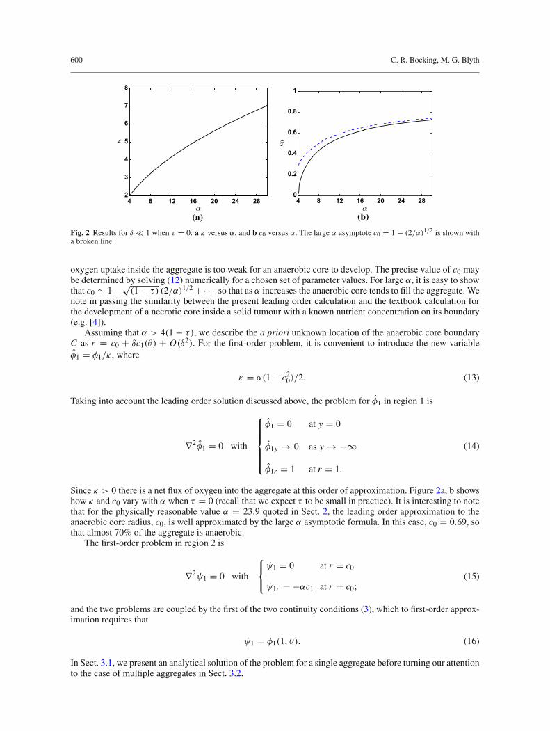
Fig. 2 Results for δ � 1 when τ = 0: a κ versus α, and b c0 versus α. The large α asymptote c0 = 1 − (2/α)1/2 is shown witha broken line

oxygen uptake inside the aggregate is too weak for an anaerobic core to develop. The precise value of c0 maybe determined by solving (12) numerically for a chosen set of parameter values. For large α, it is easy to showthat c0 ∼ 1−√

(1 − τ) (2/α)1/2 +· · · so that as α increases the anaerobic core tends to fill the aggregate. Wenote in passing the similarity between the present leading order calculation and the textbook calculation forthe development of a necrotic core inside a solid tumour with a known nutrient concentration on its boundary(e.g. [4]).

Assuming that α > 4(1 − τ), we describe the a priori unknown location of the anaerobic core boundaryC as r = c0 + δc1(θ) + O(δ2). For the first-order problem, it is convenient to introduce the new variableφ1 = φ1/κ , where

κ = α(1 − c20)/2. (13)

Taking into account the leading order solution discussed above, the problem for φ1 in region 1 is

∇2φ1 = 0 with

⎧⎪⎪⎪⎪⎨

⎪⎪⎪⎪⎩

φ1 = 0 at y = 0

φ1y → 0 as y → −∞

φ1r = 1 at r = 1.

(14)

Since κ > 0 there is a net flux of oxygen into the aggregate at this order of approximation. Figure 2a, b showshow κ and c0 vary with α when τ = 0 (recall that we expect τ to be small in practice). It is interesting to notethat for the physically reasonable value α = 23.9 quoted in Sect. 2, the leading order approximation to theanaerobic core radius, c0, is well approximated by the large α asymptotic formula. In this case, c0 = 0.69, sothat almost 70% of the aggregate is anaerobic.

The first-order problem in region 2 is

∇2ψ1 = 0 with

⎧⎨

⎩

ψ1 = 0 at r = c0

ψ1r = −αc1 at r = c0;(15)

and the two problems are coupled by the first of the two continuity conditions (3), which to first-order approx-imation requires that

ψ1 = φ1(1, θ). (16)

In Sect. 3.1, we present an analytical solution of the problem for a single aggregate before turning our attentionto the case of multiple aggregates in Sect. 3.2.

Oxygen uptake and denitrification in soil aggregates 601

3.1 Single aggregate

Before proceeding to consider a network of aggregates making up an aggregated soil, it is of interest to examinethe case of a single aggregate in isolation and to determine its effect on the ambient oxygen distribution. Thefirst-order problem in region 1, namely (14), may be tackled by introducing an image aggregate above theground surface and then employing bipolar coordinates (see Bocking [3] for details). An appealing alternativeis to introduce an image aggregate as described and then to make use of the Villat formula from potentialtheory, which is applicable to problems with doubly-connected domains (e.g. [5,6]). Following the latter path,and writing z = x + iy, we seek a representation via a complex function,

w(z) = φ1(x, y) + iv(x, y), (17)

which is analytic in the region exterior to A and its image region AI , obtained by reflecting A in the x axis.Furthermore, we demand that

v = Im(w) =⎧⎨

⎩

−s on A,

s on AI ,(18)

where s denotes arc length around the boundary of either A or AI , measured in the counterclockwise directionwith s = 0 at the lowermost point. Condition (18) has been derived by using the Cauchy–Riemann equationsto recast the Neumann boundary condition on A in (14) and its counterpart on the image aggregate AI . Usingthe terminology of fluid mechanics, according to (18) the aggregate is endowed with a nonzero circulationand this must be properly accounted for in the solution. Proceeding, we transform the physical domain in thez-plane to the annulus ρ < |ζ | < 1 in the ζ -plane via the conformal mapping

ζ = ρ1/2(A + iz

A − iz

), with A2 = H2 − 1, ρ = H − A

H + A , (19)

and define W (ζ ) ≡ w(z). Under mapping (19), the circles A′ at |ζ | = 1 and A′I at |ζ | = ρ are the ζ -plane

images of the circles A and AI , respectively.We seek a solution in the annular region ρ < |ζ | < 1 in the form

− iW (ζ ) = i log(ζ/ρ1/2) − ig(ζ ), (20)

where g(ζ ) is analytic in the annulus. Again using the terminology of fluid mechanics, we may interpret thefirst term in (20) as representing a point vortex of one sign located at z = −A i (inside A) and a point vortex ofthe opposite sign located at z = A i (inside AI ) in the z-plane. In this way, each of the aggregates is furnishedwith the necessary circulation alluded to above. To complete a solution which fulfils the boundary conditions(18), the analytic function g(ζ ) must be such that its real part satisfies

Re(−ig) =⎧⎨

⎩

(θ − s) on |ζ | = 1,

(θ − s) on |ζ | = ρ,

(21)

where θ is the polar angle in the ζ plane, with θ = 0 on the real ζ axis. Notice that mapping (19) switchesthe direction of transit around A from counterclockwise in the z-plane to clockwise in the ζ -plane and thisaccounts for the first terms on the right-hand sides of (21) being of the same sign on each of the two ζ -imagecircles. The problem to find the analytic function g is of the modified Schwarz type: it demands a single-valuedanalytic function whose real part satisfies a prescribed condition on the domain boundary.

Using the Villat formula (e.g. Crowdy et al. [5], Crowdy [6]), the solution is given by

− ig(ζ ) = I+(ζ ) − I−(ζ ) + Ic + ig0, (22)

where g0 is a constant and

I+(ζ ) = 1

2π i

∫

|ζ ′|=1K (ζ/ζ ′) (θ − s)

dζ ′

ζ ′ , I−(ζ ) = 1

2π i

∫

|ζ ′|=ρ

K (ζ/ζ ′) (θ − s)dζ ′

ζ ′ ,

(23)

Ic = − 1

2π i

∫

|ζ ′|=1(θ − s)

dζ ′

ζ ′ ,

602 C. R. Bocking, M. G. Blyth

where

K (ζ ) = 1 − 2ζ

Q(ζ )

dQ

dζ, Q(ζ ) = (1 − ζ )

∞∏

k=1

(1 − ρ2kζ )(1 − ρ2kζ−1). (24)

The arc distance around each circle needed in (23) may be computed using the formula

s =∫ θ

−π

|ζ z′(ζ )| dθ . (25)

When ζ lies on either of the circles so that ζ = ζ ′ at some point in the range of integration in either I+ or I−, therespective integral is to be interpreted in the Cauchy principal value sense. We also note that the compatibilitycondition for single valuedness, equation (6) in [5], is satisfied. The solution to the φ1 problem is obtained bytaking the real part of w and choosing the constant g0 = 0 so that φ1 = 0 on y = 0. Independent confirmationof this solution has been obtained by checking first against the solution obtained using bipolar coordinates andsecond against a numerical solution obtained using the boundary-element method (see Bocking [3]).

Next we seek a solution to the first-order interior problem (15). Since the right-hand side of the continuitycondition (16) is a periodic function, we may express it as a Fourier series and seek a solution to the unknowncore boundary correction c1(θ) in the same form. Using the fact that the problem is symmetric about thevertical line x = 0 passing through the aggregate centre, we may write the solution to the first-order exteriorproblem in the form

φ1(1, θ) = κμ0 + κ

∞∑

n=1

μn sin(nθ), μ0 = 1

2π

∫ 2π

0φ1(1, θ) dθ, (26)

where μ0 is the mean value of φ1 on the boundary. We seek a solution to the interior problem (15) in the form

ψ1 = A log r + B +∞∑

n=1

(Cnrn + Dnr

−n) sin(nθ), c1(θ) = ν0 +∞∑

n=1

νn sin(nθ), (27)

where the constants A, B, Cn , Dn and the coefficients νn are to be determined. Of particular interest are thevalues νn , which determine the first-order correction c1 to the anaerobic core radius. These are found to be

ν0 = κμ0

αc0 log c0, νn = 2nκ

αc0(cn0 − c−n0 )

μn (n = 0). (28)

To leading order the region exterior to the aggregate (region 1) is perfused with oxygen at the sameconcentration level as at the ground surface, so that φ0 = 1. Although the leading order oxygen distributionis uniform, the positioning of the aggregate inside region 1 is important. Intuitively, we expect the anaerobiccore to be larger the deeper the aggregate is located underground. In the present analysis, the area A of theanaerobic core inside the aggregate is given by

A = πc20 +(

πμ0(1 − c20)

log c0

)δ + O(δ2). (29)

The first term corresponds to the anaerobic core area for an aggregate in an infinite surround with a uni-form oxygen concentration. By considering the following identity for the harmonic function φ1, namely∇ · (φ1∇φ1) = |∇φ1|2, and integrating over the domain of region 1 and applying the divergence theorem, weobtain

μ0 = − 1

2π

∫

A|∇φ1|2 dl < 0, (30)

where l measures arc length around the boundary, and so the mean oxygen concentration around the aggregateperimeter A is negative. Therefore, since 0 < c0 < 1, the second term in (29) is positive and the area of theanaerobic core is increased from its value in an infinite surround.

Figure 3a shows the variation of μ0 with depth H . The large-depth behaviour can be determined byrecognising that when the aggregate is a long way below ground level, it can be represented by a point sink of

Oxygen uptake and denitrification in soil aggregates 603

0 1 2 3 4 5-2.5

-2

-1.5

-1

-0.5

0

(a)

4 8 12 16 20 24 280

0.2

0.4

0.6

0.8

1

(b)

Fig. 3 Results for δ � 1 when τ = 0: a the dependence ofμ0 on dimensionless depth H . The result using the exact Villat formulais shown with a solid line, and the approximate result μ0 = − log(2H) is shown with a dashed line. b The scaled anaerobic coreareaA/π according to (29) for depths H = − 1.00, − 3.21, − 5.42, − 7.63 (H increasing in the direction of the arrow as shown)for δ = 0.05 (solid lines) and δ = 0.1 (broken lines)

oxygen located at its centre x0 = (x0, −H) such that φ1(x) = κ log(r/R), where x = (x, y), r = |x − x0|,R = |x − x′

0|, and x′0 = (x0, H) is the location of an image source above ground level. The dashed line in

Fig. 3a represents the valueμ0 = − log(2H), which is calculated by substituting the point sink approximationfor φ1 = φ1/κ into the second equation in (26). The approximate result qualitatively reproduces the truebehaviour over the whole range and quantitatively agrees closely with the correct value from a depth of onlya few aggregate radii. The anaerobic core area scaled by the area of the aggregate, A/π , is shown in Fig. 3bplotted against α. The area is calculated using formula (29) neglecting the term O(δ2) and is shown for asequence of dimensionless depths H and for two different small values of δ. Evidently, the core area increaseswith depth, as anticipated.

3.2 Multiple aggregates

We now extend our discussion to describe an aggregated soilmodelled as an organised network ofM aggregateseach with a circular boundary of unit dimensionless radius. The primary difficulty lies in determining thesolution to the exterior problem in region 1. Here the first-order problem is given by (14) with the Neumannboundary condition represented by the last condition in (14) to be applied at each of the aggregate boundaries.We obtain the solution numerically using the boundary-element method. Following an established procedurefor the Laplace equation (e.g. [26]), we first reformulate the problem for φ1 as the integral equation of thesecond kind,

1

2φ1(x0) = −κ

∫

AG(1)(x, x0) dl(x) +

∫

An · ∇G(1)(x, x0) φ1(x) dl(x), (31)

where the point x0 lies on A, which now represents the union of all of the individual aggregate boundaries. TheGreen’s function is taken to beG(1)(x, x0) = (1/2π) log(r/R), where r = |x−x0| = [(x−x0)2+(y−y0)2]1/2and R = [(x − x0)2 + (y + y0)2]1/2; note that G(1) vanishes on y = 0.

The integral equation (31) is solved numerically by first discretizing each of the aggregate boundariescomprising A using a sequence of N straight-line boundary elements alongwhich φ1 is assumed to be constant.Enforcing (31) at the mid-point of each of these elements, and approximating the integrals using Gauss–Legendre quadrature, we obtain a set of NM algebraic equations for the NM unknown constant values of φ1on the elements. The linear system of equations is solved using Gaussian elimination. In implementing thisprocedure, we employed codes made freely available in the BEMLIB library [26]. In the results to be discussedbelow N was taken to be sufficiently large (typically between 100 and 200) to ensure that results are correct tothe quoted number of decimal places. Once the exterior problem is solved, the analysis for the interior problemcorresponding to (15) in each of the aggregates is similar to that presented above, and the same expression forarea (29) applies with μ0 representing the mean value of φ1/κ on the boundary of the aggregate in question,this value being available from the numerical solution of the exterior problem.

604 C. R. Bocking, M. G. Blyth

H

1β

1

2

d

d

3

β

(a)

0 0.1 0.2 0.3 0.4 0.5-3.6

-3.4

-3.2

-3

-2.8

-2.6

-2.4

-2.2

-2

1

2

(b)

0 0.1 0.2 0.3 0.4 0.5

-5

-4.5

-4

-3.5

-3

-2.51

3

2

(c)

0 0.1 0.2 0.3 0.4 0.5-7.5-7

-6.5-6

-5.5-5

-4.5-4

-3.5-3

-2.5

1

2

43

(d)

Fig. 4 Multi-aggregate case for δ � 1: a Illustrative sketch of three congruent aggregates separated by a dimensionless distanced at an angle β. The first aggregate has centre at dimensionless depth H . Panels (b–d) show the mean value μ0 when b twoaggregates are present, c three aggregates are present, and d four aggregates are present, each for varying orientation angle β/πwith d = 3 and H = 2. In each case, the curve labels refer to the aggregate number, which follows the convention illustrated inpanel (a)

It is of interest to discuss how the number and relative arrangement of aggregates affect the mean valueμ0. Consider a number of aggregates whose centres are located on a straight line inclined at an angle β to thehorizontal and separated by a dimensionless distance d . The centre of the first aggregate, being the uppermost,is located at a dimensionless depth H below the ground level. Figure 4a illustrates the envisaged scenario inthe case of three aggregates. Calculations were made for two aggregates, three aggregates and four aggregates.Figure 4b shows the mean value μ0 for the two aggregate case, M = 2, over a range of orientation angles βand for fixed aggregate separation d = 3. Note for comparison that if the second aggregate is removed so thatonly the uppermost aggregate remains, then we find μ0 = −1.5. We observe in Fig. 4b that the value of |μ0|for both aggregates exceeds this value for a single aggregate. If d is increased, the value of μ0 for aggregate1 tends towards the value for a solitary aggregate, μ0 = −1.5, as might be expected. When β = 0, the samemean value μ0 = −2.2 is computed for both aggregates. As the second aggregate moves beneath the first, itfeels a sheltering effect which accords with intuition. In particular, as the inclination angle β reaches π/2 theanaerobic core in aggregate 2 is significantly larger than that in aggregate 1.

Results for the same scenario but now with three aggregates (M = 3) or four aggregates (M = 4) areshown in panels (c) and (d) of the same figure. The mean valueμ0 decreases monotonically with β in all cases,and so the configuration for which the total anaerobic core area (summed over the aggregates) is maximisedoccurs when the aggregates are vertically aligned with β = π/2, as would be expected. For the three-aggregatecase shown in Fig. 4c, two features are particularly striking. First, the differential in the value of μ0 betweenaggregates 1 and 2, for example, is much greater in the vertical alignment than in the horizontal alignment.Second, in the vertical alignment themiddle aggregate (2) has a larger anaerobic core than the bottom aggregate(3). For the case of four aggregates shown in Fig. 4d, we see that when in the horizontal alignment (β = 0),

Oxygen uptake and denitrification in soil aggregates 605

D

H L

χ

(a)

0 0.5 1 1.5 2 2.5-28

-27.5

-27

0 0.5 1 1.5 2 2.5-70

-65

-60

0 0.5 1 1.5 2 2.5-85

-80

(b)

Fig. 5 Multi-aggregate case for δ � 1: a Sketch of a dislocated rectangular periodic lattice of aggregates located at a dimensionlessdistance H below ground with vertical row spacing D, and with one row shifted to the right by an amount 0 ≤ χ ≤ L . b Themean value μ0 for the array in panel (a) with H = 1.5, L = 2.5 and D = (

√3/2)L = 2.17. The middle or bottom row (solid or

dashed line, respectively) is shifted horizontally by χ . The value of μ0 on one aggregate in the upper/middle/lower row is shownin the upper/middle/lower panel

the anaerobic core sizes for aggregates 1 and 4 are the same and those for aggregates 2 and 3 are the same,and moreover, the latter exceed the former. Evidently the innermost aggregates are sheltered by the outermostaggregates and receive less oxygen. Curiously, the anaerobic core size for aggregate 4 is larger than that foraggregate 2 when β ≈ 0.3, but remains smaller than that for aggregate 3 even up to β = π/2. Consequently,for four aggregates in the vertically aligned position, the third aggregate down feels the greatest shelteringeffect and receives the least oxygen.

An infinite network made up of a periodic repetition of an individual cluster of M aggregates provides amore realistic model of an aggregated soil. The periodic extension in the horizontal direction of the scenariojust discussed is illustrated in Fig. 5a. The calculations for M aggregates in this periodically extended networkare readily made by replacing G(1) with the singly periodic Green’s function,

G(3) = 1

4πlog

{2 cosh

[k(y + y0)

] − 2 cos[k(x − x0)

]}

− 1

4πlog

{2 cosh

[k(y − y0)

] − 2 cos[k(x − x0)

]}, (32)

where k = 2π/L and L is the period. This function has been constructed so that G(3) = 0 on y = 0. It hasthe property limy→−∞ G(3) = constant. Figure 5b shows calculated values of μ0 for three rows of circularaggregates forming a rectangular lattice with periodicity L = 2.5. The first row is a dimensionless distanceH = 1.5 below ground level, and the rows are separated by a vertical distance D = (

√3/2)L = 2.17

dimensionless units. Either the middle or the bottom row suffers a dislocation in which one of the rows isshifted through a horizontal distance χ , where 0 < χ < L . For χ = 0, we have a regular rectangular lattice.Evidently the largest anaerobic cores are obtained when χ = L/2, and the optimal state (under the statedconditions) in which the total anaerobic core area is maximised is obtained when the aggregates are equallyspaced with their centres at the intersections of a uniform equilateral triangular network, corresponding toχ = L/2. Investigating this equitriangular network further, we show in Fig. 6 how μ0 depends on the networkspacing L . Note that when L = 2.5 the network corresponds to that shown in Fig. 5a for χ = L/2. The resultspredict that the anaerobic core size in each aggregate will increase sharply as the network spacing is reducedand the aggregates become tightly packed. As the network spacing is increased, the mean value μ0 for the firstparticle increases monotonically and eventually approaches the relevant value for an isolated aggregated at theappropriate depth (see Fig. 3a) as L → ∞. This value is shown with a broken line in the figure. Interestingly,we see that for aggregates 2 and 3 the curves have a maximum so that there is an optimal spacing to minimisethe size of the anaerobic cores in the second and the third rows of the network. Note that the maxima occurat similar, but not equal, values of L: for the case shown in the figure the maxima are at L = 35.8 for row 2and L = 37.6 for row 3. We note that adding more rows to the network gives qualitatively similar results. For

606 C. R. Bocking, M. G. Blyth

20 40 60 80 100 120 140

-25

-20

-15

-10

-5

0

1

2

3

Fig. 6 Multi-aggregate case for δ � 1: The mean value μ0 for a uniform triangular network with the aggregate centres equallyspaced by an amount L , and the uppermost row placed at a depth H = 1.5. The curves 1, 2, 3 correspond to values of μ0 on theaggregates labelled by the same numbers in Fig. 5a. The asymptote μ0 = − 2.411 for a solitary particle is shown with a brokenline

example, including a fourth row we find results similar to those in Fig. 6 with an additional curve for aggregate4 which is qualitatively similar to those for aggregates 2 and 3 and lying beneath both of them.

4 Non-aggregated soil: arbitrary diffusion ratio

For arbitrary values of the diffusion ratio δ, we compute the solution to problem (2)–(5) numerically usingthe boundary-element method. First we reformulate the problem as a set of coupled integral equations. Theformulation for the Laplace equation in region 1 is standard (e.g. Pozrikidis [26]). Introducing the new variableφ = φ − 1, in region 1 and following the usual procedure, we obtain

1

2φ(x0) = −

∫

AG(1)(x, x0) n · ∇φ(x) dl(x) +

∫

An · ∇G(1)(x, x0) φ(x) dl(x), (33)

where x0 lies on A, and n is the unit normal to A pointing into region 1. The Green’s function G(1)(x, x0) wasdefined in the previous section.

To develop a similar integral formulation for the Poisson equation (4) in region 2, we start with Green’ssecond identity and integrate over region 2, denoted here by Ω , to obtain

ψ(x0) = −∫

A,CG(2)(x, x0) n · ∇ψ(x) dl(x) +

∫

A,Cψ(x) n · ∇G(2)(x, x0) dl(x)

− α

∫∫

Ω

G(2)(x, x0) dx dy, (34)

where n is the unit normal to A or C pointing into region 2 in either case, and G(2)(x, x0) = (1/2π) log r isthe free-space Green’s function with r = |x − x0|. To recast the area integral in (34) as an integral around thedomain boundary, we make use of Green’s theorem in the plane for a domain Ω with boundary ∂Ω ,

∮

∂Ω

(L dx + M dy) =∫∫

Ω

(Mx − Ly) dx dy, (35)

and choose

L(x, y) = − 1

8π

(y − 2 y log r

), M(x, y) = 1

8π

(x − 2x log r

), (36)

Oxygen uptake and denitrification in soil aggregates 607

where x = x − x0 and y = y − y0, in order that Mx − Ly = G(2). Accordingly, we obtain a pair of integralequations in region 2 involving only integrals over the domain boundary. Writing a = (L , M), we have

1

2(φ(x0) + 1) = − 1

δ

∫

AG(2) n · ∇φ(x) dl(x) +

∫ PV

A(φ(x) + 1) n · ∇G(2) dl(x) − α

∫

Aa · t dl(x)

−∫

CG(2) n · ∇ψ(x) dl(x) + τ

∫

Cn · ∇G(2) dl(x) + α

∫

Ca · t dl(x), (37)

valid when x0 is on A, and

1

2τ = − 1

δ

∫

AG(2) n · ∇φ(x) dl(x) +

∫

A(φ(x) + 1) n · ∇G(2) dl(x) − α

∫

Aa · t dl(x)

−∫

CG(2) n · ∇ψ(x) dl(x) + τ

∫ PV

Cn · ∇G(2) dl(x) + α

∫

Ca · t dl(x), (38)

valid when x0 is on C . The superscript PV indicates that an integral should be interpreted in the Cauchyprincipal value sense. The unit tangent vector t points in the direction of increasing arc length l along a givenboundary. We have made use of the continuity conditions (3) in deriving (37) and (38).

Our goal is to solve (33) together with (37) and (38) to determine the boundary concentration levels of φand ψ and to determine the shape and location of the unknown anaerobic core boundary C . To accomplishthis, we first guess the location of C and discretise the individual integrals using straight-edged boundaryelements, taking N elements each around A and C . Imposing each of the integral equations at the mid-pointsof the elements, we obtain 3N linear algebraic equations for 3N unknowns including φ and n · ∇φ at theelement mid-points on A, and n ·∇ψ at the element mid-points onC . The equations are solved using Gaussianelimination. Once we have solved the linear system, we update the location of C to enforce the zero fluxboundary condition. To do this, we perturb the location of each of the nodes at the joins of the boundaryelements in turn by moving the node a small increment in the direction of the local outward normal vector.We then resolve the above system of integral equations for the perturbed core boundary and then iterate usingNewton’s method until n · ∇ψ at each node is less than a prescribed tolerance.

Once we have solved the integral equations and determined the position and shape of C , we may find theoxygen concentration at any point in the interior of region 1 and region 2 using the expressions

φ(x0) = −∫

AG(1) n · ∇φ(x) dl(x) +

∫

Aφ n · ∇G(1) dl(x), (39)

for x0 in the region 1, and

ψ(x0) = −∫

AG(2) n · ∇ψ dl(x) +

∫

Aψ(x) n · ∇G(2) dl(x) − α

∫

Aa · t dl(x)

−∫

CG(2)n · ∇ψ(x) dl(x) + τ

∫

Cn · ∇G(2)dl(x) + α

∫

Ca · t dl(x) (40)

for x0 in region 2.The preceding formulation is easily adapted to cater for multiple regions of oxygen-absorbing soil, and

the case of more than one microbial hot spot will be considered below an aggregated soil. Physically relevantvalues of the dimensionless parameters are discussed in Sect. 2. Here we assume a small patch of microbialactivity with the oxygen diffusivities taken to be broadly the same in both the interior and the exterior of thepatch. Therefore, we consider a range of values for δ but with a focus on the case δ = 1. Since, as discussedin Sect. 3, the critical oxygen level for denitrification to occur is very small, so that τ � 1, for computationalpurposes we simply set τ = 0 throughout the remainder of this section.

4.1 Results

We present numerical results computed using the boundary-element method for arbitrary values of δ. Accord-ingly, we assume that the whole of the underground domain y < 0 is densely occupied with soil and thatoxygen depletion occurs through high microbial activity in isolated regions which is much more significant

608 C. R. Bocking, M. G. Blyth

0 0.2 0.4 0.6 0.8 10.5

1

1.5

2

2.5

3

3.5

Fig. 7 Dependence of the threshold value of α for the appearance of an anaerobic core on the diffusion ratio, δ, for the case τ = 0and H = 4. An anaerobic core is present when α > αc

-2 -1 0 1 2-6

-5

-4

-3

-2

-1

0

C

Fig. 8 Contours of oxygen concentration for a non-aggregated soil with α = 0.91, δ = 1, and τ = 0. A circular area of highmicrobial activity, whose boundary is indicated by the broken line, at depth H = 4 has depleted the surrounding oxygen levels.Contours are shown in steps of 0.2 between 0 and 1. The label C marks the boundary of the anaerobic core

than the activity in the surrounding area. Consistent with the formulation in Sect. 2, we refer to the surroundingsoil as region 1 and a region populated by micro-organisms as region 2.

The asymptotic analysis presented in Sect. 3 for small values of the diffusion ratio δ predicts that ananaerobic core will develop inside an aggregate when α exceeds a critical value which depends on the oxygenconcentration on the boundary (condition 8). We find that this critical value, which we label αc, decreasesas δ increases. This is illustrated by the sample calculation presented in Fig. 7. Assuming the presence ofa small microbial patch of size a = 0.5cm, and using the physical parameter values cited in Sect. 2, weobtain α = 0.91. Taking this value for α = 0.91 and setting δ = 1, we deduce that if the patch is locatedat dimensionless depth H = 4, then an anaerobic core will be present. Contours of oxygen concentration forsuch a patch are shown in Fig. 8. The circular boundary of the microbial patch is shown in the figure with abroken line. The innermost contour, where the oxygen level is zero, corresponds to the anaerobic core boundaryC . In contrast to the small δ case studied in Sect. 3, where the oxygen distribution is essentially uniform inregion 1, here the oxygen distribution around the patch is substantially altered from that at ground level. Aswould be expected, the anaerobic core grows in size if the microbial patch is moved to a greater depth. This

Oxygen uptake and denitrification in soil aggregates 609

0 10 20 30 40 500

10

20

30

40

50

60

Fig. 9 Variation of the anaerobic fraction Γ with depth H for the case α = 0.91, δ = 1 and τ = 0

-3 -2 -1 0 1 2 3-4.5

-4

-3.5

-3

-2.5

-2

-1.5

Fig. 10 Anaerobic core boundaries C , shown with broken lines, for two horizontally aligned microbial patches, shown with solidlines, at depth H = 3 for α = 0.91, δ = 1, and τ = 0

is illustrated in Fig. 9, where the anaerobic fraction Γ , defined as the area of the anaerobic core divided bythe area of the microbial patch, is plotted against depth H . It can be seen that the size of the anaerobic coregrows progressively more slowly as the depth increases. When the patch is near to the ground surface, theanaerobic core is displaced a little way below the centre of the circular patch. As the depth H increases, thecore boundary C tends to become circular and concentric with the boundary A as would be the case in a soilof infinite extent.

When multiple hotspot regions are present, we find that in general the anaerobic core within each regionis larger than it would be if the region were in isolation at the same position and under otherwise identicalconditions. A case with two microbial patches aligned horizontally is shown in Fig. 10. Here an anaerobiccore is present within each region only because of the presence of the other patch. (For the conditions of thisfigure, a solitary patch at the same depth has no anaerobic core.) A vertical alignment of either two or threepatches is shown in Fig. 11. For the two-patch case in Fig. 11a, it is clear that the size of the anaerobic core inthe lower patch is considerably larger than that in the upper patch. This is in line with the sheltering effect feltdiscussed in Sect. 3 for an aggregated soil. The three-patch case in Fig. 11b has the smallest anaerobic core inthe uppermost patch and a larger anaerobic core in the central patch than the lowermost patch. The latter is inline with the findings of the asymptotic theory of Sect. 3 (see Fig. 4c).

5 Discussion

We have presented a mathematical model of the oxygen depletion in soil aggregates. Our motivation has beento estimate the level of denitrification taking place in underground regions which have become depleted ofoxygen by calculating the area of the anaerobic cores within aggregates. An anaerobic core develops inside

610 C. R. Bocking, M. G. Blyth

-1 0 1

-6

-5

-4

-3

-2

-1

(a)

-1 0 1

-9

-8

-7

-6

-5

-4

-3

-2

-1

(b)

Fig. 11 α = 0.91, δ = 1 and τ = 0: a The anaerobic core boundaries C , shown with broken lines, for two vertically alignedmicrobial patches, shown with solid lines, with centres at y = −2 and y = −5. b The anaerobic core boundaries, shownwith broken lines, for three vertically aligned patches, shown with solid lines, with centres at y = − 2, − 5 and − 8. The areafractions of the anaerobic cores are a 0.08 and 0.21 for the upper and lower patches, respectively, and b 0.1, 0.63 and 0.56 forthe upper/middle/lower patches, respectively

an individual aggregate if the oxygen concentration on the surface of the aggregate is not large enough toallow microbes to maintain normal respiration. In particular, an anaerobic core appears when the interiorconcentration falls below a threshold level.

Isolated aggregates, multiple aggregates, and an infinite array of aggregates comprising a periodic networkhave been considered. Both aggregated and non-aggregated soils have been examined. In the case of anaggregated soil, the ground is viewed as comprising an array of individual particles or aggregates, insidewhich oxygen is depleted, that is surrounded by air (or water in the case of a saturated soil) in which oxygendiffuses but is not extracted. A non-aggregated soil views the ground as an essentially homogenous soil whichcontains localised hot spots of microbial activity. Our results have been presented with particular reference tothe dimensionless depth at which an aggregate is located (taken as the ratio of the actual depth to the radius ofthe assumed circular aggregate), the oxygen diffusivity ratio δ between the aggregate interior and its exterior,and the dimensionless parameter α, which encapsulates the combined effects of aggregate size, rate of oxygendepletion, oxygen diffusivity inside the aggregate, and the ground-surface oxygen concentration. In particular,anaerobic sites appear within individual soil aggregates, or microbial patches, if α exceeds a critical value.From a practical point of view, it seems reasonable to assume that one has some control over the aggregatesize, by tilling the soil, for example, and hence some practical control over the value of α.

For an aggregated soil, the oxygen diffusivity ratio between the air (or water) in the surround and theaggregate itself is small and mathematical progress was made on this basis. At leading order the oxygenconcentration around the aggregates is constant and so each behaves as if embedded in an infinite mediumwith a constant oxygen concentration. Consequently, the anaerobic core inside each aggregate is circular toleading order. At first order, the location of an aggregate below the surface plays a role and acts to increasethe core size with depth, as would be expected. For a solitary aggregate, we derived an explicit formula for thefirst-order correction to the anaerobic core size in terms of the mean concentration of oxygen on the aggregateboundary. The latter was calculated by solving the first-order problem outside the aggregate using the Villatformula frompotential theory.We studied the case of two, three or four aggregates anddemonstrated a shelteringeffect whereby an individual aggregate’s anaerobic core is increased in size if there are other aggregates lying

Oxygen uptake and denitrification in soil aggregates 611

above it. Counter-intuitively, for a vertically arranged line of aggregates, it is not the lowermost that feels thegreatest sheltering effect but the aggregate located one up from the bottom.

A model that includes a small collection of aggregates is naturally somewhat limited. In such a situationthe oxygen concentration in the soil returns to the ground-surface level at a large enough distance away fromthe collection of aggregates. We constructed a more realistic representation of a soil by considering a periodicextension of an arrangement of a small number of aggregates to create an ordered network consisting of a finitenumber of rows each containing an infinite number of aggregates. With an infinite array like this, the oxygenconcentration does not return to the ground-surface level at sufficient distance below the aggregates. As morerows are included in the network, so the anaerobic core size increases in the bottom row, and eventually weexpect the anaerobic core to effectively occupy the entire aggregate so that the oxygen level some distancebelow the soil quickly drops well below the surface level. The drop in overall oxygen concentration with depthis more significant the lower the diffusivity in the region surrounding the aggregates. A smaller diffusivityratio is expected if the surround is filled with water rather than air, as would be the case for a waterlogged soil.We would infer, then, that a waterlogged soil would have greater total anaerobic core area and hence producea greater level of nitrous oxide through denitrification. This observation is in agreement with other reports inthe literature, such as in [22], where it is noted that denitrification rates are significantly higher after rainfall.

By studying dislocations of a rectangular network of aggregates, we found that the anaerobic core withineach aggregate reaches a maximum size when the aggregates are arranged at the nodes of an equitriangularnetwork. Increasing the spacing between the nodes of the network has the effect of first decreasing the anaerobiccore size in the lower rows of the network and then increasing it. This is in line with intuition, which suggeststhat the anaerobic core size will be large for a tightly packed network, but that it will decrease as the networkspacing is increased, allowing greater aeration between aggregates.However, as the spacing is increased further,aggregates not on the top row move to greater and greater depth, and so the core size starts to increase. As aconsequence, there is an optimal inter-node spacing, which may be selected to minimise the overall anaerobiccore size in the network and hence minimise the level of denitrification taking place in the soil. This couldindicate that a lower level of denitrification may occur in a well-ploughed field of soil than in a compacted soil.

For a non-aggregated soil, the ratio of oxygen diffusivity between a microbial patch, representing a hotspot of bacterial activity, and the surrounding soil is not small. In this case, we formulated the problem for theoxygen concentration in the interior of the microbial patch and in the surround as a set of integral equations,which we solved using the boundary-element method. The novelty of this formulation lies in its treatment ofthe Poisson equation to be solved inside an individual aggregate. Attention here was focused on the case ofa small number of hotspot regions. For a single microbial region located at a fixed depth below ground, ourcomputations showed that the value of α at which an anaerobic core appears decreases monotonically withthe oxygen diffusivity ratio δ. As might be expected, when multiple hotspot regions are present, the anaerobiccore size within each is larger than that which would have been found for the same region in isolation. Thismeans in particular that denitrification may occur within a microbial region as a direct result of its proximityto another such region, where it would not have occurred otherwise. This underscores the importance of thespatial distribution of such regions in influencing the overall level of denitrification taking place within a soil.

It should be emphasised that calculating the volume of soil which is anaerobic is not in itself sufficient toquantify the release of nitrous oxide into the atmosphere. As was pointed out by Smith et al. [30], the amountof N2O which is actually released into the atmosphere depends strongly on the structure of the soil and on itswater content. They note that a molecule of nitrous oxide gas created during the denitrification process statedin Eq. (1) is more likely to be released to the atmosphere, rather than converted to N2 in the final step of theprocess, if it can diffuse away from the production site and into an oxygenated pore; furthermore, denitrificationthat occurs at significant depth in a saturated soil is much more likely to complete the denitrification processand hence produce N2 rather than N2O.

Finally, we remark that in this study we have concentrated on the effect of diffusion in describing thetransport of oxygen within a model soil. As was noted in the Introduction, diffusion is expected to be thedominant mechanism for gaseous exchange. Nevertheless, it is not clear that the role of advection can beignored in, say, a soil which has become saturated with water after a heavy rainfall event, and it would beinteresting to extend the present model to account for this. This is left as a topic for future investigation.

Acknowledgements The authors would like to thank Professor D. Crowdy for an informative discussion on the use of the Villatformula. We are grateful to Prof. C. Pozrikidis for the BEMLIB [26] boundary-element codes which were used in part for thiswork. The work of MGB was supported by the EPSRC under Grant EP/K041134/1.

612 C. R. Bocking, M. G. Blyth

Open Access This article is distributed under the terms of the Creative Commons Attribution 4.0 International License (http://creativecommons.org/licenses/by/4.0/), which permits unrestricted use, distribution, and reproduction in any medium, providedyou give appropriate credit to the original author(s) and the source, provide a link to the Creative Commons license, and indicateif changes were made.

References

1. Allmaras, R.R., Burwell, R.E., Voorhees, W.B., Larson, W.E.: Aggregate size distribution in the row zone of tillage experi-ments. Soil Sci. Soc. Am. J. 29, 645–650 (1965)

2. Arah, J.R.M., Smith, K.A.: Steady state denitrification in aggregated soils: a mathematical model. J. Soil Sci. 40, 139–149(1989)

3. Bocking, C.: Modelling denitrification. In: Soil, PhD Thesis, University of East Anglia (2012)4. Britton, N.F.: Essential Mathematical Biology. Springer, New York (2002)5. Crowdy, D., Surana, A., Yick, K.-Y.: The irrotational motion generated by two planar stirrers in inviscid fluid. Phys. Fluids

19, 018103 (2007)6. Crowdy, D.: The Schwarz problem in multiply connected domains and the Schottky–Klein prime function. Complex Var.

Ellip. Equ. 53, 221–236 (2008)7. Currie, J.A.: Gaseous diffusion in the aeration of aggregated soils. Soil Sci. 92, 40–45 (1961)8. Currie, J.A.: Diffusion within soil microstructure a structural parameter for soils. Euro. J. Soil Sci. 16, 279–289 (1965)9. Diaz-Zorita, M., Perfect, E., Grove, J.H.: Disruptive methods for assessing soil structure. Soil Tillage Res. 64, 3–22 (2002)

10. Gardner, W.R.: Representation of soil aggregate-size distribution by a logarithmic-normal distribution. Soil Sci. Soc. Am. J.20, 151–153 (1956)

11. Greenwood, D.J.: The effect of oxygen concentration on the decomposition of organic materials in soil. Plant Soil 14,360–376 (1961)

12. Greenwood, D.J.: Nitrification and nitrate dissimilation in soil. Plant Soil 18, 378–391 (1962)13. Greenwood, D.J., Berry, G.: Aerobic respiration in soil crumbs. Nature 195, 161–163 (1962)14. Groffman, P.M., Altabet, M.A., Böhlke, J.K., Butterbach-Bahl, K., David, M.B., Firestone, M.K., Giblin, A.E., Kana, T.M.,

Nielsen, L.P., Voytek, M.A.: Methods for measuring denitrification: diverse approaches to a difficult problem. Ecol. Appl.16, 2091–2122 (2006)

15. Hillel, D.: Introduction to Soil Physics. Academic Press, New York (1982)16. Houghton, J.T., Ding, Y.D.J.G., Griggs, D.J., Noguer, M., van der Linden, P.J., Dai, X., Maskell, K., Johnson, C.A.: Climate

Change 2001: The Scientific Basis. The Press Syndicate of the University of Cambridge, Cambridge (2001)17. Kanwar, R.S.: Analytical solutions of the transient state oxygen diffusion equation in soils with a production term. J. Agron.

Crop. Sci. 156, 101–109 (1986)18. Keen, B.A.: The Physical Properties of the Soil. Longman, London (1931)19. Knowles, R.: Denitrification. Mircobiol. Rev. 46, 43–70 (1982)20. Kuzyakov, Y., Blagodatskaya, E.: Microbial hotspots and hot moments in soil: concept and review. Soil Biol. Biochem. 83,

184–199 (2015)21. Leffelaar, P.A.: Simulation of partial anaerobiosis in a model soil in respect to denitrification. Soil Sci. 128, 110–120 (1979)22. Li, C., Frolking, S., Frolking, T.A.: A model of nitrous oxide evolution from soil driven by rainfall events. 1. Model structure

and sensitivity. J. Geophys. Res. 97, 9759–9776 (1992)23. Myrold, D.D., Tiedje, J.M.: Diffusional constraints on denitrification in soil. Soil Sci. Soc. Am. J. 49, 651–657 (1985)24. Papendick, R.I., Runkles, J.R.: Transient-state oxygen diffusion in soil: I. The case when rate of oxygen consumption is

constant. Soil Sci. 100, 251–261 (1965)25. Perfect, E., Rasiah, V., Kay, B.D.: Fractal dimension of soil aggregate-size distributions calculated by number and mass. Soil

Sci. Soc. Am. J. 56, 1407–1409 (1992)26. Pozrikidis,C.:APracticalGuide toBoundaryElementMethodswith theSoftwareLibraryBEMLIB.Chapman andHall/CRC,

Boca Raton (2002)27. Radford, P.J., Greenwood, D.J.: The simulation of gaseous diffusion in soils. J. Soil Sci. 21, 304–313 (1970)28. Smith, K.A.: A model of the extent of anaerobic zones in aggregated soils, and its potential application to estimates of

denitrification. J. Soil Sci. 31, 263–277 (1980)29. Smith, K.A.: The potential for feedback effects induced by global warming on emissions of nitrous oxide by soils. Global

Change Biol. 3, 327–338 (1997)30. Smith, K.A., Ball, T., Conen, F., Dobbie, K.E., Massheder, J., Rey, A.: Exchange of greenhouse gases between soil and

atmosphere: interactions of soil physical factors and biological processes. Eur. J. Soil Sci. 54, 779–791 (2003)