oxford logic guides · preface to the second edition this second edition of category theory...
TRANSCRIPT

OXFORD LOGIC GUIDES
Series Editors
A.J. MACINTYRE D.S. SCOTT
Emeritus Editors
D.M. Gabbay
John Shepherdson

OXFORD LOGIC GUIDES
For a full list of titles please visithttp://www.oup.co.uk/academic/science/maths/series/OLG/
21. C. McLarty: Elementary categories, elementary toposes22. R.M. Smullyan: Recursion theory for metamathematics23. Peter Clote and Jan Krajıcek: Arithmetic, proof theory, and computational
complexity24. A. Tarski: Introduction to logic and to the methodology of deductive sciences25. G. Malinowski: Many valued logics26. Alexandre Borovik and Ali Nesin: Groups of finite Morley rank27. R.M. Smullyan: Diagonalization and self-reference28. Dov M. Gabbay, Ian Hodkinson, and Mark Reynolds: Temporal logic: Mathematical
foundations and computational aspects, volume 129. Saharon Shelah: Cardinal arithmetic30. Erik Sandewall: Features and fluents: Volume I: A systematic approach to the
representation of knowledge about dynamical systems31. T.E. Forster: Set theory with a universal set: Exploring an untyped universe, second
edition32. Anand Pillay: Geometric stability theory33. Dov M. Gabbay: Labelled deductive systems34. Raymond M. Smullyan and Melvin Fitting: Set theory and the continuum problem35. Alexander Chagrov and Michael Zakharyaschev: Modal Logic36. G. Sambin and J. Smith: Twenty-five years of Martin-Lof constructive type theory37. Marıa Manzano: Model theory38. Dov M. Gabbay: Fibring Logics39. Michael Dummett: Elements of Intuitionism, second edition40. D.M. Gabbay, M.A. Reynolds and M. Finger: Temporal Logic: Mathematical
foundations and computational aspects, volume 241. J.M. Dunn and G. Hardegree: Algebraic Methods in Philosophical Logic42. H. Rott: Change, Choice and Inference: A study of belief revision and nonmonotoic
reasoning43. Johnstone: Sketches of an Elephant: A topos theory compendium, volume 144. Johnstone: Sketches of an Elephant: A topos theory compendium, volume 245. David J. Pym and Eike Ritter: Reductive Logic and Proof Search: Proof theory,
semantics and control46. D.M. Gabbay and L. Maksimova: Interpolation and Definability: Modal and
Intuitionistic Logics47. John L. Bell: Set Theory: Boolean-valued models and independence proofs, third
edition48. Laura Crosilla and Peter Schuster: From Sets and Types to Topology and Analysis:
Towards practicable foundations for constructive mathematics49. Steve Awodey: Category Theory50. Roman Kossak and James Schmerl: The Structure of Models of Peano Arithmetic51. Andre Nies: Computability and Randomness52. Steve Awodey: Category Theory, Second Edition

Category Theory
Second Edition
STEVE AWODEYCarnegie Mellon University
1

3Great Clarendon Street, Oxford ox2 6dp
Oxford University Press is a department of the University of Oxford.It furthers the University’s objective of excellence in research, scholarship,
and education by publishing worldwide in
Oxford NewYork
Auckland CapeTown Dar es Salaam HongKong KarachiKuala Lumpur Madrid Melbourne MexicoCity Nairobi
NewDelhi Shanghai Taipei Toronto
With offices in
Argentina Austria Brazil Chile CzechRepublic France GreeceGuatemala Hungary Italy Japan Poland Portugal SingaporeSouthKorea Switzerland Thailand Turkey Ukraine Vietnam
Oxford is a registered trade mark of Oxford University Pressin the UK and in certain other countries
Published in the United Statesby Oxford University Press Inc., New York
c© Steve Awodey 2010
The moral rights of the author have been assertedDatabase right Oxford University Press (maker)
First published 2006Second Edition published 2010
All rights reserved. No part of this publication may be reproduced,stored in a retrieval system, or transmitted, in any form or by any means,
without the prior permission in writing of Oxford University Press,or as expressly permitted by law, or under terms agreed with the appropriate
reprographics rights organization. Enquiries concerning reproductionoutside the scope of the above should be sent to the Rights Department,
Oxford University Press, at the address above
You must not circulate this book in any other binding or coverand you must impose the same condition on any acquirer
British Library Cataloguing in Publication Data
Data available
Library of Congress Cataloging in Publication Data
Data available
Typeset by SPI Publisher Services, Pondicherry, IndiaPrinted in Great Britain
on acid-free paper bythe MPG Books Group, Bodmin and King’s Lynn
ISBN 978–0–19–958736–0 (Hbk.)ISBN 978–0–19–923718–0 (Pbk.)
1 3 5 7 9 10 8 6 4 2

in memoriamSaunders Mac Lane

This page intentionally left blank

PREFACE TO THE SECOND EDITION
This second edition of Category Theory differs from the first in two respects:firstly, numerous corrections and revisions have been made to the text, includingcorrecting typographical errors, revising details in exposition and proofs, provi-ding additional diagrams, and finally adding an entirely new section on monoidalcategories. Secondly, dozens of new exercises were added to make the book moreuseful as a course text and for self-study. To the same end, solutions to selectedexercises have also been provided; for these, I am grateful to Spencer Breinerand Jason Reed.
Steve AwodeyPittsburgh
September 2009

This page intentionally left blank

PREFACE
Why write a new textbook on Category Theory, when we already have MacLane’s Categories for the Working Mathematician? Simply put, because MacLane’s book is for the working (and aspiring) mathematician. What is needednow, after 30 years of spreading into various other disciplines and places in thecurriculum, is a book for everyone else.
This book has grown from my courses on Category Theory at Carnegie MellonUniversity over the last 10 years. In that time, I have given numerous lecturecourses and advanced seminars to undergraduate and graduate students in Com-puter Science, Mathematics, and Logic. The lecture course based on the materialin this book consists of two, 90-minute lectures a week for 15 weeks. The germof these lectures was my own graduate student notes from a course on CategoryTheory given by Mac Lane at the University of Chicago. In teaching my owncourse, I soon discovered that the mixed group of students at Carnegie Mellonhad very different needs than the Mathematics graduate students at Chicago andmy search for a suitable textbook to meet these needs revealed a serious gap inthe literature. My lecture notes evolved over a time to fill this gap, supplementingand eventually replacing the various texts I tried using.
The students in my courses often have little background in Mathematicsbeyond a course in Discrete Math and some Calculus or Linear Algebra ora course or two in Logic. Nonetheless, eventually, as researchers in ComputerScience or Logic, many will need to be familiar with the basic notions of Cate-gory Theory, without the benefit of much further mathematical training. TheMathematics undergraduates are in a similar boat: mathematically talented,motivated to learn the subject by its evident relevance to their further studies,yet unable to follow Mac Lane because they still lack the mathematical prere-quisites. Most of my students do not know what a free group is (yet), and sothey are not illuminated to learn that it is an example of an adjoint.
This, then, is intended as a text and reference book on Category Theory,not only for students of Mathematics, but also for researchers and students inComputer Science, Logic, Linguistics, Cognitive Science, Philosophy, and any ofthe other fields that now make use of it. The challenge for me was to make thebasic definitions, theorems, and proof techniques understandable to this reader-ship, and thus without presuming familiarity with the main (or at least original)applications in algebra and topology. It will not do, however, to develop thesubject in a vacuum, simply skipping the examples and applications. Materialat this level of abstraction is simply incomprehensible without the applicationsand examples that bring it to life.

x PREFACE
Faced with this dilemma, I have adopted the strategy of developing a fewbasic examples from scratch and in detail—namely posets and monoids—andthen carrying them along and using them throughout the book. This has severaldidactic advantages worth mentioning: both posets and monoids are themselvesspecial kinds of categories, which in a certain sense represent the two “dimen-sions” (objects and arrows) that a general category has. Many phenomenaoccurring in categories can best be understood as generalizations from posetsor monoids. On the other hand, the categories of posets (and monotone maps)and monoids (and homomorphisms) provide two further, quite different examp-les of categories in which to consider various concepts. The notion of a limit,for instance, can be considered both in a given poset and in the category ofposets.
Of course, many other examples besides posets and monoids are treated aswell. For example, the chapter on groups and categories develops the first steps ofGroup Theory up to kernels, quotient groups, and the homomorphism theorem,as an example of equalizers and coequalizers. Here, and occasionally elsewhere(e.g., in connection with Stone duality), I have included a bit more Mathematicsthan is strictly necessary to illustrate the concepts at hand. My thinking is thatthis may be the closest some students will ever get to a higher Mathematicscourse, so they should benefit from the labor of learning Category Theory byreaping some of the nearby fruits.
Although the mathematical prerequisites are substantially lighter than forMac Lane, the standard of rigor has (I hope) not been compromised. Full proofsof all important propositions and theorems are given, and only occasional rou-tine lemmas are left as exercises (and these are then usually listed as such atthe end of the chapter). The selection of material was easy. There is a standardcore that must be included: categories, functors, natural transformations, equi-valence, limits and colimits, functor categories, representables, Yoneda’s lemma,adjoints, and monads. That nearly fills a course. The only “optional” topic inclu-ded here is cartesian closed categories and the λ-calculus, which is a must forcomputer scientists, logicians, and linguists. Several other obvious further topicswere purposely not included: 2-categories, topoi (in any depth), and monoidalcategories. These topics are treated in Mac Lane, which the student should beable to read after having completed the course.
Finally, I take this opportunity to thank Wilfried Sieg for his exceptionalsupport of this project; Peter Johnstone and Dana Scott for helpful suggestionsand support; Andre Carus for advice and encouragement; Bill Lawvere for manyvery useful comments on the text; and the many students in my courses whohave suggested improvements to the text, clarified the content with their que-stions, tested all of the exercises, and caught countless errors and typos. For thelatter, I also thank the many readers who took the trouble to collect and sendhelpful corrections, particularly Brighten Godfrey, Peter Gumm, Bob Lubarsky,and Dave Perkinson. Andrej Bauer and Kohei Kishida are to be thanked forproviding Figures 9.1 and 8.1, respectively. Of course, Paul Taylor’s macros for

PREFACE xi
commutative diagrams must also be acknowledged. And my dear Karin deservesthanks for too many things to mention. Finally, I wish to record here my debt ofgratitude to my mentor Saunders Mac Lane, not only for teaching me CategoryTheory, and trying to teach me how to write, but also for helping me to find myplace in Mathematics. I dedicate this book to his memory.
Steve AwodeyPittsburgh
September 2005

This page intentionally left blank

CONTENTS
Preface to the second edition vii
Preface ix
1 Categories 11.1 Introduction 11.2 Functions of sets 31.3 Definition of a category 41.4 Examples of categories 51.5 Isomorphisms 121.6 Constructions on categories 141.7 Free categories 181.8 Foundations: large, small, and locally small 231.9 Exercises 25
2 Abstract structures 292.1 Epis and monos 292.2 Initial and terminal objects 332.3 Generalized elements 352.4 Products 382.5 Examples of products 412.6 Categories with products 462.7 Hom-sets 482.8 Exercises 50
3 Duality 533.1 The duality principle 533.2 Coproducts 553.3 Equalizers 623.4 Coequalizers 653.5 Exercises 71
4 Groups and categories 754.1 Groups in a category 754.2 The category of groups 804.3 Groups as categories 834.4 Finitely presented categories 854.5 Exercises 87

xiv CONTENTS
5 Limits and colimits 895.1 Subobjects 895.2 Pullbacks 915.3 Properties of pullbacks 955.4 Limits 1005.5 Preservation of limits 1055.6 Colimits 1085.7 Exercises 114
6 Exponentials 1196.1 Exponential in a category 1196.2 Cartesian closed categories 1226.3 Heyting algebras 1296.4 Propositional calculus 1316.5 Equational definition of CCC 1346.6 λ-calculus 1356.7 Variable sets 1406.8 Exercises 144
7 Naturality 1477.1 Category of categories 1477.2 Representable structure 1497.3 Stone duality 1537.4 Naturality 1557.5 Examples of natural transformations 1577.6 Exponentials of categories 1617.7 Functor categories 1647.8 Monoidal categories 1687.9 Equivalence of categories 1717.10 Examples of equivalence 1757.11 Exercises 181
8 Categories of diagrams 1858.1 Set-valued functor categories 1858.2 The Yoneda embedding 1878.3 The Yoneda lemma 1888.4 Applications of the Yoneda lemma 1938.5 Limits in categories of diagrams 1948.6 Colimits in categories of diagrams 1958.7 Exponentials in categories of diagrams 1998.8 Topoi 2018.9 Exercises 203
9 Adjoints 2079.1 Preliminary definition 2079.2 Hom-set definition 211

CONTENTS xv
9.3 Examples of adjoints 2159.4 Order adjoints 2199.5 Quantifiers as adjoints 2219.6 RAPL 2259.7 Locally cartesian closed categories 2319.8 Adjoint functor theorem 2399.9 Exercises 248
10 Monads and algebras 25310.1 The triangle identities 25310.2 Monads and adjoints 25510.3 Algebras for a monad 25910.4 Comonads and coalgebras 26410.5 Algebras for endofunctors 26610.6 Exercises 274
Solutions to selected exercises 279
References 303
Index 305

This page intentionally left blank

1
CATEGORIES
1.1 Introduction
What is category theory? As a first approximation, one could say that categorytheory is the mathematical study of (abstract) algebras of functions. Just asgroup theory is the abstraction of the idea of a system of permutations of a setor symmetries of a geometric object, category theory arises from the idea of asystem of functions among some objects.
Af � B
C
g
�g ◦ f �
We think of the composition g ◦ f as a sort of “product” of the functions fand g, and consider abstract “algebras” of the sort arising from collections offunctions. A category is just such an “algebra,” consisting of objects A,B,C, . . .and arrows f : A → B, g : B → C, . . . , that are closed under compositionand satisfy certain conditions typical of the composition of functions. A precisedefinition is given later in this chapter.
A branch of abstract algebra, category theory was invented in the traditionof Felix Klein’s Erlanger Programm, as a way of studying and characterizingdifferent kinds of mathematical structures in terms of their “admissible trans-formations.” The general notion of a category provides a characterization of thenotion of a “structure-preserving transformation,” and thereby of a species ofstructures admitting such transformations.
The historical development of the subject has been, very roughly, as follows:
1945 Eilenberg and Mac Lane’s “General theory of natural equivalences” wasthe original paper, in which the theory was first formulated.
Late 1940s The main applications were originally in the fields of algebraictopology, particularly homology theory, and abstract algebra.

2 CATEGORY THEORY
1950s A. Grothendieck et al. began using category theory with great success inalgebraic geometry.
1960s F.W. Lawvere and others began applying categories to logic, revealingsome deep and surprising connections.
1970s Applications were already appearing in computer science, linguistics,cognitive science, philosophy, and many other areas.
One very striking thing about the field is that it has such wide-ranging appli-cations. In fact, it turns out to be a kind of universal mathematical language likeset theory. As a result of these various applications, category theory also tendsto reveal certain connections between different fields—like logic and geometry.For example, the important notion of an adjoint functor occurs in logic as theexistential quantifier and in topology as the image operation along a continuousfunction. From a categorical point of view, these turn out to be essentially thesame operation.
The concept of adjoint functor is in fact one of the main things that the readershould take away from the study of this book. It is a strictly category-theoreticalnotion that has turned out to be a conceptual tool of the first magnitude—onpar with the idea of a continuous function.
In fact, just as the idea of a topological space arose in connection with con-tinuous functions, so also the notion of a category arose in order to definethat of a functor, at least according to one of the inventors. The notion of afunctor arose—so the story goes on—in order to define natural transformati-ons. One might as well continue that natural transformations serve to defineadjoints:
CategoryFunctor
Natural transformationAdjunction
Indeed, that gives a good outline of this book.Before getting down to business, let us ask why it should be that category
theory has such far-reaching applications. Well, we said that it is the abstracttheory of functions, so the answer is simply this:
Functions are everywhere!
And everywhere that functions are, there are categories. Indeed, the subjectmight better have been called abstract function theory, or, perhaps even better:archery.

CATEGORIES 3
1.2 Functions of sets
We begin by considering functions between sets. I am not going to say here whata function is, anymore than what a set is. Instead, we will assume a workingknowledge of these terms. They can in fact be defined using category theory, butthat is not our purpose here.
Let f be a function from a set A to another set B, we write
f : A → B.
To be explicit, this means that f is defined on all of A and all the values of fare in B. In set theoretic terms,
range(f) ⊆ B.
Now suppose we also have a function g : B → C,
Af � B
C
g
�g ◦ f
................................�
then there is a composite function g ◦ f : A → C, given by
(g ◦ f)(a) = g(f(a)) a ∈ A. (1.1)
Now this operation “◦” of composition of functions is associative, as follows. Ifwe have a further function h : C → D
Af � B
C
g
�
h�
g ◦ f �
D
h ◦ g
�
and form h ◦ g and g ◦ f , then we can compare (h ◦ g) ◦ f and h ◦ (g ◦ f) asindicated in the diagram given above. It turns out that these two functions arealways identical,
(h ◦ g) ◦ f = h ◦ (g ◦ f)
since for any a ∈ A, we have
((h ◦ g) ◦ f)(a) = h(g(f(a))) = (h ◦ (g ◦ f))(a)
using (1.1).

4 CATEGORY THEORY
By the way, this is, of course, what it means for two functions to be equal:for every argument, they have the same value.
Finally, note that every set A has an identity function
1A : A → A
given by
1A(a) = a.
These identity functions act as “units” for the operation ◦ of composition, inthe sense of abstract algebra. That is to say,
f ◦ 1A = f = 1B ◦ f
for any f : A → B.
A1A � A
B
f
�
1B
�
f ◦ 1A �
B
1B ◦ f
�
These are all the properties of set functions that we want to consider for theabstract notion of function: composition and identities. Thus, we now want to“abstract away” everything else, so to speak. That is what is accomplished bythe following definition.
1.3 Definition of a category
Definition 1.1. A category consists of the following data:
• Objects: A,B,C, . . .
• Arrows: f, g, h, . . .
• For each arrow f , there are given objects
dom(f), cod(f)
called the domain and codomain of f . We write
f : A → B
to indicate that A = dom(f) and B = cod(f).
• Given arrows f : A → B and g : B → C, that is, with
cod(f) = dom(g)

CATEGORIES 5
there is given an arrow
g ◦ f : A → C
called the composite of f and g.
• For each object A, there is given an arrow
1A : A → A
called the identity arrow of A.
These data are required to satisfy the following laws:
• Associativity:
h ◦ (g ◦ f) = (h ◦ g) ◦ f
for all f : A → B, g : B → C, h : C → D.
• Unit:
f ◦ 1A = f = 1B ◦ f
for all f : A → B.
A category is anything that satisfies this definition—and we will have plenty ofexamples very soon. For now I want to emphasize that, unlike in Section 1.2, theobjects do not have to be sets and the arrows need not be functions. In this sense,a category is an abstract algebra of functions, or “arrows” (sometimes also called“morphisms”), with the composition operation “◦” as primitive. If you are familiarwith groups, you may think of a category as a sort of generalized group.
1.4 Examples of categories
1. We have already encountered the category Sets of sets and functions.There is also the category
Setsfin
of all finite sets and functions between them.Indeed, there are many categories like this, given by restricting the setsthat are to be the objects and the functions that are to be the arrows. Forexample, take finite sets as objects and injective (i.e., “1 to 1”) func-tions as arrows. Since injective functions compose to give an injectivefunction, and since the identity functions are injective, this also givesa category.
What if we take sets as objects and as arrows, those f : A → B suchthat for all b ∈ B, the subset
f−1(b) ⊆ A

6 CATEGORY THEORY
has at most two elements (rather than one)? Is this still a category? Whatif we take the functions such that f−1(b) is finite? infinite? There are lotsof such restricted categories of sets and functions.
2. Another kind of example one often sees in mathematics is categories ofstructured sets, that is, sets with some further “structure” and functionsthat “preserve it,” where these notions are determined in some independentway. Examples of this kind you may be familiar with are
• groups and group homomorphisms,
• vector spaces and linear mappings,
• graphs and graph homomorphisms,
• the real numbers R and continuous functions R → R,
• open subsets U ⊆ R and continuous functions f : U → V ⊆ R definedon them,
• topological spaces and continuous mappings,
• differentiable manifolds and smooth mappings,
• the natural numbers N and all recursive functions N → N, or as inthe example of continuous functions, one can take partial recursivefunctions defined on subsets U ⊆ N,
• posets and monotone functions.
Do not worry if some of these examples are unfamiliar to you. Later on,we take a closer look at some of them. For now, let us just consider thelast of the above examples in more detail.
3. A partially ordered set or poset is a set A equipped with a binary relationa ≤A b such that the following conditions hold for all a, b, c ∈ A:
reflexivity: a ≤A a,transitivity: if a ≤A b and b ≤A c, then a ≤A c,antisymmetry: if a ≤A b and b ≤A a, then a = b.
For example, the real numbers R with their usual ordering x ≤ y form aposet that is also linearly ordered: either x ≤ y or y ≤ x for any x, y.
An arrow from a poset A to a poset B is a function
m : A → B
that is monotone, in the sense that, for all a, a′ ∈ A,
a ≤A a′ implies m(a) ≤B m(a′).
What does it take for this to be a category? We need to know that 1A :A → A is monotone, but that is clear since a ≤A a′ implies a ≤A a′.We also need to know that if f : A → B and g : B → C are monotone,then g ◦ f : A → C is monotone. This also holds, since a ≤ a′ implies

CATEGORIES 7
f(a) ≤ f(a′) implies g(f(a)) ≤ g(f(a′)) implies (g ◦ f)(a) ≤ (g ◦ f)(a′).Therefore, we have the category Pos of posets and monotone functions.
4. The categories that we have been considering so far are examples of whatare sometimes called concrete categories. Informally, these are categories inwhich the objects are sets, possibly equipped with some structure, and thearrows are certain, possibly structure-preserving, functions (we shall seelater on that this notion is not entirely coherent; see remark 1.7). But infact, one way of understanding what category theory is all about is “doingwithout elements,” and replacing them by arrows instead. Let us now takea look at some examples where this point of view is not just optional, butessential.Let Rel be the following category: take sets as objects and take binaryrelations as arrows. That is, an arrow f : A → B is an arbitrary subsetf ⊆ A×B. The identity arrow on a set A is the identity relation,
1A = {(a, a) ∈ A×A | a ∈ A} ⊆ A×A.
Given R ⊆ A×B and S ⊆ B × C, define composition S ◦R by
(a, c) ∈ S ◦R iff ∃b. (a, b) ∈ R & (b, c) ∈ S
that is, the “relative product” of S and R. We leave it as an exercise toshow that Rel is in fact a category. (What needs to be done?)
For another example of a category in which the arrows are not “func-tions,” let the objects be finite sets A,B,C and an arrow F : A → B isa rectangular matrix F = (nij)i<a,j<b of natural numbers with a = |A|and b = |B|, where |C| is the number of elements in a set C. The com-position of arrows is by the usual matrix multiplication, and the identityarrows are the usual unit matrices. The objects here are serving simply toensure that the matrix multiplication is defined, but the matrices are notfunctions between them.
5. Finite categoriesOf course, the objects of a category do not have to be sets, either. Hereare some very simple examples:
• The category 1 looks like this:∗
It has one object and its identity arrow, which we do not draw.
• The category 2 looks like this:
∗ � �
It has two objects, their required identity arrows, and exactly onearrow between the objects.

8 CATEGORY THEORY
• The category 3 looks like this:∗ � �
•�
�
It has three objects, their required identity arrows, exactly one arrowfrom the first to the second object, exactly one arrow from the secondto the third object, and exactly one arrow from the first to the thirdobject (which is therefore the composite of the other two).
• The category 0 looks like this:
It has no objects or arrows.
As above, we omit the identity arrows in drawing categories fromnow on.
It is easy to specify finite categories—just take some objects and startputting arrows between them, but make sure to put in the necessary iden-tities and composites, as required by the axioms for a category. Also, ifthere are any loops, then they need to be cut off by equations to keep thecategory finite. For example, consider the following specification:
Af ��g
B
Unless we stipulate an equation like gf = 1A, we will end up with infinitelymany arrows gf, gfgf, gfgfgf, . . . . This is still a category, of course, butit is not a finite category. We come back to this situation when we discussfree categories later in this chapter.
6. One important slogan of category theory is
It’s the arrows that really matter!
Therefore, we should also look at the arrows or “mappings” betweencategories. A “homomorphism of categories” is called a functor.
Definition 1.2. A functor
F : C → D
between categories C and D is a mapping of objects to objects and arrowsto arrows, in such a way that
(a) F (f : A → B) = F (f) : F (A) → F (B),

CATEGORIES 9
(b) F (1A) = 1F (A),(c) F (g ◦ f) = F (g) ◦ F (f).
That is, F preserves domains and codomains, identity arrows, and com-postion. A functor F : C → D thus gives a sort of “picture”—perhapsdistorted—of C in D.
Af � B
C
C
g
�g ◦ f
�
F (B)
D
F
�
F (A)F (g ◦ f)
�
F (f)�
F (C)
F (g)
�
Now, one can easily see that functors compose in the expected way, andthat every category C has an identity functor 1C : C → C. So we haveanother example of a category, namely Cat, the category of all categoriesand functors.
7. A preorder is a set P equipped with a binary relation p ≤ q that is bothreflexive and transitive: a ≤ a, and if a ≤ b and b ≤ c, then a ≤ c. Anypreorder P can be regarded as a category by taking the objects to be theelements of P and taking a unique arrow,
a → b if and only if a ≤ b. (1.2)
The reflexive and transitive conditions on ≤ ensure that this is indeed acategory.
Going in the other direction, any category with at most one arrow bet-ween any two objects determines a preorder, simply by defining a binaryrelation ≤ on the objects by (1.2).
8. A poset is evidently a preorder satisfying the additional condition of anti-symmetry: if a ≤ b and b ≤ a, then a = b. So, in particular, a poset isalso a category. Such poset categories are very common; for example, for

10 CATEGORY THEORY
any set X, the powerset P(X) is a poset under the usual inclusion relationU ⊆ V between the subsets U, V of X.
What is a functor F : P → Q between poset categories P and Q? Itmust satisfy the identity and composition laws . . . . Clearly, these are justthe monotone functions already considered above.It is often useful to think of a category as a kind of generalized poset,one with “more structure” than just p ≤ q. Thus, one can also think of afunctor as a generalized monotone map.
9. An example from topology: Let X be a topological space with collection ofopen sets O(X). Ordered by inclusion, O(X) is a poset category. Moreover,the points of X can be preordered by specialization by setting x ≤ y iffx ∈ U implies y ∈ U for every open set U , that is, y is contained inevery open set that contains x. If X is sufficiently separated (“T1”), thenthis ordering becomes trivial, but it can be quite interesting otherwise, ashappens in the spaces of algebraic geometry and denotational semantics.It is an exercise to show that T0 spaces are actually posets under thespecialization ordering.
10. An example from logic: Given a deductive system of logic, there is anassociated category of proofs, in which the objects are formulas:
ϕ,ψ, . . .
An arrow from ϕ to ψ is a deduction of ψ from the (uncanceled)assumption ϕ.
...
Ã
'
Composition of arrows is given by putting together such deductions in theobvious way, which is clearly associative. (What should the identity arrows1ϕ be?) Observe that there can be many different arrows
p : ϕ → ψ,
since there may be many different such proofs. This category turns out tohave a very rich structure, which we consider later in connection with theλ-calculus.
11. An example from computer science: Given a functional programming lan-guage L, there is an associated category, where the objects are the datatypes of L, and the arrows are the computable functions of L (“proces-ses,” “procedures,” “programs”). The composition of two such programs
Xf→ Y
g→ Z is given by applying g to the output of f , sometimes also

CATEGORIES 11
written as
g ◦ f = f ; g.
The identity is the “do nothing” program.Categories such as this are basic to the idea of denotational semantics of
programming languages. For example, if C(L) is the category just defined,then the denotational semantics of the language L in a category D of, say,Scott domains is simply a functor
S : C(L) → D
since S assigns domains to the types of L and continuous functions tothe programs. Both this example and the previous one are related to thenotion of “cartesian closed category” that is considered later.
12. Let X be a set. We can regard X as a category Dis(X) by taking theobjects to be the elements of X and taking the arrows to be just therequired identity arrows, one for each x ∈ X. Such categories, in whichthe only arrows are identities, are called discrete. Note that discretecategories are just very special posets.
13. A monoid (sometimes called a semigroup with unit) is a set M equippedwith a binary operation · : M × M → M and a distinguished “unit”element u ∈ M such that for all x, y, z ∈ M ,
x · (y · z) = (x · y) · zand
u · x = x = x · u.
Equivalently, a monoid is a category with just one object. The arrows ofthe category are the elements of the monoid. In particular, the identityarrow is the unit element u. Composition of arrows is the binary operationm · n of the monoid.
Monoids are very common. There are the monoids of numbers like N,Q, or R with addition and 0, or multiplication and 1. But also for any setX, the set of functions from X to X, written as
HomSets(X,X)
is a monoid under the operation of composition. More generally, for anyobject C in any category C, the set of arrows from C to C, written asHomC(C,C), is a monoid under the composition operation of C.
Since monoids are structured sets, there is a category Mon whoseobjects are monoids and whose arrows are functions that preserve themonoid structure. In detail, a homomorphism from a monoid M to amonoid N is a function h : M → N such that for all m,n ∈ M ,
h(m ·M n) = h(m) ·N h(n)

12 CATEGORY THEORY
and
h(uM ) = uN .
Observe that a monoid homomorphism from M to N is the same thingas a functor from M regarded as a category to N regarded as a category.In this sense, categories are also generalized monoids, and functors aregeneralized homomorphisms.
1.5 Isomorphisms
Definition 1.3. In any category C, an arrow f : A → B is called anisomorphism, if there is an arrow g : B → A in C such that
g ◦ f = 1A and f ◦ g = 1B .
Since inverses are unique (proof!), we write g = f−1. We say that A is isomorphicto B, written A ∼= B, if there exists an isomorphism between them.
The definition of isomorphism is our first example of an abstract, category theo-retic definition of an important notion. It is abstract in the sense that it makesuse only of the category theoretic notions, rather than some additional infor-mation about the objects and arrows. It has the advantage over other possibledefinitions that it applies in any category. For example, one sometimes defi-nes an isomorphism of sets (monoids, etc.) as a bijective function (respectively,homomorphism), that is, one that is “1-1 and onto”—making use of the ele-ments of the objects. This is equivalent to our definition in some cases, suchas sets and monoids. But note that, for example in Pos, the category theore-tic definition gives the right notion, while there are “bijective homomorphisms”between non-isomorphic posets. Moreover, in many cases only the abstract defi-nition makes sense, as for example, in the case of a monoid regarded as acategory.
Definition 1.4. A group G is a monoid with an inverse g−1 for every element g.Thus, G is a category with one object, in which every arrow is an isomorphism.
The natural numbers N do not form a group under either addition or multi-plication, but the integers Z and the positive rationals Q+, respectively, do. Forany set X, we have the group Aut(X) of automorphisms (or “permutations”) ofX, that is, isomorphisms f : X → X. (Why is this closed under “◦”?) A groupof permutations is a subgroup G ⊆ Aut(X) for some set X, that is, a group of(some) automorphisms of X. Thus, the set G must satisfy the following:
1. The identity function 1X on X is in G.2. If g, g′ ∈ G, then g ◦ g′ ∈ G.3. If g ∈ G, then g−1 ∈ G.

CATEGORIES 13
A homomorphism of groups h : G → H is just a homomorphism of monoids,which then necessarily also preserves the inverses (proof!).
Now consider the following basic, classical result about abstract groups.
Theorem (Cayley). Every group G is isomorphic to a group of permutations.
Proof. (sketch)
1. First, define the Cayley representation G of G to be the following group ofpermutations of a set: the set is just G itself, and for each element g ∈ G,we have the permutation g : G → G, defined for all h ∈ G by “acting onthe left”:
g(h) = g · h.
This is indeed a permutation, since it has the action of g−1 as an inverse.2. Next define homomorphisms i : G → G by i(g) = g, and j : G → G by
j(g) = g(u).3. Finally, show that i ◦ j = 1G and j ◦ i = 1G.
Warning 1.5. Note the two different levels of isomorphisms that occur in theproof of Cayley’s theorem. There are permutations of the set of elements of G,which are isomorphisms in Sets, and there is the isomorphism between G andG, which is in the category Groups of groups and group homomorphisms.
Cayley’s theorem says that any abstract group can be represented as a “con-crete” one, that is, a group of permutations of a set. The theorem can in fact begeneralized to show that any category that is not “too big” can be representedas one that is “concrete,” that is, a category of sets and functions. (There is atechnical sense of not being “too big” which is introduced in Section 1.8.)
Theorem 1.6. Every category C with a set of arrows is isomorphic to one inwhich the objects are sets and the arrows are functions.
Proof. (sketch) Define the Cayley representation C of C to be the followingconcrete category:
• objects are sets of the form
C = {f ∈ C | cod(f) = C}
for all C ∈ C,
• arrows are functions
g : C → D

14 CATEGORY THEORY
for g : C → D in C, defined for any f : X → C in C by g(f) = g ◦ f .
X
C
f
�
g� D
g ◦ f
�
Remark 1.7. This shows us what is wrong with the naive notion of a “concrete”category of sets and functions: while not every category has special sets andfunctions as its objects and arrows, every category is isomorphic to such a one.Thus, the only special properties such categories can possess are ones that arecategorically irrelevant, such as features of the objects that do not affect thearrows in any way (like the difference between the real numbers constructedas Dedekind cuts or as Cauchy sequences). A better attempt to capture whatis intended by the rather vague idea of a “concrete” category is that arbitraryarrows f : C → D are completely determined by their composites with arrowsx : T → C from some “test object” T , in the sense that fx = gx for all suchx implies f = g. As we shall see later, this amounts to considering a particularrepresentation of the category, determined by T . A category is then said to be“concrete” when this condition holds for T a “terminal object,” in the sense ofSection 2.2; but there are also good reasons for considering other objects T , aswe see Chapter 2.
Note that the condition that C has a set of arrows is needed to ensure thatthe collections {f ∈ C | cod(f) = C} really are sets—we return to this point inSection 1.8.
1.6 Constructions on categories
Now that we have a stock of categories to work with, we can consider someconstructions that produce new categories from old.
1. The product of two categories C and D, written as
C×D
has objects of the form (C,D), for C ∈ C and D ∈ D, and arrows of theform
(f, g) : (C,D) → (C ′, D′)
for f : C → C ′ ∈ C and g : D → D′ ∈ D. Composition and units aredefined componentwise, that is,
(f ′, g′) ◦ (f, g) = (f ′ ◦ f, g′ ◦ g)
1(C,D) = (1C , 1D).

CATEGORIES 15
There are two obvious projection functors
C � π1 C×Dπ2 � D
defined by π1(C,D) = C and π1(f, g) = f , and similarly for π2.The reader familiar with groups will recognize that for groups G and H,
the product category G×H is the usual (direct) product of groups.
2. The opposite (or “dual”) category Cop of a category C has the same objectsas C, and an arrow f : C → D in Cop is an arrow f : D → C in C. Thatis, Cop is just C with all of the arrows formally turned around.
It is convenient to have a notation to distinguish an object (resp. arrow)in C from the same one in Cop. Thus, let us write
f∗ : D∗ → C∗
in Cop for f : C → D in C. With this notation, we can define compositionand units in Cop in terms of the corresponding operations in C, namely,
1C∗ = (1C)∗
f∗ ◦ g∗ = (g ◦ f)∗.
Thus, a diagram in C
Af � B
C
g
�g ◦ f �
looks like this in Cop
A∗ � f∗B∗
C∗
g∗
�
f∗ ◦ g∗
�
Many “duality” theorems of mathematics express the fact that one categoryis (a subcategory of) the opposite of another. An example of this sort whichwe prove later is that Sets is dual to the category of complete, atomicBoolean algebras.
3. The arrow category C→ of a category C has the arrows of C as objects,and an arrow g from f : A → B to f ′ : A′ → B′ in C→ is a “commutative

16 CATEGORY THEORY
square”
Ag1 � A′
B
f
�
g2
� B′
f ′
�
where g1 and g2 are arrows in C. That is, such an arrow is a pair of arrowsg = (g1, g2) in C such that
g2 ◦ f = f ′ ◦ g1.
The identity arrow 1f on an object f : A → B is the pair (1A, 1B).Composition of arrows is done componentwise:
(h1, h2) ◦ (g1, g2) = (h1 ◦ g1, h2 ◦ g2)
The reader should verify that this works out by drawing the appropriatecommutative diagram.
Observe that there are two functors:
C �domC→ cod� C
4. The slice category C/C of a category C over an object C ∈ C has
• Objects: all arrows f ∈ C such that cod(f) = C,
• Arrows: an arrow a from f : X → C to f ′ : X ′ → C is an arrowa : X → X ′ in C such that f ′ ◦ a = f , as indicated in
Xa � X ′
C
f ′
�
f�
The identity arrows and composites are inherited from those of C, just as inthe arrow category. Note that there is a functor U : C/C → C that “forgetsabout the base object C.”
If g : C → D is any arrow, then there is a composition functor,
g∗ : C/C → C/D
CATEGORIES 17
defined by g∗(f) = g ◦ f ,
X
C
f
�
g� D
g ◦ f
�
and similarly for arrows in C/C. Indeed, the whole construction is a functor,
C/(−) : C → Cat
as the reader can easily verify. Compared to the Cayley representation,this functor gives a “representation” of C as a category of categories andfunctors—rather than sets and fuctions. Of course, the Cayley representa-tion was just this one followed by the forgetful functor U : Cat → Setsthat takes a category to its underlying set of objects.
If C = P is a poset category and p ∈ P, then
P/p ∼= ↓(p)
the slice category P/p is just the “principal ideal” ↓ (p) of elements q ∈ Pwith q ≤ p. We will have more examples of slice categories soon.
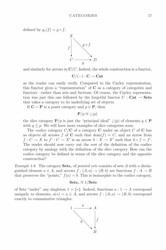
The coslice category C/C of a category C under an object C of C hasas objects all arrows f of C such that dom(f) = C, and an arrow fromf : C → X to f ′ : C → X ′ is an arrow h : X → X ′ such that h ◦ f = f ′.The reader should now carry out the rest of the definition of the coslicecategory by analogy with the definition of the slice category. How can thecoslice category be defined in terms of the slice category and the oppositeconstruction?
Example 1.8. The category Sets∗ of pointed sets consists of sets A with a distin-guished element a ∈ A, and arrows f : (A, a) → (B, b) are functions f : A → Bthat preserves the “points,” f(a) = b. This is isomorphic to the coslice category,
Sets∗ ∼= 1/Sets
of Sets “under” any singleton 1 = {∗}. Indeed, functions a : 1 → A corresponduniquely to elements, a(∗) = a ∈ A, and arrows f : (A, a) → (B, b) correspondexactly to commutative triangles:
1a � A
B
f
�b
�

18 CATEGORY THEORY
1.7 Free categories
Free monoid. Start with an “alphabet” A of “letters” a, b, c, . . . , that is, a set,
A = {a, b, c, . . .}.
A word over A is a finite sequence of letters:
thisword, categoriesarefun, asddjbnzzfj, . . .
We write “-” for the empty word. The “Kleene closure” of A is defined to bethe set
A∗ = {words over A}.
Define a binary operation “∗” on A∗ by w ∗ w′ = ww′ for words w,w′ ∈ A∗.Thus, “∗” is just concatenation. The operation “∗” is thus associative, and theempty word “-” is a unit. Thus, A∗ is a monoid—called the free monoid onthe set A. The elements a ∈ A can be regarded as words of length one, so wehave a function
i : A → A∗
defined by i(a) = a, and called the “insertion of generators.” The elements of A“generate” the free monoid, in the sense that every w ∈ A∗ is a ∗-product of a’s,that is, w = a1 ∗ a2 ∗ · · · ∗ an for some a1, a2, ..., an in A.
Now what does “free” mean here? Any guesses? One sometimes seesdefinitions in “baby algebra” books along the following lines:
A monoid M is freely generated by a subset A of M , if the following conditionshold:
1. Every element m ∈ M can be written as a product of elements of A:
m = a1 ·M . . . ·M an , ai ∈ A.
2. No “nontrivial” relations hold in M , that is, if a1 . . . aj = a′1 . . . a′
k, thenthis is required by the axioms for monoids.
The first condition is sometimes called “no junk,” while the second condition issometimes called “no noise.” Thus, the free monoid on A is a monoid containingA and having no junk and no noise. What do you think of this definition of afree monoid?
I would object to the reference in the second condition to “provability,” orsomething. This must be made more precise for this to succeed as a definition. Incategory theory, we give a precise definition of “free”—capturing what is meantin the above—which avoids such vagueness.
First, every monoid N has an underlying set |N |, and every monoid homo-morphism f : N → M has an underlying function |f | : |N | → |M |. It is easy tosee that this is a functor, called the “forgetful functor.” The free monoid M(A)

CATEGORIES 19
on a set A is by definition “the” monoid with the following so called universalmapping property or UMP!
Universal Mapping Property of M(A)There is a function i : A → |M(A)|, and given any monoid N and any functionf : A → |N |, there is a unique monoid homomorphism f : M(A) → N such that|f | ◦ i = f , all as indicated in the following diagram:
in Mon:
M(A) ...............f
� N
in Sets:
|M(A)| |f |� |N |
A
i
�
f
�
Proposition 1.9. A∗ has the UMP of the free monoid on A.
Proof. Given f : A → |N |, define f : A∗ → N by
f(−) = uN , the unit of N
f(a1 . . . ai) = f(a1) ·N . . . ·N f(ai).
Then, f is clearly a homomorphism with
f(a) = f(a) for all a ∈ A.
If g : A∗→N also satisfies g(a)= f(a) for all a ∈ A, then for all a1 . . . ai ∈ A∗:
g(a1 . . . ai) = g(a1 ∗ . . . ∗ ai)
= g(a1) ·N . . . ·N g(ai)
= f(a1) ·N . . . ·N f(ai)
= f(a1) ·N . . . ·N f(ai)
= f(a1 ∗ . . . ∗ ai)
= f(a1 . . . ai).
So, g = f , as required.
Think about why the above UMP captures precisely what is meant by “no junk”and “no noise.” Specifically, the existence part of the UMP captures the vaguenotion of “no noise” (because any equation that holds between algebraic combi-nations of the generators must also hold anywhere they can be mapped to, and

20 CATEGORY THEORY
thus everywhere), while the uniqueness part makes precise the “no junk” idea(because any extra elements not combined from the generators would be free tobe mapped to different values).
Using the UMP, it is easy to show that the free monoid M(A) is determineduniquely up to isomorphism, in the following sense.
Proposition 1.10. Given monoids M and N with functions i : A→|M | andj : A → |N |, each with the UMP of the free monoid on A, there is a (unique)monoid isomorphism h : M ∼= N such that |h|i = j and |h−1|j = i.
Proof. From j and the UMP of M , we have j : M → N with |j|i = j and fromi and the UMP of N , we have i : N → M with |i|j = i. Composing gives ahomomorphism i ◦ j : M → M such that |i ◦ j|i = i. Since 1M : M → M alsohas this property, by the uniqueness part of the UMP of M , we have i ◦ j = 1M .Exchanging the roles of M and N shows j ◦ i = 1N :
in Mon:
M ...................j
� N ...................i
� M
in Sets:
|M | |j| � |N | |i| � |M |
A
j
�
i
�
i
�
For example, the free monoid on any set with a single element is easily seen tobe isomorphic to the monoid of natural numbers N under addition (the “gene-rator” is the number 1). Thus, as a monoid, N is uniquely determined up toisomorphism by the UMP of free monoids.
Free category. Now, we want to do the same thing for categories in general(not just monoids). Instead of underlying sets, categories have underlying graphs,so let us review these first.
A directed graph consists of vertices and edges, each of which is directed, thatis, each edge has a “source” and a “target” vertex.
Az � B
C
x
�
D
y
�
u�

CATEGORIES 21
We draw graphs just like categories, but there is no composition of edges, andthere are no identities.
A graph thus consists of two sets, E (edges) and V (vertices), and two func-tions, s : E → V (source) and t : E → V (target). Thus, in Sets, a graph is justa configuration of objects and arrows of the form
Es �
t� V
Now, every graph G “generates” a category C(G), the free category on G. Itis defined by taking the vertices of G as objects, and the paths in G as arrows,where a path is a finite sequence of edges e1, . . . , en such that t(ei) = s(ei+1),for all i = 1 . . . n. We’ write the arrows of C(G) in the form enen−1 . . . e1.
v0e1 � v1
e2 � v2e3 � . . .
en � vn
Put
dom(en . . . e1) = s(e1)
cod(en . . . e1) = t(en)
and define composition by concatenation:
en . . . e1 ◦ e′m . . . e′1 = en . . . e1e′m . . . e′1.
For each vertex v, we have an “empty path” denoted by 1v, which is to be theidentity arrow at v.
Note that if G has only one vertex, then C(G) is just the free monoid on theset of edges of G. Also note that if G has only vertices (no edges), then C(G) isthe discrete category on the set of vertices of G.
Later on, we will have a general definition of “free.” For now, let us see thatC(G) also has a UMP. First, define a “forgetful functor”
U : Cat → Graphs
in the obvious way: the underlying graph of a category C has as edges the arrowsof C, and as vertices the objects, with s = dom and t = cod. The action of U onfunctors is equally clear, or at least it will be, once we have defined the arrowsin Graphs.
A homomorphism of graphs is of course a “functor without the conditions onidentities and composition,” that is, a mapping of edges to edges and verticesto vertices that preserves sources and targets. We describe this from a slightlydifferent point of view, which will be useful later on.
First, observe that we can describe a category C with a diagram like this:
C2◦ � C1
cod �� i
dom� C0

22 CATEGORY THEORY
where C0 is the collection of objects of C, C1 the arrows, i is the identity arrowoperation, and C2 is the collection {(f, g) ∈ C1 × C1 : cod(f) = dom(g)}.
Then a functor F : C → D from C to another category D is a pair offunctions
F0 : C0 → D0
F1 : C1 → D1
such that each similarly labeled square in the following diagram commutes:
C2◦ � C1
cod �� i
dom� C0
D2
F2
�
◦� D1
F1
� cod �� i
dom� D0
F0
�
where F2(f, g) = (F1(f), F1(g)).Now let us describe a homomorphism of graphs,
h : G → H.
We need a pair of functions h0 : G0 → H0, h1 : G1 → H1 making the two squares(once with t’s, once with s’s) in the following diagram commute:
G1
t �
s� G0
H1
h1
� t �
s� H0
h0
�
In these terms, we can easily describe the forgetful functor,
U : Cat → Graphs
as sending the category
C2◦ � C1
cod �� i
dom� C0
to the underlying graph
C1
cod �
dom� C0.

CATEGORIES 23
And similarly for functors, the effect of U is described by simply erasing someparts of the diagrams (which is easier to demonstrate with chalk!). Let us againwrite |C| = U(C), etc., for the underlying graph of a category C, in analogy tothe case of monoids above.
The free category on a graph now has the following UMP.
Universal Mapping Property of C(G)There is a graph homomorphism i : G → |C(G)|, and given any category D andany graph homomorphism h : G → |D|, there is a unique functor h : C(G) → Dwith |h| ◦ i = h.
in Cat:
C(G) ................h
� D
in Graph:
|C(G)| |h|� |D|
G
i
�
h
�
The free category on a graph with just one vertex is just a free monoid onthe set of edges. The free category on a graph with two vertices and one edgebetween them is the finite category 2. The free category on a graph of the form
Ae ��f
B
has (in addition to the identity arrows) the infinitely many arrows:
e, f, ef, fe, efe, fef, efef, ...
1.8 Foundations: large, small, and locally small
Let us begin by distinguishing between the following things:
(i) categorical foundations for mathematics,(ii) mathematical foundations for category theory.
As for the first point, one sometimes hears it said that category theory can beused to provide “foundations for mathematics,” as an alternative to set theory.That is in fact the case, but it is not what we are doing here. In set theory,one often begins with existential axioms such as “there is an infinite set” and

24 CATEGORY THEORY
derives further sets by axioms like “every set has a powerset,” thus building up auniverse of mathematical objects (namely sets), which in principle suffice for “allof mathematics.” Our axiom that every arrow has a domain and a codomain isnot to be understood in the same way as set theory’s axiom that every set has apowerset! The difference is that in set theory—at least as usually conceived—theaxioms are to be regarded as referring to (or determining) a single universe of sets.In category theory, by contrast, the axioms are a definition of something, namelyof categories. This is just like in group theory or topology, where the axioms serveto define the objects under investigation. These, in turn, are assumed to exist insome “background” or “foundational” system, like set theory (or type theory).That theory of sets could itself, in turn, be determined using category theory, orin some other way.
This brings us to the second point: we assume that our categories are compri-sed of sets and functions, in one way or another, like most mathematical objects,and taking into account the remarks just made about the possibility of cate-gorical (or other) foundations. But in category theory, we sometimes run intodifficulties with set theory as usually practiced. Mostly these are questions ofsize; some categories are “too big” to be handled comfortably in conventionalset theory. We already encountered this issue when we considered the Cayleyrepresentation in Section 1.5. There we had to require that the category underconsideration had (no more than) a set of arrows. We would certainly not want toimpose this restriction in general, however (as one usually does for, say, groups);for then even the “category” Sets would fail to be a proper category, as wouldmany other categories that we definitely want to study.
There are various formal devices for addressing these issues, and they arediscussed in the book by Mac Lane. For our immediate purposes, the followingdistinction will be useful.
Definition 1.11. A category C is called small if both the collection C0 ofobjects of C and the collection C1 of arrows of C are sets. Otherwise, C iscalled large.
For example, all finite categories are clearly small, as is the category Setsfin offinite sets and functions. (Actually, one should stipulate that the sets are onlybuilt from other finite sets, all the way down, i.e., that they are “hereditarilyfinite”.) On the other hand, the category Pos of posets, the category Groups ofgroups, and the category Sets of sets are all large. We let Cat be the categoryof all small categories, which itself is a large category. In particular, then, Catis not an object of itself, which may come as a relief to some readers.
This does not really solve all of our difficulties. Even for large categories likeGroups and Sets we will want to also consider constructions like the categoryof all functors from one to the other (we define this “functor category” later).But if these are not small, conventional set theory does not provide the meansto do this directly (these categories would be “too large”). Therefore, one needsa more elaborate theory of “classes” to handle such constructions. We will not

CATEGORIES 25
worry about this when it is just a matter of technical foundations (Mac Lane I.6addresses this issue). However, one very useful notion in this connection is thefollowing.
Definition 1.12. A category C is called locally small if for all objects X, Yin C, the collection HomC(X,Y ) = {f ∈ C1 | f : X → Y } is a set (called ahom-set).
Many of the large categories we want to consider are, in fact, locally small. Setsis locally small since HomSets(X,Y ) = Y X , the set of all functions from X to Y .Similarly, Pos, Top, and Group are all locally small (is Cat?), and, of course,any small category is locally small.
Warning 1.13. Do not confuse the notions concrete and small. To say that acategory is concrete is to say that the objects of the category are (structured)sets, and the arrows of the category are (certain) functions. To say that a categoryis small is to say that the collection of all objects of the category is a set, as isthe collection of all arrows. The real numbers R, regarded as a poset category, issmall but not concrete. The category Pos of all posets is concrete but not small.
1.9 Exercises
1. The objects of Rel are sets, and an arrow A → B is a relation from A to B,that is, a subset R ⊆ A×B. The equality relation {〈a, a〉 ∈ A×A| a ∈ A}is the identity arrow on a set A. Composition in Rel is to be given by
S ◦R = {〈a, c〉 ∈ A× C | ∃b (〈a, b〉 ∈ R & 〈b, c〉 ∈ S)}
for R ⊆ A×B and S ⊆ B × C.
(a) Show that Rel is a category.(b) Show also that there is a functor G : Sets → Rel taking objects to
themselves and each function f : A → B to its graph,
G(f) = {〈a, f(a)〉 ∈ A×B | a ∈ A}.
(c) Finally, show that there is a functor C : Relop → Rel taking eachrelation R ⊆ A×B to its converse Rc ⊆ B ×A, where,
〈a, b〉 ∈ Rc ⇔ 〈b, a〉 ∈ R.
2. Consider the following isomorphisms of categories and determine whichhold.
(a) Rel ∼= Relop
(b) Sets ∼= Setsop

26 CATEGORY THEORY
(c) For a fixed set X with powerset P (X), as poset categories P (X) ∼=P (X)op (the arrows in P (X) are subset inclusions A ⊆ B for allA,B ⊆ X).
3. (a) Show that in Sets, the isomorphisms are exactly the bijections.(b) Show that in Monoids, the isomorphisms are exactly the bijective
homomorphisms.(c) Show that in Posets, the isomorphisms are not the same as the
bijective homomorphisms.4. Let X be a topological space and preorder the points by specialization:
x ≤ y iff y is contained in every open set that contains x. Show that thisis a preorder, and that it is a poset if X is T0 (for any two distinct points,there is some open set containing one but not the other). Show that theordering is trivial if X is T1 (for any two distinct points, each is containedin an open set not containing the other).
5. For any category C, define a functor U : C/C → C from the slice categoryover an object C that “forgets about C.” Find a functor F : C/C → C→
to the arrow category such that dom ◦ F = U .6. Construct the “coslice category” C/C of a category C under an object C
from the slice category C/C and the “dual category” operation −op.7. Let 2 = {a, b} be any set with exactly 2 elements a and b. Define a functor
F : Sets/2 → Sets× Sets with F (f : X → 2) = (f−1(a), f−1(b)). Is thisan isomorphism of categories? What about the analogous situation with aone-element set 1 = {a} instead of 2?
8. Any category C determines a preorder P (C) by defining a binary rela-tion ≤ on the objects by
A ≤ B if and only if there is an arrow A → B
Show that P determines a functor from categories to preorders, by defi-ning its effect on functors between categories and checking the requiredconditions. Show that P is a (one-sided) inverse to the evident inclusionfunctor of preorders into categories.
9. Describe the free categories on the following graphs by determining theirobjects, arrows, and composition operations.
(a)
ae � b
(b)
ae ��f
b

CATEGORIES 27
(c)
ae � b
c
f
�
g�
(d)
ae ��h
b d
c
f
�
g
�
10. How many free categories on graphs are there which have exactly sixarrows? Draw the graphs that generate these categories.
11. Show that the free monoid functor
M : Sets → Mon
exists, in two different ways:
(a) Assume the particular choice M(X) = X∗ and define its effect
M(f) : M(A) → M(B)
on a function f : A → B to be
M(f)(a1 . . . ak) = f(a1) . . . f(ak), a1, . . . ak ∈ A.
(b) Assume only the UMP of the free monoid and use it to determine Mon functions, showing the result to be a functor.
Reflect on how these two approaches are related.12. Verify the UMP for free categories on graphs, defined as above with arrows
being sequences of edges. Specifically, let C(G) be the free category on thegraph G, so defined, and i : G → U(C(G)) the graph homomorphismtaking vertices and edges to themselves, regarded as objects and arrows inC(G). Show that for any category D and graph homomorphism f : G →U(D), there is a unique functor
h : C(G) → D
with
U(h) ◦ i = h,

28 CATEGORY THEORY
where U : Cat → Graph is the underlying graph functor.13. Use the Cayley representation to show that every small category is iso-
morphic to a “concrete” one, that is, one in which the objects are sets andthe arrows are functions between them.
14. The notion of a category can also be defined with just one sort (arrows)rather than two (arrows and objects); the domains and codomains aretaken to be certain arrows that act as units under composition, which ispartially defined. Read about this definition in section I.1 of Mac Lane’sCategories for the Working Mathematician, and do the exercise mentionedthere, showing that it is equivalent to the usual definition.

2
ABSTRACT STRUCTURES
We begin with some remarks about category-theoretical definitions. These arecharacterizations of properties of objects and arrows in a category solely in termsof other objects and arrows, that is, just in the language of category theory.Such definitions may be said to be abstract, structural, operational, relational,or perhaps external (as opposed to internal). The idea is that objects and arrowsare determined by the role they play in the category via their relations to otherobjects and arrows, that is, by their position in a structure and not by whatthey “are” or “are made of” in some absolute sense. The free monoid or categoryconstruction of the foregoing chapter was an example of one such definition, andwe see many more examples of this kind later; for now, we start with some verysimple ones. Let us call them abstract characterizations. We see that one of thebasic ways of giving such an abstract characterization is via a Universal MappingProperty (UMP).
2.1 Epis and monos
Recall that in Sets, a function f : A → B is called
injective if f(a) = f(a′) implies a = a′ for all a, a′ ∈ A,surjective if for all b ∈ B there is some a ∈ A with f(a) = b.
We have the following abstract characterizations of these properties.
Definition 2.1. In any category C, an arrow
f : A → B
is called a
monomorphism, if given any g, h : C → A, fg = fh implies g = h,
Cg �
h� A
f � B
epimorphism, if given any i, j : B → D, if = jf implies i = j,
Af � B
i �
j� D.

30 CATEGORY THEORY
We often write f : A � B if f is a monomorphism and f : A � B if f is anepimorphism.
Proposition 2.2. A function f : A → B between sets is monic just in case itis injective.
Proof. Suppose f : A � B. Let a, a′ ∈ A such that a �= a′, and let {x} be anygiven one-element set. Consider the functions
a, a′ : {x} → A
where
a(x) = a, a′(x) = a′.
Since a �= a′, it follows, since f is a monomorphism, that fa �= fa′. Thus,f(a) = (fa)(x) �= (fa′)(x) = f(a′). Whence f is injective.
Conversely, if f is injective and g, h : C → A are functions such that g �= h,then for some c ∈ C, g(c) �= h(c). Since f is injective, it follows that f(g(c)) �=f(h(c)), whence fg �= fh.
Example 2.3. In many categories of “structured sets” like monoids, the monosare exactly the “injective homomorphisms.” More precisely, a homomorphismh : M → N of monoids is monic just if the underlying function |h| : |M | →|N | is monic, that is, injective by the foregoing. To prove this, suppose h ismonic and take two different “elements” x, y : 1 → |M |, where 1 = {∗} isany one-element set. By the UMP of the free monoid M(1) there are distinctcorresponding homomorphisms x, y : M(1) → M , with distinct composites h ◦x, h◦ y : M(1) → M → N , since h is monic. Thus, the corresponding “elements”hx, hy : 1 → N of N are also distinct, again by the UMP of M(1).
M(1)x �
y� M
h � N
1x �
y� |M | |h| � |N |
Conversely, if |h| : |M | → |N | is monic and f, g : X → M are any distincthomomorphisms, then |f |, |g| : |X| → |M | are distinct functions, and so |h| ◦|f |, |h| ◦ |g| : |X| → |M | → |N | are distinct, since |h| is monic. Since therefore|h ◦ f | = |h| ◦ |f | �= |h| ◦ |g| = |h ◦ g|, we also must have h ◦ f �= h ◦ g.
A completely analogous situation holds, for example, for groups, rings, vectorspaces, and posets. We shall see that this fact follows from the presence, in eachof these categories, of certain objects like the free monoid M(1).
Example 2.4. In a poset P, every arrow p ≤ q is both monic and epic. Why?

ABSTRACT STRUCTURES 31
Now, dually to the foregoing, the epis in Sets are exactly the surjectivefunctions (exercise!); by contrast, however, in many other familiar categories theyare not just the surjective homomorphisms, as the following example shows.
Example 2.5. In the category Mon of monoids and monoid homomorphisms,there is a monic homomorphism
N � Z
where N is the additive monoid (N, +, 0) of natural numbers and Z is the additivemonoid (Z,+, 0) of integers. We show that this map, given by the inclusionN ⊂ Z of sets, is also epic in Mon by showing that the following holds:
Given any monoid homomorphisms f, g : (Z,+, 0) → (M, ∗, u), if therestrictions to N are equal, f |N= g |N , then f = g.
Note first that
f(−n) = f((−1)1 + (−1)2 + · · ·+ (−1)n)
= f(−1)1 ∗ f(−1)2 ∗ · · · ∗ f(−1)n
and similarly for g. It, therefore, suffices to show that f(−1) = g(−1). But
f(−1) = f(−1) ∗ u
= f(−1) ∗ g(0)
= f(−1) ∗ g(1− 1)
= f(−1) ∗ g(1) ∗ g(−1)
= f(−1) ∗ f(1) ∗ g(−1)
= f(−1 + 1) ∗ g(−1)
= f(0) ∗ g(−1)
= u ∗ g(−1)
= g(−1).
Note that, from an algebraic point of view, a morphism e is epic if and onlyif e cancels on the right: xe = ye implies x = y. Dually, m is monic if and onlyif m cancels on the left: mx = my implies x = y.
Proposition 2.6. Every iso is both monic and epic.
Proof. Consider the following diagram:
Ax �
y� B
m � C
B
e
� ��
1�
D

32 CATEGORY THEORY
If m is an isomorphism with inverse e, then mx = my implies x = emx =emy = y. Thus, m is monic. Similarly, e cancels on the right and thus is epic.
In Sets, the converse of the foregoing also holds: every mono-epi is iso. But thisis not in general true, as shown by the example in monoids above.
2.1.1 Sections and retractions
We have just noted that any iso is both monic and epic. More generally, if anarrow
f : A → B
has a left inverse
g : B → A, gf = 1A
then f must be monic and g epic, by the same argument.
Definition 2.7. A split mono (epi) is an arrow with a left (right) inverse. Givenarrows e : X → A and s : A → X such that es = 1A, the arrow s is called asection or splitting of e, and the arrow e is called a retraction of s. The objectA is called a retract of X.
Since functors preserve identities, they also preserve split epis and splitmonos. Compare example 2.5 above in Mon where the forgetful functor
Mon → Set
did not preserve the epi N → Z.
Example 2.8. In Sets, every mono splits except those of the form
∅ � A.
The condition that every epi splits is the categorical version of the axiom ofchoice. Indeed, consider an epi
e : E � X.
We have the family of nonempty sets:
Ex = e−1{x}, x ∈ X.
A choice function for this family (Ex)x∈X is exactly a splitting of e, that is, afunction s : X → E such that es = 1X , since this means that s(x) ∈ Ex for allx ∈ X.
Conversely, given a family of nonempty sets,
(Ex)x∈X
take E = {(x, y) | x ∈ X, y ∈ Ex} and define the epi e : E � X by (x, y) �→ x.A splitting s of e then determines a choice function for the family.

ABSTRACT STRUCTURES 33
The idea that a “family of objects” (Ex)x∈X can be represented by a singlearrow e : E → X by using the “fibers” e−1(x) has much wider application thanthis, and is considered further in Section 7.10.
A notion related to the existence of “choice functions” is that of being “pro-jective”: an object P is said to be projective if for any epi e : E � X and arrowf : P → X there is some (not necessarily unique) arrow f : P → E such thate ◦ f = f , as indicated in the following diagram:
E
Pf
�
f.....
..........
..........
.......�
X
e
��
One says that f lifts across e. Any epi into a projective object clearly splits.Projective objects may be thought of as having a more “free” structure, thuspermitting “more arrows.”
The axiom of choice implies that all sets are projective, and it follows thatfree objects in many (but not all!) categories of algebras then are also projective.The reader should show that, in any category, any retract of a projective objectis also projective.
2.2 Initial and terminal objects
We now consider abstract characterizations of the empty set and the one-element sets in the category Sets and structurally similar objects in generalcategories.
Definition 2.9. In any category C, an object
0 is initial if for any object C there is a unique morphism
0 → C,
1 is terminal if for any object C there is a unique morphism
C → 1.
As in the case of monos and epis, note that there is a kind of “duality” inthese definitions. Precisely, a terminal object in C is exactly an initial object inCop. We consider this duality systematically in Chapter 3.
First, observe that since the notions of initial and terminal object are simpleUMPs, such objects are uniquely determined up to isomorphism, just like thefree monoids were.
Proposition 2.10. Initial (terminal) objects are unique up to isomorphism.

34 CATEGORY THEORY
Proof. In fact, if C and C ′ are both initial (terminal) in the same category, thenthere is a unique isomorphism C → C ′. Indeed, suppose that 0 and 0′ are bothinitial objects in some category C; the following diagram then makes it clearthat 0 and 0′ are uniquely isomorphic:
0u � 0′
0
v
�
u�
10�
0′
10′
�
For terminal objects, apply the foregoing to Cop.
Example 2.11.
1. In Sets, the empty set is initial and any singleton set {x} is terminal.Observe that Sets has just one initial object but many terminal objects(answering the question of whether Sets ∼= Setsop).
2. In Cat, the category 0 (no objects and no arrows) is initial and the category1 (one object and its identity arrow) is terminal.
3. In Groups, the one-element group is both initial and terminal (similarlyfor the category of vector spaces and linear transformations, as well as thecategory of monoids and monoid homomorphisms). But in Rings (commu-tative with unit), the ring Z of integers is initial (the one-element ring with0 = 1 is terminal).
4. A Boolean algebra is a poset B equipped with distinguished elements 0, 1,binary operations a∨ b of “join” and a∧ b of “meet,” and a unary operation¬b of “complementation.” These are required to satisfy the conditions
0 ≤ a
a ≤ 1
a ≤ c and b ≤ c iff a ∨ b ≤ c
c ≤ a and c ≤ b iff c ≤ a ∧ b
a ≤ ¬b iff a ∧ b = 0
¬¬a = a.
There is also an equivalent, fully equational characterization not invol-ving the ordering. A typical example of a Boolean algebra is the powersetP(X) of all subsets A ⊆ X of a set X, ordered by inclusion A ⊆ B, andwith the Boolean operations being the empty set 0 = ∅, the whole set1 = X, union and intersection of subsets as join and meet, and the rela-tive complement X − A as ¬A. A familiar special case is the two-element

ABSTRACT STRUCTURES 35
Boolean algebra 2 = {0, 1} (which may be taken to be the powerset P(1)),sometimes also regarded as “truth values” with the logical operations ofdisjunction, conjunction, and negation as the Boolean operations. It is aninitial object in the category BA of Boolean algebras. BA has as arrowsthe Boolean homomorphisms, that is, functors h : B → B′ that preservethe additional structure, in the sense that h(0) = 0, h(a ∨ b) = h(a) ∨ h(b),etc. The one-element Boolean algebra (i.e., P(0)) is terminal.
5. In a poset, an object is plainly initial iff it is the least element, and terminaliff it is the greatest element. Thus, for instance, any Boolean algebra hasboth. Obviously, a category need not have either an initial object or aterminal object; for example, the poset (Z,≤) has neither.
6. For any category C and any object X ∈ C, the identity arrow 1X : X → Xis a terminal object in the slice category C/X and an initial object in thecoslice category X/C.
2.3 Generalized elements
Let us consider arrows into and out of initial and terminal objects. Clearly onlycertain of these will be of interest, but those are often especially significant.
A set A has an arrow into the initial object A → 0 just if it is itself initial,and the same is true for posets. In monoids and groups, by contrast, every objecthas a unique arrow to the initial object, since it is also terminal.
In the category BA of Boolean algebras, however, the situation is quite diffe-rent. The maps p : B → 2 into the initial Boolean algebra 2 correspond uniquelyto the so-called ultrafilters U in B. A filter in a Boolean algebra B is a nonemptysubset F ⊆ B that is closed upward and under meets:
a ∈ F and a ≤ b implies b ∈ F
a ∈ F and b ∈ F implies a ∧ b ∈ F
A filter F is maximal if the only strictly larger filter F ⊂ F ′ is the “improper”filter, namely all of B. An ultrafilter is a maximal filter. It is not hard to see thata filter F is an ultrafilter just if for every element b ∈ B, either b ∈ F or ¬b ∈ F ,and not both (exercise!). Now if p : B → 2, let Up = p−1(1) to get an ultrafilterUp ⊂ B. And given an ultrafilter U ⊂ B, define pU (b) = 1 iff b ∈ U to get aBoolean homomorphism pU : B → 2. This is easy to check, as is the fact thatthese operations are mutually inverse. Boolean homomorphisms B → 2 are alsoused in forming the “truth tables” one meets in logic. Indeed, a row of a truthtable corresponds to such a homomorphism on a Boolean algebra of formulas.
Ring homomorphisms A → Z into the initial ring Z play an analogous andequally important role in algebraic geometry. They correspond to so-called primeideals, which are the ring-theoretic generalizations of ultrafilters.

36 CATEGORY THEORY
Now let us consider some arrows from terminal objects. For any set X, forinstance, we have an isomorphism
X ∼= HomSets(1, X)
between elements x ∈ X and arrows x : 1 → X, determined by x(∗) = x, froma terminal object 1 = {∗}. We have already used this correspondence severaltimes. A similar situation holds in posets (and in topological spaces), where thearrows 1 → P correspond to elements of the underlying set of a poset (or space)P . In any category with a terminal object 1, such arrows 1 → A are often calledglobal elements, or points, or constants of A. In sets, posets, and spaces, thegeneral arrows A → B are determined by what they do to the points of A, inthe sense that two arrows f, g : A → B are equal if for every point a : 1 → A thecomposites are equal, fa = ga.
But be careful; this is not always the case! How many points are there of anobject M in the category of monoids? That is, how many arrows of the form1 → M for a given monoid M? Just one! And how many points does a Booleanalgebra have?
Because, in general, an object is not determined by its points, it is convenientto introduce the device of generalized elements. These are arbitrary arrows,
x : X → A
(with arbitrary domain X), which can be regarded as generalized or variableelements of A. Computer scientists and logicians sometimes think of arrows1 → A as constants or closed terms and general arrows X → A as arbitraryterms. Summarizing:
Example 2.12.
1. Consider arrows f, g : P → Q in Pos. Then f = g iff for all x : 1 → P , wehave fx = gx. In this sense, posets “have enough points” to separate thearrows.
2. By contrast, in Mon, for homomorphisms h, j : M → N , we always havehx = jx, for all x : 1 → M , since there is just one such point x. Thus,monoids do not “have enough points.”
3. But in any category C, and for any arrows f, g : C → D, we always havef = g iff for all x : X → C, it holds that fx = gx (why?). Thus, all objectshave enough generalized elements.
4. In fact, it often happens that it is enough to consider generalized elementsof just a certain form T → A, that is, for certain “test” objects T . We shallconsider this presently.
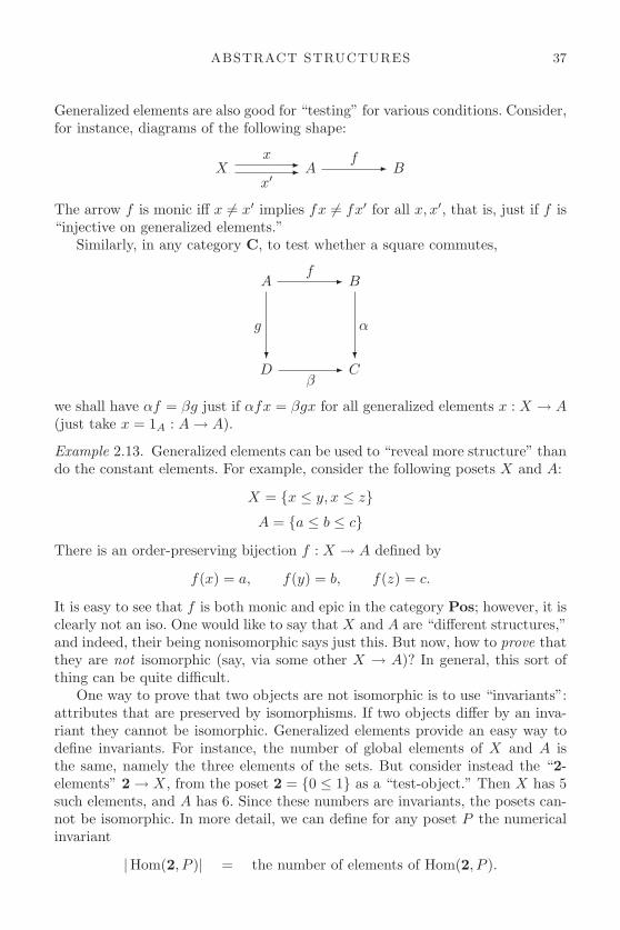
ABSTRACT STRUCTURES 37
Generalized elements are also good for “testing” for various conditions. Consider,for instance, diagrams of the following shape:
Xx �
x′� A
f � B
The arrow f is monic iff x �= x′ implies fx �= fx′ for all x, x′, that is, just if f is“injective on generalized elements.”
Similarly, in any category C, to test whether a square commutes,
Af � B
D
g
�
β� C
α
�
we shall have αf = βg just if αfx = βgx for all generalized elements x : X → A(just take x = 1A : A → A).
Example 2.13. Generalized elements can be used to “reveal more structure” thando the constant elements. For example, consider the following posets X and A:
X = {x ≤ y, x ≤ z}A = {a ≤ b ≤ c}
There is an order-preserving bijection f : X → A defined by
f(x) = a, f(y) = b, f(z) = c.
It is easy to see that f is both monic and epic in the category Pos; however, it isclearly not an iso. One would like to say that X and A are “different structures,”and indeed, their being nonisomorphic says just this. But now, how to prove thatthey are not isomorphic (say, via some other X → A)? In general, this sort ofthing can be quite difficult.
One way to prove that two objects are not isomorphic is to use “invariants”:attributes that are preserved by isomorphisms. If two objects differ by an inva-riant they cannot be isomorphic. Generalized elements provide an easy way todefine invariants. For instance, the number of global elements of X and A isthe same, namely the three elements of the sets. But consider instead the “2-elements” 2 → X, from the poset 2 = {0 ≤ 1} as a “test-object.” Then X has 5such elements, and A has 6. Since these numbers are invariants, the posets can-not be isomorphic. In more detail, we can define for any poset P the numericalinvariant
|Hom(2, P )| = the number of elements of Hom(2, P ).

38 CATEGORY THEORY
Then if P ∼= Q, it is easy to see that |Hom(2, P )| = |Hom(2, Q)|, since anyisomorphism
Pi ��j
Q
also gives an iso
Hom(2, P )i∗ ��j∗
Hom(2, Q)
defined by composition:
i∗(f) = if
j∗(g) = jg
for all f : 2 → P and g : 2 → Q. Indeed, this is a special case of the very generalfact that Hom(X,−) is always a functor, and functors always preserve isos.
Example 2.14. As in the foregoing example, it is often the case that generalizedelements t : T → A “based at” certain objects T are especially “revealing.” Wecan think of such elements geometrically as “figures of shape T in A,” just as anarrow 2 → P in posets is a figure of shape p ≤ p′ in P . For instance, as we havealready seen, in the category of monoids, the arrows from the terminal monoid areentirely uninformative, but those from the free monoid on one generator M(1)suffice to distinguish homomorphisms, in the sense that two homomorphismsf, g : M → M ′ are equal if their composites with all such arrows are equal.Since we know that M(1) = N, the monoid of natural numbers, we can think ofgeneralized elements M(1) → M based at M(1) as “figures of shape N” in M .In fact, by the UMP of M(1), the underlying set |M | is therefore (isomorphicto) the collection HomMon(N,M) of all such figures, since
|M | ∼= HomSets(1, |M |) ∼= HomMon(N,M).
In this sense, a map from a monoid is determined by its effect on all of the figuresof shape N in the monoid.
2.4 Products
Next, we are going to see the categorical definition of a product of two objects in acategory. This was first given by Mac Lane in 1950, and it is probably the earliestexample of category theory being used to define a fundamental mathematicalnotion.
By “define” here I mean an abstract characterization, in the sense alreadyused, in terms of objects and arrows in a category. And as before, we do this bygiving a UMP, which determines the structure at issue up to isomorphism, as

ABSTRACT STRUCTURES 39
usual in category theory. Later in this chapter, we have several other examplesof such characterizations.
Let us begin by considering products of sets. Given sets A and B, the cartesianproduct of A and B is the set of ordered pairs
A×B = {(a, b) | a ∈ A, b ∈ B}.Observe that there are two “coordinate projections”
A � π1A×B
π2 � B
with
π1(a, b) = a, π2(a, b) = b.
And indeed, given any element c ∈ A×B, we have
c = (π1c, π2c).
The situation is captured concisely in the following diagram:
1
A �π1
a
�
A×B
(a,b)
�
.................
π2
� B
b
�
Replacing elements by generalized elements, we get the following definition.
Definition 2.15. In any category C, a product diagram for the objects A andB consists of an object P and arrows
A � p1P
p2 � B
satisfying the following UMP:Given any diagram of the form
A � x1X
x2 � B
there exists a unique u : X → P , making the diagram
X
A �p1
x1
�
P
u
�
.................
p2
� B
x2
�
commute, that is, such that x1 = p1u and x2 = p2u.

40 CATEGORY THEORY
Remark 2.16. As in other UMPs, there are two parts:
Existence: There is some u : X → U such that x1 = p1u and x2 = p2u.Uniqueness: Given any v : X → U , if p1v = x1 and p2v = x2, then v = u.
Proposition 2.17. Products are unique up to isomorphism.
Proof. Suppose
A � p1P
p2 � B
and
A � q1Q
q2 � B
are products of A and B. Then, since Q is a product, there is a unique i : P → Qsuch that q1 ◦ i = p1 and q2 ◦ i = p2. Similarly, since P is a product, there is aunique j : Q → P such that p1 ◦ j = q1 and p2 ◦ j = q2.
P
A �q1
p1
�
Q
i
�
.................
q2
� B
p2
�
P
j
�
................p2
�
p1
�
Composing, p1 ◦ j ◦ i = p1 and p2 ◦ j ◦ i = p2. Since also p1 ◦ 1P = p1 andp2 ◦ 1P = p2, it follows from the uniqueness condition that j ◦ i = 1P . Similarly,we can show i ◦ j = 1Q. Thus, i : P → Q is an isomorphism.
If A and B have a product, we write
A � p1A×B
p2 � B
for one such product. Then given X,x1, x2 as in the definition, we write
〈x1, x2〉 for u : X → A×B.
Note, however, that a pair of objects may have many different products in acategory. For example, given a product A×B, p1, p2, and any iso h : A×B → Q,the diagram Q, p1 ◦ h, p2 ◦ h is also a product of A and B.
Now an arrow into a product
f : X → A×B
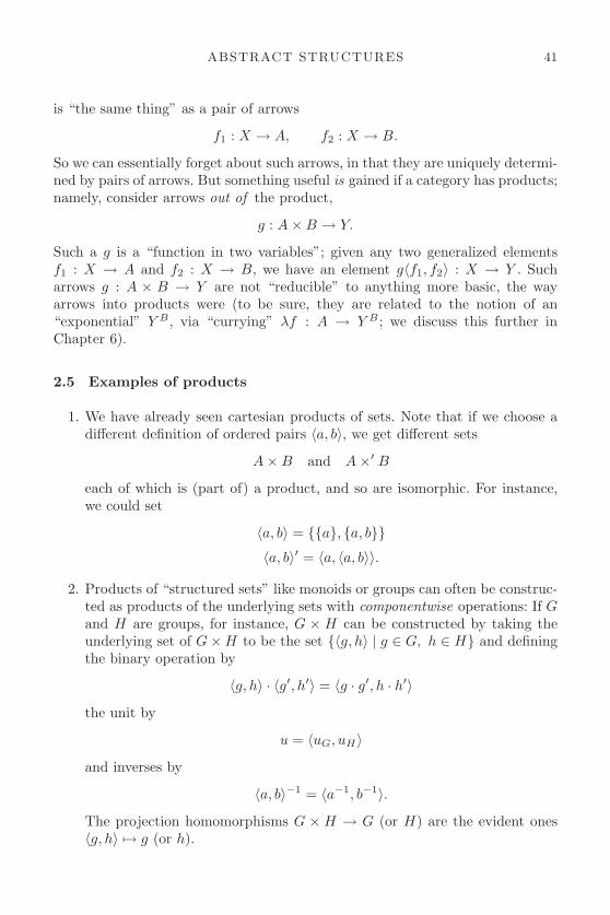
ABSTRACT STRUCTURES 41
is “the same thing” as a pair of arrows
f1 : X → A, f2 : X → B.
So we can essentially forget about such arrows, in that they are uniquely determi-ned by pairs of arrows. But something useful is gained if a category has products;namely, consider arrows out of the product,
g : A×B → Y.
Such a g is a “function in two variables”; given any two generalized elementsf1 : X → A and f2 : X → B, we have an element g〈f1, f2〉 : X → Y . Sucharrows g : A × B → Y are not “reducible” to anything more basic, the wayarrows into products were (to be sure, they are related to the notion of an“exponential” Y B , via “currying” λf : A → Y B; we discuss this further inChapter 6).
2.5 Examples of products
1. We have already seen cartesian products of sets. Note that if we choose adifferent definition of ordered pairs 〈a, b〉, we get different sets
A×B and A×′ B
each of which is (part of) a product, and so are isomorphic. For instance,we could set
〈a, b〉 = {{a}, {a, b}}〈a, b〉′ = 〈a, 〈a, b〉〉.
2. Products of “structured sets” like monoids or groups can often be construc-ted as products of the underlying sets with componentwise operations: If Gand H are groups, for instance, G × H can be constructed by taking theunderlying set of G×H to be the set {〈g, h〉 | g ∈ G, h ∈ H} and definingthe binary operation by
〈g, h〉 · 〈g′, h′〉 = 〈g · g′, h · h′〉the unit by
u = 〈uG, uH〉and inverses by
〈a, b〉−1 = 〈a−1, b−1〉.The projection homomorphisms G × H → G (or H) are the evident ones〈g, h〉 �→ g (or h).

42 CATEGORY THEORY
3. Similarly, for categories C and D, we already defined the category of pairsof objects and arrows,
C×D.
Together with the evident projection functors, this is indeed a product inCat (when C and D are small). (Check this: verify the UMP for the productcategory so defined.)
As special cases, we also get products of posets and of monoids as pro-ducts of categories. (Check this: the projections and unique paired functionare always monotone and so the product of posets, constructed in Cat, isalso a product in Pos, and similarly for Mon.)
4. Let P be a poset and consider a product of elements p, q ∈ P . We musthave projections
p× q ≤ p
p× q ≤ q
and if for any element x,
x ≤ p, and x ≤ q
then we need
x ≤ p× q.
Do you recognize this operation p × q? It is just what is usually calledthe greatest lower bound : p× q = p∧ q. Many other order-theoretic notionsare also special cases of categorical ones, as we shall see later.
5. (For those who know something about Topology.) Let us show that theproduct of two topological spaces X,Y , as usually defined, really is a productin Top, the category of spaces and continuous functions. Thus, suppose wehave spaces X and Y and the product spaces X × Y with its projections
Xp1←− X × Y
p2−→ Y.
Recall that O(X × Y ) is generated by basic open sets of the form U × Vwhere U ∈ O(X) and V ∈ O(Y ), so every W ∈ O(X×Y ) is a union of suchbasic opens.
• Clearly p1 is continuous, since p−11 U = U × Y .
• Given any continuous f1 : Z → X, f2 : Z → Y, let f : Z → X × Y bethe function f = 〈f1, f2〉. We just need to see that f is continuous.

ABSTRACT STRUCTURES 43
• Given any W =⋃
i(Ui × Vi) ∈ O(X × Y ), f−1(W ) =⋃
i f−1(Ui × Vi),so it suffices to show f−1(U × V ) is open. But
f−1(U × V ) = f−1((U × Y ) ∩ (X × V ))
= f−1(U × Y ) ∩ f−1(X × V )
= f−1 ◦ p−11 (U) ∩ f−1 ◦ p−1
2 (V )
= (f1)−1(U) ∩ (f2)−1(V )
where (f1)−1(U) and (f2)−1(V ) are open, since f1 and f2 arecontinuous.
The following diagram concisely captures the situation at hand:
O(Z)
O(X)p−11
�
f−11
�
O(X × Y )
f−1
�.................
�p−12
O(Y )
f−12
�
6. (For those familiar with type theory.) Let us consider the category of typesof the (simply typed) λ-calculus. The λ–calculus is a formalism for thespecification and manipulation of functions, based on the notions of “bin-ding of variables” and functional evaluation. For example, given the realpolynomial expression x2 + 2y, in the λ-calculus one writes λy.x2 + 2y forthe function y �→ x2 + 2y (for each fixed value x), and λxλy.x2 + 2y forthe function-valued function x �→ (y �→ x2 + 2y).
Formally, the λ-calculus consists of
• Types: A×B, A → B, . . . (generated from some basic types)
• Terms:
x, y, z, . . . : A (variables for each type A)
a : A, b : B, . . . (possibly some typed constants)
〈a, b〉 : A×B (a : A, b : B)
fst(c) : A (c : A×B)
snd(c) : B (c : A×B)
ca : B (c : A → B, a : A)
λx.b : A → B (x : A, b : B)

44 CATEGORY THEORY
• Equations:
fst(〈a, b〉) = a
snd(〈a, b〉) = b
〈fst(c), snd(c)〉 = c
(λx.b)a = b[a/x]
λx.cx = c (no x in c)
The relation a ∼ b (usually called βη-equivalence) on terms is defined to bethe equivalence relation generated by the equations, and renaming of boundvariables:
λx.b = λy.b[y/x] (no y in b)
The category of types C(λ) is now defined as follows:
• Objects: the types,
• Arrows A → B: closed terms c : A → B, identified if c ∼ c′,
• Identities: 1A = λx.x (where x : A),
• Composition: c ◦ b = λx.c(bx).
Let us verify that this is a well-defined category:Unit laws:
c ◦ 1B = λx(c((λy.y)x)) = λx(cx) = c
1C ◦ c = λx((λy.y)(cx)) = λx(cx) = c
Associativity:
c ◦ (b ◦ a) = λx(c((b ◦ a)x))
= λx(c((λy.b(ay))x))
= λx(c(b(ax)))
= λx(λy(c(by))(ax))
= λx((c ◦ b)(ax))
= (c ◦ b) ◦ a
This category has binary products. Indeed, given types A and B, let
p1 = λz.fst(z), p2 = λz.snd(z) (z : A×B).

ABSTRACT STRUCTURES 45
And given a and b as in
X
A �p1
a
�A×B
(a, b)
�
.................
p2
� B
b
�
let
(a, b) = λx.〈ax, bx〉.Then
p1 ◦ (a, b) = λx(p1((λy.〈ay, by〉)x))
= λx(p1〈ax, bx〉)= λx(ax)
= a.
Similarly, p2 ◦ (a, b) = b.Finally, if c : X → A×B also has
p1 ◦ c = a, p2 ◦ c = b
then
(a, b) = λx.〈ax, bx〉= λx.〈(p1 ◦ c)x, (p2 ◦ c)x〉= λx.〈(λy(p1(cy)))x, (λy(p2(cy)))x〉= λx.〈(λy((λz.fst(z))(cy)))x, (λy((λz.snd(z))(cy)))x〉= λx.〈λy(fst(cy))x, λy(snd(cy))x〉= λx.〈fst(cx), snd(cx)〉= λx.(cx)
= c.
Remark 2.18. The λ-calculus had another surprising interpretation, namely asa system of notation for proofs in propositional calculus; this is known as the“Curry–Howard” correspondence. Briefly, the idea is that one interprets types aspropositions (with A×B being conjunction and A → B implication) and termsa : A as proofs of the proposition A. The term-forming rules such as
a : A b : B
〈a, b〉 : A×B

46 CATEGORY THEORY
can then be read as annotated rules of inference, showing how to buildup labels for proofs inductively. So, for instance, a natural deduction proofsuch as
[A] [B]A×B
B → (A×B)A → (B → (A×B))
with square brackets indicating cancellation of premisses, is labeled asfollows:
[x : A] [y : B]〈x, y〉 : A×B
λy.〈x, y〉 : B → (A×B)λxλy.〈x, y〉 : A → (B → (A×B))
The final “proof term” λxλy.〈x, y〉 thus records the given proof of the “proposi-tion” A → (B → (A×B)), and a different proof of the same proposition wouldgive a different term.
Although one often speaks of a resulting “isomorphism” between logic andtype theory, what we in fact have here is simply a functor from the category ofproofs in the propositional calculus with conjunction and implication (as definedin example 10 of Section 1.4.), into the category of types of the λ-calculus. Thefunctor will not generally be an isomorphism unless we impose some furtherequations between proofs.
2.6 Categories with products
Let C be a category that has a product diagram for every pair of objects. Supposewe have objects and arrows
A � p1A×A′ p2� A′
B
f
��
q1
B ×B′q2
� B′
f ′
�
with indicated products. Then, we write
f × f ′ : A×A′ → B ×B′

ABSTRACT STRUCTURES 47
for f×f ′ = 〈f ◦p1, f′◦p2〉. Thus, both squares in the following diagram commute:
A � p1A×A′ p2� A′
B
f
��
q1
B ×B′
f × f ′
�
................
q2
� B′
f ′
�
In this way, if we choose a product for each pair of objects, we get a functor
× : C×C → C
as the reader can easily check, using the UMP of the product. A category whichhas a product for every pair of objects is said to have binary products.
We can also define ternary products
A1 ×A2 ×A3
with an analogous UMP (there are three projections pi : A1 × A2 × A3 → Ai,and for any object X and three arrows xi : X → Ai, there is a unique arrowu : X → A1×A2×A3 such that piu = xi for each of the three i’s). Plainly, sucha condition can be formulated for any number of factors.
It is clear, however, that if a category has binary products, then it has allfinite products with two or more factors; for instance, one could set
A×B × C = (A×B)× C
to satisfy the UMP for ternary products. On the other hand, one could insteadhave taken A×(B×C) just as well. This shows that the binary product operationA×B is associative up to isomorphism, for we must have
(A×B)× C ∼= A× (B × C)
by the UMP of ternary products.Observe also that a terminal object is a “nullary” product, that is, a product
of no objects:
Given no objects, there is an object 1 with no maps, and given any otherobject X and no maps, there is a unique arrow
! : X → 1
making nothing further commute.
Similarly, any object A is the unary product of A with itself one time.Finally, one can also define the product of a family of objects (Ci)i∈I indexed
by any set I, by giving a UMP for “I-ary products” analogous to those fornullary, unary, binary, and n-ary products. We leave the precise formulation ofthis UMP as an exercise.

48 CATEGORY THEORY
Definition 2.19. A category C is said to have all finite products, if it has aterminal object and all binary products (and therewith products of any finitecardinality). The category C has all (small) products if every set of objects in Chas a product.
2.7 Hom-sets
In this section, we assume that all categories are locally small.Recall that in any category C, given any objects A and B, we write
Hom(A,B) = {f ∈ C | f : A → B}and call such a set of arrows a Hom-set. Note that any arrow g : B → B′ in Cinduces a function
Hom(A, g) : Hom(A,B) → Hom(A,B′)
(f : A → B) �→ (g ◦ f : A → B → B′)
Thus, Hom(A, g) = g ◦ f ; one sometimes writes g∗ instead of Hom(A, g), so
g∗(f) = g ◦ f.
Let us show that this determines a functor
Hom(A,−) : C → Sets,
called the (covariant) representable functor of A. We need to show that
Hom(A, 1X) = 1Hom(A,X)
and that
Hom(A, g ◦ f) = Hom(A, g) ◦Hom(A, f).
Taking an argument x : A → X, we clearly have
Hom(A, 1X)(x) = 1X ◦ x
= x
= 1Hom(A,X)(x)
and
Hom(A, g ◦ f)(x) = (g ◦ f) ◦ x
= g ◦ (f ◦ x)
= Hom(A, g)(Hom(A, f)(x)).
We will study such representable functors much more carefully later. For now,we just want to see how one can use Hom-sets to give another formulation of thedefinition of products.

ABSTRACT STRUCTURES 49
For any object P , a pair of arrows p1 : P → A and p2 : P → B determine anelement (p1, p2) of the set
Hom(P,A)×Hom(P,B).
Now, given any arrow
x : X → P
composing with p1 and p2 gives a pair of arrows x1 = p1 ◦ x : X → A andx2 = p2 ◦ x : X → B, as indicated in the following diagram:
X
A �p1
x1
�
P
x
�
p2
� B
x2
�
In this way, we have a function
ϑX = (Hom(X, p1),Hom(X, p2)) : Hom(X,P ) → Hom(X,A)×Hom(X,B)
defined byϑX(x) = (x1, x2) (2.1)
This function ϑX can be used to express concisely the condition of being aproduct as follows.
Proposition 2.20. A diagram of the form
A �p1
Pp2
� B
is a product for A and B iff for every object X, the canonical function ϑX givenin (2.1) is an isomorphism,
ϑX : Hom(X,P ) ∼= Hom(X,A)×Hom(X,B).
Proof. Examine the UMP of the product: it says exactly that for every element(x1, x2) ∈ Hom(X,A)×Hom(X,B), there is a unique x ∈ Hom(X,P ) such thatϑX(x) = (x1, x2), that is, ϑX is bijective.
Definition 2.21. Let C, D be categories with binary products. A functor F :C → D is said to preserve binary products if it takes every product diagram
A �p1
A×Bp2
� B in C
to a product diagram
FA �Fp1
F (A×B)Fp2
� FB in D.

50 CATEGORY THEORY
It follows that F preserves products just if
F (A×B) ∼= FA× FB
“canonically,” that is, iff the canonical “comparison arrow”
〈Fp1, Fp2〉 : F (A×B) → FA× FB
in D is an iso.
For example, the forgetful functor U : Mon → Sets preserves binaryproducts.
Corollary 2.22. For any object X in a category C with products, the (covari-ant) representable functor
HomC(X,−) : C → Sets
preserves products.
Proof. For any A,B ∈ C, the foregoing proposition 2.20 says that there is acanonical isomorphism:
HomC(X,A×B) ∼= HomC(X,A)×HomC(X,B)
2.8 Exercises
1. Show that a function between sets is an epimorphism if and onlyif it is surjective. Conclude that the isos in Sets are exactly theepi-monos.
2. Show that in a poset category, all arrows are both monic and epic.3. (Inverses are unique.) If an arrow f : A → B has inverses g, g′ : B → A
(i. e., g ◦ f = 1A and f ◦ g = 1B , and similarly for g′), then g = g′.4. With regard to a commutative triangle,
Af � B
C
g
�h
�
in any category C, show
(a) if f and g are isos (resp. monos, resp. epis), so is h;(b) if h is monic, so is f ;(c) if h is epic, so is g;

ABSTRACT STRUCTURES 51
(d) (by example) if h is monic, g need not be.
5. Show that the following are equivalent for an arrow
f : A → B
in any category:
(a) f is an isomorphism.(b) f is both a mono and a split epi.(c) f is both a split mono and an epi.(d) f is both a split mono and a split epi.
6. Show that a homomorphism h : G → H of graphs is monic just if it isinjective on both edges and vertices.
7. Show that in any category, any retract of a projective object is alsoprojective.
8. Show that all sets are projective (use the axiom of choice).9. Show that the epis among posets are the surjections (on elements), and
that the one-element poset 1 is projective.10. Show that sets, regarded as discrete posets, are projective in the category
of posets (use the foregoing exercises). Give an example of a poset that isnot projective. Show that every projective poset is discrete, that is, a set.Conclude that Sets is (isomorphic to) the “full subcategory” of projectivesin Pos, consisting of all projective posets and all monotone maps betweenthem.
11. Let A be a set. Define an A-monoid to be a monoid M equipped witha function m : A → U(M) (to the underlying set of M). A morphismh : (M,m) → (N,n) of A-monoids is to be a monoid homomorphismh : M → N such that U(h) ◦ m = n (a commutative triangle). Togetherwith the evident identities and composites, this defines a category A-Monof A-monoids.
Show that an initial object in A-Mon is the same thing as a free monoidM(A) on A. (Hint: compare their respective UMPs.)
12. Show that for any Boolean algebra B, Boolean homomorphisms h : B → 2correspond exactly to ultrafilters in B.
13. In any category with binary products, show directly that
A× (B × C) ∼= (A×B)× C.
14. (a) For any index set I, define the product∏
i∈I Xi of an I-indexed familyof objects (Xi)i∈I in a category, by giving a UMP generalizing thatfor binary products (the case I = 2).
(b) Show that in Sets, for any set X the set XI of all functions f : I → Xhas this UMP, with respect to the “constant family” where Xi = X

52 CATEGORY THEORY
for all i ∈ I, and thus
XI ∼=∏i∈I
X.
15. Given a category C with objects A and B, define the category CA,B tohave objects (X,x1, x2), where x1 : X → A, x2 : X → B, and with arrowsf : (X,x1, x2) → (Y, y1, y2) being arrows f : X → Y with y1 ◦ f = x1 andy2 ◦ f = x2.
Show that CA,B has a terminal object just in case A and B have aproduct in C.
16. In the category of types C(λ) of the λ-calculus, determine the productfunctor A,B �→ A × B explicitly. Also show that, for any fixed type A,there is a functor A → (−) : C(λ) → C(λ), taking any type X to A → X.
17. In any category C with products, define the graph of an arrow f : A → Bto be the monomorphism
Γ(f) = 〈1A, f〉 : A � A×B
(Why is this monic?). Show that for C = Sets this determines a functorΓ : Sets → Rel to the category Rel of relations, as defined in the exercisesto Chapter 1. (To get an actual relation R(f) ⊆ A×B, take the image ofΓ(f) : A � A×B.)
18. Show that the forgetful functor U : Mon → Sets from monoids to sets isrepresentable. Infer that U preserves all (small) products.

3
DUALITY
We have seen a few examples of definitions and statements that exhibit a kindof “duality,” like initial and terminal object and epimorphisms and monomor-phisms. We now want to consider this duality more systematically. Despite itsrather trivial first impression, it is indeed a deep and powerful aspect of thecategorical approach to mathematical structures.
3.1 The duality principle
First, let us look again at the formal definition of a category: There are two kindsof things, objects A,B,C and . . . , arrows f, g, h, . . . ; four operations dom(f),cod(f), 1A, g ◦ f ; and these satisfy the following seven axioms:
dom(1A) = A cod(1A) = A
f ◦ 1dom(f) = f 1cod(f) ◦ f = f (3.1)
dom(g ◦ f) = dom(f) cod(g ◦ f) = cod(g)
h ◦ (g ◦ f) = (h ◦ g) ◦ f
The operation “g ◦ f” is only defined where
dom(g) = cod(f),
so a suitable form of this should occur as a condition on each equation containing◦, as in dom(g) = cod(f) ⇒ dom(g ◦ f) = dom(f).
Now, given any sentence Σ in the elementary language of category theory, wecan form the “dual statement” Σ∗ by making the following replacements:
f ◦ g for g ◦ f
cod for dom
dom for cod.
It is easy to see that then Σ∗ will also be a well-formed sentence. Next, supposewe have shown a sentence Σ to entail one Δ, that is, Σ ⇒ Δ, without using anyof the category axioms, then clearly Σ∗ ⇒ Δ∗, since the substituted terms aretreated as mere undefined constants. But now observe that the axioms (3.1) for

54 CATEGORY THEORY
category theory (CT) are themselves “self-dual,” in the sense that we have,
CT∗ = CT.
We therefore have the following duality principle.
Proposition 3.1 (formal duality). For any sentence Σ in the language of cate-gory theory, if Σ follows from the axioms for categories, then so does its dualΣ∗:
CT ⇒ Σ implies CT ⇒ Σ∗
Taking a more conceptual point of view, note that if a statement Σ involvessome diagram of objects and arrows,
Af � B
C
g
�g ◦ f �
then the dual statement Σ∗ involves the diagram obtained from it by reversingthe direction and the order of compositions of arrows.
A � fB
C
g
�
f ◦ g
�
Recalling the opposite category Cop of a category C, we see that an interpre-tation of a statement Σ in C automatically gives an interpretation of Σ∗ inCop.
Now suppose that a statement Σ holds for all categories C. Then it alsoholds in all categories Cop, and so Σ∗ holds in all categories (Cop)op. But sincefor every category C,
(Cop)op = C, (3.2)
we see that Σ∗ also holds in all categories C. We therefore have the followingconceptual form of the duality principle.
Proposition 3.2 (Conceptual duality). For any statement Σ about categories,if Σ holds for all categories, then so does the dual statement Σ∗.
It may seem that only very simple or trivial statements, such as “terminalobjects are unique up to isomorphism” are going to be subject to this sort of

DUALITY 55
duality, but in fact this is far from being so. Categorical duality turns out to bea very powerful and a far-reaching phenomenon, as we shall see. Like the dualitybetween points and lines in projective geometry, it effectively doubles ones “bangfor the buck,” yielding two theorems for every proof.
One way this occurs is that, rather than considering statements about allcategories, we can also consider the dual of an abstract definition of a structureor property of objects and arrows, like “being a product diagram.” The dualstructure or property is arrived at by reversing the order of composition and thewords “domain” and “codomain.” (Equivalently, it results from interpreting theoriginal property in the opposite category.) Section 3.2 provides an example ofthis kind.
3.2 Coproducts
Let us consider the example of products and see what the dual notion must be.First, recall the definition of a product.
Definition 3.3. A diagram Ap1←− P
p2−→ B is a product of A and B, if for anyZ and A
z1←− Zz2−→ B there is a unique u : Z → P with pi ◦ u = zi, all as
indicated in
Z
A �p1
z1
�
P
u
�
.................
p2
� B
z2
�
Now what is the dual statement?A diagram A
q1−→ Qq2←− B is a “dual-product” of A and B if for any Z and
Az1−→ Z
z2←− B there is a unique u : Q → Z with u ◦ qi = zi, all as indicated in
Z
Aq1
�
z1
�
Q
u
�.................
�q2
B
z2
�
Actually, these are called coproducts; the convention is to use the prefix “co-” toindicate the dual notion. We usually write A
i1−→ A+Bi2←− B for the coproduct
and [f, g] for the uniquely determined arrow u : A+ B → Z. The “coprojections”i1 : A → A + B and i2 : B → A + B are usually called injections, even thoughthey need not be “injective” in any sense.

56 CATEGORY THEORY
A coproduct of two objects is therefore exactly their product in the oppositecategory. Of course, this immediately gives lots of examples of coproducts. Butwhat about some more familiar ones?
Example 3.4. In Sets, the coproduct A + B of two sets is their disjoint union,which can be constructed, for example, as
A + B = {(a, 1) | a ∈ A} ∪ {(b, 2) | b ∈ B}
with evident coproduct injections
i1(a) = (a, 1), i2(b) = (b, 2).
Given any functions f and g as in
Z
Ai1
�
f
�
A + B
[f, g]
�.................
�i2
B
g
�
we define
[f, g](x, δ) =
{f(x) δ = 1g(x) δ = 2.
Then, if we have an h with h ◦ i1 = f and h ◦ i2 = g, then for any (x, δ) ∈ A+B,we must have
h(x, δ) = [f, g](x, δ)
as can be easily calculated.
Note that in Sets, every finite set A is a coproduct:
A ∼= 1 + 1 + · · ·+ 1 (n-times)
for n = card(A). This is because a function f : A → Z is uniquely determinedby its values f(a) for all a ∈ A. So we have
A ∼= {a1}+ {an}+ · · ·+ {an}∼= 1 + 1 + · · ·+ 1 (n-times).
In this spirit, we often write simply 2 = 1 + 1, 3 = 1 + 1 + 1, etc.
Example 3.5. If M(A) and M(B) are free monoids on sets A and B, then inMon we can construct their coproduct as
M(A) + M(B) ∼= M(A + B).

DUALITY 57
One can see this directly by considering words over A + B, but it also followsabstractly by using the diagram
N
M(A) �
�
M(A + B)
�.................
� M(B)
�
A
ηA
�
� A + B
ηA+B
�
� B
ηB
�
in which the η’s are the respective insertions of generators. The universal map-ping properties (UMPs) of M(A), M(B), A+B, and M(A+B) then imply thatthe last of these has the required UMP of M(A)+M(B). Note that the set of ele-ments of the coproduct M(A)+M(B) of M(A) and M(B) is not the coproductof the underlying sets, but is only generated by the coproduct of their generators,A + B. We shall consider coproducts of arbitrary, that is, not necessarily free,monoids presently.
The foregoing example says that the free monoid functor M : Sets → Monpreserves coproducts. This is an instance of a much more general phenomenon,which we consider later, related to the fact we have already seen that the forgetfulfunctor U : Mon → Sets is representable and so preserves products.
Example 3.6. In Top, the coproduct of two spaces
X + Y
is their disjoint union with the topology O(X + Y ) ∼= O(X)× O(Y ). Note thatthis follows the pattern of discrete spaces, for which O(X) = P (X) ∼= 2X . Thus,for discrete spaces, we indeed have
O(X + Y ) ∼= 2X+Y ∼= 2X × 2Y ∼= O(X)×O(Y ).
A related fact is that the product of two powerset Boolean algebras P(A)and P(B) is also a powerset, namely of the coproduct of the sets A and B,
P(A)× P(B) ∼= P(A + B).
We leave the verification as an exercise.Coproducts of posets are similarly constructed from the coproducts of the
underlying sets, by “putting them side by side.” What about “rooted” posets,that is, posets with a distinguished initial element 0? In the category Pos0 ofsuch posets and monotone maps that preserve 0, one constructs the coproduct

58 CATEGORY THEORY
of two such posets A and B from the coproduct A + B in the category Pos ofposets, by “identifying” the two different 0s,
A+ Pos0B = (A+ PosB)/“0A = 0B”.
We shall soon see how to describe such identifications (quotients of equivalencerelations) as “coequalizers.”
Example 3.7. In a fixed poset P , what is a coproduct of two elements p, q ∈ P ?We have
p ≤ p + q and q ≤ p + q
and if
p ≤ z and q ≤ z
then
p + q ≤ z.
So p + q = p ∨ q is the join, or “least upper bound,” of p and q.
Example 3.8. In the category of proofs of a deductive system of logic of example10, Section 1.4, the usual natural deduction rules of disjunction introduction andelimination give rise to coproducts. Specifically, the introduction rules,
ϕ
ϕ ∨ ψ
ψ
ϕ ∨ ψ
determine arrows i1 : ϕ → ϕ ∨ ψ and i2 : ψ → ϕ ∨ ψ, and the elimination rule,
ϕ ∨ ψ
[ϕ]...ϑ
[ψ]...ϑ
ϑ
turns a pair of arrows p : ϕ → ϑ and q : ψ → ϑ into an arrow [p, q] : ϕ ∨ ψ → ϑ.The required equations,
[p, q] ◦ i1 = p [p, q] ◦ i2 = q (3.3)
will evidently not hold, however, since we are taking identity of proofs as identityof arrows. In order to get coproducts, then, we need to “force” these equations tohold by passing to equivalence classes of proofs, under the equivalence relationgenerated by these equations, together with the complementary one,
[r ◦ i1, r ◦ i2] = r (3.4)
for any r : A + B → C. (The intuition behind these identifications is that oneshould equate proofs which become the same when one omits such “detours.”)

DUALITY 59
In the new category with equivalence classes of proofs as arrows, the arrow [p, q]will also be the unique one satisfying (3.3), so that ϕ ∨ ψ indeed becomes acoproduct.
Closely related to this example (via the Curry–Howard correspondence ofremark 2.18) are the sum types in the λ-calculus, as usually formulated usingcase terms; these are coproducts in the category of types defined in Section 2.5.
Example 3.9. Two monoids A,B have a coproduct of the form
A + B = M(|A|+ |B|)/ ∼where, as before, the free monoid M(|A|+|B|) is strings (words) over the disjointunion |A| + |B| of the underlying sets—that is, the elements of A and B—andthe equivalence relation v ∼ w is the least one containing all instances of thefollowing equations:
(. . . x uA y . . .) = (. . . x y . . .)
(. . . x uB y . . .) = (. . . x y . . .)
(. . . a a′ . . .) = (. . . a ·A a′ . . .)
(. . . b b′ . . .) = (. . . b ·B b′ . . .).
(If you need a refresher on quotienting a set by an equivalence relation, skipahead and read the beginning of Section 3.4 now.) The unit is, of course, theequivalence class [−] of the empty word (which is the same as [uA] and [uB ]).Multiplication of equivalence classes is also as expected, namely
[x . . . y] · [x′ . . . y′] = [x . . . yx′ . . . y′].
The coproduct injections iA : A → A + B and iB : B → A + B are simply
iA(a) = [a], iB(b) = [b],
which are now easily seen to be homomorphisms. Given any homomorphismsf : A → M and g : B → M into a monoid M , the unique homomorphism
[f, g] : A + B −→ M
is defined by first extending the function [|f |, |g|] : |A|+ |B| → |M | to one [f, g]′
on the free monoid M(|A|+ |B|),
|A|+ |B| [|f |, |g|]� |M |
M(|A|+ |B|) [f, g]′ � M
M(|A|+ |B|)/∼��
[f, g]......
............
............
...........�

60 CATEGORY THEORY
and then observing that [f, g]′ “respects the equivalence relation ∼,” in the sensethat if v ∼ w in M(|A| + |B|), then [f, g]′(v) = [f, g]′(w). Thus, the map [f, g]′
extends to the quotient to yield the desired map [f, g] : M(|A|+ |B|)/∼ −→ M .(Why is this homomorphism the unique one h : M(|A| + |B|)/∼ −→ M withhiA = f and hiB = g ?) Summarizing, we thus have
A + B ∼= M(|A|+ |B|)/∼ .
This construction also works to give coproducts in Groups, where it isusually called the free product of A and B and written A ⊕ B, as well as manyother categories of “algebras,” that is, sets equipped with operations. Again, asin the free case, the underlying set of A + B is not the coproduct of A and B assets (the forgetful functor Mon → Sets does not preserve coproducts).
Example 3.10. For abelian groups A,B, the free product A ⊕ B need not beabelian. One could, of course, take a further quotient of A⊕B to get a copro-duct in the category Ab of abelian groups, but there is a more convenient (andimportant) presentation, which we now consider.
Since the words in the free product A⊕B must be forced to satisfy the furthercommutativity conditions
(a1b1b2a2 . . .) ∼ (a1a2 . . . b1b2 . . .)
we can shuffle all the a’s to the front, and the b’s to the back, of the words. But,furthermore, we already have
(a1a2 . . . b1b2 . . .) ∼ (a1 + a2 + · · ·+ b1 + b2 + · · · ).Thus, we in effect have pairs of elements (a, b). So we can take the product setas the underlying set of the coproduct
|A + B| = |A×B|.As inclusions, we use the homomorphisms
iA(a) = (a, 0B)
iB(b) = (0A, b).
Then, given any homomorphisms Af→ X
g← B, we let [f, g] : A + B → X bedefined by
[f, g](a, b) = f(a) +X g(b)
which can easily be seen to do the trick (exercise!).
Moreover, not only can the underlying sets be the same, the product andcoproduct of abelian groups are actually isomorphic as groups.
Proposition 3.11. In the category Ab of abelian groups, there is a canonicalisomorphism between the binary coproduct and product,
A + B ∼= A×B.

DUALITY 61
Proof. To define an arrow ϑ : A+ B → A×B, we need one A → A×B (and oneB → A×B), so we need arrows A → A and A → B (and B → A and B → B).For these, we take 1A : A → A and the zero homomorphism 0B : A → B (and0A : B → A and 1B : B → B). Thus, all together, we get
ϑ = [〈1A, 0B〉, 〈0A, 1B〉] : A + B → A×B.
Then given any (a, b) ∈ A + B, we have
ϑ(a, b) = [〈1A, 0B〉, 〈0A, 1B〉](a, b)
= 〈1A, 0B〉(a) + 〈0A, 1B〉(b)= (1A(a), 0B(a)) + (0A(b), 1B(b))
= (a, 0B) + (0A, b)
= (a + 0A, 0B + b)
= (a, b).
This fact was first observed by Mac Lane, and it was shown to lead to abinary operation of addition on parallel arrows f, g : A → B between abe-lian groups (and related structures like modules and vector spaces). In fact,the group structure of a particular abelian group A can be recovered from thisoperation on arrows into A. More generally, the existence of such an addition ope-ration on arrows can be used as the basis of an abstract description of categorieslike Ab, called “abelian categories,” which are suitable for axiomatic homologytheory.
Just as with products, one can consider the empty coproduct, which is aninitial object 0, as well as coproducts of several factors, and the coproduct oftwo arrows,
f + f ′ : A + A′ → B + B′
which leads to a coproduct functor + : C × C → C on categories C withbinary coproducts. All of these facts follow simply by duality; that is, by consi-dering the dual notions in the opposite category. Similarly, we have the followingproposition.
Proposition 3.12. Coproducts are unique up to isomorphism.
Proof. Use duality and the fact that the dual of “isomorphism” is “isomorphism.”
In just the same way, one also shows that binary coproducts are associative upto isomorphism, (A + B) + C ∼= A + (B + C).
Thus is general, in the future it will suffice to introduce new notions once andthen simply observe that the dual notions have analogous (but dual) properties.Sections 3.3 and 3.4 give another example of this sort.

62 CATEGORY THEORY
3.3 Equalizers
In this section, we consider another abstract characterization; this time a com-mon generalization of the kernel of a homomorphism and an equationally defined“variety,” like the set of zeros of a real-valued function—as well as set theory’saxiom of separation.
Definition 3.13. In any category C, given parallel arrows
Af �
g� B
an equalizer of f and g consists of an object E and an arrow e : E → A, universalsuch that
f ◦ e = g ◦ e.
That is, given any z : Z → A with f ◦ z = g ◦ z, there is a unique u : Z → Ewith e ◦ u = z, all as in the diagram
Ee � A
f �
g� B
Z
u
�.................
z
�
Let us consider some simple examples.
Example 3.14. Suppose we have the functions f, g : R2 ⇒ R, where
f(x, y) = x2 + y2
g(x, y) = 1
and we take the equalizer, say in Top. This is the subspace,
S = {(x, y) ∈ R2 |x2 + y2 = 1} ↪→ R2,
that is, the unit circle in the plane. For, given any “generalized element” z : Z →R2, we get a pair of such “elements” z1, z2 : Z → R just by composing with thetwo projections, z = 〈z1, z2〉, and for these we then have
f(z) = g(z) iff z12 + z2
2 = 1
iff “〈z1, z2〉 = z ∈ S”,

DUALITY 63
where the last line really means that there is a factorization z = z◦i of z throughthe inclusion i : S ↪→ R2, as indicated in the following diagram:
S ⊂i � R2
x2 + y2�
1� R
Z
z
�.................
z
�Since the inclusion i is monic, such a factorization, if it exists, is necessarilyunique, and thus S ↪→ R2 is indeed the equalizer of f and g.
Example 3.15. Similarly, in Sets, given any functions f, g : A ⇒ B, theirequalizer is the inclusion into A of the equationally defined subset
{x ∈ A | f(x) = g(x)} ↪→ A.
The argument is essentially the same as the one just given.Let us pause here to note that in fact, every subset U ⊆ A is of this “equatio-
nal” form, that is, every subset is an equalizer for some pair of functions. Indeed,one can do this in a very canonical way. First, let us put
2 = {�,⊥},
thinking of it as the set of “truth values.” Then consider the characteristicfunction
χU : A → 2,
defined for x ∈ A by
χU (x) =
{� x ∈ U
⊥ x /∈ U.
Thus, we have
U = {x ∈ A |χU (x) = �}.
So the following is an equalizer:
U � A�! �
χU
� 2
where �! = �◦! : U!→ 1 �→ 2.
Moreover, for every function,
ϕ : A → 2

64 CATEGORY THEORY
we can form the “variety” (i.e., equational subset)
Vϕ = {x ∈ A |ϕ(x) = �}as an equalizer, in the same way. (Thinking of ϕ as a “propositional function”defined on A, the subset Vϕ ⊆ A is the “extension” of ϕ provided by the axiomof separation.)
Now, it is easy to see that these operations χU and Vϕ are mutually inverse:
VχU= {x ∈ A |χU (x) = �}= {x ∈ A |x ∈ U}= U
for any U ⊆ A, and given any ϕ : A → 2,
χVϕ(x) =
{� x ∈ Vϕ
⊥ x /∈ Vϕ
={� ϕ(x) = �⊥ ϕ(x) = ⊥
= ϕ(x).
Thus, we have the familiar isomorphism
Hom(A, 2) ∼= P (A),
mediated by taking equalizers.
The fact that equalizers of functions can be taken to be subsets is a specialcase of a more general phenomenon.
Proposition 3.16. In any category, if e : E → A is an equalizer of some pairof arrows, then e is monic.
Proof. Consider the diagram
Ee � A
f �
g� B
Z
x
�
y
�
z
�
in which we assume e is the equalizer of f and g. Supposing ex = ey, we wantto show x = y. Put z = ex = ey. Then fz = fex = gex = gz, so there is aunique u : Z → E such that eu = z. So from ex = z and ey = z it follows thatx = u = y.
Example 3.17. In many other categories, such as posets and monoids, the equa-lizer of a parallel pair of arrows f, g : A ⇒ B can be constructed by taking the

DUALITY 65
equalizer of the underlying functions as above, that is, the subset A(f = g) ⊆ Aof elements x ∈ A where f and g agree, f(x) = g(x), and then restricting thestructure of A to A(f = g). For instance, in posets one takes the ordering fromA restricted to this subset A(f = g), and in topological spaces one takes thesubspace topology.
In monoids, the subset A(f = g) is then also a monoid with the operationsfrom A, and the inclusion is therefore a homomorphism. This is so becausef(uA) = uB = g(uA), and if f(a) = g(a) and f(a′) = g(a′), then f(a · a′) =f(a) · f(a′) = g(a) · g(a′) = g(a · a′). Thus, A(f = g) contains the unit and isclosed under the product operation.
In abelian groups, for instance, one has an alternate description of theequalizer, using the fact that,
f(x) = g(x) iff (f − g)(x) = 0.
Thus, the equalizer of f and g is the same as that of the homomorphism (f − g)and the zero homomorphism 0 : A → B, so it suffices to consider equalizersof the special form A(h, 0) � A for arbitrary homomorphisms h : A → B.This subgroup of A is called the kernel of h, written ker(h). Thus, we have theequalizer
ker(f − g) ⊂ � Af �
g� B.
The kernel of a homomorphism is of fundamental importance in the study ofgroups, as we consider further in Chapter 4.
3.4 Coequalizers
A coequalizer is a generalization of a quotient by an equivalence relation, so letus begin by reviewing that notion, which we have already made use of severaltimes. Recall first that an equivalence relation on a set X is a binary relationx ∼ y, which is
reflexive: x ∼ x,symmetric: x ∼ y implies y ∼ x,transitive: x ∼ y and y ∼ z implies x ∼ z.
Given such a relation, define the equivalence class [x] of an element x ∈ X by
[x] = {y ∈ X |x ∼ y}.
The various different equivalence classes [x] then form a partition of X, in thesense that every element y is in exactly one of them, namely [y] (prove this!).
One sometimes thinks of an equivalence relation as arising from the equivalentelements having some property in common (like being the same color). One can

66 CATEGORY THEORY
then regard the equivalence classes [x] as the properties and in that sense as“abstract objects” (the colors red, blue, etc., themselves). This is sometimesknown as “definition by abstraction,” and it describes, for example, the waythat the real numbers can be constructed from Cauchy sequences of rationals orthe finite cardinal numbers from finite sets.
The set of all equivalence classes
X/∼ = {[x] |x ∈ X}may be called the quotient of X by ∼. It is used in place of X when one wants to“abstract away” the difference between equivalent elements x ∼ y, in the sensethat in X/∼ such elements (and only such) are identified, since
[x] = [y] iff x ∼ y.
Observe that the quotient mapping,
q : X −→ X/∼taking x to [x] has the property that a map f : X → Y extends along q,
Xq � X/∼
Y�
................f
�
just in case f respects the equivalence relation, in the sense that x ∼ y impliesf(x) = f(y).
Now let us consider the notion dual to that of equalizer, namely that of acoequalizer.
Definition 3.18. For any parallel arrows f, g : A → B in a category C, acoequalizer consists of Q and q : B → Q, universal with the property qf = qg,as in
Af �
g� B
q � Q
Z .
u
�
................z
�
That is, given any Z and z : B → Z, if zf = zg, then there exists a uniqueu : Q → Z such that uq = z.
First, observe that by duality, we know that such a coequalizer q in a categoryC is an equalizer in Cop, hence monic by proposition 3.16, and so epic in C.

DUALITY 67
Proposition 3.19. If q : B → Q is a coequalizer of some pair of arrows, thenq is epic.
We can therefore think of a coequalizer q : B � Q as a “collapse” of B by“identifying” all pairs f(a) = g(a) (speaking as if there were such “elements”a ∈ A). Moreover, we do this in the “minimal” way, that is, disturbing B as littleas possible, in that one can always map Q to anything else Z in which all suchidentifications hold.
Example 3.20. Let R ⊆ X×X be an equivalence relation on a set X, and considerthe diagram
Rr1 �
r2
� X
where the r’s are the two projections of the inclusion R ⊆ X ×X,
R
X �p1
r1
�
X ×X�
∩
p2
� X
r2
�
The quotient projectionπ : X −→ X/R
defined by x �→ [x] is then a coequalizer of r1 and r2. For given an f : X → Yas in
Rr1 �
r2
� Xπ � X/R
Y
f
�
..................
f�
there exists a function f such that
fπ(x) = f(x)
whenever f respects R in the sense that (x, x′) ∈ R implies f(x) = f(x′), asalready noted. But this condition just says that f ◦r1 = f ◦r2, since f ◦r1(x, x′) =f(x) and f ◦ r2(x, x′) = f(x′) for all (x, x′) ∈ R. Moreover, if it exists, such afunction f , is then necessarily unique, since π is an epimorphism.
The coequalizer in Sets of an arbitrary parallel pair of functions f ·g : A ⇒ Bcan be constructed by quotienting B by the equivalence relation generated bythe equations f(x) = g(x) for all x ∈ A. We leave the details as an exercise.

68 CATEGORY THEORY
Example 3.21. In example 3.6, we considered the coproduct of rooted posets Pand Q by first making P + Q in posets and then “identifying” the resulting twodifferent 0-elements 0P and 0Q (i.e., the images of these under the respectivecoproduct inclusions. We can now describe this “identification” as a coequalizer,taken in posets,
10P �
0Q
� P + Q � P + Q/(0P = 0Q).
This clearly has the right UMP to be the coproduct in rooted posets.In topology one also often makes “identifications” of points (as in making
the circle out of the interval by identifying the endpoints), of subspaces (makingthe torus from a region in the plane, etc.). These and many similar “gluing”constructions can be described as coequalizers. In Top, the coequalizer of aparallel pair of maps f, g : X → Y can be constructed as a quotient space of Y(see the exercises).
Example 3.22. Presentations of algebrasConsider any category of “algebras,” that is, sets equipped with operations (offinite arity), such as monoids or groups. We shall show later that such a categoryhas free algebras for all sets and coequalizers for all parallel pairs of arrows (seethe exercises for a proof that monoids have coequalizers). We can use these todetermine the notion of a presentation of an algebra by generators and relations.For example, suppose we are given
Generators: x, y, z
Relations: xy = z, y2 = 1. (3.5)
To build an algebra on these generators and satisfying these relations, start withthe free algebra,
F (3) = F (x, y, z),
and then “force” the relation xy = z to hold by taking a coequalizer of the maps
F (1)xy�
z� F (3)
q � Q.
We use the fact that maps F (1) → A correspond to elements a ∈ A by v �→ a,where v is the single generator of F (1). Now similarly, for the equation y2 = 1,take the coequalizer
F (1)q(y2)�q(1)
� Q � Q′.
These two steps can actually be done simultaneously. Let
F (2) = F (1) + F (1)

DUALITY 69
F (2)f �
g� F (3)
where f = [xy, y2] and g = [z, 1]. The coequalizer q : F (3) → Q of f and g then“forces” both equations to hold, in the sense that in Q, we have
q(x)q(y) = q(z), q(y)2 = 1.
Moreover, no other relations among the generators hold in Q except those requi-red to hold by the stipulated equations. To make the last statement precise,observe that given any algebra A and any three elements a, b, c ∈ A such thatab = c and b2 = 1, by the UMP of Q there is a unique homomorphism u : Q → Asuch that
u(x) = a, u(y) = b, u(z) = c.
Thus, any other equation that holds among the generators in Q will also holdin any other algebra in which the stipulated equations (3.5) hold, since thehomomorphism u also preserves equations. In this sense, Q is the “universal”algebra with three generators satisfying the stipulated equations; as may bewritten suggestively in the form
Q ∼= F (x, y, z)/(xy = z, y2 = 1).
Generally, given a finite presentation
Generators: g1, . . . , gn
Relations: l1 = r1, . . . , lm = rm (3.6)
(where the li and ri are arbitrary terms built from the generators and theoperations) the algebra determined by that presentation is the coequalizer
F (m)l �
r� F (n) � Q = F (n)/(l = r)
where l = [l1, . . . , lm] and r = [r1, . . . , rm]. Moreover, any such coequalizer bet-ween (finite) free algebras can clearly be regarded as a (finite) presentation bygenerators and relations. Algebras that can be given in this way are said to befinitely presented.
Warning 3.23. Presentations are not unique. One may well have two differentpresentations F (n)/(l = r) and F (n′)/(l′ = r′) by generators and relations ofthe same algebra,
F (n)/(l = r) ∼= F (n′)/(l′ = r′).
For instance, given F (n)/(l = r) just add a new generator gn+1 and the newrelation gn = gn+1. In general, there are many different ways of presenting agiven algebra, just like there are many ways of axiomatizing a logical theory.

70 CATEGORY THEORY
We did not really make use of the finiteness condition in the foregoing consi-derations. Indeed, any sets of generators G and relations R give rise to an algebrain the same way, by taking the coequalizer
F (R)r1�
r2
� F (G) � F (G)/(r1 = r2).
In fact, every algebra can be “presented” by generators and relations in thissense, that is, as a coequalizer of maps between free algebras. Specifically, wehave the following proposition for monoids, an analogous version of which alsoholds for groups and other algebras.
Proposition 3.24. For every monoid M there are sets R and G and acoequalizer diagram,
F (R)r1�
r2
� F (G) � M
with F (R) and F (G) free; thus, M ∼= F (G)/(r1 = r2).
Proof. For any monoid N , let us write TN = M(|N |) for the free monoid onthe set of elements of N (and note that T is therefore a functor). There is ahomomorphism,
π : TN → N
π(x1, . . . , xn) = x1 · . . . · xn
induced by the identity 1|N | : |N | → |N | on the generators. (Here we are writingthe elements of TN as tuples (x1, . . . , xn) rather than strings x1 . . . xn for clarity.)Applying this construction twice to a monoid M results in the arrows π and εin the following diagram:
T 2Mε �
μ� TM
π� M (3.7)
where T 2M = TTM and μ = Tπ. Explicitly, the elements of T 2M are tup-les of tuples of elements of M , say ((x1, . . . , xn), . . . , (z1, . . . , zm)), and thehomomorphisms ε and μ have the effect:
ε((x1, . . . , xn), . . . , (z1, . . . , zm)) = (x1, . . . , xn, . . . , z1, . . . , zm)
μ((x1, . . . , xn), . . . , (z1, . . . , zm)) = (x1 · . . . · xn, . . . , z1 · . . . · zm)
Briefly, ε uses the multiplication in TM and μ uses that in M .Now clearly π ◦ ε = π ◦ μ. We claim that (3.7) is a coequalizer of monoids.
To that end, suppose we have a monoid N and a homomorphism h : TM → N

DUALITY 71
with hε = hμ. Then for any tuple (x, . . . , z), we have
h(x, . . . , z) = hε((x, . . . , z))
= hμ((x, . . . , z))
= h(x · . . . · z).
(3.8)
Now define h = h ◦ i, where i : |M | → |TM | is the insertion of generators, asindicated in the following:
T 2ε �
μ� TM
π ��.......
i......... M
N
h ◦ i
�
h�
We then have
hπ(x, . . . , z) = hiπ(x, . . . , z)
= h(x · . . . · z)
= h(x, . . . , z) by (3.8).
We leave it as an easy exercise for the reader to show that h is a homomorphism.
3.5 Exercises
1. In any category C, show that
Ac1
� C �c2
B
is a coproduct diagram just if for every object Z, the map
Hom(C,Z) −→ Hom(A,Z)×Hom(B,Z)
f �−→ 〈f ◦ c1, f ◦ c2〉
is an isomorphism. Do this by using duality, taking the corresponding factabout products as given.
2. Show in detail that the free monoid functor M preserves coproducts: forany sets A,B,
M(A) + M(B) ∼= M(A + B) (canonically).
Do this as indicated in the text by using the UMPs of the coproducts A+Band M(A) + M(B) and of free monoids.

72 CATEGORY THEORY
3. Verify that the construction given in the text of the coproduct of monoidsA + B as a quotient of the free monoid M(|A|+ |B|) really is a coproductin the category of monoids.
4. Show that the product of two powerset Boolean algebras P(A) and P(B)is also a powerset, namely of the coproduct of the sets A and B,
P(A)× P(B) ∼= P(A + B).
(Hint: determine the projections π1 : P(A + B) → P(A) and π2 : P(A +B) → P(B), and check that they have the UMP of the product.)
5. Consider the category of proofs of a natural deduction system with dis-junction introduction and elimination rules. Identify proofs under theequations
[p, q] ◦ i1 = p, [p, q] ◦ i2 = q
[r ◦ i1, r ◦ i2] = r
for any p : A → C, q : B → C, and r : A + B → C. By passing toequivalence classes of proofs with respect to the equivalence relation gene-rated by these equations (i.e., two proofs are equivalent if you can get onefrom the other by removing all such “detours”). Show that the resultingcategory does indeed have coproducts.
6. Verify that the category of monoids has all equalizers and finite products,then do the same for abelian groups.
7. Show that in any category with coproducts, the coproduct of twoprojectives is again projective.
8. Dualize the notion of projectivity to define an injective object in a category.Show that a map of posets is monic iff it is injective on elements. Giveexamples of a poset that is injective and one that is not injective.
9. Complete the proof of proposition 3.24 in the text by showing that h isindeed a homomorphism.
10. In the proof of proposition 3.24 in the text it is shown that any monoidM has a specific presentation T 2M ⇒ TM → M as a coequalizer of freemonoids. Show that coequalizers of this particular form are preserved bythe forgetful functor Mon → Sets.
11. Prove that Sets has all coequalizers by constructing the coequalizer of aparallel pair of functions,
Af �
g� B � Q = B/(f = g)
by quotienting B by a suitable equivalence relation R on B, generated bythe pairs (f(x), g(x)) for all x ∈ A. (Define R to be the intersection of allequivalence relations on B containing all such pairs.)

DUALITY 73
12. Verify the coproduct–coequalizer construction mentioned in the text forcoproducts of rooted posets, that is, posets with a least element 0 andmonotone maps preserving 0. Specifically, show that the coproduct P +0 Qof two such posets can be constructed as a coequalizer in posets,
10P �
0Q
� P + Q � P +0 Q.
(You may assume as given the fact that the category of posets has allcoequalizers.)
13. Show that the category of monoids has all coequalizers as follows.1. Given any pair of monoid homomorphisms f, g : M → N , show that thefollowing equivalence relations on N agree:
(a) n ∼ n′ ⇔ for all monoids X and homomorphisms h : N → X, one hashf = hg implies hn = hn′,
(b) the intersection of all equivalence relations ∼ on N satisfying fm ∼ gmfor all m ∈ M as well as
n ∼ n′ and m ∼ m′ ⇒ n ·m ∼ n′ ·m′
2. Taking ∼ to be the equivalence relation defined in (1), show that thequotient set N/∼ is a monoid under [n] · [m] = [n ·m], and the projectionN → N/∼ is the coequalizer of f and g.
14. Consider the following category of sets:
(a) Given a function f : A → B, describe the equalizer of the functionsf ◦ p1, f ◦ p2 : A × A → B as a (binary) relation on A and show thatit is an equivalence relation (called the kernel of f).
(b) Show that the kernel of the quotient A → A/R by an equivalencerelation R is R itself.
(c) Given any binary relation R ⊆ A × A, let 〈R〉 be the equivalencerelation on A generated by R (the least equivalence relation on Acontaining R). Show that the quotient A → A/〈R〉 is the coequalizerof the two projections R ⇒ A.
(d) Using the foregoing, show that for any binary relation R on a set A,one can characterize the equivalence relation 〈R〉 generated by R asthe kernel of the coequalizer of the two projections of R.
15. Construct coequalizers in Top as follows. Given a parallel pair of mapsf, g : X ⇒ Y , make a quotient space q : Y → Q by (i) taking the coequa-lizer of |f | and |g| in Sets to get the function |q| : |Y | → |Q|, then (ii)equip |Q| with the quotient topology, under which a set V ⊆ Q is open iffq−1(V ) ⊆ Y is open. This is plainly the finest topology on |Q| that makesthe projection |q| continuous.

This page intentionally left blank

4
GROUPS AND CATEGORIES
This chapter is devoted to some of the various connections between groups andcategories. If you already know the basic group theory covered here, then thisgives you some insight into the categorical constructions we have learned so far;and if you do not know it yet, then you learn it now as an application of categorytheory. We focus on three different aspects of the relationship between categoriesand groups:
1. groups in a category,2. the category of groups,3. groups as categories.
4.1 Groups in a category
As we have already seen, the notion of a group arises as an abstraction of theautomorphisms of an object. In a specific, concrete case, a group G may thusconsist of certain arrows g : X → X for some object X in a category C,
G ⊆ HomC(X,X)
But the abstract group concept can also be described directly as an object in acategory, equipped with a certain structure. This more subtle notion of a “groupin a category” also proves to be quite useful.
Let C be a category with finite products. The notion of a group in Cessentially generalizes the usual notion of a group in Sets.
Definition 4.1. A group in C consists of objects and arrows as so:
G×Gm � G � i
G
1
u
�

76 CATEGORY THEORY
satisfying the following conditions:
1. m is associative, that is, the following commutes:
(G×G)×G∼= � G× (G×G)
G×G
m× 1
�G×G
1×m
�
G
m�
m�
where ∼= is the canonical associativity isomorphism for products.2. u is a unit for m, that is, both triangles in the following commute:
G〈u, 1G〉� G×G
G×G
〈1G, u〉
�
m� G
m
�1G
�
where we write u for the “constant arrow” u! : G!→ 1 u→ G.
3. i is an inverse with respect to m, that is, both sides of the followingcommute:
G×G � ΔG
Δ � G×G
G×G
1G × i
�
m� G
u
��
mG×G
i× 1G
�
where Δ = 〈1G, 1G〉.
Note that the requirement that these diagrams commute is equivalent to themore familiar condition that, for all (generalized) elements,
x, y, z : Z → G

GROUPS AND CATEGORIES 77
the following equations hold:
m(m(x, y), z) = m(x,m(y, z))
m(x, u) = x = m(u, x)
m(x, ix) = u = m(ix, x)
Definition 4.2. A homomorphism h : G → H of groups in C consists of anarrow in C,
h : G → H
such that
1. h preserves m:
G×Gh× h� H ×H
G
m
�
h� H
m
�
2. h preserves u:
Gh � H
1
u
�
u
�
3. h preserves i:
Gh � H
G
i
�
h� H
i
�
With the evident identities and composites, we thus have a category of groupsin C, denoted by
Group(C)
Example 4.3. The idea of an internal group in a category captures the familiarnotion of a group with additional structure.

78 CATEGORY THEORY
• A group in the usual sense is a group in the category Sets.
• A topological group is a group in Top, the category of topological spaces.
• A (partially) ordered group is a group in the category Pos of posets (in thiscase, the inverse operation is usually required to be order-reversing, thatis, of the form i : Gop → G).
For example, the real numbers R under addition are a topological and anordered group, since the operations of addition x + y and additive inverse −xare continuous and order-preserving (resp. reversing). They are a topological“semigroup” under multiplication x · y as well, but the multiplicative inverseoperation 1/x is not continuous (or even defined!) at 0.
Example 4.4. Suppose we have a group G in the category Groups of groups.So G is a group equipped with group homomorphisms m : G × G → G, etc.as in definition 4.1. Let us take this apart in more elementary terms. Write themultiplication of the group G, that is, on the underlying set |G|, as x◦y and writethe homomorphic multiplication m as x � y. That the latter is a homomorphismfrom the product group G×G to G says in particular that, for all g, h ∈ G×Gwe have m(g ◦ h) = m(g) ◦ m(h). Recalling that g = (g1, g2), h = (h1, h2) andmultiplication ◦ on G×G is pointwise, this then comes to the following:
(g1 ◦ h1) � (g2 ◦ h2) = (g1 � g2) ◦ (h1 � h2) (4.1)
Write 1◦ for the unit with respect to ◦ and 1� for the unit of �. The followingproposition is called the “Eckmann–Hilton argument,” and was first used inhomotopy theory.
Proposition 4.5. Given any set G equipped with two binary operations ◦, � :G×G → G with units 1◦ and 1�, respectively and satisfying (4.1), the followinghold.
1. 1◦ = 1�.2. ◦ = �.3. The operation ◦ = � is commutative.
Proof. First, we have
1◦ = 1◦ ◦ 1◦
= (1◦ � 1�) ◦ (1� � 1◦)
= (1◦ ◦ 1�) � (1� ◦ 1◦)
= 1� � 1�
= 1�.
Thus, let us write 1◦ = 1 = 1�. Next, we have,
x ◦ y = (x � 1) ◦ (1 � y) = (x ◦ 1) � (1 ◦ y) = x � y.

GROUPS AND CATEGORIES 79
Thus, let us write x ◦ y = x · y = x � y. Finally, we have
x · y = (1 · x) · (y · 1) = (1 · y) · (x · 1) = y · x.
We therefore have the following.
Corollary 4.6. The groups in the category of groups are exactly the abeliangroups.
Proof. We have just shown that a group in Groups is necessarily abelian,so it just remains to see that any abelian group admits homomorphic groupoperations. We leave this as an easy exercise.
Remark 4.7. Note that we did not really need the full group structure in thisargument. Indeed, the same result holds for monoids in the category of monoids:these are exactly the commutative monoids.
Example 4.8. A further example of an internal algebraic structure in a categoryis provided by the notion of a (strict) monoidal category.
Definition 4.9. A strict monoidal category is a category C equipped with abinary operation ⊗ : C×C → C which is functorial and associative,
A⊗ (B ⊗ C) = (A⊗B)⊗ C, (4.2)
together with a distinguished object I that acts as a unit,
I ⊗ C = C = C ⊗ I. (4.3)
A strict monoidal category is exactly the same thing as a monoid in Cat.Examples where the underlying category is a poset P include both the meet x∧yand join x ∨ y operations, with terminal object 1 and initial object 0 as units,respectively (assuming P has these structures), as well as the poset End(P ) ofmonotone maps f : P → P , ordered pointwise, with composition g ◦ f as ⊗ and1P as unit. A discrete monoidal category, that is, one with a discrete underlyingcategory, is obviously just a regular monoid (in Sets), while a monoidal categorywith only one object is a monoidal monoid, and thus exactly a commutativemonoid, by the foregoing remark 4.7.
More general strict monoidal categories, that is, ones having a proper categorywith many objects and arrows, are rather less common—not for a paucity ofsuch structures, but because the required equations (4.2) and (4.3) typicallyhold only “up to isomorphism.” This is so, for example, for products A×B andcoproducts A + B, as well as many other operations like tensor products A⊗Bof vector spaces, modules, algebras over a ring, etc. (the category of proofs inlinear logic provides more examples). We return to this more general notion ofa (not necessarily strict) monoidal category once we have the required notion ofa “natural isomorphism” (in Chapter 7), which is required to make the abovenotion of “up to isomorphism” precise.

80 CATEGORY THEORY
A basic example of a non-poset monoidal category that is strict is providedby the category Ordfin of all finite ordinal numbers 0, 1, 2, . . . , which can berepresented in set theory as,
0 = ∅,n + 1 = {0, . . . , n}.
The arrows are just all functions between these sets. The monoidal product m⊗nis then m+n and 0 is the unit. In a sense that can be made precise in the expectedway, this example is in fact the “free monoidal category.”
In logical terms, the concept of an internal group corresponds to the observationthat one can “model the theory of groups” in any category with finite products,not just Sets. Thus, for instance, one can also define the notion of a group in theλ-calculus, since the category of types of the λ-calculus also has finite products.Of course the same is true for other algebraic theories, like monoids and rings,given by operations and equations. Theories involving other logical operationslike negations, implication, or quantifiers can be modeled in categories havingmore structure than just finite products. Here we have a glimpse of so-calledcategorical semantics. Such semantics can be useful for theories that are notcomplete with respect to models in Sets, such as certain theories in intuitionisticlogic.
4.2 The category of groups
Let G and H be groups (in Sets), and let
h : G → H
be a group homomorphism. The kernel of h is defined by the equalizer
ker(h) = {g ∈ G | h(g) = u} � Gh �
u� H
where, again, we write u : G → H for the constant homomorphism
u! = G!→ 1 u→ H.
We have already seen that this specification makes the above an equalizerdiagram.
Observe that ker(h) is a subgroup. Indeed, it is a normal subgroup, in thesense that for any k ∈ ker(h), we have (using multiplicative notation)
g · k · g−1 ∈ ker(h) for all g ∈ G.
Now if Ni� G is any normal subgroup, we can construct the coequalizer
Ni �
u� G
π � G/N

GROUPS AND CATEGORIES 81
sending g ∈ G to u iff g ∈ N (“killing off N”), as follows: the elements of G/Nare the “cosets of N ,” that is, equivalence classes of the form [g] for all g ∈ G,where we define
g ∼ h iff g · h−1 ∈ N.
(Prove that this is an equivalence relation!) The multiplication on the factorgroup G/N is then given by
[x] · [y] = [x · y]
which is well defined since N is normal: given any u, v with x ∼ u and y ∼ v, wehave
x · y ∼ u · v ⇐⇒ (x · y) · (u · v)−1 ∈ N
but
(x · y) · (u · v)−1 = x · y · v−1 · u−1
= x · (u−1 · u) · y · v−1 · u−1
= (x · u−1) · (u · (y · v−1) · u−1),
the last of which is evidently in N .Let us show that the diagram above really is a coequalizer. First, it is clear
that
π ◦ i = π ◦ u!
since n · u = n implies [n] = [u]. Suppose we have f : G → H killing N , that is,f(n) = u for all n ∈ N . We then propose a “factorization” f , as indicated in
Gf � H
G/N
π
�f
..........
..........
..........
.�
to be defined by
f [g] = f(g).
This is well defined if x ∼ y implies f(x) = f(y). But, since x ∼ y impliesf(x · y−1) = u, we have
f(x) = f(x · y−1 · y) = f(x · y−1) · f(y) = u · f(y) = f(y).
Moreover, f is unique with πf = f , since π is epic. Thus, we have shown mostof the following classical Homomorphism Theorem for Groups.

82 CATEGORY THEORY
Theorem 4.10. Every group homomorphism h : G → H has a kernel ker(h) =h−1(u), which is a normal subgroup of G with the property that, for any normalsubgroup N ⊆ G
N ⊆ ker(h)
iff there is a (necessarily unique) homomorphism h : G/N → H with h ◦ π = h,as indicated in the following diagram.
Gh � H
G/N
π
�h
..........
..........
..........
.�
Proof. It only remains to show that if such a factorization h exists,then N ⊆ ker(h). But this is clear, since π(N)= {[uG]}. So, h(n)= hπ(n)=h([n]) = uH .
Finally, putting N = ker(h) in the theorem, and taking any [x], [y] ∈G/ker(h), we have
h[x] = h[y] ⇒ h(x) = h(y)
⇒ h(xy−1) = u
⇒ xy−1 ∈ ker(h)
⇒ x ∼ y
⇒ [x] = [y].
Thus, h is injective, and we conclude.
Corollary 4.11. Every group homomorphism h : G → H factors as a quotientfollowed by an injective homomorphism,
Gh � H
G/ker(h)
π
��
h
�
�
Thus, h : G/ker(h) ∼→ im(h) ⊆ H is an isomorphism onto the subgroup im(h)that is the image of h.
In particular, therefore, a homomorphism h is injective if and only if itskernel is “trivial,” in the sense that ker(h) = {u}.

GROUPS AND CATEGORIES 83
There is a dual to the notion of a kernel of a homomorphism h : G → H,namely a cokernel c : H → C, which is the universal way of “killing off h” inthe sense that c ◦ h = u. Cokernels are special coequalizers, in just the way thatkernels are special equalizers. We leave the details as an exercise.
4.3 Groups as categories
First, let us recall that a group is a category. In particular, a group is a categorywith one object, in which every arrow is an iso. If G and H are groups, regardedas categories, then we can consider arbitrary functors between them
f : G → H.
It is obvious that a functor between groups is exactly the same thing as a grouphomomorphism.
What is a functor R : G → C from a group G to another category C that isnot necessarily a group? If C is the category of (finite-dimensional) vector spacesand linear transformations, then such a functor is just what the group theoristcalls a “linear representation” of G; such a representation permits the descriptionof the group elements as matrices, and the group operation as matrix multiplica-tion. In general, any functor R : G → C may be regarded as a representation ofG in the category C: the elements of G become automorphisms of some objectin C. A permutation representation, for instance, is simply a functor into Sets.
We now want to generalize the notions of kernel of a homomorphism, and quo-tient or factor group by a normal subgroup, from groups to arbitrary categories,and then give the analogous homomorphism theorem for categories.
Definition 4.12. A congruence on a category C is an equivalence relation f ∼ gon arrows such that
1. f ∼ g implies dom(f) = dom(g) and cod(f) = cod(g),
•f �
g� •
2. f ∼ g implies bfa ∼ bga for all arrows a : A → X and b : Y → B, wheredom(f) = X = dom(g) and cod(f) = Y = cod(g),
• a � •f �
g� • b � •

84 CATEGORY THEORY
Let ∼ be a congruence on the category C, and define the congruencecategory C∼ by
(C∼)0 = C0
(C∼)1 = {〈f, g〉|f ∼ g}∼1C = 〈1C , 1C〉
〈f ′, g′〉 ◦ 〈f, g〉 = 〈f ′f, g′g〉One easily checks that this composition is well defined, using the congruenceconditions.
There are two evident projection functors:
C∼p1 �
p2
� C
We build the quotient category C/∼ as follows:
(C/∼)0 = C0
(C/∼)1 = (C1)/∼The arrows have the form [f ] where f ∈ C1, and we can put 1[C] = [1C ], and[g] ◦ [f ] = [g ◦ f ], as is easily checked, again using the congruence conditions.
There is an evident quotient functor π : C → C/∼, making the following acoequalizer of categories:
C∼p1 �
p2
� Cπ � C/∼
This is proved much as for groups.An exercise shows how to use this construction to make coequalizers for
certain functors. Let us show how to use it to prove an analogous “homomorphismtheorem for categories.” Suppose we have categories C and D and a functor
F : C → D.
Then, F determines a congruence ∼F on C by setting
f ∼F g iff dom(f) = dom(g), cod(f) = cod(g), F (f) = F (g)
That this is a congruence is easily checked.Let us write
ker(F ) = C∼F �� C
for the congruence category, and call this the kernel category of F .The quotient category
C/∼F

GROUPS AND CATEGORIES 85
then has the following universal mapping property (UMP):
Theorem 4.13. Every functor F : C → D has a kernel category ker(F ),determined by a congruence ∼F on C such that given any congruence ∼ on Cone has
f ∼ g ⇒ f ∼F g
if and only if there is a factorization F : C/∼ −→ D, as indicated in
CF � D
C/ ∼
π
�F
..........
..........
..........
.�
Just as in the case of groups, applying the theorem to the case C∼ = ker(F )gives a factorization theorem.
Corollary 4.14. Every functor F : C → D factors as F = F ◦ π,
CF � D
C/ ker(F )
π
�F
�
where π is bijective on objects and surjective on Hom-sets, and F is injective onHom-sets (i.e., “ faithful”):
FA,B : Hom(A,B) � Hom(FA,FB) for all A,B ∈ C/ ker(F )
4.4 Finitely presented categories
Finally, let us consider categories presented by generators and relations.We begin with the free category C(G) on some finite graph G, and then
consider a finite set Σ of relations of the form
(g1 ◦ . . . ◦ gn) = (g′1 ◦ . . . ◦ g′m)
with all gi ∈ G, and dom(gn) = dom(g′m) and cod(g1) = cod(g′1). Such a relationidentifies two “paths” in C(G) with the same “endpoints” and “direction.” Next,let ∼Σ be the smallest congruence ∼ on C such that g ∼ g′ for each equationg = g′ in Σ. Such a congruence exists simply because the intersection of a family

86 CATEGORY THEORY
of congruences is again a congruence. Taking the quotient by this congruence,we have a notion of a finitely presented category :
C(G,Σ) = C(G)/∼Σ
This is completely analogous to the notion of a finite presentation for groups,and indeed specializes to that notion in the case of a graph with only one ver-tex. The UMP of C(G,Σ) is then an obvious variant of that already given forgroups.
Specifically, in C(G,Σ) there is a “diagram of type G,” that is, a graphhomomorphism i : G → |C(G,Σ)|, satisfying all the conditions i(g) = i(g′), forall g = g′ ∈ Σ. Moreover, given any category D with a diagram of type G, sayh : G → |D|, that satisfies all the conditions h(g) = h(g′), for all g = g′ ∈ Σ,there is a unique functor h : C(G,Σ) → D with |h| ◦ i = h.
G � C(G)
C(G,Σ)
���
Just as in the case of presentations of groups, one can describe the construc-tion of C(G,Σ) as a coequalizer for two functors. Indeed, suppose we have arrowsf, f ′ ∈ C. Take the least congruence ∼ on C with f ∼ f ′. Consider the diagram
C(2)f �
f ′� C
q � C/∼
where 2 is the graph with two vertices and an edge between them, f and f ′ arethe unique functors taking the generating edge to the arrows by the same names,and q is the canonical functor to the quotient category. Then, q is a coequalizerof f and f ′. To show this, take any d : C → D with
df = df ′.
Since C(2) is free on the graph · x→ ·, and f(x) = f and f ′(x) = f ′, we have
d(f) = d(f(x)) = d(f ′(x)) = d(f ′).
Thus, 〈f, f ′〉 ∈ ker(d), so ∼ ⊆ ker(d) (since ∼ is minimal with f ∼ f ′). So thereis a functor d : C/∼→ D such that d = d ◦ q by the homomorphism theorem.
For the case of several equations rather than just one, in analogy with thecase of finitely presented algebras (example 3.22), one replaces 2 by the graphn× 2, and thus the free category C(2) by
C(n× 2) = n×C(2) = C(2) + · · ·+ C(2).

GROUPS AND CATEGORIES 87
Example 4.15. The category with two uniquely isomorphic objects is not free onany graph, since it is finite, but has “loops” (cycles). But it is finitely presentedwith graph
Af ��g
B
and relations
gf = 1A, fg = 1B .
Similarly, there are finitely presented categories with just one nonidentityarrow f : · → · and either
f ◦ f = 1 or f ◦ f = f.
In the first case, we have the group Z/2Z. In the second case, an “idempotent”(but not a group). Indeed, any of the cyclic groups
Zn∼= Z/Zn
occur in this way, with the graph f : � → � and the relation fn = 1.Of course, there are finitely presented categories with many objects as well.
These are always given by a finite graph, the vertices of which are the objects andthe edges of which generate the arrows, together with finitely many equationsamong paths of edges.
4.5 Exercises
1. Regarding a group G as a category with one object and every arrow anisomorphism, show that a categorical congruence ∼ on G is the same thingas (the equivalence relation on G determined by) a normal subgroup N ⊆ G,that is, show that the two kinds of things are in isomorphic correspondence.
Show further that the quotient category G/ ∼ and the factor group G/Ncoincide. Conclude that the homomorphism theorem for groups is a specialcase of the one for categories.
2. Consider the definition of a group in a category as applied to the categorySets/I of sets sliced over a set I. Show that such a group G determines anI-indexed family of (ordinary) groups Gi by setting Gi = G−1(i) for eachi ∈ I. Show that this determines a functor Groups(Sets/I) → GroupsI
into the category of I-indexed families of groups and I-indexed families ofhomomorphisms.
3. Complete the proof that the groups in the category of groups are exactlythe abelian groups by showing that any abelian group admits homomorphicgroup operations.

88 CATEGORY THEORY
4. Use the Eckmann–Hilton argument to prove that every monoid in thecategory of groups is an internal group.
5. Given a homomorphism of abelian groups f : A → B, define the cokernelc : B → C to be the quotient of B by the subgroup im(f) ⊆ B.
(a) Show that the cokernel has the following UMP: c ◦ f = 0, and if g :B → G is any homomorphism with g ◦ f = 0, then g factors uniquelythrough c as g = u ◦ c.
(b) Show that the cokernel is a particular kind of coequalizer, and usecokernels to construct arbitrary coequalizers.
(c) Take the kernel of the cokernel, and show that f : A → B factorsthrough it. Show, moreover, that this kernel is (isomorphic to) the imageof f : A → B. Infer that the factorization of f : A → B determined bycokernels agrees with that determined by taking the kernels.
6. Give four different presentations by generators and relations of thecategory 3, pictured:
1 � 2
3��
Is 3 free?7. Given a congruence ∼ on a category C and arrows in C as follows:
Af �
f ′� B
g �
g′� C
show that f ∼ f ′ and g ∼ g′ implies g ◦ f ∼ g′ ◦ f ′.8. Given functors F,G : C → D such that for all C ∈ C, FC = GC, define a
congruence on D by the condition
f ∼ g iff dom(f) = dom(g) & cod(f) = cod(g)
& ∀ E ∀ H : D → E : HF = HG ⇒ H(f) = H(g)
Prove that this is indeed a congruence. Prove, moreover, that D/∼ is thecoequalizer of F and G.

5
LIMITS AND COLIMITS
In this chapter, we first briefly discuss some topics—namely, subobjects andpullbacks—relating to the definitions that we already have. This is partly inorder to see how these are used, but also because we need this material soon.Then we approach things more systematically, defining the general notion of alimit, which subsumes many of the particular abstract characterizations we havemet so far. Of course, there is a dual notion of colimit, which also has manyinteresting applications. After a brief look at one more elementary notion inChapter 6, we go on to what may be called “higher category theory.”
5.1 Subobjects
We have seen that every subset U ⊆ X of a set X occurs as an equalizer andthat equalizers are always monomorphisms. Therefore, it is natural to regardmonos as generalized subsets. That is, a mono in Groups can be regarded as asubgroup, a mono in Top as a subspace, and so on.
The rough idea is this: given a monomorphism,
m : M � X
in a category G of structured sets of some sort—call them “gadgets”—the imagesubset
{m(y) | y ∈ M} ⊆ X
which may be written as m(M), is often a sub-gadget of X to which M isisomorphic via m.
m : M∼→ m(M) ⊆ X
More generally, we can think of the mono m : M � X itself as determining a“part” of X, even in categories that do not have underlying functions to takeimages of.
Definition 5.1. A subobject of an object X in a category C is a monomorphism:
m : M � X.

90 CATEGORY THEORY
Given subobjects m and m′ of X, a morphism f : m → m′ is an arrow in C/X,as in
Mf � M ′
X
m′
�m
�
Thus, we have a category,
SubC(X)
of subobjects of X in C.In this definition, since m′ is monic, there is at most one f as in the diagram
above, so that SubC(X) is a preorder category. We define the relation of inclusionof subobjects by
m ⊆ m′ iff there exists some f : m → m′
Finally, we say that m and m′ are equivalent, written m ≡ m′, if and only ifthey are isomorphic as subobjects, that is, m ⊆ m′ and m′ ⊆ m. This holds justif there are f and f ′ making both triangles below commute:
M � f ′
f� M ′
X
m′
�m
�
Observe that, in the above diagram, m = m′f = mf ′f , and since m ismonic, f ′f = 1M and similarly ff ′ = 1M ′ . So, M ∼= M ′ via f . Thus, we see thatequivalent subobjects have isomorphic domains. We sometimes abuse notationand language by calling M the subobject when the mono m : M � X is clear.
Remark 5.2. It is often convenient to pass from the preorder
SubC(X)
to the poset given by factoring out the equivalence relation “≡”. Then asubobject is an equivalence class of monos under mutual inclusion.
In Sets, under this notion of subobject, one then has an isomorphism,
SubSets(X) ∼= P (X)
that is, every subobject is represented by a unique subset. We shall use both noti-ons of subobject, making clear when monos are intended, and when equivalenceclasses thereof are intended.

LIMITS AND COLIMITS 91
Note that if M ′ ⊆ M , then the arrow f which makes this so in
Mf � M ′
X�
�
is also monic, so also M ′ is a subobject of M . Thus we have a functor
Sub(M ′) → Sub(X)
defined by composition with f (since the composite of monos is monic).In terms of generalized elements of an object X,
z : Z → X
one can define a local membership relation,
z ∈X M
between such elements and subobjects m : M � X by
z ∈X M iff there exists f : Z → M such that z = mf.
Since m is monic, if z factors through it then it does so uniquely.
Example 5.3. An equalizer
E � Af �
g� B
is a subobject of A with the property
z ∈A E iff f(z) = g(z).
Thus, we can regard E as the subobject of generalized elements z : Z → A suchthat f(z) = g(z), suggestively,
E = {z ∈ Z | f(z) = g(z)} ⊆ A.
In categorical logic, one develops a way of making this intuition even more preciseby giving a calculus of such subobjects.
5.2 Pullbacks
The notion of a pullback, like that of a product, is one that comes up very oftenin mathematics and logic. It is a generalization of both intersection and inverseimage.
We begin with the definition.

92 CATEGORY THEORY
Definition 5.4. In any category C, given arrows f, g with cod(f) = cod(g),
B
Af
� C
g
�
the pullback of f and g consists of arrows
Pp2
� B
A
p1
�
such that fp1 = gp2 and universal with this property. That is, given any z1 :Z → A and z2 : Z → B with fz1 = gz2, there exists a unique u : Z → P withz1 = p1u and z2 = p2u. The situation is indicated in the following diagram:
Z
Pp2
B
z2
A
p1
f
z1
C
g
u
One sometimes uses product-style notation for pullbacks.
Z
A ´ C B p2
⟨z1, z2⟩
B
z2
A
p1
f
z1
C
g

LIMITS AND COLIMITS 93
Pullbacks are clearly unique up to isomorphism since they are given by a uni-versal mapping property (UMP). Here, this means that given two pullbacks ofa given pair of arrows, the uniquely determined maps between the pullbacks aremutually inverse.
In terms of generalized elements, any z ∈ A ×C B, can be written uniquelyas z = 〈z1, z2〉 with fz1 = gz2. This makes
A×C B = {〈z1, z2〉 ∈ A×B | fz1 = gz2}
look like a subobject of A×B, determined as an equalizer of f ◦ π1 and g ◦ π2.In fact, this is so.
Proposition 5.5. In a category with products and equalizers, given a corner ofarrows
B
Af
� C
g
�
Consider the diagram
E
A×Bπ2
�
e
�
B
p2
�
A
π1
�
f�
p1
�
C
g
�
in which e is an equalizer of fπ1 and gπ2 and p1 = π1e, p2 = π2e. Then, E, p1, p2
is a pullback of f and g. Conversely, if E, p1, p2 are given as such a pullback, thenthe arrow
e = 〈p1, p2〉 : E → A×B
is an equalizer of fπ1 and gπ2.

94 CATEGORY THEORY
Proof. Take
Zz2 � B
A
z1
�
with fz1 = gz2. We have 〈z1, z2〉 : Z → A×B, so
fπ1〈z1, z2〉 = gπ2〈z1, z2〉.
Thus, there is a u : Z → E to the equalizer with eu = 〈z1, z2〉. Then,
p1u = π1eu = π1〈z1, z2〉 = z1
and
p2u = π2eu = π2〈z1, z2〉 = z2.
If also u′ : Z → E has piu′ = zi, i = 1, 2, then πieu
′ = zi so eu′ = 〈z1, z2〉 = euwhence u′ = u since e in monic. The converse is similar.
Corollary 5.6. If a category C has binary products and equalizers, then it haspullbacks.
The foregoing gives an explicit construction of a pullback in Sets as a subset ofthe product:
{〈a, b〉 | fa = gb} = A×C B ↪→ A×B
Example 5.7. In Sets, take a function f : A → B and a subset V ⊆ B. Let, asusual,
f−1(V ) = {a ∈ A | f(a) ∈ V } ⊆ A
and consider
f−1(V )f � V
A
j
�
f� B
i
�
where i and j are the canonical inclusions and f is the evident factorization ofthe restriction of f to f−1(V ) (since a ∈ f−1(V ) ⇒ f(a) ∈ V ).

LIMITS AND COLIMITS 95
This diagram is a pullback (observe that z ∈ f−1(V ) ⇔ fz ∈ V for allz : Z → A). Thus, the inverse image
f−1(V ) ⊆ A
is determined uniquely up to isomorphism as a pullback.
As suggested by the previous example, we can use pullbacks to define inverseimages in categories other than Sets. Indeed, given a pullback in any category
A×B M � M
A
m′
�
f� B
m
�
if m is monic, then m′ is monic. (Exercise!)Thus, we see that, for fixed f : A → B, taking pullbacks induces a map
f−1 : Sub(B) → Sub(A)
m �→ m′
We show that f−1 also respects equivalence of subobjects,
M ≡ N ⇒ f−1(M) ≡ f−1(N)
by showing that f−1 is a functor, which is our next goal.
5.3 Properties of pullbacks
We start with the following simple lemma, which seems to come up all the time.
Lemma 5.8. (Two-pullbacks) Consider the commutative diagram below in acategory with pullbacks:
Ff ′
� Eg′ � D
A
h′′
�
f� B
h′
�
g� C
h
�
1. If the two squares are pullbacks, so is the outer rectangle. Thus,
A×B (B ×C D) ∼= A×C D.
2. If the right square and the outer rectangle are pullbacks, so is the left square.

96 CATEGORY THEORY
Proof. Diagram chase.
Corollary 5.9. The pullback of a commutative triangle is a commutative trian-gle. Specifically, given a commutative triangle as on the right end of the following“prism diagram”:
A′hα
� A
B′hβ
�
γ′
...............................�
B
γ
�
C’
α′
�
h�
β′
�
C
α
�
β
�
for any h : C ′ → C, if one can form the pullbacks α′ and β′ as on the left end,then there exists a unique γ′ as indicated, making the left end a commutativetriangle, and the upper face a commutative rectangle, and indeed a pullback.
Proof. Apply the two-pullbacks lemma.
Proposition 5.10. Pullback is a functor. That is, for fixed h : C ′ → C in acategory C with pullbacks, there is a functor
h∗ : C/C → C/C ′
defined by
(A α→ C) �→ (C ′ ×C Aα′→ C ′)
where α′ is the pullback of α along h, and the effect on an arrow γ : α → β isgiven by the foregoing corollary.
Proof. One must check that
h∗(1X) = 1h∗X
and
h∗(g ◦ f) = h∗(g) ◦ h∗(f).

LIMITS AND COLIMITS 97
These can easily be verified by repeated applications of the two-pullbacks lemma.For example, for the first condition, consider
A′h′
� A
A′
1A′
�
h′� A
1A
�
C ′
α′
�
h� C
α
�
If the lower square is a pullback, then plainly so is the outer rectangle, whencethe upper square is, too, and we have
h∗1X = 1X′ = 1h∗X .
Corollary 5.11. Let C be a category with pullbacks. For any arrow f : A → Bin C, we have the following diagram of categories and functors:
Sub(A) � f−1
Sub(B)
C/A�
�f∗ C/B
�
This commutes simply because f−1 is defined to be the restriction of f∗ to thesubcategory Sub(B). Thus, in particular, f−1 is functorial:
M ⊆ N ⇒ f−1(M) ⊆ f−1(N)
It follows that M ≡ N implies f−1(M) ≡ f−1(N), so that f−1 is also definedon equivalence classes.
f−1/≡ : Sub(B)/≡ −→ Sub(A)/≡

98 CATEGORY THEORY
Example 5.12. Consider a pullback in Sets:
Ef ′
� B
A
g′
�
f� C
g
�
We saw that
E = {〈a, b〉 | f(a) = g(b)}can be constructed as an equalizer
E〈f ′, g′〉� A×B
fπ1�
gπ2
� C
Now let B = 1, C = 2 = {�,⊥}, and g = � : 1 → 2. Then, the equalizer
E � A× 1fπ1�
�π2
� 2
is how we already described the “extension” of the “propositional function”f : A → 2. Therefore, we can rephrase the correspondence between subsetsU ⊆ A and their characteristic functions χU : A → 2 in terms of pullbacks:
U! � 1
A�
χU
� 2
�
�
Precisely, the isomorphism,
2A ∼= P (A)
given by taking a function ϕ : A → 2 to its “extension”
Vϕ = {x ∈ A | ϕ(x) = �}can be described as a pullback.
Vϕ = {x ∈ A | ϕ(x) = �} = ϕ−1(�)
Now suppose we have any function
f : B → A

LIMITS AND COLIMITS 99
and consider the induced inverse image operation
f−1 : P (A) → P (B)
given by pullback, as in example 5.9 above. Taking the extension Vϕ ⊆ A,consider the two-pullbacks diagram:
f−1(Vϕ) � Vϕ� 1
B�
f� A
�
ϕ� 2
�
�
We therefore have (by the two-pullbacks lemma)
f−1(Vϕ) = f−1(ϕ−1(�)) = (ϕf)−1(�) = Vϕf
which from a logical point of view expresses the fact that the substitution of aterm f for the variable x in the propositional function ϕ is modeled by takingthe pullback along f of the corresponding extension
f−1({x ∈ A | ϕ(x) = �}) = {y ∈ B | ϕ(f(y)) = �}.
Note that we have shown that for any function f : B → A the followingsquare commutes:
2A∼= � P (A)
2B
2f
�
∼=� P (B)
f−1
�
where 2f : 2A → 2B is precomposition 2f (g) = g ◦ f . In a situation like this, onesays that the isomorphism
2A ∼= P (A)
is natural in A, which is obviously a much stronger condition than just havingisomorphisms at each object A. We will consider such “naturality” systematicallylater. It was in fact one of the phenomena that originally gave rise to categorytheory.
Example 5.13. Let I be an index set, and consider an I-indexed family of sets:
(Ai)i∈I

100 CATEGORY THEORY
Given any function α : J → I, there is a J-indexed family
(Aα(j))j∈J ,
obtained by “reindexing along α.” This reindexing can also be described as apullback. Specifically, for each set Ai take the constant, i-valued function pi :Ai → I and consider the induced map on the coproduct
p = [pi] :∐i∈I
Ai → I
The reindexed family (Aα(j))j∈J can be obtained by taking a pullback along α,as indicated in the following diagram:∐
j∈J
Aα(j)�
∐i∈I
Ai
J
q
�
α� I
p
�
where q is the indexing projection for (Aα(j))j∈J analogous to p. In other words,we have
J ×I (∐i∈I
Ai) ∼=∐j∈J
Aα(j)
The reader should work out the details as an instructive exercise.
5.4 Limits
We have already seen that the notions of product, equalizer, and pullback arenot independent; the precise relation between them is this.
Proposition 5.14. A category has finite products and equalizers iff it haspullbacks and a terminal object.
Proof. The “only if” direction has already been done. For the other direction,suppose C has pullbacks and a terminal object 1.
• For any objects A,B we clearly have A × B ∼= A ×1 B, as indicated in thefollowing:
A×B � B
A�
� 1�

LIMITS AND COLIMITS 101
• For any arrows f, g : A → B, the equalizer e : E → A is constructed as thefollowing pullback:
Eh � B
A
e
�
〈f, g〉� B ×B
Δ = 〈1B , 1B〉
�
In terms of generalized elements,
E = {(a, b) | 〈f, g〉(a) = Δb}where 〈f, g〉(a) = 〈fa, ga〉 and Δ(b) = 〈b, b〉. So,
E = {〈a, b〉 | f(a) = b = g(a)}∼= {a | f(a) = g(a)}
which is just what we want. An easy diagram chase shows that
Ee � A
f �
g� B
is indeed an equalizer.
Product, terminal object, pullback, and equalizer, are all special cases of thegeneral notion of a limit, which we consider now. First, we need some preliminarydefinitions.
Definition 5.15. Let J and C be categories. A diagram of type J in C is afunctor.
D : J → C.
We write the objects in the “index category” J lower case, i, j, . . . and the valuesof the functor D : J → C in the form Di, Dj , etc.
A cone to a diagram D consists of an object C in C and a family of arrowsin C,
cj : C → Dj
one for each object j ∈ J , such that for each arrow α : i → j in J, the followingtriangle commutes:
Ccj � Dj
Di
ci
�Dα
�

102 CATEGORY THEORY
A morphism of cones
ϑ : (C, cj) → (C ′, c′j)
is an arrow ϑ in C making each triangle,
Cϑ � C ′
Dj
c′j
�
cj
�
commute. That is, such that cj = c′j ◦ ϑ for all j ∈ J. Thus, we have an evidentcategory
Cone(D)
of cones to D.
We are here thinking of the diagram D as a “picture of J in C.” A cone tosuch a diagram D is then imagined as a many-sided pyramid over the “base” Dand a morphism of cones is an arrow between the apexes of such pyramids. (Thereader should draw some pictures at this point!)
Definition 5.16. A limit for a diagram D : J → C is a terminal object inCone(D). A finite limit is a limit for a diagram on a finite index category J.
We often denote a limit in the form
pi : lim←−j
Dj → Di.
Spelling out the definition, the limit of a diagram D has the following UMP:given any cone (C, cj) to D, there is a unique arrow u : C → lim←−j
Dj such thatfor all j,
pj ◦ u = cj .
Thus, the limiting cone (lim←−jDj , pj) can be thought of as the “closest” cone
to the diagram D, and indeed any other cone (C, cj) comes from it just bycomposing with an arrow at the vertex, namely u : C → lim←−j
Dj .
C .............................................u
� lim←−j
Dj
DiDα
�
�
ci�
Dj
pj
��

LIMITS AND COLIMITS 103
Example 5.17. Take J = {1, 2} the discrete category with two objects and nononidentity arrows. A diagram D : J → C is a pair of objects D1, D2 ∈ C. Acone on D is an object of C equipped with arrows
D1� c1
Cc2 � D2.
And a limit of D is a terminal such cone, that is, a product in C of D1 and D2,
D1�p1
D1 ×D2p2� D2.
Thus, in this case,
lim←−j
Dj∼= D1 ×D2.
Example 5.18. Take J to be the following category:
·α �
β� ·
A diagram of type J looks like
D1
Dα �
Dβ
� D2
and a cone is a pair of arrows
D1
Dα �
Dβ
� D2
C
c1
�
c2
�
such that Dαc1 = c2 and Dβc1 = c2; thus, Dαc1 = Dβc1. A limit for D istherefore an equalizer for Dα, Dβ .
Example 5.19. If J is empty, there is just one diagram D : J → C, and a limitfor it is thus a terminal object in C,
lim←−j∈0
Dj∼= 1.
Example 5.20. If J is the finite category·
· � ·�

104 CATEGORY THEORY
we see that a limit for a diagram of the form
B
Af
� C
g
�
is just a pullback of f and g,
lim←−j
Dj∼= A×C B.
Thus, we have shown half of the following.
Proposition 5.21. A category has all finite limits iff it has finite products andequalizers (resp. pullbacks and a terminal object by the last proposition).
Here, a category C is said to have all finite limits if every finite diagram D :J → C has a limit in C.
Proof. We need to show that any finite limit can be constructed from finiteproducts and equalizers. Take a finite diagram
D : J → C.
As a first approximation, the product∏i∈J0
Di (5.1)
over the set J0 of objects at least has projections pj :∏
i∈J0Di → Dj of the right
sort. But these cannot be expected to commute with the arrows Dα : Di → Dj
in the diagram D, as they must. So, as in making a pullback from a product andan equalizer, we consider also the product
∏(α:i→j)∈J1
Dj over all the arrows(the set J1), and two special maps,∏
i
Di
φ�
ψ�
∏α:i→j
Dj
which record the effect of the arrows in the diagram on the product of the objects.Specifically, we define φ and ψ by taking their composites with the projectionsπα from the second product to be, respectively,
πα ◦ φ = φα = πcod(α)
πα ◦ ψ = ψα = Dα ◦ πdom(α)
where πcod(α) and πdom(α) are projections from the first product.

LIMITS AND COLIMITS 105
Now, in order to get the subobject of the product 5.1 on which the arrows inthe diagram D commute, we take the equalizer:
Ee �
∏i
Di
φ�
ψ�
∏α:i→j
Dj
We show that (E, ei) is a limit for D, where ei = πi ◦ e. To that end, take anyarrow c : C → ∏
i Di, and write c = 〈ci〉 for ci = πi ◦ c. Observe that the familyof arrows (ci : C → Di) is a cone to D if and only if φc = ψc. Indeed,
φ〈ci〉 = ψ〈ci〉
iff for all α,
παφ〈ci〉 = παψ〈ci〉.
But,
παφ〈ci〉 = φα〈ci〉 = πcod(α)〈ci〉 = cj
and
παψ〈ci〉 = ψα〈ci〉 = Dα ◦ πdom(α)〈ci〉 = Dα ◦ ci.
Whence φc = ψc iff for all α : i → j we have cj = Dα ◦ ci thus, iff (ci : C → Di)is a cone, as claimed. It follows that (E, ei) is a cone, and that any cone (ci :C → Di) gives an arrow 〈ci〉 : C → ∏
i Di with φ〈ci〉 = ψ〈ci〉, thus there is aunique factorization u : C → E of 〈ci〉 through E, which is clearly a morphismof cones.
Since we made no real use of the finiteness of the index category apart fromthe existence of certain products, essentially the same proof yields the following.
Corollary 5.22. A category has all limits of some cardinality iff it has all equa-lizers and products of that cardinality, where C is said to have limits (resp.products) of cardinality κ iff C has a limit for every diagram D : J → C, wherecard(J1) ≤ κ (resp. C has all products of κ many objects).
The notions of cones and limits of course dualize to give those of cocones andcolimits. One then has the following dual theorem.
Theorem 5.23. A category C has finite colimits iff it has finite coproducts andcoequalizers (resp. iff it has pushouts and an initial object). C has all colimits ofsize κ iff it has coequalizers and coproducts of size κ.
5.5 Preservation of limits
Here is an application of the construction of limits by products and equalizers.

106 CATEGORY THEORY
Definition 5.24. A functor F : C → D is said to preserve limits of type J if,whenever pj : L → Dj is a limit for a diagram D : J → C; the cone Fpj : FL →FDj is then a limit for the diagram FD : J → D. Briefly,
F (lim←−Dj) ∼= lim←−F (Dj).
A functor that preserves all limits is said to be continuous.
For example, let C be a locally small category with all small limits, such asposets or monoids. Recall the representable functor
Hom(C,−) : C → Sets
for any object C ∈ C, taking f : X → Y to
f∗ : Hom(C,X) → Hom(C, Y )
where f∗(g : C → X) = f ◦ g.
Proposition 5.25. The representable functors Hom(C,−) preserve all limits.
Since limits in C can be constructed from products and equalizers, it sufficesto show that Hom(C,−) preserves products and equalizers. (Actually, even if Cdoes not have all limits, the representable functors will preserve those limits thatdo exist; we leave that as an exercise.)
Proof. • C has a terminal object 1, for which,
Hom(C, 1) = {!C} ∼= 1.
• Consider a binary product X × Y in C. Then, we already know that
Hom(C,X × Y ) ∼= Hom(C,X)×Hom(C, Y )
by composing any f : C → X × Y with the two product projections p1 :X × Y → X and p2 : X × Y → Y .
• For arbitrary products∏
i∈I Xi, one has analogously
Hom(C,∏
i
Xi) ∼=∏
i
Hom(C,Xi)
• Given an equalizer in C,
Ee
� Xf �
g� Y
consider the resulting diagram:
Hom(C,E)e∗� Hom(C,X)
f∗�
g∗� Hom(C, Y ).

LIMITS AND COLIMITS 107
To show this is an equalizer in Sets, let h : C → X ∈ Hom(C,X) withf∗h = g∗h. Then fh = gh, so there is a unique u : C → E such thateu = h. Thus, we have a unique u ∈ Hom(C,E) with e∗u = eu = h. So,e∗ : Hom(C,E) → Hom(C,X) is indeed the equalizer of f∗ and g∗.
Definition 5.26. A functor of the form F : Cop → D is called a contravariantfunctor on C. Explicitly, such a functor takes f : A → B to F (f) : F (B) → F (A)and F (g ◦ f) = F (f) ◦ F (g).
A typical example of a contravariant functor is a representable functor of theform,
HomC(−, C) : Cop → Sets
for any C ∈ C (where C is any locally small category). Such a contravariantrepresentable functor takes f : X → Y to
f∗ : Hom(Y,C) → Hom(X,C)
by f∗(g : X → C) = g ◦ f .Then, the following is the dual version of the foregoing proposition.
Corollary 5.27. Contravariant representable functors map all colimits tolimits.
For example, given a coproduct X + Y in any locally small category C, there isa canonical isomorphism,
Hom(X + Y,C) ∼= Hom(X,C)×Hom(Y,C) (5.2)
given by precomposing with the two coproduct inclusions.From an example in Section 2.3, we can therefore conclude that the ultra-
filters in a coproduct A + B of Boolean algebras correspond exactly to pairs ofultrafilters (U, V ), with U in A and V in B. This follows because we showedthere that the ultrafilter functor Ult : BAop → Sets is representable:
Ult(B) ∼= HomBA(B, 2).
Another case of the above iso (5.2) is the familiar law of exponents for sets:
CX+Y ∼= CX × CY
The arithmetical law of exponents km+n = kn · km is actually a special case ofthis.

108 CATEGORY THEORY
5.6 Colimits
Let us briefly discuss some special colimits, since we did not really say muchabout them Section 5.5.
First, we consider pushouts in Sets. Suppose we have two functions
Ag � C
B
f
�
We can construct the pushout of f and g like this. Start with the coproduct(disjoint sum):
B � B + C � C
Now identify those elements b ∈ B and c ∈ C such that, for some a ∈ A,
f(a) = b and g(a) = c
That is, we take the equivalence relation ∼ on B+C generated by the conditionsf(a) ∼ g(a) for all a ∈ A.
Finally, we take the quotient by ∼ to get the pushout
(B + C)/∼ ∼= B +A C,
which can be imagined as B placed next to C, with the respective parts that areimages of A “pasted together” or overlapping. This construction follows simplyby dualizing the one for pullbacks by products and equalizers.
Example 5.28. Pushouts in Top are similarly formed from coproducts and coe-qualizers, which can be made first in Sets and then topologized as sum andquotient spaces. Pushouts are used, for example, to construct spheres from disks.Indeed, let D2 be the (two-dimensional) disk and S1 the one-dimensional sphere(i.e., the circle), with its inclusion i : S1 → D2 as the boundary of the disk.Then, the two-sphere S2 is the pushout,
S1 i � D2
D2
i
�� S2.
�
Can you see the analogous construction of S1 at the next lower dimension?
In general, a colimit for a diagram D : J → C is, of course, an initial objectin the category of cocones. Explicitly, a cocone from the base D consists of an

LIMITS AND COLIMITS 109
object C (the vertex) and arrows cj : Dj → C for each j ∈ J, such that for allα : i → j in J,
cj ◦D(α) = ci
A morphism of cocones f : (C, (cj)) → (C ′, (cj′)) is an arrow f : C → C ′ in C
such that f ◦ cj = cj′ for all j ∈ J. An initial cocone is the expected thing: one
that maps uniquely to any other cocone from D. We write such a colimit in theform
lim−→j∈J
Dj
Now let us consider some examples of a particular kind of colimit that comesup quite often, namely over a linearly ordered index category. Our first exampleis what is sometimes called a direct limit of a sequence of algebraic objects, saygroups. A similar construction works for any sort of algebras (but non-equationalconditions are not always preserved by direct limits).
Example 5.29. Direct limit of groups. Suppose we are given a sequence,
G0 −→g0
G1 −→g1
G2 −→g2
· · ·
of groups and homomorphisms, and we want a “colimiting” group G∞ withhomomorphisms
un : Gn → G∞
satisfying un+1◦gn = un. Moreover, G∞ should be “universal” with this property.I think you can see the colimit setup here:
• the index category is the ordinal number ω = (N,≤), regarded as a posetcategory,
• the sequence
G0 −→g0
G1 −→g1
G2 −→g2
· · ·
is a diagram of type ω in the category Groups,
• the colimiting group is the colimit of the sequence
G∞ ∼= lim−→n∈ω
Gn
This group always exists, and can be constructed as follows. Begin with thecoproduct (disjoint sum) of sets ∐
n∈ω
Gn.

110 CATEGORY THEORY
Then make identifications xn ∼ ym, where xn ∈ Gn and ym ∈ Gm, to ensure inparticular that
xn ∼ gn(xn)
for all xn ∈ Gn and gn : Gn → Gn+1.This means, specifically, that the elements of G∞ are equivalence classes of
the form
[xn], xn ∈ Gn
for any n, and [xn] = [ym] iff for some k ≥ m,n,
gn,k(xn) = gm,k(ym)
where, generally, if i ≤ j, we define
gi,j : Gi → · · · → Gj
by composing consecutive g’s as in gi,j = gj−1 ◦ . . . ◦ gi. The reader can easilycheck that this is indeed the equivalence relation generated by all the conditionsxn ∼ gn(xn).
The operations on G∞ are now defined by
[x] · [y] = [x′ · y′]
where x ∼ x′, y ∼ y′, and x′, y′ ∈ Gn for n sufficiently large. The unit is just[u0], and we take,
[x]−1 = [x−1].
One can easily check that these operations are well defined, and determine agroup structure on G∞, which moreover makes all the evident functions
un : Gn → G∞ , un(x) = [x]
into homomorphisms.The universality of G∞ and the un results from the fact that the construction
is essentially a colimit in Sets, equipped with an induced group structure. Indeed,given any group H and homomorphisms hn : Gn → H with hn+1◦gn = hn defineh∞ : G∞ → H by h∞([xn]) = hn(xn). This is easily seen to be well defined andindeed a homomorphism. Moreover, it is the unique function that commuteswith all the un.
The fact that the ω-colimit G∞ of groups can be constructed as the colimit ofthe underlying sets is a case of a general phenomenon, expressed by saying thatthe forgetful functor U : Groups → Sets “creates ω-colimits.”
Definition 5.30. A functor F : C → D is said to create limits of type J if forevery diagram C : J → C and limit pj : L → FCj in D there is a unique conepj : L → Cj in C with F (L) = L and F (pj) = pj , which, furthermore, is a limit

LIMITS AND COLIMITS 111
for C. Briefly, every limit in D is the image of a unique cone in C, which is alimit there. The notion of creating colimits is defined analogously.
In these terms, then, we have the following proposition, the remaining details ofwhich have in effect already been shown.
Proposition 5.31. The forgetful functor U : Groups → Sets creates ω-colimits. It also creates all limits.
The same fact holds quite generally for other categories of algebraic objects,that is, sets equipped with operations satisfying some equations. Observe thatnot all colimits are created in this way. For instance, we have already seen (inproposition 3.11) that the coproduct of two abelian groups has their product asunderlying set.
Example 5.32. Cumulative hierarchy. Another example of an ω-colimit is the“cumulative hierarchy” construction encountered in set theory. Let us set
V0 = ∅V1 =P(∅)
...
Vn+1 =P(Vn)
Then there is a sequence of subset inclusions,
∅ = V0 ⊆ V1 ⊆ V2 ⊆ · · ·since, generally, A ⊆ B implies P(A) ⊆ P(B) for any sets A and B. The colimitof the sequence
Vω = lim−→n
Vn
is called the cumulative hierarchy of rank ω. One can, of course, continue thisconstruction through higher ordinals ω + 1, ω + 2, . . ..
More generally, let us start with some set A (of “atoms”), and let
V0(A) = A
and then put
Vn+1(A) = A + P(Vn(A)),
that is, the set of all elements and subsets of A. There is a sequence V0(A) →V1(A) → V2(A) → . . . as follows. Let
v0 : V0(A) = A → A + P(A) = V1(A)
be the left coproduct inclusion. Given vn−1 : Vn−1(A) → Vn(A), let vn : Vn(A) →Vn+1(A) be defined by
vn = 1A + P!(vn−1) : A + P(Vn−1(A)) → A + P(Vn(A))

112 CATEGORY THEORY
where P! denotes the covariant powerset functor, taking a function f : X → Yto the “image under f” operation P!(f) : P(X) → P(Y ), defined by takingU ⊆ X to
P!(f)(U) = {f(u) | u ∈ U} ⊆ Y.
The idea behind the sequence is that we start with A, add all the subsets of A,then add all the new subsets that can be formed from all of those elements, andso on. The colimit of the sequence
Vω(A) = lim−→n
Vn(A)
is called the cumulative hierarchy (of rank ω) over A. Of course, Vω = Vω(∅).Now suppose we have some function
f : A → B.
Then, there is a map
Vω(f) : Vω(A) → Vω(B),
determined by the colimit description of Vω, as indicated in the followingdiagram:
V0(A) � V1(A) � V2(A) � . . . � Vω(A)
. . .
V0(B)
f0
�� V1(B)
f1
�� V2(B)
f2
�� . . . � Vω(B)
fω
�
Here, the fn are defined by
f0 = f : A → B,
f1 = f + P!(f) : A + P(A) → B + P(B),
...
fn+1 = f + P!(fn) : A + P(Vn(A)) → B + P(Vn(B)).
Since all the squares clearly commute, we have a cocone on the diagram ofVn(A)’s with vertex Vω(B), and there is thus a unique fω : Vω(A) → Vω(B) thatcompletes the diagram.
Thus, we see that the cumulative hierarchy is functorial.
Example 5.33. ωCPOs. An ωCPO is a poset that is “ω-cocomplete,” meaningit has all colimits of type ω = (N,≤). Specifically, a poset D is an ωCPO if forevery diagram d : ω → D, that is, every chain of elements of D,
d0 ≤ d1 ≤ d2 ≤ · · ·
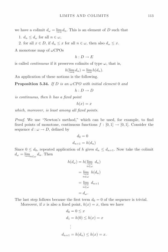
LIMITS AND COLIMITS 113
we have a colimit dω = lim−→ dn. This is an element of D such that
1. dn ≤ dω for all n ∈ ω,2. for all x ∈ D, if dn ≤ x for all n ∈ ω, then also dω ≤ x.
A monotone map of ωCPOs
h : D → E
is called continuous if it preserves colimits of type ω, that is,
h(lim−→ dn) = lim−→h(dn).
An application of these notions is the following.
Proposition 5.34. If D is an ωCPO with initial element 0 and
h : D → D
is continuous, then h has a fixed point
h(x) = x
which, moreover, is least among all fixed points.
Proof. We use “Newton’s method,” which can be used, for example, to findfixed points of monotone, continuous functions f : [0, 1] → [0, 1]. Consider thesequence d : ω → D, defined by
d0 = 0
dn+1 = h(dn)
Since 0 ≤ d0, repeated application of h gives dn ≤ dn+1. Now take the colimitdω = lim−→n∈ω
dn. Then
h(dω) = h(lim−→n∈ω
dn)
= lim−→n∈ω
h(dn)
= lim−→n∈ω
dn+1
= dω.
The last step follows because the first term d0 = 0 of the sequence is trivial.Moreover, if x is also a fixed point, h(x) = x, then we have
d0 = 0 ≤ x
d1 = h(0) ≤ h(x) = x
...
dn+1 = h(dn) ≤ h(x) = x.

114 CATEGORY THEORY
So also dω ≤ x, since dω is the colimit.
Finally, here is an example of how (co)limits depend on the ambient category.We consider colimits of posets and ωCPOs, rather than in them.
Let us define the finite ωCPOs
ωn = {k ≤ n | k ∈ ω}
then we have continuous inclusion maps:
ω0 → ω1 → ω2 → · · ·
In Pos, the colimit exists, and is ω, as can be easily checked. But ω itself isnot ω-complete. Indeed, the sequence
0 ≤ 1 ≤ 2 ≤ · · ·
has no colimit. Therefore, the colimit of the ωn in the category of ωCPOs, if itexists, must be something else. In fact, it is ω + 1.
0 ≤ 1 ≤ 2 ≤ · · · ≤ ω
For then any bounded sequence has a colimit in the bounded part, and anyunbounded one has ω as colimit. The moral is that even ω-colimits are not alwayscreated in Sets, and indeed the colimit is sensitive to the ambient category inwhich it is taken.
5.7 Exercises
1. Show that a pullback of arrows
A×X Bp2� B
A
p1
�
f� X
g
�
in a category C is the same thing as their product in the slice categoryC/X.
2. Let C be a category with pullbacks.
(a) Show that an arrow m : M → X in C is monic if and only if thediagram below is a pullback.

LIMITS AND COLIMITS 115
M1M � M
M
1M
�
m� X
m
�
Thus, as an object in C/X, m is monic iff m×m ∼= m.(b) Show that the pullback along an arrow f : Y → X of a pullback square
over X,A×X B � B
A�
� X�
is again a pullback square over Y . (Hint: draw a cube and use the two-pullbacks lemma.) Conclude that the pullback functor f∗ preservesproducts.
(c) Conclude from the foregoing that in a pullback square
M ′ � M
A′
m′
�
f� A
m
�
if m is monic, then so is m′.
3. Show directly that in any category, given a pullback square
M ′ � M
A′
m′
�
f� A
m
�
if m is monic, then so is m′.4. For any object A in a category C and any subobjects M,N ∈ SubC(A),
show M ⊆ N iff for every generalized element z : Z → A (arbitrary arrowwith codomain A):
z ∈A M implies z ∈A N.

116 CATEGORY THEORY
5. For any object A in a category C and any subobjects M,N ∈ SubC(A),show M ⊆ N iff for every generalized element z : Z → A (arbitrary arrowwith codomain A):
z ∈A M implies z ∈A N.
6. (Equalizers by pullbacks and products) Show that a category with pull-backs and products has equalizers as follows: given arrows f, g : A → B,take the pullback indicated below, where Δ = 〈1B , 1B〉:
E � B
A
e
�
〈f, g〉� B ×B
Δ
�
Show that e : E → A is the equalizer of f and g.7. Let C be a locally small category with all small limits, and D : J → C
any diagram in C. Show that for any object C ∈ C, the representablefunctor
HomC(C,−) : C → Sets
preserves the limit of D.8. (Partial maps) For any category C with pullbacks, define the category
Par(C) of partial maps in C as follows: the objects are the same as thoseof C, but an arrow f : A → B is a pair (|f |, Uf ), where Uf � A is asubobject and |f | : Uf → B is a suitable equivalence class of arrows, asindicated in the diagram:
Uf|f | � B
A�
�
Composition of (|f |, Uf ) : A → B and (|g|, Ug) : B → C is given by takinga pullback and then composing to get (|g ◦ f |, |f |∗(Ug)), as suggested bythe following diagram:

LIMITS AND COLIMITS 117
|f |∗(Ug) � Ug |g|� C
Uf
�
�
|f |� B
�
�
A�
�
Verify that this really does define a category, and show that there is afunctor,
C → Par(C)
which is the identity on objects.9. Suppose the category C has limits of type J, for some index category J.
For diagrams F and G of type J in C, a morphism of diagrams θ : F → Gconsists of arrows θi : Fi → Gi for each i ∈ J such that for each α :i → j in J, one has θjF (α) = G(α)θi (a commutative square). This makesDiagrams(J,C) into a category (check this).Show that taking the vertex-objects of limiting cones determines a functor:
lim←−J
: Diagrams(J,C) → C
Infer that for any set I, there is a product functor,∏i∈I
: SetsI → Sets
for I-indexed families of sets (Ai)i∈I .10. (Pushouts)
(a) Dualize the definition of a pullback to define the “copullback” (usuallycalled the “pushout”) of two arrows with common domain.
(b) Indicate how to construct pushouts using coproducts and coequalizers(proof “by duality”).
11. Let R ⊆ X × X be an equivalence relation on a set X, with quotientq : X � Q. Show that the following is an equalizer:
PQPq � PX
Pr1�
Pr2
� PR,
where r1, r2 : R ⇒ X are the two projections of R ⊆ X, and P is the(contravariant) powerset functor. (Hint: PX ∼= 2X .)
118 CATEGORY THEORY
12. Consider the sequence of posets [0] → [1] → [2] → . . . , where
[n] = {0 ≤ · · · ≤ n},
and the arrows [n] → [n + 1] are the evident inclusions. Determine thelimit and colimit posets of this sequence.
13. Consider sequences of monoids,
M0 → M1 → M2 → . . .
N0 ← N1 ← N2 ← . . .
and the following limits and colimits, constructed in the category ofmonoids:
lim−→n
Mn, lim←−n
Mn, lim−→n
Nn, lim←−n
Nn.
(a) Suppose all Mn and Nn are abelian groups. Determine whether eachof the four (co)limits lim−→n
Mn etc. is also an abelian group.
(b) Suppose all Mn and Nn are finite groups. Determine whether each ofthe four (co)limits lim−→n
Mn etc. has the following property: for everyelement x, there is a number k such that xk = 1 (the least such k iscalled the order of x).

6
EXPONENTIALS
We have now managed to unify most of the universal mapping properties thatwe have seen so far with the notion of limits (or colimits). Of course, the freealgebras are an exception to this. In fact, it turns out that there is a commonsource of such universal mapping properties, but it lies somewhat deeper, inthe notion of adjoints, which unify free algebras, limits, and other universals ofvarious kinds.
Next we are going to look at one more elementary universal structure, whichis also an example of a universal that is not a limit. This important structureis called an “exponential,” and it can be thought of as a categorical notionof a “function space.” As we shall see it subsumes much more than just that,however.
6.1 Exponential in a category
Let us start by considering a function of sets,
f(x, y) : A×B → C
written using variables x over A and y over B. If we now hold a ∈ A fixed, wehave a function
f(a, y) : B → C
and thus an element
f(a, y) ∈ CB
of the set of all such functions.Letting a vary over A then gives a map, which I write like this
f : A → CB
defined by a �→ f(a, y).The map f : A → CB takes the “parameter” a to the function f(a, y) :
B → C. It is uniquely determined by the equation
f(a)(b) = f(a, b).

120 CATEGORY THEORY
Indeed, any map
φ : A → CB
is uniquely of the form
φ = f
for some f : A×B → C. For we can set
f(a, b) := φ(a)(b).
What this means, in sum, is that we have an isomorphism of Hom-sets:
HomSets(A×B,C) ∼= HomSets(A,CB)
That is, there is a bijective correspondence between functions of the formf : A × B → C and those of the form f : A → CB , which we can displayschematically thus
f : A×B → C
f : A → CB
This bijection is mediated by a certain operation of evaluation, which we haveindicated in the foregoing by using variables. In order to generalize the indica-ted bijection to other categories, we are going to need to make this evaluationoperation explicit, too.
In Sets, it is the function
eval : CB ×B → C
defined by (g, b) �→ g(b), that is,
eval(g, b) = g(b).
This evaluation function has the following UMP: given any set A and anyfunction
f : A×B → C
there is a unique function
f : A → CB
such that eval ◦ (f × 1B) = f . That is,
eval(f(a), b) = f(a, b). (6.1)
Here is the diagram:
CB CB ×Beval� C
A
f
�
A×B
f × 1B
�
f
�

EXPONENTIALS 121
You can read the equation (6.1) off from this diagram by taking a pair ofelements (a, b) ∈ A×B and chasing them around both ways, using the fact that(f × 1B)(a, b) = (f(a), b).
Now, the property just stated of the set CB and the evaluation functioneval : CB × B → C is one that makes sense in any category having binaryproducts. It says that evaluation is “the universal map into C from a productwith B.” Precisely, we have the following:
Definition 6.1. Let the category C have binary products. An exponential ofobjects B and C consists of an object
CB
and an arrow
ε : CB ×B → C
such that, for any object A and arrow
f : A×B → C
there is a unique arrow
f : A → CB
such that
ε ◦ (f × 1B) = f
all as in the diagram
CB CB ×Bε � C
A
f
�
A×B
f × 1B
�
f
�
Here is some terminology:
• ε : CB ×B → C is called evaluation.
• f : A → CB is called the (exponential) transpose of f .
• Given any arrow
g : A → CB
we write
g := ε ◦ (g × 1B) : A×B → C

122 CATEGORY THEORY
and also call g the transpose of g. By the uniqueness clause of the definition,we then have
˜g = g
and for any f : A×B → C,
¯f = f.
Briefly, transposition of transposition is the identity.
Thus in sum, the transposition operation
(f : A×B → C) �−→ (f : A → CB)
provides an inverse to the induced operation
(g : A → CB) �−→ (g = ε ◦ (g × 1B) : A×B → C),
yielding the desired isomorphism,
HomC(A×B,C) ∼= HomC(A,CB).
6.2 Cartesian closed categories
Definition 6.2. A category is called cartesian closed, if it has all finite productsand exponentials.
Example 6.3. We already have Sets as one example, but note that also Setsfin
is cartesian closed, since for finite sets M,N , the set of functions NM hascardinality
|NM | = |N ||M |
and so is also finite.
Example 6.4. Recall that the category Pos of posets has as arrows f : P → Qthe monotone functions, p ≤ p′ implies fp ≤ fp′. Given posets P and Q, theposet P ×Q has pairs (p, q) as elements, and is partially ordered by
(p, q) ≤ (p′, q′) iff p ≤ p′ and q ≤ q′.
Thus, the evident projections
P �π1
P ×Qπ2
� Q
are monotone, as is the pairing
〈f, g〉 : X → P ×Q
if f : X → P and g : X → Q are monotone.

EXPONENTIALS 123
For the exponential QP , we take the set of monotone functions,
QP = {f : P → Q | f monotone }
ordered pointwise, that is,
f ≤ g iff fp ≤ gp for all p ∈ P .
The evaluation
ε : QP × P → Q
and transposition
f : X → QP
of a given arrow
f : X × P → Q
are the usual ones of the underlying functions. Thus, we need only show thatthese are monotone.
To that end, given (f, p) ≤ (f ′, p′) in QP × P , we have
ε(f, p) = f(p)
≤ f(p′)
≤ f ′(p′)
= ε(f ′, p′)
so ε is monotone. Now take f : X × P → Q monotone and let x ≤ x′. We needto show
f(x) ≤ f(x′) in QP
which means
f(x)(p) ≤ f(x′)(p) for all p ∈ P .
But f(x)(p) = f(x, p) ≤ f(x′, p) = f(x′)(p).
Example 6.5. Now let us consider what happens if we restrict to the categoryof ωCPOs (see example 5.33). Given two ωCPOs P and Q, we take as anexponential the subset,
QP = {f : P → Q | f monotone and ω-continuous}.
Then take evaluation ε : QP ×P → Q and transposition as before, for functions.Then, since we know that the required equations are satisfied, we just need tocheck the following:
• QP is an ωCPO

124 CATEGORY THEORY
• ε is ω-continuous
• f is ω-continuous if f is so
We leave this as an exercise!
Example 6.6. An example of a somewhat different sort is provided by the cate-gory Graphs of graphs and their homomorphisms. Recall that a graph G consistsof a pair of sets Ge and Gv—the edges and vertices—and a pair of functions,
Ge
Gv
sG
�
tG
�
called the source and target maps. A homomorphism of graphs h : G → His a mapping of edges to edges and vertices to vertices, preserving sources andtargets, that is, is a pair of maps hv : Gv → Hv and he : Ge → He, making thetwo obvious squares commute.
Gehe � He
Gv
sG
�
tG
� hv � He
sH
�
tH
�
The product G×H of two graphs G and H, like the product of categories, hasas vertices the pairs (g, h) of vertices g ∈ G and h ∈ H, and similarly the edgesare pairs of edges (u, v) with u an edge in G and v and edge in H. The sourceand target operations are, then, “pointwise”: s(u, v) = (s(u), s(v)), etc.
Ge ×He
Gv ×Hv
sG × sH
�
tG × tH
�
Now, the exponential graph HG has as vertices the (arbitrary!) maps ofvertices ϕ : Gv → Hv. An edge θ from ϕ to another vertex ψ : Gv → Hv is afamily of edges (θe) in H, one for each edge e ∈ G, such that s(θe) = ϕ(s(e)) andt(θe) = ψ(t(e)). In other words, θ is a map θ : Ge → He making the following

EXPONENTIALS 125
commute:
Gv� s
Get � Gv
Hv
ϕ
��
sHe
θ
�
t� Hv
ψ
�
Imagining G as a certain configuration of edges and vertices, and the maps ϕand ψ as two different “pictures” or “images” of the vertices of G in H, the edgeθ : ϕ → ψ appears as a family of edges in H, labeled by the edges of G, eachconnecting the source vertex in ϕ to the corresponding target one in ψ. (Thereader should draw a diagram at this point.) The evaluation homomorphismε : HG × G → H takes a vertex (ϕ, g) to the vertex ϕ(g), and an edge (θ, e)to the edge θe. The transpose of a graph homomorphism f : F × G → H isthe homomorphism f : F → HG taking a vertex a ∈ F to the mapping onvertices f(a,−) : Gv → Hv, and an edge c : a → b in F to the mapping of edgesf(c,−) : Ge → He.
We leave the verification of this cartesian closed structure as an exercise forthe reader.
Next, we derive some of the basic facts about exponentials and cartesianclosed categories. First, let us ask, what is the transpose of evaluation?
ε : BA ×A → B
It must be an arrow ε : BA → BA such that
ε(ε× 1A) = ε
that is, making the following diagram commute:
BA ×Aε � B
BA ×A
ε× 1A
�
ε
�
Since 1BA × 1A = 1(BA×A) clearly has this property, we must have
ε = 1BA
and so we also know that ε = (1BA).Now let us show that the operation X �→ XA on a CCC is functorial.

126 CATEGORY THEORY
Proposition 6.7. In any cartesian closed category C, exponentiation by a fixedobject A is a functor,
(−)A : C → C.
Toward the proof, consider first the case of sets. Given some function
β : B → C,
we put
βA : BA → CA
defined by
f �→ β ◦ f.
That is,
A
B
f
�
β� C
β ◦ f = βA(f)
�
This assignment is functorial, because for any α : C → D
(α ◦ β)A(f) = α ◦ β ◦ f
= α ◦ βA(f)
= αA ◦ βA(f).
Whence (α ◦ β)A = αA ◦ βA. Also,
(1B)A(f) = 1B ◦ f
= f
= 1BA(f).
So (1B)A = 1BA . Thus, (−)A is indeed a functor; of course, it is just therepresentable functor Hom(A,−) that we have already considered.
In a general CCC then, given β : B → C, we define
βA : BA → CA
by
βA := (β ◦ ε).

EXPONENTIALS 127
That is, we take the transpose of the composite
BA ×Aε→ B
β→ C
giving
βA : BA → CA.
It is easier to see in the form
CA CA ×Aε � C
BA
βA
�
BA ×A
βA × 1A
�
ε� B
β
�
Now, clearly,
(1B)A = 1BA : BA → BA
by examining
BA ×Aε � B
BA ×A
1(BA×A) = 1BA × 1A
�
ε� B
1B
�
Quite similarly, given
Bβ→ C
γ→ D
we have
γA ◦ βA = (γ ◦ β)A.
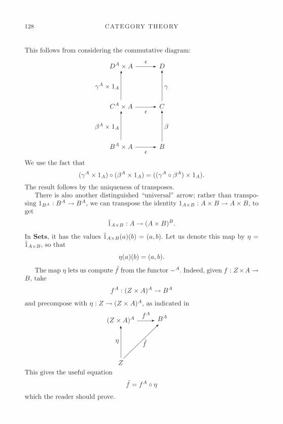
128 CATEGORY THEORY
This follows from considering the commutative diagram:
DA ×Aε � D
CA ×A
γA × 1A
�
ε� C
γ
�
BA ×A
βA × 1A
�
ε� B
β
�
We use the fact that
(γA × 1A) ◦ (βA × 1A) = ((γA ◦ βA)× 1A).
The result follows by the uniqueness of transposes.There is also another distinguished “universal” arrow; rather than transpo-
sing 1BA : BA → BA, we can transpose the identity 1A×B : A×B → A×B, toget
1A×B : A → (A×B)B .
In Sets, it has the values 1A×B(a)(b) = (a, b). Let us denote this map by η =1A×B , so that
η(a)(b) = (a, b).
The map η lets us compute f from the functor −A. Indeed, given f : Z×A →B, take
fA : (Z ×A)A → BA
and precompose with η : Z → (Z ×A)A, as indicated in
(Z ×A)A fA� BA
Z
η
�
f
�
This gives the useful equation
f = fA ◦ η
which the reader should prove.

EXPONENTIALS 129
6.3 Heyting algebras
Any Boolean algebra B, regarded as a poset category, has finite products 1 anda ∧ b. We can also define the exponential in B by
ba = (¬a ∨ b)
which we also write a ⇒ b. The evaluation arrow is
(a ⇒ b) ∧ a ≤ b.
This always holds since
(¬a ∨ b) ∧ a = (¬a ∧ a) ∨ (b ∧ a) = 0 ∨ (b ∧ a) = b ∧ a ≤ b.
To show that a ⇒ b is indeed an exponential in B, we just need to verify that ifa ∧ b ≤ c then a ≤ b ⇒ c, that is, transposition. But if a ∧ b ≤ c, then
¬b ∨ (a ∧ b) ≤ ¬b ∨ c = b ⇒ c.
But we also have
a ≤ ¬b ∨ a ≤ (¬b ∨ a) ∧ (¬b ∨ b) = ¬b ∨ (a ∧ b).
This example suggests generalizing the notion of a Boolean algebra to thatof a cartesian closed poset. Indeed, consider first the following stronger notion.
Definition 6.8. A Heyting algebra is a poset with
1. Finite meets: 1 and p ∧ q,2. Finite joins: 0 and p ∨ q,3. Exponentials: for each a, b, an element a ⇒ b such that
a ∧ b ≤ c iff a ≤ b ⇒ c.
The stated condition on exponentials a ⇒ b is equivalent to the UMP in thecase of posets. Indeed, given the condition, the transpose of a∧b ≤ c is a ≤ b ⇒ cand the evaluation (a ⇒ b)∧a ≤ b follows immediately from a ⇒ b ≤ a ⇒ b (theconverse is just as simple).
First, observe that every Heyting algebra is a distributive lattice, that is, forany a, b, c, one has
(a ∨ b) ∧ c = (a ∧ c) ∨ (b ∧ c).
Indeed, we have
(a ∨ b) ∧ c ≤ z iff a ∨ b ≤ c ⇒ z
iff a ≤ c ⇒ z and b ≤ c ⇒ z
iff a ∧ c ≤ z and b ∧ c ≤ z
iff (a ∧ c) ∨ (b ∧ c) ≤ z.

130 CATEGORY THEORY
Now pick z = (a∨b)∧c and read the equivalences downward to get one direction,then do the same with z = (a∧ c)∨ (b∧ c) and reading the equivalences upwardto get the other direction.
Remark 6.9. The foregoing distributivity is actually a special case of the moregeneral fact that in a cartesian closed category with coproducts, the productsnecessarily distribute over the coproducts,
(A + B)× C ∼= (A× C) + (B × C).
Although we could prove this now directly, a much more elegant proof (generali-zing the one above for the poset case) will be available to us once we have accessto the Yoneda lemma. For this reason, we defer the proof of distributivity to8.6.
One may well wonder whether all distributive lattices are Heyting algebras.The answer is in general, no; but certain ones always are.
Definition 6.10. A poset is (co) complete if it is so as a category, thus if it hasall set-indexed meets
∧i∈I ai (resp. joins
∨i∈I ai). For posets, completeness and
cocompleteness are equivalent (exercise!). A lattice, Heyting algebra, Booleanalgebra, etc. is called complete if it is so as a poset.
Proposition 6.11. A complete lattice is a Heyting algebra iff it satisfies theinfinite distributive law
a ∧(∨
i
bi
)=
∨i
(a ∧ bi).
Proof. One shows that Heyting algebra implies distributivity just as in the finitecase. To show that the infinite distributive law implies Heyting algebra, set
a ⇒ b =∨
x∧a≤b
x.
Then, if
y ∧ a ≤ b
then y ≤ ∨x∧a≤b x = a ⇒ b. And conversely, if y ≤ a ⇒ b, then y ∧ a ≤
(∨
x∧a≤b x) ∧ a =∨
x∧a≤b(x ∧ a) ≤ ∨b = b.
Example 6.12. For any set A, the powerset P (A) is a complete Heyting algebrawith unions and intersections as joins and meets, since it satisfies the infinitedistributive law. More generally, the lattice of open sets of a topological space isalso a Heyting algebra, since the open sets are closed under finite intersectionsand arbitrary unions.

EXPONENTIALS 131
Of course, every Boolean algebra is a Heyting algebra with a ⇒ b = ¬a ∨ b, aswe already showed. But in general, a Heyting algebra is not Boolean. Indeed, wecan define a proposed negation by
¬a = a ⇒ 0
as must be the case, since in a Boolean algebra ¬a = ¬a ∨ 0 = a ⇒ 0. Thena ≤ ¬¬a since a ∧ (a ⇒ 0) ≤ 0. But, conversely, ¬¬a ≤ a need not hold in aHeyting algebra. Indeed, in a topological space X, the negation ¬U of an opensubset U is the interior of the complement X − U . Thus, for example, in thereal interval [0, 1], we have ¬¬(0, 1) = [0, 1].
Moreover, the law,1 ≤ a ∨ ¬a
also need not hold in general. In fact, the concept of a Heyting algebra is thealgebraic equivalent of the intuitionistic propositional calculus, in the same sensethat Boolean algebras are an algebraic formulation of the classical propositionalcalculus.
6.4 Propositional calculus
In order to make the connection between Heyting algebras and propositionalcalculus more rigorous, let us first give a specific system of rules for the intui-tionistic propositional calculus (IPC). This we do in terms of entailments p qbetween formulas p and q:
1. is reflexive and transitive2. p �3. ⊥ p
4. p q and p r iff p q ∧ r
5. p r and q r iff p ∨ q r
6. p ∧ q r iff p q ⇒ r
This is a complete system for IPC, equivalent to the more standard presenta-tions the reader may have seen. To compare with one perhaps more familiarpresentation, note first that we have an “evaluation” entailment by reflexivityand (6):
p ⇒ q p ⇒ q
(p ⇒ q) ∧ p q
We therefore have the rule of “modus ponens” by (4) and transitivity:
� p ⇒ q and � p
� (p ⇒ q) ∧ p
� q

132 CATEGORY THEORY
Moreover, by (4) there are “projections”:
p ∧ q p ∧ q
p ∧ q p (resp. q)
from which it follows that p ! � ∧ p. Thus, we get one of the usual axioms forproducts:
p ∧ q p
� ∧ (p ∧ q) p
� (p ∧ q) ⇒ p
Now let us derive the usual axioms for ⇒, namely,
1. p ⇒ p,2. p ⇒ (q ⇒ p),3. (p ⇒ (q ⇒ r)) ⇒ ((p ⇒ q) ⇒ (p ⇒ r)).
The first two are almost immediate:
p p
� ∧ p p
� p ⇒ p
p ∧ q p
p q ⇒ p
� ∧ p (q ⇒ p)
� p ⇒ (q ⇒ p)
For the third one, we use the fact that ⇒ distributes over ∧ on the right:
a ⇒ (b ∧ c) ! (a ⇒ b) ∧ (a ⇒ c)
This is a special case of the exercise:
(B × C)A ∼= BA × CA
We also use the following simple fact, which will be recognized as a special caseof proposition 6.7:
a b implies p ⇒ a p ⇒ b (6.2)

EXPONENTIALS 133
Then we have
(q ⇒ r) ∧ q r
p ⇒ ((q ⇒ r) ∧ q) p ⇒ r
(p ⇒ (q ⇒ r)) ∧ (p ⇒ q) p ⇒ r by (6.3)
(p ⇒ (q ⇒ r)) (p ⇒ q) ⇒ (p ⇒ r)
� (p ⇒ (q ⇒ r)) ⇒ ((p ⇒ q) ∧ (p ⇒ r)).
The “positive” fragment of IPC, involving only the logical operations
�, ∧, ⇒corresponds to the notion of a cartesian closed poset. We then add ⊥ and dis-junction p∨q on the logical side and finite joins on the algebraic side to arrive ata correspondence between IPC and Heyting algebras. The exact correspondenceis given by mutually inverse constructions between Heyting algebras and IPCs.We briefly indicate one direction of this correspondence, leaving the other oneto the reader’s ingenuity.
Given any IPSs L, consisting of propositional formulas p, q, r, . . . over someset of variables x, y, z, . . . together with the rules of inference stated above, andperhaps some distinguished formulas a, b, c, . . . as axioms, one constructs from La Heyting algebra HA(L), called the Lindenbaum–Tarski algebra, consisting ofequivalence classes [p] of formulas p, where
[p] = [q] iff p ! q (6.3)
The ordering in HA(L) is given by
[p] ≤ [q] iff p q (6.4)
This is clearly well defined on equivalence classes, in the sense that if p q and[p] = [p′] then p′ q, and similarly for q. The operations in HA(L) are theninduced in the expected way by the logical operations:
1 = [�]
0 = [⊥]
[p] ∧ [q] = [p ∧ q]
[p] ∨ [q] = [p ∨ q]
[p] ⇒ [q] = [p ⇒ q]
Again, these operations are easily seen to be well defined on equivalence classes,and they satisfy the laws for a Heyting algebra because the logical rules evidentlyimply them.
Lemma 6.13. Observe that, by (6.3), the Heyting algebra HA(L) has theproperty that a formula p is provable � p if and only if [p] = 1.

134 CATEGORY THEORY
Now define an interpretation M of L in a Heyting algebra H to be an assi-gnment of the basic propositional variables x, y, z, . . . to elements of H, whichwe shall write as [[x]], [[y]], [[z]], .... An interpretation then extends to all formulasby recursion in the evident way, that is, [[p ∧ q]] = [[p]]∧ [[q]], etc. An interpretationis called a model of L if for every theorem � p, one has [[p]] = 1. Observe thatthere is a canonical interpretation of L in HA(L) given by [[x]] = [x]. One showseasily by induction that, for any formula p, moreover, [[p]] = [p]. Now lemma 6.13tells us that this interpretation is in fact a model of L and that, moreover, it is“generic,” in the sense that it validates only the provable formulas. We thereforehave the following logical completeness theorem for IPC.
Proposition 6.14. The intuitionistic propositional calculus is complete withrespect to models in Heyting algebras.
Proof. Suppose a formula p is true in all models in all Heyting algebras. Thenin particular, it is so in HA(L). Thus, 1 = [[p]] = [p] in HA(L), and so � p.
In sum, then, a particular instance L of IPC can be regarded as a way ofspecifying (and reasoning about) a particular Heyting algebra HA(L). Indeed, itis essentially a presentation by generators and relations, in just the way that wehave already seen for other algebraic objects like monoids. The Heyting algebraHA(L) even has a UMP with respect to L that is entirely analogous to the UMPof a finitely presented monoid given by generators and relations. Specifically, if,for instance, L is generated by the two elements x, y subject to the single “axiom”x ∨ y ⇒ x ∧ y, then in HA(L) the elements [x] and [y] satisfy [x] ∨ [y] ≤ [x] ∧ [y](which is of course equivalent to ([x]∨[y] ⇒ [x]∧[y]) = 1), and given any Heytingalgebra A with two elements a and b satisfying a ∨ b ≤ a ∧ b, there is a uniqueHeyting homomorphism h : HA(L) → A with h([x]) = a and h([y]) = b. In thissense, the Lindenbaum–Tarski Heyting algebra HA(L), being finitely presentedby the generators and axioms of L, can be said to contain a “universal model”of the theory determined by L.
6.5 Equational definition of CCC
The following description of CCCs in terms of operations and equations on acategory is often useful. The proof is entirely routine and left to the reader.
Proposition 6.15. A category C is a CCC iff it has the following structure:
• A distinguished object 1, and for each object C there is given an arrow
!C : C → 1
such that for each arrow f : C → 1,
f =!C .

EXPONENTIALS 135
• For each pair of objects A,B, there is given an object A×B and arrows,
p1 : A×B → A and p2 : A×B → B
and for each pair of arrows f : Z → A and g : Z → B, there is given anarrow,
〈f, g〉 : Z → A×B
such that
p1〈f, g〉 = f
p2〈f, g〉 = g
〈p1h, p2h〉 = h for all h : Z → A×B.
• For each pair of objects A,B, there is given an object BA and an arrow,
ε : BA ×A → B
and for each arrow f : Z ×A → B, there is given an arrow
f : Z → BA
such that
ε ◦ (f × 1A) = f
and
˜(ε ◦ (g × 1A)) = g
for all g : Z → BA. Here, and generally, for any a : X → A and b : Y → B,we write
a× b = 〈a ◦ p1, b ◦ p2〉 : X × Y → A×B.
It is sometimes easier to check these equational conditions than to verify thecorresponding UMPs. Section 6.6 provides an example of this sort.
6.6 λ-calculus
We have seen that the notions of a cartesian closed poset with finite joins (i.e.,a Heyting algebra) and intuitionistic propositional calculus are essentially thesame:
HA ∼ IPC.
These are two different ways of describing one and the same structure; whereby,to be sure, the logical description contains some superfluous data in the choiceof a particular presentation.
We now want to consider another, very similar, correspondence betweensystems of logic and categories, involving more general CCCs. Indeed, the fore-

136 CATEGORY THEORY
going correspondence was the poset case of the following general one betweenCCCs and λ-calculus:
CCC ∼ λ-calculus.
These notions are also essentially equivalent, in a sense that we now sketch (amore detailed treatment can be found in the book by Lambek and Scott). Theyare two different ways of representing the same idea, namely that of a collectionof objects and functions, with operations of pairing, projection, application, andtransposition (or “currying”).
First, recall the notion of a (typed) λ-calculus from Chapter 2. It consistsof
• Types: A×B, A → B, . . . (and some basic types)
• Terms: x, y, z, . . . : A (variables for each type A)a : A, b : B, . . . (possibly some typed constants)
〈a, b〉 : A×B (a : A, b : B)
fst(c) : A (c : A×B)
snd(c) : B (c : A×B)
ca : B (c : A → B, a : A)
λx.b : A → B (x : A, b : B)
• Equations, including at least all instances of the following:
fst(〈a, b〉) = a
snd(〈a, b〉) = b
〈fst(c), snd(c)〉 = c
(λx.b)a = b[a/x]
λx.cx = c (no x in c)
Given a particular such λ-calculus L, the associated category of types C(L)was then defined as follows:
• Objects: the types,
• Arrows A → B: equivalence classes of closed terms [c] : A → B, identifiedaccording to (renaming of bound variables and),
[a] = [b] iff L a = b (6.5)
• Identities: 1A = [λx.x] (where x : A),
• Composition: [c] ◦ [b] = [λx.c(bx)].
We have already seen that this is a well-defined category, and that it hasbinary products. It is a simple matter to add a terminal object. Now let us use

EXPONENTIALS 137
the equational characterization of CCCs to show that it is cartesian closed. Givenany objects A,B, we set BA = A → B, and as the evaluation arrow, we take(the equivalence class of),
ε = λz.fst(z)snd(z) : BA ×A → B (z : Z).
Then for any arrow f : Z ×A → B, we take as the transpose,
f = λzλx.f〈z, x〉 : Z → BA (z : Z, x : A).
It is now a straightforward λ-calculus calculation to verify the two requiredequations, namely,
ε ◦ (f × 1A) = f,
˜(ε ◦ (g × 1A)) = g.
In detail, for the first one recall that
α× β = λw.〈αfst(w), βsnd(w)〉.
So, we have
ε ◦ (f × 1A) = (λz.fst(z)snd(z)) ◦ [(λyλx.f〈y, x〉)× λu.u]
= λv.(λz.fst(z)snd(z))[(λyλx.f〈y, x〉)× λu.u]v
= λv.(λz.fst(z)snd(z))[λw.〈(λyλx.f〈y, x〉)fst(w), (λu.u)snd(w)〉]v= λv.(λz.fst(z)snd(z))[λw.〈(λx.f〈fst(w), x〉), snd(w)〉]v= λv.(λz.fst(z)snd(z))[〈(λx.f〈fst(v), x〉), snd(v)〉]= λv.(λx.f〈fst(v), x〉)snd(v)
= λv.f〈fst(v), snd(v)〉= λv.fv
= f.
The second equation is proved similarly.Let us call a set of basic types and terms, together with a set of equations
between terms, a theory in the λ-calculus. Given such a theory L, the cartesianclosed category C(L) built from the λ-calculus over L is the CCC presented bythe generators and relations stated by L. Just as in the poset case of IPC andHeyting algebras, there is a logical completeness theorem that follows from thisfact. To state it, we require the notion of a model of a theory L in the λ-calculusin an arbitrary cartesian closed category C. We give only a brief sketch to givethe reader the general idea.

138 CATEGORY THEORY
Definition 6.16. A model of L in C is an assignment of the types and termsof L to objects and arrows of C:
X basic type � [[X]] object
b : A → B basic term � [[b]] : [[A]] → [[B]] arrow
This assignment is then extended to all types and terms in such a way that theλ-calculus operations are taken to the corresponding CCC ones:
[[A×B]] = [[A]]× [[B]]
[[〈f, g〉]] = 〈[[f ]], [[g]]〉etc.
Finally, it is required that all the equations of L are satisfied, in the sense that
L [a] = [b] : A → B implies [[a]] = [[b]] : [[A]] → [[B]]. (6.6)
This is what is sometimes called “denotational semantics” for the λ-calculus.It is essentially the conventional, set-theoretic semantics for first-order logic, butextended to higher types, restricted to equational theories, and generalized toCCCs.
For example, let L be the theory with one basic type X, two basic terms,
u : X
m : X ×X → X
and the usual equations for associativity and units,
m〈u, x〉 = x
m〈x, u〉 = x
m〈x,m〈y, z〉〉 = m〈m〈x, y〉, z〉.Thus, L is just the usual equational theory of monoids. Then a model of L ina cartesian closed category C is nothing but a monoid in C, that is, an objectM = [[X]] equipped with a distinguished point
[[u]] : 1 → M
and a binary operation
[[m]] : M ×M → M
satisfying the unit and associativity laws.Note that by (6.5) and (6.6), there is a model of L in C(L) with the
property that [[a]] = [[b]] : X → Y if and only if a = b is provable inL. In this way, one can prove the following CCC completeness theorem forλ-calculus.

EXPONENTIALS 139
Proposition 6.17. For any theory L in the λ-calculus, one has the following:
1. For any terms a, b, L a = b iff for all models M in CCCs, [[a]]M = [[b]]M .2. Moreover, for any type A, there is a closed t : A iff for all models M in
CCCs, there is an arrow 1 → [[A]]M .
This proposition says that the λ-calculus is deductively sound and completefor models in CCCs. It is worth emphasizing that completeness is not true if onerestricts attention to models in the single category Sets; indeed, there are manyexamples of theories in λ-calculus in which equations holding for all models inSets are still not provable (see the exercises for an example).
Soundness (i.e., the “only if” direction of the above statements) follows fromthe following UMP of the cartesian closed category C(L), analogous to the onefor any algebra presented by generators and relations. Given any model M of Lin any cartesian closed category C, there is a unique functor,
[[−]]M : C(L) → C
preserving the CCC structure, given by
[[X]]M = M
for the basic type X, and similarly for the other basic types and terms of L. Inthis precise sense, the theory L is a presentation of the cartesian closed categoryC(L) by generators and relations.
Finally, let us note that the notions of λ-calculus and CCC are essentially“equivalent,” in the sense that any cartesian closed category C also gives riseto a λ-calculus L(C), and this construction is essentially inverse to the one justsketched.
Briefly, given C, we define L(C) by
• Basic types: the objects of C
• Basic terms: a : A → B for each a : A → B in C
• Equations: many equations identifying the λ-calculus operations with thecorresponding category and CCC structure on C, for example,
λx.fst(x) = p1
λx.snd(x) = p2
λy.f(x, y) = f(x)
g(f(x)) = (g ◦ f)(x)
λy.y = 1A
This suffices to ensure that there is an isomorphism of categories,
C(L(C)) ∼= C.

140 CATEGORY THEORY
Moreover, the theories L and L(C(L)) are also “equivalent” in a suitable sense,involving the kinds of considerations typical of comparing different presenta-tions of algebras. We refer the reader to the excellent book by Lambek and Scott(1986), for further details.
6.7 Variable sets
We conclude with a special kind of CCC related to the so-called Kripke modelsof logic, namely categories of variable sets. These categories provide specificexamples of the “algebraic” semantics of IPC and λ-calculus just given.
6.7.1 IPC
Let us begin by very briefly reviewing the notion of a Kripke model of IPC fromour algebraic point of view; we focus on the positive fragment involving only�, p ∧ q, p ⇒ q, and variables.
A Kripke model of this language L consists of a poset I of “possibleworlds,” which we write i ≤ j, together with a relation between worlds i andpropositions p,
i � p,
read “p holds at i.” This relation is assumed to satisfy the following conditions:
(1) i � p and i ≤ j implies j � p
(2) i � �(3) i � p ∧ q iff i � p and i � q
(4) i � p ⇒ q iff j � p implies j � q for all j ≥ i.
One then setsI � p iff i � p for all i ∈ I.
And finally, we have the well-known theorem,
Theorem 6.18 (Kripke completeness for IPC). A propositional formula pis provable from the rules for IPC iff it holds in all Kripke models, that is, iffI � p for all relations � over all posets I,
IPC p iff I � p for all I.
Now let us see how to relate this result to our formulation of the semantics ofIPC in Heyting algebras. First, the relation � ⊆ I × Prop(L) between worlds Iand propositional formulas Prop(L) can be equivalently formulated as a mapping,
[[−]] : Prop(L) −→ 2I , (6.7)
where we write 2I = HomPos(I,2) for the exponential poset of monotone mapsfrom I into the poset 2 = {⊥ ≤ �}. This poset is a CCC, and indeed a Heyting

EXPONENTIALS 141
algebra, the proof of which we leave as an exercise for the reader. The mapping(6.7) is determined by the condition
[[p]](i) = � iff i � p.
Now, in terms of the Heyting algebra semantics of IPC developed in Section6.4 (adapted in the evident way to the current setting without the coproducts⊥, p ∨ q, and writing HA− for Heyting algebras without coproducts, i.e., posetCCCs), the poset HA−(L) is a quotient of Prop(L) by the equivalence relationof mutual derivability p ! q, which clearly makes it a CCC, and the map (6.7)therefore determines a model (with the same name),
[[−]] : HA−(L) −→ 2I .
Indeed, condition (1) above ensures that [[p]] : I → 2 is monotone, and (2)–(4) ensure that [[−]] is a homomorphism of poset CCCs, that is, that it ismonotone and preserves the CCC structure (exercise!). Thus, a Kripke modelis just an “algebraic” model in a Heyting algebra of the special form 2I . TheKripke completeness theorem for positive IPC above then follows from Heyting-valued completeness theorem proposition 6.14 together with the following, purelyalgebraic, embedding theorem for poset CCCs.
Proposition 6.19. For every poset CCC A, there is a poset I and an injective,monotone map,
y : A � 2I ,
preserving CCC structure.
Proof. We can take I = Aop and y(a) : Aop → 2, the “truth-value” of x ≤ a,that is, y(a) is determined by
y(a)(x) = � iff x ≤ a.
Clearly, y(a) is monotone and contravariant, while y itself is monotone and cova-riant. We leave it as an exercise to verify that y is injective and preserves theCCC structure, but note that 2Aop
can be identified with the collection of lowersets S ⊆ A in A, that is, subsets that are closed downward: x ≤ y ∈ S impliesx ∈ S. Under this identification, we then have y(a) = ↓(a) = {x |x ≤ a}.
A proof is also given in Chapter 8 as a consequence of the Yoneda lemma.
The result can be extended from poset CCCs to Heyting algebras, thus reco-vering the usual Kripke completeness theorem for full IPC, by the same argumentusing a more delicate embedding theorem that also preserves the coproducts ⊥and p ∨ q.
6.7.2 λ-calculus
We now want to generalize the foregoing from propositional logic to the λ-calculus, motivated by the insight that the latter is the proof theory of the

142 CATEGORY THEORY
former (according to the Curry–Howard–correspondence). Categorically spea-king, we are generalizing from the poset case to the general case of a CCC.According to the “propositions-as-types” conception behind the C–H correspon-dence, we therefore should replace the poset CCC of idealized propositions 2 withthe general CCC of idealized types Sets. We therefore model the λ-calculus incategories of the form SetsI for posets I, which can be regarded as comprisedof “I-indexed,” or “variable sets,” as we now indicate.
Given a poset I, an I-indexed set is a family of sets (Ai)i∈I together withtransition functions αij : Ai → Aj for each i ≤ j, satisfying the compatibilityconditions:
• αik = αjk ◦ αij whenever i ≤ j ≤ k,
• αii = 1Aifor all i.
In other words, it is simply a functor,
A : I −→ Sets.
We can think of such I-indexed sets as “sets varying in a parameter” from theposet I. For instance, if I = R thought of as time, then an R-indexed set Amay be thought of as a set varying through time: some elements a, b ∈ At maybecome identified over time (the αs need not be injective), and new elementsmay appear over time (the αs need not be surjective), but once an element is inthe set (a ∈ At), it stays in forever (αtt′(a) ∈ At′). For a more general poset I,the variation is parameterized accordingly.
A product of two variable sets A and B can be constructed by taking thepointwise products (A×B)(i) = A(i)×B(i) with the evident transition maps,
αij × βij : A(i)×B(i) → A(j)×B(j) i ≤ j
where βij : Bi → Bj is the transition map for B. This plainly gives an I-indexedset, but to check that it really is a product we need to make SetsI into a categoryand verify the UMP (respectively, the operations and equations of Section 6.5).What is a map of I-indexed sets f : A → B? One natural proposal is this: it isan I-indexed family of functions (fi : Ai → Bi)i∈I that are compatible with thetransition maps, in the sense that whenever i ≤ j, then the following commutes:
Aifi � Bi
Aj
αij
�
fj
� Bj
βij
�
We can think of this condition as saying that f takes elements a ∈ A to elementsf(a) ∈ B without regard to when the transition is made, since given a ∈ Ai it

EXPONENTIALS 143
does not matter if we first wait until j ≥ i and then take fj(αij(a)), or go rightaway to fi(a) and then wait until βij(fi(a)).
Indeed, in Chapter 7 we see that this type of map is exactly what is calleda “natural transformation” of the functors A and B. These maps f : A → Bcompose in the evident way:
(g ◦ f)i = gi ◦ fi : Ai −→ Bi
to make SetsI into a category, the category of I-indexed sets. It is now an easyexercise to confirm that the specification of the product A×B just given reallyis a product in the resulting category SetsI , and the terminal object is obviouslythe constant index set 1, so SetsI has all finite products.
What about exponentials? The first attempt at defining pointwise exponen-tials,
(BA)i = BAii
fails, because the indexing is covariant in B and contravariant in A, as the readershould confirm. The idea that maybe BA is just the collection of all index mapsfrom A to B also fails, because it is not indexed! The solution is a combintion ofthese two ideas which generalizes the “Kripke” exponential as follows. For eachi ∈ I, let
↓(i) ⊆ I
be the lower set below i, regarded as a subposet. Then for any A : I → Sets, letA|i be the restriction,
IA � Sets
↓(i)∪
�
A|i
�
This determines an indexed set over ↓(i). Given any f : A → B and i ∈ I, thereis an evident restriction f |i : A|i → B|i which is defined to be simply (f |i)j = fj
for any j ≤ i. Now we can define
(BA)i = {f : A|i → B|i | f is ↓(i)-indexed}with the transition maps given by
f �→ f |j j ≤ i
It is immediate that this determines an I-indexed set BA. That it is actually theexponential of A and B in SetsI is shown later, as an easy consequence of theYoneda lemma. For the record, we therefore have the following (proof deferred).
Proposition 6.20. For any poset I, the category SetsI of I-indexed sets andfunctions is cartesian closed.

144 CATEGORY THEORY
Definition 6.21. A Kripke model of a theory L in the λ-calculus is a model (inthe sense of definition 6.16) in a cartesian closed category of the form SetsI fora poset I.
For instance, it can be seen that a Kripke model over a poset I of a conventio-nal algebraic theory such as the theory of groups is just an I-indexed group, thatis, a functor I → Group. In particular, if I = O(X)op for a topological space X,then this is just what the topologist calls a “presheaf of groups.” On the otherhand, it also agrees with (or generalizes) the logician’s notion of a Kripke modelof a first-order language, in that it consists of a varying domain of “individuals”equipped with varying structure.
Finally, in order to generalize the Kripke completeness theorem for IPC toλ-calculus, it clearly suffices to sharpen our general CCC completeness theorem,proposition 6.17, to the special models in CCCs of the form SetsI by means ofan embedding theorem analogous to proposition 6.19. Indeed, one can prove thefollowing.
Proposition 6.22. For every CCC C, there is a poset I and a functor,
y : C � SetsI ,
that is injective on both objects and arrows and preserves CCC structure. Moreo-ver, every map between objects in the image of y is itself in the image of y (y is“full”).
The full proof of this result involves methods from topos theory that arebeyond the scope of this book. But a significant part of it, to be given below, isentirely analogous to the proof of the poset case, and will again be a consequenceof the Yoneda lemma.
6.8 Exercises
1. Show that for all finite sets M and N ,
|NM | = |N ||M |,
where |K| is the number of elements in the set K, while NM is the expo-nential in the category of sets (the set of all functions f : M → N), andnm is the usual exponentiation operation of arithmetic.
2. Show that for any three objects A,B,C in a cartesian closed category,there are isomorphisms:
(a) (A×B)C ∼= AC ×BC
(b) (AB)C ∼= AB×C
3. Determine the exponential transpose ε of evaluation ε : BA ×A → B (forany objects in any CCC). In Sets, determine the transpose 1 of the identity

EXPONENTIALS 145
1 : A×B → A×B. Also determine the transpose of ε ◦ τ : A×BA → B,where τ : A×BA → BA ×A is the “twist” arrow τ = 〈p2, p1〉.
4. Is the category of monoids cartesian closed?5. Verify the description given in the text of the exponential graph HG for
two graphs G and H. Determine the exponential 2G, where 2 is the graphv1 → v2 with two vertices and one edge, and G is an arbitrary graph.Determine 2G explicitely for G the graph pictured below.
a � b � c
d
�
6. Consider the category of sets equipped with a (binary) relation, (A,R ⊆A × A), with maps f : (A,R) → (B,S) being those functions f : A → Bsuch that aRa′ implies f(a)Sf(a′). Show this category is cartesian closedby describing it as a subcategory of graphs.
7. Consider the category of sets equipped with a distinguished subset,(A,P ⊆ A), with maps f : (A,P ) → (B,Q) being those functionsf : A → B such that a ∈ P iff f(a) ∈ Q. Show this category is cartesianclosed by describing it as a category of pairs of sets.
8. Consider the category of “pointed sets,” that is, sets equipped with adistinguished element, (A, a ∈ A), with maps f : (A, a) → (B, b) beingthose functions f : A → B such that f(a) = b. Is this category cartesianclosed?
9. Show that for any objects A,B in a cartesian closed category, there is abijective correspondence between points of the exponential 1 → BA andarrows A → B.
10. Show that the category of ωCPOs is cartesian closed, but that the categoryof strict ωCPOs is not (the strict ωCPOs are the ones with initial object⊥, and the continuous maps between them are supposed to preserve ⊥).
11. (a) Show that in any cartesian closed poset with joins p∨ q, the following“distributive” law of IPC holds:
((p ∨ q) ⇒ r) ⇒ ((p ⇒ r) ∧ (q ⇒ r))
(b) Generalize the foregoing problem to an arbitrary category (not neces-sarily a poset), by showing that there is always an arrow of thecorresponding form.
(c) If you are brave, show that the previous two arrows are isomorphisms.
12. Prove that in a CCC C, exponentiation with a fixed base object C is acontravariant functor C(−) : Cop → C, where C(−)(A) = CA.

146 CATEGORY THEORY
13. Show that in a cartesian closed category with coproducts, the productsnecessarily distribute over the coproducts,
(A× C) + (B × C) ∼= (A + B)× C.
14. In the λ-calculus, consider the theory (due to Dana Scott) of a reflexivedomain: there is one basic type D, two constants s and r of types
s : (D → D) → D
r : D → (D → D),
and two equations,
srx = x (x : D)
rsy = y (y : D → D).
Prove that, up to isomorphism, this theory has only one model M in Sets,and that every equation holds in M .
15. Complete the proof from the text of Kripke completeness for the positivefragement of IPC as follows:
(a) Show that for any poset I, the exponential poset 2I is a Heyting alge-bra. (Hint: the limits and colimits are “pointwise,” and the Heytingimplication p ⇒ q is defined at i ∈ I by (p ⇒ q)(i) = � iff for all j ≥i, p(j) ≤ q(j).)
(b) Show that for any poset CCC A, the map y : A → 2Aopdefined in
the text is indeed (i) monotone, (ii) injective, and (iii) preserves CCCstructure.
16. Verify the claim in the text that the products A×B in categories SetsI ofI-indexed sets (I a poset) can be computed “pointwise.” Show, moreover,that the same is true for all limits and colimits.

7
NATURALITY
We now want to start considering categories and functors more systematically,developing the “category theory” of category theory itself, rather than of othermathematical objects, like groups, or formulas in a logical system. Let me empha-size that, while some of this may look a bit like “abstract nonsense,” the ideabehind it is that when one has a particular application at hand, the theorycan then be specialized to that concrete case. The notion of a functor is a casein point; developing its general theory makes it a clarifying, simplifying, andpowerful tool in its many instances.
7.1 Category of categories
We begin by reviewing what we know about the category Cat of categories andfunctors and tying up some loose ends.
We have already seen that Cat has finite coproducts 0, C + D; and finiteproducts 1, C×D. It is very easy to see that there are also all small coproductsand products, constructed analogously. We can therefore show that Cat hasall limits by constructing equalizers. Thus, let categories C and D and parallelfunctors F and G be given, and define the category E and functor E,
EE � C
F �
G� D
as follows (recall that for a category C, we write C0 and C1 for the collectionsof objects and arrows, respectively):
E0 = {C ∈ C0 | F (C) = G(C)}E1 = {f ∈ C1 | F (f) = G(f)}
and let E : E → C be the evident inclusion. This is then an equalizer, as thereader can easily check.
The category E is an example of a subcategory, that is, a monomorphism inCat (recall that equalizers are monic). Often, by a subcategory of a category Cone means specifically a collection U of some of the objects and arrows, U0 ⊆ C0
and U1 ⊆ C1), that is closed under the operations dom, cod, id, and ◦. There is

148 CATEGORY THEORY
then an evident inclusion functor
i : U → C
which is clearly monic.In general, coequalizers of categories are more complicated to describe—
indeed, even for posets, determining the coequalizer of a pair of monotone mapscan be quite involved, as the reader should consider.
There are various properties of functors other than being monic and epic thatturn out to be quite useful in Cat. A few of these are given by the following:
Definition 7.1. A functor F : C → D is said to be
• injective on objects if the object part F0 : C0 → D0 is injective, it issurjective on objects if F0 is surjective.
• Similarly, F is injective (resp. surjective) on arrows if the arrow part F1 :C1 → D1 is injective (resp. surjective).
• F is faithful if for all A,B ∈ C0, the map
FA,B : HomC(A,B) → HomD(FA,FB)
defined by f �→ F (f) is injective.
• Similarly, F is full if FA,B is always surjective.
What is the difference between being faithful and being injective on arrows?Consider, for example, the “codiagonal functor” ∇ : C + C → C, as indicatedin the following:
C � C + C � C
C
∇
�
1C
�
1C�
∇ is faithful, but not injective on arrows.A full subcategory
U � C
consists of some objects of C and all of the arrows between them (thus satisfyingthe closure conditions for a subcategory). For example, the inclusion functorSetsfin � Sets is full and faithful, but the forgetful functor Groups � Setsis faithful but not full.
Example 7.2. There is another “forgetful” functor for groups, namely to thecategory Cat of categories,
G : Groups → Cat.

NATURALITY 149
Observe that this functor is full and faithful, since a functor between groupsF : G(A) → G(B) is exactly the same thing as a group homomorphism.
And exactly the same situation holds for monoids.For posets, too, there is a full and faithful, forgetful functor
P : Pos → Cat
again because a functor between posets F : P (A) → P (B) is exactly amonotone map. And the same thing holds for the “discrete category” functorS : Sets → Cat.
Thus, Cat provides a setting for comparing structures of many different kinds.For instance, one can have a functor R : G → C from a group G to a categoryC that is not a group. If C is a poset, then any such functor must be trivial(why?). But if C is, say, the category of finite dimensional, real vector spacesand linear maps, then a functor R is exactly a linear representation of the groupG, representing every element of G as an invertible matrix of real numbers andthe group multiplication as matrix multiplication.
What is a functor g : P → G from a poset to a group? Since G has onlyone object ∗, it has g(p) = ∗ = g(q) for all p, q ∈ P . For each p ≤ q, it picks anelement gp,q in such a way that
gp,p = u (the unit of G)
gq,r · gp,q = gp,r.
For example, take P = (R,≤) to be the ordered real numbers and G = (R,+)the additive group of reals, then subtraction is a functor,
g : (R,≤) → (R,+)
defined by
gx,y = (y − x).
Indeed, we have
gx,x = (x− x) = 0
gy,z · gx,y = (z − y) + (y − x) = (z − x) = gx,z.
7.2 Representable structure
Let C be a locally small category, so that we have the representable functors,
HomC(C,−) : C → Sets
for all objects C ∈ C. This functor is evidently faithful if the object C has theproperty that for any objects X and Y and arrows f, g : X ⇒ Y , if f �= g thereis an arrow x : C → X such that fx �= gx. That is, the arrows in the category

150 CATEGORY THEORY
are distinguished by their effect on generalized elements based at C. Such anobject C is called a generator for C.
In the category of sets, for example, the terminal object 1 is a generator. Ingroups, as we have already discussed, the free group F (1) on one element is agenerator. Indeed, the functor represented by F (1) is isomorphic to the forgetfulfunctor U : Grp → Sets,
Hom(F (1), G) ∼= U(G). (7.1)
This isomorphism not only holds for each group G, but also respects group homo-morphisms, in the sense that for any such h : G → H, there is a commutativesquare,
G Hom(F (1), G)∼=� U(G)
H
h
�Hom(F (1),H)
h∗
�
∼=� U(H)
U(h)
�
One says that the isomorphism (7.1) is “natural in G.” In a certain sense, this also“explains” why the forgetful functor U preserves all limits, since representablefunctors necessarily do. The related fact that the forgetful functor is faithful isa precise way to capture the vague idea, which we initially used for motivation,that the category of groups is “concrete.”
Recall that there are also contravariant representable functors
HomC(−, C) : Cop → Sets
taking f : A → B to f∗ : HomC(B,C) → HomC(A,C) by f∗(h) = h ◦ f forh : B → C.
Example 7.3. Given a group G in a (locally small) category C, the contravari-ant representable functor HomC(−, G) actually has a group structure, giving afunctor
HomC(−, G) : Cop → Grp.
In Sets, for example, for each set X, we can define the operations on the groupHom(X,G) pointwise,
u(x) = u (the unit of G)
(f · g)(x) = f(x) · g(x)
f−1(x) = f(x)−1.
In this case, we have an isomorphism
Hom(X,G) ∼= Πx∈XG

NATURALITY 151
with the product group. Functoriality in X is given simply by precomposition;thus, for any function h : Y → X, one has
h∗(f · g)(y) = (f · g)(h(y))
= f(h(y)) · g(h(y))
= h∗(f)(y) · h∗(g)(y)
= (h∗(f) · h∗(g))(y)
and similarly for inverses and the unit. Indeed, it is easy to see that this construc-tion works just as well for any other algebraic structure defined by operationsand equations. Nor is there anything special about the category Sets here; wecan do the same thing in any category with an internal algebraic structure.
For instance, in topological spaces, one has the ring R of real numbers and,for any space X, the ring
C(X) = HomTop(X, R)
of real-valued, continuous functions on X. Just as in the previous case, if
h : Y → X
is any continuous function, we then get a ring homomorphism
h∗ : C(X) → C(Y )
by precomposing with h. The recognition of C(X) as representable ensures thatthis “ring of real-valued functions” construction is functorial,
C : Topop → Rings.
Note that in passing from R to HomTop(X, R), all the algebraic structureof R is retained, but properties determined by conditions that are not strictlyequational are not necessarily preserved. For instance, R is not only a ring, butalso a field, meaning that every nonzero real number r has a multiplicative inverser−1; formally,
∀x(x = 0 ∨ ∃y. y · x = 1).
To see that this condition fails in, for example, C(R), consider the continuousfunction f(x) = x2. For any argument y �= 0, the multiplicative inverse must beg(y) = 1/y2. But if this function were to be continuous, at 0 it would have to belimy→0 1/y2 which does not exist in R.
Example 7.4. A very similar situation occurs in the category BA of Booleanalgebras. Given the Boolean algebra 2 with the usual (truth-table) operations∧,∨,¬, 0, 1, for any set X, we make the set
HomSets(X,2)

152 CATEGORY THEORY
into a Boolean algebra with the pointwise operations:
0(x) = 0
1(x) = 1
(f ∧ g)(x) = f(x) ∧ g(x)
etc.
When we define the operations in this way in terms of those on 2, we seeimmediately that Hom(X,2) is a Boolean algebra too, and that precompositionis a contravariant functor,
Hom(−,2) : Setsop → BA
into the category BA of Boolean algebras and their homomorphisms.Now observe that for any set X, the familiar isomorphism
Hom(X,2) ∼= P(X)
between characteristic functions φ : X → 2 and subsets Vφ = φ−1(1) ⊆ X,relates the pointwise Boolean operations in Hom(X,2) to the subset operationsof intersection, union, etc. in P(X):
Vφ∧ψ = Vφ ∩ Vψ
Vφ∨ψ = Vφ ∪ Vψ
V¬φ = X − Vφ
V1 = X
V0 = ∅In this sense, the set-theoretic Boolean operations on P(X) are induced by thoseon 2, and the powerset P is seen to be a contravariant functor to the categoryof Boolean algebras,
PBA : Setsop → BA.
As was the case for the covariant representable functor HomGrp(F (1),−)and the forgetful functor U from groups to sets, here the contravariant functorsHomSets(−,2) and PBA from sets to Boolean algebras can also be seen to benaturally isomorphic, in the sense that for any function f : Y → X, the followingsquare of Boolean algebras and homomorphisms commutes:
X Hom(X,2)∼=� P (X)
Y
f
�
Hom(Y,2)
f∗
�
∼=� P (Y )
f−1
�

NATURALITY 153
7.3 Stone duality
Before considering the topic of naturality more systematically, let us take a closerlook at the foregoing example of powersets and Boolean algebras.
Recall that an ultrafilter in a Boolean algebra B is a proper subset U ⊂ Bsuch that
• 1 ∈ U
• x, y ∈ U implies x ∧ y ∈ U
• x ∈ U and x ≤ y implies y ∈ U
• if U ⊂ U ′ and U ′ is a filter, then U ′ = B
The maximality condition on U is equivalent to the condition that for everyx ∈ B, either x ∈ U or ¬x ∈ U but not both (exercise!).
We already know that there is an isomorphism between the set Ult(B) ofultrafilters on B and the Boolean homomorphisms B → 2,
Ult(B) ∼= HomBA(B,2).
This assignment Ult(B) is functorial and contravariant, and the displayed isomor-phism above is natural in B. Indeed, given a Boolean homomorphism h : B′ → B,let
Ult(h) = h−1 : Ult(B) → Ult(B′).
Of course, we have to show that the inverse image h−1(U) ⊂ B of an ultrafilterU ⊂ B′ is an ultrafilter in B. But since we know that U = χ−1
U (1) for someχU : B′ → 2, we have
Ult(h)(U) = h−1(χ−1U (1))
= (χU ◦ h)−1(1).
Therefore, Ult(h)(U) is also an ultrafilter. Thus, we have a contravariant functorof ultrafilters
Ult : BAop → Sets,
as well as the contravariant powerset functor coming back
PBA : Setsop → BA.
The constructions,
BAop � (PBA)op
Ult� Sets
are not mutually inverse, however. For in general, Ult(P(X)) is much larger thanX, since there are many ultrafilters in P(X) that are not “principal,” that is, of

154 CATEGORY THEORY
the form {U ⊆ X | x ∈ U} for some x ∈ X. (But what if X is finite?) Instead,there is a more subtle relation between these functors that we consider in moredetail later; namely, these are an example of adjoint functors.
For now, consider the following observations. Let
U = Ult ◦ (PBA)op
: Sets → BAop → Sets
so that
U(X) = {U ⊆ P(X) | U is an ultrafilter}is a covariant functor on Sets. Now, observe that for any set X, there is afunction
η : X → U(X)
taking each element x ∈ X to the principal ultrafilter
η(x) = {U ⊆ X | x ∈ U}.This map is “natural” in X, that is, for any function f : X → Y , the followingdiagram commutes:
XηX � U(X)
Y
f
�
ηY
� U(Y )
U(f)
�
This is so because, for any ultrafilter V in P(X),
U(f)(V) = {U ⊆ Y | f−1(U) ∈ V}.So in the case of the principal ultrafilters η(x), we have
(U(f) ◦ ηX)(x) = U(f)(ηX(x))
= {V ⊆ Y | f−1(V ) ∈ ηX(x)}= {V ⊆ Y | x ∈ f−1(V )}= {V ⊆ Y | fx ∈ V }= ηY (fx)
= (ηY ◦ f)(x).
Finally, observe that there is an analogous natural map at the “other side” ofthis situation, in the category of Boolean algebras. Specifically, for every Booleanalgebra B, there is a homomorphism similar to the function η,
φB : B → P(Ult(B))

NATURALITY 155
given by
φB(b) = {V ∈ Ult(B) | b ∈ V}.
It is not hard to see that φB is always injective. For, given any distinctelements b, b′ ∈ B, the Boolean prime ideal theorem implies that there is anultrafilter V containing one but not the other. The Boolean algebra P(Ult(B)),together with the homomorphism φB , is called the Stone representation of B.It presents the arbitrary Boolean algebra B as an algebra of subsets. For therecord, we thus have the following step toward a special case of the far-reachingStone duality theorem.
Proposition 7.5. Every Boolean algebra B is isomorphic to one consisting ofsubsets of some set X, equipped with the set-theoretical Boolean operations.
7.4 Naturality
A natural transformation is a morphism of functors. That is right: for fixedcategories C and D, we can regard the functors C → D as the objects of anew category, and the arrows between these objects are what we are going tocall natural transformations. They are to be thought of as different ways of“relating” functors to each other, in a sense that we now explain.
Let us begin by considering a certain kind of situation that often arises: wehave some “construction” on a category C and some other “construction,” andwe observe that these two “constructions” are related to each other in a way thatis independent of the specific objects and arrows involved. That is, the relation isreally between the constructions themselves. To give a simple example, supposeC has products and consider, for objects A,B,C ∈ C,
(A×B)× C and A× (B × C).
Regardless of what objects A,B, and C are, we have an isomorphism
h : (A×B)× C∼→ A× (B × C).
What does it mean that this isomorphism does not really depend on theparticular objects A,B,C? One way to explain it is this:
Given any f : A → A′, we get a commutative square
(A×B)× ChA� A× (B × C)
(A′ ×B)× C�
hA′� A′ × (B × C)
�

156 CATEGORY THEORY
So what we really have is an isomorphism between the “constructions”
(−×B)× C and −×(B × C)
without regard to what is in the argument-place of these.Now, by a “construction,” we of course just mean a functor, and by a “relation
between constructors” we mean a morphism of functors (which is what we areabout to define). In the example, it is an isomorphism
(−×B)× C ∼= −× (B × C)
of functors C → C. In fact, we can of course consider the functors of threearguments:
F = (−1 ×−2)×−3 : C3 → C
and
G = −1 × (−2 ×−3) : C3 → C
and there is an analogous isomorphism
F ∼= G.
But an isomorphism is a special morphism, so let us define the general notionfirst.
Definition 7.6. For categories C,D and functors
F,G : C → D
a natural transformation ϑ : F → G is a family of arrows in D
(ϑC : FC → GC)C∈C0
such that, for any f : C → C ′ in C, one has ϑC′ ◦F (f) = G(f) ◦ϑC , that is, thefollowing commutes:
FCϑC � GC
FC ′
Ff
�
ϑC′� GC ′
Gf
�
Given such a natural transformation ϑ : F → G, the D-arrow ϑC : FC → GCis called the component of ϑ at C.
If you think of a functor F : C → D as a “picture” of C in D, then you canthink of a natural transformation ϑC : FC → GC as a “cylinder” with such apicture at each end.

NATURALITY 157
7.5 Examples of natural transformations
We have already seen several examples of natural transformations in previoussections, namely the isomorphisms
HomGrp(F (1), G) ∼= U(G)
HomSets(X,2) ∼= P(X)
HomBA(B,2) ∼= Ult(B).
There were also the maps from Stone duality,
ηX : X → Ult(P(X))
φB : B → P(Ult(B)).
We now consider some further examples.
Example 7.7. Consider the free monoid M(X) on a set X and define a naturaltransformation η : 1Sets → UM , such that each component ηX : X → UM(X) isgiven by the “insertion of generators” taking every element x to itself, consideredas a word.
XηX� UM(X)
Y
f
�
ηY
� UM(Y )
UM(f)
�
................
This is natural, because the homomorphism M(f) on the free monoid M(X) iscompletely determined by what f does to the generators.
Example 7.8. Let C be a category with products, and A ∈ C fixed. A naturaltransformation from the functor A × − : C → C to 1C : C → C is given bytaking the component at C to be the second projection
π2 : A× C → C.
From this, together with the pairing operation 〈−,−〉, one can build up theisomorphism,
h : (A×B)× C∼→ A× (B × C).
For another such example in more detail, consider the functors
× : C2 → C
× : C2 → C

158 CATEGORY THEORY
where × is defined on objects by
A × B = B ×A
and on arrows by
α × β = β × α.
Define a “twist” natural transformation t : × → × by
t(A,B)〈a, b〉 = 〈b, a〉.To check that the following commutes,
A×Bt(A,B)� B ×A
A′ ×B′
α× β
�
t(A′,B′)
� B′ ×A′
β × α
�
observe that for any generalized elements a : Z → A and b : Z → B,
(β × α)t(A,B)〈a, b〉 = (β × α)〈b, a〉= 〈βb, αa〉= t(A′,B′)〈αa, βb〉= t(A′,B′) ◦ (α× β)〈a, b〉.
Thus, t : × → × is natural. In fact, each component t(A,B) is an isomorphismwith inverse t(B,A). This is a simple case of an isomorphism of functors.
Definition 7.9. The functor category Fun(C,D) has
Objects: functors F : C → D,
Arrows: natural transformations ϑ : F → G.
For each object F , the natural transformation 1F has components
(1F )C = 1FC : FC → FC
and the composite natural transformation of Fϑ→ G
φ→ H has components
(φ ◦ ϑ)C = φC ◦ ϑC .
Definition 7.10. A natural isomorphism is a natural transformation
ϑ : F → G
which is an isomorphism in the functor category Fun(C,D).

NATURALITY 159
Lemma 7.11. A natural transformation ϑ : F → G is a natural isomorphismiff each component ϑC : FC → GC is an isomorphism.
Proof. Exercise!
In our first example, we can therefore say that the isomorphism
ϑA : (A×B)× C ∼= A× (B × C)
is natural in A, meaning that the functors
F (A) = (A×B)× C
G(A) = A× (B × C)
are naturally isomorphic.Here is a classical example of a natural isomorphism.
Example 7.12. Consider the category
Vect(R)
of real vector spaces and linear transformations
f : V → W.
Every vector space V has a dual space
V ∗ = Vect(V, R)
of linear transformations. And every linear transformation
f : V → W
gives rise to a dual linear transformation
f∗ : W ∗ → V ∗
defined by precomposition, f∗(A) = A ◦ f for A : W → R. In brief, (−)∗ =Vect(−, R) : Vectop → Vect is the contravariant representable functor endo-wed with vector space structure, just like the examples already considered inSection 7.2.
As in those examples, there is a canonical linear transformation from eachvector space to its double dual,
ηV : V → V ∗∗
x �→ (evx : V ∗ → R)
where evx(A) = A(x) for every A : V → R. This map is the component of anatural transformation,
η : 1Vect → ∗∗

160 CATEGORY THEORY
since the following always commutes:
VηV � V ∗∗
W
f
�
ηW
� W ∗∗
f∗∗
�
in Vect. Indeed, given any v ∈ V and A : W → R in W ∗, we have
(f∗∗ ◦ ηV )(v)(A) = f∗∗(evv)(A)
= evv(f∗(A))
= evv(A ◦ f)
= (A ◦ f)(v)
= A(fv)
= evfv(A)
= (ηW ◦ f)(v)(A).
Now, it is a well-known fact in linear algebra that every finite dimensionalvector space V is isomorphic to its dual space V ∼= V ∗ just for reasons of dimen-sion. However, there is no “natural” way to choose such an isomorphism. On theother hand, the natural transformation,
ηV : V → V ∗∗
is a natural isomorphism when V is finite dimensional.Thus, the formal notion of naturality captures the informal fact that V ∼= V ∗∗
“naturally,” unlike V ∼= V ∗.
A similar situation occurs in Sets. Here we take 2 instead of R, and the dualA∗ of a set A then becomes
A∗ = P(A) ∼= Sets(A, 2)
while the dual of a map f : A → B is the inverse image f∗ : P(B) → P(A).Note that the exponential evaluation corresponds to (the characteristic
function of) the membership relation on A× P(A).
2A ×Aε � 2
A× P (A)
∼=�
∈� 2
id
�
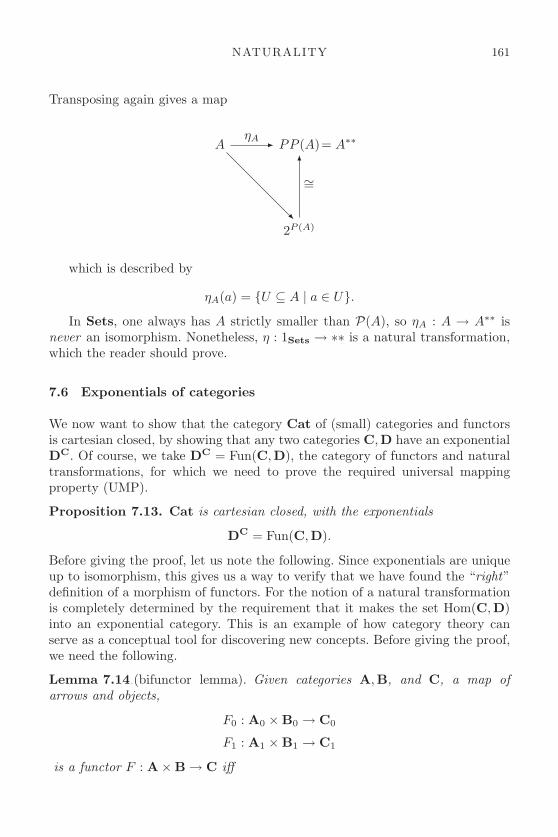
NATURALITY 161
Transposing again gives a map
AηA� PP (A)= A∗∗
2P (A)
∼=�
�
which is described by
ηA(a) = {U ⊆ A | a ∈ U}.In Sets, one always has A strictly smaller than P(A), so ηA : A → A∗∗ is
never an isomorphism. Nonetheless, η : 1Sets → ∗∗ is a natural transformation,which the reader should prove.
7.6 Exponentials of categories
We now want to show that the category Cat of (small) categories and functorsis cartesian closed, by showing that any two categories C,D have an exponentialDC. Of course, we take DC = Fun(C,D), the category of functors and naturaltransformations, for which we need to prove the required universal mappingproperty (UMP).
Proposition 7.13. Cat is cartesian closed, with the exponentials
DC = Fun(C,D).
Before giving the proof, let us note the following. Since exponentials are uniqueup to isomorphism, this gives us a way to verify that we have found the “right”definition of a morphism of functors. For the notion of a natural transformationis completely determined by the requirement that it makes the set Hom(C,D)into an exponential category. This is an example of how category theory canserve as a conceptual tool for discovering new concepts. Before giving the proof,we need the following.
Lemma 7.14.(bifunctor lemma). Given categories A,B, and C, a map ofarrows and objects,
F0 : A0 ×B0 → C0
F1 : A1 ×B1 → C1
is a functor F : A×B → C iff

162 CATEGORY THEORY
1. F is functorial in each argument: F (A,−) : B → C and F (−, B) : A → Care functors for all A ∈ A0 and B ∈ B0.
2. F satisfies the following “interchange law.” Given α : A → A′ ∈ A andβ : B → B′ ∈ B, the following commutes:
F (A,B)F (A, β)� F (A,B′)
F (A′, B)
F (α,B)
�
F (A′, β)� F (A′, B′)
F (α,B′)
�
that is, F (A′, β) ◦ F (α,B) = F (α,B′) ◦ F (A, β) in C.
Proof. (Lemma) In A×B, any arrow
〈α, β〉 : 〈A,B〉 → 〈A′, B′〉
factors as
〈A,B〉 〈1A, β〉� 〈A,B′〉
〈A′, B〉
〈α, 1B〉�
〈1A′ , β〉� 〈A′, B′〉
〈α, 1B′〉�
So (1) and (2) are clearly necessary. To show that they are also sufficient, we candefine the (proposed) functor:
F (〈A,B〉) = F (A,B)
F (〈α, β〉) = F (A′, β) ◦ F (α,B)
The interchange law, together with functoriality in each argument, then ensuresthat
F (α′, β′) ◦ F (α, β) = F (〈α′, β′〉 ◦ 〈α, β〉)

NATURALITY 163
as can be read off from the following diagram:
F (A,B)
F (A′, B)
F (α,B)
�
F (A′, β)� F (A′, B′)
F (α, β)
�
F (A′, B)
F (α′, B)
�
...................................F (A′′, β)
� F (A′′, B′)
F (α,B′)
�
F (A′′, β′)� F (A′′, B′′)
F (α′, β′)
�
Proof. (Proposition) We need to show:
1. ε = eval : Fun(C,D)×C → D is functorial.2. For any category X and functor
F : X×C → D
there is a functor
F : X → Fun(C,D)
such that ε ◦ (F × 1C) = F .3. Given any functor
G : X → Fun(C,D),
one has ˜(ε ◦ (G× 1C)) = G.
(1) Using the bifunctor lemma, we show that ε is functorial. First, fix F : C → Dand consider ε(F,−) = F : C → D. This is clearly functorial! Next, fix C ∈ C0
and consider ε(−, C) : Fun(C,D) → D defined by
(ϑ : F → G) �→ (ϑC : FC → GC).
This is also clearly functorial.For the interchange law, consider any ϑ : F → G ∈ Fun(C,D) and (f : C →
C ′) ∈ C, then we need the following to commute:
ε(F,C)ϑC� ε(G,C)
ε(F,C ′)
F (f)
�
ϑC′� ε(G,C ′)
G(f)
�

164 CATEGORY THEORY
But this holds because ε(F,C) = F (C) and ϑ is a natural transformation.The conditions (2) and (3) are now routine. For example, for (2), given
F : X×C → D
let
F : X → Fun(C,D)
be defined by
F (X)(C) = F (X,C).
7.7 Functor categories
Let us consider some particular functor categories.
Example 7.15. First, clearly C1 = C for the terminal category 1. Next, whatabout C2, where 2 = · → · is the single arrow category? This is just the arrowcategory of C that we already know,
C2 = C→.
Consider instead the discrete category, 2 = {0, 1}. Then clearly,
C2 ∼= C×C.
Similarly, for any set I (regarded as a discrete category), we have
CI ∼=∏i∈I
C.
Example 7.16. “Transcendental deduction of natural transformations”Given the possibility of functor categories DC, we can determine what the objectsand arrows therein must be as follows:
Objects: these correspond uniquely to functors of the form
1 → DC
and hence to functors
C → D.
Arrows: by the foregoing example, arrows in the functor category corresponduniquely to functors of the form
1 → (DC)2

NATURALITY 165
thus to functors of the form
2 → DC
and hence to functors
C× 2 → D
respectively
C → D2.
But a functor from C into the arrow category D2 (respectively a functor into Dfrom the cylinder category C × 2) is exactly a natural transformation betweentwo functors from C into D, as the reader can see by drawing a picture of thefunctor’s image in D.
Example 7.17. Recall that a (directed) graph can be regarded as a pair of setsand a pair of functions,
G1
t �
s� G0
where G1 is the set of edges, G0 is the set of vertices, and s and t are the sourceand target operations.
A homomorphism of graphs h : G → H is a map that preserves sources andtargets. In detail, this is a pair of functions h1 : G1 → H1 and h0 : G0 → H0
such that for all edges e ∈ G, we have sh1(e) = h0s(e) and similarly for t as well.But this amounts exactly to saying that the following two diagrams commute:
G1h1 � H1 G1
h1 � H1
G0
sG
�
h0
� H0
sH
�G0
tG
�
h0
� H0
tH
�
Now consider the category Γ, pictured as follows:
· �� ·It has exactly two objects and two distinct, parallel, nonidentity arrows. A graphG is then exactly a functor,
G : Γ → Sets
and a homomorphism of graphs h : G → H is exactly a natural transformationbetween these functors. Thus, the category of graphs is a functor category,
Graphs = SetsΓ.

166 CATEGORY THEORY
As we see later, it follows from this fact that Graphs is cartesian closed.
Example 7.18. Given a product C × D of categories, take the first productprojection
C×D → C
and transpose it to get a functor
Δ : C → CD.
For C ∈ C, the functor Δ(C) is the “constant C-valued functor,”
• Δ(C)(X) = C for all X ∈ D0
• Δ(x) = 1C for all x ∈ D1.
Moreover, Δ(f) : Δ(C) → Δ(C ′) is the natural transformation, each componentof which is f .
Now suppose we have any functor
F : D → C
and a natural transformation
ϑ : Δ(C) → F.
Then, the components of ϑ all look like
ϑD : C → F (D)
since Δ(C)(D) = C. Moreover, for any d : D → D′ in D, the usual naturalitysquare becomes a triangle, since Δ(C)(d) = 1C for all d : D → D′.
CϑD � FD
C
1C
�
ϑD′� FD′
Fd
�
Thus, such a natural transformation ϑ : Δ(C) → F is exactly a cone to thebase F (with vertex C). Similarly, a map of cones ϑ → ϕ is a constant naturaltransformation, that is, one of the form Δ(h) for some h : C → D, making acommutative triangle
Δ(C) Δ(h)� Δ(D)
F
ϕ
�
ϑ
�

NATURALITY 167
Example 7.19. Take posets P,Q and consider the functor category,
QP .
The functors Q → P , as we know, are just monotone maps, but what is a naturaltransformation?
ϑ : f → g
For each p ∈ P , we must have
ϑp : fp ≤ gp
and if p ≤ q, then there must be a commutative square involving fp ≤ fq andgp ≤ gq, which, however, is automatic. Thus, the only condition is that fp ≤ gpfor all p, that is, f ≤ g pointwise. Since this is just the usual ordering of theposet QP , the exponential poset agrees with the functor category. Thus, we havethe following.
Proposition 7.20. The inclusion functor,
Pos → Cat
preserves CCC structure.
Example 7.21. What happens if we take the functor category of two groups Gand H?
HG
Do we get an exponential of groups? Let us first ask, what is a natural transforma-tion between two group homomorphisms f, g : G → H ? Such a map ϑ : f → gwould be an element h ∈ H such that for every x ∈ G, we have
g(x) · h = h · f(x)
or, equivalently,
g(x) = h · f(x) · h−1.
Therefore, a natural transformation ϑ : f → g is an inner automorphism y �→h·y·h−1 of H (called conjugation by h) that takes f to g. Clearly, every such arrowϑ : f → g has an inverse ϑ−1 : g → f (conjugation by h−1). But HG is still notusually a group, simply because there may be many different homomorphismsG → H, so the functor category HG has more than one object.
This suggests enlarging the category of groups to include also categories withmore than one object, but still having inverses for all arrows. Such categoriesare called groupoids, and have been studied by topologists (they occur as thecollection of paths between different points in a topological space). A groupoidcan thus be regarded as a generalized group, in which the domains and codomains
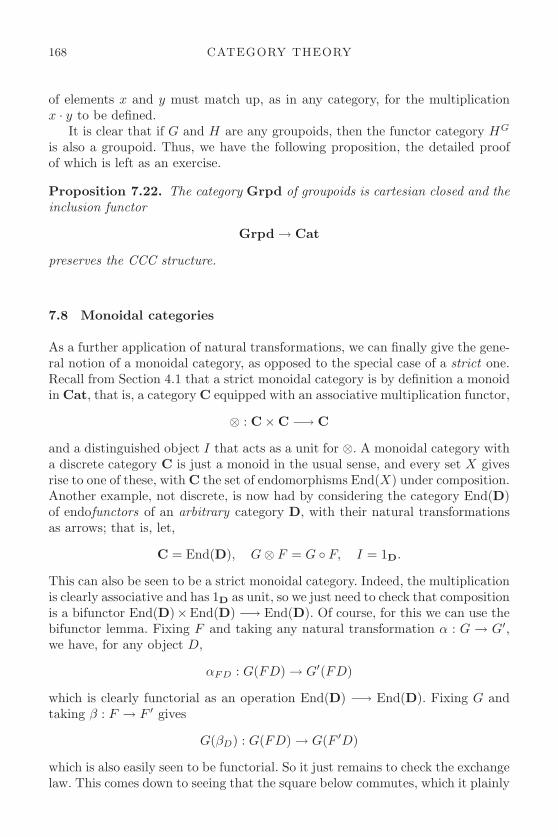
168 CATEGORY THEORY
of elements x and y must match up, as in any category, for the multiplicationx · y to be defined.
It is clear that if G and H are any groupoids, then the functor category HG
is also a groupoid. Thus, we have the following proposition, the detailed proofof which is left as an exercise.
Proposition 7.22. The category Grpd of groupoids is cartesian closed and theinclusion functor
Grpd → Cat
preserves the CCC structure.
7.8 Monoidal categories
As a further application of natural transformations, we can finally give the gene-ral notion of a monoidal category, as opposed to the special case of a strict one.Recall from Section 4.1 that a strict monoidal category is by definition a monoidin Cat, that is, a category C equipped with an associative multiplication functor,
⊗ : C×C −→ C
and a distinguished object I that acts as a unit for ⊗. A monoidal category witha discrete category C is just a monoid in the usual sense, and every set X givesrise to one of these, with C the set of endomorphisms End(X) under composition.Another example, not discrete, is now had by considering the category End(D)of endofunctors of an arbitrary category D, with their natural transformationsas arrows; that is, let,
C = End(D), G⊗ F = G ◦ F, I = 1D.
This can also be seen to be a strict monoidal category. Indeed, the multiplicationis clearly associative and has 1D as unit, so we just need to check that compositionis a bifunctor End(D)×End(D) −→ End(D). Of course, for this we can use thebifunctor lemma. Fixing F and taking any natural transformation α : G → G′,we have, for any object D,
αFD : G(FD) → G′(FD)
which is clearly functorial as an operation End(D) −→ End(D). Fixing G andtaking β : F → F ′ gives
G(βD) : G(FD) → G(F ′D)
which is also easily seen to be functorial. So it just remains to check the exchangelaw. This comes down to seeing that the square below commutes, which it plainly

NATURALITY 169
does just because α is natural.
GFDαFD� G′FD
GF ′D
GβD
�
αF ′D
� G′F ′D
G′βD
�
Some of the other examples of strict monoidal categories that we have seeninvolved “product-like” operations such as meets a ∧ b and joins a ∨ b in posets.We would like to also capture general products A×B and coproducts A + B incategories having these; however, these operations are not generally associativeon the nose, but only up to isomorphism. Specifically, given any three objectsA,B,C in a category with all finite products, we do not have A × (B × C) =(A×B)× C, but instead an isomorphism,
A× (B × C) ∼= (A×B)× C.
Note, however, that there is exactly one such isomorphism that commuteswith all three projections, and it is natural in all three arguments. Similarly,taking a terminal object 1, rather than 1 × A = A = A × 1, we have naturalisomorphisms,
1×A ∼= A ∼= A× 1
which, again, are uniquely determined by the condition that they commute withthe projections. This leads us to the following definition.
Definition 7.23. A monoidal category consists of a category C equipped witha functor
⊗ : C×C −→ C
and a distinguished object I, together with natural isomorphisms,
αABC : A⊗ (B ⊗ C) ∼−→ (A⊗B)× C,
λA : I ⊗A∼−→ A, ρA : A⊗ I
∼−→ A.
Moreover, these are required to always make the following diagrams commute:

170 CATEGORY THEORY
(A⊗B)⊗ (C ⊗D)
A⊗ (B ⊗ (C ⊗D))
α
�
((A⊗B)⊗ C)⊗D
α
�
A⊗ ((B ⊗ C)⊗D)
1⊗ α
�
α� (A⊗ (B ⊗ C))⊗D
α⊗ 1�
(“Mac Lane’s pentagon”)
A⊗ (I ⊗A)α � (A⊗ I)⊗A
A⊗A
ρA ⊗ 1
�
1⊗ λA �
I ⊗ I ================== I ⊗ I
I
ρI
�
λI�
In this precise sense, a monoidal category is thus a category that is strictmonoidal “up to natural isomorphism”—where the natural isomorphisms arespecified and compatible. An example is, of course, a category with all finiteproducts, where the required equations above are ensured by the UMP of pro-ducts and the selection of the maps α, λ, ρ as the unique ones commuting withprojections. We leave the verification as an exercise. The reader familiar with ten-sor products of vector spaces, modules, rings, etc., will have no trouble verifyingthat these, too, give examples of monoidal categories.
A further example comes from an unexpected source: linear logic. The logicaloperations of linear conjunction and disjunction, sometimes written P ⊗Q andP⊕Q, can be modeled in a monoidal category, usually with extra structure σAB :A ⊗ B
∼−→ B ⊗ A making these operations “symmetric” (up to isomorphism).Here, too, we leave the verification to the reader familiar with this logical system.
The basic theorem regarding monoidal categories is Mac Lane’s coherencetheorem, which says that “all diagrams commute.” Somewhat more precisely, it

NATURALITY 171
says that any diagram in a monoidal category constructed, like those above, justfrom identities, the functor ⊗, and the maps α, λ, ρ will necessarily commute. Weshall not state the theorem more precisely than this, nor will we give its some-what technical proof which, surprisingly, uses ideas from proof theory relatedto Gentzen’s cut elimination theorem! The details can be found in Mac Lane’sbook, Categories Work.
7.9 Equivalence of categories
Before examining some particular functor categories in more detail, we considerone very special application of the concept of natural isomorphism. Consider firstthe following situation.
Example 7.24. Let Ordfin be the category of finite ordinal numbers. Thus, theobjects are the sets 0, 1, 2, . . . , where 0 = ∅ and n = {0, . . . , n − 1}, while thearrows are all functions between these sets. Now suppose that for each finite setA we select an ordinal |A| that is its cardinal and an isomorphism,
A ∼= |A|.
Then for each function f : A → B of finite sets, we have a function |f | bycompleting the square
A∼= � |A|
B
f
�
∼=� |B|
|f |�
................
(7.2)
This clearly gives us a functor
| − | : Setsfin → Ordfin.
Actually, all the maps in the above square are in Setsfin; so we should also makethe inclusion functor
i : Ordfin → Setsfin
explicit. Then we have the selected isos,
ϑA : A∼→ i|A|
and we know by (7.2) that
i(|f |) ◦ ϑA = ϑB ◦ f.

172 CATEGORY THEORY
This, of course, says that we have a natural isomorphism
ϑ : 1Setsfin → i ◦ | − |between two functors of the form
Setsfin → Setsfin.
On the other hand, if we take an ordinal and take its ordinal, we get nothingnew,
|i(−)| = 1Ordfin : Ordfin → Ordfin.
This is so because, for any finite ordinal n,
|i(n)| = n
and we can assume that we take ϑn = 1n : n → |i(n)|, so that also,
|i(f)| = f : n → m.
In sum, then, we have a situation where two categories are very similar; butthey are not the same and they are not even isomorphic (why?). This kind ofcorrespondence is what is captured by the notion of equivalence of categories.
Definition 7.25. An equivalence of categories consists of a pair of functors
E : C → D
F : D → C
and a pair of natural isomorphisms
α : 1C∼→ F ◦ E in CC
β : 1D∼→ E ◦ F in DD.
In this situation, the functor F is called a pseudo-inverse of E. The categoriesC and D are then said to be equivalent, written C # D.
Observe that equivalence of categories is a generalization of isomorphism.Indeed, two categories C,D are isomorphic if there are functors.
E : C → D
F : D → C
such that
1C = F ◦ E
1D = E ◦ F.
In the case of equivalence C # D, we replace the identity natural transfor-mations by natural isomorphisms. In that sense, equivalence of categories as“isomorphism up to isomorphism.”

NATURALITY 173
Experience has shown that the mathematically significant properties ofobjects are those that are invariant under isomorphisms, and in category theory,identity of objects is a much less important relation than isomorphism. So it isreally equivalence of categories that is the more important notion of “similarity”for categories.
In the foregoing example Setsfin # Ordfin, we see that every set is isomorphicto an ordinal, and the maps between ordinals are just the maps between themas sets. Thus, we have
1. for every set A, there is some ordinal n with A ∼= i(n),2. for any ordinals n,m, there is an isomorphism,
HomOrdfin(n,m) ∼= HomSetsfin(i(n), i(m))
where i : Ordfin → Setsfin is the inclusion functor.
In fact, these conditions are characteristic of equivalences, as the followingproposition shows.
Proposition 7.26. The following conditions on a functor F : C → D areequivalent:
1. F is (part of) an equivalence of categories.2. F is full and faithful and “essentially surjective” on objects: for every D∈D
there is some C ∈ C such that FC ∼= D.
Proof. (1 implies 2) Take E : D → C, and
α : 1C∼→ EF
β : 1D∼→ FE.
In C, for any C, we then have αC : C∼→ EF (C), and
CαC� EF (C)
C ′
f
�
αC′� EF (C ′)
EF (f)
�
commutes for any f : C → C ′.Thus, if F (f) = F (f ′), then EF (f) = EF (f ′), so f = f ′. So F is faithful.
Note that by symmetry, E is also faithful.Now take any arrow
h : F (C) → F (C ′) in D,

174 CATEGORY THEORY
and consider
C∼= � EF (C)
C ′
f
�
∼=� EF (C ′)
E(h)
�
where f = (αC′)−1 ◦ E(h) ◦ αC . Then, we have also F (f) : F (C) → F (C ′) and
EF (f) = E(h) : EF (C) → EF (C ′)
by the naturality square
CαC� EF (C)
C ′
f
�
αC′� EF (C ′)
EF (f)
�
Since E is faithful, F (f) = h. So F is also full.Finally, for any object D ∈ D, we have
β : 1D∼→ FE
so
βD : D ∼= F (ED), for ED ∈ C0.
(2 implies 1) We need to define E : D → C and natural transformations,
α : 1C∼→ EF
β : 1D∼→ FE.
Since F is essentially surjective, for each D ∈ D0, we can choose some E(D) ∈ C0
along with some βD : D∼→ FE(D). That gives E on objects and the proposed
components of β : 1D → FE.Given h : D → D′ in D, consider
DβD � FE(D)
D′
h
�
βD′� FE(D′)
βD′ ◦ h ◦ β−1D
�
................

NATURALITY 175
Since F : C → D is full and faithful, there is a unique arrow
E(h) : E(D) → E(D′)
with FE(h) = βD′ ◦ h ◦ β−1D . It is easy to see that then E : D → C is a functor
and β : 1D∼→ FE is clearly a natural isomorphism.
To find α : 1C → EF , apply F to any C and consider βFC : F (C) →FEF (C). Since F is full and faithful, the preimage of βFC is an isomorphism,
αC = F−1(βFC) : C∼→ EF (C)
which is easily seen to be natural, since β is.
7.10 Examples of equivalence
Example 7.27. Pointed sets and partial mapsLet Par be the category of sets and partial functions. An arrow
f : A ⇁ B
is a function |f | : Uf → B for some Uf ⊆ A. Identities in Par are the same asthose in Sets, that is, 1A is the total identity function on A. The compositeof f : A ⇁ B and g : B ⇁ C is given as follows: Let U(g◦f) := f−1(Ug) ⊆ A,and |g ◦ f | : U(g◦f) → C is the horizontal composite indicated in the followingdiagram, in which the square is a pullback:
|f |−1(Ug) � Ug |g|� C
Uf
�
∩
|f |� B
�
∩
A�
∩
It is easy to see that composition is associative and that the identities are units,so we have a category Par.
The category of pointed sets,
Sets∗
has as objects, sets A equipped with a distinguished “point” a ∈ A, that is, pairs,
(A, a) with a ∈ A.

176 CATEGORY THEORY
Arrows are functions that preserve the point, that is, an arrow f : (A, a) → (B, b)is a function f : A → B such that f(a) = b.
Now we show:
Proposition 7.28. Par # Sets∗
The functors establishing the equivalence are as follows:
F : Par → Sets∗
is defined on an object A by F (A) = (A ∪ {∗}, ∗), where ∗ is a new elementthat we add to A. We also write A∗ = A ∪ {∗}. For arrows, given f : A ⇁ B,F (f) : A∗ → B∗ is defined by
f∗(x) =
{f(x) if x ∈ Uf
∗ otherwise.
Then clearly f∗(∗A) = ∗B , so in fact f∗ : A∗ → B∗ is “pointed,” as required.Coming back, the functor
G : Sets∗ → Par
is defined on an object (A, a) by G(A, a) = A−{a} and for an arrow f : (A, a) →(B, b)
G(f) : A− {a} ⇁ B − {b}is the function with domain
UG(f) = A− f−1(b)
defined by G(f)(x) = f(x) for every f(x) �= b.Now G ◦ F is the identity on Par, because we are just adding a new point
and then throwing it away. But F ◦ G is only naturally isomorphic to 1Sets∗ ,since we have
(A, a) ∼= ((A− {a}) ∪ {∗}, ∗).These sets are not equal, since a �= ∗. It still needs to be checked,
of course, that F and G are functorial, and that the comparison (A, a) ∼=((A − {a}) ∪ {∗}, ∗) is natural, but we leave these easy verifications to thereader.
Observe that this equivalence implies that Par has all limits, since it is equi-valent to a category of “algebras” of a very simple type, namely sets equippedwith a single, nullary operation, that is, a “constant.” We already know thatlimits of algebras can always be constructed as limits of the underlying sets, andan easy exercise shows that a category equivalent to one with limits of any typealso has such limits.

NATURALITY 177
Example 7.29. Slice categories and indexed familiesFor any set I, the functor category SetsI is the category of I-indexed sets.
The objects are I-indexed families of sets
(Ai)i∈I
and the arrows are I-indexed families of functions,
(fi : Ai → Bi)i∈I : (Ai)i∈I −→ (Bi)i∈I .
This category has an equivalent description that is often quite useful: it is equi-valent to the slice category of Sets over I, consisting of arrows α : A → I and“commutative triangles” over I (see Section 1.6),
SetsI # Sets/I.
Indeed, define functors
Φ : SetsI −→ Sets/I
Ψ : Sets/I −→ SetsI
on objects as follows:
Φ((Ai)i∈I) = π :∐i∈I
Ai → I (the indexing projection),
where the coproduct is conveniently taken to be∐i∈I
Ai = {(i, a) | a ∈ Ai}.
And coming back, we have
Ψ(α : A → I) = (α−1{i})i∈I .
The effect on arrows is analogous and easily inferred. We leave it as an exerciseto show that these are indeed mutually pseudo-inverse functors. (Why are theynot inverses?)
The equivalent description of SetsI as Sets/I leads to the idea that, for ageneral category E , the slice category E/X, for any object X, can also be regardedas the category of “X-indexed objects of E”, although the functor category EX
usually does not make sense. This provides a precise notion of an “X-indexedfamily of objects Ex of E ,” namely as a map E → X.
For instance, in topology, there is the notion of a “fiber bundle” as a conti-nuous function π : Y → X, thought of as a family of spaces Yx = π−1(x), the“fibers” of π, varying continuously in a parameter x ∈ X. Similarly, in dependenttype theory there are “dependent types” x : X A(x), thought of as families oftypes indexed over a type. These can be modeled as objects [[A]] → [[X]] in the

178 CATEGORY THEORY
slice category E/[[X]] over the interpretation of the (closed) type X as an objectof a category E .
If E has pullbacks, reindexing of an “indexed family” along an arrow f :Y → X in E is represented by the pullback functor f∗ : E/X → E/Y . Thisis motivated by the fact that in Sets the following diagram commutes (up tonatural isomorphism) for any f : J → I:
SetsI #� Sets/I
SetsJ
Setsf
�
#� Sets/J
f∗
�
where the functor Setsf is the reindexing along f :
(Setsf (Ai))j = Af(j).
Moreover, there are also functors going in the other direction,
Σf ,Πf : Sets/J −→ Sets/I
which, in terms of indexed families, are given by taking sums and products ofthe fibers:
(Σf (Aj))i =∑
f(j)=i
Aj
and similarly for Π. These functors can be characterized in terms of the pullbackfunctor f∗ (as adjoints, see Section 9.7), and so also make sense in categories moregeneral than Sets, where there are no “indexed families” in the usual sense. Forinstance, in dependent type theory, these operations are formalized by logicalrules of inference similar to those for the existential and universal quantifier,and the resulting category of types has such operations of dependent sums andproducts.
Example 7.30. Stone dualityMany examples of equivalences of categories are given by what are called “dua-lities.” Often, classical duality theorems are not of the form C ∼= Dop (muchless C = Dop), but rather C # Dop, that is, C is equivalent to the opposite(or “dual”) category of D. This is because the duality is established by a con-struction that returns the original thing only up to isomorphism, not “on thenose.” Here is a simple example, which is a very special case of the far-reachingStone duality theorem.
Proposition 7.31. The category of finite Boolean algebras is equivalent to theopposite of the category of finite sets,
BAfin # Setsopfin.

NATURALITY 179
Proof. The functors involved here are the contravariant powerset functor
PBA : Setsopfin → BAfin
on one side (the powerset of a finite set is finite!). Going back, we use the functor,
A : BAopfin → Setsfin
taking the set of atoms of a Boolean algebra,
A(B) = {a ∈ B | 0 < a and (b < a ⇒ b = 0)}.
In the finite case, this is isomorphic to the ultrafilter functor that we have alreadystudied (see Section 7.3).
Lemma 7.32. For any finite Boolean algebra B, there is an isomorphismbetween atoms a in B and ultrafilters U ⊆ B, given by
U �→∧b∈U
b
and
a �→ ↑(a).
Proof. If a is an atom, then ↑(a) is an ultrafilter, since for any b either a∧ b = aand then b ∈↑(a) or a ∧ b = 0 and so ¬b ∈↑(a).
If U ⊆ B is an ultrafilter then 0 <∧
b∈U b, because, since U is finite andclosed under intersections, we must have
∧b∈U b ∈ U . If 0 �= b0 <
∧b∈U b then
b0 is not in U , so ¬b0 ∈ U . But then b0 < ¬b0 and so b0 = 0.Plainly, U ⊆↑ (
∧b∈U b) since b ∈ U implies
∧b∈U b ⊆ b. Now let
∧b∈U b ≤ a
for some a not in U . Then, ¬a ∈ U implies that also∧
b∈U b ≤ ¬a, and so∧b∈U b ≤ a ∧ ¬a = 0, which is impossible.
Since we know that the set of ultrafilters Ult(B) is contravariantly functorial(it is represented by the Boolean algebra 2, see Section 7.3), we therefore alsohave a contravariant functor of atoms A ∼= Ult. The explicit description of thisfunctor is this: if h : B → B′ and a′ ∈ A(B′), then it follows from the lemma thatthere is a unique atom a ∈ B such that a′ ≤ h(b) iff a ≤ b for all b ∈ B. To findthis atom a, take the intersection over the ultrafilter h−1(↑(a′)),
A(a′) = a =∧
a′≤h(b)
b.
Thus, we get a function
A(h) : A(B′) → A(B).

180 CATEGORY THEORY
Of course, we must still check that this is a pseudo-inverse for PBA : Setsopfin →
BAfin. The required natural isomorphisms,
αX : X → A(P(X))
βB : B → P(A(B))
are explicitly described as follows:The atoms in a finite powerset P(X) are just the singletons {x} for x ∈ X,
thus αX(x) = {x} is clearly an isomorphism.To define βB, let
βB(b) = {a ∈ A(B) | a ≤ b}.
To see that βB is also iso, consider the proposed inverse,
(βB)−1(B) =∨
a∈B
a for B ⊆ A(B).
The isomorphism then follows from the following lemma, the proof of which isroutine.
Lemma 7.33. For any finite Boolean algebra B,
1. b =∨{a ∈ A(B) | a ≤ b}.
2. If a is an atom and a ≤ b ∨ b′, then a ≤ b or a ≤ b′.
Of course, one must still check that α and β really are natural transformati-ons. This is left to the reader.
Finally, we remark that the duality
BAfin # Setsopfin
extends to one between all sets on the one side and the complete, atomic Booleanalgebras, on the other,
caBA # Setsop,
where a Boolean algebra B is complete if every subset U ⊆ B has a join∨
U ∈ Band a complete homomorphism preserves these joins and B is atomic if everynonzero element 0 �= b ∈ B has some a ≤ b with a an atom.
Moreover, this is just the discrete case of the full Stone duality theo-rem, which states an equivalence between the category of all Boolean algebrasand the opposite of a certain category of topological spaces, called “Stonespaces,” and all continuous maps between them. For details, see Johnstone(1982).

NATURALITY 181
7.11 Exercises
1. Consider the (covariant) composite functor,
F = PBA ◦Ultop : BA → Setsop → BA
taking each Boolean algebra B to the powerset algebra of sets of ultrafiltersin B. Note that
F(B) ∼= HomSets(HomBA(B,2), 2)
is a sort of “double-dual” Boolean algebra. There is always ahomomorphism,
φB : B → F(B)
given by φB(b) = {V ∈ Ult(B) | b ∈ V}. Show that for any Booleanhomomorphism h : A → B, the following square commutes:
AφA � F(A)
B
h
�
φB
� F(B)
F(h)
�
2. Show that the homomorphism φB : B → F(B) in the foregoing problem isalways injective (use the Boolean prime ideal theorem). This is the classi-cal “Stone representation theorem,” stating that every Boolean algebra isisomorphic to a “field of sets,” that is, a sub-Boolean algebra of a powerset.Is the functor F faithful?
3. Prove that for any finite Boolean algebra B, the “Stone representation”
φ : B → P(Ult(B))
is in fact an isomorphism of Boolean algebras. (Note the similarity to thecase of finite dimensional vector spaces.) This concludes the proof that wehave an equivalence of categories,
BAfin # Setsopfin
This is the “finite” case of Stone duality.4. Consider the forgetful functors
Groups U−→ Monoids V−→ Sets

182 CATEGORY THEORY
Say whether each is faithful, full, injective on arrows, surjective on arrows,injective on objects, and surjective on objects.
5. Make every poset (X,≤) into a topological space by letting U ⊆ X beopen just if x ∈ U and x ≤ y implies y ∈ U (U is “closed upward”). Thisis called the Alexandroff topology on X. Show that it gives a functor
A : Pos → Top
from posets and monotone maps to spaces and continuous maps by showingthat any monotone map of posets f : P → Q is continuous with respectto this topology on P and Q (the inverse image of an open set must beopen).
Is A faithful? Is it full?6. Prove that every functor F : C → D can be factored as D ◦ E = F ,
C E−→ E D−→ D
in the following two ways:
(a) E : C → E is bijective on objects and full, and D : E → D is faithful;(b) E : C → E surjective on objects and D : E → D is injective on objects
and full and faithful.
When do the two factorizations agree?7. Show that a natural transformation is a natural isomorphism just if
each of its components is an isomorphism. Is the same true for mono-morphisms?
8. Show that a functor category DC has binary products if D does (constructthe product of two functors F and G “objectwise”: (F ×G)(C) = F (C)×G(C)).
9. Show that the map of sets
ηA : A −→ PP (A)
a �−→ {U ⊆ A|a ∈ U}is the component at A of a natural transformation η : 1Sets → PP , whereP : Setsop → Sets is the (contravariant) powerset functor.
10. Let C be a locally small category. Show that there is a functor
Hom : Cop ×C → Sets
such that for each object C of C,
Hom(C,−) : C → Sets
is the covariant representable functor and
Hom(−, C) : Cop → Sets

NATURALITY 183
is the contravariant one. (Hint: use the bifunctor lemma.)11. Recall from the text that a groupoid is a category in which every arrow is
an isomorphism. Prove that the category of groupoids is cartesian closed.12. Let C ∼= D be equivalent categories. Show that C has binary products if
and only if D does.13. What sorts of properties of categories do not respect equivalence? Find
one that respects isomorphism, but not equivalence.14. Complete the proof that Par ∼= Sets∗.15. Show that equivalence of categories is an equivalence relation.16. A category is skeletal if isomorphic objects are always identical. Show that
every category is equivalent to a skeletal subcategory. (Every category hasa “skeleton.”)
17. Complete the proof that, for any set I, the category of I-indexed familiesof sets, regarded as the functor category SetsI , is equivalent to the slicecategory Sets/I of sets over I,
SetsI # Sets/I.
Show that reindexing of families along a function f : J → I, given byprecomposition,
Setsf ((Ai)i∈I) = (Af(j))j∈J
is represented by pullback, in the sense that the following diagram ofcategories and functors commutes up to natural isomorphism:
SetsI #� Sets/I
SetsJ
Setsf
�
#� Sets/J
f∗
�
Here f∗ : Sets/J → Sets/I is the pullback functor along f : J → I.Finally, infer that Sets/2 # Sets × Sets, and similarly for any n otherthan 2.
18. Show that a category with finite products is a monoidal category. Inferthat the same is true for any category with finite coproducts.

This page intentionally left blank

8
CATEGORIES OF DIAGRAMS
In this chapter, we prove a very useful technical result called the Yoneda lemma,and then employ it in the study of the important categories of set-valued functorsor “diagrams.” The Yoneda lemma is perhaps the single most used result incategory theory. It can be seen as a straightforward generalization of some simplefacts about monoids and posets, yet it has much more far-reaching applications.
8.1 Set-valued functor categories
We are going to focus on special functor categories of the form
SetsC
where the category C is locally small. Thus, the objects are set-valued functors,
F,G : C → Sets
(sometimes called “diagrams on C”), and the arrows are natural transformations
α, β : F → G.
Where C = P, a poset, we have already considered such functors as “variablesets,” that is, sets Fi depending on a parameter i ∈ P. The general case of anon-poset C similarly admits an interpretation as “variable sets”: such a functorF gives a family of sets FC and transitions FC → FC ′ showing how the setschange according to every C → C ′. For instance, C might be the category Setsfin
of all finite sets (of finite sets, ...) and all functions between them. Then inSetsSetsfin there is for example the inclusion functor U : Setsfin → Sets, whichcan be regarded as a “generic” or variable finite set, along with the functorsU × U , U + U , etc., which are “variable” structures of these kinds.
Given any such category SetsC, remember that we can evaluate anycommutative diagram,
Pα � Q
R
β
�βα
�

186 CATEGORY THEORY
at any object C to get a commutative diagram in Sets,
PCαC � QC
RC
βC
�(βα)C �
(8.1)
Thus, for each object C, there is an evaluation functor
evC : SetsC → Sets.
Moreover, naturality means that if we have any arrow f : D → C, we get a“cylinder” over the diagram (8.1) in Sets.
Another way of thinking about such functor categories that was already con-sidered in Section 7.7 is suggested by considering the case where C is the categoryΓ pictured as
1 �� 0
Then a set-valued functor G : Γ → Sets is just a graph, and a naturaltransformation α : G → H is a graph homomorphism. Thus, for this case,
SetsΓ = Graphs.
This suggests regarding an arbitrary category of the form SetsC as a generalized“category of structured sets” and their “homomorphisms”; indeed, this is a veryuseful way of thinking of such functors and their natural transformations.
Another basic example is the category SetsΔop, where the index category Δ
is the category of finite ordinals that we already met in Chapter 7. The objectsof SetsΔop
are called simplicial sets, and are used in topology to compute thehomology, cohomology, and homotopy of spaces. Since Δ looks like
0 � 1�� � 2
�� �� �3 . . .
(satisfying the simplicial identities), a simplicial set S : Δop → Sets looks likethis:
S0� S1
� �� S2
� �� ��S3 . . .
(satisfying the corresponding identities). For example, one can take Sn = Sn =S× . . .×S (n times) for a fixed set S to get a (rather trivial) simplicial set, withthe maps being the evident product projections and generalized diagonals. Moreinterestingly, for a fixed poset P, one takes
S(P)n = {(p1, . . . , pn) ∈ Pn | p1 ≤ . . . ≤ pn},with the evident projections and inclusions; this is called the “simplicial nerve”of the poset P.

CATEGORIES OF DIAGRAMS 187
8.2 The Yoneda embedding
Among the objects of SetsC are certain very special ones, namely the (covariant)representable functors,
HomC(C,−) : C → Sets.
Observe that for each h : C → D in C, we have a natural transformation
HomC(h,−) : HomC(D,−) → HomC(C,−)
(note the direction!) where the component at X is defined by precomposition:
(f : D → X) �→ (f ◦ h : C → X).
Thus, we have a contravariant functor
k : Cop → SetsC
defined by k(C) = HomC(C,−). Of course, this functor k is just the exponentialtranspose of the bifunctor
HomC : Cop ×C → Sets
which was shown as an exercise to be functorial.If we instead transpose HomC with respect to its other argument, we get a
covariant functor,
y : C → SetsCop
from C to a category of contravariant set-valued functors, sometimes called“presheaves.” (Or, what amounts to the same thing, we can put D = Cop andapply the previous considerations to D in place of C.) More formally:
Definition 8.1. The Yoneda embedding is the functor y : C → SetsCop
takingC ∈ C to the contravariant representable functor,
yC = HomC(−, C) : Cop → Sets
and taking f : C → D to the natural transformation,
yf = HomC(−, f) : HomC(−, C) → HomC(−, D).
A functor F : C → D is called an embedding if it is full, faithful, and injectiveon objects. We soon show that y really is an embedding; this is a corollary ofthe Yoneda lemma.
One should thus think of the Yoneda embedding y as a “representation” of Cin a category of set-valued functors and natural transformations on some indexcategory. Compared to the Cayley representation considered in Section 1.5, thishas the virtue of being full : any map ϑ : yC → yD in SetsC
opcomes from

188 CATEGORY THEORY
a unique map h : C → D in C as yh = ϑ. Indeed, recall that the Cayleyrepresentation of a group G was an injective group homomorphism
G � Aut(|G|) ⊆ |G||G|
where each g ∈ G is represented as an automorphism g of the set |G| of elements(i.e., a “permutation”), by letting it “act on the left,”
g(x) = g · xand the group multiplication is represented by composition of permutations,
g · h = g ◦ h.
We also showed a generalization of this representation to arbitrary categories.Thus for any monoid M , there is an analogous representation
M � End(|M |) ⊆ |M ||M |
by left action, representing the elements of M as endomorphisms of |M |.Similarly, any poset P can be represented as a poset of subsets and inclusions
by considering the poset Low(P ) of “lower sets” A ⊆ P , that is, subsets that are“closed down” in the sense that a′ ≤ a ∈ A implies a′ ∈ A, ordered by inclusion.Taking the “principal lower set”
↓(p) = {q ∈ P | q ≤ p}of each element p ∈ P determines a monotone injection
↓ : P � Low(P ) ⊆ P(|P |)such that p ≤ q iff ↓(p) ⊆ ↓(q).
The representation given by the Yoneda embedding is closely related to these,but “better” in that it cuts down the arrows in the codomain category to justthose in the image of the representation functor y : C → SetsC
op(since y is
full). Indeed, there may be many automorphisms α : G → G of a group G thatare not left actions by an element, but if we require α to commute with all rightactions α(x · g) = α(x) · g, then α must itself be a left action. This is what theYoneda embedding does in general; it adds enough “structure” to the objects yAin the image of the representation that the only “homomorphisms” ϑ : yA → yBbetween those objects are the representable ones ϑ = yh for some h : A → B. Inthis sense, the Yoneda embedding y represents the objects and arrows of C ascertain “structured sets” and (all of ) their “homomorphisms.”
8.3 The Yoneda lemma
Lemma 8.2.(Yoneda). Let C be locally small. For any object C ∈ C and functorF ∈ Sets,C
opthere is an isomorphism
Hom(yC, F ) ∼= FC

CATEGORIES OF DIAGRAMS 189
which, moreover, is natural in both F and C.
Here
(1) the Hom is HomSetsCop ,
(2) naturality in F means that, given any ϑ : F → G, the following diagramcommutes:
Hom(yC, F )∼=� FC
Hom(yC,G)
Hom(yC, ϑ)
�
∼=� GC
ϑC
�
(3) naturality in C means that, given any h : C → D, the following diagramcommutes:
Hom(yC, F )∼=� FC
Hom(yD,F )
Hom(yh, F )�
∼=� FD
Fh
�
Proof. To define the desired isomorphism,
ηC,F : Hom(yC, F )∼=−→ FC
take ϑ : yC → F and let
ηC,F (ϑ) = ϑC(1C)
which we also write as
xϑ = ϑC(1C) (8.2)
where ϑC : C(C,C) → FC and so ϑC(1C) ∈ FC.Conversely, given any a ∈ FC, we define the natural transformation ϑa :
yC → F as follows. Given any C ′, we define the component
(ϑa)C′ : Hom(C ′, C) → FC ′
by setting
(ϑa)C′(h) = F (h)(a) (8.3)
for h : C ′ → C.

190 CATEGORY THEORY
To show that ϑa is natural, take any f : C ′′ → C ′, and consider the followingdiagram:
Hom(C ′′, C)(ϑa)C′′� FC ′′
Hom(C ′, C)
Hom(f, C)�
(ϑa)C′� FC ′
F (f)
�
We then calculate, for any h ∈ yC(C ′)
(ϑa)C′′ ◦Hom(f, C)(h) = (ϑa)C′′(h ◦ f)
= F (h ◦ f)(a)
= F (f) ◦ F (h)(a)
= F (f)(ϑa)C′(h).
So ϑa is indeed natural.Now to show that ϑa and xϑ are mutually inverse, let us calculate ϑxϑ
for agiven ϑ : yC → F . First, just from the definitions (8.2) and (8.3), we have thatfor any h : C ′ → C,
(ϑ(xϑ))C′(h) = F (h)(ϑC(1C)).
But since ϑ is natural, the following commutes:
yC(C)ϑC� FC
yC(C ′)
yC(h)
�
ϑC′� FC ′
Fh
�
So, continuing,
(ϑ(xϑ))C′(h) = F (h)(ϑC(1C))
= ϑC′ ◦ yC(h)(1C)
= ϑC′(h).
Therefore, ϑ(xϑ) = ϑ.

CATEGORIES OF DIAGRAMS 191
Going the other way around, for any a ∈ FC, we have
xϑa= (ϑa)C(1C)
= F (1C)(a)
= 1FC(a)
= a.
Thus, Hom(yC, F ) ∼= FC, as required.The naturality claims are also easy: given φ : F → F ′, taking ϑ ∈
Hom(yC, F ), and chasing around the diagram
Hom(yC, F )ηC,F� FC
Hom(yC, F ′)
Hom(yC, φ)
�
ηC,F ′� F ′C
φC
�
we get
φC(xϑ) = φC(ϑC(1C))
= (φϑ)C(1C)
= x(φϑ)
= ηC,F ′(Hom(yC, φ)(ϑ)).
For naturality in C, take some f : C ′ → C. We then have
ηC′(yf)∗(ϑ) = ηC′(ϑ ◦ yf)
= (ϑ ◦ yf)C′(1C′)
= ϑC′ ◦ (yf)C′(1C′)
= ϑC′(f ◦ 1C′)
= ϑC′(f)
= ϑC′(1C ◦ f)
= ϑC′ ◦ (yC)(f)(1C)
= F (f) ◦ ϑC(1C)
= F (f)ηC(ϑ).

192 CATEGORY THEORY
The penultimate equation is by the naturality square:
yC(C)ϑC� F (C)
yC(C ′)
yC(f)
�
ϑC′� F (C ′)
F (f)
�
Therefore, ηC′ ◦ (yf)∗ = F (f) ◦ ηC .
The Yoneda lemma is used to prove our first “theorem.”
Theorem 8.3. The Yoneda embedding y : C → SetsCop
is full and faithful.
Proof. For any objects C,D ∈ C, we have an isomorphism
HomC(C,D) = yD(C) ∼= HomSetsCop (yC, yD).
And this isomorphism is indeed induced by the functor y, since by (8.3) it takesan element h : C → D of yD(C) to the natural transformation ϑh : yC → yDgiven by
(ϑh)C′(f : C ′ → C) = yD(f)(h)
= HomC(f,D)(h)
= h ◦ f
= (yh)C′(f),
where yh : yC → yD has component at C ′:
(yh)C′ : Hom(C ′, C) −→ Hom(C ′, D)
f �−→ h ◦ f
So, ϑh = y(h).
Remark 8.4. Note the following:
• If C is small, then SetsCop
is locally small, and so Hom(yC, P ) in SetsCop
is a set.
• If C is locally small, then SetsCop
need not be locally small. In this case,the Yoneda lemma tells us that Hom(yC, P ) is always a set.
• If C is not locally small, then y : C → SetsCop
will not even be defined, sothe Yoneda lemma does not apply.
Finally, observe that the Yoneda embedding y : C → SetsCop
is also injectiveon objects. For, given objects A,B in C, if yA = yB then 1C ∈ Hom(C,C) =yC(C) = yD(C) = Hom(C,D) implies C = D.

CATEGORIES OF DIAGRAMS 193
8.4 Applications of the Yoneda lemma
One frequent sort of application of the Yoneda lemma is of the following form:given objects A,B in a category C, to show that A ∼= B it suffices to showthat yA ∼= yB in SetsC
op. This “Yoneda principle” results from the foregoing
theorem and the fact that, if F : C → D is any full and faithful functor, thenFA ∼= FB clearly implies A ∼= B. We record this as the following.
Corollary 8.5 (Yoneda principle). Given objects A and B in any locallysmall category C,
yA ∼= yB implies A ∼= B.
A typical such case is this. In any cartesian closed category C, we know thereis always an isomorphism,
(AB)C ∼= A(B×C),
for any objects A,B,C. But recall how involved it was to prove this directly,using the compound universal mapping property (or a lengthy calculation inλ-calculus). Now, however, by the Yoneda principle, we just need to show that
y((AB)C) ∼= y(A(B×C)).
To that end, take any object X ∈ C; then we have isomorphisms:
Hom(X, (AB)C) ∼= Hom(X × C,AB)∼= Hom((X × C)×B,A)∼= Hom(X × (B × C), A)
∼= Hom(X,A(B×C)).
Of course, it must be checked that these isomorphisms are natural in X, but thatis straightforward. For instance, for the first one suppose we have f : X ′ → X.Then, the naturality of the first isomorphism means that for any g : X → (AB)C ,we have
g ◦ f = g ◦ (f × 1),
which is clearly true by the uniqueness of transposition (the reader should drawthe diagram).
Here is another sample application of the Yoneda principle.
Proposition 8.6. If the cartesian closed category C has coproducts, then C is“distributive,” that is, there is always a canonical isomorphism,
(A×B) + (A× C) ∼= A× (B + C).

194 CATEGORY THEORY
Proof. As in the previous proposition, we check that
Hom(A× (B + C), X) ∼= Hom(B + C,XA)
∼= Hom(B,XA)×Hom(C,XA)∼= Hom(A×B,X)×Hom(A× C,X)∼= Hom((A×B) + (A× C), X).
Finally, as in the foregoing example, one sees easily that these isos are all naturalin X.
We have already used a simple logical version of the Yoneda lemma severaltimes: to show that in the propositional calculus one has ϕ ! ψ for someformulas ϕ,ψ, it suffices to show that for any formula ϑ, one has ϑ ϕ iffϑ ψ.
More generally, given any objects A,B in a locally small category C, to findan arrow h : A → B it suffices to give one ϑ : yA → yB in SetsC
op, for then
there is a unique h with ϑ = yh. Why should it be easier to give an arrowyA → yB than one A → B? The key difference is that in general SetsC
op
has much more structure to work with than does C; as we see, it is complete,cocomplete, cartesian closed, and more. So one can use various “higher-order”tools, from limits to λ-calculus; and if the result is an arrow of the form yA → yB,then it comes from a unique one A → B, despite the fact that C itself maynot admit the “higher-order” constructions. In that sense, the category SetsC
op
is like an extension of C by “ideal elements” that permit calculations whichcannot be done in C. This is something like passing to the complex numbersto solve equations in the reals, or adding higher types to an elementary logicaltheory.
8.5 Limits in categories of diagrams
Recall that a category E is said to be complete if it has all small limits; that is,for any small category J and functor F : J → E , there is a limit L = lim←−j∈J
Fj
in E and a “cone” η : ΔL → F in EJ , universal among arrows from constantfunctors ΔE. Here, the constant functor Δ : E → EJ is the transposed projectionE × J → E .
Proposition 8.7. For any locally small category C, the functor categorySetsC
opis complete. Moreover, for every object C ∈ C, the evaluation functor
evC : SetsCop → Sets
preserves all limits.

CATEGORIES OF DIAGRAMS 195
Proof. Suppose we have J small and F : J → SetsCop
. The limit of F , if itexists, is an object in SetsC
op, hence is a functor,
(lim←−j∈J
Fj) : Cop → Sets.
By the Yoneda lemma, if we had such a functor, then for each object C ∈ C wewould have a natural isomorphism,
(lim←−Fj)(C) ∼= Hom(yC, lim←−Fj).
But then it would be the case that
Hom(yC, lim←−Fj) ∼= lim←−Hom(yC, Fj) in Sets
∼= lim←−Fj(C) in Sets
where the first isomorphism is because representable functors preserve limits,and the second is Yoneda again. Thus, we are led to define the limit lim←−j∈J
Fj
to be
(lim←−j∈J
Fj)(C) = lim←−j∈J
(FjC) (8.4)
that is, the pointwise limit of the functors Fj . The reader can easily work out howlim←−Fj acts on C-arrows, and what the universal cone is, and our hypotheticalargument then shows that it is indeed a limit in SetsC
op.
Finally, the preservation of limits by evaluation functors is stated by (8.4).
8.6 Colimits in categories of diagrams
The notion of cocompleteness is of course the dual of completeness: a cate-gory is cocomplete if it has all (small) colimits. Like the foregoing propositionabout the completeness of SetsC
op, its cocompleteness actually follows simply
from the fact that Sets is cocomplete. We leave the proof of the following as anexercise.
Proposition 8.8. Given any categories C and D, if D is cocomplete, then sois the functor category DC, and the colimits in DC are “computed pointwise,”in the sense that for every C ∈ C, the evaluation functor
evC : DC → D
preserves colimits. Thus, for any small index category J and functor A : J →DC, for each C ∈ C there is a canonical isomorphism,
(lim−→j∈J
Aj)(C) ∼= lim−→j∈J
(AjC).

196 CATEGORY THEORY
PC ¢¢ PC ¢Pk
x ¢¢
x ¢
x
PhPC Sets
CC ¢¢ C ¢k h
C
òCP
p
Figure 8.1 Category of elements
Proof. Exercise.
Corollary 8.9. For any locally small C, the functor category SetsCop
iscocomplete, and colimits there are computed pointwise.
Proposition 8.10. For any small category C, every object P in the functorcategory SetsC
opis a colimit of representable functors,
lim−→j∈J
yCj∼= P.
More precisely, there is a canonical choice of an index category J and a functorπ : J → C such that there is a natural isomorphism lim−→J
y ◦ π ∼= P .
Proof. Given P : Cop → Sets, the index category we need is the so-calledcategory of elements of P , written, ∫
C
P
and defined as follows.
Objects: pairs (x,C) where C ∈ C and x ∈ PC.
Arrows: an h : (x′, C ′) → (x,C) is an arrow h : C ′ → C in C such that
P (h)(x) = x′ (8.5)
actually, the arrows are triples of the form (h, (x′, C ′), (x,C)) satisfying (8.5).
The reader can easily work out the obvious identities and composites. SeeFigure 8.1.

CATEGORIES OF DIAGRAMS 197
Note that∫C
P is a small category since C is small. There is a “projection”functor,
π :∫C
P → C
defined by π(x,C) = C and π(h, (x′, C ′), (x,C)) = h.To define the cocone of the form y ◦π → P , take an object (x,C) ∈
∫C
P andobserve that (by the Yoneda lemma) there is a natural, bijective correspondencebetween
x ∈ P (C)x : yC → P
which we simply identify notationally. Moreover, given any arrow h : (x′, C ′) →(x,C) naturality in C implies that there is a commutative triangle
yC
P
x
�
yC ′
yh
�
x′
�
Indeed, the category∫C
P is thus equivalent to the full subcategory of theslice category over P on the objects yC → P (i.e., arrows in SetsC
op) with
representable domains.We can therefore take the component of the desired cocone yπ → P at (x,C)
to be simply x : yC → P . To see that this is a colimiting cocone, take anycocone yπ → Q with components ϑ(x,C) : yC → Q and we require a uniquenatural transformation ϑ : P → Q as indicated in the following diagram:
yC
P ...................ϑ
�
x�
Q
ϑ(x,C)
�
yC ′
yh
�
ϑ(x′,C′)
�
x′
�
(8.6)

198 CATEGORY THEORY
We can define ϑC : PC → QC by setting
ϑC(x) = ϑ(x,C)
where we again identify,
ϑ(x,C) ∈ Q(C)ϑ(x,C) : yC → Q
This assignment is clearly natural in C by the commutativity of the diagram(8.6). For uniqueness, given any ϕ : P → Q such that ϕ ◦ x = x′, again byYoneda we must have ϕ ◦ x = ϑ(x, c) = ϑ ◦ x.
We include the following because it fits naturally here, but defer the proof toChapter 9, where a neat proof can be given using adjoint functors. As an exercise,the reader may wish to prove it at this point using the materials already at hand,which is also quite doable.
Proposition 8.11. For any small category C, the Yoneda embedding
y : C → SetsCop
is the “free cocompletion” of C, in the following sense. Given any cocompletecategory E and functor F : C → E, there is a colimit preserving functor F! :SetsC
op → E, unique up to natural isomorphism with the property
F! ◦ y ∼= A
as indicated in the following diagram:
SetsCop ..............
F! � E
C
y
�
F
�
Proof. (Sketch, see proposition 9.16.) Given F : C → E , define F! as follows. Forany P ∈ SetsC
op, let
lim−→j∈J
yAj∼= P
be the canonical presentation of P as a colimit of representables with J =∫C
P ,the category of elements of P . Then set,
F!(P ) = lim−→j∈J
F (Aj)
which exists since E is cocomplete.

CATEGORIES OF DIAGRAMS 199
8.7 Exponentials in categories of diagrams
As an application, let us consider exponentials in categories of the form SetsCop
for small C. We need the following lemma.
Lemma 8.12. For any small index category J , functor A : J → SetsCop
anddiagram B ∈ SetsC
op, there is a natural isomorphism
lim−→j
(Aj ×B) ∼= (lim−→j
Aj)×B. (8.7)
Briefly, the functor −×B : SetsCop → SetsC
oppreserves colimits.
Proof. To specify the canonical natural transformation mentioned in (8.7), startwith the cocone,
ϑj : Aj → lim−→j
Aj , j ∈ J
apply the functor −×B to get a cocone,
ϑj ×B : Aj ×B → (lim−→j
Aj)×B, j ∈ J
and so there is a unique “comparison arrow” from the colimit,
ϑ : lim−→j
(Aj ×B) → (lim−→j
Aj)×B,
which we claim is a natural isomorphism.By exercise 7 of Chapter 7, it suffices to show that each component,
ϑC : (lim−→j
(Aj ×B))(C) → ((lim−→j
Aj)×B)(C)
is iso. But since the limits and colimits involved are all computed pointwise, ittherefore suffices to show (8.7) under the assumption that the Aj and B are justsets. To that end, take any set X and consider the following isomorphisms inSets,
Hom(lim−→j
(Aj ×B), X) ∼= lim←−j
Hom(Aj ×B,X)
∼= lim←−j
Hom(Aj , XB) (Sets is CCC)
∼= Hom(lim−→j
Aj , XB)
∼= Hom((lim−→j
Aj)×B,X).
Since these are natural in X, the claim follows by Yoneda.

200 CATEGORY THEORY
Now suppose we have functors P and Q and we want QP . The reader shouldtry to construct the exponential “pointwise,”
QP (C) ?= Q(C)P (C)
to see that it does not work (it is not functorial in C, as the exponent iscontravariant in C).
Let us instead reason as follows: if we had such an exponential QP , we couldcompute its value at any object C ∈ C by Yoneda:
QP (C) ∼= Hom(yC,QP )
And if it is to be an exponential, then we must also have
Hom(yC,QP ) ∼= Hom(yC × P,Q).
But this latter set does exist, and it is functorial in C. Thus, we are led to define
QP (C) = Hom(yC × P,Q) (8.8)
with the action on h : C ′ → C being
QP (h) = Hom(yh× 1P , Q).
This is clearly a contravariant, set-valued functor on C. Let us now check thatit indeed gives an exponential of P and Q.
Proposition 8.13. For any objects X,P,Q in SetsCop
, there is an isomor-phism, natural in X,
Hom(X,QP ) ∼= Hom(X × P,Q).
Proof. By proposition 8.10, for a suitable index category J , we can write X asa colimit of representables,
X ∼= lim−→j∈J
yCj .
Thus we have isomorphisms,
Hom(X,QP ) ∼= Hom(lim−→j
yCj , QP )
∼= lim←−j
Hom(yCj , QP )
∼= lim←−j
QP (Cj) (by Yoneda)
∼= lim←−Hom(yCj × P,Q) (by 8.8)
∼= Hom(lim−→j
(yCj × P ), Q)
∼= Hom(lim−→j
(yCj)× P,Q) (Lemma 8.12)
∼= Hom(X × P,Q).

CATEGORIES OF DIAGRAMS 201
And as usual these isos are clearly natural in X.
Theorem 8.14. For any small category C, the category of diagrams SetsCop
iscartesian closed. Moreover, the Yoneda embedding
y : C → SetsCop
preserves all products and exponentials that exist in C.
Proof. In light of the foregoing proposition, it only remains to show that ypreserves products and exponentials. We leave this as an easy exercise.
Remark 8.15. As a corollary, we find that we can sharpen the CCC completenesstheorem 6.17 for the simply-typed λ-calculus by restricting to CCCs of the specialform SetsC
op.
8.8 Topoi
Since we are now so close to it, we might as well introduce the important notion ofa “topos”—even though this is not the place to develop that theory, as appealingas it is. First we require the following generalization of characteristic functionsof subsets.
Definition 8.16. Let E be a category with all finite limits. A subobject classifierin E consists of an object Ω together with an arrow t : 1 → Ω that is a “universalsubobject,” in the following sense:
Given any object E and any subobject U � E, there is a unique arrowu : E → Ω making the following diagram a pullback:
U � 1
E�
�
u� Ω
t
�
(8.9)
The arrow u is called the classifying arrow of the subobject U � E; it canbe thought of as taking exactly the part of E that is U to the “point” t of Ω.The most familiar example of a subobject classifier is of course the set 2 = {0, 1}with a selected element as t : 1 → 2. The fact that every subset U ⊆ S of any setS has a unique characteristic function u : S → 2 is then exactly the subobjectclassifier condition.
It is easy to show that a subobject classifier is unique up to isomorphism: thepullback condition is clearly equivalent to requiring the contravariant subobjectfunctor,
SubE(−) : Eop → Sets

202 CATEGORY THEORY
(which acts by pullback) to be representable,
SubE(−) ∼= HomE(−,Ω).
The required isomorphism is just the pullback condition stated in the definitionof a subobject classifier. Now apply the Yoneda principle, corollary 8.5, for twosubobject classifiers Ω and Ω′.
Definition 8.17. A topos is a category E such that
1. E has all finite limits,2. E has a subobject classifier,3. E has all exponentials.
This compact definition proves to be amazingly rich in consequences: it canbe shown for instance that topoi also have all finite colimits, and that every slicecategory of a topos is again a topos. We refer the reader to the books by Mac Laneand Moerdijk (1992), Johnstone (2002), and McLarty (1995) for information ontopoi, and here just give an example (albeit one that covers a very large numberof cases).
Proposition 8.18. For any small category C, the category of diagrams SetsCop
is a topos.
Proof. Since we already know that SetsCop
has all limits, and we know thatit has exponentials by Section 8.7, we just need to find a subobject classifier.To that end, we define a sieve on an object C of C to be a set S of arrowsf : · → C (with arbitrary domain) that is closed under precomposition; that is,if f : D → C is in S then so is f ◦ g : E → D → C for every g : E → D (thinkof a sieve as a common generalization of a “lower set” in a poset and an “ideal”in a ring). Then let
Ω(C) = {S ⊆ C1 | S is a sieve on C}
and given h : D → C, let
h∗ : Ω(C) → Ω(D)
be defined by
h∗(S) = {g : · → D | h ◦ g ∈ S}.
This clearly defines a presheaf Ω : Cop → Sets, with a distinguished point,
t : 1 → Ω
namely, at each C, the “total sieve”
tC = {f : · → C}.

CATEGORIES OF DIAGRAMS 203
We claim that t : 1 → Ω so defined is a subobject classifier for SetsCop
. Indeed,given any object E and subobject U � E, define u : E → Ω at any objectC ∈ C by
uC(e) = {f : D → C | f∗(e) ∈ U(D) � E(D)}for any e ∈ E(C). That is, uC(e) is the sieve of arrows into C that take e ∈ E(C)back into the subobject U .
The notion of a topos first arose in the Grothendieck school of algebraicgeometry as a generalization of that of a topological space. But one of the mostfascinating aspects of topoi is their relation to logic. In virtue of the associationof subobjects U � E with arrows u : E → Ω, the subobject classifier Ω canbe regarded as an object of “propositions” or “truth-values,” with t = true.An arrow ϕ : E → Ω is then a “propositional function” of which Uϕ � Eis the “extension.” For, by the pullback condition (8.9), a generalized elementx : X → E is “in” Uϕ (i.e., factors through Uϕ � E) just if ϕx = true,
x ∈E Uϕ iff ϕx = true
so that, again in the notation of Section 5.1,
Uϕ = {x ∈ E | ϕx = true}.This permits an interpretation of first-order logic in any topos, since topoi alsohave a way of modeling the logical quantifiers ∃ and ∀ as adjoints to pullbacks(as described in Section 9.5).
Since topoi are also cartesian closed, they have an internal type theory des-cribed by the λ-calculus (see Section 6.6). Combining this with the first-orderlogic and subobject classifier Ω provides a natural interpretation of higher-orderlogic, employing the exponential ΩE as a “power object” P (E) of subobjects ofE. This logical aspect of topoi is also treated in the books already mentioned.
8.9 Exercises
1. If F : C → D is full and faithful, then C ∼= C ′ iff FC ∼= FC ′.2. Let C be a small category. Prove that the representable functors generate
the diagram category SetsCop
, in the following sense: given any objectsP,Q ∈ SetsC
opand natural transformations ϕ,ψ : P → Q, if for every
representable functor yC and natural transformation ϑ : yC → P , one hasϕ ◦ϑ = ψ ◦ϑ, then ϕ = ψ. Thus, the arrows in SetsC
opare determined by
their effect on generalized elements based at representables.3. Let C be a locally small, cartesian closed category. Use the Yoneda
embedding to show that for any objects A,B,C in C
(A×B)C ∼= AC ×BC

204 CATEGORY THEORY
(cf. problem 2 Chapter 6).If C also has binary coproducts, show that also
A(B+C) ∼= AB ×AC .
4. Let Δ be the category of finite ordinal numbers 0, 1, 2, . . . and order-preserving maps, and write [−] : Δ → Pos for the evident inclusion.For each poset P, define the simplicial set S(P) by
S(P)(n) = HomPos([n],P).
Show that this specification determines a functor S : Pos → SetsΔopinto
simplicial sets, and that it coincides with the “simplicial nerve” of P asspecified in the text. Is S faithful? Show that S preserves all limits.
5. Generalize the foregoing exercise from posets to (locally small) categoriesto define the simplicial nerve of a category C.
6. Let C be any category and D any complete category. Show that the functorcategory DC is also complete.Use duality to show that the same is true for cocompleteness in place ofcompleteness.
7. Let C be a locally small category with binary products, and show that theYoneda embedding
y : C → SetsCop
preserves them. (Hint: this involves only a few lines of calculation.)If C also has exponentials, show that y also preserves them.
8. Show that if P is a poset and A : Pop → Sets a presheaf on P, then thecategory of elements
∫P
A is also a poset and the projection π :∫P
A → Pis a monotone map.Show, moreover, that the assignment A �→ (π :
∫P
A → P) determines afunctor, ∫
P
: SetsPop −→ Pos/P.
9. Let T be a theory in the λ-calculus. For any type symbols σ and τ , let
[σ → τ ] = {M : σ → τ | M closed}
be the set of closed terms of type σ → τ . Suppose that for each typesymbol ρ, there is a function,
fρ : [ρ → σ] → [ρ → τ ]
with the following properties:
• for any closed terms M,N : ρ → σ, if T M = N (provableequivalence from T), then fρM = fρN ,

CATEGORIES OF DIAGRAMS 205
• for any closed terms M : μ → ν and N : ν → σ,
T fμ(λx : μ.N(Mx)) = λx : μ.(fν(N))(Mx)
Use the Yoneda embedding of the cartesian closed category of types CT
of T to show that there is a term F : σ → τ such that fρ is induced bycomposition with F , in the sense that, for every closed term R : ρ → σ,
T fρ(R) = λx : ρ.F (Rx)
Show that, moreover, F is unique up to T-provable equivalence.10. Combine proposition 6.17 with theorem 8.14 to infer that the λ-calculus
is deductively complete with respect to categories of diagrams.11. Show that every slice category Sets/X is cartesian closed. Calculate the
exponential of two objects A → X and B → X by first determining theYoneda embedding y : X → SetsX , and then applying the formula forexponentials of presheaves. Finally, observe that Sets/X is a topos, anddetermine its subobject classifier.
12. (a) Explicitly determine the subobject classifiers for the topoi Sets2 andSetsω, where as always 2 is the poset 0 < 1 and ω is the poset ofnatural numbers 0 < 1 < 2 < · · · .
(b) Show that (Setsfin)2 is a topos.13. Explicitly determine the graph that is the subobject classifier in the topos
of graphs (i.e., what are its edges and vertices?). How many points 1 → Ωdoes it have?

This page intentionally left blank

9
ADJOINTS
This chapter represents the high point of this book, the goal toward which wehave been working steadily. The notion of adjoint functor, first discovered byD. Kan in the 1950s, applies everything that we have learned up to now tounify and subsume all of the different universal mapping properties that wehave encountered, from free groups to limits to exponentials. But more import-antly, it also captures an important mathematical phenomenon that is invisiblewithout the lens of category theory. Indeed, I will make the admittedly provoca-tive claim that adjointness is a concept of fundamental logical and mathematicalimportance that is not captured elsewhere in mathematics.
Many of the most striking applications of category theory involve adjoints,and many important and fundamental mathematical notions are instances ofadjoint functors. As such, they share the common behavior and formal propertiesof all adjoints, and in many cases this fact alone accounts for all of their essentialfeatures.
9.1 Preliminary definition
We begin by recalling the universal mapping property (UMP) of free monoids:every monoid M has an underlying set U(M), and every set X has a free monoidF (X), and there is a function
iX : X → UF (X)
with the following UMP:
For every monoid M and every function f : X → U(M), there is a uniquehomomorphism g : F (X) → M such that f = U(g) ◦ iX , all as indicated inthe following diagram:
F (X) ..................g
� M
U(F (X)) U(g)� U(M)
X
iX
�
f
�

208 CATEGORY THEORY
Now consider the following map:
φ : HomMon(F (X),M) → HomSets(X,U(M))
defined by
g �→ U(g) ◦ iX .
The UMP given above says exactly that φ is an isomorphism,
HomMon(F (X),M) ∼= HomSets(X,U(M)). (9.1)
This bijection (9.1) can also be written schematically as a two-way rule:
F (X) � M
X � U(M)
where one gets from an arrow g of the upper form to one φ(g) of the lower formby the recipe
φ(g) = U(g) ◦ iX .
We pattern our preliminary definition of adjunction on this situation. It ispreliminary because it really only gives half of the picture; in Section 9.2 anequivalent definition emerges as both more convenient and conceptually clearer.
Definition 9.1 (preliminary). An adjunction between categories C and Dconsists of functors
F : C � � D : U
and a natural transformation
η : 1C → U ◦ F
with the property:
(*) For any C ∈ C, D ∈ D, and f : C → U(D), there exists a uniqueg : FC → D such that
f = U(g) ◦ ηC
as indicated in
F (C) ..................g
� D
U(F (C)) U(g)� U(D)
C
ηC
�
f
�

ADJOINTS 209
Terminology and notation:
• F is called the left adjoint, U is called the right adjoint, and η is called theunit of the adjunction.
• One sometimes writes F ! U for “F is left and U right adjoint.”
• The statement (*) is the UMP of the unit η.
Note that the situation F ! U is a generalization of equivalence of categories,in that a pseudo-inverse is an adjoint. In that case, however, it is the relationbetween categories that one is interested in. Here, one is concerned with the rela-tion between specific functors. That is to say, it is not the relation on categories“there exists an adjunction,” but rather “this functor has an adjoint” that weare concerned with.
Suppose now that we have an adjunction,
C � U
F� D.
Then, as in the example of monoids, take C ∈ C and D ∈ D and consider theoperation
φ : HomD(FC,D) → HomC(C,UD)
given by φ(g) = U(g) ◦ ηC . Since, by the UMP of η, every f : C → UD is φ(g)for a unique g, just as in our example we see that φ is an isomorphism
HomD(F (C), D) ∼= HomC(C,U(D)) (9.2)
which, again, can be displayed as the two-way rule:
F (C) � D
C � U(D)
Example 9.2. Consider the “diagonal” functor,
Δ : C → C×C
defined on objects by
Δ(C) = (C,C)
and on arrows by
Δ(f : C → C ′) = (f, f) : (C,C) → (C ′, C ′).
What would it mean for this functor to have a right adjoint? We would need afunctor R : C×C → C such that for all C ∈ C and (X,Y ) ∈ C×C, there is abijection:
ΔC � (X,Y )
C � R(X,Y )

210 CATEGORY THEORY
That is, we would have
HomC(C,R(X,Y )) ∼= HomC×C(ΔC, (X,Y ))∼= HomC(C,X)×HomC(C, Y ).
We therefore must have R(X,Y ) ∼= X × Y , suggesting that Δ has as a rightadjoint the product functor × : C×C → C,
Δ ! ×.
The counit η would have the form ηC : C → C × C, so we propose the“diagonal arrow” ηC = 〈1C , 1C〉, and we need to check the UMP indicated inthe following diagram:
(C,C) ...........................(f1, f2) � (X,Y )
C × Cf1 × f2 � X × Y
C
ηC
�
f
�
Indeed, given any f : C → X × Y , we have unique f1 and f2 with f = 〈f1, f2〉,for which, we then have
(f1 × f2) ◦ ηC = 〈f1π1, f2π2〉ηC
= 〈f1π1ηC , f2π2ηC〉= 〈f1, f2〉= f.
Thus in sum, the functor Δ has a right adjoint if and only if C has binaryproducts.
Example 9.3. For an example of a different sort, consider the category Pos ofposets and monotone maps and CPos of cocomplete posets and cocontinuousmaps. A poset C is cocomplete just if it has a join
∨i ci for every family of ele-
ments (ci)i∈I indexed by a set I, and a monotone map f : C → D is cocontinuousif it preserves all such joins, f(
∨i ci) =
∨i f(ci). There is an obvious forgetful
functor
U : CPos → Pos.
What would a left adjoint F ! U be? There would have to be a monotone mapη : P → UF (P ) with the property: given any cocomplete poset C and monotone

ADJOINTS 211
f : P → U(C), there exists a unique cocontinuous f : F (P ) → C such thatf = U(f) ◦ ηP , as indicated in
F (P ) .................f
� C
UF (P )U(f)� U(C)
P
η
�
f
�
In this precise sense, such a poset F (P ) would be a “free cocompletion” of P ,and η : P → UF (P ) a “best approximation” of P by a cocomplete poset.
We leave it to the reader to show that such a “cocompletion” always exists,namely the poset of lower sets,
Low(P ) = {U ⊆ P | p′ ≤ p ∈ U implies p′ ∈ U}.
9.2 Hom-set definition
The following proposition shows that the isomorphism (9.2) is in fact natural inboth C and D.
Proposition 9.4. Given categories and functors,
C � U
F� D
the following conditions are equivalent:
1. F is left adjoint to U ; that is, there is a natural transformation
η : 1C → U ◦ F
that has the UMP of the unit:
For any C ∈ C, D ∈ D and f : C → U(D), there exists a uniqueg : FC → D such that
f = U(g) ◦ ηC .
2. For any C ∈ C and D ∈ D, there is an isomorphism,
φ : HomD(FC,D) ∼= HomC(C,UD)
that is natural in both C and D.

212 CATEGORY THEORY
Moreover, the two conditions are related by the formulas
φ(g) = U(g) ◦ ηC
ηC = φ(1FC).
Proof. (1 implies 2) The recipe for φ, given η is just the one stated and wehave already observed it to be an isomorphism, given the UMP of the unit. Fornaturality in C, take h : C ′ → C and consider the following diagram:
HomD(FC,D)φC,D
∼=� HomC(C,UD)
HomD(FC ′, D)
(Fh)∗
� ∼=φC′,D
� HomC(C ′, UD)
h∗
�
Then for any f : FC → D, we have
h∗(φC,D(f)) = (U(f) ◦ ηC) ◦ h
= U(f) ◦ UF (h) ◦ ηC′
= U(f ◦ F (h)) ◦ ηC′
= φC′,D(F (h)∗(f)).
For naturality in D, take g : D → D′ and consider the diagram
HomD(FC,D)φC,D
∼=� HomC(C,UD)
HomD(FC,D′)
g∗
� ∼=φC′,D
� HomC(C,UD′)
U(g)∗
�
Then for any f : FC → D we have
U(g)∗(φC,D(f)) = U(g) ◦ (U(f) ◦ ηC)
= U(g ◦ f) ◦ ηC
= φC′,D(g ◦ f)
= φC′,D(g∗(f)).
So φ is indeed natural.(2 implies 1) We are given a bijection φ,
F (C) � D
C � U(D)(9.3)

ADJOINTS 213
for each C,D, that is natural in C and D. In detail, this means that given acommutative triangle
F (C)f � D
D′
g
�g ◦ f
�
there are two ways to get an arrow of the form C → UD′, namely
Cφ(f)� UD
UD′
Ug
�φ(g ◦ f) �
Naturality in D means that this diagram commutes,
φ(g ◦ f) = Ug ◦ φ(f). (9.4)
Dually, naturality in C means that given
C ′
C
h
�
f�
UD
f ◦ h
�
and writing ψ = φ−1, the following commutes:
FC ′
FC
Fh
�
ψ(f)� D
ψ(f ◦ h)
�
That is,
ψ(f ◦ h) = ψ(f) ◦ Fh.
Now, given such a natural bijection φ, we want a natural transformation
η : 1C → U ◦ F

214 CATEGORY THEORY
with the UMP of the unit. To find
ηC : C → UFC
put FC for D and 1FC : FC → FC in the adjoint schema (9.3) to get
1FC : FC � FCφ
ηC : C � UFC
That is, define
ηC = φ(1FC).
We leave it as an exercise to show that η so defined really is natural in C. Finally,to see that η has the required UMP of the unit, it clearly suffices to show thatfor all g : FC → D, we have
φ(g) = Ug ◦ ηC
since we are assuming that φ is iso. But, using (9.4),
Ug ◦ ηC = Ug ◦ φ(1FC)
= φ(g ◦ 1FC)
= φ(g).
Note that the second condition in the foregoing proposition is symmetric,but the first condition is not. This implies that we also have the following dualproposition.
Corollary 9.5. Given categories and functors
C � U
F� D
the following conditions are equivalent:
1. For any C ∈ C, D ∈ D, there is an isomorphism
φ : HomD(FC,D) ∼= HomC(C,UD)
that is natural in C and D.2. There is a natural transformation
ε : F ◦ U → 1D
with the following UMP:
For any C ∈ C, D ∈ D and g : F (C) → D, there exists a uniquef : C → UD such that
g = εD ◦ F (f)

ADJOINTS 215
as indicated in the following diagram:
C .................f
� U(D)
F (C)F (f)
� FU(D)
D
εD
�
g�
Moreover, the two conditions are related by the equations
ψ(f) = εD ◦ F (f)
εD = ψ(1UD)
where ψ = φ−1.
Proof. Duality.
We take the symmetric “Hom-set” formulation as our “official” definition of anadjunction.
Definition 9.6 “official.” An adjunction consists of functors
F : C � � D : U
and a natural isomorphism
φ : HomD(FC,D) ∼= HomC(C,UD) : ψ.
This definition has the virtue of being symmetric in F and U . The unitη : 1C → U ◦ F and the counit ε : F ◦ U → 1D of the adjunction are thendetermined as
ηC = φ(1FC)
εD = ψ(1UD).
9.3 Examples of adjoints
Example 9.7. Suppose C has binary products. Take a fixed object A ∈ C, andconsider the product functor
−×A : C → C
defined on objects by
X �→ X ×A

216 CATEGORY THEORY
and on arrows by
(h : X → Y ) �→ (h× 1A : X ×A −→ Y ×A).
When does −×A have a right adjoint?We would need a functor
U : C → C
such that for all X,Y ∈ C, there is a natural bijection
X ×A � Y
X � U(Y )
So let us try defining U by
U(Y ) = Y A
on objects, and on arrows by
U(g : Y → Z) = gA : Y A −→ ZA.
Putting U(Y ) for X in the adjunction schema given above then gives the counit:
Y A ×Aε � Y
Y A
1� Y A
This is, therefore, an adjunction if there is always such a map ε with the followingUMP:
For any f : X × A → Y , there is a unique f : X → Y A such that f =ε ◦ (f × 1A).
But this is exactly the UMP of the exponential! Thus, we do indeed have anadjunction:
(−)×A ! (−)A
Example 9.8. Here is a much more simple example. For any category C, considerthe unique functor to the terminal category 1,
! : C → 1.
Now we ask, when does ! have a right adjoint? This would be an object U : 1 → Csuch that for any C ∈ C, there is a bijective correspondence,
!C � ∗C � U(∗)
Such a U would have to be a terminal object in C. So ! has a right adjoint iff Chas a terminal object. What would a left adjoint be?

ADJOINTS 217
This last example is a clear case of the following general fact.
Proposition 9.9. Adjoints are unique up to isomorphism. Specifically, given afunctor F : C → D and right adjoints U, V : D → C,
F ! U and F ! V
we then have U ∼= V .
Proof. Here is the easy way. For any D ∈ D, and C ∈ C, we have
HomC(C,UD) ∼= HomD(FC,D) naturally, since F ! U
∼= HomC(C, V D) naturally, since F ! V .
Thus, by Yoneda, UD ∼= V D. But this isomorphism is natural in D, again byadjointness.
This proposition implies that one can use the condition of being right or leftadjoint to a given functor to define (uniquely characterize up to isomorphism)a new functor. This sort of characterization, like a UMP, determines an objector construction “structurally” or “intrinsically,” in terms of its relation to someother given construction. Many important constructions turn out to be adjointsto particularly simple ones.
For example, what do you suppose would be a left adjoint to the diagonalfunctor
Δ : C → C×C
in the earlier example 9.2, where Δ(C) = (C,C) and we had Δ ! × ? It wouldhave to be functor L(X,Y ) standing in the correspondence
L(X,Y ) � C
(X,Y ) � (C,C)
Thus, it could only be the coproduct L(X,Y ) = X + Y . Therefore, Δ has a leftadjoint if and only if C has binary coproducts,
+ ! Δ.
Next, note that C × C ∼= C2 where 2 is the discrete two-object category(i.e., any two-element set). Then Δ(C) is the constant C-valued functor, foreach C ∈ C. Let us now replace 2 by any small index category J and considerpossible adjoints to the corresponding diagonal functor
ΔJ : C → CJ
with ΔJ(C)(j) = C for all C ∈ C and j ∈ J. In this case, one has left and rightadjoints
lim−→J
! ΔJ ! lim←−J

218 CATEGORY THEORY
if and only if C has colimits and limits, respectively, of type J. Thus, all parti-cular limits and colimits we met earlier, such as pullbacks and coequalizers areinstances of adjoints. What are the units and counits of these adjunctions?
Example 9.10. Polynomial rings: Let R be a commutative ring (Z if you like) andconsider the ring R[x] of polynomials in one indeterminate x with coefficients inR. The elements of R[x] all look like this:
r0 + r1x + r2x2 + · · ·+ rnxn (9.5)
with the coefficients ri ∈ R. Of course, there may be some identifications betweensuch expressions depending on the ring R.
There is an evident homomorphism η : R → R[x], taking elements r toconstant polynomials r = r0, and this map has the following UMP:
Given any ring A, homomorphism α : R → A, and element a ∈ A, there isa unique homomorphism
a∗ : R[x] → A
such that a∗(x) = a and a∗η = α.
R[x]a∗
� A
R
η
�
α
�
Namely, for a∗, we take the “formal evaluation at a”
a∗(r(x)) = α(r)(a/x)
given by applying α to the coefficients ri, substituting a for x, and evaluatingthe result in A,
a∗(r0 + r1x + r2x2 + · · ·+ rnxn) = α(r0) + α(r1)a + α(r2)a2 + · · ·+ α(rn)an.
To describe this in terms of adjoints, define Rings∗ to be the category of“pointed” rings, with objects of the form (A, a), where A is a ring and a ∈ A,and arrows h : (A, a) → (B, b) are homomorphisms h : A → B that preserve thedistinguished point, h(a) = b. (Cf. pointed sets, example 7.27.)
The UMP just given says exactly that the functor
U : Rings∗ → Rings
that “forgets the point” U(A, a) = A has as left adjoint the functor
[x] : Rings → Rings∗

ADJOINTS 219
that “adjoins an indeterminate”
[x](R) = (R[x], x)
and η : R → R[x] is the unit of the adjunction. The reader should have nodifficulty working out the details of this example. This provides a characterizationof the polynomial ring R[x] by adjointness, one that does not depend on thesomewhat vague description in terms of “formal polynomial expressions” like(9.5).
9.4 Order adjoints
Let P be a preordered set, that is, a category in which there is at most one arrowx → y between any two objects. A poset is a preorder that is skeletal. As usual,we define an ordering relation on the objects of P by
x ≤ y iff there exists an arrow x → y.
Given another such preorder Q, suppose we have adjoint functors:
PF ��U
Q F ! U
Then the correspondence Q(Fa, x) ∼= P (a, Ux) comes down to the simple con-dition Fa ≤ x iff a ≤ Ux. Thus, an adjunction on preorders consists simply oforder-preserving maps F,U satisfying the two-way rule or “bicondition”:
Fa ≤ x
a ≤ Ux
For each p ∈ P , the unit is therefore an element p ≤ UFp that is least among allx with p ≤ Ux. Dually, for each q ∈ Q the counit is an element FUq ≤ q that isgreatest among all y with Fy ≤ q.
Such a setup on preordered sets is sometimes called a Galois connection.
Example 9.11. A basic example is the interior operation on the subsets of atopological space X. Let O(X) be the set of open subsets of X and consider theoperations of inclusion of the opens into the powerset P(X), and interior:
inc : O(X) → P(X)
int : P(X) → O(X)
For any subset A and open subset U , the valid biconditionU ⊆ A
U ⊆ int(A)
means that the interior operation is right adjoint to the inclusion of the opensubsets among all the subsets:
inc ! int

220 CATEGORY THEORY
The counit here is the inclusion int(A) ⊆ A, valid for all subsets A. The case ofclosed subsets and the closure operation is dual.
Example 9.12. A related example is the adjunction on powersets induced by anyfunction f : A → B, between the inverse image operation f−1 and the directimage im(f),
P(A) �f−1
im(f)� P(B)
Here we have an adjunction im(f) ! f−1 as indicated by the bicondition
im(f)(U) ⊆ V
U ⊆ f−1(V )
which is plainly valid for all subsets U ⊆ A and V ⊆ B.The inverse image operation f−1 : P(B) → P(A) also has a right adjoint,
sometimes called the dual image, given by
f∗(U) = {b ∈ B | f−1(b) ⊆ U}
which we leave for the reader to verify.Note that if A and B are topological spaces and f : A → B is continuous,
then f−1 restricts to the open sets f−1 : O(B) → O(A). Now the left adjointim(f) need not exist (on opens), but the right adjoint f∗ still does.
O(A) �f−1
f∗� O(B)
Example 9.13. Suppose we have a poset P . Then, as we know, P has meets ifffor all p, q ∈ P , there is an element p ∧ q ∈ P satisfying the bicondition
r ≤ p ∧ q
r ≤ p and r ≤ q
Dually, P has joins if there is always an element p ∨ q ∈ P such that
p ∨ q ≤ r
p ≤ r and q ≤ r
The Heyting implication q ⇒ r is characterized as an exponential by thebicondition
p ∧ q ≤ r
p ≤ q ⇒ r
Finally, an initial object 0 and a terminal object 1 are determined by theconditions
0 ≤ p

ADJOINTS 221
and
p ≤ 1.
In this way, the notion of a Heyting algebra can be formulated entirely in termsof adjoints. Equivalently, the intuitionistic propositional calculus is neatly axio-matized by the “adjoint rules of inference” just given (replace “≤” by “ ”).Together with the reflexivity and transitivity of entailment p q, these rules arecompletely sufficient for the propositional logical operations. That is, they canserve as the rules of inference for a logical calculus of “binary sequents” p q,which is equivalent to the usual intuitionistic propositional calculus.
When we furthermore define negation by ¬p = p ⇒ ⊥, we then get thederived rule
q ≤ ¬p
p ∧ q ≤ 0
Finally, the classical propositional calculus (resp. the laws of Boolean algebra)result from adding the rule
¬¬p ≤ p.
Let us now consider how this adjoint analysis of propositional can be extendedto all of first-order logic.
9.5 Quantifiers as adjoints
Traditionally, the main obstacle to the further development of algebraic logichas been the treatment of the quantifiers. Categorical logic solves this problembeautifully with the recognition (due to F.W. Lawvere in the 1960s) that they,too, are adjoint functors.
Let L be a first-order language. For any list x = x1, . . . , xn of distinctvariables let us denote the set of formulas with at most those variables free by
Form(x) = {φ(x) | φ(x) has at most x free}.
Then, Form(x) is a preorder under the entailment relation of first-order logic
φ(x) ψ(x).
Now let y be a variable not in the list x, and note that we have a trivialoperation
∗ : Form(x) → Form(x, y)
taking each φ(x) to itself; this is just a matter of observing that if φ(x) ∈ Form(x)then y cannot be free in φ(x). Of course, ∗ is trivially a functor since,
φ(x) ψ(x) in Form(x)

222 CATEGORY THEORY
trivially implies
∗φ(x) ∗ψ(x) in Form(x, y).
Now since for any ψ(x, y) ∈ Form(x, y) there is, of course, no free y in the formula∀y.ψ(x, y), we have a map
∀y : Form(x, y) → Form(x).
We claim that this map is right adjoint to ∗,∗ ! ∀.
Indeed, the usual rules of universal introduction and elimination imply that thefollowing two-way rule of inference holds:
∗φ(x) ψ(x, y) Form(x, y)φ(x) ∀y.ψ(x, y) Form(x)
The inference downward is just the usual ∀-introduction rule, since y cannotoccur freely in φ(x). And the inference going up follows from the ∀-eliminationaxiom,
∀y.ψ(x, y) ψ(x, y). (9.6)
Observe that this derived rule saying that the operation ∀y, which binds thevariable y, is right adjoint to the trivial operation ∗ depends essentially on theusual “bookkeeping” side condition on the quantifier rule.
Conversely, we could instead take this adjoint rule as basic and derive thecustomary introduction and elimination rules from it. Indeed, the ∀-elimination(9.6) is just the counit of the adjunction, and ∀-introduction including the usualside condition results directly from the adjunction.
It is now natural to wonder about the other quantifier exists of existence;indeed, we have a further adjunction
∃ ! ∗ ! ∀since the following two-way rule also holds:
∃y.ψ(x, y) φ(x)ψ(x, y) ∗φ(x)
Here the unit is the existential introduction “axiom”
ψ(x, y) ∃y.ψ(x, y),
and the inference upward is the conventional rule of ∃-elimination. It actuallyfollows from these rules that ∃y and ∀y are in particular functors, that is, thatψ φ implies ∃y.ψ ∃y.φ and similarly for ∀.
The adjoint rules just given can thus be used in place of the customaryintroduction and elimination rules, to give a complete system of deduction forquantificational logic. We emphasize that the somewhat tiresome bookkeeping

ADJOINTS 223
side conditions typical of the usual logical formulation turn out to be of theessence, since they express the “change of variable context” to which quantifiersare adjoints.
Many typical laws of predicate logic are just simple formal manipulations ofadjoints. For example
∀x.ψ(x, y) ψ(x, y) (counit of ∗ ! ∀)ψ(x, y) ∃y.ψ(x, y) (unit of ∃ ! ∗)
∀x.ψ(x, y) ∃y.ψ(x, y) (transitivity of )
∃y∀x.ψ(x, y) ∃y.ψ(x, y) (∃ ! ∗)∃y∀x.ψ(x, y) ∀x∃y.ψ(x, y) (∗ ! ∀)
The recognition of the quantifiers as adjoints also gives rise to the followinggeometric interpretation. Take any L structure M and consider a formula φ(x)in at most one variable x. It determines a subset,
[φ(x)]M = {m ∈ M | M |= φ(m)} ⊆ M
of all elements satisfying the condition expressed by φ. Similarly, a formula inseveral variables determines a subset of the cartesian product
[ψ(x1, . . . , xn)]M = {(m1, . . . , mn) | M |= ψ(m1, . . . ,mn)} ⊆ Mn.
For instance, [x = y]M is the diagonal subset {(m,m) | m ∈ M} ⊆ M × M .Let us take two variables x, y and consider the effect of the ∗ operation on thesesubsets. The assignment ∗[φ(x)] = [∗φ(x)] determines a functor
∗ : P(M) → P(M ×M).
Explicitly, given [φ(x)] ∈ P(M), we have
∗[φ(x)] = {(m1,m2) ∈ M ×M | M |= φ(m1)} = π−1([φ(x)])
where π : M ×M → M is the first projection. Thus,
∗ = π−1,
the inverse image under projection. Similarly, the existential quantifier can beregarded as an operation on subsets by ∃[ψ(x, y)] = [∃y.ψ(x, y)],
∃ : P(M ×M) → P(M).
Specifically, given [ψ(x, y)] ⊆ M ×M , we have
∃[ψ(x, y)] = [∃y.ψ(x, y)]
= {m | for some y,M |= ψ(m, y)}= im(π)[ψ(x, y)].

224 CATEGORY THEORY
∀ϕ∃ϕ
ϕ
Figure 9.1 Quantifiers as adjoints
Therefore,
∃ = im(π),
the direct image under projection. In this way, you can actually “see” the logicaladjunction:
∃y.ψ(x, y) φ(x)ψ(x, y) φ(x)
It is essentially the adjunction already considered (example 9.12) between directand inverse images, applied to the case of a product projection π : M×M → M ,
im(π) ! π−1.
See Figure 9.1.Finally, the universal quantifier can also be regarded as an operation of the
form
∀ : P(M ×M) → P(M)
by setting ∀[ψ(x, y)] = [∀y.ψ(x, y)]. Then given [ψ(x, y)] ⊆ M ×M , we have
∀[ψ(x, y)] = [∀y.ψ(x, y)]
= {m | for all y,M |= ψ(m, y)}= {m | π−1{m} ⊆ [ψ(x, y)]}= π∗([ψ(x, y)]).
Therefore,
∀ = π∗

ADJOINTS 225
so the universal quantifier is the “dual image,” that is, the right adjoint topullback along the projection π. Again, in Figure 9.1, one can see the adjunction:
φ(x) ≤ ψ(x, y)φ(x) ≤ ∀y.ψ(x, y)
by considering the corresponding operations induced on subsets.
9.6 RAPL
In addition to the conceptual unification achieved by recognizing constructionsas different as existential quantifiers and free groups as instances of adjoints,there is the practical benefit that one then knows that these operations behavein certain ways that are common to all adjoints. We next consider one of thefundamental properties of adjoints: preservation of limits.
In Section 9.5, we had a string of three adjoints,
∃ ! ∗ ! ∀and it is easy to find other such strings. For example, there is a string of fouradjoints between Cat and Sets,
V ! F ! U ! R
where U : Cat → Sets is the forgetful functor to the set of objects
U(C) = C0.
An obvious question in this kind of situation is “are there more?” That is, given afunctor does it have an adjoint? A useful necessary condition which shows that,for example, the strings above stop is the following proposition, which is alsoimportant in its own right.
Proposition 9.14. Right adjoints preserve limits (RAPL!), and left adjointspreserve colimits.
Proof. Here is the easy way: suppose we have an adjunction
CF ��U
D F ! U
and we are given a diagram D : J → D such that the limit lim←−Dj exists in D.Then for any X ∈ C, we have
HomC(X,U(lim←−Dj)) ∼= HomD(FX, lim←−Dj)
∼= lim←−HomD(FX,Dj)
∼= lim←−HomC(X,UDj)
∼= HomC(X, lim←−UDj)

226 CATEGORY THEORY
whence (by Yoneda), we have the required isomorphism
U(lim←−Dj) ∼= lim←−UDj .
It follows by duality that left adjoints preserve colimits.
It is illuminating to work out what the above argument “really means” in aparticular case, say binary products. Given a product A×B in D, consider thefollowing diagram, in which the part on the left is in C and that on the rightin D:
C X D FX
UA�
f
�U(A×B)
�
.................�
UB
g
�A �
f
�A×B
�
.................� B
g
�
Then given any f and g in C as indicated, we get the required unique arrow
〈f, g〉 by adjointness as the transpose
〈f, g〉 = 〈f , g〉where we write f , etc., for transposition in both directions.
For an example, recall that in the proof that SetsCop
has exponentials weneeded the following distributivity law for sets:
(lim−→i
Xi)×A ∼= lim−→i
(Xi ×A)
We now see that this is a consequence of the fact that the functor (−)× A is aleft adjoint (namely to (−)A) and therefore preserves colimits.
It also follows immediately for the propositional calculus (and in any Heytingalgebra) that, for example,
p ⇒ (a ∧ b) ! (p ⇒ a) ∧ (p ⇒ b)
and
(a ∨ b) ∧ p ! (a ∧ p) ∨ (b ∧ p).
Similarly, for the quantifiers one has, for example,
∀x(φ(x) ∧ ψ(x)) ! ∀xφ(x) ∧ ∀xψ(x).
Note that since this does not hold for ∃x, it cannot be a right adjoint to someother “quantifier.” Similarly
∃x(φ(x) ∨ ψ(x)) ! ∃xφ(x) ∨ ∃xψ(x).

ADJOINTS 227
And, as above, ∀x cannot be a left adjoint, since it does not have thisproperty.
The proposition gives an extremely important and useful property of adjoints.As in the foregoing examples, it can be used to show that a given functor doesnot have an adjoint by showing that it does not preserve (co)limits. But also,to show that a given functor does preserve all (co)limits, sometimes the easiestway to proceed is to show that it has an adjoint. For example, it is very easy torecognize that the forgetful functor U : Pos → Sets from posets to sets has aleft adjoint (what is it?). Thus, we know that limits of posets are limits of theunderlying sets (suitably ordered). Dually, you may have shown “by hand” as anexercise that the coproduct of free monoids is the free monoid on the coproductof their generating sets
F (A) + F (B) ∼= F (A + B).
This now follows simply from the free ! forgetful adjunction.
Example 9.15. Our final example of preservation of (co)limits by adjoints invol-ves the UMP of the categories of diagrams SetsC
opstudied in Chapter 8. For
a small category C, a contravariant functor P : Cop → Sets is often called apresheaf on C, and the functor category SetsC
opis accordingly called the cate-
gory of presheaves on C, sometimes written as C. This cocomplete category isthe “free cocompletion” of C in the following sense.
Proposition 9.16. For any small category C, the Yoneda embedding
y : C → SetsCop
has the following UMP: given any cocomplete category Eand functor F : C → E, there is a colimit preserving functor F! : SetsC
op → Esuch that
F! ◦ y ∼= F (9.7)
as indicated in the following diagram:
SetsCop ..............
F! � E
C
y
�
F
�
Moreover, up to natural isomorphism, F! is the unique cocontinuous functor withthis property.

228 CATEGORY THEORY
Proof. We show that there are adjoint functors,
SetsCop � F ∗
F!
� E F! ! F ∗
C
y
�
F
�
with F! ◦ y ∼= F . It then follows that F! preserves all colimits. To defineF!, take any presheaf P ∈ SetsC
opand write it as a canonical colimit of
representables
lim−→j∈J
yCj∼= P
with J =∫C
P the category of elements of P , as in proposition 8.10. Then,set
F!(P ) = lim−→j∈J
FCj
with the colimit taken in E , which is cocomplete. (We leave it to the reader todetermine how to define F! on arrows.) Clearly, if F! is to preserve all colimitsand satisfy (9.7), then up to isomorphism this must be its value for P . For F ∗,take any E ∈ E and C ∈ C and observe that by (Yoneda and) the intendedadjunction, for F ∗(E)(C), we must have
F ∗(E)(C) ∼= HomC(yC,F ∗(E))∼= HomE(F!(yC), E)∼= HomE(FC,E).
Thus, we simply set
F ∗(E)(C) = HomE(FC,E)
which is plainly a presheaf on C (we use here that E is locally small). Now letus check that indeed F! ! F ∗. For any E ∈ E and P ∈ C, we have natural

ADJOINTS 229
isomorphisms
HomC(P, F ∗(E)) ∼= HomC(lim−→j∈J
yCj , F ∗(E))
∼= lim←−j∈J
HomC(yCj , F ∗(E))
∼= lim←−j∈J
F ∗(E)(Cj)
∼= lim←−j∈J
HomE(FCj , E)
∼= HomE(lim−→j∈J
FCj , E)
∼= HomE(F!(P ), E).
Finally, for any object C ∈ C,
F!(yC) = lim−→j∈J
FCj∼= FC
since the category of elements J of a representable yC has a terminal object,namely the element 1C ∈ HomC(C,C).
Corollary 9.17. Let f : C → D be a functor between small categories. Theprecomposition functor
f∗ : SetsDop → SetsC
op
given by
f∗(Q)(C) = Q(fC)
has both left and right adjoints
f! f∗ f∗
Moreover, there is a natural isomorphism
f! ◦ yC∼= yD ◦ f
as indicated in the following diagram:
SetsCop ��
f!
� SetsDop
C
yC
�
f� D
yD
�

230 CATEGORY THEORY
The induced functors f! and f∗ are sometimes referred to in the literature as(left and right) Kan extensions.
Proof. First, define
F = yD ◦ f : C → SetsDop
.
Then, by the foregoing proposition, we have adjoints F! and F ∗ as indicated in
SetsCop � F ∗
F!
� SetsDop
C
yC
�
f� D
yD
�
and we know that F! ◦ yC∼= yD ◦ f . We claim that F ∗ ∼= f∗. Indeed, by the
definition of F ∗, we have
F ∗(Q)(C) = HomD(FC,Q) ∼= HomD(y(fC), Q) ∼= Q(fC) = f∗(Q)(C).
This, therefore, gives the functors f! ! f∗. For f∗, apply the foregoing propositionto the composite
f∗ ◦ yD : D → SetsDop → SetsC
op.
This gives an adjunction
(f∗ ◦ yD)! ! (f∗ ◦ yD)∗
so we just need to show that
(f∗ ◦ yD)! ∼= f∗
in order to get the required right adjoint as f∗ = (f∗ ◦ yD)∗. By the universalproperty of SetsD
op, it suffices to show that f∗ preserves colimits. But for any
colimit lim−→jQj in SetsD
op
(f∗(lim−→j
Qj))(C) ∼= (lim−→j
Qj)(fC)
∼= lim−→j
(Qj(fC))
∼= lim−→j
((f∗Qj)(C))
∼= (lim−→j
(f∗Qj))(C).

ADJOINTS 231
This corollary says that, in a sense, every functor has an adjoint ! For, given anyf : C → D, we indeed have the right adjoint
f∗ ◦ yD : D → C
except that its values are in the “ideal elements” of the cocompletion C =SetsC
op.
9.7 Locally cartesian closed categories
A special case of the situation described by corollary 9.17 is the change of base forindexed families of sets along a “reindexing” function α : J → I. An arbitrarysuch function between sets gives rise, by that corollary, to a triple of adjointfunctors:
SetsJ
α∗ �
� α∗
α! �SetsI
α! ! α∗ ! α∗
Let us examine these functors more closely in this special case.An object A of SetsI is an I-indexed family of sets
(Ai)i∈I .
Then, α∗(A) = A◦α is the reindexing of A along α to a J-indexed family of sets
α∗(A) = (Aα(j))j∈J .
Given a J-indexed family B, let us calculate α!(B) and α∗(B).Consider first the case I = 1 and α =!J : J → 1. Then, (!J )∗ : Sets → SetsJ
is the “constant family” or diagonal functor Δ(A)(j) = A, for which we knowthe adjoints:
SetsJ
Π �
� Δ
Σ �Sets
Σ ! Δ ! Π
These are, namely, just the (disjoint) sum and cartesian product of the sets inthe family ∑
j∈J
Bj ,∏j∈J
Bj .

232 CATEGORY THEORY
Recall that we have the adjunctions:
ϑj : Bj → A
(ϑj) :∑
j Bj → A,
ϑj : A → Bj
〈ϑj〉 : A → ∏j Bj
By uniqueness of adjoints, it therefore follows that (!J )! ∼= Σ and (!J )∗ ∼= Π.A general reindexing α : J → I gives rise to generalized sum and product
operations along α
Σα ! α∗ ! Πα
defined on J-indexed families (Bj) by
(Σα(Bj))i =∑
α(j)=i
Bj
(Πα(Bj))i =∏
α(j)=i
Bj .
These operations thus assign to an element i ∈ I the sum, respectively theproduct, over all the sets indexed by the elements j in the preimage α−1(i) of iunder α.
Now let us recall from example 7.29 the equivalence between J-indexedfamilies of sets and the slice category of “sets over J”
SetsJ # Sets/J.
It takes a family (Aj)j∈J to the indexing projection p :∑
j∈J Aj → J and amap π : A → J to the family (π−1(j))j∈J . We know, moreover, from an exercisein Chapter 7 that this equivalence respects reindexing, in the sense that for anyα : J → I the following square commutes up to natural isomorphism:
J Sets/J #� SetsJ
I
α
�Sets/I
α�
�
#� SetsI
α∗
�
Here we write α� for the pullback functor along α. Since α∗ has both right andleft adjoints, we have the diagram of induced adjoints:
J Sets/J #� SetsJ
I
α
�Sets/I
αL
�
α�
�
α�
� #� SetsI
α!
�
α∗
�
α∗
�

ADJOINTS 233
Proposition 9.18. For any function α : J → I, the pullback functor α� :Sets/I → Sets/J has both left and right adjoints:
αL ! α� ! α�
In particular, α� therefore preserves all limits and colimits.
Let us compute the functors explicitly. Given π : A → J , let Aj = π−1(j)and recall that
α!(A)i =∑
α(j)=i
Ai.
But then, we have
α!(A)i =∑
α(j)=i
Ai
=∑
i∈α−1(j)
Ai
=∑
i∈α−1(j)
π−1(j)
= π−1 ◦ α−1(j)
= (α ◦ π)−1(i).
It follows that αL(π : A → J) is simply the composite α ◦ π : A → J → I,
αL(π : A → J) = (α ◦ π : A → J → I).
Indeed, the UMP of pullbacks essentially states that composition along anyfunction α is left adjoint to pullback along α.
As for the right adjoint
α� : Sets/J −→ Sets/I
given π : A → J , the result α�(π) : α�(A) → I can be described fiberwise by
(α�(A))i = {s : α−1(i) → A | “s is a partial section of π”}where the condition “s is a partial section of π” means that the following trianglecommutes with the canonical inclusion α−1(i) ⊆ J at the base.
A
α−1(i) ⊂ �
s
�
J
π
�

234 CATEGORY THEORY
Henceforth, we also write these “change of base” adjoints along a map α :J → I in the form
J Sets/J
Σα ! α∗ ! Πα
I
α
�Sets/I
Σα
�
α∗�
Πα
�
Finally, let us reconsider the case I = 1, where these adjoints take the form
J Sets/J
ΣJ ! J∗ ! ΠJ
1
!
�Sets
ΣJ
�
J∗�
ΠJ
�
In this case, we have
ΣJ (π : A → J) = A
J∗(A) = (p1 : J ×A → J)
ΠJ (π : A → J) = {s : J → A | π ◦ s = 1}as the reader can easily verify. Moreover, one therefore has
ΣJJ∗(A) = J ×A
ΠJJ∗(A) = AJ .
Thus, the product ! exponential adjunction can be factored as a composite ofadjunctions as follows:
SetsJ × (−) ��(−)J
Sets
Sets
����������J∗
��ΠJ
Sets/JΣJ��J∗
Sets
����������
The following definition captures the notion of a category having this sortof adjoint structure. In such a category E , the slice categories can be regardedas categories of abstract-indexed families of objects of E , and the reindexing ofsuch families can be carried out, with associated adjoint operations of sum andproduct.

ADJOINTS 235
Definition 9.19. A category E is called locally cartesian closed if E has aterminal object and for every arrow f : A → B in E , the composition functor
Σf : E/A → E/B
has a right adjoint f∗ which, in turn, has a right adjoint Πf :
Σf ! f∗ ! Πf
The choice of name for such categories is explained by the followingimportant fact.
Proposition 9.20. For any category E with a terminal object, the following areequivalent:
1. E is locally cartesian closed.2. Every slice category E/A of E is cartesian closed.
Proof. Let E be locally cartesian closed. Since E has a terminal object, productsand exponentials in E can be built as
A×B = ΣBB∗A
BA = ΠBB∗A.
Therefore, E is cartesian closed. But clearly every slice category E/X is alsolocally cartesian closed, since “a slice of a slice is a slice.” Thus, every slice of Eis cartesian closed.
Conversely, suppose every slice of E is cartesian closed. Then E has pullbacks,since these are just binary products in a slice. Thus, we just need to constructthe “relative product” functor Πf : E/A → E/B along a map f : A → B. First,change notation:
F = E/B
F = f : A → B
F/F = E/A
Thus, we want to construct ΠF : F/F → F . Given an object p : X → F in F/F ,the object ΠF (p) is constructed as the following pullback:
ΠF (p) � XF
1�
1F
� FF
pF
�
(9.8)
where 1F is the exponential transpose of the composite arrow
1× F ∼= F1−→ F.

236 CATEGORY THEORY
It is now easy to see from (9.8) that there is a natural bijection of the form
Y → ΠF (p)F ∗Y → p
Remark 9.21. The reader should be aware that some authors do not requirethe existence of a terminal object in the definition of a locally cartesian closedcategory.
Example 9.22 (Presheaves). For any small category C, the category SetsCop
ofpresheaves on C is locally cartesian closed. This is a consequence of the followingfact.
Lemma 9.23. For any object P ∈ SetsCop
, there is a small category D and anequivalence of categories,
SetsCop/P # SetsD
op.
Moreover, there is also a functor p : D → C such that the following diagramcommutes (up to natural isomorphism):
SetsDop
#� SetsC
op/P
SetsCop
ΣP
�
p!
�
Proof. One can take
D =∫C
P
p = π :∫C
P → C
Indeed, recall that by the Yoneda lemma, the category∫C
P of elements of Pcan be described equivalently (isomorphically, in fact) as the category that wewrite suggestively as y/P , described as follows:
Objects: pairs (C, x) where C ∈ C and x : yC → P in SetsCop
Arrows: all arrows between such objects in the slice category over P
yCϑ � yC ′
P
x′
�
x
�

ADJOINTS 237
Note that by Yoneda, each such arrow is of the form ϑ = yh for a uniqueh : C → D in C, which, moreover, is such that P (h)(x′) = x.
Now let I : y/P → SetsCop
/P be the evident (full and faithful) inclusionfunctor, and define a functor
Φ : SetsCop
/P → Sets(y/P )op
by setting, for any q : Q → P and (C, x) ∈ y/P
Φ(q)(C, x) = HomC/P (x, q),
the elements of which look likeyC ...................� Q
P
q
�
x
�
In other words, Φ(q) = I∗(yq), which is plainly functorial. We leave it to thereader as an exercise to show that this functor establishes an equivalence ofcategories.
Combining the foregoing with the fact (theorem 8.14) that categories ofpresheaves are always cartesian closed now yields the promised:
Corollary 9.24. For any small category C, the category SetsCop
of presheaveson C is locally cartesian closed.
Remark 9.25. Part of the interest in locally cartesian closed categories derivesfrom their use in the semantics of dependent type theory, which has type-indexedfamilies of types
x : A B(x)
and type constructors of dependent sum and product∑x:A
B(x)∏x:A
B(x).
Indeed, just as cartesian closed categories provide a categorical interpretationof the simply typed λ-calculus, so locally cartesian closed categories interpretthe dependently typed λ-calculus. And since the Yoneda embedding preservesCCC structure, the completeness theorem for λ-calculus with respect to arbitraryCCCs (theorem 6.17) implies completeness with respect to just categories ofpresheaves SetsC
op, as was shown in exercise 10 of Chapter 8. Now, just the
same sort of completeness theorem holds for dependent type theory as well, byan elementary argument involving the foregoing lemma. More difficult to prove isthe fact that one can do even better, retaining completeness while restricting the

238 CATEGORY THEORY
interpretations to just the “categories of diagrams” on posets, SetsP, which canbe regarded as Kripke models (and this of course then also holds for the simplytyped λ-calculus as well). In this connection, the following alternate descriptionof such categories is then of particular interest.
Example 9.26 Fibrations of posets. A monotone map of posets f : X → P is a(discrete) fibration if it has the following lifting property :
For every x ∈ X and p′ ≤ fx, there is a unique x′ ≤ x such that f(x′) = p′.
One says that x “lies over” p = f(x) and that any p′ ≤ p “lifts” to a uniquex′ ≤ x lying over it, as indicated in the following diagram:
X x′ ....................≤
� x
P
f
�p′ ≤
� p
The identity morphism of a given poset P is clearly a fibration, and thecomposite of two fibrations is easily seen to be a fibration. Let Fib denote the(non-full) subcategory of posets and fibrations between them as arrows.
Lemma 9.27. For any poset P , the slice category Fib/P is cartesian closed.
Proof. The category Fib/P is equivalent to the category of presheaves on P ,
Fib/P # SetsP op.
To get a functor, Φ : Fib/P → SetsP op, takes a fibration q : Q → P to the
presheaf defined on objects by
Φ(q)(p) = q−1(p) for p ∈ P .
The lifting property then determines the action on arrows p′ ≤ p. For the otherdirection, Ψ : SetsP op → Fib/P takes a presheaf Q : P op → Sets to (theindexing projection of) its category of elements,
Ψ(Q) =∫
P
Qπ−→ P.
These are easily seen to be quasi-inverses.
The category Fib itself is almost locally cartesian closed; it only lacks aterminal object (why?). We can “fix” this simply by slicing it.
Corollary 9.28. For any poset P , the slice category Fib/P is locally cartesianclosed.

ADJOINTS 239
This sort of case is not uncommon, which is why the notion “locally cartesianclosed” is sometimes formulated without requiring a terminal object.
9.8 Adjoint functor theorem
The question we now want to consider systematically is, when does a functor havean adjoint? Consider first the question, when does a functor of the form C →Sets have a left adjoint? If U : C → Sets has F ! U , then U is representableU ∼= Hom(F1,−), since U(C) ∼= Hom(1, UC) ∼= Hom(F1, C).
A related condition that makes sense for categories other than Sets is pre-servation of limits. Suppose that C is complete and U : C → X preserves limits;then we can ask whether U has a left adjoint. The adjoint functor theorem (AFT)gives a necessary and sufficient condition for this case.
Theorem 9.29 (Freyd). Let C be locally small and complete. Given any cate-gory X and a limit-preserving functor
U : C → X
the following are equivalent:
1. U has a left adjoint.2. For each object X ∈ X, the functor U satisfies the following:
Solution set condition: There exists a set of objects (Si)i∈I in C such thatfor any object C ∈ C and arrow f : X → UC, there exists an i ∈ I andarrows ϕ : X → USi and f : Si → C such that
f = U(f) ◦ ϕ
Xϕ � USi Si
UC
Uf
�
f�
C
f
�
Briefly: “every arrow X → UC factors through some object Si in thesolution set.”
For the proof, we require the following.
Lemma 9.30. Let D be locally small and complete. Then the following areequivalent:
1. D has an initial object.2. D satisfies the following:

240 CATEGORY THEORY
Solution set condition: There is a set of objects (Di)i∈I in D such that forany object D ∈ C, there is an arrow Di → D for some i ∈ I.
Proof. If D has an initial object 0, then {0} is obviously a solution set.Conversely, suppose we have a solution set (Di)i∈I and consider the object
W =∏i∈I
Di,
which exists since I is small and D is complete. Now W is “weakly initial” in thesense that for any object D there is a (not necessarily unique) arrow W → D,namely the composite ∏
i∈I
Di → Di → D
for a suitable product projection∏
i∈I Di → Di. Next, take the joint equalizerof all endomorphisms d : W → W (which is a set, since D is locally small), asindicated in the diagram:
V� h � W�
〈d〉�
∏d:W→W
W
Here, the arrows Δ and 〈d〉 have the d-projections 1W : W → W and d : W → W ,respectively. This equalizer then has the property that for any endomorphismd : W → W ,
d ◦ h = h. (9.9)
Note, moreover, that V is still weakly initial, since for any D there is an arrowV � W → D. Suppose that for some D there are two arrows f, g : V → D.Take their equalizer e : U → V , and consider the following diagram:
U� e � Vf �
g� D
W
s
�
hes� W
h
�
�
in which the arrow s comes from W being weakly initial. So for the endomorphismhes by (9.9), we have
hesh = h.
Since h is monic, esh = 1V . But then eshe = e, and so also she = 1U since e ismonic. Therefore U ∼= V , and so f = g. Thus, V is an initial object.

ADJOINTS 241
Now we can prove the theorem.
Proof. (Theorem) If U has a left adjoint F ! U , then {FX} is itself a solutionset for X, since we always have a factorization,
Xη � UFX FX
UC
U(f)
�
f�
C
f
�
where f : FX → C is the adjoint transpose of f and η : X → UFX the unit ofthe adjunction.
Conversely, consider the following so-called comma-category (X|U), with
Objects: are pairs (C, f) with f : X → UC
Arrows: g : (C, f) → (C ′, f ′) are arrows g : C → C ′ with f ′ = U(g)f .UC C
X
f �
UC ′
U(g)
�f ′ �C ′
g
�
Clearly, U has a left adjoint F iff for each object X this category (X|U) has aninitial object, (FX, η : X → UFX), which then has the UMP of the unit. Thus,to use the foregoing initial object lemma, we must check
1. (X|U) is locally small.2. (X|U) satisfies the solution set condition in the lemma.3. (X|U) is complete.
For (1), we just observe that C is locally small. For (2), the solution set conditionof the theorem implies that there is a set of objects,
{(Si, ϕ : X → USi) | i ∈ I}such that every object (C, f : X → UC) has an arrow f : (Si, ϕ) → (C, f).
Xϕ � USi Si
UC
Uf
�
f
�C
f
�

242 CATEGORY THEORY
Finally, to see that (X|U) is complete, one can easily check directly that ithas products and equalizers, using the fact that U preserves these. We leave thisas an easy exercise for the reader.
Remark 9.31. 1. The theorem simply does not apply if C is not complete. In thatcase, a given functor may have an adjoint, but the AFT will not tell us that.
2. It is essential that the solution set in the theorem be a set (and that C haveall set-sized limits).
3. On the other hand, if C is itself small and complete, then we can plainlydrop the solution set condition entirely. In that case, we have the following.
Corollary 9.32. If C is a small and complete category and U : C → X is afunctor that preserves all limits, then U has a left adjoint.
Example 9.33. For complete posets P,Q, a monotone function f : P → Q has aright adjoint g : Q → P iff f is cocontinuous, in the sense that f(
∨i pi) =
∨i f(pi)
for any set-indexed family of elements (pi)i∈I . (Of course, here we are using thedual formulation of the AFT.)
Indeed, we can let
g(q) =∨
f(x)≤q
x.
Then for any p ∈ P and q ∈ Q, if
p ≤ g(q)
then
f(p) ≤ fg(q) = f(∨
f(x)≤q
x) =∨
f(x)≤q
f(x) ≤ q.
While, conversely, if
f(p) ≤ q
then clearly
p ≤∨
f(x)≤q
x = g(q).
As a further consequence of the AFT, we have the following characterizationof representable functors on small complete categories.
Corollary 9.34. If C is a small and complete category, then for any functorU : C → Sets the following are equivalent:
1. U preserves all limits.2. U has a left adjoint.3. U is representable.

ADJOINTS 243
Proof. Immediate.
These corollaries are, however, somewhat weaker than it may at first appear,in light of the following fact.
Proposition 9.35. If C is small and complete, then C is a preorder.
Proof. Suppose not, and take C,D ∈ C with Hom(C,D) ≥ 2. Let J be any set,and take the product ∏
J
D.
There are isomorphisms:
Hom(C,∏J
D) ∼=∏J
Hom(C,D) ∼= Hom(C,D)J
So, for the cardinalities of these sets, we have
|Hom(C,∏J
D)| = |Hom(C,D)||J| ≥ 2|J| = |P (J)|.
And that is for any set J . On the other hand, clearly |C1| ≥ |Hom(C,∏
J D)|.So taking J = C1 in the above calculation gives a contradiction.
Remark 9.36. An important special case of the AFT that often occurs “innature” is that in which the domain category satisfies certain conditions thateliminate the need for the (rather unpleasant!) solution set condition entirely.Specifically, let A be a locally small, complete category satisfying the followingconditions:
1. A is well powered : each object A has at most a set of subobjects S � A.2. A has a cogenerating set : there is a set of objects {Ai | i ∈ I} (I some
index set), such that for any A,X and x �= y : X ⇒ A in A, there is somes : A → Ai (for some i) that “separates” x and y, in the sense that sx �= sy.
Then any functor U : A → X that preserves limits necessarily has a left adjoint.In this form (also originally proved by Freyd), the theorem is usually known asthe special adjoint functor theorem (“SAFT”). We refer to Mac Lane, V.8 forthe proof, and some sample applications.
Example 9.37. An important application of the AFT is that any equationaltheory T gives rise to a free ! forgetful adjunction between Sets and the cate-gory of models of the theory, or “T -algebras.” In somewhat more detail, let Tbe a (finitary) equational theory, consisting of finitely many operation symbols,each of some finite arity (including nullary operations, i.e., constant symbols),and a set of equations between terms built from these operations and variables.For instance, the theory of groups has a constant u (the group unit), a unaryoperation g−1 (the inverse), and a binary operation g · h (the group product),

244 CATEGORY THEORY
and a handful of equations such as g · u = g. The theory of rings has a furtherbinary operation and some more equations. The theory of fields is not equatio-nal, however, because the condition x �= 0 is required for an element x to havea multiplicative inverse. A T -algebra is a set equipped with operations (of theproper arities) corresponding to the operation symbols in T , and satisfying theequations of T . A homomorphism of T -algebras h : A → B is a function onthe underlying sets that preserves all the operations, in the usual sense. Let T -Alg be the category of all such algebras and their homomorphisms. There is anevident forgetful functor
U : T -Alg → Sets.
The AFT implies that this functor always has a left adjoint F , the “free algebra”functor.
Proposition 9.38. For any equational theory T , the forgetful functor from T -algebras to Sets has a left adjoint.
Rather than proving this general proposition (for which see Mac Lane,chapter V), it is more illuminating to do a simple example.
Example 9.39. Let T be the theory with one constant and one unary operation(no axioms). A T -algebra is a set M with the structure
1 a−→ Mf−→ M
If 1 b−→ Ng−→ N is another such algebra, a homomorphism of T -algebras
φ : (M,a, f) → (N, b, g) is a function φ : M → N that preserves the element andthe operation, in the expected sense that
φa = b
φf = gφ.
as indicated in the commutative diagram:
Mf � M
1
a �
N
φ
�
g�
b �N
φ
�
There is an evident forgetful functor (forget the T -algebra structure):
U : T -Alg → Sets.
This functor is easily seen to create all limits, as is the case for algebras for anytheory T . So in particular, T -Alg is complete and U preserves limits. Thus inorder to apply the AFT, we just need to check the solution set condition.

ADJOINTS 245
To that end, let X be any set and take any function
h : X → M.
The image h(X) ⊆ M generates a sub-T -model of (M,a, f) as follows. Definethe set “generated by h(X)” to be
H = 〈h(X)〉 = {fn(z) | n ∈ N, z = a or z = h(x) for some x ∈ X}. (9.10)
Then a ∈ H, and f restricts to H to give a function f ′ : H → H. Moreover, theinclusion i : H ↪→ M is clearly a T -algebra homomorphism
Hf ′
� H
1
a �
M
i
�
∩
f�
a �M
i
�
∩
Furthermore, since h(X) ⊆ H there is a factorization h′ of h, as indicated in thefollowing diagram:
Xh′
� H
M
i
�
∩
h�
(9.11)
Now observe that, given X, the cardinality |H| is bounded, that is, for asufficiently large κ independent of h and M , we have
|H| ≤ κ.
Indeed, inspecting (9.10), we can take κ = |N| × (1 + |X|).To find a solution set for X, let us now take one representative N of each
isomorphism class of T -algebras with cardinality at most κ. The set of all suchalgebras N is then a solution set for X and U . Indeed, as we just showed, anyfunction h : X → M factors as in (9.11) through an element of this set (namelyan isomorphic copy N of H). By the AFT, there thus exists a free functor,
F : Sets → T -Alg.
A precisely analogous argument works for any equational theory T .Finally, let us consider the particular free model F (∅) in T -Alg. Since left
adjoints preserve colimits, this is an initial object. It follows that F (∅) is a naturalnumbers object, in the following sense.

246 CATEGORY THEORY
Definition 9.40. Let C be a category with a terminal object 1. A naturalnumbers object (NNO) in C is a structure of the form
1 0−→ Ns−→ N
which is initial among all such structures. Precisely, given any 1 a→ Xf→ X in
C, there is a unique arrow φ : N → X such that the following commutes:
Ns � N
1
0 �
X
φ
�
f�
a �X
φ
�
In other words, given any object X, a “starting point” a ∈ X and an operationx �→ f(x) on X, we can build up a unique φ : N → X recursively by theequations:
φ(0) = a
φ(s(n)) = f(φ(n)) for all n ∈ N
Thus, the UMP of an NNO says precisely that such an object supports recursivedefinitions. It is easy to show that the set N of natural numbers with the canonicalstructure of 0 and the “successor function” s(n) = n + 1 is an NNO, and thus,by the UMP any NNO in Sets is isomorphic to it. The characterization of Nin terms of the UMP of recursive definitions is therefore equivalent to the usuallogical definition using the Peano axioms in Sets. But note that the notion ofan NNO (which is due to F.W. Lawvere) also makes sense in many categorieswhere the Peano axioms do not make any sense, since the latter involve logicaloperations like quantifiers.
Let us consider some simple examples of recursively defined functions usingthis UMP.
Example 9.41. 1. Let (N, 0, s) be an NNO in any category C. Take any pointa : 1 → N , and consider the new structure:
1 a−→ Ns−→ N
Then by the universal property of the NNO, there is a unique morphismfa : N → N such that the following commutes:
Ns � N
1
0 �
N
fa
�
s�
a �N
fa
�

ADJOINTS 247
Thus we have the following “recursion equations”:
fa(0) = a
fa(s(n)) = s(fa(n))
If we write fa(n) = a + n, then the above equations become the familiarrecursive definition of addition:
a + 0 = a
a + (sn) = s(a + n)
2. Now take this arrow a + (−) : N → N together with 0 : 1 → N to getanother arrow ga : N → N , which is the unique one making the followingcommute:
Ns � N
1
0 �
N
ga
�
a + (−)�
0 �N
ga
�
We then have the recursion equations:
ga(0) = 0
ga(sn) = a + ga(n)
So, writing ga(n) = a ·n, the above equations become the familiar recursivedefinition of multiplication:
a · 0 = 0
a · (sn) = a + a · n
3. For an example of a different sort, suppose we have a (small) category Cand an endofunctor F : C → C. Then there is a structure
1 id−→ CC FC
−→ CC
where id : 1 → CC is the transpose of the identity 1C : C → C (composedwith the iso projection 1 × C ∼= C). We therefore have a unique functorf : N → CC making the following diagram commute (we use the easy fact,which the reader should check, that the discrete category N is an NNO

248 CATEGORY THEORY
in Cat):
Ns � N
1
0 �
CC
f
�
FC�id �
CC
f
�
Transposing gives the commutative diagram
1×C0× 1C� N×C
s× 1C� N×C
C
∼=�
id� C
f
�
F� C
f
�
from which we can read off the recursion equations:
f(0, C) = C
f(sn,C) = F (f(n,C))
It follows that f(n,C) = F (n)(C), that is, f(n) is the nth iterate of thefunctor F : C → C.
9.9 Exercises
1. Complete the proof that the “Hom-set” definition of adjunction is equiva-lent to the preliminary one by showing that the specification of the unitηC : C → UFC as ηC = φ(1FC) really is a natural transformation.
2. Show that every monoid M admits a surjection from a free monoidF (X) → M , by considering the counit of the free ! forgetful adjunction.
3. What is the unit of the product ! exponential adjunction (say, in Sets)?4. Let 2 be any two-element set and consider the “diagonal functor”
Δ : C → C2
for any category C, that is, the exponential transpose of the first productprojection
C× 2 → C.
Show that Δ has a right (resp. left) adjoint if and only if C has binaryproducts (resp. coproducts).

ADJOINTS 249
Now let C = Sets and replace 2 with an arbitrary small category J.Determine both left and right adjoints for Δ : Sets → SetsJ. (Hint: Setsis complete and cocomplete.)
5. Let C be cartesian closed and suppose moreover that C has all finitecolimits. Show that C is not only distributive,
(A + B)× C ∼= (A× C) + (B × C)
but that also (−) × C preserves coequalizers. Dually, show that (−)C
preserves products and equalizers.6. Any category C determines a preorder P (C) by setting: A ≤ B if and
only if there is an arrow A → B. Show that the functor P is (left? right?)adjoint to the evident inclusion functor of preorders into categories. Doesthe inclusion also have an adjoint on the other side?
7. Show that there is a string of four adjoints between Cat and Sets,
V ! F ! U ! R
where U : Cat → Sets is the forgetful functor to the set of objects U(C) =C0. (Hint: for V , consider the “connected components” of a category.)
8. Given a function f : A → B between sets, verify that the direct imageoperation im(f) : P (A) → P (B) is left adjoint to the inverse image f−1 :P (B) → P (A). Determine the dual image f∗ : P (A) → P (B) and showthat it is right adjoint to f−1.
9. Show that the contravariant powerset functor P : Setsop → Sets is self-adjoint.
10. Given an object C in a category C under what conditions does the evidentforgetful functor from the slice category C/C
U : C/C → C
have a right adjoint? What about a left adjoint?11. (a) A coHeyting algebra is a poset P such that P op is a Heyting algebra.
Determine the coHeyting implication operation a/b in a lattice L byadjointness (with respect to joins), and show that any Boolean algebrais a coHeyting algebra by explicitly defining this operation a/b in termsof the usual Boolean ones.
(b) In a coHeyting algebra, there are operations of coHeyting negation∼p = 1/p and coHeyting boundary ∂p = p∧∼p. State the logical rulesof inference for these operations.
(c) A biHeyting algebra is a lattice that is both Heyting and coHeyting.Give an example of a biHeyting algebra that is not Boolean. (Hint:consider the lower sets in a poset.)
12. Let P be the category of propositions (i.e., the preorder category associa-ted to the propositional calculus, say with countably many propositional

250 CATEGORY THEORY
variables p, q, r, . . . , and a unique arrow p → q if and only if p q). Showthat for any fixed object p, there is a functor
− ∧ p : P → Pand that this functor has a right adjoint. What is the counit of theadjunction? (When) does − ∧ p have a left adjoint?
13. (a) Given any set I, explicitly describe the Yoneda embedding y : I →SetsI of I into the category SetsI of I-indexed sets.
(b) Given any function f : J → I from another set J , prove directly thatthe following diagram commutes up to natural isomorphism.
SetsI f! � SetsI
J
yJ
�
f� I
yI
�
(c) Describe the result of composing the Yoneda embedding with theequivalence,
SetsI # Sets/I.
(d) What does the commutativity of the above “change of base” squaremean in terms of the categories Sets/I and Sets/J?
(e) Consider the inclusion functor i : P (I) → Sets/I that takes a subsetU ⊆ I to its inclusion function i(U) : U → I. Show that this is afunctor and that it has a left adjoint
σ : Sets/I −→ P (I).
(f) (Lawvere’s Hyperdoctrine Diagram) In Sets, given any function f :I → J , consider the following diagram of functors:
Sets/I
Πf �� f∗
Σf
� Sets/J
P (I)
σI
�
iI
�
∀f �� f−1
∃f
� P (J)
σJ
�
iJ
�
There are adjunctions σ ! i (for both I and J), as well as Σf ! f∗ ! Πf
and ∃f ! f−1 ! ∀f , where f∗ : Sets/J → Sets/I is pullback andf−1 : P (J) → P (I) is inverse image.

ADJOINTS 251
Consider which of the many possible squares commute.14. Complete the proof in the text that every slice of a category of presheaves
is again a category of presheaves: for any small category C and presheafP : Cop → Sets,
SetsCop/P # Sets(
∫C
P )op .
15. Let C be a complete category and U : C → X a continuous functor. Showthat for any object X ∈ X, the comma category (X|U) is also complete.
16. Use the adjoint functor theorem to prove the following facts, which wereshown by explicit constructions in Chapter 1:
(a) Free monoids on sets exist.(b) Free categories on graphs exist.
17. Let 1 0→ Ns→ N be an NNO in a cartesian closed category.
(a) Show how to define the exponentiation operation mn as an arrowN ×N → N .
(b) Do the same for the factorial function n!.18. (Freyd’s characterization of NNOs) Let 1 0→ N
s→ N be an NNO in Sets(for your information, however, the following holds in any topos).
(a) Prove that the following is a coproduct diagram:
10 � N � s
N
So N ∼= 1 + N .(b) Prove that the following is a coequalizer:
Ns �
1N
� N � 1
(a) Show that any structure 1 0→ Ns→ N satisfying the foregoing two
conditions is an NNO.19. Recall (from Chapter 1) the category Rel of relations (between sets), with
arrows R : A → B being the relations R ⊆ A×B in Sets. Taking the graphof a function f : A → B gives a relation Γ(f) = {(a, f(a)) | a ∈ A} ⊆ A×B,and this assignment determines a functor Γ : Sets → Rel. Show that Γhas a right adjoint. Compute the unit and counit of the adjunction.

This page intentionally left blank
10
MONADS AND ALGEBRAS
In Chapter 9, the adjoint functor theorem was seen to imply that the categoryof algebras for an equational theory T always has a “free T -algebra” functor, leftadjoint to the forgetful functor into Sets. This adjunction describes the notionof a T -algebra in a way that is independent of the specific syntactic descriptiongiven by the theory T , the operations and equations of which are rather like aparticular presentation of that notion. In a certain sense that we are about tomake precise, it turns out that every adjunction describes, in a “syntax invariant”way, a notion of an “algebra” for an abstract “equational theory.”
Toward this end, we begin with yet a third characterization of adjunctions.This one has the virtue of being entirely equational.
10.1 The triangle identities
Suppose we are given an adjunction,
F : C �� D : U.
with unit and counit,
η : 1C → UF
ε : FU → 1D.
We can take any f : FC → D to
φ(f) = U(f) ◦ ηC : C → UD,
and for any g : C → UD, we have
φ−1(g) = εD ◦ F (g) : FC → D.
This we know gives the isomorphism
HomD(FC,D) ∼=φ HomC(C,UD).
Now put 1UD : UD → UD in place of g : C → UD in the foregoingconsideration. We know that φ−1(1UD) = εD, and so
1UD = φ(εD)
= U(εD) ◦ ηUD.

254 CATEGORY THEORY
And similarly, φ(1FC) = ηC , so
1FC = φ−1(ηC)
= εFC ◦ F (ηC).
Thus, we have shown that the following two diagrams commute:
UD1UD � UD
UFUD
UεD
�
ηUD �
FC1FC � FC
FUFC
εFC
�
FηC �
Indeed, one has the following equations of natural transformations:
Uε ◦ ηU = 1U (10.1)
εF ◦ Fη = 1F (10.2)
These are called the “triangle identities.”
Proposition 10.1. Given categories, functors, and natural transformations
F : C �� D : U
η : 1C → U ◦ F
ε : F ◦ U → 1D
one has F ! U with unit η and counit ε iff the triangle identities (10.1) and(10.2) hold.
Proof. We have already shown one direction. For the other, we just need a naturalisomorphism,
φ : HomD(FC,D) ∼= HomC(C,UD).
As earlier, we put
φ(f : FC → D) = U(f) ◦ ηC
ϑ(g : C → UD) = εD ◦ F (g).

MONADS AND ALGEBRAS 255
Then we check that these are mutually inverse:
φ(ϑ(g)) = φ(εD ◦ F (g))
= U(εD) ◦ UF (g) ◦ ηC
= U(εD) ◦ ηUD ◦ g η natural
= g (10.1)
Similarly,
ϑ(φ(f)) = ϑ(U(f) ◦ ηC)
= εD ◦ FU(f) ◦ FηC
= f ◦ εFC ◦ FηC ε natural
= f (10.2)
Moreover, this isomorphism is easily seen to be natural.
The triangle identities have the virtue of being entirely “algebraic”—no quanti-fiers, limits, Hom-sets, infinite conditions, etc. Thus, anything defined by adjointssuch as free groups, product spaces, quantifiers, . . . can be defined equationally.This is not only a matter of conceptual simplification; it also has importantconsequences for the existence and properties of the structures that are sodetermined.
10.2 Monads and adjoints
Next consider an adjunction F ! U and the composite functor
U ◦ F : C → D → C.
Given any category C and endofunctor
T : C → C
one can ask the following:
Question: When is T = U ◦ F for some adjoint functors F ! U to and fromanother category D?
Thus, we seek necessary and sufficient conditions on the given endofunctor T :C → C for recovering a category D and adjunction F ! U . Of course, not everyT arises so, and we see that even if T = U ◦F for some D and F ! U , we cannotalways recover that adjunction. Thus, a better way to ask the question wouldbe, given an adjunction what sort of “trace” does it leave on a category and canwe recover the adjunction from this?
First, suppose we have D and F ! U and T is the composite functor T =U ◦ F . We then have a natural transformation,
η : 1 → T.

256 CATEGORY THEORY
And from the counit ε at FC,
εFC : FUFC → FC
we have UεFC : UFUFC → UFC, which we call,
μ : T 2 → T.
In general, then, as a first step toward answering our question, if T arises froman adjunction, then it should have such a structure η : 1 → T and μ : T 2 → T .
Now, what can be said about the structure (T, η, μ)? Actually, quite a bit!Indeed, the triangle equalities give us the following commutative diagrams:
T 3 Tμ � T 2
T 2
μT
�
μ� T
μ
�
μ ◦ μT = μ ◦ Tμ (10.3)
TηT � T 2 � Tη
T
T
μ
�
=
�
=�
μ ◦ ηT = 1T = μ ◦ Tη (10.4)
To prove the first one, for any f : X → Y in D, the following square in Ccommutes, just since ε is natural:
FUXFUf� FUY
X
εX
�
f� Y
εY
�

MONADS AND ALGEBRAS 257
Now take X = FUY and f = εY to get the following:
FUFUYFUεY� FUY
FUY
εFUY
�
εY
� Y
εY
�
Putting FC for Y and applying U , therefore, gives this
UFUFUFCUFUεFC� UFUFC
UFUFC
UεFUFC
�
UεFC
� UFC
UεFC
�
which has the required form (10.3). The equations (10.4) in the form
UFCηUFC� UFUFC �UFηC UFC
UFC
UεFC
�
=
�
=�
are simply the triangle identities, once taken at FC, and once under U . Werecord this data in the following definition.
Definition 10.2. A monad on a category C consists of an endofunctor T : C →C, and natural transformations η : 1C → T , and μ : T 2 → T satisfying the twocommutative diagrams above, that is,
μ ◦ μT = μ ◦ Tμ (10.5)
μ ◦ ηT = 1 = μ ◦ Tη. (10.6)
Note the formal analogy to the definition of a monoid. In fact, a monad isexactly the same thing a monoidal monoid in the monoidal category CC withcomposition as the monoidal product, G⊗ F = G ◦ F (cf. section 7.8). For thisreason, the equations (10.5) and (10.6) above are called the associativity andunit laws, respectively.
We have now shown the following proposition.

258 CATEGORY THEORY
Proposition 10.3. Every adjoint pair F ! U with U : D → C, unit η : UF →1C and counit ε : 1D → FU gives rise to a monad (T, η, μ) on C with
T = U ◦ F : C → C
η : 1 → T the unit
μ = UεF : T 2 → T.
Example 10.4. Let P be a poset. A monad on P is a monotone function T : P →P with x ≤ Tx and T 2x ≤ Tx. But then T 2 = T , that is, T is idempotent.Such a T , that is both inflationary and idempotent, is sometimes called a closureoperation and written Tp = p, since it acts like the closure operation on thesubsets of a topological space. The “possibility operator” %p in modal logic isanother example.
In the poset case, we can easily recover an adjunction from the monad. First,let K = im(T )(P ) (the fixed points of T ), and let i : K → P be the inclusion.Then let t be the factorization of T through K, as indicated in
PT � P
K
i
�
t
�
Observe that since TTp = Tp, for any element k ∈ K we then have, for somep ∈ P , the equation itik = ititp = itp = ik, whence tik = k since i is monic. Wetherefore have
p ≤ ik implies tp ≤ tik = k
tp ≤ k implies p ≤ itp ≤ ik
So indeed t ! i.
Example 10.5. Consider the covariant powerset functor
P : Sets → Sets
which takes each function f : X → Y to the image mapping im(f) : P (X) →P (Y ). Let ηX : X → P(X) be the singleton operation
ηX(x) = {x}and let μX : PP(X) → P(X) be the union operation
μX(α) =⋃
α.
The reader should verify as an exercise that these operations are in fact naturalin X and that this defines a monad (P, {−},⋃) on Sets.

MONADS AND ALGEBRAS 259
As we see in these examples, monads can, and often do, arise withoutcoming from evident adjunctions. In fact, the notion of a monad originallydid occur independently of adjunctions! Monads were originally also knownby the names “triples” and sometimes “standard constructions.” Despite theirindependent origin, however, our question “when does an endofunctor T arisefrom an adjunction?” has the simple answer: just if it is the functor part ofa monad.
10.3 Algebras for a monad
Proposition 10.6. Every monad arises from an adjunction. More precisely,given a monad (T, η, μ) on the category C, there exists a category D and anadjunction F ! U , η : 1 → UF , ε : FU → 1 with U : D → C such that
T = U ◦ F
η = η (the unit)
μ = UεF .
Proof. We first define the important category CT called the Eilenberg–Moorecategory of T . This will be our “D.” Then we need suitable functors
F : C �� CT : U.
And, finally, we need natural transformations η : 1 → UF and ε : FU → 1satisfying the triangle identities.
To begin, CT has as objects the “T -algebras,” which are pairs (A,α) of theform α : TA → A in C, such that
1A = α ◦ ηA and α ◦ μA = α ◦ Tα. (10.7)
AηA � TA T 2A
Tα� TA
A
α
�1
�
TA
μA
�
α� A
α
�
A morphism of T -algebras,
h : (A,α) → (B, β)
is simply an arrow h : A → B in C, such that,
h ◦ α = β ◦ T (h)

260 CATEGORY THEORY
as indicated in the following diagram:
TATh � TB
A
α
�
h� B
β
�
It is obvious that CT is a category with the expected composites and identitiescoming from C, and that T is a functor.
Now define the functors,
U : CT → C
U(A,α) = A
and
F : C → CT
FC = (TC, μC).
We need to check that (TC, μC) is a T -algebra. The equations (10.7) forT -algebras in this case become
TCηTC� T 2C T 3C
TμC� T 2C
TC
μC
�
1�
T 2C
μTC
�
μ� TC
μ
�
But these come directly from the definition of a monad.To see that F is a functor, given any h : C → D in C, we have
T 2CT 2h� T 2D
TC
μC
�
Th� TD
μD
�
since μ is natural. But this is a T -algebra homomorphism FC → FD, so wecan put
Fh = Th : TC → TD
to get an arrow in CT .

MONADS AND ALGEBRAS 261
Now we have defined the category CT and the functors
CF ��U
CT
and we want to show that F ! U . Next, we need the unit and counit:
η : 1C → U ◦ F
ε : F ◦ U → 1CT
Given C ∈ C, we have
UF (C) = U(TC, μC) = TC.
So we can take η = η : 1C → U ◦ F , as required.Given (A,α) ∈ CT ,
FU(A,α) = (TA, μA)
and the definition of a T -algebra makes the following diagram commute:
T 2ATα� TA
TA
μA
�
α� A
α
�
But this is a morphism ε(A,α) : (TA, μA) → (A,α) in CT . Thus we are setting
ε(A,α) = α.
And ε is natural by the definition of a morphism of T -algebras, as follows. Givenany h : (A,α) → (B, β), we need to show
h ◦ ε(A,α) = ε(B,β) ◦ Th.
But by the definition of ε, that is, h ◦ α = β ◦ Th, which holds since h is aT -algebra homomorphism.
Finally, the triangle identities now read as follows:
1. For (A,α), a T -algebra
U(A,α) � U(A,α)
UFU(A,α)
Uε(A,α)
�
ηU(A,α) �

262 CATEGORY THEORY
which amounts to
A � A
TA
α
�
ηA�
which holds since (A,α) is T -algebra.2. For any C ∈ C
FC � FC
FUFC
εFC
�FηC �
which is
TC � TC
T 2C
μC
�
TηC �
which holds by one of the unit laws for T .
Finally, note that we indeed have
T = U ◦ F
η = unit of F ! U.
And for the multiplication,
μ = UεF
we have, for any C ∈ C,
μC = UεFC = Uε(TC,μC) = UμC = μC .
So μ = μ and we are done; the adjunction F ! U via η and ε gives rise to themonad (T, η, μ).
Example 10.7. Take the free monoid adjunction,
F : Sets �� Mon : U.

MONADS AND ALGEBRAS 263
The monad on Sets is then T : Sets → Sets, where for any set X, T (X) =UF (X) = “strings over X.” The unit η : X → TX is the usual “string of lengthone” operation, but what is the multiplication?
μ : T 2X → TX
Here T 2X is the set of strings of strings,
[[x11, . . . , x1n], [x21, . . . , x2n], . . . , [xm1, . . . , xmn]].
And μ of such a string of strings is the string of their elements,
μ([[x11, . . . , x1n], [x21, . . . , x2n], . . . , [xm1, . . . , xmn]]) = [x11, . . . , xmn].
Now, what is a T -algebra in this case? By the equations for a T -algebra, itis a map,
α : TA → A
from strings over A to elements of A, such that
α[a] = a
and
α(μ([[. . .], [. . .], . . . , [. . .]])) = α(α[. . .], α[. . .], . . . , α[. . .]).
If we start with a monoid, then we can get a T -algebra α : TM → M by
α[m1, . . . , mn] = m1 · . . . ·mn.
This clearly satisfies the required conditions. Observe that we can even recoverthe monoid structure from m by u = m(−) for the unit and x · y = m(x, y)for the multiplication. Indeed, every T -algebra is of this form for a unique monoid(exercise!).
We have now given constructions back and forth between adjunctions andmonads. And we know that if we start with a monad T : C → C, and then takethe adjunction,
FT : C �� CT : UT
then we can get the monad back by T = UT ◦ FT . Thus, in particular, everymonoid arises from some adjunction. But are CT , UT , FT unique with thisproperty?
In general, the answer is no. There may be many different categories D andadjunctions F ! U : D → C, all giving the same monad on C. We have used theEilenberg–Moore category CT , but there is also something called the “Kleislicategory,” which is in general different from CT , but also has an adjoint pair toC giving rise to the same monad (see the exercises).

264 CATEGORY THEORY
If we start with an adjunction F ! U and construct CT for T = U ◦ F , wethen get a comparison functor Φ : D → CT , with
UT ◦ Φ ∼= U
Φ ◦ F = FT
D Φ � CT
C
UT
�
FT
�
U
�F
�
In fact, Φ is unique with this property. A functor U : D → C is calledmonadic if it has a left adjoint F ! U , such that this comparison functor is anequivalence of categories,
DΦ∼=
� CT
for T = UF .Typical examples of monadic forgetful functors U : C → Sets are those from
the “algebraic” categories arising as models for equational theories, like monoids,groups, rings, etc. Indeed, one can reasonably take monadicity as the definitionof being “algebraic.”
An example of a right adjoint that is not monadic is the forgetful functorfrom posets,
U : Pos → Sets.
Its left adjoint F is the discrete poset functor. For any set X, therefore, one hasas the unit the identity function X = UF (X). The reader can easily show thatthe Eilenberg–Moore category for T = 1Sets is then just Sets itself.
10.4 Comonads and coalgebras
By definition, a comonad on a category C is a monad on Cop. Explicitly, thisconsists of an endofunctor G : C → C and natural transformations,
ε : G → 1 the counit
δ : G → G2 comultiplication
satisfying the duals of the equations for a monad, namely
δG ◦ δ = Gδ ◦ δ
εG ◦ δ = 1G = Gε ◦ δ.

MONADS AND ALGEBRAS 265
We leave it as an exercise in duality to verify that an adjoint pair F ! U withU : D → C and F : C → D and η : 1C → UF and ε : FU → 1D gives rise to acomonad (G, ε, δ) on D, where
G = F ◦ U : D → D
ε : G → 1
δ = FηU : G → G2.
The notions of coalgebra for a comonad, and of a comonadic functor, areof course also precisely dual to the corresponding ones for monads. Why dowe even bother to study these notions separately, rather than just consideringtheir duals? As in other examples of duality, there are actually two distinctreasons:
1. We may be interested in a particular category with special properties nothad by its dual. A comonad on SetsC is of course a monad on (SetsC)
op,
but as we now know, SetsC has many special properties that its dual doesnot have (e.g., it is a topos!). So we can profitably consider the notion of acomonad on such a category.
A simple example of this kind is the comonad G = Δ ◦ lim←− resultingfrom composing the “constant functor” functor Δ : Sets → SetsC withthe “limit” functor lim←− : SetsC → Sets. It can be shown in general thatthe coalgebras for this comonad again form a topos. In fact, they are just theconstant functors Δ(S) for sets S, and the category Sets is thus comonadicover SetsC.
2. It may happen that both structures—monad and comonad—occur together,and interact. Taking the opposite category will not alter this situation! Thishappens for instance when a system of three adjoint functors are composed:
L ! U ! R C
R �
� U
L �D
resulting in a monad T = U ◦ L and a comonad G = U ◦R, both on C. Insuch a case, T and G are then of course also adjoint T ! G.
This arises, for instance, in the foregoing example with R = lim←−, andU = Δ, and L = lim−→ the “colimit” functor. It also occurs in propositio-nal modal logic, with T = � “possibility” and G = � “necessity,” wherethe adjointness � ! � is equivalent to the law known to modal logiciansas “S5.”
A related example is given by the open and closed subsets of a topologicalspace: the topological interior operation on arbitrary subsets is a comonadand closure is a monad. We leave the details as an exercise.

266 CATEGORY THEORY
10.5 Algebras for endofunctors
Some very basic kinds of algebraic structures have a more simple descriptionthan as algebras for a monad, and this description generalizes to structures thatare not algebras for any monad, but still have some algebra-like properties.
As a familiar example, consider first the underlying structure of the notionof a group. We have a set G equipped with operations as indicated in thefollowing:
G×Gm � G � i
G
1
u
�
We do not assume, however, that these operations satisfy the group equationsof associativity, etc. Observe that this description of what we call a “groupstructure” can plainly be compressed into a single arrow of the form
1 + G + G×G[u, i,m]� G
Now let us define the functor F : Sets → Sets by
F (X) = 1 + X + X ×X
Then a group structure is simply an arrow,
γ : F (G) → G.
Moreover, a homomorphism of group structures in the conventional sense
h : G → H,
h(uG) = uH
h(i(x)) = i(h(x))
h(m(x, y)) = m(h(x), h(y))
is then exactly a function h : G → H such that the following diagram commutes:
F (G)F (h)� F (H)
G
γ
�
h� H
ϑ
�

MONADS AND ALGEBRAS 267
where ϑ : F (H) → H is the group structure on H. This observation motivatesthe following definition.
Definition 10.8. Given an endofunctor P : S → S on any category S,a P -algebra consists of an object A of S and an arrow,
α : PA → A.
A homomorphism h : (A,α) → (B, β) of P -algebras is an arrow h : A → B in Ssuch that h ◦ α = β ◦ P (h), as indicated in the following diagram:
P (A)P (h)� P (B)
A
α
�
h� B
β
�
The category of all such P -algebras and their homomorphisms aredenoted as
P -Alg(S)
We usually write more simply P -Alg when S is understood. Also, if there isa monad present, we need to be careful to distinguish between algebras for themonad and algebras for the endofunctor (especially if P is the functor part ofthe monad!).
Example 10.9. 1. For the functor P (X) = 1 + X + X × X on Sets, we havealready seen that the category GrpStr of group structures is the samething as the category of P -algebras,
P -Alg = GrpStr.
2. Clearly, for any other algebraic structure of finite “signature,” that is, consi-sting of finitely many, finitary operations, there is an analogous descriptionof the structures of that sort as algebras for an associated endofunctor.For instance, a ring structure, with two nullary, one unary, and two binaryoperations is given by the endofunctor
R(X) = 2 + X + 2×X2.
In general, a functor of the form
P (X) = C0 + C1 ×X + C2 ×X2 + · · ·+ Cn ×Xn
with natural number coefficients Ck, is called a (finitary) polynomialfunctor, for obvious reasons. These functors present exactly the finitarystructures. The same thing holds for finitary structures in any category S

268 CATEGORY THEORY
with finite products and coproducts; these can always be represented asalgebras for a suitable endofunctor.
3. In a category such as Sets that is complete and cocomplete, there is anevident generalization to infinitary signatures by using generalized or “infi-nitary” polynomial functors, that is, ones with infinite sets Ck as coefficients(representing infinitely many operations of a given arity), infinite sets Bk asthe exponents XBk (representing operations of infinite arity), or infinitelymany terms (representing infinitely many different arities of operations), orsome combination of these. The algebras for such an endofunctor
P (X) =∑i∈I
Ci ×XBi
can then be naturally viewed as generalized “algebraic structures.” Usinglocally cartesian closed categories, one can even present this notion withoutneeding (co)completeness.
4. One can of course also consider algebras for an endofunctor P : S → S thatis not polynomial at all, such as the covariant powerset functor P : Sets →Sets. This leads to a proper generalization of the notion of an “algebra,”which however still shares some of the formal properties of conventionalalgebras, as seen below.
Let P : Sets → Sets be a polynomial functor, say
P (X) = 1 + X2
(what structure is this?). Then the notion of an initial P -algebra gives rise to arecursion property analogous to that of the natural numbers. Specifically, let
[o,m] : 1 + I2 → I
be an initial P -algebra, that is, an initial object in the category of P -algebras.Then, explicitly, we have the structure
o ∈ I, m : I × I → I
and for any set X with a distinguished element and a binary operation
a ∈ X, ∗ : X ×X → X
there is a unique function u : I → X such that the following diagram commutes:
1 + I2 P (u)� 1 + X2
I
[o,m]
�
u� X
[a, ∗]
�

MONADS AND ALGEBRAS 269
This of course says that, for all i, j ∈ I,
u(o) = a
u(m(i, j)) = u(i) ∗ u(j)
which is exactly a definition by structural recursion of the function u : I → X.Indeed, the usual recursion property of the natural numbers N with zero 0 ∈ Nand successor s : N → N says precisely that (N, 0, s) is the initial algebra for theendofunctor,
P (X) = 1 + X : Sets → Sets
as the reader should check.We next briefly investigate the question: When does an endofunc-
tor have an initial algebra? The existence is constrained by the factthat initial algebras, when they exist, must have the following noteworthyproperty.
Lemma 10.10.(Lambek). Given any endofunctor P : S → S on an arbi-trary category S, if i : P (I) → I is an initial P -algebra, then i is anisomorphism,
P (I) ∼= I.
We leave the proof as an easy exercise.In this sense, the initial algebra for an endofunctor P : S → S is a “least
fixed point” for P . Such algebras are often used in computer science to model“recursive datatypes” determined by the so-called fixed point equations X =P (X).
Example 10.11. 1. For the polynomial functor,
P (X) = 1 + X2
(monoid structure!), let us “unwind” the initial algebra,
[∗,@] : 1 + I × I ∼= I.
Given any element x ∈ I, it is thus either of the form ∗ or of the formx1@x2 for some elements x1, x2 ∈ I. Each of these xi, in turn, is either ofthe form ∗ or of the form xi1@xi2, and so on. Continuing in this way, wehave a representation of x as a finite, binary tree. For instance, an element

270 CATEGORY THEORY
of the form x = ∗@(∗@∗) looks likex
∗ � ∗@∗�
∗ � ∗�
We can present the monoid structure explicitly by letting
I = {t | t is a finite, binary tree}with
∗ = “the empty tree”
@(t1, t2) = t1@t2
=
t1@t2
t1
�
t2
�
The isomorphism,
[∗,@] : 1 + I × I → I
here is plain to see.2. Similarly, for any other polynomial functor,
P (X) = C0 + C1 ×X + C2 ×X2 + · · ·+ Cn ×Xn
we can describe the initial algebra (in Sets),
P (I) ∼= I
as a set of trees with branching types and labels determined by P .For instance, consider the polynomial
P (X) = 1 + A×X
for some set A. What is the initial algebra? Since,
[∗,@] : 1 + A× I ∼= I

MONADS AND ALGEBRAS 271
we can unwind an element x as
x = ∗ or a1@x1
x1 = ∗ or a2@x2
. . .
Thus, we essentially have x = a1@a2@ · · ·@an. So I can be represented asthe set A-List of (finite) lists of elements a1, a2, . . . of A, with the structure
∗ = “the empty list”
@(a, �) = a@�
The usual procedure of “recursive definition” follows from initiality. Forexample, the length function for lists length : A-List → N is usuallydefined by
length(∗) = 0 (10.8)
length(a@�) = 1 + length(�) (10.9)
We can do this by equipping N with a suitable P (X) = 1+A×X structure,namely,
[0,m] : 1 + A× N → N
where m(a, n) = 1+n for all n ∈ N. Then by the universal mapping propertyof the initial algebra, we get a unique function length : A-List → N makinga commutative square:
1 + A×A-List1 + A× length� 1 + A× N
A-List
[∗,@]
�
length� N
[0,m]
�
But this commutativity is, of course, precisely equivalent to the equations(10.8) and (10.9).
In virtue of Lambek’s lemma, we at least know that not all endofunctors canhave initial algebras. For, consider the covariant powerset functor P : Sets →Sets. An initial algebra for this would give us a set I with the property thatP(I) ∼= I, which is impossible by the well-known theorem of Cantor!
The following proposition gives a useful sufficient condition for the existenceof an initial algebra.
Proposition 10.12. If the category S has an initial object 0 and colimits ofdiagrams of type ω (call them “ω-colimits”), and the functor
P : S → S

272 CATEGORY THEORY
preserves ω-colimits, then P has an initial algebra.
Proof. Note that this generalizes a very similar result for posets already givenabove as proposition 5.34. And even the proof by “Newton’s method” isessentially the same! Take the ω-sequence
0 → P0 → P 20 → · · ·
and let I be the colimit
I = lim−→n
Pn0.
Then, since P preserves the colimit, there is an isomorphism
P (I) = P (lim−→n
Pn0) ∼= lim−→n
P (Pn0) = lim−→n
Pn0 = I
which is seen to be an initial algebra for P by an easy diagram chase.
Since (as the reader should verify) every polynomial functor P : Sets → Setspreserves ω-colimits, we have
Corollary 10.13. Every polynomial functor P : Sets → Sets has an initialalgebra.
Finally, we ask, what is the relationship between algebras for endofunctors andalgebras for monads? The following proposition, which is a sort of “folk theorem,”gives the answer.
Proposition 10.14. Let the category S have finite coproducts. Given an endo-functor P : S → S, the following conditions are equivalent:
1. The P -algebras are the algebras for a monad. Precisely, there is a monad(T : S → S, η, μ), and an equivalence
P -Alg(S) # ST
between the category of P -algebras and the category ST of algebras for themonad. Moreover, this equivalence preserves the respective forgetful functorsto S.
2. The forgetful functor U : P -Alg(S) → S has a left adjoint
F U.
3. For each object A of S, the endofunctor
PA(X) = A + P (X) : S → S
has an initial algebra.
Proof. That (1) implies (2) is clear.

MONADS AND ALGEBRAS 273
For (2) implies (3), suppose that U has a left adjoint F : S → P -Alg andconsider the endofunctor PA(X) = A + P (X). An algebra (X, γ) is a map γ :A + P (X) → X. But there is clearly a unique correspondence between thefollowing three types of things:
γ : A + P (X) → X
P (X)
Aα
� X
β
�
α : A → U(X,β)
Thus, the PA-algebras can be described equivalently as arrows of the formα : A → U(X,β) for P -algebras (X,β). Moreover, a PA-homomorphism h :(α,U(X,β)) → (α′, U(X ′, β′)) is just a P -homomorphism h : (X,β) → (X ′, β′)making a commutative triangle with α and α′ : A → U(X ′, β′). But an initialobject in this category is given by the unit η : A → UFA of the adjunctionF U , which shows (3).
Indeed, given just the forgetful functor U : P -Alg → S, the existence of initialobjects in the respective categories of arrows α : A → U(X,β), for each A, isexactly what is needed for the existence of a left adjoint F to U . So (3) alsoimplies (2).
Before concluding the proof, it is illuminating to see how the free functorF : S → P -Alg results from condition (3). For each object A in S, considerthe initial PA-algebra α : A + P (IA) → IA. In the notation of recursive typetheory,
IA = μX .A + P (X)
meaning it is the (least) solution to the “fixed point equation”
X = A + P (X).
Since α is a map on the coproduct A + P (IA), we have α = [α1, α2], and wecan let
F (A) = (IA, α2 : P (IA) → IA)

274 CATEGORY THEORY
To define the action of F on an arrow f : A → B, let β : B + P (IB) → IB bethe initial PB-algebra and consider the diagram
A + P (IA) ....................A + P (u)
� A + P (IB)
B + P (IB)
f + P (IB)
�
IA
α
�......................................
u� IB
β
�
The right-hand vertical composite β ◦ (f + P (IB)) now makes IB into a PA-algebra. There is thus a unique PA-homomorphism u as indicated, and we can set
F (f) = u.
Finally, to conclude, the fact that (2) implies (1) is an easy application ofBeck’s Precise Tripleability Theorem, for which we refer the reader to sectionVI.7 of Mac Lane’s Categories Work (1971).
10.6 Exercises
1. Let T be the equational theory with one constant symbol and one unaryfunction symbol (no axioms). In any category with a terminal object, anatural numbers object (NNO) is just an initial T-model. Show that thenatural numbers
(N, 0 ∈ N, n + 1 : N → N)
is an NNO in Sets, and that any NNO is uniquely isomorphic to it (as aT-model).Finally, show that (N, 0 ∈ N, n + 1 : N → N) is uniquely characterized (upto isomorphism) as the initial algebra for the endofunctor F (X) = X + 1.
2. Let C be a category and T : C → C an endofunctor. A T -algebra consistsof an object A and an arrow a : TA → A in C. A morphism h : (a,A) →(b,B) of T -algebras is a C-morphism h : A → B such that h◦a = b◦T (h).Let C be a category with a terminal object 1 and binary coproducts.Let T : C → C be the evident functor with object-part C �→ C + 1 forall objects C of C. Show (easily) that the categories of T -algebras andT-models (T as above) (in C) are equivalent:
T -Alg # T-Mod.

MONADS AND ALGEBRAS 275
Conclude that free T -algebras exist in Sets, and that an initial T -algebrais the same thing as an NNO.
3. (“Lambek’s lemma”) Show that for any endofunctor T : C → C, if i :TI → I is an initial T -algebra, then i is an isomorphism. (Hint: considera diagram of the following form, with suitable arrows.)
TI � T 2I � TI
I
i
�� TI
T i
�� I
�
Conclude that for any NNO N in any category, there is an isomorphismN + 1 ∼= N . Also, derive the usual recursion property of the naturalnumbers from initiality.
4. Given categories C and D and adjoint functors F : C → D and U : D → Cwith F ! U , unit η : 1C → UF , and counit ε : FU → 1D, show that
T = U ◦ F : C → C
η : 1C → T
μ = UεF : T 2 → T
do indeed determine a monad on C, as stated in the text.5. Assume given categories C and D and adjoint functors
F : C � D : U
with unit η : 1C → UF and counit ε : FU → 1D. Show that every D inD determines a T = UF algebra Uε : UFUD → UD, and that there is a“comparison functor” Φ : D → CT which, moreover, commutes with the“forgetful” functors U : D → C and UT : CT → C.
D Φ � CT
C
UT
�
U
�
6. Show that (P, s,∪) is a monad on Sets, where
• P : Sets → Sets is the covariant powerset functor, which takes eachfunction f : X → Y to the image mapping
P (f) = im(f) : P (X) → P (Y )

276 CATEGORY THEORY
• for each set X, the component sX : X → P (X) is the singletonmapping, with
sX(x) = {x} ⊆ X
for each x ∈ X;
• for each set X, the component ∪X : PP (X) → P (X) is the unionoperation, with
∪X(α) = {x ∈ X | ∃U∈α. x ∈ U} ⊆ X
for each α ⊆ P (X).
7. Determine the category of (Eilenberg–Moore) algebras for the (P, s,∪)monad on Sets defined in the foregoing problem. (Hint: consider completelattices.)
8. Consider the free ! forgetful adjunction
F : Sets �� Mon : U
between sets and monoids, and let (T, ηT , μT ) be the associated monadon Sets. Show that any T -algebra α : TA → A for this monad comesfrom a monoid structure on A (exhibit the monoid multiplication and unitelement).
9. (a) Show that an adjoint pair F ! U with U : D → C and η : UF → 1C
and ε : 1D → FU also gives rise to a comonad (G, ε, δ) in D, with
G = F ◦ U : D → D
ε : G → 1 the counit
δ = FηU : G → G2
satisfying the duals of the equations for a monad.(b) Define the notion of a coalgebra for a comonad, and show (by dua-
lity) that every comonad (G, ε, δ) on a category D “comes from” a(not necessarily unique) adjunction F ! G such that G = FU and εis the counit.
(c) Let End be the category of sets equipped with an endomorphism,e : S → S. Consider the functor G : End → End defined by
G(S, e) = {x ∈ S | e(n+1)(x) = e(n)(x) for some n}equipped with the restriction of e. Show that this is the functor partof a comonad on End.
10. Verify that the open and closed subsets of a topological space give riseto comonad and monad, respectively, on the powerset of the underly-ing pointset. Moreover, the categories of coalgebras and algebras areisomorphic.
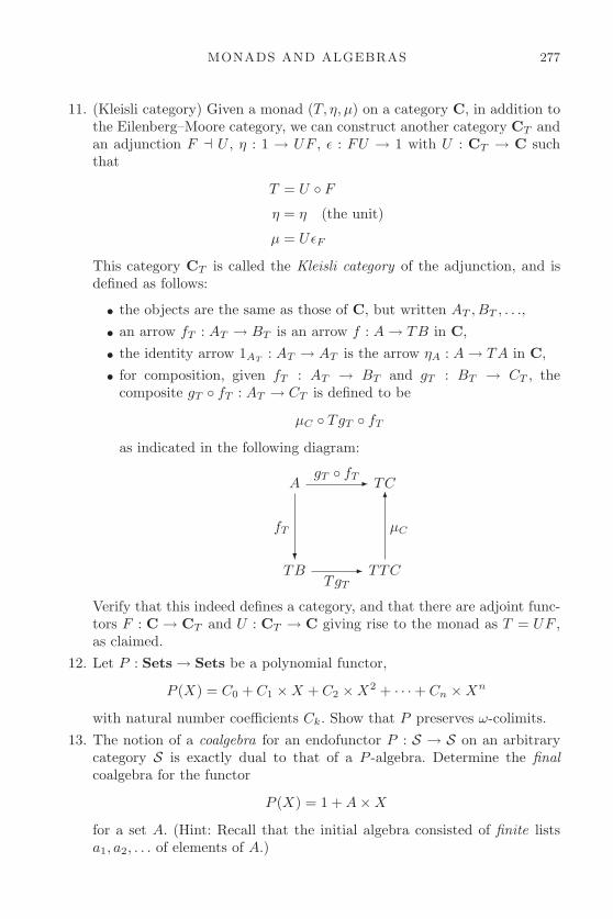
MONADS AND ALGEBRAS 277
11. (Kleisli category) Given a monad (T, η, μ) on a category C, in addition tothe Eilenberg–Moore category, we can construct another category CT andan adjunction F ! U , η : 1 → UF , ε : FU → 1 with U : CT → C suchthat
T = U ◦ F
η = η (the unit)
μ = UεF
This category CT is called the Kleisli category of the adjunction, and isdefined as follows:
• the objects are the same as those of C, but written AT , BT , . . .,
• an arrow fT : AT → BT is an arrow f : A → TB in C,
• the identity arrow 1AT: AT → AT is the arrow ηA : A → TA in C,
• for composition, given fT : AT → BT and gT : BT → CT , thecomposite gT ◦ fT : AT → CT is defined to be
μC ◦ TgT ◦ fT
as indicated in the following diagram:
AgT ◦ fT� TC
TB
fT
�
TgT
� TTC
μC
�
Verify that this indeed defines a category, and that there are adjoint func-tors F : C → CT and U : CT → C giving rise to the monad as T = UF ,as claimed.
12. Let P : Sets → Sets be a polynomial functor,
P (X) = C0 + C1 ×X + C2 ×X2 + · · ·+ Cn ×Xn
with natural number coefficients Ck. Show that P preserves ω-colimits.13. The notion of a coalgebra for an endofunctor P : S → S on an arbitrary
category S is exactly dual to that of a P -algebra. Determine the finalcoalgebra for the functor
P (X) = 1 + A×X
for a set A. (Hint: Recall that the initial algebra consisted of finite listsa1, a2, . . . of elements of A.)

This page intentionally left blank

SOLUTIONS TO SELECTED EXERCISES
Chapter 1
1. (a) Identity arrows behave correctly, for if f ⊂ A×B, then
f ◦ 1A = {〈a, b〉 | ∃a′ ∈ A : 〈a, a′〉 ∈ 1A ∧ 〈a′, b〉 ∈ f}= {〈a, b〉 | ∃a′ ∈ A : a = a′ ∧ 〈a′, b〉 ∈ f}= {〈a, b〉 | 〈a, b〉 ∈ f} = f
and symmetrically 1B ◦ f = f . Composition is associative; if f ⊆ A × B,g ⊆ B × C, and h ⊆ C ×D, then
(h ◦ g) ◦ f = {〈a, d〉 | ∃b : 〈a, b〉 ∈ f ∧ 〈b, d〉 ∈ h ◦ g}= {〈a, d〉 | ∃b : 〈a, b〉 ∈ f ∧ 〈b, d〉 ∈ {〈b, d〉 | ∃c : 〈b, c〉 ∈ g ∧ 〈c, d〉 ∈ h}}= {〈a, d〉 | ∃b : 〈a, b〉 ∈ f ∧ ∃c : 〈b, c〉 ∈ g ∧ 〈c, d〉 ∈ h}= {〈a, d〉 | ∃b∃c : 〈a, b〉 ∈ f ∧ 〈b, c〉 ∈ g ∧ 〈c, d〉 ∈ h}= {〈a, d〉 | ∃c : (∃b : 〈a, b〉 ∈ f ∧ 〈b, c〉 ∈ g) ∧ 〈c, d〉 ∈ h}= {〈a, d〉 | ∃c : 〈a, b〉 ∈ g ◦ f ∧ 〈c, d〉 ∈ h}= h ◦ (g ◦ f).
2. (a) Rel ∼= Relop. The isomorphism functor (in both directions) takes anobject A to itself, and takes a relation f ⊆ A×B to the opposite relationfop ⊆ B × A defined by fop := {〈b, a〉 | 〈a, b〉 ∈ f}. It is straightforwardto check that this is a functor Rel → Relop and Relop → Rel, and it isits own inverse.
(b) Sets �∼= Setsop. Consider maps into the empty set ∅; there is exactly one.If Sets ∼= Setsop held, there would have to be a corresponding set ∅′ withexactly one arrow out of it.
(c) P (X) ∼= P (X)op. The isomorphism takes each element U of the powersetto its complement X −U . Functoriality amounts to the fact that U ⊆ Vimplies X − V ⊆ X − U .
3. (a) A bijection f from a set A to a set B, and its inverse f−1, comprise anisomorphism; f(f−1(b)) = b and f−1(f(a)) = a, and so f ◦f−1 = 1B andf−1 ◦ f = 1A, by definition of the inverse. If an arrow f : A → B in Setsis an isomorphism, then there is an arrow g : B → A such that f ◦g = 1B
and g ◦ f = 1A. The arrow f is an injection because f(a) = f(a′) impliesa = g(f(a)) = g(f(a′)) = a′, and f is surjective because every b ∈ B hasa preimage, namely g(b), since f(g(b)) = b.

280 SOLUTIONS TO SELECTED EXERCISES
(b) Monoid homomorphisms that are isomorphisms are also isomorphisms inSets, so by the previous solution they are bijective homomorphisms. Itremains to show that bijective homomorphisms are isomorphisms. It issufficient to show that the inverse mapping of a bijective homomorphismf : M → N is a homomorphism. But we have
f−1(b �N b′) = f−1(f(f−1(b)) �N f(f−1(b′)))
= f−1(f(f−1(b) �M f−1(b′)))
= f−1(b) �M f−1(b′)
and f−1(eN ) = f−1(f(eM )) = eM .(c) Consider the posets A = (U,≤A) and B = (U,≤B) given by U = {0, 1},
≤A= {〈0, 0〉, 〈1, 1〉}, and ≤B= {〈0, 0〉, 〈0, 1〉, 〈1, 1〉}. The identity functioni : U → U is an arrow A → B in Posets, and it is a bijection, but theonly arrows B → A in Posets are the two constant functions U → U ,because arrows in Posets must be monotone. Neither is an inverse to i,which is therefore not an isomorphism.
6. The coslice category C/C, the category whose objects are arrows f : C → Afor A ∈ C and whose arrows f → f ′ are arrows h completing commutativetriangles
A
Cf ′
�
f
�
B
h
�
can equivalently be described as (Cop/C)op. For example, in the above dia-gram f, f ′ are arrows into C in the opposite category Cop, so they are objectsin the slice Cop/C. The arrow h is B → A in Cop and h ◦ f = f ′ so it is anarrow B → A in Cop/C, hence an arrow A → B in (Cop/C)op.
9. The free category on the graph
•
•h
�
f
�
•
g
�

SOLUTIONS TO SELECTED EXERCISES 281
is•
•h �
gf�
f
�
•
g
�
plus three identity arrows, one for each object. The free category on the graph
•f ��g
•
has infinitely many arrows, all possible finite sequence of alternating fs andgs—there are two empty sequences (i.e., identity arrows), one for each object.
10. The graphs whose free categories have exactly six arrows are the discretegraph with six nodes, and the following 10 graphs:
• • • • •
• • • • •
• • • •
• • • • • •
• • • • • •
•• • •
•••••

282 SOLUTIONS TO SELECTED EXERCISES
11. (a) The functor M : Sets → Mon that takes a set X to the free monoid onX (i.e., strings over X and concatenation) and takes a function f : X → Yto the function M(f) defined by M(f)(a1 . . . ak) = f(a1) . . . f(ak) is a func-tor; M(f) is a monoid homomorphism MX → MY since it preserves themonoid identity (the empty string) and the monoid operation (composi-tion). It can be checked that M preserves identity functions and composition:M(1X)(a1 . . . ak) = 1X(a1) . . . 1X(ak) = a1 . . . ak and
M(g ◦ f)(a1 . . . ak) = (g ◦ f)(a1) . . . (g ◦ f)(ak)
= g(f(a1)) . . . g(f(ak)) = M(g)(M(f)(a1 . . . ak))
= (M(g) ◦M(f))(a1 . . . ak).
12. Let D be a category and h : G → U(D) be a graph homomorphism. Supposeh is a functor C(G) → D such that
U(h) ◦ i = h (∗).
From this equation, we see that U(h)(i(x)) = h(x) for all vertices andedges x ∈ G. So the behavior of h on objects and paths of length one(i.e., arrows in the image of i) in C(G) is completely determined by therequirement (∗). But since h is assumed to be a functor, and so must pre-serve composition, its behavior on arrows in C(G) that correspond to longerpaths in G is also determined, by a simple induction. Now it must be thath(f1 · · · fk) = h(f1) ◦ · · ·h(fk) if h is a functor, and similarly h(εA) = 1A,where εA is the empty path at A. So uniqueness of h is established, andit is easily checked that this definition is indeed a functor, so the UMP issatisfied.
Chapter 2
1. Suppose f : A → B is epi and not surjective. Choose b ∈ B not in the rangeof f . Define g1, g2 : B → {0, 1} as follows: g1(x) = 0 for all x ∈ B, andg2(x) = 1 if x = b, and 0 otherwise. Note that g1 ◦ f = g2 ◦ f by choiceof b, a contradiction. In the other direction, suppose f is surjective, andsuppose g1, g2 : B → C are such that g1 �= g2. Then there is b ∈ B suchthat g1(b) �= g2(b). By assumption, b has a preimage a such that f(a) = b.So g1(f(a)) �= g2(f(a)) and g1 ◦ f �= g2 ◦ f .
4. (a) Iso: the inverse of h is f−1 ◦g−1. Monic: If h◦k1 = h◦k2, then g◦ f◦k1 =g ◦ f ◦ k2. Since g is monic, f ◦ k1 = f ◦ k2. Since f is monic, k1 = k2. Epi:dual argument.
(b) If f ◦ k1 = f ◦ k2, then g ◦ f ◦ k1 = g ◦ f ◦ k2. Since h is monic, k1 = k2.(c) Dual argument to (b).(d) In Sets, put A = C = {0}, B = {0, 1}, and all arrows constantly 0. h is
monic but g is not.

SOLUTIONS TO SELECTED EXERCISES 283
5. Suppose f : A → B is an isomorphism. Then f is mono because f ◦k1 = f ◦k2
implies k1 = f−1 ◦ f ◦ k1 = f−1 ◦ f ◦ k2 = k2, and dually f is mono also.Trivially, f is split mono and split epi because f ◦f−1 = 1B and f−1◦f = 1A.So we know (a)⇒(b), (c), (d). If f is mono and split epi, then there is g suchthat f◦g = 1B . But since f is mono, (f◦g)◦f = f◦(g◦f) = f = f◦1A impliesg ◦ f = 1A and so g is in fact the inverse of f , and we have (b)⇒(a). Dually,(c)⇒(a). The fact that (d)⇒(b), (c) needs only that split mono implies mono(or dually that split epi implies epi). If there is g such that g ◦ f = 1A, thenf ◦ k1 = f ◦ k2 implies k1 = g ◦ f ◦ k1 = g ◦ f ◦ k2 = k2.
6. If h : G → H is injective on edges and vertices, and h ◦ f = h ◦ g in Graphs,then the underlying set functions on edges and vertices are mono arrows inSets, so the edge and vertex parts of f and g are equal, and so f = g. Ifh : G → H is mono in Graphs, and it is not injective on vertices, thenthere are two vertices v, w such that h(v) = h(w). Let 1 be the graph withone vertex, and f, g be graph homomorphisms 1 → G taking that vertexto v, w, respectively. Then, h ◦ f = h ◦ g. A similar argument holds foredges.
9. First, in the category Pos, an arrow is epi iff it is surjective: suppose thatf : A → B is surjective and let g, h : B → C with gf = hf . In Pos, thismeans that g and h agree on the image of f , which by surjectivity is all of B.Hence g = h and f is epi. On the other hand, suppose f is not epi and thatg, h : B → C witness this. Since g �= h, there is some b ∈ B with g(b) �= h(b).But from this b �∈ f(A), and so A is not surjective.Next, the singleton set 1, regarded as a poset, is projective: suppose f : 1 →Y and e : X � Y are arrows in Pos, with e epi. Then e is surjective, so thereis some x ∈ X with e(x) = f(∗). Any map ∗ �→ x witnesses the projectivityof 1.
10. Any set A is projective in Pos: suppose that f : A → Y and e : X � Y arearrows in Pos. Choose for each y ∈ Y an element xy ∈ X with f(xy) = y; thisis possible since e is epi and hence surjective. Now define a map f : A → Xby a �→ xf(a). Since A is discrete this is necessarily monotonic, and we haveef = f , so A is projective.For contrast, the two element poset P = {0 ≤ 1} is not projective. Indeed,we may take f to be the identity and X to be the discrete two-element set{a, b}. Then the surjective map e : a �→ 0, b �→ 1 is an epi, since it is surjective.However, any monotone map g : P → {a, b} must identify 0 and 1, since theonly arrows in the second category are identities. But then e ◦ g �= 1P . Thus,there is no function g lifting the identity map on P across e, so P is notprojective.Moreover, every projective object in Pos is discrete: For suppose Q is projec-tive. We can always consider the discretation |Q| of Q, which has the sameobjects as Q and only identity arrows. We clearly get a map |Q| → Q which

284 SOLUTIONS TO SELECTED EXERCISES
is surjective and hence epi. This means that we can complete the diagram
|Q|
Q1Q
�
f
�
Q
|1Q|
�
But the only object function that could possibly commute in this situationis the object identity. Then,
x ≤ x′ ⇐⇒ f(x) ≤ f(x′) ⇐⇒ f(x) = f(x′) ⇐⇒ x = x′.
But then the only arrows of Q are identity arrows, so Q is discrete, as claimed.Thus, the projective posets are exactly the discrete sets. Clearly, compositionof maps and identity arrows of discrete posets are exactly those of Set, soSet is a subcategory of Pos. Moreover, every function between discrete setsis monotone, so this is a full subcategory.
11. The UMP of a free monoid states that for any f : A → UB, there is a uniquef : MA → B such that
UMAUf� UB
(∗)
A
η
�
f
�
commutes. For η : A → UM to be an initial object in A-Mon, it must bethat for object f : A → UB, there is a unique arrow f in A-Mon from ηto f . But the definition of arrow in A-Mon is such that this arrow mustcomplete exactly the commutative triangle (∗) above. Therefore, the twocharacterizations of the free monoid coincide.
13. Let P be the iterated product A×(B×C) with the obvious maps p1 : P → A,p2 : P → B×C → B, and p3 : P → B×C → C. Define Q = (A×B)×C andqi similarly. By the UMP, we get a unique map f1 = p1 × p2 : P → A × B.Applying it again, we get a unique map f = (p1 × p2) × p3 : P → Q withqif = pi. We can run a similar argument to get a map g in the other direction.Composing, we get gf : P → P which respects the pi. By the UMP, such amap is unique, but the identity is another such map. Thus they must be thesame, so gf = 1P . Similarly fg = 1Q, so f and g are inverse and P ∼= Q.
17. The pairing of any arrow with the identity is in fact split mono: π1◦〈1A, f〉 =1A. There is a functor G : Sets → Rel which is constant on objects andtakes f : A → B to (im 〈1A, f〉) ⊆ A × B. It preserves identities since

SOLUTIONS TO SELECTED EXERCISES 285
G(1A) im 〈1A, 1A〉 = {〈a, a〉 | a ∈ A} = 1A ∈ Rel. It preserves compositionbecause for g : B → C, we have
G(g ◦ f) = im 〈1A, g ◦ f〉 = {〈a, g(f(a))〉 | a ∈ A}
= {〈a, c〉 | ∃b ∈ B.b = f(a) ∧ c = g(b)}
= {〈b, g(b)〉 | b ∈ B} ◦ {〈a, f(a)〉 | a ∈ A}
= G(g) ◦G(f).
Chapter 3
1. In any category C, the diagram
A �c1
Cc2
� B
is a product diagram iff the mapping
hom(Z,C) −→ hom(Z,A)× hom(Z,B)
given by f �→ 〈c1 ◦ f, c2 ◦ f〉 is an isomorphism. Applying this fact to Cop,the claim follows.
2. Say iMA, iMB are the injections into the coproduct MA+MB, and ηA, ηB arethe injections into the free monoids on A,B. Put e = [U(iMA)◦ηA, U(iMB)◦ηB ]. Let an object Z and an arrow f : A + B → UZ be given. Supposeh : MA + MB → Z has the property that
Uh ◦ e = f (∗)
Because of the UMP of the coproduct, we have generally that a ◦ [b, c] =[a ◦ b, a ◦ c], and in particular
Uh ◦ e = [Uh ◦ U(iMA) ◦ ηA, Uh ◦ U(iMB) ◦ ηB ]
Because this is equal to f , which is an arrow out of A+B, and since functorspreserve composition, we have
U(h ◦ iMA) ◦ ηA = f ◦ iA
U(h ◦ iMB) ◦ ηB = f ◦ iB
where iA, iB are the injections into A + B. But the UMP of the free monoidimplies that h ◦ iMA must coincide with the unique f ◦ iA that makes the

286 SOLUTIONS TO SELECTED EXERCISES
triangle
MA ....................f ◦ iA� Z
UMA ................Uf ◦ iA� UZ
A
ηA
�
f ◦ iA
�
commute. Similarly, h ◦ iMB = f ◦ iB . Since its behavior is known onboth injections, h is uniquely determined by the condition (∗); in fact,h = [f ◦ iA, f ◦ iB ]. That is, the UMP of the free monoid on A+B is satisfiedby MA+MB. Objects characterized by UMPs are unique up to isomorphism,so M(A + B) ∼= MA + MB.
5. In the category of proofs, we want to see that (modulo some identifications)the coproduct of formulas ϕ and ψ is given by ϕ ∨ ψ. The intro and elimrules automatically give us maps (proofs) of the coproduct from either ofits disjuncts, and from pairs of proofs that begin with each of the disjunctsinto a single proof beginning with the disjunction. To see that this objectreally is a coproduct, we must verify that this is the unique commutingarrow.
ϕi � ϕ ∨ ψ � j
ψ
θ
[p, q]
�q
�
p�
But this is simple since composition is simply concatenation of proofs. Sup-pose we have another proof r : ϕ∨ψ → θ with r ◦ i = p. Then by disjunctionelimination, r necessarily has the form
ϕ ∨ ψ
[ϕ]....θ
[ψ]....θ
θ .
Applying i on the right simply has the effect of bringing down part of the
proof above, so that the quotienting equation now reads r◦i =
[ϕ]....θ = p. Hence,
up to the presence of more detours, we know that the proof appearing as part

SOLUTIONS TO SELECTED EXERCISES 287
of r is exactly p. Similarly, we know that the second part of the proof
[ψ]....θ
must be q. Thus r is uniquely defined (up to detours) by p and q, ϕ ∨ ψ isindeed a coproduct.
6. (Equalizers in Ab). Suppose we have a diagram
(A,+A, 0A)f�
g� (B,+B , 0B)
in Ab. Put A′ := {a ∈ A | f(a) = g(a)}. It is easy to check that A′ is in facta subgroup of A, so it remains to be shown that
(A′,+A, 0A) ⊂� (A,+A, 0A)f�
g� (B,+B , 0B)
is an equalizer diagram.
(X, +X , 0X)
(A′,+A, 0A)
h
�⊂� (A,+A, 0A)
f�
g�
z
�
(B,+B , 0B)
If the triangle is to commute, h(x) = z(x) for all x ∈ X, so h is uniquelydetermined. It is easily checked that h is a homomorphism, implying thatAb indeed has all equalizers.
14. (a) The equalizer of f ◦ π1 and f ◦ π2 is the relation ker(f) = {〈a, a′〉 ∈A × A | f(a) = f(a′)}. Symmetry, transitivity, and reflexivity of ker(f)follow immediately from the same properties of equality.
(b) We need to show that a pair a, a′ of elements are in the kernel of theprojection q : A �� A/R iff they are related by R. But this amountsto saying that q(a) = q(a′) iff aRa′, where q(x) = {x | xRa} is theequivalence class. But this is true since R is an equivalence relation.
(c) Take any function f : A → B with f(a) = f(a′) for all aRa′. The kernelker(f) of f is therefore an equivalence relation that contains R, so 〈R〉 ⊆ker(f). It follows that f factors through the projection q : A �� A/〈R〉(necessarily uniquely, since q is epic).
(d) The coequalizer of the projections from R is the projection q :A �� A/〈R〉, which has 〈R〉 as its kernel.

288 SOLUTIONS TO SELECTED EXERCISES
Chapter 4
1. Given a categorical congruence ∼ on a group G, the corresponding normalsubgroup is N∼ := {g | g ∼ e}. N is a subgroup; it contains the identityby reflexivity of ∼. It is closed under inverse by symmetry and the fact thate ∼ g implies g−1 = g−1e ∼ g−1g = e. It is closed under product because ifg ∼ e and h ∼ e then gh ∼ ge = g ∼ e, and by transitivity gh ∈ N∼. It isnormal because
x{g | g ∼ e} = {xg | g ∼ e} = {x(x−1h) | x−1h ∼ e} = {h | h ∼ x}and
{g | g ∼ e}x = {gx | g ∼ e} = {(hx−1)x | hx−1 ∼ e} = {h | h ∼ x}.In the other direction, the categorical congruence ∼N corresponding to anormal subgroup N is g ∼N h : ⇐⇒ gh−1 ∈ N . The fact that ∼N is anequivalence follows easily from the fact that N is a subgroup. If f ∼N g, thenalso hfk ∼N hgk, since fg−1 ∈ N implies hfkk−1g−1h−1 = hfg−1h−1 ∈ N ,because N was assumed normal, and so N = hNh−1.Since two elements g, h of a group are in the same coset of N precisely whengh−1 = e, the quotient G/N and the quotient G/∼ coincide when N and ∼are in the correspondence described above.
6. (a)
1 � 2 � 3
No equations. (i.e., 3 is free)(b)
1f �
g� 2 � 3
Equations: f = g
(c)
1f �
g� 2
h �
k� 3
Equations: f = g, h = k
(d)
1f � 2
2
h
�
g�

SOLUTIONS TO SELECTED EXERCISES 289
Equations: f = h ◦ g
7. By definition of congruence, f ∼ f ′ implies gf ∼ gf ′ and g ∼ g′ impliesgf ′ ∼ g′f ′. By transitivity of ∼, we conclude gf ∼ g′f ′.
8. ∼ is an equivalence because equality is. For instance, if f ∼ g, then for allE and H : D → E we have HF = HG ⇒ H(f) = H(g). But under thesame conditions, we have H(g) = H(f), so g ∼ f . Since H is assumed tobe a functor, it preserves composition, and so H(hfk) = H(h)H(f)H(k) =H(h)H(g)H(k) = H(hgk) for any H such that HF = HG and any h, k,hence ∼ is a congruence.Let q be the functor assigning all the arrows in D to their ∼-equivalenceclasses in the quotient D/∼. We know q is indeed a well-defined functor bya previous exercise. Suppose we have H coequalizing F,G. By definitionof ∼ any arrows that H identifies are ∼-equivalent, and therefore iden-tified also by q. There can be at most one K making the trianglein
CF �
G� D
q � D/∼
E
H
�K
�
commute, (for any [f ]∼ ∈ D/∼ it must be that K([f ]∼) =H(f)) and the fact that q identifies at least as many arrows as Himplies the existence of such a K. So q is indeed the coequalizer ofF,G.
Chapter 5
1. Their UMPs coincide. A product in C/X of f and g is an object h : A ×X
B → X and projections π1 : h → f and π2 : h → g which is terminalamong such structures. The pullback of f, g requires an object A×X B andprojections π1 : A ×X B → A and π2 : A ×X B → B such that f ◦ π1 =g ◦ π2, terminal among such structures. The commutativity requirements ofthe pullback are exactly those imposed by the definition of arrow in the slicecategory.
2. (a) If m is monic, then the diagram is a pullback; if m ◦ f = m ◦ g, thenf = g, the unique mediating map being equivalently f or g. If the diagramis a pullback, suppose m ◦ f = m ◦ g. The definition of pullback implies theunique existence of h such that 1M ◦ h = f and 1M ◦ h = g, but this impliesf = g.

290 SOLUTIONS TO SELECTED EXERCISES
3.
Zh �
k� M ′ f ′
� M
A′
m′
�
f� A
m
�
Let h, k : Z → M ′ be given. Suppose m′h = m′k. Then, fm′h = fm′k andso mf ′h = mf ′k. Since m is assumed mono, f ′h = f ′k. The definition ofpullback applied to the pair of arrows m′k, f ′k implies, there is exactly onearrow q : Z → M ′ such that m′ ◦ q = m′k and f ′ ◦ q = f ′k. But both h, kcan be substituted for q and satisfy this equation, so h = k.
4. Suppose m : M → A and n : N → A are subobjects of A. If M ⊆ N , thenthere is an arrow s : M → N such that n ◦ s = m. If z ∈A M , then there isan arrow f : Z → M such that m◦f = z. Then s◦f witnesses z ∈A N , sincen ◦ s ◦ f = m ◦ f = z. If for all z : Z → A we have z ∈A M⇒z ∈A N , thenin particular this holds for z = m, and in fact m ∈A M (via setting f = 1A)so m ∈A N , in other words M ⊆ N .
7. We show that the representable functor HomC(C,−) : C → Sets preservesall small products and equalizers; it follows that it preserves all small limits,since the latter can be constructed from the former. For products, we needto show that for any set I and family (Di)i∈I of objects of C, there is a(canonical) isomorphism,
Hom(C,∏i∈I
Di) ∼=∏i∈I
Hom(C,Di).
But this follows immediately from the definition of the product∏
i∈I Di.For equalizers, consider an equalizer in C,
Ee � A
f �
g� B.
Applying Hom(C,−) results in the following diagram in Sets:
Hom(C,E)e∗ � Hom(C,A)
f∗ �
g∗� Hom(C,B),
which is clearly an equalizer: for, given h : C → A with f∗(h) = g∗(h), wetherefore have fh = f∗(h) = g∗(h) = gh, whence there is a unique u : C → Ewith h = eu = e∗(u).
8. We have a putative category of partial maps. We need to verify identity andassociativity. The first is easy. Any object is a subobject of itself, so we may

SOLUTIONS TO SELECTED EXERCISES 291
set 1A in the category of partial maps to be the pair (1A, A). It is trivial tocheck that this acts as an identity.For associativity, suppose U , V , and W are subobjects of A, B, and C,respectively, and that we have maps as in the diagram:
U ×B V V ×C W
U�
⊃
V
�
⊃�
W
�
A
�
⊃
B�
⊃f�
C
�
⊃g�
D
h�
Now let P be the pullback of U×BV and V ×C W over E and k the associatedpartial map. Since we can compose pullback squares, that means that P isalso the pullback of U and V ×C W over B. Since the latter is the compositionof g and h, this means k = (h ◦ g) ◦ f . Similarly, k = h ◦ (g ◦ f). Hence thecomposition of partial maps is associative, and this setup does describe acategory.
12. If we let the numeral n denote the initial segment of the natural numbersequence {0 ≤ 1 ≤ . . . ≤ n}, we have a chain of inclusions in Pos:
0 → 1 → 2 → . . . → n → . . . .
We would like to determine the limit and colimit of the diagram.For the limit, suppose we have a cone ζn : Z → n. Since 0 is the initial object,ζ0 is constant, and each map ζn has ζ0 as a factor (this is the cone condition).But each such map simply takes 0 to itself, regarded as an element of n, sothat ζn is also the constant zero map. So the limit of the diagram can be(anything isomorphic to) the object 0 together with the inclusions 0 → n.Now suppose we have a co-cone ψn : n → Y . The co-cone condition impliesthat ψn is simply the restriction of ψm+n to the subset n ⊆ n+m. If m < n,then
ψ(m) = ψm(m) = ψn(m) < ψn(n)
so this is a monotone function. For any other ϕ : N → Y , there is some nwith ϕ(n) �= ψ(n) = ψn(n). Thus, ψ is the unique map factoring the co-coneon Y . Thus, ω = {0 ≤ 1 ≤ 2 ≤ . . .} together with the evident injectionsn → ω is the colimit of the diagram.
Chapter 6
Notation: If f : A → BC , then ev ◦ f × C = f : A× C → B. If f : A× C → B,then λf : A → BC .
2. These isomorphism are witnessed by the following pairs: f : (A × B)C →AC × BC defined by f = 〈λ(π1 ◦ 1(A×B)C ), λ(π2 ◦ 1(A×B)C )〉 and f−1 :AC × BC → (A× B)C defined by f−1 = λ〈π1, π2〉; and g : (AB)C → AB×C

292 SOLUTIONS TO SELECTED EXERCISES
defined by g = λ(ev ◦ α(AB)C ) and g−1 : AB×C → (AB)C defined byg−1 = λλ(ev ◦ α−1
AB×C ), where αZ is the evident isomorphism from associati-vity and commutativity of the product, up to isomorphism, Z × (B × C) →(Z × C)×B.
3. The exponential transpose of ev is 1BA . The exponential transpose of 1A×B
is the “partial pairing function” A → (A×B)B defined by a �→ λb : B.〈a, b〉.The exponential transpose of ev ◦ τ is the “partial application function”A → BBA
defined by a �→ λf : BA.f(a).6. Here we consider the category Sub, whose objects are pairs (A,P ⊆ A), and
whose arrows f : (A,P ) → (B,Q) are set functions A → B such that a ∈ Piff f(a) ∈ Q. This means that an arrow in this category is essentially a pairof arrows f1 : P → Q and f2 : A \ P → B \ Q; thus, this is (isomorphic to)the category Sets/2.Now, Sets/2 is equivalent to the product category Sets×Sets, by a previousexercise. This latter category is cartesian closed, by the equational definitionof CCCs, which clearly holds in the two factors. But equivalence of categoriespreserves cartesian closure, so Sub is also cartesian closed.
10. For products, check that the set of pairs of elements of ωCPOs A and Bordered pointwise, constitutes an ωCPO (with ω-limits computed pointwise)and satisfies the UMP of a product. Similarly, the exponential is the setof continuous monotone functions between A and B ordered pointwise, withlimits computed pointwise. In strict ωCPOs, by contrast, there is exactly onemap {⊥} → A, for any object A. Since {⊥} = 1 is also a terminal object,however, given an exponential BA there can be only one map A → B, sinceHom(A,B) ∼= Hom(1×A,B) ∼= Hom(1, BA).
11. (a) The identity((p ∨ q) ⇒ r) ⇒ ((p ⇒ r) ∧ (q ⇒ r))
“holds” in any CC poset with joins, that is, this object is equal to thetop element 1. Equivalently, from the definition of ⇒, we have
((p ∨ q) ⇒ r) ≤ ((p ⇒ r) ∧ (q ⇒ r)),
as follows immediately from part (b), which shows the existence of suchan arrow in any CCC.
(b) In any category where the constructions make sense, there is an arrow
C(A+B) → CA × CB .
Indeed, by the definition of the coproduct, we have arrows A → A + Band B → A + B, to which we apply the contravariant functor C(−) toobtain maps C(A+B) → AC and C(A+B) → CB . By the UMP of theproduct, this gives a map C(A+B) → CA × CB , as desired.
13. This can be done directly by comparing UMPs. For a different proof (antici-pating the Yoneda lemma), consider, for an arbitrary object X, the bijective
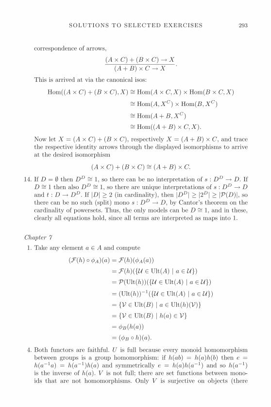
SOLUTIONS TO SELECTED EXERCISES 293
correspondence of arrows,
(A× C) + (B × C) → X
(A + B)× C → X.
This is arrived at via the canonical isos:
Hom((A× C) + (B × C), X) ∼= Hom(A× C,X)×Hom(B × C,X)
∼= Hom(A,XC)×Hom(B,XC)
∼= Hom(A + B,XC)∼= Hom((A + B)× C,X).
Now let X = (A× C) + (B × C), respectively X = (A + B)× C, and tracethe respective identity arrows through the displayed isomorphisms to arriveat the desired isomorphism
(A× C) + (B × C) ∼= (A + B)× C.
14. If D = ∅ then DD ∼= 1, so there can be no interpretation of s : DD → D. IfD ∼= 1 then also DD ∼= 1, so there are unique interpretations of s : DD → Dand t : D → DD. If |D| ≥ 2 (in cardinality), then |DD| ≥ |2D| ≥ |P(D)|, sothere can be no such (split) mono s : DD → D, by Cantor’s theorem on thecardinality of powersets. Thus, the only models can be D ∼= 1, and in these,clearly all equations hold, since all terms are interpreted as maps into 1.
Chapter 7
1. Take any element a ∈ A and compute
(F(h) ◦ φA)(a) = F(h)(φA(a))
= F(h)({U ∈ Ult(A) | a ∈ U})= P(Ult(h))({U ∈ Ult(A) | a ∈ U})= (Ult(h))−1({U ∈ Ult(A) | a ∈ U})= {V ∈ Ult(B) | a ∈ Ult(h)(V)}= {V ∈ Ult(B) | h(a) ∈ V}= φB(h(a))
= (φB ◦ h)(a).
4. Both functors are faithful. U is full because every monoid homomorphismbetween groups is a group homomorphism: if h(ab) = h(a)h(b) then e =h(a−1a) = h(a−1)h(a) and symmetrically e = h(a)h(a−1) and so h(a−1)is the inverse of h(a). V is not full; there are set functions between mono-ids that are not homomorphisms. Only V is surjective on objects (there
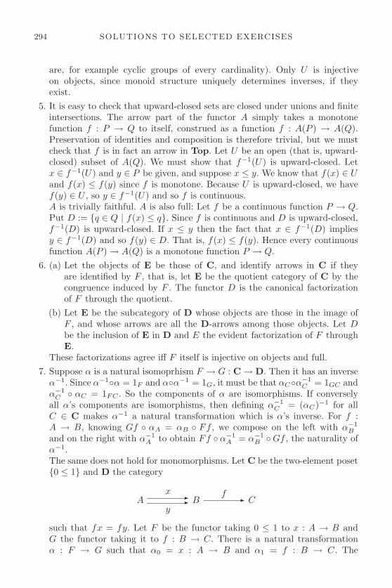
294 SOLUTIONS TO SELECTED EXERCISES
are, for example cyclic groups of every cardinality). Only U is injectiveon objects, since monoid structure uniquely determines inverses, if theyexist.
5. It is easy to check that upward-closed sets are closed under unions and finiteintersections. The arrow part of the functor A simply takes a monotonefunction f : P → Q to itself, construed as a function f : A(P ) → A(Q).Preservation of identities and composition is therefore trivial, but we mustcheck that f is in fact an arrow in Top. Let U be an open (that is, upward-closed) subset of A(Q). We must show that f−1(U) is upward-closed. Letx ∈ f−1(U) and y ∈ P be given, and suppose x ≤ y. We know that f(x) ∈ Uand f(x) ≤ f(y) since f is monotone. Because U is upward-closed, we havef(y) ∈ U , so y ∈ f−1(U) and so f is continuous.A is trivially faithful. A is also full: Let f be a continuous function P → Q.Put D := {q ∈ Q | f(x) ≤ q}. Since f is continuous and D is upward-closed,f−1(D) is upward-closed. If x ≤ y then the fact that x ∈ f−1(D) impliesy ∈ f−1(D) and so f(y) ∈ D. That is, f(x) ≤ f(y). Hence every continuousfunction A(P ) → A(Q) is a monotone function P → Q.
6. (a) Let the objects of E be those of C, and identify arrows in C if theyare identified by F , that is, let E be the quotient category of C by thecongruence induced by F . The functor D is the canonical factorizationof F through the quotient.
(b) Let E be the subcategory of D whose objects are those in the image ofF , and whose arrows are all the D-arrows among those objects. Let Dbe the inclusion of E in D and E the evident factorization of F throughE.
These factorizations agree iff F itself is injective on objects and full.7. Suppose α is a natural isomoprhism F → G : C → D. Then it has an inverse
α−1. Since α−1◦α = 1F and α◦α−1 = 1G, it must be that αC◦α−1C = 1GC and
α−1C ◦ αC = 1FC . So the components of α are isomorphisms. If conversely
all α’s components are isomorphisms, then defining α−1C = (αC)−1 for all
C ∈ C makes α−1 a natural transformation which is α’s inverse. For f :A → B, knowing Gf ◦ αA = αB ◦ Ff , we compose on the left with α−1
B
and on the right with α−1A to obtain Ff ◦ α−1
A = α−1B ◦Gf , the naturality of
α−1.The same does not hold for monomorphisms. Let C be the two-element poset{0 ≤ 1} and D the category
Ax �
y� B
f � C
such that fx = fy. Let F be the functor taking 0 ≤ 1 to x : A → B andG the functor taking it to f : B → C. There is a natural transformationα : F → G such that α0 = x : A → B and α1 = f : B → C. The

SOLUTIONS TO SELECTED EXERCISES 295
component f of α is not mono, but α itself is; there are no nontrivial naturaltransformations into F : any β : H → F would have to satisfy a naturalitysquare
H0H ≤� H1
A
β0
�
x� B
β1
�
But H0 must be A and β0 = 1A. Then H1 must be either A or B, forcingβ to either be the unique natural transformation to F from the functortaking 0 ≤ 1 to 1A : A → A, or else the identity natural transformationon F .
8. Put (F ×G)(C) = FC ×GC, and (F ×G)(f) = Ff ×Gf . Define (π1)C =πFC×GC
1 : FC × GC → FC and (π2)C = πFC×GC2 : FC × GC → GC.
It is easy to check that π1, and π2 are natural. Let a functor Z : C → Dand natural transformations α : Z → F and β → F be given. By the UMPof the product, there are unique arrows hC : ZC → FC × GC such that(π1)C ◦ hC = αC and (π2)C ◦ hC = βC . We need to verify that
ZChC� FC ×GC
ZD
Zf
�
hD
� FD ×GD
Ff ×Gf
�
ButπFD×GD
1 ◦ Ff ×Gf ◦ hC = Ff ◦ πFC×GC1 ◦ hC
= Ff ◦ αC = αD ◦ Zf = πFD×GD1 ◦ hD ◦ Zf.
And similarly with the second projection, using the naturality of β.10. To satisfy the bifunctor lemma, we need to show that for any f : C → C ′ ∈
Cop and g : D → D′ ∈ C the following commutes:
hom(C,D)hom(f,D)� hom(C ′, D)
hom(C,D′)
hom(C, g)
�
hom(f,D′)� hom(C ′, D′)
hom(C ′, g)
�

296 SOLUTIONS TO SELECTED EXERCISES
But either path around the square takes an arrow h : C → D and turns itinto g ◦ h ◦ f : C ′ → D′; thus the associativity of composition implies thatthe square commutes.
12. If C # D, then there are functors F : C � D : G and natural isomorphismsα : 1D → FG and β : GF → 1C. Suppose C has products, and let D,D′ ∈ Dbe given. We claim that F (GD × GD′) is a product object of D and D′,with projections α−1
D ◦ FπGD×GD′
1 and α−1D′ ◦ FπGD×GD′
2 . For suppose wehave an object Z and arrows a : Z → D and a′ : Z → D′ in D. Thereis a unique h : GZ → GD × GD′ ∈ C such that πGD×GD′
1 ◦ h = Ga andπGD×GD′
2 ◦ h = Ga′. Then the mediating map in D is Fh ◦ αZ . We cancalculate
α−1D ◦ FπGD×GD′
1 ◦ Fh ◦ αZ = α−1D ◦ F (πGD×GD′
1 h) ◦ αZ
= α−1D ◦ FGa ◦ αZ
= α−1D ◦ αD ◦ a
= a
and similarly for the second projection.Uniqueness of the map Fh ◦ αZ follows from that of h.
16. Let C be given. Choose one object D[C]∼= from each isomorphism class [C]∼=of objects in C and call the resulting full subcategory D. For every objectC of C choose an isomorphism iC : C → D[C]∼= . Then, C is equivalentto D via the inclusion functor I : D → C and the functor F defined byFC = D[C]∼= and F (f : A → B) = iB ◦ f ◦ i−1
A (F is a functor because theiCs are isomorphisms) and i construed as a natural isomorphism 1D → FIand 1C → IF . Naturality is easy to check:
AiA � IFA
B
f
�
iB� IFB
iBfi−1A
�
So C is equivalent to the skeletal category D.
Chapter 8
1. Let f : C � C ′ : g be an iso. Then, clearly, Ff : FC � FC ′ : Fg isalso one. Conversely, if p : FC � FC ′ : q is an iso, then since F is fullthere are f : C � C ′ : g with Ff = p and Fg = q. Then g ◦ f = 1C
since F (g ◦ f) = Fg ◦ Ff = 1FC = F (1C), and F is faithful. Similarly,f ◦ g = 1C′ .

SOLUTIONS TO SELECTED EXERCISES 297
2. Given two natural transformations ϕ,ψ : P → Q, where P,Q ∈ SetsCop
,assume that for each C ∈ C and θ : yC → P , we have ϕ ◦ θ = ψ ◦ θ. In otherwords,
ϕC∗ = ψC∗ : hom(yC, P ) → hom(yC,Q).
The Yoneda lemma gives us a bijection hom(yC, P ) ∼= PC for each C, andthese bijections are natural in P , so the following diagram commutes:
hom(yC, P )∼=� PC
hom(yC,Q)
ϕC∗ = ψC∗�
∼=� QC
ϕC
�
ψC
�
But then both ϕC and ψC must be given by the single composition throughthe left side of the square, so that ϕ = ψ.
3. The following isos are natural in Z:
homC(Z,AB ×AC) ∼= homC(Z,AB)× homC(Z,AC)∼= homC(Z ×B,A)× homC(Z × C,A)∼= homC((Z ×B) + (Z × C), A)∼= homC(Z × (B + C), A)
∼= homC(Z,AB+C).
Hence AB × AC ∼= AB+C , since the Yoneda embedding is full and faithful.The case of (A×B)C ∼= AC ×BC is similar.
6. Limits in functor categories DC can be computed “pointwise”: given F : J →DC set
(lim←−j∈J
Fj)(C) = lim←−j∈J
(Fj(C)).
Thus, it suffices to have limits in D in order to have limits in DC. Colimitsin DC are limits in (DC)op = (Dop)C
op.
7. The following are natural in C:
y(A×B)(C) ∼= hom(C,A×B)∼= hom(C,A)× hom(C,B)∼= y(A)(C)× y(B)(C)∼= (y(A)× y(B))(C),

298 SOLUTIONS TO SELECTED EXERCISES
so y(A×B) ∼= y(A)×y(B). For exponentials, take any A,B,C and compute:
y(B)y(A)(C) ∼= hom(yC, yByA)∼= hom(yC × yA, yB)∼= hom(y(C ×A), yB)∼= hom(C ×A,B)
∼= hom(C,BA)
∼= y(BA)(C).
12. (a) For any poset P, the subobject classifier Ω in SetsP is the functor:
Ω(p) = {F ⊆ P | (x ∈ F ⇒ p ≤ x) ∧ (x ∈ F ∧ x ≤ y ⇒ y ∈ F )},that is, Ω(p) is the set of all upper sets above p. The action of Ω on p ≤ qis by “restriction”: F �→ F |q = {x ∈ F | q ≤ x}. The point t : 1 → Ω isgiven by selecting the maximal upper set above p,
tp(∗) = {x | p ≤ x}.In Sets2, the subobject classifier is therefore the functor Ω : 2 → Setsdefined by
Ω(0) = {{0, 1}, {1}}Ω(1) = {{1}},
together with the natural transformation t : 1 → Ω with
t0(∗) = {0, 1}t1(∗) = {1}.
In Setsω, the subobject classifier is the functor Ω : ω → Sets defined by
Ω(0) = {{0, 1, 2, . . . }, {1, 2, 3, . . . }, {2, 3, 4, . . . }, . . . }Ω(1) = {{1, 2, 3, . . . }, {2, 3, 4, . . . }, {3, 4, 5, . . . }, . . . }
... =...
Ω(n) = {{n, n + 1, n + 2, . . . }, {n + 1, n + 2, n + 3, . . . }, . . . },with the transition maps Ω(n) → Ω(n+1) defined by taking {n, n+1, n+2, . . . } to {n + 1, n + 2, n + 3, . . . } and like sets to themselves, togetherwith the natural transformation t : 1 → Ω with
t0(∗) = {0, 1, 2, . . . }t1(∗) = {1, 2, 3, . . . }tn(∗) = {n, n + 1, n + 2, . . . }.

SOLUTIONS TO SELECTED EXERCISES 299
(b) One can check directly that all of the topos operations—pullbacks, expo-nentials, subobject classifier—construct only finite set-valued functorswhen applied to finite set-valued functors.
Chapter 9
3. ηA takes an element a ∈ A and returns the function (c �→ 〈a, c〉) ∈ (A×C)C .
(A× C)C fC� BC
A
ηA
�
f
�
4. For any small index category J, the left adjoint of Δ : C → CJ is the functortaking a diagram in CJ to its colimit (if it exists), and the right adjoint toits limit. Indeed, suppose D : J → C is a functor.
Δ lim−→
DΔθ� ΔE
D
ηD
�
θ
�
Define the natural transformation ηD to take an object J ∈ J to the injectioniJ : DJ → lim
−→D. The commutativity condition on the colimit guarantees
that ηD is natural. Suppose E and θ : D → ΔE are given. That is, suppose θis a co-cone from the diagram D to the object E. Then there exists a uniquearrow out of θ : lim
−→D → E making the above diagram commute. Therefore,
lim−→
! Δ. Dually, Δ ! lim←−
.It follows that for J = 2, the left adjoint is binary coproduct and the rightadjoint is binary product.
5. Right adjoints preserve limits, and left adjoints preserve colimits.8. The first adjunction is equivalent to the statement:
im(f)(X) ⊆ Y ⇐⇒ X ⊆ f−1(Y ),
for all X ⊆ A, Y ⊆ B. Here,
im(f)(X) = {b | b = f(x) for some x ∈ X}f−1(Y ) = {a | f(a) ∈ Y }
If im(f)(X) ⊆ Y then for any x ∈ X, we have f(x) ∈ Y , and so X ⊆ f−1(Y ).Conversely, take b ∈ im(f)(X), so there is some x ∈ X with f(x) = b. IfX ⊆ f−1(Y ) then b = f(x) ∈ Y .

300 SOLUTIONS TO SELECTED EXERCISES
For the right adjoint, set
f∗(X) = {b | f−1({b}) ⊆ X}.
We need to showf−1(Y ) ⊆ X ⇐⇒ Y ⊆ f∗(X).
Suppose f−1(Y ) ⊆ X and take any y ∈ Y , then f−1({y}) ⊆ f−1(Y ) ⊆ X.Conversely, given Y ⊆ f∗(X), we have f−1(Y ) ⊆ f−1(f∗(X)) ⊆ X, sinceb ∈ f∗(X) implies f−1({b}) ⊆ X.
9. We show that P : Setsop → Sets has itself, regarded as a functor Pop :Sets → Setsop, as a (left) adjoint:
HomSets(A,P(B)) ∼= HomSets(A, 2B) ∼= HomSets(B, 2A)∼= HomSets(B,P(A)) ∼= HomSetsop(Pop(A), B).
10. A right adjoint to U : C/C → C is given by products with C,
A �→ (π2 : A× C → C),
so U has a right adjoint iff every object A has such a product.To have a left adjoint, U would have to preserve limits, and in particularthe terminal object 1C : C → C. But U(1C) = C, so C would need to beterminal, in which case C/C ∼= C.
11. (a) In a Heyting algebra, we have an operation b ⇒ c such that
a ≤ b ⇒ c ⇐⇒ a ∧ b ≤ c.
We define a coHeyting algebra by duality, as a bounded lattice with anoperation a/b satisfying
a/b ≤ c ⇐⇒ a ≤ b ∨ c
In a Boolean algebra, we know that b ⇒ c = ¬b ∨ c. By duality, we canset a/b = a ∨ ¬b.
(b) In intuitionistic logic, we have two inference rules regarding negation:
ϕ ∧ ¬ϕ ⊥
ϕ ¬¬ϕ
We get inference rules for the conegation ∼ p = 1/p by duality
� ϕ∨ ∼ ϕ
∼∼ ϕ ϕ
For the boundary ∂p = p∧ ∼ p, we have the inference rules derived fromthe rules for ∧:
q ∂p iff q p and q ∼ p
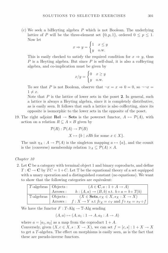
SOLUTIONS TO SELECTED EXERCISES 301
(c) We seek a biHeyting algebra P which is not Boolean. The underlyinglattice of P will be the three-element set {0, p, 1}, ordered 0 ≤ p ≤ 1.Now let
x ⇒ y =
{1 x ≤ y
y o.w.
This is easily checked to satisfy the required condition for x ⇒ y, thusP is a Heyting algebra. But since P is self-dual, it is also a coHeytingalgebra, and co-implication must be given by
x/y =
{0 x ≥ y
y o.w.
To see that P is not Boolean, observe that ¬x = x ⇒ 0 = 0, so ¬¬x =1 �= x.Note that P is the lattice of lower sets in the poset 2. In general, sucha lattice is always a Heyting algebra, since it is completely distributive,as is easily seen. It follows that such a lattice is also coHeyting, since itsopposite is isomorphic to the lower sets in the opposite of the poset.
19. The right adjoint Rel → Sets is the powerset functor, A �→ P(A), withaction on a relation R ⊆ A×B given by
P(R) : P(A) → P(B)
X �→ {b | xRb for some x ∈ X}.The unit ηA : A → P(A) is the singleton mapping a �→ {a}, and the counitis the (converse) membership relation &A ⊆ P(A)×A.
Chapter 10
2. Let C be a category with terminal object 1 and binary coproducts, and defineT : C → C by TC = 1+C. Let T be the equational theory of a set equippedwith a unary operation and a distinguished constant (no equations). We wantto show that the following categories are equivalent:
T -algebras Objects : (A ∈ C, a : 1 + A → A)Arrows : h : (A, a) → (B, b) s.t. h ◦ a = b ◦ T(h)
T-algebras Objects : (X ∈ Sets, cX ∈ X, sX : X → X)Arrows : f : X → Y s.t fcX = cY and f ◦ sX = sY ◦ f
We have the functor F : T -Alg → T-Alg sending
(A, a) �→ (A, a1 : 1 → A, a2 : A → A)
where a = [a1, a2] as a map from the coproduct 1 + A.Conversely, given (X, c ∈ X, s : X → X), we can set f = [c, s] : 1 + X → Xto get a T -algebra. The effect on morphisms is easily seen, as is the fact thatthese are pseudo-inverse functors.

302 SOLUTIONS TO SELECTED EXERCISES
Since free T-algebras exist in Sets and such existence is preserved by equi-valence functors, it follows that Sets has free T -algebras. In particular, aninitial T -algebra in Sets is the initial T-algebra N, which is an NNO.
3. Let i : TI → I be an initial T -algebra. By initiality, we can (uniquely) fill inthe dotted arrows of the following diagram:
TI .................Tu
� T 2IT i � TI
I
i
�...................
u� TI
T i
�
i� I
i
�
Composing the squares, we have a map of T -algebras I → I, which by uni-queness must be the identity. But then i ◦ u = 1I , and u ◦ i = Ti ◦ Tu =T (i ◦u) = 1TI , so i is an isomorphism. A natural numbers object N is initialfor the endofunctor TC = 1 + C, so it follows that N ∼= 1 + N for any NNO.

REFERENCES
The following works are referred to in the text. They are also recommended forfurther reading.
1. Eilenberg, S. and S. Mac Lane (1945) “General theory of natural equiva-lences,” Transactions of the American Mathematical Society 58, 231–94.
2. Johnstone, P.T. (1982) Stone Spaces, Cambridge: Cambridge UniversityPress.
3. Johnstone, P.T. (2002) Sketches of an Elephant: A Topos Theory Compen-dium, 2 vols, Oxford: Oxford University Press.
4. Lambek, J. and P. Scott (1986) Introduction to Higher-Order CategoricalLogic, Cambridge: Cambridge University Press.
5. Lawvere, F.W. (1969) “Adjointness in Foundations,” Dialectica, 23, 281–96.6. Mac Lane, S. (1971) Categories for the Working Mathematician, Springer:
Berlin, Heidelberg, New York, 2nd ed. 1998.7. Mac Lane, S. and I. Moerdijk (1992) Sheaves in Geometry and Logic: A First
Introduction to Topos Theory, Springer: Berlin, Heidelberg, New York.8. McLarty, C. (1995) Elementary Categories, Elementary Toposes, Oxford:
Oxford University Press.

This page intentionally left blank

INDEX
0, 81, 72, 7, 1513, 8, 88
adjoint, 209–250and orders, 221–223cocompletion as, 212examples of, 217–223existence of, 227, 241, 250exponential as, 217freeness as, 209image as, 222in a poset, 222left/right, 211limit as, 218open interior as, 221polynomial ring as, 220preservation of limits, 227product as, 211quantifiers as, 223rules of inference, 224
adjoint functor, 2Adjoint functor theorem, 241
special, 245adjunction, 2, see adjoint
counit of, 217Hom-set definition, 217preliminary definition, 210unit of, 211
AFT, see Adjoint functortheorem
algebra, 1, 4, 61and logic, 223boolean, see boolean algebrafor a monad, 261
and endofunctors, 274for an endofunctor, 268, 269
and monads, 274heyting, see heyting algebrainitial, 270, 273Lindenbaum-Tarski, 133presentation, 68, 69, 255
arrow, 4classifying, 201
associative law, 5
atomin a Boolean algebra, 179
automorphism, 12inner, 167
Beck’s theorem, 276bifunctor, 161biHeyting
algebra, 252BA, 151Boolean algebra, 34, 35, 51, 151, 153
finite, 179boolean algebra, 15, 129
Cantor, 273, 295Cat, 9, 24, 34, 147, 149
cartesian closed, 161category, 2, 4
algebraic, 266arrow, 16cartesian closed, 11, 122, 122–128, 168
and lambda calculus, 135equational, 134
cocomplete, 195comma, 243complete, 194, 244concrete, 7, 14, 150congruence, 84constructions on, 14–17coslice, 17, 26discrete, 11, 103, 149dual, 15Eilenberg-Moore, 261finite, 7finitely presented, 85–87free, 18–23, 27, 28homomorphism of, 8homomorphism theorem, 85Kleisli, 265, 279large, 24locally cartesian closed, 233, 237locally small, 25monoid, 11monoidal, 79, 168, 170
strict, 79
306 INDEX
category (cont.)of Boolean algebras, 151of categories, 9, 147of diagrams, 185, 202of elements, 196, 238of functors, see functor categoryof graphs, 166of groups, 80–83of indexed sets, 143of proofs, 10, 46of propositions, 252of subobjects, 90of types, 43, 136opposite, 15pointed sets, 17, 175poset, 9, 17preorder, 9product, 15quotient, 84skeletal, 183slice, 16, 177
and indexed families, 234small, 14, 24with limits, 104with products, 48, 46–48
category theory, 1–2, 8, 12, 23, 29, 38, 53,147
and adjoints, 209history of, 1
Cayley’s theorem, 13–14, 187CCC, see category, cartesian closedchange of base, 233choice
axiom of, 32, 51function, see function, choice
co-, 55coalgebra
for a comonad, 267cocompletion of a category, 229cocone, 105codomain, 4, 55coequalizer, 66, 65–71
of monoids, 70of categories, 148of monoids, 73of posets, 148of sets, 72of spaces, 73
cogenerating set, 245coherence theorem
for monoidal categories, 170coHeyting
algebra, 252boundary, 252negation, 252
cokernelof groups, 88
colimit, 105, 108–114creation of, 111
ω-colimit, 273colimits
of posets, 114comonad, 266, 266–267
and adjoints, 267component, 156composition, 4
of functions, 3computer science, 2, 10, 36concatination, 18cone, 101
as a natural transformation,166
congruence, 83–85, 88constant, 36C(X), 151contravariant, 107coproduct, 55, 55–61
of monoids, 59in a CCC, 193in a posets, 58injection, 55of categories, 147of groups, 60of monoids, 56of posets, 58of sets, 56, 109of spaces, 57
covariant, 48ωCPO, 112, 145
map of, 113strict, 145
Curry-Howard correspondence, 45,142
data type, 10deduction, 10, 131
transcendental, 164denotational semantics, 10, 138diagram
as a functor, 185commutative, 3hyperdoctrine, 253of a group, 77of type, 101product, 39pullback, 92
distributive law, 130and adjoints, 228
domain, 4, 55

INDEX 307
duality, 15, 53–55, 66, 71, 267and equivalence, 178conceptual, 54formal, 54in Sets, 160of vector spaces, 159principle, 53stone, 153–155, 178
Eckmann-Hilton argument, 78,88
elementgeneralized, 35–39, 91, 93global, 36variable, 36
endofunctor, 249, 257, 268–276epi, see epimorphismepimorphism, 29, 51, 67
of monoids, 31split, 32
equalizer, 62, 62–65of abelian groups, 65of functors, 147of monoids, 65of posets, 65of spaces, 65
equivalenceand duality, 178class, 65of categories, 172, 171–181
and isomorphism, 172relation, 65, 73, 90
equivalent categories, 172evaluation, 121exponent, 107exponential, 121, 119–140
in a poset, 129of categories, 161, 164of diagrams, 199of graphs, 125, 165of groups, 167of posets, 122of ωCPOs, 123
Fib, 240and presheaves, 240
fibration, 240field, 151filter, 35
maximal, 35ultra-, see ultrafilter
fixed point, 113, 271, 275forgetful functor, see functor, forgetful
foundations, 23–25free, 18
category, 20cocompletion, 198monoid, 18, 57, 209
monad, 264free algebra, 245Freyd, 241, 245Freyd, P., 253Fun, 158function, 1–3
bijective, 12characteristic, 63, 98, 152, 201choice, 33continuous, 6equality of, 4identity, 4injective, 5, 29monotone, 6recursive, 6, 248surjective, 29, 50
functor, 2, 8, 32, 147–149adjoint, see adjoint, see adjointcocontinuous, 229codiagonal, 148comonadic, 267comparison for a monad, 266composition of, 9constant, 166, 194continuous, 106contravariant, 107coproduct, 61embedding, 187endo-, see endofunctorexponential, 126factoring, 182faithful, 148forgetful, 16, 18, 21, 50, 148
adjoint, 246and limits, 111
full, 148identity, 9injective, 148monadic, 266morphism of, 155of groups, 83of posets, 10polynomial, see polynomial functor, see
polynomial functorprecomposition, 231product, 47product preserving, 49projection, 15representable, see representable functorset-valued, 185

308 INDEX
functor category, 158, 164–168, 185cocompleteness of, 195completeness of, 194of groups, 167of posets, 167
Galois connection, 221generator, 150generators, 21, 68
for a category, 85, 88for a CCC, 139insertion of, 18, 157
graph, 6, 27as a functor, 166, 186directed, 20of a function, 254underlying, 21
Graphs, 166graphs
category of, 125Grothendieck, 2group, 5, 6, 12, 15, 75–88, 149
abelian, 60, 72abstract, 75as a category, 83–85, 87factor, 81homomorphism theorem, 81in a category, 75–80, 87in lambda calculus, 80normal subgroup, 80ordered, 78permutation, 12representation, 83, 149structure, 150, 268topological, 78
Group, 25group theory, 1groupoid, 168groups
direct limit of, 109
heyting algebra, 129, 129–134and adjoints, 223
Hom-set, 11, 48, 48–50homomorphism
category, 8complete, 180graph, 21group, 13, 77, 149monoid, 12of algebras, 269ring, 35
ideal, 17adjoint, 233
identity arrow, 4image
direct, 222dual, 222inverse, 222
indexed family, 177and adjoints, 233–236
indexed sets, 143∫C P , 196, 238
interpretationof propositional calculus, 134
invariant, 37IPC, see propositional calculus, intuitionisticisomorphic, 12isomorphism, 12, 12–14, 20, 25, 26, 31
natural, 158
junk, 18, 20
Kan extension, 232Kan, Daniel, 209kernel
of a functor, 84of a group homomorphism, 82
Kleene closure, 18Kripke model, 240
of λ-calculus, 144Kripke semantics
for propositional calculus, 140
λ-calculus, see lambda calculuslambda calculus, 10, 43, 80, 135–140, 194,
240and CCC, 139completeness theorem, 138theory in, 137
Lambek’s lemma, 271, 277large category, see category, largelattice, 129Lawvere, 2, 223, 253Lawvere, F.W., 248LCCC, see category, locally cartesian closedlifts, 33limit, 102
creation of, 111direct, 109equalizer as, 103product as, 103pullback as, 104terminal object as, 103
lim−→, 109

INDEX 309
lim←−, 102limits, 100
and monomorphisms, 115by products and equalizers, 104of cardinality, 105of categories, 147of diagrams, 194preservation of, 105preserved by adjoints, 227
locally small category, see category, locallysmall
logic, 2, 10, 36, 46, 69, 80, 135, 194, 252algebraic, 223and adjoints, 223and topoi, 203categorical, 91first-order, 223higher-order, 194, 203intuitionistic, 131linear, 79, 170modal, 260, 267positive, 133
Mac Lane, 1, 38, 61Mac Lane’s pentagon, 170mapping, 6, 8
property, see universal mapping propertymodel
of propositional calculus, 134Mon, 11monad, 259, 255–279
algebra for, 261and adjoints, 255, 257, 261Eilenberg-Moore category, 261on a poset, 260powerset, 260
monadic, 266mono, see monomorphismmonoid, 11, 30, 59, 70, 271
and monad, 259free, 19, 18–20
monoidal category, see category, monoidalmonomorphism, 29, 51, 64, 89
as a limit, 115pullback of, 115split, 32
morphism, 5of T -algebras, 261of cocones, 109of cones, 102
Natural numbers object, 253natural numbers object, 248, 246–250, 271,
276
natural transformation, 2, 156, 157–161, 164naturality, 155–156Newton’s method, 113, 274NNO, see natural numbers objectnoise, 18, 20nonsense
abstract, 147numbers, 11, 12, 20, 247
ordinal, 171
object, 4generating, see generatorinitial, 33–35natural numbers, see natural numbers
objectprojective, 33, 51terminal, 33–36
objectsfamily of, 33
Ord, 171
Par, 175partial map, 175Π, 234point, 36, 175points
enough, 36polynomial functor, 269, 279
and trees, 272generalized, 270
Pos, 7, 25not monadic, 266
poset, 6, 30, 35, 57, 149complete, 130fibration of, 240
preorder, 9, 90, 245presheaf, 187product, 39, 38–48
cartesian, 39in a poset, 42of abelian groups, 60of categories, 42, 147of functors, 157of monoids, 42of posets, 42of sets, 41of topological spaces, 42
programming language, 10projective, see object, projectivepropositional calculus, 131–134, 194
and adjoints, 223completeness theorem, 134intuitionistic, 131

310 INDEX
propositional function, 98in a topos, 203
pseudo-inverse, 172pullback, 91, 91–100
and characteristic functions, 98and extensions, 98and reindexing, 99by products and equalizers, 94functor, 96, 178inverse image as, 94of sets, 94properties of, 95–100two, lemma, 95
pushout, 117of sets, 108
quantifiersgeometric interpretation, 225
quantifiers as adjoints, 203, 223–227quotient, 65, 66
of sets, 73
RAPL, 227–233recursion, 248, 271, 273reindexing, 234Rel, 7, 25relation, 7, 68
composition, 7identity, 7local membership, 91
relative product, 7representable functor, 48, 149, 187
and colimits, 107and limits, 106characterization of, 244contravariant, 107, 150
representation, 13, 187retract, 32retraction, 32, 32–33ring, 30
of functions, 151pointed, 220polynomial, 220
SAFT, see Adjoint functor theorem,special
Scott, Dana, 146section, 32, 32–33semigroup, 11set, 3, 11, 14
function, 120pointed, 17, 175
power, 34, 90, 130, 152, 260, 270as an adjoint, 251
structured, 6, 11, 30, 41, 188and functors, 186
set theory, 23Sets∗, 17, 175sets
cumulative hierarchy, 111family of, 99, 177, 233
Sets, 5, 24, 25cartesian closed, 122
SetsC, 185and adjoint functors, 231cartesian closed, 201cocomplete, 196complete, 194locally cartesian closed, 239slice category of, 238topos, 202
Setsfin, 5, 171, 179SetsI , 177SetsI , 233sieve, 202Σ, 234simplicial
nerve, 186, 204set, 186, 204
small category, see category, smallsolution set, 241space, see topological spaceStone duality, see duality, stoneStone duality theorem, 155Stone representation, 155Stone space, 181string, 265structure, 1, 29, 37, 151, 258
finitary, 269representable, 149–153
Sub, 90subcategory, 147
full, 148subobject, 89, 89–91
as an extension, 203classifier, 201, 205
for presheaves, 202
T -algebra, 245T -algebra, 255
for a monad, 261test object, 14, 36Top, 25topological space, 6, 42, 57, 130, 151, 267,
278Alexandroff, 182

INDEX 311
topological space (cont.)interior, 221
topologyspecialization order, 10, 26
topos, 202, 201–203, 254and logic, 203
transformationnatural, see natural transformation
transpose, 121tree, 271, 272triangle identities, 256, 255–257triple, see monadtwist, 158type theory, 43–45, 135–140, see lambda
calculusdependent, 240
ultrafilter, 35, 51, 107, 153, 179principal, 154
UMP, see universal mapping propertyunit law, 5universal, 19, 119
subobject, 201universal mapping property, 19, 21, 29, 39,
139and adjoints, 210of a congruence, 85of coequalizers, 66
of coproducts, 55of equalizers, 62of exponentials, 121of free categories, 23of free monoids, 19of function sets, 120of initial objects, 33of limits, 102of natural numbers, 248of polynomials, 221of products, 39, 51of pullbacks, 92of terminal objects, 33of Yoneda, 198, 229
vector space, 6, 30, 159finite dimensional, 160
well powered, 245word, 18, 60
empty, 18
Yoneda embedding, 187, 187–188, 192Yoneda lemma, 188, 193, 238Yoneda principle, 193