Overview of the temperature response in the mesosphereand lower thermosphere to solar activity

5

G. Beig 1 , J. Scheer2, M.G. Mlynczak3 and P. Keckhut4

1 Indian Institute of Tropical Meteorology, Pashan, Pune-411008, India (beig@tropmet.res.in )

2 Instituto de Astronomía y Física del Espacio, Buenos Aires, Ciudad Universitaria, Argentina

10 3 NASA Langley Research Center, Climate Science Branch, Hampton VA 23681,USA

4 Service d'Aeronomie - Institut Pierre Simon Laplace, University Versailles-Saint Quentin,

91371, Verrieres-Le-Buisson, Cedex, France

15 Abstract

The natural variability in the terrestrial mesosphere needs to be known to correctly quantify

global change. The response of the thermal structure to solar activity variations is an

important factor. Some of the earlier studies highly overestimated the mesospheric solar

20 response. Modeling of the mesospheric temperature response to solar activity has evolved in

recent years, and measurement techniques as well as the amount of data have improved.

Recent investigations revealed much smaller solar signatures and in some case no significant

solar signal at all. However, not much effort has been made to synthesize the results available

so far. This article presents an overview of the energy budget of the mesosphere and lower

25 thermosphere (MLT) and an up-to-date status of solar response in temperature structure based

on recently available observational data. An objective evaluation of the data sets is attempted

and important factors of uncertainty are discussed.

30

1

https://ntrs.nasa.gov/search.jsp?R=20090026490 2018-10-05T19:05:39+00:00Z

1. INTRODUCTION

The study of variation in atmospheric parameters due to several natural periodic and episodic

events has always been an interesting subject. It was realized recently that the perturbation of

35 atmospheric parameters caused by various human activities is not only confined to the lower

atmosphere but that it also most likely extends into the upper atmosphere [Roble and

Dickinson, 1989; Roble, 1995; Beig, 2000]. In view of this, it has become all the more

important and vital to study the variations due to natural activities in parameters affecting

climate to distinguish them from perturbations induced by global change.

40

Variations arising on decadal and even longer time scales may play a significant role in long-

term trend estimates. One of the major sources of decadal variability in the atmosphere is the

11-year solar activity cycle (as modeled by Brasseur and Solomon, 1986). Electromagnetic

radiation from the sun is not constant and varies mainly at shorter UV wavelengths on

45 different time scales [Donnelly, 1991]. Incoming solar radiation provides the external forcing

for the Earth-atmosphere system. While the total solar flux is quite constant, the UV spectral

irrandiance on the timescale of the 27-day and 11-year solar cycles exhibits the largest

changes, up to a factor of two over a solar cycle for the solar Lyman-a flux. Studies on the

changes in solar UV spectral irradiance on timescales of the 27-day and 11-year solar cycles

50 have been attempted by many workers in the past [Donnelly, 1991, Woods and Rottman,

1997, etc.]. It is believed that the essentially permanent changes arising in several

mesospheric parameters due to human activities are weaker whereas periodic changes due to

variations in solar activity are comparatively stronger [Beig, 2000].

55 The study related to the influence of solar activity on the vertical structure of temperature and

its separation from global change signals has been a challenge because only data sets of short

length (one or two decades) were available. The analysis of systematic changes in

temperature in the mesosphere and lower thermosphere has not been as comprehensive as in

the lower atmosphere. It is possible to suppress or even almost avoid the effects of solar cycle

60 on trend determination with the use of proper selection of the analyzed period combined with

the use of data corrected for solar and geomagnetic activity, or by comparison with empirical

models, which includes solar and geomagnetic activity, local time, season, latitude and

maybe some other parameters. The solar and geomagnetic activity may have a crucial impact

2

on the trend determination when data series are relatively short, or when we study trends in

65 the ionized component (ionosphere). Modeling of the mesospheric data series to extract the

solar cycle response has evolved with time, as improvements have been made in the

measurement techniques of the 11-year solar UV spectral changes. Most of the earlier

predictions overestimated the mesospheric response, since they were based on incorrect solar

UV-radiation derived from data of insufficient quality and/or length. This situation only

70 changed with the SME and UARS-missions, when the data became available to quantify the

variations since 1981. The modeling work of Chen et al. [ 1997] reported a solar cycle

response of several Kelvin in the mesopause region. The observed temperature variability at

70 km is not explicable in terms of corresponding 11-year changes in observed ozone

[Keating et al., 1987]. Searches for a strong dynamical feedback and attempts to invoke a

75 strong odd hydrogen photochemical heating effect, have so far not been successful. Until

recently, different data sets showed solar-cycle responses different even in polarity. The

limited availability of data sets and the comparatively short length of data records have been

the major constraints for mesospheric analysis. Nevertheless, during the past decade, a

number of studies have been carried out and more reliable solar signals in mesospheric

80 temperatures have been reported. It was thought earlier that it would be hard to identify a

trend in the MLT region if solar response is very large in magnitude, and that we needed

longer data sets encompassing several solar cycles. Recent investigations revealed the

presence of a solar component in MLT temperature in several data sets but probably they are

not as strong as expected. In recent times, a number of studies related to 11-year periodicities

85 in temperature of the MLT region have been reported [She and Krueger, 2004 and references

therein].

However, the solar response in temperature, if not properly filtered out, is still one of the

major sources of variation which may interfere with the detection of human-induced

90 temperature trends for the MLT region [Beig, 2002] and will have strong implication in the

quantification of global change signals. In recent time, the search for the effects of the 11-yr

solar cycle on middle atmosphere temperature has not led to consistent results that were easy

to interpret. Model studies suggest an in-phase response to the UV flux, peaking in the upper

mesosphere (2 K ampl.) and at the stratopause (1 to 2 K ampl.) [e.g., Brasseur, 1993; Matthes

95 et al., 2004]. However, the satellite analysis of Scaife et al. [2000] indicates a maximum

response at low latitude of about 0.7 K between 2 and 5 hPa (around 40 km), while that of

Hood [2004] shows a near zero response at 5 hPa but then increasing sharply to 2 K near 1

3

hPa. The increase of solar influence with altitude is not smooth. For example, the solar effect

in the mesopause region is relatively small (according to the model by Matthes et al., 2004;

100 but also according to several observations, see below), so it is easier to study long-term trends

in this region. It should be clear that if one does not account properly for the solar cycle

response, there can be biases for any remaining trend term. This concern is a particular

problem for any data time series that is not well-calibrated, not representative of seasonal or

global-scale processes, or not long enough.

105

Because of the very limited data not much effort has been made to synthesize the results

available in the past. Consequently, our knowledge of the quantification of solar response in

the temperature based on observations and model calculations for this region has been rather

poor. In view of this, it would be highly desirable that a consolidated status report for solar

110 trend in thermal structure for this region be prepared.

Before ground-based instrumentation with sensitive photoelectric registration and rocket-

borne in-situ measurements became available, the search for solar cycle effects with visual

airglow photometry in the 1920s, and with photographic spectrography, still dominant in the

115 1960s, is now mainly of historical interest. Reliable temperature determinations, by whatever

technique, became available only a few decades ago. Only recently, the detection of solar

activity effects in the upper atmosphere comes close to become a routine affair, and the

length of the available data sets is the main factor determining the quality of the results. In

order to arrive at a balanced overview of our present knowledge, it is therefore natural to

120 focus on the most recent results. These are also often based on the longest-duration data sets

of homogeneous quality. The reader interested in the historical development can find

references about early investigations of the atomic oxygen green line, which date back to the

1920s, and of subsequent Doppler temperature determinations since the mid-1950s, in

Hernandez [1976]. Other useful references focussing on green-line intensity variations can be

125 found in Deutsch and Hernandez [2003].

This article reviews the present status of observational and modelling evidence on the

response of the temperature structure in the region from 50 to 100 km to solar activity

variations. An objective evaluation of the available data sets is briefly attempted and

130 important uncertainly factors are outlined. We also discuss the lower thermosphere briefly.

For convenience, the whole region from 50-100 km is referred to as the MILT (Mesosphere

4

and Lower Thermosphere) region. The region from 50-80 km will be referred to as the

“mesosphere” and the region 80-100 km will be referred to as the “mesopause region”.

Understanding and interpreting the causes of atmospheric trends requires a fundamental

135 understanding of the energy budget. This is essentially the focus of the entire field of

tropospheric climate science, which is seeking to determine the extent to which human

activities are altering the planetary energy balance through the emission of greenhouse gases

and pollutants. We are just now at the point of being able to quantitatively assess the energy

budget in the MLT for the first time using the Thermosphere-Ionosphere-Mesosphere

140 Energetics and Dynamics (TIMED) mission and Sounding of the Atmosphere using

Broadband Emission Radiometry (SABER) instrument data.

2. OVERVIEW OF THE ENERGY BUDGET OF THE

MESOSPHERE AND LOWER THERMOSPHERE

145

Earth’s mesosphere and lower thermosphere are regions in which the transport and exchange

of energy occur through subtle and complex processes. The main inputs to the system are of

course provided by the Sun in the form of both photon and particulate energy. Ultraviolet

(UV) radiation from 1 to 300 nm is absorbed primarily by molecular oxygen and ozone in the

150 MLT. The variability of this portion of the spectrum with the 11-year solar cycle affects both

the thermal structure (through changes in the overall amount of energy deposited) and the

photochemistry of the MLT, especially the ozone abundance. Ozone is of particular

importance to the MLT energy budget. Through the absorption of solar radiation and as a

participant in exothermic chemical reactions ozone is responsible for up to 80% of the solar

155 and chemical heating of the mesosphere [Mlynczak, 1997]. Here we will provide a brief

overview of the energy budget of the MLT region in this section, following the corresponding

presentation in Beig et al. [2003] where more details are given.

The critical elements of the MLT energy budget are: heating due to the absorption of solar

160 radiation by O2, O3, and CO2; cooling due to infrared emission from NO, CO2, O3, H2O and

O; heating due to exothermic chemical reactions involving odd-oxygen and odd-hydrogen

species; energy loss due to airglow emission by O2( 1 Δ), O2( 1 Σ), CO2(4.3 gm) and OH(u). It is

important to distinguish the energy loss due to airglow from that which is characterized as

cooling. The energy in the airglow reduces the efficiency of solar or chemical reaction

5

165 heating – it never enters the thermal field, and hence is not acting to reduce the kinetic

temperature of the atmospheric gases. Finally, particle input, especially in the thermosphere,

is important, especially on short timescales and associated with solar flare or coronal mass

ejection (CME) events. A summary of key heating (solar and chemical) and infrared cooling

terms is given in Table 1.

170

The single most significant factor in differentiating the energy balance of the MLT from the

atmosphere below is that the density in the MLT is so low that collisions cannot always

maintain the processes of absorption and emission of radiation under local thermodynamic

equilibrium (LTE). Consequently, computation of rates of solar heating and infrared cooling

175 is a much more challenging process. In the case of solar energy, not all of the absorbed

energy is thermalized locally. This fact requires a detailed accounting of all possible

pathways for the absorbed solar energy to transit prior to ending up as heat or to being

radiated from the atmosphere as airglow without ever having entered the thermal field. Thus

we say that the efficiency of solar heating is substantially less than unity due to these

180 processes, to as low as 65%. The details of the solar and chemical heating and the associated

efficiencies are reviewed by Mlynczak and Solomon [1993].

In the case of radiative cooling, the effective temperature at which infrared active species

radiate is not given by the local kinetic temperature. This fact requires extremely detailed

185 consideration of the exchange of energy (thermal, radiative, chemical) between the infrared

active molecules and their environment for a multitude of quantum energy states within each

molecule [e.g., López -Puertas and Taylor, 2002]. The key radiative cooling mechanisms in

the MLT involve several infrared active species including the molecules CO2 and O3 [Curtis

and Goody, 1956], H2O [e.g., Mlynczak et al., 1999], NO [Kockarts, 1980], and atomic

190 oxygen (O) [Bates, 1951]. Of these, the CO2, O3 , and NO emissions exhibit substantial

departure from LTE in the MLT. The water vapor and atomic oxygen emissions correspond

to transitions in the far-infrared portion of the spectrum (wavelengths typically longer than 20

gm) that are more readily thermalized by collisions, and thus maintained in LTE.

195 The solar photon energy is the dominant source of energy into the MLT, but the solar

particulate energy is nevertheless important. While the photon energy from the Sun varies on

relatively long timescales (from the 27-day solar rotation to the 11-year sunspot cycle),

6

particulate energy from the Sun varies in a much more erratic (and often violent) way. Recent

observations of the thermospheric and mesospheric response to variations in particle input

200 from CME events clearly indicate the potential to alter the thermal structure and the radiative

cooling mechanisms. Seppälä et al., [2004] and Rohen et al., [2005] have observed the

destruction of ozone in response to strong solar storm events. In the stratosphere and lower

mesosphere, radiative cooling by ozone is critical to the energy balance. Thus there is a direct

impact on the energy balance in the stratosphere from solar particle precipitation.

205

From this overview of the energy budget, it is clear that the variability of solar radiation input

into the MLT region may impact the thermal structure directly (through the increase or

decrease in the total amount of solar energy deposited) and indirectly, for example, by

modifying the ozone abundance and thereby the heating and cooling rates. It is specifically

210 because of the complexity of the energy budget that assessing and attributing observed

changes (cyclical and secular) in the MLT is a formidable scientific challenge.

3. TECHNIQUES AND OBJECTIVE EVALUATION OF

TEMPERATURE DATA SETS

215

In addition to the satellite datasets, there are a number of experimental data records from

ground based or in-situ observations of mesospheric temperatures, although the mesospheric

record is still small compared to what is available at lower altitudes. The same techniques and

associated measuring uncertainties that are discussed by Beig et al. [2003] for their use in

220 trend analyses are also relevant, to some extent, in the present context, so we can make

reference to the greater detail given there.

In addition to ground-based observations which are capable to supply long data sets at fixed

geographic locations, also in-situ data from rocketsondes and global observations from

225 satellites can be used to measure temperature suitable for the detection of solar activity

effects. Details of all the data sets obtained during the past few decades and available for

evaluation of temperature trend in the MLT region are also given in Beig et al. [2003]. Figure

1 shows most of the known ground based locations of long term temperature measurements

all over the globe. The techniques applied to measure the temperature are also indicated as far

230 as possible. As mentioned in Beig et al. [2003], even for standard instrumentation used for a

7

long time, technical improvements can introduce uncertainties when data obtained at different

times are combined into longer data sets. While this can be most serious for long-term trend

detection, it can also interfere to some extent with the determination of solar activity

response. Techniques capable of supplying data over an extended height range like rocket-

235 launched or lidar temperature or density soundings (from which temperature profiles can be

derived) nevertheless suffer from an inevitable loss of precision at the greatest altitudes,

where they often cannot compete with ground-based observations. The long time span

covered by some ground-based measurements makes them particularly useful to study solar

cycle variations.

240

Mesopause region temperature is most often determined from line intensity measurements in

hydroxyl (OH) airglow bands of the airglow, but the so-called Atmospheric band of

molecular oxygen is now quite often also used. These rotational temperatures agree with

kinetic temperature at the peak of the vertical airglow emission profile. According to

245 measurements with many different techniques, the OH emission comes from an emission

layer at 87 km with a mean thickness of 8 km [Baker and Stair, 1988; more references are

given in Beig et al., 2003]. Satellite limb scans have resulted in reports on height variations

by several kilometers which may be related to dynamics [e.g., Liu and Shepherd, 2006], and

Nikoukar et al. [2007] have found recently that the bands from the upper vibrational levels 7,

250 8, and 9 come from an altitude slightly higher than the bands from the 4, 5, and 6 levels.

According to these results, the difference is 1.9 ± 1.4 km, while the mean peak altitude for the

latter bands (which are probably representative of the most widely used ground-based

observations) is consistent with the nominal values mentioned above. The observed

variability does not invalidate ground-based measurements of hydroxyl rotational

255 temperature as a useful tool to diagnose atmospheric temperature trends or solar activity

effects, as long as this variability can be treated as random, or be considered as part of the

phenomenon. The same holds for the O 2 Atmospheric band, with a nominal emission peak

height of 95 km.

260 From OH or O 2 airglow observations, temperature precisions of a few Kelvin can be obtained

with integration times not longer than a few minutes. Therefore, by averaging over a number

of individual measurements, the contribution of instrumental noise to the mean temperature

can easily be made negligible. Systematic errors affecting data accuracy have only an

influence on trend or solar activity results if they vary with time. They are not a problem if

8

265 long-term stability can be assured, and one way to ensure stability is with good instrument

calibration. The discussion about this point in Beig et al. [2003] is mostly important in the

context of the possibility to detect small long-term trends. For detecting effects of the 11-year

solar cycle, which has a rise time of only about four years, and where responses of several

Kelvin have been reported, the instrument stability requirements are less stringent. The

270 relative calibration of the instrument response at two or more wavelengths necessary for

determining rotational temperature is not difficult.

The rotational temperatures in the mesopause region vary on time scales from a few minutes

for short-period gravity waves to the solar cycle, and beyond. Nocturnal mean temperatures

275 used as the basis for solar cycle and trend analysis are affected by the short-term variability

only as far as gravity waves and variations due to the thermal tide are not completely

cancelled out. This “geophysical noise” can be expected to be quite variable and so create

only small uncertainties on longer time scales. There is however also a day-to-day variability

from planetary waves and unknown sources which could not be avoided even if

280 measurements over complete nights were always available. This underlines the importance of

dealing with airglow temperature data sets based on the greatest possible number of nights.

The same obviously also holds for data sets from other techniques.

Apart from O2 rotational temperatures, some data sets extend the information available above

285 the altitude of OH by using atomic line intensities from sodium or atomic oxygen as a proxy

for temperature, based on an empirical correlation between intensity and temperature (see,

e.g., Golitsyn et al., [2006]). The validity of this approach is questionable and cannot be

recommended as a replacement for direct temperature measurements, be it by the

measurement of O2 rotational temperature, of Doppler width with Fabry-Perot instruments, or

290 by laser spectroscopy with sodium lidars.

The length of the data set required for determining solar signatures may be as short as the few

years that the solar cycle takes to ascend from minimum to maximum, but may also be as

long as several cycles, if the effect is small compared to other variability (for example,

295 seasonal) , or is itself strongly variable. The data sets from different measurement techniques

vary widely not only in the number of years covered, but even more so with respect to the

uniformity of coverage and the number of individual data points available. Some airglow data

sets consist of millions of individual, statistically independent observations at a fixed site,

9

resulting in up to about 5000 nocturnal means, all referring to the same (nominal) altitude. On

300 the other hand, rocket soundings yield only one profile per launch, and from less than 100 to

several hundred profiles may be available from a given site, but a considerable altitude range

is covered. As pointed out before, lidar soundings (either by Rayleigh lidars covering a wide

range of altitudes similar to rocketsondes, or by sodium lidars that are limited to the

mesopause region) can easily surpass the number of profiles from rockets, being limited only

305 by clear weather requirements, and not by equipment expense. Finally, satellite observations

easily comprise millions of vertical temperature profiles, with near-global coverage, but the

number of overpasses at a given site is very much lower, refers to only slowly varying local

time, and the available long-term coverage is still small. The SCIAMACHY instrument on

Envisat is capable of measuring OH rotational temperature by limb sounding [ von Savigny et

310 al., 2004]. It was launched only in 2004, but can be expected to contribute data on solar

activity response in the near future.

4. OBSERVATIONS OF THE SOLAR RESPONSE IN THE

315 MESOSPHERE

The response of temperature and the middle atmosphere species to 11-year solar UV

variations has been difficult to isolate using satellite data. This is partially due to the short

time series of satellite data sets relative to 11-year variations, to instrument drifts, and to the

320 strong longitudinal variability that makes zonal means appear quite noisy [see Chanin, 2006].

On this time scale the quasi coincidence of the recent major volcanic eruptions with solar

maximum [Kerzenmacher et al., 2006] conditions increases the challenge while indirect

mesospheric responses were observed [Keckhut et a.l, 1995, 1996]. This effect was caused by

changes to the wave propagation induced by the thermal forcing inside the volcanic cloud and

325 vertical stability around the tropopause [Rind et al., 1992]. In the past, only rocket

temperatures have provided such long data sets in the mesosphere. However, the required

aerothermic corrections and changes of the sampling and time of measurements induce some

bias mainly in the mesosphere. More recently Rayleigh lidars that are much less expensive

and require less resources for continuous operations have replaced the rocket techniques.

330 From space, HALOE aboard UARS is the only experiment that allows mesospheric

temperature over more than a decade with a single instrument. However, while global, the

10

number of solar occultation does not provide such a large sampling as desirable.

The solar activity is also modulated by the solar rotation, and UV series exhibit strong

335 responses with periods of 27 days and harmonics. On this scale more temperature series are

available. From the ground, rockets and lidars can be used. However, lidars are more

adequate to perform daily series while typical rocket sampling is close to a week. The

experiments on board Nimbus 6 and 7 were used intensively to retrieve stratospheric and

mesospheric temperature responses. However, these changes related to the solar rotation

340 present smaller amplitudes than the solar cycle and are highly non-stationary. In the case of

the sun, the physical processes governing the evolution of active regions and the resulted

variations in the solar output are, at best, only quasi-stationary over a limited time period.

On the time range of solar cycle the radio flux at 10.7 cm is used as proxy of solar activity

345 while long–term UV measuremeots from space are not available. On the other hand, the

short-term solar UV variation is not well described by standard radio solar flux at 10.7 cm

and more direct UV measurements from space at 205 nm, Lyman alpha or proxies such as

Magnesium Lines Mg II are preferred to better describe daily changes of solar UV (see

Dudok de Wit et al., [2007] for a recent investigation of this topic). While in the middle

350 atmosphere, ozone and temperature are highly connected due to thermal ozone absorption

and thermal sensitivity of the ozone dissociation, the simultaneous investigations of ozone

and temperature allow for a better understanding of the middle-atmosphere response to solar

activity changes. Ozone measurements on Solar Mesosphere Explorer (SME) and on Nimbus

7 were analyzed. At high latitudes, direct ozone response (and hence temperature) to solar

355 activity variations may also be overwhelmed by solar proton events. The satellite sensors for

solar EUV may also occasionally be saturated by solar particles [e.g. see an example in

Scheer and Reisin, 2007].

In photochemical models, the ozone sensitivity on the 27-day and the 11-year scale are

360 similar because the time constant of ozone is negligibly short, in comparison. However,

discrepancies exist when including temperature-chemistry feedback in the model

calculations. It is possible that this is indicative of an indirect dynamical component of the

solar response.

11

365 4.1 Changes due to 27-Day UV Solar Forcing

Temperature variations are affected by a number of short-term dynamical influences

independent of solar variations, and thus it is more difficult to isolate the solar signal.

Temperatures are available simultaneously from the SAMS instrument on the Solar

370 Mesosphere Explorer (SME) satellite. In the ±20' latitude band at 2 mbar a temperature

variation of 1.5K for 10% ozone change is reported, which grows to 2.5K at 70 km. In

contrast to the stratospheric maximum that is limited to the ±20' latitude band, this second

maximum in the mesosphere is present in the ±40' latitude band. The observed temperature

phase lag with 205 nm solar flux is shorter than 1 day in the mesosphere, and the altitude of

375 maximum temperature sensitivity is close to the altitudes of maximum ozone depletion.

Therefore, in addition to the HO x effect on ozone, the temperature sensitivity can be expected

to play a role through temperature feedback or as a consequence of the solar Lyman alpha

heating. This mesospheric maximum was not predicted by numerical models but must be

real, since Summers et al. [1990] conclude that the discrepancies between model and

380 observation cannot be explained by data-related errors. At mid-latitudes, wavelet analysis of

lidar time series [Keckhut and Chanin, 1992] shows that planetary waves tend to mask the

direct solar response in temperatures since wave amplitudes are large and periods may be

comparable to the solar rotation period; planetary waves exhibit periods from a few days to

30 days. On the other hand, planetary waves may be directly involved in the solar forcing

385 (see below).

Ebel et al. [ 1986] have suggested that the generation of vertical wind oscillations in the 27-

day period range would at least lead to the right sign of correlation (through adiabatic cooling

during the upward wind phase and simultaneous transport in the direction of the vertical

390 ozone mixing ratio gradient in the lower dynamical regime and photochemical increase at

higher layers due to the temperature dependence of the ozone reaction coefficients). This

effect may also be responsible for the fact that the ozone perturbations inferred from UV flux

changes are better reproduced by simulations without temperature feedback than with it

[Keating et al., 1987] due to the compensating effect of adiabatic heating.

395

Radiance measurements were made with the Pressure Modulated Radiometer (PMR) on

board NIMBUS 6 [Crane, 1979]. Maximum values obtained for the 27 day periodicity were

12

1.5 K near the mesopause, 3.0 K in the lower mesosphere and 3.5 K in the upper stratosphere,

at latitudes between about 50° and 70° [Ebel et al., 1986]. Since indirect perturbations seem

400 to exceed the direct ones in amplitude, non-linear interactions of forced variations with the

atmospheric system also have to be considered. Furthermore the large spatial scales of the

possible solar activity effects showing up in the global and hemispheric data sets employed in

this study support the view that planetary waves are an essential part of the unknown

mechanisms.

405

4.2 Changes on the 11-Years Solar Scale

The atmospheric temperature response to solar UV changes is expected through ozone and

oxygen absorption processes in the middle atmosphere. In the stratosphere, the response

410 shows a positive correlation between the temperature and the solar activity with an effect of

1-2 Kelvin in the upper stratosphere due to ozone photolysis and solar absorption, while at

higher latitude negative responses are reported [Keckhut et al., 2005]. These observations

confirmed by rocket series could be explained by dynamic feedbacks and more specifically

by the occurrence of stratospheric warmings [ Hampson et al., 2005]. From this numerical

415 simulation, a positive effect is expected in the mesosphere. Because the winter response

results in a dynamic feedback, the signature is expected to be non-zonal in the northern

hemisphere [Hampson et al., 2006]. While stratospheric warmings are associated with

mesospheric cooling, it is not surprising to see these alternating patterns at mid and high

latitudes [Matsuno, 1971]. In the tropical mesosphere, a response can be also expected, as

420 tropical mesospheric anomalies associated with stratospheric warmings are also reported

[Sivakumar et al., 2004, Shepherd et al., 2007]. A summary of the solar response in the

mesosphere is given in Table 2.

The search for a solar trend in the mesosphere had started in the late 70s when a few authors

425 reported solar cycle associated variability in mesosphere temperatures. Shefov [1969]

reported a solar cycle variation in OH rotational temperature on the order of 20-25 K for mid-

latitudes. Labitzke and Chanin [1988] using rocketsonde data at Heiss island located at 81°N

reported solar cycle temperature variations on the order of 25K at 80 km. Kubicki et al.

[2007] have reanalyzed the same set of data and deduced a negative solar response of several

430 kelvins. The time series of Russian rocketsonde measurements at four different sites

13

(covering low to high latitudes) revealed a substantial positive solar response in the

mesosphere [Mohanakumar, 1985, 1995]. However, in recent time, results are found to be

quite different. The reanalysis of the Thumba (8°N) tropical data extending to more than two

solar cycles [Beig and Fadnavis, 2003] has recently also resulted in a positive solar response

435 of temperature in the mesosphere but of much lower magnitude than reported earlier [ Kokin

et al., 1990]. US rockets have shown a clear solar response in the upper stratosphere

[Dunkerton et al., 1998]. In the mesosphere only 2 subtropical sites allow to retrieve the solar

response in the mesosphere. A positive correlation has been found with a temperature

response of 2 K on a large latitude range from 50 to 70 km [Keckhut et al., 1999].. An

440 analysis of falling sphere and rocket grenade data by Lübken [2000, 2001] revealed no

statistically significant solar component for the altitude range 50-85 km, however the analysis

only included data during the summer season. Remsberg and Deaver [2005] have analyzed

long-term changes in temperature versus pressure given by the long time series of zonal

average temperature from the Halogen Occultation Experiment HALOE on the Upper

445 Atmosphere Research Satellite (UARS). The HALOE temperature data are being obtained

using atmospheric transmission measurement from its CO2 channel centered at 2.8

micrometers [Russell et al., 1993, Remsberg et al., 2002]. While the length of the data set is

still short, they have reported a mesospheric response of 2-3 K around 70-75 km. In a more

recent work Remsberg [2007] found more accurate results ranging from 0.7 to 1.6 K in the

450 lower mesosphere and from 1.7 to 3.5 K in the upper mesosphere. In mid-latitude responses

are larger and in the tropical latitude band only 0.4 to 1.1 K is reported. The long-term series

of lidar data obtained at Haute Provence (44°N) has revealed a positive (in phase) solar

response of 2 K/100 sfu (solar flux units) in the mesosphere up to 70 km. The response was

found to fall off with height above 65 km, with a tendency towards a negative response above

455 80 km [Keckhut et al., 1995].

Atmospheric temperature response to the 27-days and 11-years solar cycle as function of

altitude from different studies focus on tropical regions are shown in Figure 2. SAMS

[Keating et al., 1987] and PMR [Ebel et al., 1986] analyses are performed on the solar

460 rotation time scale. HALOE analyses above the ±20° latitude band [ Remsberg, 2007] concern

the 11-years time scale. Two different analyses [ Beig and Fadvanis, 2003; Kokin et al., 1990]

have been used to analyze the data of the rocket station Thumba (8.5 oN, 77oE)..

14

Atmospheric temperature response to the 11-years solar cycle as a function of altitude from

465 different studies covering mid-latitudes are shown in Figure 3. Error bars associated with the

OHP lidar correspond to the range of seasonal changes [ Keckhut et al., 2005]. The hatched

area corresponds to the HALOE observations in different latitude bands [Remsberg, 2007].

The US Rocket corresponds to an average of 3 subtropical rocket stations [Keckhut et al.,

1999]. The Soviet rocket sites (Heiss, Volgograd and Molodezhnaya) data have been

470 analyzed by Kokin et al. [1990] and Golitsyn et al. (2006). They obtained different solar

response for different stations as shown in Figure 3.

4.3 Seasonal Variations

475 Mohanakumar [1995] shows the summer response varied in the same way with latitude

between Arctic and Antarctic but was about half the wintertime values. The Thumba results

indicate also a stronger positive solar component in winter as compared to summer for the

mesosphere, which is in agreement with mid-latitude lidar results [ Keckhut et al., 1995].

Hauchecorne et al. [1991] had already reported earlier that solar response changes sign from

480 winter to summer depending on height, using lidar data (1978-1989) at heights from 33 up to

75 km. They found about 5 K/100sfu during winter for 60-70 km altitude (where the

maximum response is observed) and for summer about 3K/100sfu. Later, Keckhut et al.

[1995] using data from the same lidar for an extended period reported the solar response over

a height range of 30-80 km for summer, with a negative tendency at height above 75 km. In

485 the mesopause region, the changes of the response to solar activity during the specified

intervals occur most distinctly in autumn, winter and spring. For summer, the response of the

atmosphere does not practically change, though it has the maximal value. Therefore the

dispersion of the values mentioned above is probably caused by the seasonal nature of

observation. Golitsyn et al. [2006] have recently analyzed the response of the monthly mean

490 temperature data on the solar activity variations for the altitudes 30-100 km. They obtained

the minimal solar response at heights ~55-70 km with a value of +2±0.4 K/100sfu for winter

and -1±0.4K/100 sfu for summer.

495

15

4.4 Atmospheric Response due to Solar Flares

During major solar flare events, energetic particles penetrate down into the Earth’s

mesosphere and upper stratosphere. By ionizing molecules, solar proton events (SPE) are

500 expected to produce a large enhancement of odd nitrogen at high latitudes in the mesosphere

[Crutzen, 1975; Callis et al., 2002]. Odd nitrogen species play an important role in the

stratospheric ozone balance through catalytic ozone destruction. In the upper stratosphere and

mesosphere, ozone decreases of 20 to 40% associated with SPE have been reported [ Weeks et

al., 1972; Heath et al.,1977; McPeters et al., 1981; Thomas et al., 1983, McPeters and

505 Jackman, 1985]. When a strong stable polar vortex forms, diabatic descent inside the vortex

can transport NOx rapidly downward, and may enhance the effect of ozone destruction

[Hauchecorne et al., 2005]. As expected from numerical models [Reagan et al., 1981; Reid

and Solomon, 1991] simultaneous cooling of around 10 K in the lower mesosphere was

observed by Zadorozhny et al. [1994], in October 1989, using meteorological M-100B

510 rockets, while NCEP temperature analyses [Jackman and Mc Peters, 1985] report no

detectable temperature decrease associated with the event of July 1982.

A recent search for a response of the mesopause region to solar flares and geomagnetic

storms by Scheer and Reisin [2007] in the airglow data base from El Leoncito (32 oS, 69oW)

515 revealed no convincing evidence, in spite of the coverage of very strong solar and

geomagnetic events. There is however the possibility that the atmospheric response (at the

relatively low latitude) is only short-lived and therefore limits detection by nocturnal

observations to cases of favorable flare timing. If this is so, daytime observation techniques

would be more suitable for detecting flare effects in the mesopause region.

5. OBSERVATIONS OF THE SOLAR CYCLE RESPONSE IN THE

MESOPAUSE REGION

5.1 Annual mean response

The majority of the results discussed in this section are obtained from measurements of OH

airglow which correspond to nominal altitudes of 87 km. Section 4 of the Beig et al. [2003]

520

525

16

paper contains information on some earlier solar activity studies since the 1970s, with an

emphasis on OH rotational temperature, only part of which will therefore again be discussed

530 here.

Sahai et al. [1996] reported a solar activity effect of 32 K/100sfu from OH airglow

temperature measurements at Calgary (51 oN, 114oW) based on the comparison of two low

activity years (1987, 1988) with a high activity year (1990). The solar signal found by

535 Gavrilyeva and Ammosov [2002] from their OH data obtained at Maimaga (63 oN, 130oE)

between 1997 and early 2000 was only one third as great as the result from Calgary, but is

still a high-end result (11 ±3 K/100sfu), when compared to the other solar temperature

responses observed all over the globe, that were published in recent years. Both results may

be considered problematic because of the short time span covered, in combination with the

540 strong seasonal variability, characteristic of medium and high latitudes. They are not

automatically discredited by disagreeing with the lower values found elsewhere, because they

could only be refuted by observations under the same conditions. Similar arguments can be

used in favor of the strongly negative solar cycle effects in O I Doppler temperatures (ca. –30

K/100sfu) by Hernandez [1976] at mid- and low latitudes, and by Nikolashkin et al. [2001],

545 at Maimaga (ca. –15 K/100sfu), although those latter authors’ result for OH temperature (+5

K/100sfu for eastward QBO phase, -30 K/100sfu for westward) is somewhat at odds with the

more recent data by Gavrilyeva and Ammosov [2002] from the same site.

Figure 4 and 5 show the solar response in temperature (K/100sfu) as reported by different

550 authors using various experimental data in recent time for the Northern and Southern

Hemispheres, respectively. For easier reference, the pertinent details corresponding to each

result are also listed in Table 3.

Sigernes et al. [2003] found no solar signal in the time series of OH airglow data from the

555 auroral station Adventsdalen (78 °N, 1 5 ° E) that span 22 years. On the other hand, in the mid-

latitude Northern Hemisphere, where the greatest number of OH airglow temperature

measurements is available, all studies signal a positive response to solar activity. Espy and

Stegman [2002] have initially not reported an appreciable solar cycle effect at the height of

the OH layer over Stockholm (59 °N, 18°E), but after a new analysis that includes more recent

560 data, these authors find evidence for a positive effect of about 2 K/100sfu (1.6 ± 0.8

17

K/100sfu, in winter); [P.J. Espy, 2007, personal communication]. New results from

Zvenigorod (56°N, 37°E), for the years 2000 – 2006 reported by Pertsev and Perminov

[2007] indicate an annual mean response of 4.5 ± 0.5 K/100sfu, which is somewhat stronger

than previous results partly derived from the same site [ Golitsyn et al., 2006, see below].

565 The recent analysis by Offermann et al. [2004] based on 21 years of OH airglow temperature

data for Wuppertal (5 1 °N, 7° E) extends up to 2002 and now covers almost two solar cycles.

This long series of observations was started in 1980 with the aim to determine solar and long-

term trends in the mesospause region. The authors found an effect of 3.0 ± 1.6 K/100sfu, on a

monthly basis, from temperature enhancements during the maxima of two solar cycles. The

570 authors assumed a linear correlation between temperature and solar activity, ignoring

possible lags. The annual mean response is 3.4 K/100sfu.

Bittner et al. [2000] analyzed the Wuppertal (51 °N, 7°E) data for the period 1981-1995 with

respect to temperature variability with periods of several days, but not with respect to

575 absolute temperature (as most other studies). They found positive solar correlation response

for temperature oscillations with periods greater than ~30 days and negative correlation for

periods less than ~10 days. In an analysis of the complete Wuppertal data set including the

year 2005 [Höppner and Bittner, 2007] , the 11-year solar signal for the period range from 3

to 20 days had disappeared, but there was, surprisingly, evidence for a correlation with the

580 22-year heliomagnetic cycle. The authors investigated the possibility of a magnetic coupling

between the solar and terrestrial magnetic fields, and indeed found a weak modulation in the

Earth’s rotation period with a shape similar to the observed variation of the standard

deviation of OH temperature. Lowe [2002] has made OH layer measurements for one full

solar cycle at Delaware Observatory (43 °N, 81 °W) in Canada and found a positive solar

585 response of 1.5 ± 1.1 K/100sfu.

Golitsyn et al. [2006] have consolidated Russian results from their earlier analysis [ Golitsyn

et al., 1996] based on the rocket data from Volgograd (49 oN) and data from different airglow

emissions obtained at Abastumani (42 ºN) and Zvenigorod (56 ºN), covering two activity

590 cycles (1976-1991). Monthly and annual mean model profiles of the temperature response to

the solar cycle where fitted to these data, which at the altitude of 87 km are based essentially

on OH rotational temperatures. The annual mean response is about 2.7 ± 1.7 K/100sfu, with a

tendency to grow with altitude.

18

595 An alternating negative and positive temperature response is consistently found in Northern

Hemisphere mid-latitude results obtained by incoherent scatter radar, Rayleigh lidar [ Chanin

et al., 1989], and sodium lidar [She and Krueger, 2004] for altitudes between 30 and (in some

data sets as high as) 140 km. This suggests that dynamical coupling from the troposphere to

the thermosphere is involved in solar activity induced signatures. She and Krueger [2004]

600 have recently reported the impact of 11 year solar variabilities on the mesopause region

temperature over Fort Collins (41 oN, 105oW) using their sodium lidar data obtained between

1990 and 2001. They found no solar signal at 83 km, but a positive effect of 3 ± 2 K/100sfu

at 87 km (updated numbers according to C.-Y. She, personal communication [2007]). The

HALOE results by Remsberg and Deaver [2005] mentioned above also refer to the lower

605 limit of the mesopause region. For different latitude zones, 11-yr solar cycle terms with

amplitudes of 0.5 to 1.7 K were found for the middle to upper mesosphere (80 km).

Figure 5 shows the solar response in temperature for the Southern Hemisphere. Clemesha et

al. [2005] reported the OH rotational temperature measurements made at Cachoeira Paulista

610 (23oS, 45 oW) for the period from 1987 to 2000. A simultaneous linear and 11-year sinusoidal

fit resulted in a solar cycle amplitude of 6.0 ± 1.3 K with maxima in 1990 (and therefore also

in 2001), well in phase with solar activity. The linear trend of 10.8 ± 1.5 K / decade agrees

perfectly well with the results obtained for nearly the same time span and geographic area (El

Leoncito, 32oS, 69 oW) by Reisin and Scheer [2002]. Clemesha et al. [2005] also found a

615 positive OH intensity trend of the order of 1.9%/year, which, in view of the combined error

bounds, is not considerably above the intensity trend observed by Reisin and Scheer (about

+1%/year). However, the strong solar cycle signature found by Clemesha et al. [2005]

(expressed as 11-year amplitude) that can be estimated to correspond to about 8-10 K/100sfu

is at odds with the near-zero effect enountered by Reisin and Scheer [2002]. The Leoncito

620 results are confirmed by the most recent analysis of OH (6-2) rotational temperatures and

airglow brightness variations during the rise and maximum phase of solar cycle 23 [ Scheer et

al., 2005]. No solar cycle signature was found, but when a temporal trend is allowed for, the

solar effect may approach 1.4K. The disagreement with the solar response at Cachoeira

Paulista may be a consequence of latitudinal differences in planetary wave activity, and

625 therefore need not be considered contradictory.

19

Results about OH temperatures from Davis (69°S, 78°E) will be discussed in the next section.

Hernandez [2003] measured the polar mesospheric temperature above South Pole (90oS)

from 1991-2002 using the Doppler width of the OH line at 840 nm by means of a high-

630 reolution Fabry-Perot interferometer and deduced a solar signal as high as 13K/100sfu. This

is the strongest solar temperature signal reported in recent years. From the same site, Azeem

et al. [2007] have reported OH rotational temperatures obtained during the austral winters of

1994–2004. In spite of the temporal overlap between both data sets, the comparable coverage

of data, and the expected approximate equivalence of the temperatures obtained by both

635 techniques, the solar cycle effect of 4.0 ±1.0 K/sfu reported by Azeem et al. [2007] is only

about one third of the result obtained by Hernandez [2003]. The reason for this discrepancy is

unknown. Figure 6 provides the summary of the solar response in temperature for the lower

thermosphere. In this height range, the results obtained by Golitsyn et al. [2006] depend in

part on temperatures estimated from the brightness of different airglow emissions, and in part

640 on the extrapolation of OH temperature response to greater heights. Their composite profile

indicates an annual mean solar response of 2.8K/100sfu and 2.3K /100 sfu for the altitudes

of 92 km and 97 km respectively. She and Krueger [2004] have found a solar signal of

4K/100sfu between about 92 and 98 km. Above 101 km, the effect decreases quickly to zero

at 103 km and becomes negative at 104 km. The mean solar cycle effect in O 2 rotational

645 temperatures measured at El Leoncito (32 oS, 69oV) [Scheer et al., 2005] is consistent with

the range of upper limits estimated earlier [ Reisin and Scheer, 2002]. A positive response of

3.3 ± 0.3 K/100sfu is reported (which would reduce to 1.32 ± 0.3 K/100sfu, if a temporal

trend is simultaneously fitted). The authors conclude however that the mean values are

however only the net effect of successive short-term spells of anti-correlation, the absence of

650 correlation, each lasting many months, and a 32-months regime of strong correlation. So,

there is obviously no seasonal regularity in the solar signal at this site. All these recent results

for northern and southern mid-latitudes that refer to heights around 95 km compare quite well

with each other, although they are obtained by quite different techniques.

655 5.2 Seasonal Differences

As mentioned above, the results reported by Golitsyn et al. [2006] are seasonally resolved,

and solar response changes with season (even in sign) and assumes the most extreme values

(both positive, and negative) in the mesopause region, at heights of about 80-95 km.

20

660 Response is most variable in autumn, winter and spring, and a strong, but stable response

prevails in summer. These authors deduced a solar response of -5 ± 1.7 K/100sfu for winter,

and 8 ± 1.7 K/100sfu for summer, in this altitude range.

The absence of a solar response in the OH data from Adventsdalen (78 °N) for winter was

665 already mentioned [Sigernes et al., 2003, and also Nielsen et al., 2002]. Lübken [2000]

arrived at a similar conclusion about 80 km at Andoya (69 ° N), from the comparison of

rocket soundings, but those were made mostly during summer. Since most of the soundings

correspond to low solar activity, this evidence is however not very strong. For high latitudes

in the Southern Hemisphere (Davis, 69 °S, 78 °W), French and Burns [2004] have reported a

670 positive solar response of 6 to 7K/100sfu in mid-winter, but smaller values (even possibly

zero), outside this season. With the inclusion of data from 2002 and 2003, thus extending the

Davis data base from 7 to 9 years, the winter effect changed to 4.8±1.3 K/100sfu [ French et

al., 2005].

675 Offermann et al. [2004] have also reported different solar influence during different months

of the year. The monthly responses suggest considerable variations even though the estimated

error bars are large, because of the strong dynamical variability. The mean of the data is 3.0 ±

1.6 K/100sfu. This is in agreement with the analysis based on annual means that gave 3.4

K/100sfu. The authors concluded that long-term trend effects as measured at Wuppertal and

680 solar cycle influences are almost statistically independent, which means that there is little

interference between both types of results as noted by them.

6. MODEL SIMULATIONS OF SOLAR RESPONSE

685

In principle, those models which are able to account properly for the vertical coupling

processes in different altitudes of the atmosphere are suitable to study solar variability effects.

There are only few model studies to assess the effect of solar variability on temperature or

other parameters in the MLT region, in comparison to stratospheric regions where many

690 models have been used [Rozanov et al., 2004 and references therein]. Some studies addressed

the effect of the 27-day rotational variation with one-dimensional (1-D) [ Brasseur et al.,

1987; Summers et al. ,1990; Chen et al.. 1997] or 2-D [Zhu et al.. 2003] chemical dynamical

21

models. Current models of the effect of 11-year solar cycle on the middle atmosphere

temperatures are inconclusive. Studies by Brasseur [1993] and Matthes et al. [2004] suggest

695 variations of upper mesospheric temperatures of about 2 K in response to changes in the solar

UV flux. (red added extra in rev-1). The 11-yr solar cycle variability was studied with

different versions of the SOCRATES (Simulation of Chemistry, Radiation, and Transport of

Environmentally Important Species) interactive 2-D model by Huang and Brasseur [1993]

and Khosravi et al. [2002]. Huang and Brasseur [1993] arrived at a peak-to-peak temperature

700 response to solar activity in the mesopause region of about 10K, whereas Khosravi et al.

[2002] derived a value of 5K. Garcia et al. [ 1984] have reported a solar response of 6K

between solar minimum and maximum activity using their 2-D model .

Most of the initially developed general circulation models (GCMs) extend generally from the

705 surface to the mid-stratosphere. Later, some of these GCMs have been extended to

approximately 75–100 km altitude [e.g., Fels et al.. 1980; Boville. 1995; Hamilton et al.,

1995; Manzini et al., 1997; Beagley et al., 1997] or even up to the thermosphere [ Miyahara et

al., 1993; Fomichev et al., 2002; Sassi et al., 2002]. Chemical transport models that treat

chemical processes up to the mesosphere “offline” from the dynamics have also been

710 developed [e.g., Chipperfield et al., 1993; Brasseur et al., 1997]. Coupled dynamical–

chemical models covering this altitude range used mostly a mechanistic approach [e.g., Rose

and Brasseur, 1989; Lefèvre et al., 1994; Sonnemann et al., 1998] in which the complex

processes of the troposphere are replaced by boundary conditions applied in the vicinity of

the tropopause. However, all these three-dimensional upper atmospheric numerical models

715 for the mesosphere and lower thermosphere usually do not include the troposphere. However,

it is well known that mesospheric dynamics are largely determined by upward propagating

waves of different kinds that have their origin, in general, in the troposphere. Only very

recently, models have been developed which include a detailed dynamical description of the

atmosphere including the troposphere, have their upper lid in the thermosphere, and can be

720 coupled to comprehensive chemistry modules (GCMs with interactive chemistry are referred

to as chemistry climate models, CCMs). Models of this type are the Extended Canadian

Middle Atmosphere Model [EXCMAM, Fomichev et al., 2002], the Whole Atmosphere

Community Climate Model [WACCM, e.g. Beres et al., 2005; Garcia et al., 2007], and the

Hamburg Model of the Neutral and Ionized Atmosphere [HAMMONIA, Schmidt and

725 Brasseur, 2006; Schmidt et al., 2006]. Only these recent models can be expected to

realistically describe the atmospheric response to the variability of solar irradiance.

22

The newly developed HAMMONIA model combines the 3-D dynamics from the ECHAM5

model with the MOZART-3 chemistry scheme and extends from Earth's surface up to about

730 250 km. In the mesosphere and lower thermosphere the distance between the levels is

constant in log-pressure and corresponds to about 2 to 3 km, depending on temperature.

Schmidt et al. [2006] have performed model simulations on both the doubled CO2 case and

the role of the 11-year solar cycle in trend studies. They find a temperature response to the

solar cycle as 2 to 10 K in the mesopause region, with the largest value occurring slightly

735 above the summer mesopause (ca. 100 km). Up to the mesopause, the temperature response

may either be positive or negative depending upon longitude, particularly for middle and high

latitude in winter. This study (like several other modeling reports) also points out the

importance of distinguishing the presentation of results according to the choice of the vertical

coordinate system, since the effects of subsidence look quite different at constant geometric

740 than at constant pressure altitude. Marsh et al. [2007] have recently used the WACCM

(version 3) model. The response of the MLT region in WACCM3 is broadly similar to that of

the HAMMONIA model shown in Schmidt et al. [2006]. Marsh et al. [2007] reported that the

global-mean change in temperature for 50-80 km is between 0.3 and 1.5 K/100sfu, for 80-90

km it ranges from 1.5 to 2.5 K/100sfu, and for 90-110 km it is 2.5 to about

745 5 K/100sfu. There is a local minimum around 66 km above which the solar

temperature response increases with increasing height.

7. CONCLUSIONS

750 As evident from the paper, the comparison of the results obtained by different observations

separated by several decades is complicated. Nevertheless, there are a number of occasions

where most of the temperature responses to solar variability indicate consistency and some of

the differences are even understandable. The present status of MLT region solar response

based on the available measurements can be broadly described as follows:

755

(1) Recognition of positive signal in the annual mean solar response of the MLT regions with

an amplitude of a few degrees per 100sfu. This agrees with numerical simulations of

coupled models.

23

(2) Most Northern Hemispheric results indicate a solar response of the order of 1-3K/100sfu

760 near the OH airglow emission height at mid-latitude which becomes negligible near the

Pole.

(3) In the Southern Hemisphere, the few results reported so far indicate the existence of a

stronger solar response near the pole and a weaker response at lower latitudes.

(4) There is increasing evidence for a solar component of the order of 2-4K/100sfu in the

765 lower thermosphere (92-100 km) which becomes negligible around 103 km.

(5) In the mesosphere, the mid-latitude solar response of 1-3K/100sfu is consistent with

satellite, lidar and US-rocksonde data whereas Russian results indicate a more variable

behavior.

(6) Existence of a solar response of 1-3K/100sfu for the mesospheric region in the tropics.

770

Most recent GCM model results indicate a higher upper limit of solar temperature response as

compared to observations (2 to 10 K per solar cycle in the mesopause region), with the

largest value occurrs slightly above the summer mesopause (ca. 100 km). Up to the

mesopause, the temperature response may either be positive or negative depending upon

775 longitude, particularly for middle and high latitude in winter.

It is becoming increasingly evident that the solar response in the MLT region is highly

seasonally dependent. This might explain the dispersion of the values in annually averaged

solar response reported in this paper as it might have been caused by the seasonal distribution

780 of observation. The differences in temperature response to solar activity in the mesopause

region are mainly caused by changes in the vertical distribution of chemically active gases

and by changes in UV irradiation. The intervention of dynamics (e.g., the mediation by

planetary waves) further compounds the picture, which is only likely to become clearer, after

more results on the long term solar response become available. Hence this topic remains a

785 problem to explore more rigorously in the future.

However, the major challenge is in the interpretation of the various reported results which are

diverse and even indicate latitudinal and a considerable amount of longitudinal variability in

solar response. The high degree of similarity in the response of the mesosphere to increasing

790 surface concentration of greenhouse gases and to 11-year solar flux variability suggests that

climate change in the mesosphere may not be associated with anthropogenic perturbations,

alone. If long-term increase in the well-mixed greenhouse gases, in particular CO2, alters the

24

thermal structure and chemical composition of the mesosphere significantly and if these

anthropogenic effects are of the same magnitude as the effects associated with the 11-year

795 solar cycle then the problem is more difficult to analyze. It is therefore necessary to

discriminate between the two effects, and to identify their respective contribution to the

thermal and chemical change in the mesosphere. The cyclic nature of the variability in solar

UV flux over decadal time scales may provide the periodic signature in the observed response

that could be used to identify variations in solar activity and other perturbations causing the

800 changes, but this requires longer series of observations.

8. OUTLOOK

Looking forward, there are many compelling scientific questions and analyses still waiting to

805 be addressed and undertaken. Amongst those relating to the long term response in the MLT

region to solar variations are:

• The detailed analysis of the trends of parameters like winds and minor constituent

concentration (water vapor and ozone) in the mesopause region in order to properly

understand the MLT temperature trends and solar response.

810 • The monthly-to-seasonal long-term temperature trend and solar cycle response in the

mesosphere, including the mesopause region.

• Modeling studies of solar trends as derived from existing General Circulation Models

(GCMs). The consistency between observed and modeled temperature, radiation, and

chemistry must be evaluated. These studies are expected to yield future measurement

815 recommendations.

Finally, we expect that great progress in understanding the MLT response to solar variations

will be provided by the NASA TIMED mission that has just completed 6 years in orbit.

Strong evidence for solar cycle influence on the infrared cooling of the thermosphere has

820 already been shown by Mlynczak et al., [2007]. They noted a factor of 3 decrease in the

power radiated by NO in the thermosphere from the start of the mission (near solar

maximum) through calendar year 2006, which corresponds nearly to solar minimum. The

TIMED data set with its measurements of temperatures, constituents (ozone, water vapor,

carbon dioxide, O/N2 ratio, etc.) and solar irradiance will enable a unique dataset from which

825 the effects of the 11-year solar cycle can be confidently determined. Efforts are now

25

underway to secure operation of the TIMED mission through the next solar maximum in

approximately 4-5 years.

9. REFERENCES

830

Azeem, S. M. I., G. G. Sivjee, Y.-I. Won, and C. Mutiso (2007), Solar cycle signature and

secular long-term trend in OH airglow temperature observations at South Pole,

Antarctica, J. Geophys. Res., 112, A01305, doi:10.1029/2005JA011475.

Baker, D.J., and A.T. Stair (1988), Rocket measurements of the altitude distribution of the

835 hydroxyl airglow, Phys. Scr., 37, 611-622.

Bates, D. R. (1951), The temperature of the upper atmosphere, Proc. Phys. Soc., B64, 805-

821.

Beagley, S. R., J. de Grandpré, J. N. Koshyk, N. A. McFarlane, and T. G. Shepherd (1997),

Radiative-dynamical climatology of the first-generation Canadian middle atmosphere

840 model, Atmos.–Ocean, 35, 293–331.

Beig, G. (2000), The relative importance of solar activity and anthropogenic influences on the

ion composition, temperature and associated neutrals of the middle atmosphere, J.

Geophys. Res., 105, 19841-19856.

Beig, G. (2002), Overview of the mesospheric temperature trend and factors of uncertainty,

845 Phys. Chem. Earth, 27/6-8, 509-519.

Beig, G. and Fadnavis, S. (2003), Implication of Solar Signal in the Correct Detection of

Temperature Trend over the Equatorial Middle Atmosphere, Private communication.

Beig, G., P. Keckhut, R.P.Lowe, R.G.Roble, M.G. Mlynczak, J. Scheer, V.I. Fomichev, D.

Offermann, W.J.R. French, M.G. Shepherd, A.I. Semenov, E.E. Remsberg, C.Y.She, ,

850 F.J. Lübken, J. Bremer, B.R. Clemesha, J. Stegman, F. Sigernes, and S. Fadnavis

(2003), Review of mesospheric temperature trends, Rev. Geophys. 41(4), 1015,

doi:10.1029/2002RG000121.

Beres, J. H., R. R. Garcia, B. A. Boville, and F. Sassi (2005), ‘Implementation of a gravity

wave source spectrum parameterization dependent on the properties of convection in

855 the Whole Atmosphere Community Climate model (WACCM)’. J. Geophys. Res., 110,

doi: 10. 1 029/2004JD005504.

Bittner, M., D. Offermann, and H.H. Graef (2000), Mesopause temperature variability above

a midlatitude station in Europe, J. Geophys. Res., 105(D2), 2045-2085.

26

Bittner, M., D. Offermann, H.-H. Graef, M. Donner, and K. Hamilton (2002), An 18-year

860 time series of OH rotational temperatures and middle atmosphere decadal variations, J.

Atmos. Sol. Terr. Phys., 64(8-11), 1147-1166.

Boville, B. A. (1995), Middle atmosphere version of the CCM2 (MACCM2): Annual cycle

and interannual variability, J. Geophys. Res., 100, 9017–9039.

Brasseur, G. (1993), The response of the middle atmosphere to long-term and short-term

865 solar variability : A two dimensional model, J. Geophys. Res., 98, 23079-23090.

Brasseur, G. and S. Solomon (1986), Book "Aeronomy of the Middle Atmosphere" (2 nd ed.),

D. Reidel, Norwell, Mass.

Brasseur, G.P., A. de Rudder, G. M. Keating, and M.C. Pitts (1987), Response of middle

atmosphere to short-term solar ultraviolet variations: II. Theory. J. Geophys. Res.,

870 92(1), 903–914.

Brasseur, G.P., X. Tie, P. J. Rasch, and F. Lefvre (1997), A three-dimensional model

simulation of the antarctic ozone hole: Impact of anthropogenic chlorine on the lower

stratosphere and upper troposphere, J. Geophys. Res., 102, 8909–8930.

Callis, L.B., M. Nataragnan, and J.D. Lambeth (2002), Observed and calculated mesospehric

875 NOx 1992-1997, Geophys. Res. Lett., 29, 1030, doi:10.1029/2001GL013995.

Chanin, M.-L. (2006), Signature of the 11-year solar cycle in the upper atmosphere, Space

Sci. Rev., 125, 261-272.

Chanin, M.L., P. Keckhut, A. Hauchecorne, and K. Labitzke (1989), The solar activity -

QBO effect in the lower thermosphere, Ann. Geophys., 7, 463-470.

880 Chen, L., J. London, and G. Brasseur (1997), Middle atmospheric ozone and temperature

responses to solar irradiance variations over 27-day periods. J. Geophys. Res., 102,

29,957– 29,979.

Chipperfield, M. P., D. Cariolle, P. Simon, R. Ramaroson, and D. J. Lary (1993), A 3-

dimensional modeling study of trace species in the arctic lower stratosphere during

885 winter 1989– 1990, J. Geophys. Res., 98, 7199–7218.

Clemesha, B., H. Takahashi, D. Simonich, D. Gobbi, P. Batista (2005), Experimental

evidence for solar cycle and long term changes in the low-latitude MLT region, J.

Atmos. Sol. Terr. Phys., 67, 191-196.

Crane, A.J. (1979), Annual and semiannual wave in the temperature of the mesosphere as

890 deduced from the NIMBUS 6 PMR measurements, Q. J. Roy. Meteorol. Soc., 105,

509-520.

27

Crutzen, P.J. (1975), Solar proton events: Stratospheric sources of nitric oxide, Science, 189,

457-458.

Curtis, A. R., and R. M. Goody (1956), Thermal radiation in the upper atmosphere, Proc.

895 Roy. Soc. London Ser. A, 236, 193.

Deutsch, K.A., and G. Hernandez (2003), Long-term behavior of the OI 558 nm emission in

the night sky and its aeronomical implications, J. Geophys.Res., 108, 1430,

doi: 10. 1 029/2002JA00961 1.

Donnelly, R. F. (1991), Solar UV spectral irradiance variations, J. Geomagn. Geoelectr., 43,

900 835–842.

Dudok de Wit, T., M. Kretzschmar, J. Aboudarham, P.O. Amblard, F. Auchère, and J.

Lilensten (2007), Which solar EUV indices are best for reconstructing the solar EUV

irradiance?, Adv. Space Res., doi: 10. 101 6/j.asr.2007.04.019, in press.

Dunkerton, T. J., D. P. Delisi, and M. P. Baldwin (1998), Middle atmosphere cooling trend in

905 historical rocketsonde data, Geophys. Res. Lett., 25, 3371–3374.

Ebel, A., M. Dameris, H. Hass, A.M. Manson, C.E. Meek, and K. Petzoldt (1986), Vertical

change of the response to solar activity oscillations with periods around 13 and 27 days

in the middle atmosphere, Ann. Geophys., 4, 271-280.

Espy, P. J., and J. Stegman (2002), Trends and variability of mesospheric temperature at

910 high-latitudes, Phys. Chem. Earth, 27, 543–553.

Fels, S. B., J. D. Mahlman, M. D. Schwarzkopf, and R. W. Sinclair (1980), Stratospheric

sensitivity to perturbations in ozone and carbon dioxide: Radiative and dynamical

response, J. Atmos. Sci., 37, 2265–2297.

Fomichev, V.I., W. E. Ward, S. R. Beagley, C. McLandress, J. C. McConnell, N. A.

915 McFarlane, and T. G. Shepherd (2002), Extended Canadian Middle Atmosphere

Model: Zonal mean climatology and physical parameterizations, J. Geophys. Res., 107,

4087, doi:10.1029/2001JD000479.

French, W.J.R., and G.B. Burns (2004), The influence of large-scale oscillations on long-term

trend assessment in hydroxyl temperatures over Davis, Antarctica, J. Atmos. Sol. Terr.

920 Phys., 66(6-9), 493-506.

French, J.R., G.B. Burns, and P.J. Espy (2005), Anomalous winter hydroxyl temperatures at

69ºS during 2002 in a multiyear context, Geophys. Res. Lett., 32(12), L12818,

doi: 10.1029/2004GL022287.

Garcia, R.R., S. Solomon, R.C. Roble, and D.W. Rusch (1984), A numerical response of the

925 middle atmosphere to the 11-year solar cycle, Planet. Space Sci., 32, 411.

28

Garcia R. R., D. R. Marsh, D. E. Kinnison, B. A. Boville, and F. Sassi (2007), Simulation of

secular trends in the middle atmosphere, 1950–2003, J. Geophys. Res., 112, D09301,

doi:10.1029/2006JD007485.

Golitsyn, G. S., A. I. Semenov, N. N. Shefov, L. M. Fishkova, E. V. Lysenko, and S. P. Perov

930 (1996), Long-term temperature trends in the middle and upper atmosphere, Geophys.

Res. Lett., 23, 1741–1744.

Golitsyn, G. S., A. I. Semenov, N. N. Shefov, and Khomich, V.Yu. (2006), The response of

middle-latitudinal atmospheric temperature on the solar activity during various seasons,

Phys. Chem. Earth, 31(1-3), 10-15.

935 Hamilton, K., R. J. Wilson, J. D. Mahlman, and L. J. Umscheid (1995), Climatology of the

SKYHI troposphere–stratosphere–mesosphere general circulation model, J. Atmos.

Sci., 52, 5–43.

Hampson, J., P. Keckhut, A. Hauchecorne, and M.L. Chanin (2005), The effect of the 11-year

solar-cycle on the temperature in the upper-stratosphere and mesosphere: Part II

940 numerical simulation and role of planetary waves, J. Atmos. Sol. Terr. Phys., 67(11),

948-958, doi:10.1016/j.jastp.2005.03.005.

Hampson, J., P. Keckhut, A. Hauchecorne, and M.L. Chanin (2006), The effect of the1 1-year

solar-cycle on the temperature in the upper-stratosphere and mesosphere - Part III.

Investigations of zonal asymmetry, J. Atmos. Terr. Sol.Phys., 68 (14) 1591–1599,

945 doi:10.1016/j.jastp.2006.05.006.

Hauchecorne, A., M.-L. Chanin, and P. Keckhut (1991), Climatology and trends of the

middle atmospheric temperature (33–87 km) as seen by Rayleigh lidar over the south

of France, J. Geophys. Res., 96, 15,297–15,309.

Hauchecorne, A., J.-L. Bertaux, and R. Lallement (2005), Impact of solar activity on

950 stratospheric ozone and NO2 observed by Gomos/Envisat, Space Science Reviews,

125(1-4), doi: 10. 1007/s 11214-006-9072-3.

Heath, D.F., A.J. Krueger, and P.J. Crutzen (1977), Solar proton event: Influence on

stratospheric ozone, Science, 197, 886-889.

Hernandez, G. (1976), Lower-thermosphere temperatures determined from the line profiles of

955 the O I 17,924-K (5577 Å) emission in the night sky. 1. Long-term behavior, J.

Geophys. Res., 81(28), 5165-5172.

Hernandez , G. (2003), Climatology of the upper mesosphere temperature above South Pole

(90ºS): Mesospheric cooling during 2002, Geophys. Res. Lett., 30, 1535, doi:

10.1029/2003 GL0168 87.

29

960 Hood, L (2004), ‘Effects of solar UV variability on the stratosphere’. In: J. M. Pap and P. Fox

(eds.): Solar variability and its effects on climate, No. 141 in Geophys. Monogr. Ser.

Washington, DC: AGU, pp. 283–304.

Höppner, K., and Bittner, M. (2007), Evidence for solar signals in the mesopause temperature

variability?, J. Atmos. Sol. Terr. Phys., 69(4-5), 431-448.

965 Huang, T. Y. W., and G. P. Brasseur (1993), Effect of long-term solar variability in a two-

dimensional interactive model of the middle atmosphere, J. Geophys. Res., 98, 20,412–

20,427.

Jackman, C.H., and R.D. McPeters (1985), The response of ozone to solar proton events

during solar cyle 21: A theorical interpretation, J. Geophys. Res., 90, 7955-7966.

970 Keating G., G. Brasseur, J.Y. Nicholson III and A. De Rudder (1985), Detection of the

response of ozone in the middle atmosphere to short-term solar ultraviolet variations,

Geophys. Res. Lett., 12, 449-452.

Keating, G.M., J.Y. Nicholson III, D.F. Yong, G. Brasseur, and A. De Rudder (1987),

Response of middle atmosphere to short-term solar ultraviolet variations: 1.

975 Observations, J. Geophys. Res., 92, 889-902.

Keckhut P., and M.L. Chanin (1992), Middle atmosphere response to the 27-day solar

rotation as observed by lidar, Geophys. Res. Lett., 19, 809-812.

Keckhut, P., A. Hauchecorne, and M.L. Chanin (1995), Mid-latitude long-term variability of

the middle atmosphere trends, and cyclic and episodic changes, J. Geophys. Res., 100,

980 18,887-18,897.

Keckhut, P., M.E. Gelman, J.D. Wild, F. Tissot, A.J. Miller, A. Hauchecorne, M.L. Chanin,

E.F. Fishbein, J. Gille, J.M. Russell III, and F.W. Taylor (1996), Semi-diurnal and

diurnal temperature tides (30-55 km): Climatology and effect on UARS-lidar data

comparisons, J. Geophys. Res., 101, 10.299-10.310.

985 Keckhut P., F.J. Schmidlin, A. Hauchecorne, and M.L. Chanin (1999), Stratospheric and

mesospheric cooling trend estimates from U.S. rocketsondes at low latitude stations

(8°S-34°N), taking into account instrumental changes and natural variability, J. Atmos.

Sol. Terr. Phys., 61, 447-459.

Keckhut P., C. Cagnazzo, M-L. Chanin, C. Claud, and A. Hauchecorne (2005), The 11-year

990 solar-cycle effects on the temperature in the upper-stratosphere and mesosphere: Part I

- Assessment of observations, J. Atmos. Sol. Terr. Phys., 67(11), 940-947,

doi: 10. 10 1 6/j .j astp.2005.01.008.

30

Kerzenmacher T.E., P. Keckhut, A. Hauchecorne, and M.L. Chanin (2006), Methodological

uncertainties in multi-regression analyses of middle-atmospheric data series, J.

995 Environ. Monit., 8, 682-690, doi:10.1039/b603750j.

Khosravi, R., G. Brasseur, A. Smith, D. Rusch, S. Walters, S. Chabrillat, and G. Kockarts

(2002), Response of the mesosphere to human-induced perturbations and solar

variability calculated by a 2-d model, J. Geophys. Res., 107, 4358,

doi:10.1029/2001 JD00123 5.

1000 Kockarts, G. (1980), Nitric oxide cooling in the terrestrial thermosphere, Geophys. Res. Lett.,

7(2), 137-140.

Kokin, G. A., E. V. Lysenko, and S. K. Rosenfeld (1990), Temperature change in the

stratosphere and mesosphere during 1964–1988 based on rocket sounding data (in

Russian), Izv. Akad. Nauk. Phys. Atmos. Okeana, 26, 702–710.

1005 Kubicki, A., P. Keckhut, M-L. Chanin, A. Hauchecorne, and G.S. Golitsyn (2007),

Temperature trends in the middle atmosphere as seen by historical Russian rocket

launches: Part 2, Heiss Island (80.6°N, 58°E), J. Atmos. Sol. Terr. Phys., in press.

Labitzke, K., and M. L. Chanin (1988), Changes in the middle atmosphere in winter related

to the 11-year solar cycle, Ann. Geophys., 6, 643–644.

1010 Lefèvre, F. (1994), Chemistry of the 1991/1992 stratospheric winter: Three dimensional

model simulations, J. Geophys. Res., 99, 8183–8195.

Liu, G., and G.G. Shepherd (2006), An empirical model for the altitude of the OH nightglow

emission, Geophys. Res. Lett., 33(9), L09805,doi:10.1029/2005GL025297.

Lopez-Puertas, M., and F. Taylor (2002), Non-LTE Radiative Transfer in the Atmosphere,

1015 World Scientific Publishing Company, pp 450.

Lowe, R. P. (2002), Long-term trends in the temperature of the mesopause region at mid-

latitude as measured by the hydroxyl airglow, paper presented at the 276 WE-Heraeus-

Seminar on Trends in the Upper Atmosphere, Wilhelm und Else Heraeus-Stift.,

Kiihlungsborn, Germany.

1020 Liibken, F. J. (2000), Nearly zero temperature trend in the polar summer mesosphere,

Geophys. Res, Lett., 27, 3603-3606.

Liibken, F. J. (2001), No long term change of the thermal structure in the mesosphere at high

latitudes during summer, Adv. Space. Res., 28(28), 947-953.

Manzini, E., N. A. McFarlane, and C. McLandress (1997), Impact of the Doppler spread

1025 parameterization on the simulation of the middle atmosphere circulation using the

MA/ECHAM4 general circulation model, J. Geophys. Res., 102, 25,751–25,762.

31

Marsh, D. R., R. R. Garcia, D. E. Kinnison, B. A. Boville, F. Sassi, S. C. Solomon, and K.

Matthes (2007), Modeling the whole atmosphere response to solar cycle changes in

radiative and geomagnetic forcing, J. Geophys. Res., 112, doi: 10. 1029/2006JD008306.

1030 Matsuno, T. (1971), A dynamical model of the stratospheric sudden warming, J. Atmos. Sci.,

981 28, 1479-1494.

Matthes, K., U. Langematz, L.J. Gray, K. Kodera, and K. Labitzke (2004), Improved 11-year

solar signal in the Freie Universität Berlin Climate Middle Atmosphere Model (FUB-

CMAM), J. Geophys. Res., 109, D06101, doi: 10. 1029/2003JD004012.

1035 McPeters, R.D., C.H. Jackman, and E.G. Stassinopoulos (1981), Observation of ozone

depletion associated with solar proton events, J. Geophys. Res., 86, 12071-12081.

McPeters, R.D, and C.H. Jackman (1985), The response of ozone to solar proton events

during solar cycle 21 – The observations, J. Geophys. Res., 90, 7945-7954.

Miyahara, S., Y. Yoshida, and Y. Miyoshi (1993), Dynamic coupling between the lower and

1040 upper atmosphere by tides and gravity waves, J. Atmos. Terr. Phys., 55, 1039–1053.

Mohanakumar, K. (1985), An investigation of the influence of the solar cycle on mesospheric

temperature, Planet. Space Sci., 33, 745-805.

Mohanakumar, K. (1995), Solar activity forcing of the middle atmosphere, Ann. Geophys.,

13, 879–885.

1045 Mlynczak, M.G. (1997), Energetics of the mesosphere and lower thermosphere and the

SABER experiment, Adv. Space Res., 20, 1177-1183.

Mlynczak, M. G., and S. Solomon (1993), A detailed evaluation of the heating efficiency in

the middle atmosphere, J. Geophys. Res., 98, 10, 517-10,542.

Mlynczak, M. G., C. J. Mertens, R. R. Garcia, and R. W. Portmann (1999), A detailed

1050 evaluation of the stratospheric heat budget. II. Global radiation balance and diabatic

circulations, J. Geophys. Res., 104, 6039-6066.

Mlynczak M. G., F. J. Martin-Torres, B. T. Marshall, R. E. Thompson, J. Williams, T.

Turpin, D. P. Kratz, J. M. Russell III, T. Woods, L. L. Gordley (2007), Evidence for a

solar cycle influence on the infrared energy budget and radiative cooling of the

1055 thermosphere, J. Geophys. Res., 112, A12302, doi: 10. 1029/2006JA012194.

Nielsen, K. P., F. Sigernes, E. Raustein, and C. S. Deehr (2002), The 20-year change of the

Svalbard OH-temperatures, Phys. Chem. Earth, 27, 555–561.

Nikoukar, R., G.R. Swenson, A.Z. Liu, and F. Kamalabadi (2007), On the variability of

mesospheric OH emission profiles, J. Geophys. Res., 112(D19), D19109,

1060 doi: 10. 1 029/2007JD00860 1.

32

Offermann, D., M. Donner, P. Knieling, and B. Naujokat (2004), Middle atmosphere

temperature changes and the duration of summer, J. Atmos. Solar-Terr. Phys., 66, 437-

450.

Reagan, J.B, R.E. Meyerott, R.W. Nightingale, R.C. Gunton, R.G. Johnson, J.E. Evans, W.L.

1065 Imhof, D.F. Heath, and A.J. Krueger (1981), Effect of the August 1972 solar particle

events on stratospheric ozone, J. Geophys. Res., 86, 1473-1494.

Reid, G.C., and S. Solomon (1991), Response of the middle atmosphere to the solar proton

events of August-December 1989, Geophys. Res. Lett, 18, 1019-1022.

Reisin, E.R., and J. Scheer (2002), Searching for trends in mesopause region airglow

1070 intensities and temperatures at El Leoncito, Phys. Chem. Earth, 27(6-8), 563-569.

Remsberg E. (2007), A reanalysis for seasonal and longer period cycles and the trends in

middle-atmosphere temperature from the Halogen Occultation Experiment, J. Geophys.

Res., 112, D099118, doi:10.1029/2006JD007489.

Remsberg, E.E., and L.E. Deaver (2005), Interannual, solar cycle, and trend terms in middle

1075 atmospheric temperature time series from HALOE, J. Geophys. Res., 110, D06106,

doi: 10.1029/2004JD004905.

Remsberg, E., L. Deaver, J. Wells, G. Lingenfelser, P. Bhatt, L. Gordley, R. Thompson, M.

McHugh, J. M. Russell III, P. Keckhut, and F. Schmidlin (2002), An assessment of the

quality of Halogen Occultation Experiment temperature profiles in the mesosphere

1080 based on comparisons with Rayleigh backscatter lidar and inflatable falling sphere

measurements, J. Geophys. Res., 107(D20), 4447, doi:10.1029/2001JD001521.

Rind, D., R. Suozzo, N.K. Balachandra, and M.J. Prather (1992), Climate change and the

middle atmosphere. Part II: The impact of volcanic aerosols, J. Clim., 5, 189-207.

Roble, R.G. (1995), Major greenhouse cooling (yes, cooling): The upper atmosphere

1085 response to increased CO2, Rev. Geophys., 33, 539-546.

Roble, R. G., and R. E. Dickinson (1989), How will changes in carbon dioxide and methane

modify the mean structure of the mesosphere and thermosphere, Geophys. Res. Lett.,

16, 1441-1444.

Rohen, G., C. von Savigny, M. Sinnhuber, E.J. Llewellyn, J.W. Kaiser, C.H. Jackman, M.-B.

1090 Kallenrode, J. Schröter, K.-U. Eichmann, H. Bovensmann, and J.P. Burrows (2005),

Ozone depletion during the solar proton events of October/November 2003 as seen by

SCIAMACHY, J. Geophys. Res., 110(A9), A09S39, doi: 10.1029/2004JA010984.

Rose, K. and G. Brasseur (1989), A three-dimensional model of chemically active trace

33

species in the middle atmosphere during disturbed winter conditions, J. Geophys. Res.,

1095 94, 16387-16403.

Rozanov, E. V., M. E. Schlesinger, T. A. Egorova, B. Li, N. Andronova, and V. A. Zubov

(2004), Atmospheric response to the observed increase of solar UV radiation from

solar minimum to solar maximum simulated by the University of Illinois at Urbana-

Champaign climate-chemistry model, J. Geophys. Res., 109, D01110,

1100 doi: 10. 1 029/2003JD003796.

Russell, J.M., III, L.L. Gordley, J.H. Park, S.R. Drayson, D.H. Hesketh, R.J. Cicerone, A.F.

Tuck, J.F. Frederick, J.E. Harries, and P.J. Crutzen (1993), The Halogen Occultation

Experiment, J. Geophys. Res., 98, 10,777-10,797.

Sahai, Y., D. H. Giers, L. L. Cogger, P. R. Fagundes, and G. Garbe (1996), Solar flux and

1105 seasonal variations of the mesopause temperatures at 51 oN, J. Atmos. Terr. Phys., 58,

1927– 1934.

Sassi, F., R.R. Garcia, B.A. Boville, and H. Liu (2002), On temperature inversions and the

mesospheric surf zone, J. Geophys. Res., 107, 4380, doi:10.1029/2001JD001525.

Scaife, A., J. Austin, N. Butchart, S. Pawson, M. Keil, J. Nash, and I. N. James (2000),

1110 Seasonal and interannual variability of the stratosphere diagnosed from UKMO TOVS

analyses, Quart.J. Roy. Meteor. Soc., 126, 2585–2604.

Scheer, J., and Reisin, E.R. (2007), Is there an influence of short-term solar activity variations

on mesopause region airglow?, Adv. Space Res., 39(8), 1248-1255,

doi:10.1016/j . asr.2007.01.002.

1115 Scheer, J., E.R. Reisin, and C.H. Mandrini (2005), Solar activity signatures in mesopause

region temperatures and atomic oxygen related airglow brightness at El Leoncito,

Argentina, J. Atmos. Sol. Terr. Phys., 67, 145-154, doi: 10. 10 1 6/j.jastp.2004.07.023.

Schmidt, H,. and G.P. Brasseur (2006), The response of the middle atmosphere to solar cycle

forcing in the Hamburg model of the neutral and ionized atmosphere, Space Sci. Rev.,

1120 125(1-4), 345-356.

Schmidt, H., G. P. Brasseur, M. Charron, E. Manzini, M. A. Giorgetta, V. I. Fomichev, D.

Kinnison, D. Marsh, and S. Walters (2006), The HAMMONIA chemistry climate

model: Sensitivity of the mesopause region to the 11-year solar cycle and CO2

doubling. J. Climate., 19, 3903-3931.

1125 Seppälä A., P. T. Verronen, E. Kyrölä, S. Hassinen, L. Backman, A. Hauchecorne, J. L.

Bertaux, D. Fussen (2004), Solar proton events of October–November 2003: Ozone

34

depletion in the Northern Hemisphere polar winter as seen by GOMOS/Envisat,

Geophys. Res. Lett., 31, L19107, doi:10.1029/2004GL021042.

She, C.Y., and D.A. Krueger (2004), Impact of natural variability in the 11-year mesopause

1130 region temperature observation over Fort Collins, CO (41°N, 105°W), Adv. Space Res.,

34(2), 330-336.

Shefov, N.N. (1969), Hydroxyl emission of the upper atmosphere - I. The behaviour during a

solar cycle, seasons and geomagnetic disturbances, Planet. Space Sci., 17, 797-813.

Shepherd M.G., D.L. Wu, I.N. Fedulina, S. Gurubaran, J.M. Russell, M.G. Mlynczak, and

1135 G.G. Shepherd (2007), Stratospheric warming effects in the tropical mesospheric

temperature field, J. Atmos. Sol. Terr. Phys., 69(17-18), 2309-2337.

Sigernes, F., N. Shumilov, , C.S. Deehr, , K.P. Nielsen,., T. Svenøe, , and O. Havnes (2003), ,

Hydroxyl rotational temperature record from the auroral station in Adventdalen,

Svalbard (78°N, 15°E), J. Geophys. Res., 108(A9), 1342,doi:10.1029/2001JA009023.

1140 Sivakumar, V., B. Morel, H. Bencherif, J.L. Baray, S. Baldy, A. Hauchecorne, and P.B. Rao

(2004), Rayleigh lidar observation of a warm stratopause over a tropical site, Gadanki

(13,5°N, 79,2°E), Atmos. Chem. Phys., 4, 1989-1996.

Summers, M. E., D. F. Strobel, R. M. Bevilacqua, X. Zhu, M. T. DeLand, M. Allen, and G.

M. Keating (1990), A model study of the response of mesospheric ozone to short-term

1145 solar ultraviolet flux variations, J. Geophys. Res., 95, 22,523– 22,538.

Thomas, R.J., C.A. Barth, G.J. Rottman, D.W. Rusch, G.H. Mount, G.M. Lawrence, R.W.

Sanders, G.E. Thomas, and L.E. Clemens (1983), Mesospheric ozone depletion during

the solar proton event of July 13, 1982 measurements, Geophys. Res. Lett., 10, 253-

255.

1150 von Savigny, C., K.-U. Eichmann, E.J. Llewellyn, H. Bovensmann, J.P. Burrows, M. Bittner,

K. Hoeppner, D. Offermann, M.J. Taylor, Y. Zhao, W. Steinbrecht, and P. Winkler

(2004), First near-global retrievals of OH rotational temperatures from satellite-based

Meinel band emission measurements, Geophys. Res. Lett., 31, L15111,

doi:10.1029/2004GL020410.

1155 Week, L.H., R.S. Cuikay, and J.R. Corbin (1972), Ozone measurements in the mesosphere

during the solar proton event of 2 Novembre 1969, J. Atmos. Sci., 29, 1138-1142.

Woods, T. N., and G. J. Rottman (1997), Solar Lyman-alpha irradiance measurements during

two solar cycles, J. Geophys. Res., 102, 8769–8779.

Zadorozhny, A.M., V.N. Kikhtenko, G.A. Kokin, G.A. Tuchkov, A.A. Tyutin, A.F. Chizhov,

1160 and O.V. Shtirkov (1994), Middle atmosphere response to the proton events of October

35

1989 using the results of rocket measurements, J. Geophys. Res., 99(DL0), 21059-

21070.

Zhu, X., J.-H. Yee, and E. R. Talaat (2003), Effect of short-term solar ultraviolet flux

variability in a coupled model of photochemistry and dynamics, J. Atmos. Sci., 60,

1165 491–509.

36

FIGURE CAPTIONS:

1170

Figure 1: Ground based mesospheric and lower thermospheric data stations for the

measurements of temperature. The FPI represents Fabry-Perot Interferometer and ISR

represents Incoherent Scatter Radar. Those stations whose results have been used in the

present paper are marked with *sign.

1175

Figure 2: Atmospheric temperature response to the 27-days and 11-years solar cycle as a

function of altitude from different studies focus on tropical regions. SAMS [Keating et al.,

1987] and PMR [Ebel et al., 1986] analyses are performed on the solar rotation time scale.

HALOE analyses above the ±20° latitude band [ Remsberg, 2007] concern the 11-years time

1180 scale. Two different analyses [Beig and Fadvanis, 2003, Kokin et al., 1990] have been used

to analyze the soviet rocket station of Thumba.

Figure 3: Atmospheric temperature response to the 11-years solar cycle as a function of

altitude from different studies covering mid-latitudes. Error bars associated with the OHP

1185 lidar correspond to the range of seasonal changes [Keckhut et al., 2005]. The hatched area

corresponds to the HALOE observations in different latitude bands [ Remsberg, 2007]. ‘US

Rocket’ correspond to an average of 3 subtropical rocket stations [ Keckhut et al., 1999]. The

Soviet rocket sites (Volgograd, Molodezhnaya, Heiss) have been analysed by Kokin et al.

[1990] and Golitsyn et al. (2006).

1190

Figure 4: Solar cycle response in the Northern Hemisphere for the mesopause region.

Figure 5: Solar cycle response in the Southern Hemisphere for the mesopause region.

Figure 6: Solar cycle response in the lower thermospheric region.

1195 Table 1. Solar heating, chemical heating, and radiative cooling terms, and associated airglow

losses, for the mesosphere and lower thermosphere.

Table 2. Solar response in Temperature in the Mesosphere (50-79 km) Region

1200 Table 3. Solar response in temperature of the mesopause region

37

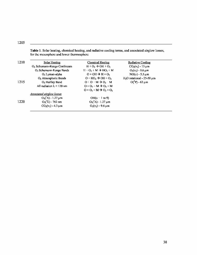
Table 1. Solar heating, chemical heating, and radiative cooling terms, and associated airglow losses,for the mesosphere and lower thermosphere

1205

1210 Solar HeatingO 2 Schumann-Runge Continuum

O2 Schumann-Runge BandsO2 Lyman-alpha

O2 Atmospheric Bands1215 O 3 Hartley Band

All radiation ), < 120 nm

Associated airglow losses

O2( 1 A) - 1.27 µm1220 O2( 1 E) - 762 nm

CO2(v3) - 4.3 µm

Chemical HeatingH + O 3 4 OH + O 2

H + O2 + M 4 HO 2 + MO + OH 4 H + O2

O + HO 2 4 OH + O 2

O + O + M 4 O2 + MO + O2 + M 4 O 3 + MO + O 3 + M 4 O2 + O2

OH(u = 1 to 9)O2( 1 A) - 1.27 µmO 3(v 3) – 9.6 µm

Radiative CoolingCO2(v2) - 15 µmO3(v3) - 9.6 µmNO(u) - 5.3 µm

H2O rotational - 25-50 µmO(3P) - 63 µm

38

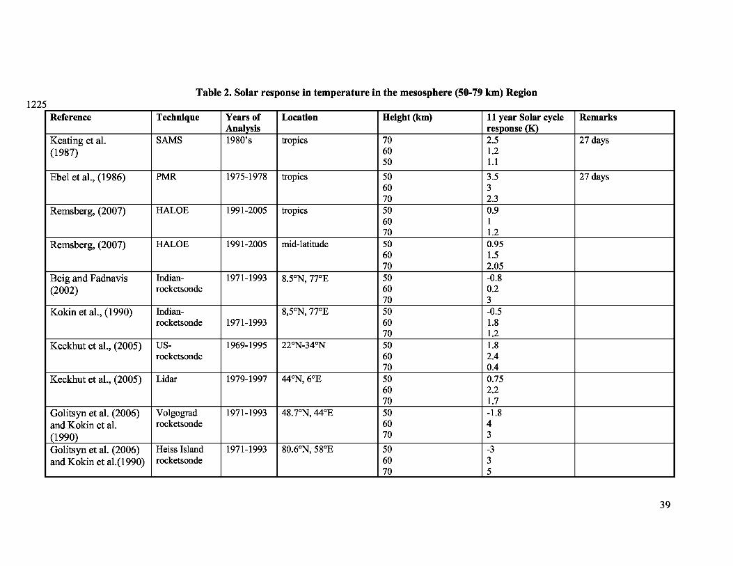
Table 2. Solar response in temperature in the mesosphere (50-79 km) Region1225

Reference Technique Years of Location Height (km) 11 year Solar cycle RemarksAnalysis response (K)

Keating et al. SAMS 1980’s tropics 70 2.5 27 days(1987) 60 1.2

50 1.1

Ebel et al., (1986) PMR 1975-1978 tropics 50 3.5 27 days60 370 2.3

Remsberg, (2007) HALOE 1991-2005 tropics 50 0.960 170 1.2

Remsberg, (2007) HALOE 1991-2005 mid-latitude 50 0.9560 1.570 2.05

Beig and Fadnavis Indian- 1971-1993 8.50N, 770 E 50 -0.8(2002) rocketsonde 60 0.2

70 3Kokin et al., (1990) Indian- 8,5°N, 77°E 50 -0.5

rocketsonde 1971-1993 60 1.870 1.2

Keckhut et al., (2005) US- 1969-1995 22°N-34°N 50 1.8rocketsonde 60 2.4

70 0.4Keckhut et al., (2005) Lidar 1979-1997 44°N, 6°E 50 0.75

60 2.270 1.7

Golitsyn et al. (2006) Volgograd 1971-1993 48.7°N, 44°E 50 -1.8and Kokin et al. rocketsonde 60 4

(1990) 70 3

Golitsyn et al. (2006) Heiss Island 1971-1993 80.6°N, 58°E 50 -3and Kokin et al.(1990) rocketsonde 60 3

70 5

39

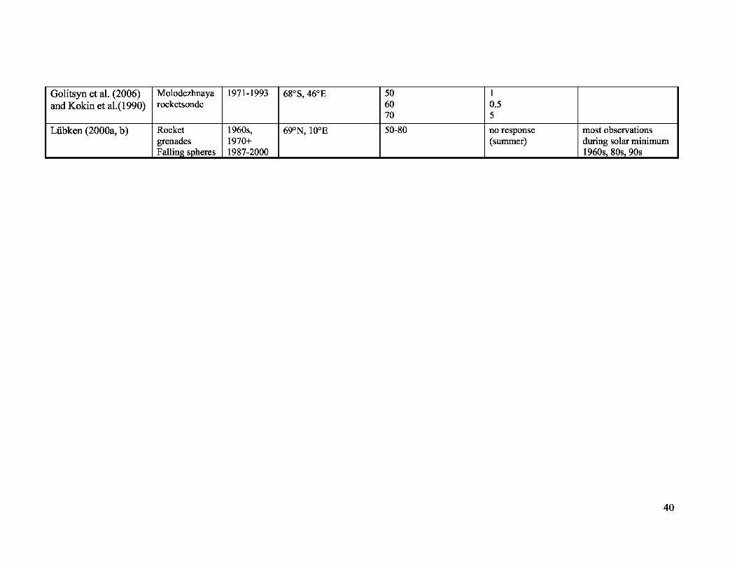
Golitsyn et al. (2006) Molodezhnaya 1971-1993 68°S, 46°E 50 1

and Kokin et al.(1990) rocketsonde 60 0.570 5

Lübken (2000a, b) Rocket 1960s, 69°N, 10°E 50-80 no response most observationsgrenades 1970+ (summer) during solar minimumFalling spheres 1987-2000 1960s, 80s, 90s

40

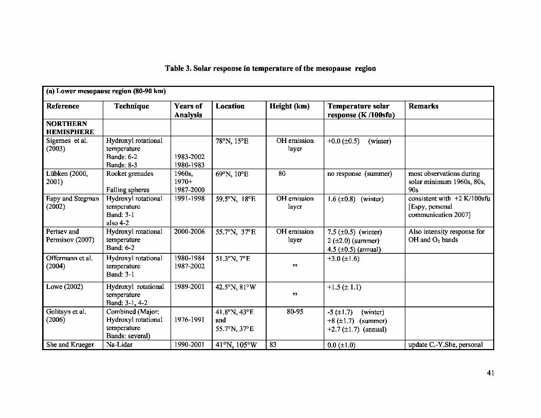
Table 3. Solar response in temperature of the mesopause region

(a) Lower mesopause region (80-90 km)

Reference Technique Years of Location Height (km) Temperature solar RemarksAnalysis response (K /100sfu)

NORTHERNHEMISPHERESigernes et al. Hydroxyl rotational 78°N, 15°E OH emission +0.0 (±0.5) (winter)(2003) temperature layer

Bands: 6-2 1983-2002Bands: 8-3 1980-1983

Lübken (2000, Rocket grenades 1960s, 69°N, 10°E 80 no response (summer) most observations during2001) 1970+ solar minimum 1960s, 80s,

Falling spheres 1987-2000 90sEspy and Stegman Hydroxyl rotational 1991-1998 59.5°N, 18° E OH emission 1.6 (±0.8) (winter) consistent with +2 K/100sfu(2002) temperature layer [Espy, personal

Band: 3-1 communication 2007]also 4-2

Pertsev and Hydroxyl rotational 2000-2006 55.7°N, 37° E OH emission 7.5 (±0.5) (winter) Also intensity response forPerminov (2007) temperature layer 2 (±2.0) (summer) OH and O2 bands

Band: 6-2 4.5 (±0.5) (annual)Offermann et al. Hydroxyl rotational 1980-1984 51.3°N, 7° E +3.0 (± 1.6)(2004) temperature 1987-2002 ”

Band: 3-1

Lowe (2002) Hydroxyl rotational 1989-2001 42.5°N, 8 1 ° W +1.5 (± 1.1)temperature ”Band: 3-1, 4-2

Golitsyn et al. Combined (Major: 41.8°N, 43° E 80-95 -5 (± 1.7) (winter)(2006) Hydroxyl rotational 1976-1991 and +8 (± 1.7) (summer)

temperature 55.7°N, 37° E +2.7 (± 1.7) (annual)Bands: several)

She and Krueger Na-Lidar 1990-2001 41°N, 105°W 83 0.0 (± 1.0) update C.-Y.She, personal

41

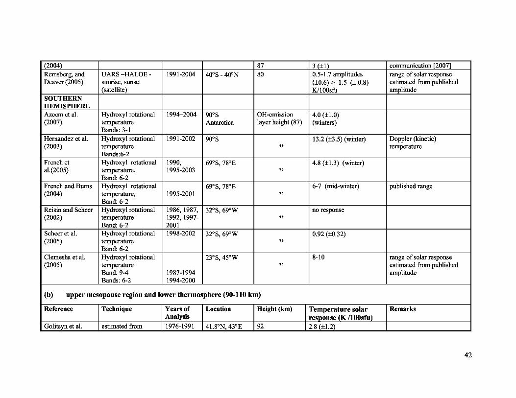
(2004) 87 3 (±1) communication [2007]Remsberg, and UARS –HALOE - 1991-2004 40°S - 40°N 80 0.5-1.7 amplitudes range of solar responseDeaver (2005) sunrise, sunset (±0.6)-> 1.5 (±.0.8) estimated from published

(satellite) K/100sfu amplitudeSOUTHERNHEMISPHEREAzeem et al. Hydroxyl rotational 1994–2004 90°S OH-emission 4.0 (±1.0)(2007) temperature Antarctica layer height (87) (winters)

Bands: 3-1Hernandez et al. Hydroxyl rotational 1991-2002 90°S 13.2 (±3.5) (winter) Doppler (kinetic)(2003) temperature » temperature

Bands:6-2French et Hydroxyl rotational 1990, 69°S, 78°E 4.8 (±1.3) (winter)al.(2005) temperature, 1995-2003 »

Band: 6-2French and Burns Hydroxyl rotational 69°S, 78°E 6-7 (mid-winter) published range(2004) temperature, 1995-2001 »

Band: 6-2Reisin and Scheer Hydroxyl rotational 1986, 1987, 32°S, 69°W no response(2002) temperature 1992, 1997- »

Band: 6-2 2001Scheer et al. Hydroxyl rotational 1998-2002 32°S, 69°W 0.92 (±0.32)(2005) temperature »

Band: 6-2Clemesha et al. Hydroxyl rotational 23°S, 45°W 8-10 range of solar response(2005) temperature » estimated from published

Band: 9-4 1987-1994 amplitudeBands: 6-2 1994-2000

(b) upper mesopause region and lower thermosphere (90-110 km)

Reference Technique Years of Location Height (km) Temperature solar RemarksAnalysis response (K /100sfu)

Golitsyn et al. estimated from 1976-1991 41.8°N, 43°E 92 2.8 (±1.2)

42

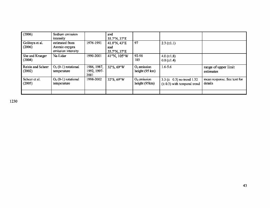
(2006) Sodium emission andintensity 55.7°N, 37° E

Golitsyn et al. estimated from 1976-1991 41.8°N, 43° E 97 2.3 (±1.1)(2006) Atomic oxygen and

emission intensity 55.7°N, 37° EShe and Krueger Na-Lidar 1990-2001 41 °N, 105 °W 92-98 4.0 (± 1.8)(2004) 103 0.0 (±1.4)

Reisin and Scheer O2 (0-1) rotational 1986, 1987, 32° S, 69°W O2 emission 1.6-5.6 range of upper limit(2002) temperature 1992, 1997- height (95 km) estimates

2001Scheer et al. O2 (0-1) rotational 1998-2002 32° S, 69° W O2 emission 3.3 (± 0.3) no trend 1.32 mean response. See text for(2005) temperature height (95km) (± 0.3) with temporal trend details

1230

43

* `*

;

**

------------ ------ ------------------

** ** **

* ***

----- ------ ;----------- -- -----`

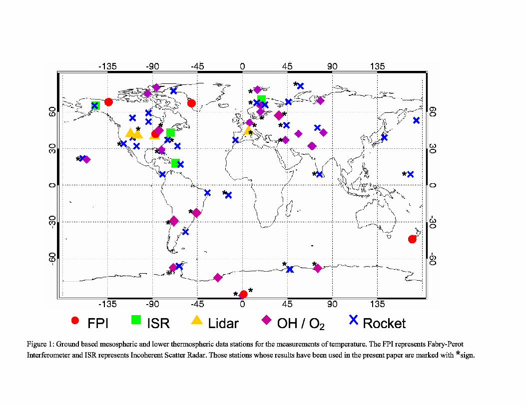
* x* *

'--'--'-'------'--'------------------r'-- ------------ ............-'-"

*.... --- ------------- ---------- -- ------- -- - - c -- - - - - - - - - - - - - - - - -'

'^ n.

*--------------------------------------- ---- *----- ---------------------------- ----- ----------------------------------------------------------------

3

*L-1 *.

* *

• FPI ISR \ Lidar OH / O2 RocketFigure 1: Ground based mesospheric and lower thermospheric data stations for the measurements of temperature. The FPI represents Fabry-PerotInterferometer and ISR represents Incoherent Scatter Radar. Those stations whose results have been used in the present paper are marked with *sign.

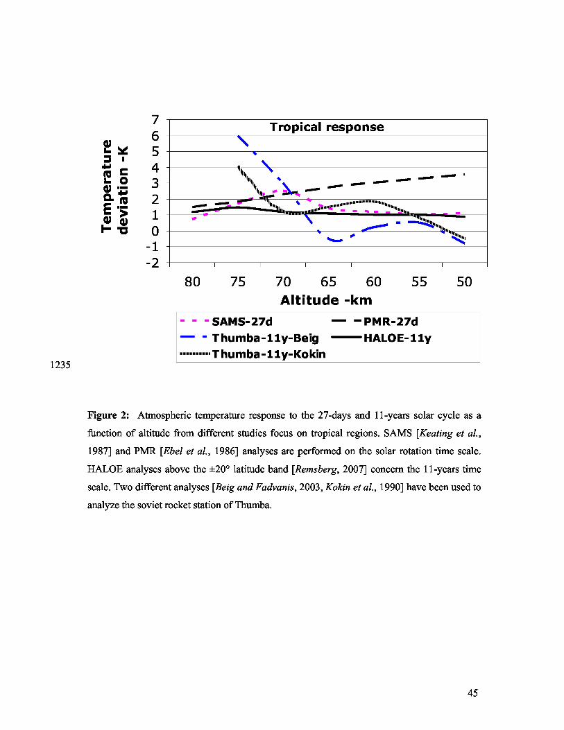
7

65

4321

0-1

-2

Tropical response

n npnn _i

^ - ^ °̂nm^ h nul

^ °Humana

80 75 70 65 60 55 50

Altitude -km

- - - SAMS-27d — – PMR-27d

Thumba-11y-Beig HALOE-11y

Thumba-11y-Kokin

Figure 2: Atmospheric temperature response to the 27-days and 11-years solar cycle as a

function of altitude from different studies focus on tropical regions. SAMS [ Keating et al.,

1987] and PMR [Ebel et al., 1986] analyses are performed on the solar rotation time scale.

HALOE analyses above the ±20° latitude band [Remsberg, 2007] concern the 11-years time

scale. Two different analyses [Beig and Fadvanis, 2003, Kokin et al., 1990] have been used to

analyze the soviet rocket station of Thumba.

1235

45

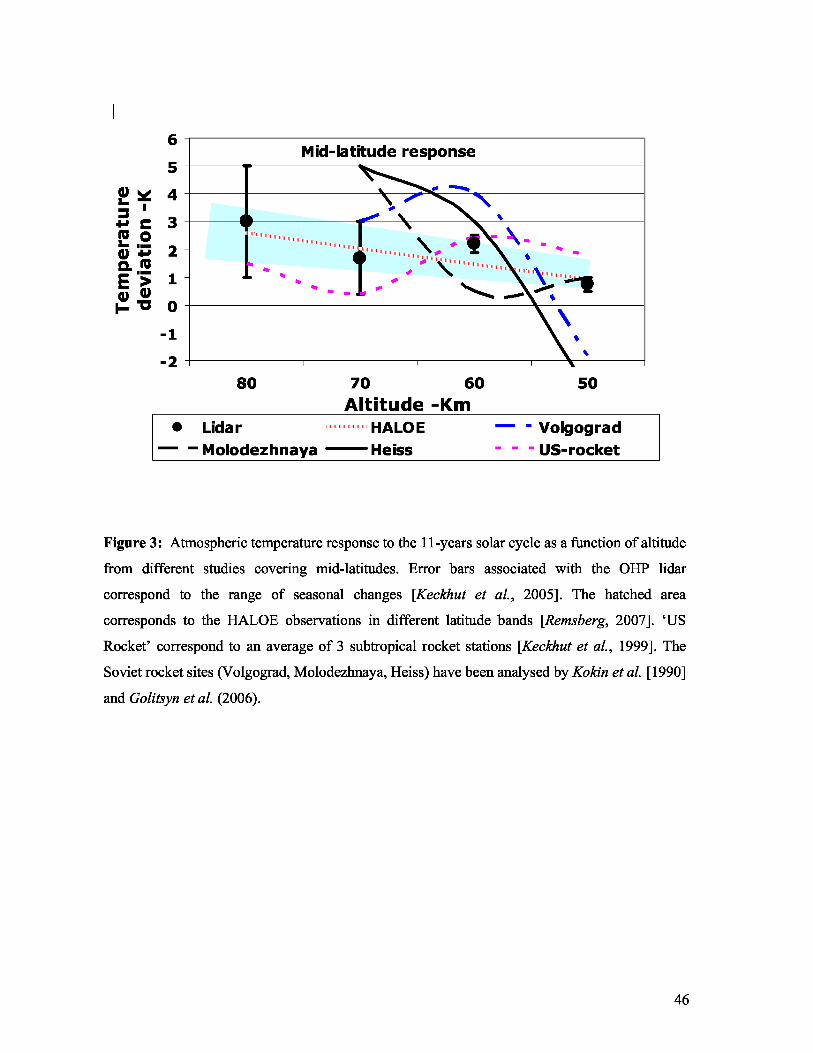
5

i 4

C 3

*+ 2C. ME 3P 1

H '^ 0

-1

-2

6Mid-latitude response

80 70 60 50

Altitude -Km• Lidar HALOE — - Volgograd

— – Molodezhnaya Heiss - - - US-rocket

Figure 3: Atmospheric temperature response to the 11-years solar cycle as a function of altitude

from different studies covering mid-latitudes. Error bars associated with the OHP lidar

correspond to the range of seasonal changes [ Keckhut et al., 2005]. The hatched area

corresponds to the HALOE observations in different latitude bands [Remsberg, 2007]. ‘US

Rocket’ correspond to an average of 3 subtropical rocket stations [ Keckhut et al., 1999]. The

Soviet rocket sites (Volgograd, Molodezhnaya, Heiss) have been analysed by Kokin et al. [ 1990]

and Golitsyn et al. (2006).

46

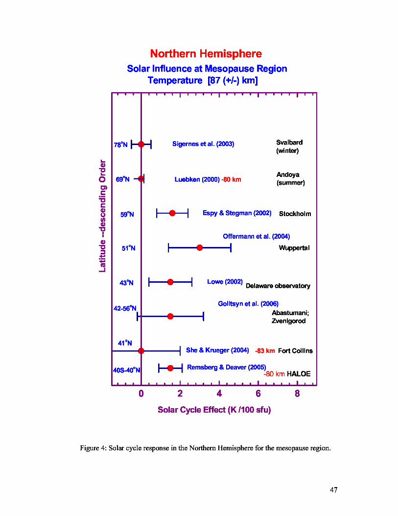
Northern HemisphereSolar Influence at Mesopause Region

Temperature [87 (+/-) km]

78oN Sigernes et al. (2003) Svalbard(winter)

69oNLuebken (2000) -80 kmAndoya

—+ (summer)

59oN I I--♦^ Espy & Stegman (2002) Stockholm

Offermann et al. (2004)

51 oN Wuppertal

43oN Lowe (2002) Delaware observatory

42-56oN Golitsyn et al. (2006)

Abastumani;Zvenigorod

41oNShe & Krueger (2004) -83 km Fort Collins

40S-40oN ^--^^ Remsberg & Deaver (2005)-80 km HALOE

0 2 4 6 8

Solar Cycle Effect (K /100 sfu)

Figure 4: Solar cycle response in the Northern Hemisphere for the mesopause region.

47

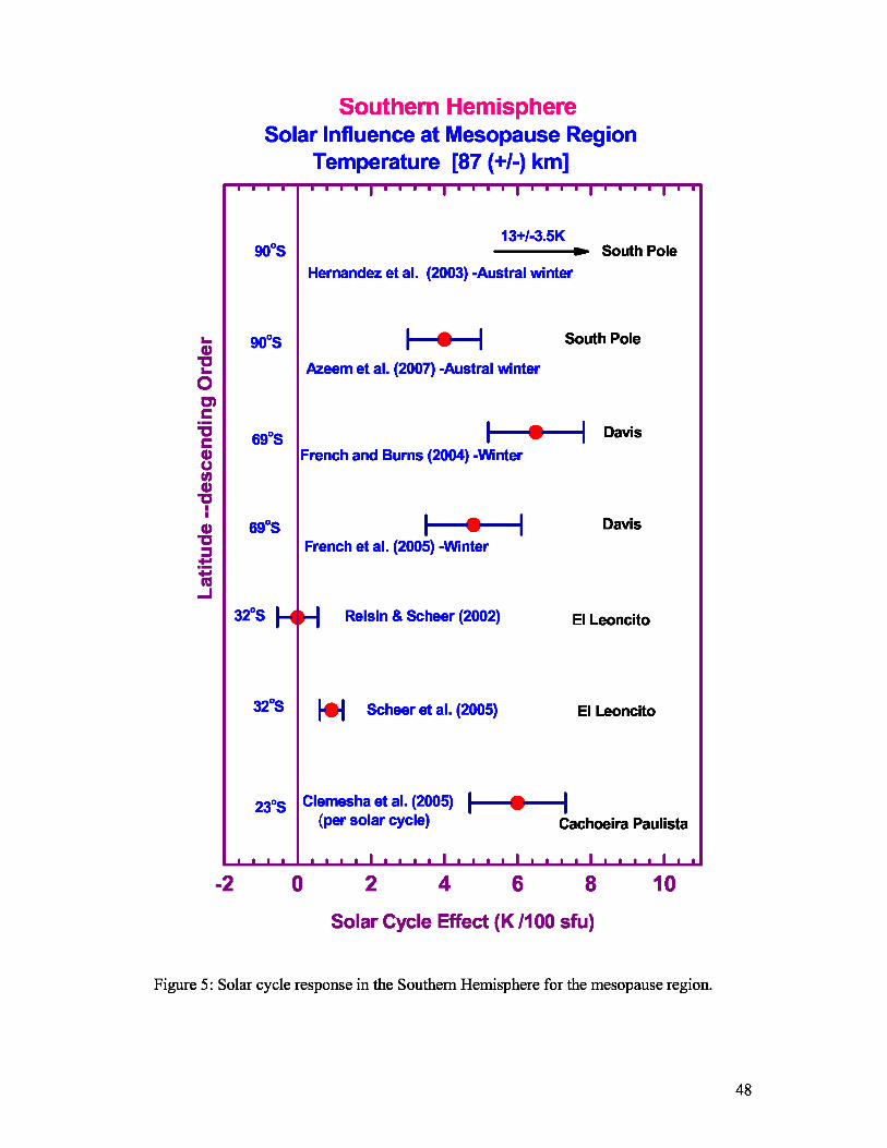
Southern HemisphereSolar Influence at Mesopause Region

Temperature [87 (+/-) km]

13+/-3.5K90oSSouth Pole

Hernandez et al. (2003) -Austral winter

90oS

South Pole

Azeem et al. (2007) -Austral winter

69oS

DavisFrench and Burns (2004) -Winter

69oS

DavisFrench et al. (2005) -Winter

32oS ^-^ Reisin & Scheer (2002) El Leoncito

32oS I [* Scheer et al. (2005) El Leoncito

23oS I Clemesha et al. (2005)(per solar cycle) Cachoeira Paulista

-2 0 2 4 6 8 10

Solar Cycle Effect (K /100 sfu)

Figure 5: Solar cycle response in the Southern Hemisphere for the mesopause region.

48

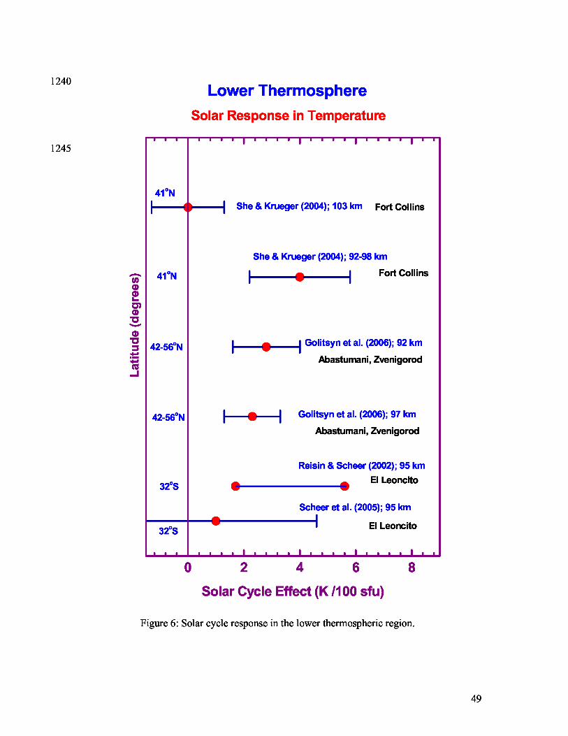
1240Lower Thermosphere

Solar Response in Temperature

1245

41oNShe & Krueger (2004); 103 km Fort Collins

She & Krueger (2004); 92-98 km

41oN

Fort Collins

1 42-56oN Golitsyn et al. (2006); 92 km

Abastumani, Zvenigorod

42-56oN Golitsyn et al. (2006); 97 km

Abastumani, Zvenigorod

Reisin & Scheer (2002); 95 km

32oS

40 0El Leoncito

Scheer et al. (2005); 95 km

32oS El Leoncito

0 2 4 6 8

Solar Cycle Effect (K /100 sfu)

Figure 6: Solar cycle response in the lower thermospheric region.

49