Overview of Mathematical Tools for Intermediate Microeconomics

Christopher FlinnDepartment of EconomicsNew York University

August 2002

Copyright c° 2002 Christopher FlinnAll Rights Reserved

Contents

1 Functions 2

2 Limits 2

3 Derivatives of a Univariate Function 5

4 Some Rules of Differentiation 9

5 Maximization and Minimization of Univariate Functions 9

6 Multivariate Functions 12

7 Partial Derivatives of Multivariate Functions 14

8 Total Derivatives 17

9 Maximization and Minimization of Multivariate Functions 19

10 Some Important Functions for Economists 2310.1 Linear . . . . . . . . . . . . . . . . . . . . . . . . . . . . . . . . . . . . . . . . . . . . 2310.2 Fixed Coefficients . . . . . . . . . . . . . . . . . . . . . . . . . . . . . . . . . . . . . . 2310.3 Cobb-Douglas . . . . . . . . . . . . . . . . . . . . . . . . . . . . . . . . . . . . . . . . 2410.4 Quasi-Linear . . . . . . . . . . . . . . . . . . . . . . . . . . . . . . . . . . . . . . . . 25

1

Economics is a quantitative social science and to appreciate its usefulness in problem solvingrequires us to make limited use of some results from the differential calculus. These notes are toserve as an overview of definitions and concepts that we will utilize repeatedly during the semester,particularly in the process of solving problems and in the rigorous statements of concepts anddefinitions.

1 Functions

Central to virtually all economic arguments is the notion of a function. For example, in the studyof consumer choice we typically begin the analysis with the specification of a utility function,from which we later derive a system of demand functions, which can be used in conjunction withthe utility function to define an indirect utility function. When studying firm behavior, we workwith production functions, from which we define (many types of) cost functions, factor demandfunctions, firm supply functions, and industry supply functions. You get the idea - functions arewith us every step of the way, whether we use calculus or simply graphical arguments in analyzingthe problems we confront in economics.

Definition 1 A univariate (real) function is a rule associating a unique real number y = f(x) witheach element x belonging to a set X.

Thus a function is a rule that associates, for every value x in some set X, a unique outcomey. The particularly important characteristic that we stress is that there is a unique value of yassociated with each value of x. There can, in general, be different values of x that yield the samevalue of y however. When a function also has the property that for every value of y there exists aunique value of x we say that the function is 1-1 or invertible.

Example 2 Let y = 3 + 2x. For every value of x there exists a unique value of y, so that this isclearly a function. Note that it is also an invertible function since we can write

y = 3 + 2x

⇒ x =y − 32.

Thus there exists a unique value of y for every value of x.

Example 3 Let y = x2. As required, for every value of x there exists a unique value of y. Howeverfor every positive value of y there exists two possible values of x given by

√y and -

√y. Hence this

is a function, but not an invertible one.

2 Limits

Let a function f(x) be defined in terms of x. We say that the limit of the function as x becomesarbitrarily close to some value x0 is A, or

limx→x0

f(x) = A.

2

Technically this means that for any ε > 0 there exists a δ such that

|x− x0| < δ ⇒ |f(x)−A| < ε,

where |z| denotes the absolute value of z (i.e. |z| = z if z ≥ 0 and |z| = −z if z < 0).The limit of a function at a point x0 need not be equal to the value of the function at that

point, that islimx→x0

f(x) = A

does not necessarily imply thatf(x0) = A.

In fact, it may be that f(x0) is not even defined.

Example 4 Let y = f(x) = 3+2x. Then as x→ 3, y → 9, or the limit of f(x) = 9 as x→ 3. Thisis shown by demonstrating that |f(x)− 9| < ε for any ε if |x− 3| is sufficiently small. Note that

|f(x)− 9| = |3 + 2x− 9|= |2x− 6| = 2|x− 3|.

If we choose δ = ε/2, then if |x− 3| < δ,

2|x− 3| = |2x− 6| = |f(x)− 9| < 2δ = ε.

Thus for any ε, no matter how small, by setting δ = ε/2, |x − 3| < δ implies that |f(x) − 9| < ε.Then by definition

limx→3 f(x) = 9.

It so happens that in this casef(3) = 9,

but these are not the same thing.

Definition 5 When limx→x0 f(x) = f(x0) we say that the function is continuous at x0.

Then our example f(x) = 3 + 2x is continuous at the value x0 = 3. You should be able toconvince yourself that this function is continuous everywhere on the real line R ≡ (−∞,∞). Anexample of a function that is not continuous everywhere on R is the following.

Example 6 Let the function f be defined as

f(x) =

(x2 if x 6= 01 if x = 0

.

First, consider the limit of f(x) for any point not equal to 0, say for example at x = 2. Nowf(2) = 4. For any ε > 0, |f(x)− 4| < ε is equivalent to |x2− 4| < ε, or |x− 2||x+2| < ε. At pointsnear x = 2, |x + 2| → 4. It is clearly the case that |x + 2| < 5, say, for x sufficiently close to 2.Then let δ = ε/5. Then |x − 2| < δ implies that ε > 5|x − 2| > |x + 2||x − 2| = |f(x) − 4|. Thusthere exists a δ (in this case we have chosen δ = ε/5) such that if x is within δ of x0 = 2 (that is,|x− 2| < δ), then f(x) is within ε of the value 4, and this holds for any choice of ε. We also notethat since f(2) = 4, the function is continuous at 2.

3

We note that the function is continuous in this example is continuous at all points other thanx0 = 0. To see this, note the following.

Example 7 (Continued) The limit of f(x) at 0 is given by

limx→0 f(x) = 0.

This is the case because for any arbitrary ε > 0 there exists a δ > 0 such that |x| < δ implies that|x2 − 0| < ε. However, since f(0) = 1, we have

limx→0 f(x) 6= f(0),

so that the function is not continuous at the point x0 = 0. As we remarked above, it is continuouseverywhere else on R.

On an intuitive level, we say that a function is continuous if the function can be drawn withoutever lifting one’s pencil from the sheet of paper. In Example 4 the function was a straight line,and this function obviously can be drawn without ever lifting one’s pencil (although it would takea long time to draw the line since it extends indefinitely in either direction). On the other hand,in Example 6 we have to lift our pencil at the value x = 0, where we have to move up to plot thepoint f(0) = 1. Thus this function is not continuous at that one point.

To rigorously define continuity, and, in the next section, differentiability, it will be useful tointroduce the concepts of the left hand limit and the right hand limit. These are only distinguishedby the fact that the left hand limit of the function at some point x0 is defined by taking increasinglarge values of x that become arbitrarily close to x0, while the right hand limit of the function isobtained by taking increasingly smaller values of x that become arbitrarily close to the point x0.Up to this point we have been describing the limiting operation implicitly in terms of the righthand limit. Now let’s explicitly distinguish between the two.

Definition 8 Let ∆x > 0. At a point x0 the left hand limit of the function f is defined as

L1(x0) = lim∆x→0

f(x0 −∆x),

and the right hand limit is defined as

R1(x0) = lim∆x→0

f(x0 +∆x).

We then have the following result.

Definition 9 A function f is continuous at the point x0 if and only if

L1(x0) = R1(x0) = f(x0).

We say that the function is continuous everywhere on its domain if L1(x) = R1(x) for all x inthe domain of f.

4

3 Derivatives of a Univariate Function

Armed with the definition of a function, continuity, and limits, we have all the ingredients to definethe derivatives of a univariate function. A derivative is essentially just the rate of a change of afunction evaluated at some point. The section heading speaks of derivatives in the plural since wecan speak of the rate of change of the function itself (first derivative), the rate of change of the rateof change of the function (the second derivative), etc. Don’t become worried, we shall never needto use anything more than the second derivative in this course (and that rarely).

Consider a function f(x) which is continuous at the the point x0. We can of course “perturb”the value of x0 by a small amount, let’s say by ∆x. ∆x could be positive or negative, but withoutany loss of generality let’s say that it is positive. Thus the “new” value of x is x0 plus the change,or x0+∆x. Now we can consider how much the function changes when we move from the point x0to the point x0 +∆x. The function change is given by

∆y = f(x0 +∆x)− f(x0).Thus the rate of change (or average change) in the function is given by

∆y

∆x=f(x0 +∆x)− f(x0)

∆x.

Definition 10 The (first) derivative of the function f(x) evaluated at the point x0 is defined asthis rate of change as the perturbation ∆x becomes arbitrarily small, or

dy

dx

¯̄̄̄x=x0

= lim∆x→0

f(x0 +∆x)− f(x0)∆x

. (1)

For [1] to be well-defined requires that the function f have certain properties at the pointx0. First, it must be continuous at x0, but in addition must have the further property that itbe differentiable at x0. For the function f to be differentiable at x0 requires that the operationdescribed on the right hand side of [1] be the same whether the point x0 is approached from “theleft” or from “the right.” Say that ∆x is always positive, which is the convention we have adopted.Then the limit represented on the right hand side of [1] represents the limit of the quotient fromthe right (taking successively smaller values of ∆x but such that x0 +∆x is always greater thanx0). The left hand limit can be defined as

L2(x0) = lim∆x→0

f(x0 −∆x)− f(x0)∆x

,

and the right hand limit can be defined as

R2(x0) = lim∆x→0

f(x0 +∆x)− f(x0)∆x

.

Then we have the following definition of differentiability at the point x0.

Definition 11 The function f is (first order) differentiable at the point x0 in its domain if andonly if L2(x0) = R2(x0).

5

We say that the function f is (first order) differentiable everywhere on its domain if L2(x) =R2(x) for all points x in its domain.

Example 12 Consider the function

f(x) =

(0 if x < 2

x− 2 if x ≥ 2 .

We first note that this function is continuous everywhere on R. Now consider the derivative of thisfunction at the point x0 = 2. The left hand derivative would be defined as

lim∆x→0

f(2−∆x)− f(2)∆x

= lim∆x→0

0− 0∆x

= 0.

The right hand side derivative at the point x0 = 2 would instead be

lim∆x→0

f(2 +∆x)− f(2)∆x

= lim∆x→0

∆x

∆x= 1.

Thus the left hand side and right hand side derivatives are different at the point x0 = 2, and so thefunction is not differentiable there. You should convince yourself that this function is differentiableat every other point in R, however.

For functions f that are differentiable at a point x0, we can now consider some examples of thecomputation of first derivatives.

Example 13 (Quadratic function) Let f(x) = a + bx + cx2, where a, b, and c are fixed scalars.This function is everywhere differentiable on the real line R. Let’s consider the computation of thederivative of f at the point x0 = 2. Then we have

dy

dx

¯̄̄̄x=2

= lim∆x→0

f(2 +∆x)− f(2)∆x

= lim∆x→0

[a+ b(2 +∆x) + c(2 +∆x)2]− [a+ b2 + c22]∆x

= lim∆x→0

b∆x+ 4c∆x+ c(∆x)2

∆x

= b+ 4c+ lim∆x→0

c(∆x)2

∆x

= b+ 4c+ c lim∆x→0

(∆x)2

∆x= b+ 4c.

[Note: Convince yourself that lim∆x→0(∆x)n

∆x = 0 for all n > 1.]

6

Example 14 (General polynomial) Let f(x) = xn. Then

dy

dx

¯̄̄̄x= lim

∆x→0(x+∆x)n − xn

∆x

= lim∆x→0

[xn + nxn−1∆x+ n(n−1)2 xn−2(∆x)2 + ...]− xn∆x

= lim∆x→0

[nxn−1∆x+ n(n−1)2 xn−2(∆x)2 + n(n−1)(n−2)

6 xn−3(∆x)3 + ...]∆x

= lim∆x→0

nxn−1∆x∆x

+ lim∆x→0

n(n− 1)xn−2(∆x)2∆x

+ lim∆x→0

n(n− 1)(n− 2)xn−3(∆x)3∆x

+ ...

= nxn−1 + 0 + 0 + ... .

This last line follows from the fact that

lim∆x→0

(∆x)r

(∆x)= 0, r > 1.

Differentiation is a linear operation. That means that if our function is modified to include amultiplicative constant k, the derivative of the new function is

d(kxn)

dx= knxn−1.

By the same token, if we define another polynomial function, for example

g(x) = lxm,

then the derivative of the function

f(x) + g(x) = kxn + lxm

is just the sum of the derivatives of each, or

d(f(x) + g(x))

dx=

df(x)

dx+dg(x)

dx= knxn−1 + lmxm−1.

Using this result we see that the derivative of

f(x) = 6x4 + 3x2 − 1.5x+ 2

is

f 0(x) ≡ df(x)dx

= 24x3 + 6x− 1.5.

7

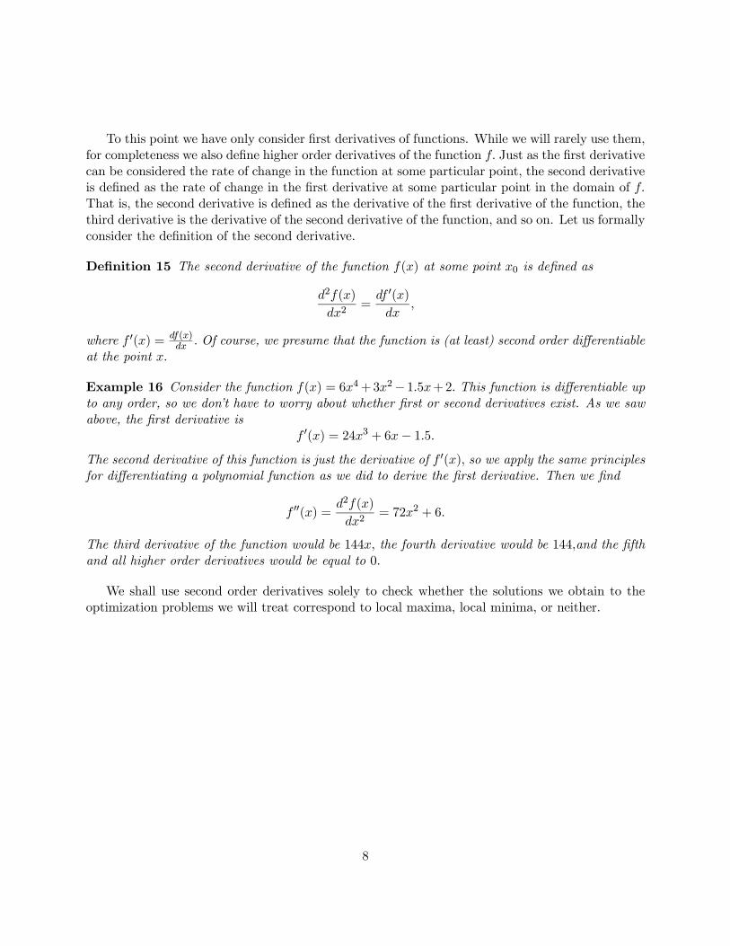
To this point we have only consider first derivatives of functions. While we will rarely use them,for completeness we also define higher order derivatives of the function f. Just as the first derivativecan be considered the rate of change in the function at some particular point, the second derivativeis defined as the rate of change in the first derivative at some particular point in the domain of f.That is, the second derivative is defined as the derivative of the first derivative of the function, thethird derivative is the derivative of the second derivative of the function, and so on. Let us formallyconsider the definition of the second derivative.

Definition 15 The second derivative of the function f(x) at some point x0 is defined as

d2f(x)

dx2=df 0(x)dx

,

where f 0(x) = df(x)dx . Of course, we presume that the function is (at least) second order differentiable

at the point x.

Example 16 Consider the function f(x) = 6x4+3x2− 1.5x+2. This function is differentiable upto any order, so we don’t have to worry about whether first or second derivatives exist. As we sawabove, the first derivative is

f 0(x) = 24x3 + 6x− 1.5.The second derivative of this function is just the derivative of f 0(x), so we apply the same principlesfor differentiating a polynomial function as we did to derive the first derivative. Then we find

f 00(x) =d2f(x)

dx2= 72x2 + 6.

The third derivative of the function would be 144x, the fourth derivative would be 144,and the fifthand all higher order derivatives would be equal to 0.

We shall use second order derivatives solely to check whether the solutions we obtain to theoptimization problems we will treat correspond to local maxima, local minima, or neither.

8

4 Some Rules of Differentiation

In this section we simply list some of the most common rules of differentiation that you are likelyto need this semester. For completeness, the list includes a few that won’t be used as well. Wewill discuss derivatives of the functions that we will most commonly encounter in the last sectionof this handout.

In the following expressions a and n represent constants while f(x) and g(x) are unspecified(differentiable) functions of the single variable x.

1. ddx(a) = 0.

2. ddx(x) = 1.

3. ddx(ax) = a.

4. ddx(f(x) + g(x)) =

ddx(f(x)) +

ddx(g(x))

5. ddx(f(x)g(x)) = f(x)

dg(x)dx + g(x)df(x)dx .

6. ddx(

f(x)g(x) ) =

1g(x)

df(x)dx − f(x)

g(x)2dg(x)dx

7. ddx(f(x))

n = (n− 1)f(x)n−1 df(x)dx

8. ddx(f(g(x)) =

ddg(x)(f(g(x))) · ddx(g(x)) (Chain Rule)

9. ddx(ln f(x)) =

1f(x)

ddx(f(x))

10. ddx(exp(f(x))) = exp(f(x)) · ddx(f(x)).

Note that in equation 9 the symbol “ ln ” represents logarithm to the base e, where e is the nat-ural number approximately equal to 2.718. Similarly, in expression 10 the symbol “exp ” representse, and signifies the the term following is the exponent of e. That is, exp(x) = ex.

These derivative expressions are all that you will be using in this course, and for that matterrepresent those relationships most frequently used in performing applied economics at any level.

5 Maximization and Minimization of Univariate Functions

In this Section we introduce the idea of maximization and minimization of functions of one variable.We only consider unconstrained optimization (the term “optimization” encompasses maximizationand minimization) here to introduce ideas. The main tool of applied economics is constrainedoptimization of multivariate functions, a topic treated below. We will only very quickly introducethe subject and will skip over most details. The development is decidedly nonrigorous and onlytreats special cases likely to be of interest to us in this course.

Let f(x) be a univariate function of x, and assume that x is differentiable everywhere on itsdomain (which let’s assume is the entire real line, denote by R). Let’s introduce the subject byconsidering some simple examples.

9

Example 17 Let us consider finding the value of x that maximizes the function f(x) = 2x. Now thefirst derivative of this function is d(2x)/dx = 2. This means that for every unit that x is increasedthe function is increased by 2 units. Clearly the maximum of the function is obtained by taking x tobe as large as possible. This is an example in which the maximization (or minimization) problemis not well-posed since the solution to the problem is not finite.

Example 18 Consider the maximization of the function g(x) = 5 + x − 2x2. In maximizing thisfunction we don’t run into the same problem as we had in the case of f(x) = 2x, since clearly asx gets indefinitely large or indefinitely small (x→ −∞) the function g(x) goes to −∞ as well. InFigure 1.a we plot the function and you can note its behavior. In Figure 1.b we plot the derivativeof the function as well. We observe the following behavior. There exists one maximum value of thefunction, and this value is equal to 5.125, and the value of x that is associated with the maximumfunction value is equal to .25.

We note that at the value of x = .25 the derivative of the function is 0. To the left of that value,i.e., for x < .25, the derivative of the function is positive, which indicates that by increasing x wecan increase the function value. To the right of .25, i.e., for values of x > .25 the derivative isnegative, indicating that further increases in x decrease the function value. Then the value of xthat maximizes the function is that value at which the derivative of the function is 0.

Say that a function f(x) is continuously differentiable on some interval D, where D could bethe entire real line. Let’s say that we are attempting to locate the global maximum of f, where bythe global maximum we mean that there exists an x∗ (assume it is unique) such that f(x∗) > f(y)for all y ∈ D, y 6= x∗. The function f can also possess local maxima (the point x∗ will always bea local as well as a global maximum). A local maximum is defined as follows. Consider a point x̂.Then x̂ is a local maximum if f(x̂) > f(z), z ∈ (x̂ − ε1, x̂ + ε2), z 6= x̂, for some ε1 > 0, ε2 > 0,(x̂− ε1, x̂+ ε2) ⊆ D.

On the intervalD, let’s define the set of points E = {τ1, ..., τm} such that the following conditionholds

f 0(τ i) ≡ df(x)

dx

¯̄̄̄τ i

= 0, i = 1, ...,m.

Since f is continuously differentiable, it also possesses second derivatives. Consider the set of secondderivatives of f evaluated at the points (τ1, ..., τm),

{f 00(τ1), ..., f 00(τm)}.Condition 19 The set of points E1 ⊆ E such that

x ∈ E1 ⇔ f 00(x) < 0

contains all of the local maxima of f on the interval D.

Condition 20 The set of points E2 ⊆ E such that

x ∈ E2 ⇔ f 00(x) > 0

contains all of the local minima of f on the interval D.

10

Condition 21 The set of points E3 ⊆ E such that

x ∈ E2 ⇔ f 00(x) = 0

contains all of the inflection points of f on the interval D.

Clearly the sets E1, E2, and E3 contain no points in common and E1 ∪ E2 ∪ E3 = E (i.e., E1,E2, and E3 constitute a partition of E).

The conditions presented above are extremely useful ones in practice. It is often the case thatthe functions we work with in economic applications are very well-behaved - that is the reasonwe choose to work with them. For example, if we work with a quadratic function of x defined onthe entire real line we know immediately that the function will either possess (1) a unique, finitemaximum and no finite minimum or (2) a unique, finite minimum and no finite maximum. To seethis, write the “general” form of the quadratic function as

f(x) = a+ bx+ cx2,

where a, b, and c are scalars that can be of any sign, but we require that b 6= 0 and c 6= 0. Beginby defining the set of values {τ1, ..., τm} of this function where the first derivative is 0. Note that

f 0(x) = b+ 2cx,

and now find the values of x where this function is equal to 0. It is clear that there is only onevalue of x that solves this equation, so that m = 1. The solution is

τ1 = − b2c.

The second derivative of the function evaluated at τ1 is

f 00(τ1) = 2c.

Thus τ1 corresponds to a maximum if and only if c < 0. It corresponds to a minimum when c > 0.In either case, since there is only one element of E, the extreme point located is unique.

Say that the function to be maximized is quadratic and that c > 0. In this case we know thatf possesses one global minimum value on R, and the value at which the minimum is obtained isequal to −b/2c. What about the maximum value attained by this function? Clearly, as x becomesindefinitely large the value of f becomes indefinitely large (since the term cx2 will eventually“dominate” the term bx in determining the function value no matter what the sign or absolutesize of b). In this case we say that the function is unbounded on R, and there exists no value of xthat yields the maximum function value. We’ll say in this case that the maximum of the functiondoesn’t exist.

For some functions, like the one we will look at in the next example, there can exist multiplelocal maxima and/or minima, i.e., the sets E1 and or E2 contain more than one element. Say thatwe are interested in locating the global maximum of the function f and the set E1 contains morethan one element. The only way to accomplish the task is the “brute force” method of evaluating

11

the function at each of the elements of E1 and then define the global maximum as that element ofE1 associated with the largest function value. Formally, x∗ is the global maximum if x∗ ∈ E1 and

f(x∗) > f(y), all y ∈ E1, y 6= x∗.

The global minimum is analogously defined.

Example 22 Let us attempt to locate the global maximum and minimum of the cubic equation

f(x) = a+ bx+ cx2 + dx3.

Now the first order condition is

f 0(τ i) = 0 = b+ 2cτ i + 3dτ2i .

This is a quadratic equation, and therefore it has two solutions, which are given by

τ∗1 =−2c+√4c2 − 12bd

2b; τ∗1 =

−2c−√4c2 − 12bd2b

.

Both solutions will be real numbers if 4c2 > 12bd, and let us suppose that this is the case.Now to see whether the solutions correspond to local maxima, local minima, or inflection points

we have to evaluate the second derivatives of the function at τ∗1 and τ∗2. As long as both solutions arereal, then the second derivative of the function evaluated at one of the solutions will be positive andthe other negative. Therefore, the maximum of the function and the minimum of the function wouldappear to be unique. This is only apparently true however, since if the domain of the function is R,there is no finite maximum of minimum. Since as x gets large the function is dominated by the termdx3, if d > 0, for example, the function becomes indefinitely large as x→∞ and becomes indefinitelysmall as x → −∞. Thus the first order conditions determine the maximum and minimum of thefunction only if the domain of the function D is restricted appropriately. See the associated figurefor the details.

6 Multivariate Functions

A multivariate function is identical to a univariate function except for the fact that it has morethan one “argument.” In our course we will begin by studying consumer theory, and virtuallyalways we will deal with the case in which an individual’s “utility” is determined by their level ofconsumption of two goods, say x1 and x2. We will write this as

u = U(x1, x2),

where U is the utility function and u denotes the level of utility the consumer attains when con-suming the level x1 of the first good and x2 of the second. When we assert that U is a function,we mean that for each pair of values (x1, x2) there exists one and only one value of the function U,that is, the quantity u is unique for each pair of values (x1, x2).

12

In general a multivariate function is defined with respect to n arguments as

y = f(x1, x2, ..., xn),

where n is a positive integer greater than 1. Thus we could define our utility function over n goodsinstead of 2, which would make our analysis more “realistic,” without question, but complicatesthings and doesn’t add any insights at the level of analysis we will be operating in this course.

When we work with multivariate functions we will often be interested in the relationship betweenthe outcome measure y and one of the arguments of the function holding the other argument (orarguments) of the function fixed at some given values. By holding all other arguments fixed atsome preassigned values, the function becomes a univariate one since only one of the arguments isallowed to freely vary.

Example 23 Consider the linear combination of x1 and x2

y = a+ bx1 + cx2,

where a, b, and c are given non-zero constants. This is clearly a function, since for any pair (x1, x2)there is a unique value of y. If we fix the value of x2 at some constant, say 5 for example, then wehave

y = (a+ c · 5) + bx1,which is a univariate function of x1 now. Clearly when setting different values of x2 we will getdifferent univariate functions of x1, but the important thing to note is that they will all be functionsin the rigorous sense of the word. We can of course do the same thing if we fix x1 at a given valueand allow x2 to freely vary instead.

In the case of univariate functions we called a function y = f(x) 1-1 if not only was there aunique value of y for each value of x, but also each value of y implied a unique value of x. In such acase we can also call the function f “invertible.” For a “well-behaved” multivariate function thereis no “group” invertibility notion - that is, though we require that each set of values (x1, ..., xn) beassociated with a unique value of y, we cannot (in general) have that a particular value of y impliesa unique set of values (x1, ..., xn).

We can, however, define a multivariate function as 1-1 in an argument xi conditional on thevalues of all of the other arguments. For simplicity, we will continue to limit our attention to thecase in which there are only two arguments. Let’s begin with the linear example above.

Example 24 (Continued) When x2 is fixed at a value k, for example, the (conditional on x2 = k)linear function is given by

y = a+ bx1 + ck

y = (a+ ck) + bx1.

By conditioning on the value x2 = k we have defined a new linear function with a constant termequal to a + ck and a variable term bx1. From our earlier discussion, we know that this new

13

relationship is 1-1 between y and x1 no matter what value of k we choose to set x2 equal to. Thusthis “conditional” function (on x2 = k) is invertible. We can switch the role of x1 and x2 and definea conditional (on x1 = k) function in which x2 is the only variable. This conditional relationshipis invertible as well.

Example 25 Consider a function we will often use in the course,

y = Axα1xβ2 ,

where A, α, and β are all positive as are the two arguments x1 and x2. This is clearly a function,since any pair (x1, x2) yields a unique value of y. The (conditional) function is invertible in eachargument. For example, fix x1 = k, so that the conditional function (of x2) is

y = Akαxβ2 ,

which we can write as

x2 =

·y

Akα

¸1/β,

which is a monotonic (increasing) function of y for any value of k.

7 Partial Derivatives of Multivariate Functions

Assume that the function y = f(x1, x2) is continuous and differentiable everywhere on R2 [R2 =R×R, which means that both arguments can be any real number] in both arguments, x1 and x2.When computing the partial derivative of the function we have to specify two values for x1 andx2 to take. Let’s say that we want to evaluate the partial derivative of f with respect to the firstargument at the point (x1 = 2, x2 = −3). Since we are taking the partial derivative with respect tothe first argument, we are holding constant the value of the second argument at x2 = −3. Giventhis value of x2, we want to assess how the function changes as we change x1 by a small amountgiven that we start at the value x1 = 2. Thus when we specify values for all of the arguments ofthe function in computing a partial derivative with respect to the kth argument, we are holding thevalues of all other variables besides the kth constant at the values specified, and we are seeing howthe function changes with respect to small changes in the kth starting from the value xk.

Formally the partial derivative of the function f with respect to argument k is given as follows:

Definition 26 The partial derivative of f(x1, ..., xm) with respect to xk at (x̃1, ..., x̃m) is

∂f(x1, ..., xm)

∂xk

¯̄̄̄x1=x̃1,...,xm=x̃m

= limε→0

f(x̃1, ..., x̃k−1, x̃k + ε, x̃k+1, ..., x̃m)− f(x̃1, ..., x̃m)ε

,

where ε > 0.

Example 27 Consider the quadratic function

f(x1, x2) = α0 + α1x1 + α2x2 + α3x21 + α4x

22 + α5x1x2.

14

The first partial of f with respect to its first argument evaluated at the point (x1 = 2, x2 = 3) isgiven by

f1(2, 3) ≡ ∂f(x1, x2)

∂x1

¯̄̄̄x1=2,x2=3

= limε→0

1

ε{[α0 + α1(2 + ε) + α23 + α3(2 + ε)2 + α43

2 + α5(2 + ε) · 3]−[α0 + α12 + α23 + α32

2 + α432 + α52 · 3]}

= limε→0

α1ε+ α3{[4 + 4ε+ ε2]− 4}+ α53ε

ε= α1 + 4α3 + 3α5.

The last line follows from the fact that limε→0 ε2

ε = 0.

Perhaps it is most helpful to think of the partial differentiation process as follows. Essentiallywhat we are doing is thinking of the multivariate function as a univariate function - a function ofonly the one variable that we are computing the derivative with respect to. The other variables inthe function are treated as constants for the purpose of computing the partial derivative, and arefixed at the values specified (x̃1, ..., x̃k−1, x̃k+1, ..., x̃m) if we are computing the partial derivativewith respect to xk. After these variables have been fixed at these values, the function f is essentiallya univariate function and we can apply the rules for differentiating univariate functions providedabove to compute the desired partial derivative.

Example 28 Consider a slightly generalized version of the (Cobb-Douglas) function that we lookedat previously, and let

f(x1, x2, x3) = Axα1x

β2x

δ3,

where x1, x2, x3 assume positive values and A,α,β, and δ are all positive constants. First considerthe partial derivative of this function with respect to its first argument evaluated at (x1 = 2, x2 =3, x3 = 1). Begin by conditioning on the values of x2 = 3 and x3 = 1, so that we now have theunivariate function

f̃(x1|x2 = 2, x3 = 1) = {A3β1δ}xα1 .The derivative of this univariate function, when evaluating at the value x1 = 2, is

f1(2, 3, 1) = {A3β1δ} αxα−11

¯̄̄x1=2

= {A3β1δ}α2α−1.

The partial derivatives of this function evaluated at the same values of x1, x2, x3 with respect to thevariables x2 and x3 are given by:

f2(2, 3, 1) = {A2α1δ}β3β−1f3(2, 3, 1) = {A2α3β}δ1δ−1.

15

Typically we write the partial derivative of a function in a generic form, where by this wemean we write it as a function of the variables x1, x2, ..., xm without supplying specific values forthese variables. Clearly the partial derivative of a function is simply another function, and is oftena function of all of the same arguments as the original function (it can be a function of fewerdepending on the form of f and can certainly never be a function of more).

Example 29 (Continued) The generic form, so to speak, of the previous example is given asfollows. The partial derivatives of f with respect to each of its arguments are given by

f1(x1, x2, x3) = {Axβ2xδ3}αxα−11

f2(x1, x2, x3) = {Axα1xδ3}βxβ−12

f3(x1, x2, x3) = {Axα1xβ2}δxδ−13 .

To this point we have only discussed first partial derivatives of functions, but just as in the caseof univariate functions, we can define higher order partial derivatives as well. While we will notbe making much use of these in the course, for completeness we will define second-order partialderivatives. A second-order partial derivative is simply a partial derivative of a first partial, justas a second derivative of a univariate function was the derivative of the first derivative. Becausepartial derivatives are defined with respect to multivariate functions, we can define “own” secondpartials - which are the partial derivative with respect to xk of the first partial derivative withrespect to xk - and “cross” partials - which are the partial derivatives with respect to any variableother than xk of the first partial derivative with respect to xk.

Definition 30 Let f(x1, ..., xm) be a continuously differentiable function. Then the first partialsof the function are defined by

fi(x̃1, ..., x̃m) ≡ ∂f(x1, ..., xm)

∂xi

¯̄̄̄x1=x̃1,...,xm=x̃m

, i = 1, ...,m,

and the second partials of the function are defined by

fij(x̃1, ..., x̃m) ≡ ∂2f(x1, ..., xm)

∂xj∂xi

¯̄̄̄¯x1=x̃1,...,xm=x̃m

=

"∂

∂xj

∂f(x1, ..., xm)

∂xi

#¯̄̄̄¯x1=x̃1,...,xm=x̃m

, i = 1, ...,m; j = 1, ...,m.

The terms fii, i = 1, ...,m are referred to as “own” partials and the terms fij , i = 1, ...,m, j =1, ...,m, i 6= j are referred to as “cross” partials. Note that fij = fji for all i, j.

The matrix of second partial derivatives of the function f evaluated at the values (x̃1, ..., x̃m) issometimes referred to as the Hessian. When considering optimization of a univariate function f(x),we noted that solution(s) to the equation f 0(x̂) = 0 corresponded to maxima or minima dependingon whether the second derivative of the function was negative or positive when evaluated at x̂.When optimizing the multivariate function f(x1, ..., xm), any proposed solution x̂ = (x̂1, ..., x̂m)will be classified as yielding a local maximum or minimum depending on properties of the Hessianevaluated at x̂. This is the primary use of second partials in applied microeconomic research.

16

Example 31 Consider the function f(x1, x2) = α ln(x1) + βx2, where x1 > 0. Then the firstpartial derivatives are

f1(x1, x2) =α

x1f2(x1, x2) = β

The second partial derivatives of this function are

f11(x1, x2) = − αx21

f12(x1, x2) = 0

f21(x1, x2) = 0 f22(x1, x2) = 0.

A bivariate function for which the cross partial derivatives are 0 for all values of x1 and x2 iscalled additively separable in its arguments. This means that the function f(x1, x2) can be writtenas the sum of two univariate functions, one a function of x1 and the other a function of x2.

Example 32 Letf(x1, x2) = x

α1x

β2 ,

where x1 > 0 and x2 > 0. Then the first partials are

f1(x1, x2) = αxα−11 xβ2

f2(x1, x2) = βxα1xβ−12

and the second partials are given by

f11(x1, x2) = α(α− 1)xα−21 xβ2 f12(x1, x2) = αβxα−11 xβ−12

f21(x1, x2) = αβxα−11 xβ−12 f22(x1, x2) = β(β − 1)xα1xβ−22 .

In this example note that f12 = f21, as always, and that the function is not additively separablesince f12 6= 0 for some values of (x1, x2).

8 Total Derivatives

When we compute a partial derivative of a multivariate function with respect to one of its argumentsxi, we find the effect of a small change in xi on the function value starting from the point ofevaluation (x̃1, ..., x̃m). When computing the total derivative, instead, we look at the simultaneousimpact on the function value of allowing all of the arguments of the functions to change by a smallamount.

It is important to emphasize that the expression we use for the total derivative is only validwhen each of the arguments of the function change by small amounts. If this were not the case, wecould not write the function in the linear form that we do.

Partial derivatives play a role in writing the total derivative, of course. For small changes ineach of the arguments, denoted by dxi for the ith argument of the function, we can write

dy = f1(x1, ..., xm)dx1 + ...+ fm(x1, ..., xm)dxm.

Of course, the change in the function value, dy, in general will depend on the point of evaluationof the total derivative (x1, ..., xm).

17

Example 33 Compute the total derivative of the function

y = exp(βx1 + x2) + ln(x2).

The partial derivatives of the function are

f1(x1, x2) = β exp(βx1 + x2)

f2(x1, x2) = exp(βx1 + x2) +1

x2.

Therefore the total derivative of the function is

dy = {β exp(βx1 + x2))dx1 + {exp(βx1 + x2) + 1

x2}dx2.

We will most often use the total derivative to define implicit relationships between the “inde-pendent” variables, the x. Consider the bivariate utility function

u = Axα1xβ2 .

The total derivative of this function tells us how utility changes when we change x1 and x2 si-multaneously by small amounts (starting from the generic values x1 and x2). The total derivativeis

du = Aαxα−11 xβ2dx1 +Aβxα1x

β−12 dx2

= αu

x1dx1 + β

u

x2dx2

= u(α

x1dx1 +

β

x2dx2).

Now an indifference curve is a locus of points (in the space x1−x2) such that all points (x1, x2) yieldthe same level of utility. Say that x1 and x2 are two consumption goods, and that the consumercurrently has 2 units of x1 and 3 units of x2. If we increase the amount of x1 by a small amount,how much would we have to decrease the amount of x2 consumed by the individual to keep herlevel of welfare constant?

We want to determine the values of dx1 and dx2 required to keep utility constant beginningfrom the point x1 = 2, x2 = 3. Generically we write

0 = du = f1(x1, x2)dx1 + f2(x1, x2)dx2

⇒ dx2dx1

= −f1(x1, x2)f2(x1, x2)

.

Note that since x1 and x2 are both “goods,” the partial derivatives on the right hand side of thefunction are positive, which means that the left hand side of the expression is negative. This justreflects the fact that if both are goods, to keep utility constant we must reduce the consumptionof one if we increase the consumption of the other.

18

For our specific functional form, we have

0 = du = u(α

x1dx1 +

β

x2dx2)

⇒ 0 =α

x1dx1 +

β

x2dx2

⇒ dx2dx1

= −αx2βx1

.

At the point x1 = 2, x2 = 3 then the slope of the indifference curve is

−3α2β.

9 Maximization and Minimization of Multivariate Functions

The majority of the course, and of the study of economics in general, consists of solving constrainedoptimization problems. We begin the course with the study of the consumer, and endow her witha set of preferences that we will assume can be represented by a utility function. This utilityfunction “measures” how happy she is at any level of consumption of the goods that provide herwith satisfaction. We will assume that there are only two goods, and we will discuss the bivariatecase throughout this section. The multivariate is a fairly straightforward extension, and we shalldeal almost exclusively with the bivariate case throughout the course.

Let the individual’s utility function be given by u = u(x1, x2), and assume that both x1 and x2are goods, so that the first partial derivatives of u with respect to both x1 and x2 are nonnegativefor all positive values of x1 and x2. If we allow the individual to maximize her utility in such acase, she should choose x1 =∞ and x2 =∞. This doesn’t lead to very interesting possibilities foranalysis.

Instead, we impose the realistic constraint that the goods have positive prices, denoted by p1and p2 and that the individual has a finite amount of income, I, to spend on them. Most of thetime in this course we will only be considering static optimization problem - that is, we look atthe consumer’s (or producer’s) choices when there is no tomorrow. In terms of the consumer’sproblem of utility maximization, this means that savings have no value, so that to maximize herconsumption the consumer should spend all of the resources she currently has on one or both ofthe goods available. Then her choices of x1 and x2 should satisfy the following equality:

I = p1x1 + p2x2

The budget constraint is actuallyI ≥ p1x1 + p2x2,

but as long as both commodities are goods, there is no satiation, and the consumer is rational, wecan assume the relationship holds with strict equality. Then the constrained maximization problemof the consumer is formally stated as

V (p1, p2, I) = maxx1,x2

u(x1, x2)

s.t. I = p1x1 + p2x2.

19

There are two ways to go about solving this problem. We will begin with what might be themore intuitive approach. When the multivariate optimization problem involves only two variables,this first “brute force” approach is effective and is no more time-consuming to implement then isthe Lagrange multiplier method that we will turn to next.

Optimization of functions of one variable, which we briefly described above is pretty straightfor-ward to carry out. The idea of the first method is to make the two variable optimization probleminto a one variable problem by substituting the constraint into the function to be maximized (orminimized, as the case may be). When the budget constraint holds with strict equality, then givenI, the two goods prices, and the consumption level of one of the goods, we know exactly how muchof the other good must be consumed (so as to exhaust the consumers income). That is, we canrewrite the budget constraint as

x2 =1

p2(I − p1x1).

In this way we view x2 as a function of the exogenous constraints the consumer faces (prices andI) and their choice of x1. Now substitute this constraint into the consumer’s objective function(i.e., their utility function) to get u(x1, 1p2 (I − p1x1)). The trade-offs between consuming x1 ratherthan x2 given the constraints are now “built into” the objective function, so we have converted thetwo variable constrained maximization problem into a one variable unconstrained maximizationproblem, something that is much easier to compute.

Formally, the maximization problem becomes

V (p1, p2, I) = maxx1u(x1,

1

p2(I − p1x1)).

Solving the above equation gives us the optimal value of x1, which we denote x∗1. To find the optimalconsumption level of x2, just substitute this value into the budget constraint to get

x∗2 =1

p2(I − p1x∗1).

Example 34 Assume that an individual’s utility function is given by

u = α1 lnx1 + α2 lnx2.

We use the method of substitution to find the optimal quantities consumed as follows. First wesubstitute the budget constraint into the “objective function” to get

maxx1

α1 lnx1 + α2 ln

µ1

p2(I − p1x1)

¶.

To find the maximum of this univariate objective function with respect to its one argument, x1,we find the first derivative and solve for the value of x1, x∗1, at which this derivative is zero. Thederivative of the function is

du

dx1=

α1x1+

α2³1p2(I − p1x1)

´ µ−p1p2

¶

=α1x1− α2p1(I − p1x1) ,

20

so the value of x1 that sets this derivative equal to 0 is given by

0 =α1x∗1− α2p1(I − p1x∗1)

⇒ α1(I − p1x∗1) = α2p1x∗1

⇒ x∗1 =α1

(α1 + α2)

I

p1.

Given x∗1, the optimal consumption level of x2 is given by

x∗2 =1

p2(I − p1x∗1)

⇒ x∗2 =1

p2(I − p1

·α1

α1 + α2

I

p1

¸)

=α2

(α1 + α2)

I

p2.

We know that the solution x∗1 corresponds to a maximum since the second derivative of the objectivefunction is negative (for all values of x1).

We now consider the general approach to solving constrained optimization problems, that ofLagrange multipliers. Once again, the trick is to make the constrained optimization problem anunconstrained one. We will write the general approach out for a general multivariate functionbefore specializing to the bivariate case. For simplicity, however, we will only consider the oneconstraint case. The method is very general and can be extended to incorporate many constraintssimultaneously.

Consider the constrained maximization problem

maxx1,...,xm

u(x1, ..., xm)

s.t. I = p1x1 + ...+ pmxm.

We rewrite this as an unconstrained optimization problem as follows:

maxx1,...,xm,λ

u(x1, ..., xm) + λ(I − p1x1 − ...− pmxm).

The function u(x1, ..., xm) + λ(I − p1x1 − ...− pmxm) is called the Lagrangian, and the coefficientλ is termed the Lagrange muliplier - since it multiplies the constraint. Note that λ is treated as anundetermined value. We have converted the m variable constrained optimization problem into anm+ 1 variable unconstrained optimization problem.

As long as the function u is continuously differentiable, the solutions to the unconstrainedoptimization problem are given by the solutions to the first order conditions. The system ofequations that determines these solutions is given by

0 = u1(x∗1, ..., x

∗m)− λp1

...

0 = um(x∗1, ..., x

∗m)− λpm

0 = I − p1x∗1 − ...− pmx∗m

21

The last equation results from the differentiation of the Lagrangian with respect to the variable λ.This is a system of m+1 equations in m+1 unknowns (x∗1, ..., x∗m,λ) so when u is well-behaved

there exists a unique solution to the problem. As long as the the matrix of second partial derivativeshas the appropriate properties we can show that the solution corresponds to a maximum.

Example 35 We will repeat the previous example using the method of Lagrange this time. TheLagrangian for this problem is written as

α1 lnx1 + α2 lnx2 + λ(I − p1x1 − p2x2).

Taking first partials and setting them to 0 yields the three equations

0 =α1x∗1− λp1

0 =α2x∗2− λp2

0 = I − p1x∗1 − p2x∗2Manipulating the first equation yields the relationship

λ =α1p1x∗1

.

Substituting this into the second equation we get

α2x∗2

=α1p2p1x∗1

⇒ x∗2 =α2p1α1p2

x∗1.

If we substitute this relationship into the third equation we find

0 = I − p1x∗1 − p2α2p1α1p2

x∗1

⇒ 0 = I − p1x∗1(1 +α2α1)

⇒ x∗1 =α1

α1 + α2

I

p1

Upon substitution we find the same value for x∗2 as before, naturally. With x∗1 or x∗2, we can solvefor λ and find

λ =α1

p1³

α1α1+α2

Ip1

´=

α1 + α2I

.

Typically we set α1 + α2 = 1, in which case λ = I−1.

22

While the coefficient λ may appear to be of little substantive interest, in fact it has an inter-pretation. It measures “how binding” the constraint actually is, or in other words, how valuablea small relaxation in the constraint would be. In terms of utility maximization problems, we callλ the marginal utility of wealth. Note that in the case of the functional form used in the exam-ple (Cobb-Douglas), the marginal utility of wealth is the inverse of income. As income increasesthe value of “slackening” the constraint decreases, reflecting the fact that the marginal utility ofconsumption of both goods is decreasing in the level of consumption. When a constraint is notbinding, the value of λ is 0, reflecting the fact that relaxing the constraint has no value since itdoes not impinge on the consumer’s choices.

Obviously the same techniques can be used in conjunction with solving the firm’s cost mini-mization problem, for example.

10 Some Important Functions for Economists

In solving problems or providing illustrative examples when conducting theoretical exercises, econo-mists repeatedly tend to use the same convenient functional forms. In this class we almost exclu-sively use four functional forms to represent utility functions and production functions, which arethe building blocks of consumer demand theory and the theory of the firm, respectively. Thesefunctional forms are the following.

10.1 Linear

We say that y is a linear function of its arguments (x1, ..., xm) if the function can be written as

y = α0 + α1x1 + ...+ αmxm.

Note that this function is continuously differentiable in its arguments, and that

∂y

∂xi= αi, for all i = 1, ...,m,

and∂2y

∂xi∂xj= 0, for all i, j = 1, ...,m.

10.2 Fixed Coefficients

The fixed coefficients, or Leontief (after its originator, who taught at NYU for many years), functionis given by

y = min(α1x1,α2x2).

It is differentiable except at the set of points for which

α1x1 = α2x2

⇒ x2 =α1α2x1.

23

The first partials of the function are

dy

dx1=

0 if α1x1 > α2x2

not defined if α1x1 = α2x2α1 if α1x1 < α2x2

dy

dx2=

α2 if α1x1 > α2x2

not defined if α1x1 = α2x20 if α1x1 < α2x2

.

The Leontief production or utility function is used mainly for conducting applied theoretical analy-sis.

10.3 Cobb-Douglas

This function, named after its two originators, both of which were economists and one a U.S.Senator, is perhaps the most widely used functional form by applied theorists and empiricists alike.It is given by

y = Axα11 · · ·xαmm , (2)

where all the arguments of the function are restricted to be nonnegative and A and the αi arepositive constants. In this form the function is used to represent the utility function of a consumeror a production function of a firm. Since from the point of view of consumer demand analysis itmakes no difference whether a consumer has utility u or g(u), where g is a monotonic increasingfunction, when representing utility it is not uncommon to posit

u = α1 lnx1 + ...+ αm lnxm.

This is also referred to as a Cobb-Douglas utility function.The first derivatives of [2] are given by

∂y

∂xi= Aαix

α11 · · ·xαi−1i−1 x

αi−1i x

αi+1i+1 · · ·xαmm

= αiy

xi, i = 1, ...,m.

Note that these partial derivatives are all positive. The second partials are given by

∂2y

∂xi∂xj=

Aαiαjy

xixjif i 6= j

Aαj(αj − 1) yx2j if i = j

The “own” second partials are also all positive. The “cross” partials can be positive or negative.However when f(x) represents a utility function we typically adopt the assumption that

Pi αi = 1,

which implies that each αi ∈ (0, 1). In this case the cross partials are all negative.

24

10.4 Quasi-Linear

This is a somewhat peculiar function, but one that is useful for constructing applied microeconomicsexamples and for some theoretical work. It is typically used to represent utility (as opposed to aproduction function), and has the form

u = α1 lnx1 + α2x2.

We can see that it looks a bit like a cross between a Cobb-Douglas utility function and a linearone.

The first partials of the function are

u1(x1, x2) =α1x1

u2(x1, x2) = α2,

and the second partials are given by

u11(x1, x2) = −α1x21

u12(x1, x2) = 0

u21(x1, x2) = 0 u22(x1, x2) = 0.

25