overview and methodology - ecoinvent · pdf fileswiss centre for life cycle inventories...
TRANSCRIPT

Swiss Centre
for Life Cycle
Inventories
Overview and methodology Data quality guideline for the ecoinvent
database version 3
(final)
Weidema B P, Bauer C, Hischier R, Mutel C,
Nemecek T, Reinhard J, Vadenbo C O,
Wernet G
ecoinvent report No. 1(v3)
St. Gallen, 2013-05-06

Citation:
Weidema B P, Bauer C, Hischier R, Mutel C, Nemecek T, Reinhard J, Vadenbo C O,
Wernet G. (2013). Overview and methodology. Data quality guideline for the ecoinvent
database version 3. Ecoinvent Report 1(v3). St. Gallen: The ecoinvent Centre
© Swiss Centre for Life Cycle Inventories / 2009-2013

Acknowledgements and structure
iii
Acknowledgements v3
This data quality guideline builds upon the previous ecoinvent reports 1 and 2 (Frischknecht et al.
2007b, 2007c). A short history of the ecoinvent database is reported in Chapter 17.
Helpful comments and elaborations to draft versions of this document have been received from Hans-
Jörg Althaus, Andreas Ciroth, Gabor Doka, Pascal Lesage, Jannick Schmidt, Sangwon Suh, and Frank
Werner. We also wish to thank our colleagues Emilia Moreno Ruiz, Bernhard Steubing and Karin
Treyer as well as our software partner IFU Hamburg for their huge efforts in converting these data
quality guidelines into practice in the form of the ecoinvent database version 3.
Structure of this guideline
This guideline provides an introduction to the ecoinvent database developed by the Swiss Centre for
Life Cycle Inventories (Chapter 1), the applied LCA methodology (Chapter 2), and the general struc-
ture of the database (Chapter 3).
The main part of the report is the specific quality guidelines (chapters 4 to 11), established in order to
ensure a coherent data acquisition and reporting across the various activity areas and data providers
involved. This encompasses definitions of the different types of datasets, the level of detail required,
how completeness is ensured, good practice for documentation, naming conventions, and rules for the
reporting of uncertainty.
Chapters 12 and 13 describe the procedures for validation, review, and embedding new datasets into
the database.
The calculation procedures for linking datasets into product systems, and for arriving at the accumu-
lated results for product systems, are described in Chapter 14.
Chapter 15 and 16 give advice to the database users and those who wish to contribute to the database.
Finally, Chapter 17 gives a short history of the database development.
Examples from the actual applications in the database will be available on the ecoinvent web-site.

Table of Contents
iv
Table of Contents
ACKNOWLEDGEMENTS V3 .............................................................................................. III
STRUCTURE OF THIS GUIDELINE ..................................................................................... III
TABLE OF CONTENTS .................................................................................................... IV
1 INTRODUCTION TO THE ECOINVENT DATABASE V3 ...................................................... 1
1.1 The purpose of the ecoinvent database ................................................................................. 1
1.2 Fundamental changes in version 3 & differences to version 2 ............................................. 1 1.2.1 System models ....................................................................................................................... 2 1.2.2 The linking of datasets into system models ........................................................................... 2 1.2.3 Regionalisation ...................................................................................................................... 3 1.2.4 Parameterisation .................................................................................................................... 3 1.2.5 Global datasets ...................................................................................................................... 3 1.2.6 Parent/child datasets and inheritance ..................................................................................... 4 1.2.7 No cut-offs ............................................................................................................................. 4
1.3 The editorial board and the review procedure ...................................................................... 4
1.4 Using ecoinvent version 3 ..................................................................................................... 4
1.5 Supplying data to ecoinvent version 3 .................................................................................. 5
2 LCA METHODOLOGY ............................................................................................... 6
2.1 LCI, LCIA and LCA.............................................................................................................. 6
2.2 Attributional and consequential modelling ........................................................................... 7
3 THE BASIC STRUCTURE OF THE ECOINVENT DATABASE............................................... 8
4 TYPES OF DATASETS ............................................................................................. 11
4.1 Activity datasets, exchanges and meta-data ........................................................................ 11 4.1.1 Exchanges from and to the environment ............................................................................. 12 4.1.2 Reference products .............................................................................................................. 12 4.1.3 By-products and wastes ....................................................................................................... 13
4.2 Global reference activity datasets and parent/child relationships between datasets ........... 13 4.2.1 Geographical localisation .................................................................................................... 14 4.2.2 Temporal specification and time series ............................................................................... 16 4.2.3 Macro-economic scenarios .................................................................................................. 16
4.3 Market activities and transforming activities ...................................................................... 16
4.4 Linking transforming activities directly or via markets ...................................................... 18 4.4.1 Direct links between transforming activities ....................................................................... 18 4.4.2 Linking via markets ............................................................................................................. 19 4.4.3 Geographical market segmentation ..................................................................................... 19 4.4.4 Temporal market segmentation ........................................................................................... 20 4.4.5 Customer segmentation ....................................................................................................... 20 4.4.6 Market niches ...................................................................................................................... 21
4.5 Production and supply mixes .............................................................................................. 21
4.6 Transport ............................................................................................................................. 22
4.7 Trade margins and product taxes/subsidies ........................................................................ 22
4.8 Treatment activities ............................................................................................................. 23
4.9 Treatment markets ............................................................................................................... 24

Table of Contents
v
4.10 Recycling ............................................................................................................................. 25
4.11 Infrastructure / Capital goods .............................................................................................. 25
4.12 Operation, use situations and household activities ............................................................. 27
4.13 Impact assessment data ....................................................................................................... 27 4.13.1 Impact assessment datasets .................................................................................................. 27 4.13.2 Impact assessment results .................................................................................................... 28
4.14 Interlinked datasets .............................................................................................................. 28
4.15 Accumulated system datasets .............................................................................................. 29
5 LEVEL OF DETAIL .................................................................................................. 30
5.1 Unit process data level ........................................................................................................ 30
5.2 Confidential datasets ........................................................................................................... 31
5.3 Sub-dividing activities with combined production ............................................................. 31
5.4 Production volumes ............................................................................................................. 32
5.5 Technology level of activities ............................................................................................. 33
5.6 Properties of exchanges....................................................................................................... 34 5.6.1 Mass and elemental composition ......................................................................................... 34 5.6.2 Fossil and non-fossil carbon ................................................................................................ 35 5.6.3 Energy content ..................................................................................................................... 35 5.6.4 Density ................................................................................................................................ 36 5.6.5 Price of products and wastes ............................................................................................... 37 5.6.6 Allocation properties ........................................................................................................... 38 5.6.7 The designation “Defining value” ....................................................................................... 39
5.7 Use of variables within datasets .......................................................................................... 39
5.8 Text variables ...................................................................................................................... 40
5.9 No double-counting ............................................................................................................. 40 5.9.1 Activity datasets .................................................................................................................. 40 5.9.2 General principles for elementary exchanges ...................................................................... 41 5.9.3 Resources ............................................................................................................................ 41 5.9.4 Airborne particulates ........................................................................................................... 41 5.9.5 Volatile organic compounds - VOC .................................................................................... 42 5.9.6 Other air pollutants .............................................................................................................. 42 5.9.7 Sum parameters for carbon compounds (BOD5, COD, DOC, TOC) ................................... 43 5.9.8 Other sum parameters (AOX, etc.) ...................................................................................... 43
5.10 No cut-offs........................................................................................................................... 43
6 COMPLETENESS ................................................................................................... 45
6.1 Stoichiometrics .................................................................................................................... 45
6.2 Mass balances...................................................................................................................... 45
6.3 Energy balances................................................................................................................... 45
6.4 Monetary balances .............................................................................................................. 46
6.5 Elementary exchanges ......................................................................................................... 47
6.6 Water ................................................................................................................................... 47
6.7 Land occupation and land transformation ........................................................................... 47
6.8 Noise ................................................................................................................................... 52
6.9 Incidents and accidents ....................................................................................................... 52
6.10 Litter .................................................................................................................................... 52
6.11 Economic externalities ........................................................................................................ 53

Table of Contents
vi
6.12 Social externalities .............................................................................................................. 53
7 GOOD PRACTICE FOR DOCUMENTATION .................................................................. 54
7.1 Detail of documentation ...................................................................................................... 54
7.2 Images ................................................................................................................................. 54
7.3 Copyright ............................................................................................................................. 54
7.4 Authorship and acknowledgements .................................................................................... 55 7.4.1 Commissioner ...................................................................................................................... 55 7.4.2 Data generator ..................................................................................................................... 55 7.4.3 Author (Data entry by) ........................................................................................................ 55 7.4.4 Open access sponsors .......................................................................................................... 55
7.5 Referencing sources ............................................................................................................ 56
7.6 Version management ........................................................................................................... 56
8 LANGUAGE ........................................................................................................... 58
8.1 Default language ................................................................................................................. 58
8.2 Language versions ............................................................................................................... 58
9 NAMING CONVENTIONS .......................................................................................... 59
9.1 General ................................................................................................................................ 59
9.2 Activities ............................................................................................................................. 59
9.3 Intermediate exchanges / Products and wastes ................................................................... 60
9.4 Elementary exchanges / Exchanges from and to the environment ...................................... 61 9.4.1 Land transformation and occupation ................................................................................... 62 9.4.2 Environmental compartments .............................................................................................. 62
9.5 Synonyms ............................................................................................................................ 64
9.6 Units .................................................................................................................................... 64
9.7 Classifications ..................................................................................................................... 66
9.8 Tags ..................................................................................................................................... 67
9.9 Geographical locations ........................................................................................................ 67
9.10 Persons ................................................................................................................................ 69
9.11 Other master files ................................................................................................................ 69
9.12 Variables ............................................................................................................................. 69
10 UNCERTAINTY ...................................................................................................... 70
10.1 Default values for basic uncertainty .................................................................................... 74
10.2 Additional uncertainty via data quality indicators .............................................................. 75
10.3 Limitations of the uncertainty assessment .......................................................................... 77
10.4 Monte-Carlo simulation and results .................................................................................... 78
11 SPECIAL SITUATIONS ............................................................................................. 79
11.1 Situations with more than one reference product................................................................ 79
11.2 Additional macro-economic scenarios ................................................................................ 80
11.3 Branded datasets.................................................................................................................. 81
11.4 Constrained markets ............................................................................................................ 81
11.5 Import, export, market balances, and national balancing .................................................... 86
11.6 Speciality productions ......................................................................................................... 91

Table of Contents
vii
11.7 Downstream changes caused by differences in product quality ......................................... 92
11.8 Outlook: Packaging ............................................................................................................. 94
11.9 Outlook: Final consumption patterns .................................................................................. 97
11.10 Linking across time ............................................................................................................. 98 11.10.1 Lifetime information / Stock additions ................................................................................ 98 11.10.2 Long-term emissions ........................................................................................................... 99
11.11 Using properties of reference products as variables ......................................................... 100
11.12 Market averages of properties ........................................................................................... 102
11.13 Use of transfer coefficients ............................................................................................... 102
12 VALIDATION AND REVIEW ..................................................................................... 103
12.1 Validation .......................................................................................................................... 103
12.2 Review of dataset and documentation ............................................................................... 104 12.2.1 Types of editors ................................................................................................................. 104 12.2.2 The flow of a dataset through the editorial process ........................................................... 105
12.3 “Fast track” review for smaller changes ........................................................................... 107
12.4 Confidentiality................................................................................................................... 107
12.5 On-site auditing ................................................................................................................. 107
13 EMBEDDING NEW DATASETS INTO THE DATABASE .................................................. 108
14 SYSTEM MODELS AND COMPUTATION OF ACCUMULATED SYSTEM DATASETS ............ 110
14.1 Rules common to both classes of system models ............................................................. 110
14.2 System models with linking to average current suppliers ................................................. 111
14.3 System models with linking to unconstrained suppliers ................................................... 112
14.4 Modelling principles for joint production ......................................................................... 113 14.4.1 Models with partitioning ................................................................................................... 113 14.4.2 Models with substitution ................................................................................................... 118
14.5 Interlinked datasets ............................................................................................................ 121
14.6 Models with substitution in the ecoinvent database ......................................................... 124 14.6.1 The “Substitution, consequential, long-term” model ......................................................... 124 14.6.2 Substitution, constrained by-products ............................................................................... 126 14.6.3 Outlook: Other models with substitution ........................................................................... 127
14.7 Models with partitioning in the ecoinvent database ......................................................... 128 14.7.1 Revenue allocation ............................................................................................................ 128 14.7.2 Dry mass allocation (for mass flow analysis; not for LCA) ............................................... 128 14.7.3 Carbon allocation (not for LCA) ....................................................................................... 130 14.7.4 “True value” allocation (ecoinvent default)....................................................................... 131 14.7.5 Allocation corrections ....................................................................................................... 131 14.7.6 Outlook: Other models with partitioning ........................................................................... 134
14.8 Computing of LCI results .................................................................................................. 134
15 USER ADVICE ON THE RESULTS ............................................................................ 136
15.1 LCI, LCIA and LCA results .............................................................................................. 136
15.2 Legal disclaimer ................................................................................................................ 136
15.3 Choice of system model .................................................................................................... 136
15.4 Uncertainty information .................................................................................................... 139
15.5 How to reproduce and quote ecoinvent data in case studies ............................................. 139

Table of Contents
viii
16 CONTRIBUTING TO THE ECOINVENT DATABASE ...................................................... 141
16.1 Individual data providers ................................................................................................... 141
16.2 National data collection initiatives .................................................................................... 141
16.3 Active and passive authorship ........................................................................................... 142
16.4 Reporting errors / suggesting improvements .................................................................... 142
17 HISTORY OF THE ECOINVENT DATABASE ............................................................... 144
17.1 The origin .......................................................................................................................... 144
17.2 ecoinvent data v1.01 to v1.3.............................................................................................. 144
17.3 ecoinvent data v2.0 to 2.2 ................................................................................................. 144
17.4 ecoinvent data v3.0 ............................................................................................................ 145
ANNEX A. THE BOUNDARY TO THE ENVIRONMENT ........................................................ 146
ANNEX B. PARENT/CHILD DATASETS (INHERITANCE) .................................................... 148
B.1 Reference datasets ................................................................................................................ 148
B.2 Inheritance rules .................................................................................................................... 148
ABBREVIATIONS ........................................................................................................ 151
STANDARD TERMINOLOGY USED IN THE ECOINVENT NETWORK (GLOSSARY) ................... 152
REFERENCES ............................................................................................................ 155
INDEX ....................................................................................................................... 159
Introduction to the ecoinvent database v3
ecoinvent-report No. 1 1
1 Introduction to the ecoinvent database v3
This chapter offers a short introduction to the ecoinvent version 3 database. It begins by explaining
the purpose of the database and our reasons for updating the successful ecoinvent version 2 and intro-
ducing a new version number. It then describes the most important changes and fundamentally new
concepts of version 3 in a brief summary, aimed especially at users accustomed to the database ver-
sion 2, referencing the more detailed descriptions in the following chapters. The chapter ends with
two sections on working with ecoinvent 3, the first from a user’s perspective, the second with addi-
tional information for data providers.
1.1 The purpose of the ecoinvent database
The Swiss Centre for Life Cycle Inventories (the ecoinvent Centre) has the mission to promote the use
and good practice of life cycle inventory analysis through supplying life cycle inventory (LCI) data to
support assessment of the environmental and socio-economic impact of decisions.
The strategic objective is to provide the most relevant, reliable, transparent and accessible LCI data
for users worldwide.
The ecoinvent database comprises LCI data covering all economic activities. Each activity dataset de-
scribes an activity at a unit process level. The complete list of all names of datasets, elementary ex-
changes, and of all regional codes is available at www.ecoinvent.org.
Consistent and coherent LCI datasets for different human activities make it easier to perform life cy-
cle assessment (LCA) studies, and increase the credibility and acceptance of the LCA results. The as-
sured quality of the life cycle data and the user-friendly access to the database are prerequisites to es-
tablish LCA as a reliable tool for environmental assessment that will support an Integrated Product
Policy. Data quality is maintained by a rigorous validation and review system. The document at hand
reports the data quality guidelines applied.
The ecoinvent LCI datasets are intended as background data for LCA studies where problem- and
case-specific foreground data are supplied by the LCA practitioner. The LCI and life cycle impact as-
sessment (LCIA) results of ecoinvent datasets may be used for comparative assessments with the aim
to identify environmentally preferable goods or services, but should not be used without considering
the relevance and completeness of the data for the specific assessment.
The ecoinvent datasets may also be useful as background datasets for studies in material flow ac-
counting and general equilibrium modelling. The ecoinvent Centre is interested in a dialogue with
such user groups, to improve the usability of the datasets in such contexts outside the narrower LCA
field.
1.2 Fundamental changes in version 3 & differences to version 2
Our starting point for the development of version 3 of the ecoinvent database was the successful ver-
sion 2, and our focus has been to ensure that version 3 will continue to satisfy the needs of LCA prac-
titioners. At the same time, the new version 3 should allow significant advancements concerning data
management, globalisation, and flexibility. One of the ways of achieving this was an overhaul of the
underlying structure of ecoinvent. Since the initial versions of the ecoinvent database, database man-
agement has grown more complex. To ensure that the database can continue to grow without prob-
lems, several changes were implemented to allow an easier inclusion of new processes and alternative
system models into the database. Other changes facilitate future updates of data. The development of
ecoinvent, from its origins as a Swiss national database to a truly global database today, places new
demands on the calculation software and the data format. The ongoing discussion on different model-

Introduction to the ecoinvent database v3
ecoinvent-report No. 1 2
ling approaches (e.g. allocation vs. substitution, average vs. unconstrained suppliers) highlights the
need for a flexible data structure that can easily be adapted to different modelling needs, while ensur-
ing the consistency of the ecoinvent data. And of course, version 3 continues to increase our supply of
reliable and transparent inventory data.
For the development of ecoinvent version 3, the ecoSpold data format has been extended and updated,
so while ecoinvent version 1 and version 2 used the ecoSpold 1 data format, ecoinvent version 3 uses
the ecoSpold 2 data format. The specification of the new data format and a converter from ecoSpold 1
to ecoSpold 2 are available at www.ecoinvent.org, along with the freeware ‘ecoEditor for ecoinvent
version 3’, which allows users to view, create, and modify ecoSpold 2 files, and submit them for re-
view. The update of the data format was necessary for the implementation of several new concepts in
the way data are stored and linked, such as:
1.2.1 System models
Newly introduced is the distinction between the unlinked ecoinvent datasets and the linked system
models. In the ecoinvent database version 2, only one system model existed, following an attributional
approach, using allocation rules for multi-output processes according to the recommendations of the
individual data providers. The difference in version 3 is that there are now several system models, all
of which are used to create fully independent and self-contained model implementations out of the
same unlinked ecoinvent data. As an ecoinvent database user, your first important choice is therefore
to determine which system model you want to use, according to the goal and scope definition of your
project. The system model “Allocation, ecoinvent default” uses the same attributional approach as
ecoinvent version 2. The other main system model is “Substitution, consequential, long-term“, using
substitution (also known as ‘system expansion’) to substitute by-product outputs and taking into ac-
count both constrained markets and technology constraints. More system models are or will be made
available for specialized use, e.g. “Allocation by revenue”, a model consistently using economic data
for allocation. It is vital to be aware of which system model version you are using in your projects,
and to communicate this openly when talking about results based on these data.
See Chapter 14 for more information on the system models provided in ecoinvent version 3, and for
recommendations on which system model to choose for different application areas.
1.2.2 The linking of datasets into system models
To allow the application of different system models, the underlying ecoinvent database service layer
(see Chapter 3) has been expanded with the ability to automatically create the system model imple-
mentations out of the unlinked ecoinvent datasets. For the ecoinvent database version 2, data provid-
ers had to specify where their input of e.g. cement came from. Sometimes, country-specific consump-
tion mixes were created, but often the sources were directly linked to the consuming process. For
ecoinvent database version 3, it is sufficient to say where an activity is located, e.g. USA, to allow the
database service layer to determine that the input of cement must come from the U.S. market activity
dataset (basically an extended consumption mix, now available for each product in the database),
which describes the origins of cement consumed in the U.S. The inputs to the market activity dataset
are calculated from the production volumes of the various cement-supplying activities located within
the boundary of the market, i.e. USA.
The database service layer can calculate both the average supply and – using additional information
on the technology level provided in each supplying dataset – the unconstrained supply, as used in con-
sequential system models.
Market activities also include the transport types and distances required to supply a specific product,
simplifying the situation for data providers and allowing an easy, centralized way of updating the

Introduction to the ecoinvent database v3
ecoinvent-report No. 1 3
transport assumptions in ecoinvent. The ubiquitous transport inputs to production activities in version
2 have therefore disappeared, and most production activities now have no inputs of transport at all.
Note that direct linking of an input to a specific good or service from a specific activity is still possi-
ble – in these cases transport is added manually, just like in version 2.
See Chapters 4.3 to 4.9 for more information on the functions of market activities in the ecoinvent da-
tabase version 3.
1.2.3 Regionalisation
The ecoinvent database version 3 includes new features for improved support of regionalised invento-
ries and impact assessment. The new data format supports regions of any shape and size. Regional
shapes are given by a series of coordinates, but the database also allows the use of shortcut names,
ranging from countries to states, watersheds, etc. Should you require new regions to be defined, these
can be created in a simple, free tool, available from the ecoinvent web-site.
1.2.4 Parameterisation
The new ecoSpold 2 data format allows the use of formulas to calculate the amounts of flows and oth-
er entities in the datasets. As a database user, you may encounter this when analysing unit processes;
for example, the amount of carbon dioxide emissions of a coal burning activity may be expressed as a
function of the mass and carbon content of the coal burned in the process. Calculations and models
that were previously only available in the background can now be incorporated into the datasets di-
rectly. This enhances consistency, removes a potential source of errors, and reduces database mainte-
nance efforts. As a user, you are also able to directly observe the origins of the amounts in ecoinvent
datasets instead of simply seeing a number and having to refer to background reports for the reasoning
behind the number. During the calculation of aggregated system datasets or impact assessment results,
the formulas are automatically resolved. The use of parameterisation allows many exciting new op-
tions for data providers and helps to ensure the consistency and transparency of the database.
1.2.5 Global datasets
Many users have been missing international data in many areas of the ecoinvent database version 2.
For ecoinvent version 3, we have prepared a framework for international datasets, to improve the in-
ternational coverage of ecoinvent. One of the steps we have taken is to ensure that all activities in the
ecoinvent database have a global dataset covering the average global production.
Such datasets existed also for some datasets in version 2 of ecoinvent; new is the step to introduce
global datasets for all activities covered by ecoinvent version 3. While we have made efforts to collect
new data for these datasets and these efforts are ongoing, it is important to realise that currently, many
of these datasets are just extrapolated from one of the existing, regional datasets. These datasets are
described as extrapolated in their comments fields and it is important to pay attention to the quality of
these data. The increased uncertainty from these extrapolations is quantified by the pedigree matrix
approach, which is generally used in the ecoinvent database to describe uncertainty resulting from less
than perfect data quality. It is more important than ever to consider these uncertainties in your work.
The decision to offer these global datasets was not an easy one. On the one hand, ecoinvent has al-
ways been dedicated to high-quality data, and for those global datasets that are based solely on ex-
trapolation, important information may be missing. On the other hand, the widespread use of ecoin-
vent version 2 in developing countries demonstrated the need for a more consistent approach. Users in
these countries often applied European datasets to their region without adjusting the uncertainty in-
formation. Clearly, global datasets with a true and transparent assessment of their data quality are a
better solution for these users. Meanwhile, users in regions well covered by high-quality data will not

Introduction to the ecoinvent database v3
ecoinvent-report No. 1 4
be negatively influenced by these datasets. Ecoinvent version 3 therefore offers these extrapolated da-
tasets, with the goal of continuously improving their data quality.
1.2.6 Parent/child datasets and inheritance
The new ecoSpold 2 format allows inheritance between datasets: to create a dataset as a child of a
parent dataset. This approach is optional, but will be used for groups of closely related datasets. In
ecoinvent 3, we only implement inheritance for geography: A local dataset can be created as a child of
the global parent dataset. But we will continue to develop this feature and test its usefulness in other
areas, especially to create datasets for time series and scenarios.
Inheritance has the advantage that the child dataset inherits all flows from the parent unless otherwise
specified – ensuring consistency of datasets for the same activity in different regions. For example,
the operation of a certain type of truck can be described and edited only once in the global parent,
while the German, Polish, Japanese, etc., datasets only report the difference to the global dataset. The
database stores the parent dataset and the difference datasets, and the child datasets are then calculat-
ed by combining the parent dataset with a specific difference dataset. Child datasets may inherit val-
ues for flows, use parent values as a parameter in a formula, or replace parent values entirely.
As a database user, you will most likely not come in contact with this concept much, since a calculat-
ed child dataset will appear fully functional and self-contained, as any other dataset.
See Chapter 4.2 for more information on parent and child datasets.
1.2.7 No cut-offs
Ecoinvent version 2 followed the cut-off approach for modelling of recycling processes, in many cas-
es cutting off product flows of recyclable materials completely. As more data are now available on
treatment and recycling processes, the decision was made to abandon this approach and consistently
seek to report all datasets as completely as possible, including all by-products and potentially recycla-
ble materials, and consistently include these in allocation and/or substitution calculations.
See Chapters 4.10 and 5.10 for more information on recycling and cut-offs.
1.3 The editorial board and the review procedure
To handle the increased number of datasets, and the resulting increased demand for quality control
and review, an editorial board has been established. It is made up of more than 50 editors, all experts
in their fields. Each editor covers an area of economic activity (e.g. agriculture, mining, chemicals
production, etc.), a specific geographical region, a specific type of emission, or specific database
fields such as uncertainty, to ensure consistent reporting in the datasets across different industrial ac-
tivities. Each new dataset passes at least 3 editors, at least one for the economic activity and at least
two cross-cutting editors. The database administrator functions as chair of the editorial board, which
thereby functions as a critical review panel according to ISO 14040. The review process and all re-
viewer comments are documented and stored by ecoinvent. The names and final review comments of
the editors are stored in the datasets. The current list of editors is available at the ecoinvent web-site.
1.4 Using ecoinvent version 3
There are many further, smaller changes in ecoinvent 3. The data quality guidelines describe these in
detail, but the summary in this chapter, and the general introductions and FAQs on the ecoinvent web-
site, should provide you with everything you need to know to start working with ecoinvent 3.

Introduction to the ecoinvent database v3
ecoinvent-report No. 1 5
The most important aspect to understand from a user perspective is that there are now different im-
plementations of the ecoinvent database, referred to as system models. All system models are based
on different fundamental assumptions and linking rules, and results will therefore vary depending on
the choice of system model. For users familiar and satisfied with ecoinvent version 2, the system
model “Allocation, ecoinvent default” will be the most appropriate. It is an attempt at a consistent im-
plementation of the modelling principles of ecoinvent version 2. By default, it allocates exchanges
from multi-output processes according to their revenue. However, the many updated and new datasets
in version 3 will have changed the results to some extent compared to ecoinvent version 2. This is an
effect independent of the introduction of the system model approach and is a consequence of our con-
tinued efforts to expand and improve ecoinvent. For an overview of the system models in ecoinvent
version 3, please see Chapter 14.
Apart from the choice of the system model, little will change for database users. If you access the Life
Cycle Impact Assessment results on the web-site or download them as Excel files, there will be no
difference to working with the previous version. Inventories include more details and information
than in ecoinvent version 2, but will otherwise look similar. The datasets can also be integrated into
any software tool with import functionality for ecoSpold 2 files. We have been working with leading
LCA software providers to assist them in the implementation of the ecoSpold 2 format.
1.5 Supplying data to ecoinvent version 3
Our goal has been to make it more comfortable to provide high-quality data for version 3. If you are
new to the idea of supplying data to ecoinvent, you will appreciate the many beginner-friendly fea-
tures included in the new ecoEditor tool, the main tool to provide data to ecoinvent. The ecoEditor is
a freeware that can be downloaded from the ecoinvent web-site. Once you have submitted a dataset to
ecoinvent via the ecoEditor, the feedback from the review is also shown directly in the ecoEditor in a
separate Review Comments view, while highlighting the commented field. In general, the review pro-
cess is streamlined and simpler than before, and the costs for data review are now covered by the
ecoinvent centre, no longer by the data provider. In some areas, additional data are now asked for,
while some automatic calculation, e.g. of uncertainty from the data quality scores and the automatic
linking of datasets via markets, relieve data providers from work that previously had to be done man-
ually. The new features of ecoSpold 2 format allow data providers to include their calculations in the
datasets, giving them more control and more ways to ensure the consistency of the data and giving the
database users more insight into the origin of the data. Further information for potential data suppliers
can be found on the ecoinvent website.

LCA methodology
ecoinvent-report No. 1 6
2 LCA methodology
2.1 LCI, LCIA and LCA
The ecoinvent database builds on the method of life cycle assessment (LCA) as standardised by Inter-
national Organisation for Standardisation (International Organization for Standardization (ISO)
2006a; International Organization for Standardization (ISO) 2006b). LCA studies systematically and
adequately address the environmental aspects of product systems, from raw material acquisition to fi-
nal disposal (from "cradle to grave"). The method distinguishes four main steps, namely (1) goal and
scope definition, (2) inventory analysis, (3) impact assessment, and (4) interpretation (see Fig. 2.1).
Fig. 2.1 Phases of an LCA (International Organization for Standardization (ISO) 2006a)
Focus of the ecoinvent database is on the compilation of the basic building blocks (LCI datasets), rep-
resenting the individual unit processes of human activities and their exchanges with the environment,
and the combination of these LCI datasets through the use of system models in life cycle inventory
analysis (LCI), thus constructing life cycle inventories. Nevertheless, the ecoinvent database also con-
tains data on impact assessment (LCIA) methods and results of applying these methods to the LCI da-
ta. However, the work on LCIA is limited to the implementation of already developed LCIA methods,
such as the ecological scarcity or the Eco-indicator methods. No new ("ecoinvent") method has been
developed (except for the cumulative energy demand, CED, for which no "official" or unified imple-
mentation exists). The implementation of the LCIA methods is done with the aim of giving guidance
on how to combine ecoinvent LCI results with characterisation, damage or weighting factors of cur-
rently available LCIA methods.

LCA methodology
ecoinvent-report No. 1 7
2.2 Attributional and consequential modelling
For life cycle inventory analysis it is common to distinguish between consequential and attributional
modelling (see Ekvall 1999; Frischknecht 1997; Guinée et al. 2001; Weidema 2003, Weidema &
Ekvall 2009). The ecoinvent database with its modular structure supplying multi-product unit process
raw data is suited to support both types of system modelling.
LCA system models differ in two aspects:
The linking of inputs to either average or unconstrained suppliers.
The procedures to arrive at single-product systems in situations of joint production of products,
which apply either partitioning (allocation) of the multi-product system into two or more single-
product systems, or substitution (system expansion), which eliminates the by-products by includ-
ing the counterbalancing changes in supply and demand on the affected markets.
To allow calculation of the different system models, the following data are required for each activity:
Amounts of the product properties that are applied for allocation (e.g. price, exergy, dry mass,
carbon content).
The distinction of reference products (determining products) from by-products, since the latter
must be eliminated from models using substitution.
Market trends, since consequential models distinguish different suppliers to be affected on shrink-
ing and growing markets.
Technology level, since consequential models regard only activities with specific technology lev-
els to be affected by changes in demand.
The specific way these data are included in the individual datasets is described in Chapters 4 to 6.
More details on the construction of different system models are provided in Chapter 14.

The basic structure of the ecoinvent database
ecoinvent-report No. 1 8
3 The basic structure of the ecoinvent database
The basic building blocks of the ecoinvent database are LCI datasets, representing the individual unit
processes of human activities and their exchanges with the environment. For a more detailed descrip-
tion of the concept of datasets and exchanges, see Chapter 4.1. However, the ecoinvent database is not
just a library of unlinked LCI datasets. The datasets are also interlinked, so that all intermediate goods
and service inputs to a unit process, be it the consumption of electricity, the demand for working ma-
terials, or the use of capital equipment, are linked to other unit processes that supply these intermedi-
ate goods and services. The accumulated LCI result for a dataset is calculated by following the sup-
plies of intermediate inputs of each dataset and summing up the environmental exchanges of these in-
terlinked datasets. The calculation is done by matrix inversion, see Chapter 14.8 for details. This im-
plies that any change in one unit process dataset will influence the accumulated LCI results of almost
all other datasets.
In addition to the unit process LCI datasets and the accumulated LCI results for these datasets, the
ecoinvent database also contains data on impact assessment (LCIA) methods and results of applying
these methods to the LCI data.
A large, network-based database and efficient calculation routines are required for handling, storage,
calculation and presentation of data. These components are partly based on preceding work performed
at ETH Zurich (Frischknecht & Kolm 1995).
The following text refers to Figure 3.1 and describes first the different sections of the database itself,
and next the flow of a dataset through the editorial process.
The database consists of several separate sections. Besides the ones mentioned here, which concern
only the datasets, there is also a section for administration of access rights etc. of data providers, re-
viewers and end users. Also not shown in the figure is the ‘service layer’ of the database, consisting of
functionalities for import, export, validation etc. that are common for more than one of the satellite
components. Many of the functionalities are in practice placed in this service component, and shared
by the different user interfaces.
From the top down in the figure:
The first section contains incomplete datasets, which gives a data provider the option to use the vali-
dation functions of the database service layer during the editing and before the final submission to re-
view.
The second section contains datasets currently under review, in their different stages of commenting
and revision.
The third section contains the production version of the database, which contains all datasets that have
currently passed the review and are therefore uploaded by the final editor for integration into the da-
tabase, but which are not yet part of the current official version.
The fourth section only exists temporarily, when the database administrator initiates the preparation
of a new release. At this point in time, a copy of the current production version becomes the pre-
release candidate, which is closed for further entries. The result calculations are made on this version,
and when this has been successfully completed, the pre-release candidate becomes the new ‘Current
official version’, while the previous official version is retained together with all other older versions.
The current official version is the one accessed by the end-users and resellers through ecoQuery (the
web-interface at www.ecoinvent.org), while they – depending on user rights – also have access to the
older versions.

The basic structure of the ecoinvent database
ecoinvent-report No. 1 9
Fig. 3.1 The basic structure of ecoinvent database system
The flow of a dataset through the editorial process (numbers refer to Figure 3.1) is:
Creating a template for editing: To create new datasets in ecoSpold 2 data format and to edit existing
datasets, data providers use the ecoEditor software, specifically developed for ecoinvent version 3.
This software is provided by the ecoinvent centre free of charge and includes some tools for a first au-
tomatic validation. The data provider may use the ecoEditor with a blank template, load a dataset
from the production version of the database (1) or work from an imported, externally sourced XML-
file in ecoSpold v1 or v2 format. The ecoSpold data exchange format has evolved from the interna-
tional SPOLD data exchange format (Weidema 1999) and is available as Open Source
(www.spold.org).
Editing the data: The ecoEditor software includes validation routines to assist in identifying errors in
the data before datasets are submitted for review. Some of these validation routines require on-line
Older
versions
Current
official
version
Temporary
pre-release
candidate
Production
version
Datasets
under
review
Dataset editor
(ecoEditor for
ecoinvent v3)
Editorial support
(ecoEditor for
ecoinvent v3 /
Tasks)
1
2
3
4
5
End-user web-
interface
(EcoQuery v2)
Calculator for sys-
tems datasets
(EcoCalc v2)
6
DB mainte-
nance & sup-
plier, reviewer
and end-user
administration
(EcoAdmin v2)
7 8
Datasets for
linking and
validation

The basic structure of the ecoinvent database
ecoinvent-report No. 1 10
access to the central database (2). As part of the validation, the data provider may download and
check the single-product, interlinked datasets that the database service layer generates from the multi-
product, unlinked datasets received from the data provider.
Having finished the dataset and having applied the available pre-validation functions, the data provid-
er submits the dataset(s) to review, i.e. to the ‘Datasets under review’ part of the database. During this
upload, a final automatic validation is performed in interaction with the production version of the da-
tabase.
Editorial process: The editors access the datasets for review through a special read-only-but-add-
comments mode of the ecoEditor software. The procedural management of the review process (which
persons, when) and the monitoring of this, is software-supported (3), and both data providers and edi-
tors access the datasets and review comments via a Tasks view in the ecoEditor software, which also
provides access to a log of the review workflow.
During the review process, the dataset(s) may pass back and forth between data provider and review-
ers several times (4), until all assigned reviewers have approved the dataset(s). Each dataset will pass
at least 3 independent reviewers before upload to the database.
After the final approval: The main activity editor uploads the dataset to the production version of the
database (5).
When the database administrator initiates the preparation of a new release, the database service layer
(ecoCalc v2) performs the result calculations on the pre-release candidate (6).
The database administrator releases the new ‘Current official version’, while the previous official ver-
sion is retained together with all other older versions (7).
The end-users and resellers access current and older versions through the ecoQuery v2 web-interface
(8). Data can be viewed or downloaded, depending on users’ rights.

Types of datasets
ecoinvent-report No. 1 11
4 Types of datasets
The term dataset can refer to activity datasets and impact assessment (LCIA) datasets. LCIA datasets
are described in Chapter 4.13. All other sections of this Chapter deal exclusively with activity da-
tasets.
4.1 Activity datasets, exchanges and meta-data
An ecoinvent activity dataset represents a unit process of a human activity and its exchanges with the
environment and with other human activities. Several types of datasets are described in the following
sub-chapters, but they all have in common that they have exchanges on the input side and on the out-
put side, see Figure 4.1.
Figure 4.1. An activity dataset with its categories of exchanges
Exchanges from and to the environment, also called elementary exchanges1, are placed on the input
side and the output side respectively.
All other exchanges are intermediate exchanges, i.e. exchanges between activities. On the output side
we distinguish between:
Reference products
By-products / Wastes
The distinction between reference products and by-product/wastes is activity-specific, i.e. the same
product can be a reference product of one activity and a by-product/waste of another activity.
These distinctions are described in more detail in the following sub-chapters.
On the input side, the ecoSpold v2 format allows to differentiate intermediate exchanges into materi-
als/fuels (with mass), electricity/heat (in energy units, without mass) and services (without mass or
energy properties), but this distinction is not actively used in the ecoinvent database. On the output
side, the ecoSpold v2 format allows further to differentiate materials for treatment and stock addi-
tions. These distinctions are only used internally in the ecoinvent database when creating interlinked
datasets, see Chapter 4.14.
In addition to the exchanges, the dataset is described in terms of meta-data, i.e. data identifying the
activity itself, in terms of its geographical, technological and temporal validity, the origin, representa-
1 Exchange with the natural, social or economic environment. Examples: Unprocessed inputs from nature, emissions to air,
water and soil, physical impacts, working hours under specified conditions.
Exchanges from environment
Activity
Intermediate exchanges
(from other activities)
Reference products
By-products / Wastes
Exchanges to environment
Reference products

Types of datasets
ecoinvent-report No. 1 12
tiveness and validation of the data, and administrative information. All relevant aspects of these meta-
data are described in later Chapters of this report.
4.1.1 Exchanges from and to the environment
Exchanges from the environment are resources extracted and chemical reactants from the air (e.g.
CO2, O2, N2), water or soil that enter into a human activity or into biomass harvested in the wild. Also
land transformation, land occupation, and working hours are recorded as exchanges from (services
provided by) the natural, social or economic environment. Also inputs of primary production factors
of the economy (labour costs, net taxes, net operation surplus, and rent, see Chapter 6.4) are recorded
as exchanges from the environment although measured as the economic expenditures for these inputs.
Exchanges to the environment are emissions to the different environmental compartments (e.g., air,
water).
To distinguish human activities from their environment, two principles are followed in combination:
1) “The natural background”, i.e. to include everything that would not have occurred without the
activity, and to exclude anything that would have occurred even without the activity.
2) “Human management”, i.e. to include everything that takes place under human management
and exclude anything that takes place after human management has terminated.
These principles, their limitations, and their practical implementation are further described in Annex
A.
4.1.2 Reference products
If the activity has only one product output, this is the reference product. The reference product is ei-
ther a good or a service.
An activity with more than one product also has only one reference product, except:
if the activity is a combined production, where the output volumes of the (combined) products can
be varied independently, and the activity therefore can be sub-divided into separate activities,
each having only one reference product, see Chapter 5.3,
if there are more products from the activity that have no alternative production routes. If more
than one product from a joint production has no alternative production routes, all of these are ref-
erence products.
The reference products are those products for which a change in demand will affect the production
volume of the activity (also known as the determining products in consequential modelling, see
Weidema & Ekvall 2009).
In most situations, by-products can easily be distinguished from reference products. Often by-products
are close to waste and are therefore not even fully utilised, for example straw.
The distinction between reference products and by-products is necessary due to its relevance for iden-
tifying products that require additional treatments, e.g. for recycling, and in particular for system
models with substitution, where the supply of by-products are counterbalanced to arrive at single-
product activities.
Additional advice for data providers:
For treatment activities, see Chapter 4.8, the reference product is a negative physical flow of the material re-
ceived for treatment, corresponding to the service of treating this material.
Whether an output is a reference product or not can depend on local conditions and can change over time.

Types of datasets
ecoinvent-report No. 1 13
Examples of situations with more than one reference product, and additional advice for data providers
are provided in Chapter 11.1.
[Changes relative to ecoinvent version 2: The distinction between reference products and by-
products is new. All multi-product activities in version 2 have been reviewed and the reference prod-
ucts identified. A number of treatment activities were missing their reference product. These have
been added based on information in the original ecoinvent reports. A number of activities in version 2
have reference products that are not goods or services, but refer to a fuel input, e.g. “diesel, burned in
building machine”. Often these reference products are used by an activity producing heat. For these
activities, all with the term “burned in” in their name, reference products of heat or work have been
added, calculated from existing information in the database when available, and the dataset merged
with the corresponding heat producing activity, when available. The revised reference products have
reviewed by the original dataset authors and/or the editors.]
4.1.3 By-products and wastes
The ecoinvent database does not discriminate between by-products and wastes and does not apply any
specific waste definition. Different database users may therefore apply their own waste definitions, if
they wish to distinguish wastes from by-products.
Both wastes and by-products may be – or be transformed to be – valuable inputs to other product sys-
tems. Depending on their need for further treatment or transformation, they may be linked to different
treatment activities, see Chapter 4.8.
It follows from the definition of reference products in Chapter 4.1.2, that by-product/wastes (any out-
put that is neither a reference product nor an exchange to the environment) must have either an alter-
native production route or a treatment activity that transforms the by-product/waste either into a prod-
uct with an alternative production route or into an exchange to the environment.
[Changes relative to ecoinvent version 2: In ecoinvent version 2, waste treatments are recorded as
service inputs to the activities supplying the waste. All such waste treatment services have been re-
viewed and expressed as negative outputs of wastes. The name changes have been reviewed by the
original dataset authors and/or the editors. For a number of products in version 2 that have now been
identified as by-products (e.g. straw, sodium hydroxide), the activities that have the by-product as its
reference product or as an input for treatment were missing. These activities have now been added.]
4.2 Global reference activity datasets and parent/child relationships between datasets
The geographical, temporal, and technological scope of the datasets is described in each individual
dataset. Some datasets are extrapolated on the basis of data from another geography or year. Such ex-
trapolations are described in the datasets, and will result in these datasets having a larger reported un-
certainty.
To avoid artificial introduction of differences between datasets for the same technology, each tech-
nology is described in the form of a global reference activity dataset, intended to be close to the glob-
al average for the activity for the most recent year for which data is available. Other datasets for the
same technology, but for specific geographical locations, can then be described in child datasets, us-
ing the reference activity dataset as parent dataset. In this way, an improved description in the refer-
ence activity dataset will automatically be transferred to the specific datasets, while geographical dif-
ferences can be reported in these.
The ecoinvent data network does not require non-global activity datasets to be described as child da-
tasets, but data providers are encouraged to consider the advantages of supplying the data in this form.

Types of datasets
ecoinvent-report No. 1 14
More details on the implementation of parent/child dataset inheritance and the restrictions applied to
this feature are provided in Annex B, including a description of the options for using inheritance to
provide forecasted data by creating child datasets for future time periods and/or different macro-
economic scenario settings.
Additional advice for data providers:
Data providers that supply data for a specific local, non-reference activity, for which a global reference dataset
for the same time period does not yet exist, are required to provide such a global reference dataset, but this does
not have to be different from the non-reference dataset, if only data for the specific local non-reference activity is
available. Although such data providers are encouraged to consider providing a more representative global refer-
ence dataset, data providers may as a default assume that the non-reference dataset is representative for the global
situation, if no better data are available. It is recommended to simultaneously consider the global and the local
dataset for the activity and to consider which specific data are most relevant to add to each of these datasets. It
may be most simple at first to create a stand-alone local dataset with the available data and in a second step split
it up in the global parent and the local child, which will then supersede the stand-alone dataset. It is also recom-
mended to consider existing global and other local datasets for the same activity and to adapt the flow lists of
new submissions to match the existing datasets or to harmonize them. If a local activity features flows not present
in other regions and the global average, the situation can clearly not reflect reality, and data providers are urged
to adapt the data to best fit the actual situation.
[Changes relative to ecoinvent version 2: The option to apply inheritance is new. Existing geograph-
ically differentiated datasets will not be changed to child datasets automatically. The decision to do so
rests with the active dataset author. There is no requirement to use the inheritance option, but dataset
authors are asked to consider revising the reference activity dataset to be more appropriate as a global
reference, and to implement corresponding child datasets.]
4.2.1 Geographical localisation
The geographical location of an activity can be:
At one or more specific points, when the location of specific production facilities is known.
Along one or more lines, e.g. for transport activities.
Within one or more areas, as in farming, fishery and forestry, or when the location of the specific
activity is unknown
Each geographical location (whether point-, line-, or area-based) is described by a short, unique name
that links via a unique identifier to a more detailed description for each location, see Chapter 9.9. As
part of the detailed description, the location is described in terms of geographical information system
coordinates (longitude, latitude) in the Keyhole Markup Language (KML) used by e.g. Google Earth.
KML is an open standard regulated by the Open Geospatial Consortium (www.opengeospatial.org).
This allows the database to identify which activities are located within a given area, and thus to link
the activities to their geographically defined markets (see Chapter 4.4) and to flexibly provide geo-
graphically differentiated data for site-dependent impact assessment methods.
The geographical location indicated in this way is the location for which the dataset is intended to be
valid. The data may be originally collected for a different geographical location, and inter- or extra-
polated to the geography of validity. Such extrapolations are described in the dataset under “Extrapo-
lations”.
To ensure completeness, the ecoinvent database contains a global reference activity dataset (a dataset
with the geographical setting “Global”) for each of the included activities.
Geography child datasets may be constructed for any geographical location by entering a geographical
location in a delta dataset referring to the corresponding reference dataset (using the “parentActivity-

Types of datasets
ecoinvent-report No. 1 15
Id” field of the ecoSpold format). This implies that the parent dataset of a geography child dataset is
always the global dataset for the same time period.
To avoid double-counting, overlapping geographical areas for datasets for the same activity are not
allowed in the ecoinvent database, except that
A global dataset is allowed to co-exist with datasets for smaller areas.
Production and supply mixes (see Chapter 4.5) can be established for any area of interest, since
these mixes are not used in further modelling.
All point and line locations belong to an area. This implies that a point location cannot be placed on
the border of an area, a line location cannot be placed along (on top of) borders (but may cross bor-
ders, i.e. belong to more than one area), and a border cannot be placed exactly on top of a point or
along a line location. For the purposes of ecoinvent, locations are recorded with a maximum resolu-
tion of 0.001 degrees (about 100 meters at the equator, smaller towards the poles).
When a global dataset is the only dataset in the database for a given activity, time period, and macro-
economic scenario, this global dataset is included like any other dataset in automatically calculated
production, supply, or consumption mixes, interlinked and aggregated system datasets.
When both a global dataset and one or more non-global datasets are available for the same activity,
time period, and macro-economic scenario:
The global dataset is not included in any of the above-mentioned calculations, but can serve as a
parent dataset for other datasets.
A dataset with the geographical location Rest-Of-World (ROW) can be calculated as the residual
difference between the global dataset and the non-global datasets, when all datasets are scaled to
the production volume of their reference product. In the ecoinvent database, this calculation is
performed automatically.
[At the time of the release of version 3.0: When new local data have been added after the initial
generation of a global dataset, the global dataset should ideally be updated in order to remain repre-
senting the global average. This updating has therefore not always done. In some cases this leads to
negative amounts for some exchanges in the subsequently generated ROW datasets. Since such nega-
tive amounts are obviously artefacts, they are automatically eliminated by setting the amounts to zero
instead, and marking this in the comment field. In some cases the discrepancies between global da-
tasets and the sum of local datasets were handled with a procedural exception in which the ROW da-
taset has been created as a direct copy of the GLO dataset, i.e. without the above-described averaging
procedure. This option is only used sparingly as a solution supervised by the ecoinvent LCI Expert
Group, since it creates an inconsistency between the production-volume-weighted sum of all datasets
and that provided by original the global dataset. All datasets generated with this exception are listed in
the Change report (Moreno Ruiz et al. 2013).]
Additional advice for data providers:
Since the ecoinvent database does not allow overlapping datasets, adding a dataset (whether point-, line-, or area-
based) fully located within the geographical area of an existing dataset for the same activity, is effectively a dis-
aggregation of the existing dataset, and requires that the existing dataset is modified to represent the residual of
the original dataset, in terms of geography, production volume, and otherwise.
[Changes relative to ecoinvent version 2: The use of KML, and the options for automatic dataset
handling that this provides, is new. All ecoinvent v2 geographies have been defined in KML in the
new geographies master file. For version 2, geographical location was sometimes used as proxy for a
specific technology. Such instances have been identified as far as possible and the original authors in-
volved in suggesting or reviewing corrections, so that geographical location is no longer used as proxy
for anything else.]

Types of datasets
ecoinvent-report No. 1 16
4.2.2 Temporal specification and time series
The time period for which an activity dataset is valid is described as an interval with a start date and
an end date (e.g. 2005-01-01 and 2005-12-31). Datasets valid for whole years can be specified by the
year(s) alone. Time periods of less than one year are currently not used in the ecoinvent database. Re-
curring time periods, such as peak seasons or peak hours, are distinguished by the activity name and
product name.
The time period indicated in this way is the time period for which the dataset is intended to be valid.
The data may be originally collected for a different time period, and inter- or extra-polated to the time
period of validity. Such extrapolations are described in the dataset under “Extrapolations”.
When calculating production, supply, or consumption mixes, interlinked datasets and aggregated sys-
tem datasets, datasets from the same time period are linked. If a global dataset for an activity is miss-
ing for a specific time period, the activity dataset for the nearest preceding time period is applied.
To avoid double-counting, overlapping time periods for datasets for the same activity and geograph-
ical location is not allowed.
[Changes relative to ecoinvent version 2: The option to have several temporal versions of the same
dataset, and that separate linking is performed of datasets from the same time period, are new. How-
ever, for the basic implementation of the database, only the current year will be calculated, using the
most recent data available for each activity and geography. Time series and calculation results for
specific years may be provided as a separate database product. When datasets are extrapolated to the
current year from datasets for earlier years, the original temporal setting is placed as text in the field
“extrapolations” and the pedigree is automatically adjusted to reflect the correct additional uncertain-
ty. A few datasets for emerging technologies in the database version 2, with the suffix “future” in
their name, have not had their time period changed and still carry the word “future” in the name field.]
4.2.3 Macro-economic scenarios
A macro-economic scenario setting provides an option to have more than one dataset describing the
same activity, for the same geographical location and time period. Macro-economic scenarios are only
relevant for datasets for future years, since datasets for the current and historical years are intended to
reflect the actual known situation.
The ecoinvent database currently operates with one default reference scenario only: “Business-as-
Usual”. The introduction of new macro-economic scenarios in the ecoinvent database is only done
centrally after a decision by the ecoinvent Centre. More details on this can be found in Chapter 11.2.
[Changes relative to ecoinvent version 2: The option to add macro-economic scenarios for datasets
for future years is new. However, this feature is not applied for the calculation results of the basic im-
plementation of the database, but may be provided as a separate database product.]
4.3 Market activities and transforming activities
The ecoinvent database (and the ecoSpold 2 data format) distinguishes a number of special activity
types, including market activities, production and supply mixes (see Chapter 4.5), import and export
activities (see Chapter 11.5), and correction datasets (see Chapter 11.7).
All activities that are not of these special types are “ordinary” transforming activities. Transforming
activities are human activities that transform inputs, so that the output of the activity is different from
the inputs, e.g. a hard coal mine that transforms hard coal in ground to the marketable product hard
coal. In contrast, market activities do not transform their inputs, but simply transfer the intermediate
output from a transforming activity to the transforming activities that consume this intermediate out-
put as an input, e.g. from hard coal at the supplier to hard coal at the consumer.

Types of datasets
ecoinvent-report No. 1 17
Transforming activities are here understood in the widest possible sense, including extraction, produc-
tion, transport, consumption and waste treatment activities, i.e. any human activity where the interme-
diate output is different from the intermediate input. The concept “transforming activities” is intro-
duced here simply to distinguish – in the further modelling and linking of activities; see Chapter 4.4 –
these “ordinary” activities from the market activities, production and supply mixes, import and export
activities, and correction datasets.
Market activities typically mix similar intermediate outputs from different transforming activities.
Market activities therefore supply consumption mixes of the intermediate outputs. The term consump-
tion mix is not part of the name of the output, but is a consequence of the activity being a market ac-
tivity (as specified in the ecoSpold field 115 specialActivityType). However, in graphical presenta-
tions (see Figure 4.2) the term (consumption mix) in brackets may be added after the name of the out-
put. When only one transforming activity is supplying a specific intermediate output to a market, the
term consumption mix may seem a bit strange, but is nevertheless maintained for consistency reasons.
Figure 4.2. A market activity with its intermediate exchanges. Texts in brackets are not part of the name of the ex-
change.
Market activities may be global or geographically delimited, as indicated by the ecoSpold field 410
locationShortname. As a default, markets are assumed to be global, since this is the most general situ-
ation, unless specific information is available to justify a geographical market boundary. The delimita-
tion of markets, and their justification, is described in more detail in Chapter 4.4.
In its simplest form, a market dataset consists of a reference product, representing a consumption mix,
and one or more inputs of the same product from the different transforming activities that are located
within the geographical delimitation of the market. The ecoinvent database service layer automatically
identifies these transforming activities based on the name of the reference product and the geograph-
ical location of the transforming activity, links the product inputs to the market from each transform-
ing activity by adding the corresponding ActivityLinkId (ecoSpold field 1520), calculates the amount
of input from each transforming activity in proportion to its available production volume, based on the
entries in the ecoSpold field 1530 productionVolumeAmount of each transforming activity (see Chap-
ter 5.4), and sums up these production volumes, which then becomes the production volume of the
market activity. A market dataset can only be created if the resulting production volume is larger than
zero.
In addition to providing consumption mixes of the intermediate outputs from different transforming
activities, market activities play a role in adding average transport activities (Chapter 4.6), wholesaler
and retailer activities (Chapter 4.7), and product losses in trade and transport. Product losses in trade
and transport are added to the market activity datasets as waste outputs. To balance the waste output,
an equivalent amount of product input is added. Since the loss is an average of the products traded,
this compensating input is the consumption mix, i.e. the output of the market activity itself. Losses of
Market for
product X
(Market activity)
product X (consumption mix)
Transport
Wholesaler and/or
retailer activities
product X (consumption mix; to
cover losses in trade and transport) Waste of product X
(losses in trade and
transport)
product X (from activity Y)
product X (from activity Z)

Types of datasets
ecoinvent-report No. 1 18
a specific input to the market are recorded in the specific supplying activity. The mentioned activities
and losses also imply economic costs to the market activities and - together with product taxes and
subsidies - these costs change the prices of the products from the basic prices of the inputs to the pur-
chaser’s prices of the outputs (Chapter 5.6.5).
Market activities are placed in between any two transforming activities, unless a direct link is made
between two specific transforming activities, thus avoiding the market (see Chapter 4.4). This implies
that market activities may also be placed within an enterprise if the enterprise performs several sepa-
rate, subsequent activities in the life cycle of a product. This depends entirely on the level of detail to
which the transforming activities are represented (see also Chapter 5.1). In such cases, the markets
should be understood as enterprise-internal markets, i.e. as supplying reference products between dif-
ferent parts or production lines of the same enterprise. This degree of sub-division in LCI data is only
relevant if the product could alternatively be used outside the enterprise (or be supplied from outside
the enterprise).
Additional advice for data providers:
Data providers to the ecoinvent database are not required to supply market datasets. When missing, a simple,
global market dataset will be auto-generated by the database service layer, including default values for price,
transport, trade margins, and product losses per product group. [Feature considered for implementation later:
The auto-generated global market dataset may also include default prices, trade margins and product losses.]
[Changes relative to ecoinvent version 2: A market dataset is now required for every reference
product. When missing, a simple market dataset will be auto-generated by the database service layer.
The editor for trade reviews existing market datasets for consistency.]
4.4 Linking transforming activities directly or via markets
4.4.1 Direct links between transforming activities
Goods and service inputs to a transforming activity are described in terms of the product name. Fur-
thermore, a specific supplier of this product may be indicated (in the ecoSpold field 1520 Activity-
LinkId), if the input is linked to this specific supplier. This may be the case if a specific group of en-
terprises are so closely linked in a supply chain that the production volumes of the specific suppliers
can be shown to fluctuate with the demand of the specific customers. Examples of this situation are:
When products do not store or transport easily, or have a low price compared to their weight, so
that transport costs prohibit all other than the local producers. Examples are thermal heat, chlorine
gas, and straw for heat and power production, where only the farmers closest to the power plant
will supply the straw. Other examples of this can be found in the forestry sector and the building-
and glass-industries.
When two or more companies are tied together by tradition, or when a supplier has developed its
product to meet specific demands of the customer. An example is an aluminium industry that spe-
cifically co-locates with a specific electricity source.
When the choice of supplier is not subject to normal market conditions.
The reason for linking directly to a specific supplying activity is provided in the comment field for the
linked exchange.
When transforming activities are linked directly, thus avoiding the market activities, the activities and
data that are normally included with the market activities, are instead added directly to the activity re-
quiring the input. This includes transport activities, production losses, wholesaler and retailer activi-
ties, and product taxes and subsidies for the directly linked input.

Types of datasets
ecoinvent-report No. 1 19
[Changes relative to ecoinvent version 2: In version 2, all datasets were linked directly and no spe-
cific justification for this was required. In version 3 direct links require a justification.]
4.4.2 Linking via markets
As a default, when there is no information available to justify the placement of a direct link to reflect
that the production volumes of a specific supplier (or group of suppliers) fluctuate with the demand of
the specific customers, it is assumed that the input is provided by the local market. When no specific
supplier is specified for the product input (in the ecoSpold field 1520 ActivityLinkId), the ecoinvent
database automatically provides the specific link to the local market, i.e. the market that geographical-
ly is equal to or covers the activity that demands the input. If the activity is defined for a geography or
time that spans over more than one local market, each of the market activities contribute in proportion
to their production volume.
Markets are typically differentiated
geographically,
temporally, and
in customer segments.
4.4.3 Geographical market segmentation
The geographical segmentation of markets may be determined by differences in:
Natural geography (climate, landscape, transport distances etc.)
Regulation or administration (regulation of competition and market transparency, legislative
product requirements, product standards, taxes, subsidies)
Consumer culture.
Geographical segments are identified and documented (in the ecoSpold field 420 Geography com-
ment) by the lacking or constrained import of the product across the geographical boundary.
Three situations can be distinguished:
No import, no export: The geographical segment is modelled by a single market activity for the
geographical area.
No import, but no restrictions on export: In addition to the market activity for the geographical
area (X), the exports from this market to other markets are specified as separate transforming ac-
tivities “product Y, import from market X” with the geographical specification of the receiving
market and with direct links (specified in ecoSpold field 1520 ActivityLinkId) to the consumption
mix of market X.
Administratively constrained import: The contribution of import is modelled separately and added
as an input to the market activity for the geographical area.
The three situations are described in more detail in Chapter 11.5, where the linking of geographical
markets is discussed.
[Changes relative to ecoinvent version 2: Non-global market activities (consumption mixes) now
require a justification.]

Types of datasets
ecoinvent-report No. 1 20
4.4.4 Temporal market segmentation
Temporal segmentation of markets is common for service products (e.g. peak hours and night hours in
electricity consumption, rush hours in traffic and telecommunication, seasons in the tourist industry).
For physical goods, markets are generally only segmented temporally when adequate supply or stor-
age capacity is missing, either due to the nature of the product (e.g. food products), or due to imma-
ture or unstable markets, as can been found for treatment of some recycled materials.
Although the ecoSpold format allows time periods to be specified at a higher resolution than years,
the format does not have any way to specify recurring time periods such as peak hours that occur at
the same time every day. Temporal markets are therefore specified as part of the product name, e.g.
“electricity, peak” and “electricity, non-peak” as opposed to an average “electricity”. At the time of
publication of the database version 3.0, the ecoinvent database does not include temporal market seg-
ments, but data providers are not restricted from contributing such data when available.
The temporal segmentation should be distinguished from the fact that markets generally develop in
time, e.g. governed by developments in fashion and technology, and that both geographical and tem-
poral segmentation and customer segmentation therefore may change over time. In general, there is a
tendency for markets to become more transparent and geographically homogenous with time, but at
the same time more segmented with regard to customer requirements and thus product differentiation.
4.4.5 Customer segmentation
Customer segmentation within each geographical market is defined in terms of clearly distinct func-
tion-based requirements, i.e. based on the needs fulfilled by the products rather than based on the
physical products themselves. This can be expressed in terms of the obligatory product properties, i.e.
properties that the product must have in order to be at all considered as a relevant alternative. Very
similar products may serve different needs and hence serve different markets. And very different
products may serve the same need, thus being in competition on the same market.
As for temporal markets, customer segments are expressed in the name of the product, so that each
customer segment has its own product. The name includes as far as possible all relevant aspects of the
obligatory product properties. Product properties may be related to:
Functionality, related to the main function of the product
Technical quality, such as stability, durability, ease of maintenance
Additional services rendered during use and disposal
Aesthetics, such as appearance and design
Image (of the product or the producer)
Costs related to purchase, use and disposal
Specific environmental properties
Functionality, aesthetics, and image characterise the primary services provided to the user. Technical
quality and additional services ensure the primary services during the expected duration of these. Of
the above-mentioned properties, price is the only one that can be put into well-defined terms. Tech-
nical quality and functionality can be described a little less well defined, but still quantitatively. Other
properties, such as aesthetics and image, cannot be measured directly, but can only be described quali-
tatively. Some of these properties can seem very irrational, since they are not present in the product,
but in the buyer’s perception of it. These properties can be greatly influenced by commercial activities
of the supplier. Differences in customer requirements may be based on differences in the purchase sit-
uation, the use situation, customer scale, age, sex, education, status, “culture”, attitudes etc.
To have a practical relevance, market segments must be of a size that can provide adequate revenue to
support a separate product line, and clearly distinct with a minimum of overlap, so that all products

Types of datasets
ecoinvent-report No. 1 21
targeted for a segment are considered substitutable by the customers of this segment, while there
should be low probability that a product targeted for another segment would be substitutable, imply-
ing that product substitution from segment to segment can be neglected.
As a default, if no information is available to justify a market boundary, it is assumed that no market
boundary exists, since this is the most general situation.
4.4.6 Market niches
Market segments may be further sub-divided into market niches. A market niche is a sub-category of a
market segment, where a part of the customers consider only niche products substitutable, although
the majority of the customers allow substitution between products from the niche and other products
in the segment. Thus, the difference between a segment and a niche is that between segments substitu-
tion is negligible, while a large part of the customers in a segment will allow substitution between
niche products. Niche products are aimed at a smaller group of consumers within a segment, for
whom specific product properties are obligatory, while the same properties in the broader market
segment are only positioning product properties, i.e. properties that are considered nice to have by the
customer and which may therefore position the product more favourably with the customer, relative to
other products with the same obligatory properties.
When market niches exist, the niche product has its own, separate name, indicating the additional ob-
ligatory product properties of the niche, e.g. “vegetable oil, sunflower” to separate this market niche
from the general “vegetable oil”. As only some of the niche product is consumed by niche consumers,
the remaining amount is channelled into the general market segment through separate re-labelling
“niche product to generic market” transforming activities, e.g. “sunflower oil to generic market for
vegetable oil”, which have as its input the niche products and as output the products of the general
market segment. Besides the change in name of the product, the “niche product to generic market” ac-
tivities will also include a change in the price of the products, see Chapter 5.6.5. If the properties of
the niche product affect downstream use or disposal activities differently from the other products in
the general market segment, these downstream differences must be added separately to the niche pro-
duction, as described in Chapter 11.7.
4.5 Production and supply mixes
The database distinguishes between production, supply and consumption mixes.
A production mix represents the production-volume-weighted average of the suppliers of a specific
product within a specific geographical area. A supply mix is a production mix with the addition of the
import of the specified product to the specified geographical area. A consumption mix is the output of
a market activity, as described in the previous section. Consumption mixes represent production-
volume-weighted averages of the suppliers to a specific market. Market boundaries may or may not be
congruent with the geographical areas for which production and supply mixes are provided.
Production mixes are automatically generated by the ecoinvent database service layer in the same way
as consumption mixes (as described in Chapter 4.3): The database automatically identifies the rele-
vant transforming activities based on the product name and the geographical location of the transform-
ing activity, links the product inputs of the production mix to each transforming activity by adding the
corresponding ActivityLinkId (ecoSpold field 1520), calculating the amount of input from each trans-
forming activity in proportion to its production volume, as indicated in the ecoSpold field 1530 pro-
ductionVolumeAmount of each transforming activity, and sums up the production volumes, which
then becomes the production volume of the production mix.
A supply mix is automatically generated by the ecoinvent database service layer by adding the import
(see Chapter 11.5) for the geographical area as an input to the corresponding production mix.

Types of datasets
ecoinvent-report No. 1 22
Production and supply mixes are not systematically provided for all products and all geographical ar-
eas. For compatibility with the ecoinvent database version 2, production and supply mixes are provid-
ed in most situations where these were supplied in the ecoinvent database version 2. Production mixes
may be provided in specific cases for comparisons, or to represent the export from a geographical ar-
ea, but are not used in the further modelling of LCI results, except when required to reduce the matrix
size before calculation of accumulated systems results, see Chapter 14.8.
[Changes relative to ecoinvent version 2: Datasets in version 3 are linked exclusively via well-
defined and justified direct links or via market datasets providing consumption mixes. Since produc-
tion and supply mixes can be generated for any geographical area, irrespective of the market bounda-
ries, they are no longer applied in the further modelling.]
4.6 Transport
Freight transport occurs for most physical flows between activities in a product system. Transports are
added as inputs to the market activity datasets based as far as possible on data for the real market situ-
ation. When specific data are not available, default transport amounts are applied, relative to the ISIC
class and kg wet mass of the product. The default transport data are based on transport statistics, ac-
cording to a methodology developed by Borken & Weidema (2013), whereby the total amount of
freight services provided by the road, rail, ship and air transport industries are divided over the trans-
ported products, based on the average transport distance and modal distribution. For products that are
known to be typically used at the production location, such as aluminium hydroxide, the transport dis-
tances have been set to zero.
Transports are assumed to be weight-limited when the packed product has a density above 250 kg/m3
and volume-limited when the density is below 250 kg/m3.
For intermediate inputs that are not provided via markets, i.e. where a using activity is directly linked
to a supplying activity, the transport is added directly as an input to the receiving activity. Additional
transport between markets (international transport) is added as an input to the import datasets (see
Chapter 11.5) for the geographical area of each market.
If the transport distance and mode of an intermediate input to a specific activity is known to be differ-
ent from the market average, the intermediate input is modelled either as being supplied by a separate
market with this specific transport input, or using a direct link to the supplying activity, adding the
specific transport as an input to the receiving activity.
The transport datasets have names beginning with “transport, …”. The freight transport products de-
scribe the transport services in metric ton-kilometres with average load factors that include the aver-
age share of empty return trips.
[Changes relative to ecoinvent version 2: An algorithm has been implemented in the database ser-
vice layer, adding default transport inputs to the market datasets, replacing the former transport inputs
to transforming activity datasets. Non-default values from the version 2.2 datasets, as well as excep-
tions to the default values are listed in the Change report, Table 6.1. [At the time of the release of
version 3.0: The datasets for waste building products (in version 2.2 named 'disposal, building,...'),
and for wastewater, which is transported in sewers, have not been updated, but may be updated later
by the ecoinvent editor for waste treatment.]
4.7 Trade margins and product taxes/subsidies
The wholesale and retail industries perform trade activities, which involve e.g. re-packaging, advertis-
ing, use of office machinery, warehousing, retail stores, with their use of electricity, heating and cool-
ing. Also, some of the transports of goods cannot be specified on products and are indirectly included

Types of datasets
ecoinvent-report No. 1 23
via the purchase of freight services by the wholesale and retail industries. Like other service indus-
tries, trade involves relatively large wage expenditures.
Altogether these activities result in a price difference also known as the trade margin, which together
with the transport costs makes up the difference between the producer’s prices and the purchaser’s
prices reported in the market activity datasets.
If product taxes less subsidies are subtracted from the producer’s prices, we arrive at the basic price
reported in the transforming activity datasets. We thus have:
basic prices + product taxes - product subsidies + trade margins + transport costs = purchaser’s prices
[Feature considered for implementation later: The trade margins may be, in parallel to the
transport services, added as service inputs from the wholesale and retail industries to the market da-
tasets. Product taxes less subsidies may be added as primary inputs (monetary elementary exchanges,
see Chapter 6.4) to the market activity datasets. Only packaging discarded before re-packaging is to be
included as input to the wholesale or retail activity and thereby in the trade margin, while consumer
packaging should be reported as a separate input to the receiving activity where the packed product is
used.]
4.8 Treatment activities
A treatment activity is a transforming activity with a reference product with a negative sign, which
effectively means that the activity is supplying the service of treating or disposing of the reference
product.
Most treatment activities are waste treatment activities, including recycling activities. However, some
by-products that are normally not regarded as wastes may also need treatment before they can enter
into a market where they can compete with or substitute reference products from other activities. Such
by-products and wastes are called materials for treatment to distinguish them from those materials
that can immediately – without further treatment – substitute a reference product as an input to an ac-
tivity. Note that it is not the economic value that determines whether a material is a material for
treatment, but exclusively its need for treatment.
Any transforming activity can be(come) a treatment activity, if one of its inputs is a material for
treatment, but in general, treatment activities are activities dedicated to treatment, i.e. having treat-
ment as their original main purpose.
Additional advice for data providers:
If no dedicated treatment activity exists in the database for a newly added material for treatment, this must be
added before upload of the activity supplying the material for treatment, or alternatively, at least one of the activi-
ties that currently use the material must be identified by the data provider as a treatment activity for this material,
implying that the original reference product of this activity is changed to be a by-product. To avoid loops or cas-
cades of by-products in the system models with partitioning, the latter may best be done by adding a constrained
market for the material for treatment, see Chapter 11.4.
Treatment activities are modelled like any other technical service activities. Material characteristics
like elemental composition, heating value, combustibility, and degradation rates, are used to calculate
material-specific outputs and expenditures of treatment activities.
In general, the treatment activities are modelled so that each activity has one and only one material for
treatment as input. However, the same material for treatment can have different compositions (e.g. the
fraction of paper in municipal waste may differ, while the material may still be named municipal
waste) and properties (e.g. elemental composition, degradability, burnability) when supplied from dif-
ferent activities (see Chapter 11.11 for details on this modelling). If the treatment of two materials are
co-dependent, i.e. if the amount of a material that can be treated depends on the amount of another
material for treatment, for example when both a carbon- and nitrogen-rich waste is required for waste

Types of datasets
ecoinvent-report No. 1 24
fermentation, one of these materials is identified as the reference product, using the same procedure as
for other transforming activities (see Chapter 11.1), while the treatment of the other waste is identi-
fied as a by-product.
An activity that has a material for treatment as an input, but which is not a treatment activity (i.e. it
has a positive reference product), is a speciality production. The modelling of speciality productions
is described in Chapter 11.6.
The treatment technologies are as far as possible modelled with variables (see Chapter 5.7), so that
e.g. the average values for DeNOx-equipment in municipal waste incineration plants can be changed
by the user according to the extent of installation of this equipment in a particular situation.
Treatment services (the product outputs with negative signs) are inputs to treatment markets, i.e. the
market activities that in turn provide the treatment services to the activities that provide the materials
for treatment, see Chapter 4.9.
In principle, it does not matter whether a waste supplying activity records its waste as a physical out-
put or as a negative physical input from a waste treatment service. In both situations, the database will
calculate the waste as a negative input and as a result the appropriate amount of waste treatment ser-
vice is supplied to the waste supplying activity. A positive output is the same as a negative input, so
the mass balance for the waste supplying activity is maintained.
[Changes relative to ecoinvent version 2: The distinction between materials for treatment and other
by-products is new. The definition of treatment activities is new.]
4.9 Treatment markets
Treatment markets are a specific kind of market activities (see Chapter 4.3), which operate on nega-
tive reference products, i.e. on the services of treating or disposing of the reference product. The ref-
erence products of the treatment activities and of the treatment markets are the materials for treatment
arising as waste or by-product outputs of other activities, identifiable as wastes or by-products that
cannot immediately – without further treatment – substitute a reference product as an input to an ac-
tivity.
The treatment markets distribute the materials for treatment over the available treatment activities and
speciality productions, in the same way as a normal market activity distributes the demand over dif-
ferent suppliers in proportion to their production volume. Treatment markets therefore supply treat-
ment mixes for specific materials for treatment. The term treatment mix is not part of the name of the
output, but is a consequence of the activity being a market activity (as specified in the ecoSpold field
115 specialActivityType) with a negative reference product. In graphical presentations, the term
(treatment mix) in brackets may be added after the name of the output.
As for normal market activities, the ecoinvent database automatically identifies the treatment activi-
ties and speciality productions that contribute to a specific treatment market, based on the name of the
reference product (the material for treatment) and the geographical location of the activities, links the
negative inputs to the treatment market from each treatment/speciality production activity by adding
the corresponding ActivityLinkId (ecoSpold field 1520), calculates the amount of input from each
treatment activity or speciality production in proportion to the available production (treatment) vol-
umes (based on the data in the ecoSpold field 1530 productionVolumeAmount; see Chapter 5.4) of
each of these negative outputs of material for treatment, and sums up these production volumes,
which then becomes the production volume of the treatment market. Note that the production (treat-
ment) volumes of the treatment markets do not necessarily match the generated amounts of material
for treatment, unless also accounting for the material arising from decommissioning of stocks, see
Chapter 11.10.1.
As for normal market activities, treatment markets add average transport activities (incl. collection of
the material for treatment) and any activities related to the trade of the material for treatment. The

Types of datasets
ecoinvent-report No. 1 25
price of a material for treatment, i.e. the negative reference product, may be positive or negative: A
positive price for the material for treatment implies that the activity that supplies the material receives
this price, while a negative price implies that the activity that supplies the material pays this price for
the treatment. [Feature missing at the time of publication of ecoinvent v3.0: As for normal market
activities, the output price of the treatment market is in purchaser’s prices, while the (negative) inputs
of the material for treatment to the treatment market (and the outputs from the treatment activities) are
in basic prices, see Chapter 5.6.5. At the time of publication of ecoinvent v3.0, the price propagation
described in Chapter 5.6.5 and thus the distinction between purchaser’s prices and basic prices, has
not yet been implemented.] Waste or treatment taxes are added to the treatment market, unless they
are specific to specific treatments.
Treatment markets reflect as far as possible the specific local situation of the treatment of specific ma-
terials for treatment. If information about the treatment of specific materials is not available, generic
treatment activities are applied, based on waste treatment statistics and similar generic data sources.
4.10 Recycling
All possible situations of recycling, including energy recovery, are exhaustively covered by the de-
scription of treatment activities in Chapter 4.8:
Recycling activities, i.e. treatment activities that directly or indirectly supply outputs of by-products
that can substitute a reference product as an input to an activity, are modelled in exactly the same way
as treatment activities that do not provide such by-products.
Likewise, materials for recycling, i.e. materials for treatment that enable the treatment activities to
generate by-product outputs that can substitute a reference product as an input to an activity, are treat-
ed in exactly the same way as other materials for treatment, as described in Chapter 4.8.
[Changes relative to ecoinvent version 2: The ecoinvent database no longer operates with a priori
cut-offs for recyclates. Thus, all outputs of wastes and by-products, for recycling or not, are treated in
the same way and are linked to the relevant market activities. Because cut-offs were applied for ver-
sion 2, some transforming datasets may be missing adequate outputs of minor by-products. When re-
vising these datasets, missing by-product outputs should be added, together with their necessary
treatment activities.]
4.11 Infrastructure / Capital goods
Infrastructure (also known as capital goods or investments) are products with a lifetime exceeding one
year, and not intended for consumption. Consumption here implies either final use by the receiving
activity or incorporation into its products. The lifetime is the period between the time of production
and the time of initiating waste treatment of the product.
The activity datasets for infrastructure production (infrastructure datasets) normally include the
maintenance of the infrastructure during its lifetime, its land occupation and land transformation, and
its decommissioning for waste treatment. Since the mass of the infrastructure products thus leaves the
infrastructure dataset as wastes, the reference products of these datasets do not have any mass, but
must be regarded as services providing production capacity. Therefore the reference product of the
infrastructure production activities have the property “capacity” or “lifetime capacity”, and the wastes
of the infrastructure have the property “lifetime” exceeding one year (see also Chapter 4.21.1 on how
by-products and wastes with a lifetime exceeding 1 year are identified as additions to stock).
As far as possible, infrastructure is provided in terms of lifetime capacity at full utilisation. For exam-
ple:

Types of datasets
ecoinvent-report No. 1 26
An activity “lignite power plant construction, 500 MW” has the reference product “lignite power
plant” expressed by the infrastructure lifetime (34 year or 300’000 hour) with the property “ca-
pacity” of 500MW (or 139kWh/s), of which an activity “electricity production, lignite” with the
reference product 1 kWh electricity and a capacity utilisation of 0.68 will require
1kWh/(0.68*139kWh/s) = 0.01058 s (or 2.94E-6 hour). Alternatively, the infrastructure product
can be expressed in the dimensionless “1 unit” with the property “lifetime_capacity” 1.5E11 kWh
(corresponding to 300’000 hour * 500MW). The electricity production activity will require
1kWh/(0.68 * lifetime_capacity) = 9.8E-12 unit of this input to produce 1 kWh electricity.
An activity “oil mill construction, 68.5 metric ton oil/day” has the reference product “oil mill” ex-
pressed by the infrastructure lifetime (50 year or 1.58E9 s) with the property “capacity” of
0.79kg/s (or 68.5 metric ton/day), of which an oil mill activity with the reference product 1 kg oil
and a capacity utilisation of 0.9 will require 1kg/(0.9*0.79kg/s) = 1.406 s (or 4.46E-8 year). Al-
ternatively, the infrastructure product can be expressed in the dimensionless “1 unit” with the
property “lifetime_capacity” 1.25E9 kg (corresponding to 50 year * 68.5 metric ton/day). The oil
mill activity will require 1kg/(0.9 * lifetime_capacity) = 8.89E-10 unit of this input to produce 1
kg oil.
An activity “milking parlour construction, 4 milking units” has the reference product “milking
parlour” expressed by the infrastructure lifetime 55’000 hours of milking with the property “ca-
pacity” of 335 litre/hour, of which a milking activity with the reference product 1 litre and a ca-
pacity utilisation of 0.4 will require 1 litre/(0.4*335 litre/hour) = 0.0075 hour of milking parlour.
Alternatively, the infrastructure product can be expressed in the dimensionless “1 unit” with the
property “lifetime_capacity” 1.84E7 litre (corresponding to 55000 hours * 335 litre/hour). The
milking activity will require 1 litre/(0.4 * lifetime_capacity) = 1.36 E-7 unit of this input to pro-
vide milking service for 1 litre milk.
In the above examples, lifetime is expressed in time units. In some cases, it may be relevant to express
the lifetime in other terms, as in the following example, where the lifetime of a vehicle is expressed in
kilometres:
An activity “lorry production, 16 metric ton” has the reference product “lorry, 16 metric ton” ex-
pressed by the infrastructure lifetime (540’000 km) with the property “capacity” of 9200 kg pay-
load (16 metric ton minus 6800 kg net weight), of which a transport activity with the reference
product 1 metric ton*km and a capacity utilisation of 0.1065 will require 1 metric
ton*km/(0.1065*9200 kg) = 1.0206 km. Alternatively, the infrastructure product can be expressed
in the dimensionless “1 unit” with the property “lifetime_capacity” 4.97E6 metric ton*km (corre-
sponding to 540’000 km * 9200 kg). The transport activity will require 1 metric ton*km/(0.1065 *
lifetime_capacity) = 1.89E-6 unit of this input to produce 1 metric ton*km.
Additional advice for data providers:
For new datasets, it is recommended to express the infrastructure products by the infrastructure lifetime at full
capacity and provide the production capacity as a property, typically per time unit.
[Changes relative to ecoinvent version 2: The definition and description of infrastructure is now
more precise. Infrastructure activities are now identified by the property “capacity” or “life-
time_capacity”. The recommendation to present the assumptions on lifetime, production capacity, and
capacity utilisation more explicitly in the datasets, makes it easier to review these assumptions for
consistency and to adjust them when better data are available. Datasets transferred from ecoinvent
version 2 may not all be updated to the new description at the time of release of version 3. The as-
sessment of infrastructures and capital equipments are still most often based on very rough estima-
tions.]

Types of datasets
ecoinvent-report No. 1 27
4.12 Operation, use situations and household activities
Activity datasets with the term “operation” as part of their name signifies activities that use specific
infrastructures, e.g. “mine operation” as opposed to “mine construction”. Operation datasets therefore
always have inputs of infrastructure. Thus, “operation” is used as a synonym for “use”. The term is
used both for industrial activities and household activities.
Different products may be distinguished for the same use situation and modelled as separate trans-
forming activities. For example, the operation of desktop computers is modelled by separate activity
datasets for the use situations “active mode”, “standby/sleep mode” and “off mode” for different types
of computers. The average use mix of these products may then be represented by a market activity
(consumption mix) for the generic computer in each use situation, e.g. “operation, computer, desktop,
active mode”. These average use situations may be further combined in transforming activities for e.g.
“operation, computer, desktop, office use”, which has a different combination of the use situations
than “operation, computer, desktop, home use”. [At the time of the release of version 3.0: The mod-
elling of electronic equipment in the current database is not exactly equal to what is described here
with computers as an example].
In order not to introduce artificial differences between similar use situations, the ecoinvent database
generally classifies household activities together with the similar activities in industries, i.e. using the
ISIC rev. 4 classification of activities. For example, home gardening of potatoes is classified under
“Growing of vegetables and melons, roots and tubers” (ISIC class 1.13), although in national statis-
tics, this class will only contain market-oriented activities.
When a distinction is required between the way the same product is used in large industries and in
small businesses and households, this is done by naming the activity “industrial …”, “home and small
business …” or “private …”, and if needed by introducing similar distinctions in the product of the
activity. Furthermore, the tag (see Chapter 9.8) “household activity” is added when it is necessary to
distinguish household activities from commercial activities.
[Changes relative to ecoinvent version 2: In version 2, the modelling of datasets with the term “op-
eration” as part of their names was sometimes in accordance with the above described, sometimes not.
The following groups of datasets need to be reviewed, to ensure consistency with the above descrip-
tion: Metal working, forestry, transport, road, rail and port operation and maintenance.]
4.13 Impact assessment data
4.13.1 Impact assessment datasets
Impact assessment datasets are available for various impact assessment methods, and their constituent
impact categories.
[Feature not implemented at the time of the release of version 3.0, but considered for implemen-
tation later: The ecoSpold 2 format for LCIA data is still in development by a committee, and is
planned for implementation for a later ecoinvent version. Until then, the old impact assessment data
from ecoinvent version 2 will be applied. The new format will distinguish between impact assessment
method datasets containing a grouping of impact categories, and documentation for this grouping, and
impact category datasets containing impact pathway characterisation and/or weighting factors that
describes the relative contribution to an impact category from one or more environmental exchanges
or intermediate impact assessment results.]
[Changes relative to ecoinvent version 2: The separate datasets for impact assessment methods and
categories allows a more flexible combination and sharing of impact categories across methods.]

Types of datasets
ecoinvent-report No. 1 28
4.13.2 Impact assessment results
When the impact assessment data are combined with the amounts of exchanges from a specific activi-
ty or accumulated system dataset (see Chapter 4.15), the result is a list of impacts for that activity or
product system.
Impact assessment results (LCIA results) can be viewed for any accumulated system dataset for which
environmental exchanges are available, including the allocated activity datasets of system models
with partitioning. [Feature considered for implementation later: Impact assessment results (LCIA
results) can be viewed for single activities as well.]
4.14 Interlinked datasets
In the preceding sub-Chapters (4.1 - 4.12), the activity datasets have mainly been described as stand-
alone datasets, each representing a specific human activity as it can be observed “in real life”. No spe-
cific model has been described to explain how these stand-alone datasets can be combined into con-
tiguous, isolated product systems (life cycles). Since practically all human activities influence and
link to each other, isolated product systems do not exist “in real life”. They are artificial thought con-
structs that isolate some human activities from the rest, and define these as a product system, related
to one specific product.
It is the purpose of system models to provide rules for linking the activity datasets into contiguous
product systems, each one isolated from all other product systems.
In the stand-alone description of an activity, which can be validated against its real life counterpart,
the system model (ecoSpold field 3005 systemModelName) is undefined. These activity datasets will
typically have more than one product output and cannot be immediately linked, unless all intermediate
inputs are already specified with a supplying activity (ecoSpold field 1520 ActivityLinkId). When the
activity is to be linked into a product system, a choice of a system model therefore has to be made,
which provides the information on how to generate single-product datasets from multi-product da-
tasets and which supplying activities to link to each specific intermediate input.
Two classes of system models can be distinguished: System models with substitution (system expan-
sion) and system models with partitioning (allocation). Within each of these two classes, several in-
stances can be defined. The ecoinvent database supports currently two system models with substitu-
tion:
Substitution, consequential, long-term (short name: ‘Consequential’)
Substitution, constrained by-products (short name: ‘Substitution, ILCD A’) [not available at the
time of publication of v3.0]
and four system models with partitioning:
Allocation, ecoinvent default (short name: ‘Allocation, default’)
Allocation by revenue (short name: ‘Allocation, revenue’) [not available in v3.0]
Allocation by dry mass (short name: ‘Allocation, dry mass’) [not available in v3.0]
Allocation by carbon (short name: ‘Allocation, carbon’) [not available in v3.0]
These system models, and the rationales behind them, are explained in more detail in Chapter 14. For
each system model, a set of linking and/or allocation rules is applied, described in Chapter 14, that al-
lows the database service layer to add the missing direct links to each input of each activity, and to
generate single-product datasets from multi-product datasets.
Additional advice for data providers:
The resulting database-generated dataset implementations, each with the name of their system model in the field
systemModelName, are not intended for further editing by the data provider. If, upon inspection of a database-

Types of datasets
ecoinvent-report No. 1 29
generated interlinked dataset, an error or unintended link or allocation is discovered, the corresponding correc-
tion must be made in the underlying dataset with system model undefined.
4.15 Accumulated system datasets
An accumulated system dataset shows the aggregated environmental exchanges (LCI results) and im-
pacts (LCIA results) of the product system related to one specific product from one specific activity.
This implies that accumulated datasets are calculated for each product output of each activity dataset
in the database (for system models with substitution, only for reference products). The calculation of
accumulated system datasets is performed by the database service layer according to the algorithms
described in Chapter 14.8.
The product systems include all upstream activity datasets, as linked by the intermediate exchanges,
and therefore do not themselves have any intermediate exchanges, only environmental exchanges
(LCI results) and accumulated impact assessment results (LCIA results).

Level of detail
ecoinvent-report No. 1 30
5 Level of detail
5.1 Unit process data level
As far as possible, the database contains data on a unit process level that are neither vertically nor hor-
izontally aggregated (aggregating two or several subsequent activities in a supply chain, and aggregat-
ing two or several different activities delivering the same intermediate outputs, respectively)2.
In general, inputs and outputs of several distinct unit processes are aggregated only if a) individual da-
ta are not available, or b) individual data are confidential.
However, we seek to avoid the separate reporting of unit processes when this does not add any useful
information in an LCA context. This is the case when one unit processes always supplies all of its
products directly to another specific unit process at the same location, so that the product of the first
unit process never appears as a marketable product, and cannot be supplied by an external supplier. In
such cases, the use of parameterisation is preferred to further subdivision of unit processes, see Chap-
ter 5.7.
The necessary degree of detail in unit process descriptions as well as in naming of products depends
on whether meaningful markets are identified for the different reference products. The lowest level of
market segmentation is the market niche (see Chapter 4.4.6) and the obligatory product properties in
this niche defines how detailed the reference product needs to be described to distinguish it from other
products in other niches or market segments. For example, the product name "argon, crude, liquid"
includes the necessary specification to distinguish it from the purified “argon, liquid", while the term
“liquid” is only relevant if argon is also marketed in other forms. If products on the same market dif-
fer in terms of non-obligatory properties, these differences are not reported in the name, but may be
reported as product properties (see Chapter 5.5). Obviously, the necessary level of unit process de-
scription follows from this, since it is the unit processes that provide the reference products and each
unit process typically only provides one reference product.
When data for different exchanges are representing incongruent system boundaries, e.g. when VOC
emissions are measured for unit process A separately and for unit processes B+C together, while en-
ergy use is measured for unit process A+B together and for unit process C separately, a separate de-
scription for each unit process can only be obtained by partitioning the data, separating from the orig-
inal measurements that part of the energy and emissions that belong to unit process B. In this situa-
tion, the uncertainty in the partitioning must be held up against the need for separate data for each unit
process, as opposed to provide only one dataset for A+B+C together (Weidema et al. 2003).
It should be noted that when individual data for an activity are available at different levels of detail
(e.g. data on energy use may be available at production line detail, VOC emissions only available at
plant level, while other emissions are only available at industry level), reporting at the highest level of
detail (i.e. production line detail) implies an assumption that the data with a low degree of detail (data
at industry level) are representative for the more specific situation, i.e. that the population is homoge-
neous. However, given the available data, this assumption appears to provide the best possible esti-
mate.
[Changes relative to ecoinvent version 2: The desired level of detail is now described more precise-
ly, seeking to avoid unnecessary sub-division of activities]
2 Outlook: The intention is to replace old aggregated datasets by unit process data.

Level of detail
ecoinvent-report No. 1 31
5.2 Confidential datasets
An activity dataset that includes confidential information may be kept inaccessible as a unit process
dataset while still being included in calculations of accumulated systems datasets. This is achieved by
setting the ecoSpold field accessRestrictedTo to an option different from the default “Public” or “Li-
censees”. Access may be further protected by passwords and encryption, but these forms of protection
are not part of the ecoSpold format as such.
Confidential datasets are subject to the same data quality guidelines as any other ecoinvent dataset,
but the review procedure will be performed under the direct management of the ecoinvent database
administrator that signs and/or manages the necessary confidentiality agreements, also in case of re-
delegation of the review to independent reviewers.
This option is only applicable when there are less than three producers of a product, or for branded
and single enterprise datasets, see Chapter 11.3, when an individual enterprise wishes to present its
activity not as a unit process, but as an accumulated dataset only. When at least three independent da-
ta providers have provided confidential datasets for the same type of product, the ecoinvent Centre
may include the supplied data in an averaged dataset for the generic product.
5.3 Sub-dividing activities with combined production
Multi-product activities are ubiquitous in LCA product systems. The ecoinvent database accommo-
dates unallocated multi-product activity datasets as well as their derived single-product datasets.
A distinction is made between combined and joint production. In combined production the output
volumes of the (combined) products can be independently varied, while in joint production the rela-
tive output volume of the (joint) products is fixed. For joint production, the single-product datasets
are automatically calculated by the database service layer according to the procedures described in
Chapter 14.4.
In many production activities where one raw material is used to produce several outputs, the produc-
tion parameters can be adjusted to give different relative yields of the products, but only within cer-
tain limits. For example, in oil refining, the output of pitch (synonyms: bitumen; asphalt) varies be-
tween 7% and 79% depending on the origin of the raw oil. Thus, for each individual raw oil type, the
output of pitch is not variable, but for refineries as a whole, pitch can be regarded as a variable output
as long as the demand as a whole does not fall below 7% of the total demand for the refinery prod-
ucts. In general, the ecoinvent database does not support modelling of large changes (see Chapter
14.6.2), and the datasets therefore reflect only operation within the current limits.
Some activities may appear as allowing individual variation in output, but when subjected to a closer
analysis it is only possible to keep the output of the other products constant by adjusting sub-
processes not involved in the original production. Thus, what appears at the superficial level to be a
case of individually variable products may in fact be a joint production requiring use of the proce-
dures described in Chapter 14.4. For example, if an oil refinery is regarded as a black box, the outputs
of different fuels, olefins and other refinery fractions may be individually varied, so that practically
any desired relation between the outputs can be obtained. The only fixed fractions are refinery gas and
pitch. However, when having access to data for the individual processes within the refinery, it be-
comes clear that this flexibility in outputs is achieved by allowing simultaneous changes in a large
number of individual processes and alternative production routes, for which the choice depends on the
price relations, constraints on raw material availability, and the demand for the different products.
When the output volumes can be independently varied, all exchanges can be related to the combined
products by a mathematical relation (see Chapter 5.7). For example, factors for sub-dividing oil refin-
eries have been determined on the basis of detailed mass and energy flows of the individual sub-
processes, such as atmospheric distillation, etc. The products can often be expressed in terms of the
physical parameter that is limiting the combined production activity, e.g. weight or volume for a com-

Level of detail
ecoinvent-report No. 1 32
bined transport of different products with different densities, where the amount of products that can
be transported is either weight or volume limited.
When each of two or more intermediate outputs of an activity dataset is referenced to by a mathemati-
cal relation from at least one exchange, and each of the other exchanges is related to at least one ref-
erence product, the mathematical relations are then used to sub-divide the multi-product activity
(manually or by the database service layer, see Chapter 14.1, linking rule no. 4) into an equivalent
number of separate datasets, each with one of these intermediate outputs as its reference product. The
other exchanges of the sub-divided datasets are determined by the mathematical relations provided in
the original dataset, so that each sub-divided dataset describes only the part of the multi-product activ-
ity that changes with a change in output of that specific product. Thus, the modelling of combined
production involves only the internal working of the multi-product activity and is modelled in the
same way for system models with substitution and system models with partitioning. No allocation is
required beyond what is implied by the mathematical relations.
Only positive additive elements (summands) of the mathematical relations are used. This implies that
if one of the combined products involves a reduction in an input, the reduction is modelled as a posi-
tive output, and reductions in outputs are modelled as positive inputs. For example, an input of an in-
ert waste to a combined waste combustion activity will reduce the potential heat output of the com-
bustion activity. Instead of subtracting the heat requirement related to the inert waste reference prod-
uct from the energy output, it is added as an input of heat. The heat output will thereby represent the
gross heat output, while the heat output minus the heat input will represent the net heat production.
Datasets with combined products may be sub-divided manually by the data provider, in which case
the original multi-product dataset is not available in the ecoinvent database. If the dataset is supplied
as a multi-output dataset (recommended) with all other exchanges expressed as mathematical func-
tions of the amount of the combined products, the multi-product dataset will be available as such. The
sub-division is then performed by the database service layer, and the sub-divided datasets are only
available in the database-generated interlinked datasets (see Chapter 14). When the subdivision is per-
formed by the database service layer, the subdivided datasets have the same activity ID as the original
dataset, which implies that the product name is required to distinguish the datasets from each other.
[Changes relative to ecoinvent version 2: In version 2, some datasets with combined production
(ethanolamine production, gravel and sand quarry operation, petroleum refinery operation, hydro-
formylation of butane and propylene, benzene chlorination, sheep production) were not sub-divided,
but allocated. These multi-product activities are now instead sub-divided.]
5.4 Production volumes
All transforming datasets include data on the production volume of the production facility, or from
statistical sources on supply when the dataset represents several facilities. When statistical sources on
supply are not available, the production volumes may be indirectly estimated from the demand.
Data is always annual production volumes relating to the time period and geographical area of the da-
taset and the unit of the product. This implies that
When calculating total production volumes, e.g. for market datasets, the data can be utilised un-
modified even when the time period of the dataset is different from a full year.
When more than one activity produces the same product within the same market area, the produc-
tion volume of each activity reflects that activity alone, i.e. the production volumes are additive.
Production volumes of market datasets are automatically calculated by the database service layer and
are available in the interlinked market datasets of the system models with partitioning. If provided in
the datasets with system model undefined, production volumes for market activities are provided only
as text in the comment field.

Level of detail
ecoinvent-report No. 1 33
Production volumes of treatment activities include treatment of wastes from previous years and will
therefore not (necessarily) equal the total amount of waste generated in the time period of the treat-
ment datasets. In parallel, production volumes of average operation/use datasets reflect the use of the
current “fleet” of equipment, which may not be identical to the equipment currently produced. For an
LCI of a specific type of equipment, the corresponding specific operation/use dataset should therefore
be applied.
[At the time of the release of version 3.0: For some datasets converted from the ecoinvent version
2.2, the real production volumes have not yet been added and a dummy value (typically “1” or “4”)
have been used instead and documented in the comment field for the production volume. However,
for all important products with more than one producing dataset, the production volume data have
been added and reviewed, meaning that the production volume amounts are not affecting the results.]
5.5 Technology level of activities
The technology level of each transforming activity is classified in one of these five classes:
“New” for a technology assumed to be on some aspects technically superior to modern technology,
but not yet the most commonly installed when investment is based on purely economic considerations.
“Modern” for a technology currently used when installing new capacity, when investment is based on
purely economic considerations (most competitive technology).
“Current” for a technology in between modern and old.
“Old” for a technology that is currently taken out of use, when decommissioning is based on purely
economic considerations (least competitive technology).
“Outdated” for a technology no longer in use.
Market activities, production/supply mixes, import/export activities and correction datasets do not
have a technology level.
It should be noted that the terms used do not necessarily reflect the age of the technologies. A modern
technology can be a century old, as long as it is still the most competitive technology, and an old
technology can be relatively young, if it is one that has quickly become superseded by other more
competitive ones.
The technology level relates to the year for which the dataset is valid, as given under temporal validi-
ty; see Chapter 4.2.2. In a time series, the same technology can move between different technology
levels over time. For forecasted datasets, the technology level can also depend on the macro-economic
scenario. The same technology can also be given different technology levels in different geographical
locations, even in the same year.
The technology level is of particular importance in system models that take into account technology
constraints, where the setting of the technology level determines whether an activity is included as an
unconstrained supplier to the markets, depending on the specific rules for the particular system model
(see Chapter 14.3). For example, in the system model “Substitution, consequential, long-term”, an ac-
tivity is identified as unconstrained if its technology level is “Modern” for increasing, stable, or slow-
ly decreasing market volumes of its reference product, while for rapidly decreasing market volumes,
the activity is identified as unconstrained if its technology level is “Old”. The other technology levels
may come into play if the database does not contain any datasets with the required technologies.
Since a modern technology may be a technology not yet in operation, its current production volume
may be zero. However, in order for this technology to be included in the consumption mix of the sys-
tem models with linking to unconstrained suppliers, it must be given a small production volume, e.g.

Level of detail
ecoinvent-report No. 1 34
comparable to a pilot plant or less, small enough not to influence the current average production vol-
ume used in other system models.
The distinction between technology levels is based on an economic rationale since capacity adjust-
ments typically are decided on the basis of long-term competitiveness as determined by the expected
production costs per unit over long-term. With respect to geographical location, it is assumed that
competitiveness is determined by the cost structure of the most important production factor (labour
costs for labour intensive products, else energy and raw material costs). When comparing labour
costs, local differences in productivity and labour skills are taken into account. If producers are dis-
tinguished by their cost structure and location, the most competitive supplier for a specific localised
demand can be assessed by adding the specific transport costs.
Additional advice for data providers:
Unless manually changed by the data provider, the technology level is by default set to “current.
[Changes relative to ecoinvent version 2: The classification according to technology level is new.
By default all datasets in the ecoinvent version 2 are set to “current”. A list of datasets for which the
technology level has been manually adjusted to something different from “current” is available in the
change report (Moreno Ruiz et al. 2013).]
Outlook: For electricity markets, most of the electricity generation activites supplying the markets are
currently specified as “modern”, with technology- and geography-specific exceptions, which are ex-
plained on the ecoinvent Editor's pages. A more sophisticated and detailed modelling of the marginal
supply to each national electricity market is considered for coming database versions.
5.6 Properties of exchanges
5.6.1 Mass and elemental composition
All exchanges are provided with data on wet mass, dry mass, and water mass, given per unit of the
exchange, and water and carbon content per dry mass, the latter subdivided in fossil and non-fossil
carbon. The content of other elements may be provided in addition. If the product output is specified
in terms of elemental composition, these elements are also specified in the inputs that provide these
elements.
For substances other than water, dry mass is not the same as ash content, but is calculated as the wet
mass minus the water mass, and thus includes chemically bound H and O. Inputs or outputs of water
may therefore, somewhat counter-intuitively, have a dry mass, when the water is incorporated into or
released from chemical reactions involving chemically bound H and O.
Elemental composition is always given per dry mass. This implies that if the elemental composition is
required per amount of an exchange, e.g. for use as an allocation property, the elemental composition
shall be multiplied by the dry mass, before multiplying with the amount of the exchange.
Additional advice for data providers:
Data providers to the ecoinvent database are not required to supply data on mass and elemental composition. If
data on wet mass, dry mass, water mass, water and carbon content per dry mass is missing for a newly supplied
exchange, values will be added to the master file by the responsible editor.
[Changes relative to ecoinvent version 2: Wet mass, dry mass, water mass, and water and carbon
content (the latter divided in fossil and non-fossil) now provided for all relevant exchanges.]
Level of detail
ecoinvent-report No. 1 35
5.6.2 Fossil and non-fossil carbon
A distinction is made between fossil and non-fossil sources of CO2, CO and CH4. The sources of fos-
sil carbon are the resource inputs of fossil fuels, peat, and mineral carbonates.
The resource consumption of “Carbon dioxide, in air” is calculated from the carbon in harvested
plants and wild animals and increases in carbon stored in soils and plants. The latter is recorded as an
output of “Carbon dioxide, to soil or biomass stock”. “Carbon dioxide, in air” is the only source of
non-fossil carbon, which is mainly captured through the biological photosynthesis.
Reductions in the carbon stored in soils and the release of carbon from the burning of biomass resi-
dues in connection to land transformation, e.g. the clear-cutting of primary forests, are recorded in the
elementary exchange (resource) “Carbon, organic, in soil or biomass stock”. All of this input is in-
cluded in the corresponding emissions of Carbon dioxide, Carbon monoxide, and Methane, all with
the addition “…, from soil or biomass stock”, and therefore does not contribute to any carbon content
of any intermediate exchanges.
The properties carbon_content_nonfossil and carbon_content_fossil are used by the database service
layer to calculate the properties carbon_content and carbon_allocation for use in the carbon allocated
implementation of the ecoinvent database, see Chapter 14.7.3.
[Changes relative to ecoinvent version 2: The exchanges “Carbon, organic, in soil or biomass
stock” and “Carbon dioxide, from soil or biomass stock” replaces the exchanges “Carbon, in organic
matter, in soil” and “Carbon dioxide, land transformation” used in version 2. All datasets with these
exchanges have been revisited to ensure that carbon balances are correct.]
5.6.3 Energy content
Energy content is not a required property of exchanges in the ecoinvent database.
If reported, the property “energy content” is accounted for in gross heating value (gross calorific val-
ue, higher heating value, upper heating value) in energy units per unit of the exchange.
Heat and electricity are measured directly in energy units.
Due to the significant energy losses or costs in transporting steam or hot air, the necessary heat is al-
ways produced in close geographical proximity to the activity requiring heating or cooling energy, of-
ten in an in-house boiler or purchased from a local heat producer. Thus, for site-specific datasets, the
fuel type, boiler efficiency and operational emissions will typically be known and can be modelled
specifically.
For the more generic datasets in ecoinvent, covering several – possibly unspecified – locations, typi-
cally only the amount of heat or the amount of fuel required will be available, sometimes with a speci-
fication on fuel type. For these situations, the generic heat inputs are used. When specific data are un-
available, a distribution with 1/3 of the heat input from natural gas and 2/3 from other fuel sources is
applied.
The gross calorific value is the amount of heat generated by a given substance when it is completely
oxidised. Calorific values are measured experimentally with a bomb calorimeter and can be calculated
as the difference between the standard enthalpy of formation (also known as the standard heat of for-
mation ΔHfO or ΔfH
O; the change of enthalpy that accompanies the formation of 1 mole of the sub-
stance in its standard state from its constituent elements in their most stable form at 1 bar of pressure
and 298.15 K or 25 degrees Celsius) of the oxidation products and the substance before oxidation.
The gross calorific value includes the heat of condensation of water in the oxidation products. In con-
trast, the net (or lower) calorific value assumes that the enthalpy of vaporization of water
(40.65 kJ/mol) is not recovered. It is useful in comparing fuels where condensation of the oxidation
products is impractical, or heat at low temperatures cannot be put to use.

Level of detail
ecoinvent-report No. 1 36
When specific data are unavailable, the gross calorific values in Table 5.1 are applied. The Table also
gives densities for some common fuels for conversion from MJ to kg and back.
Data on standard enthalpy of formation are generally obtained from the thermochemistry data in the
NIST Chemistry WebBook <http://webbook.nist.gov /chemistry/>. All elements in their standard
states (e.g. oxygen gas) have a standard enthalpy of formation of zero, as there is no change involved
in their formation.
Table 5.1. Default values for gross and net calorific values and density of some common fuels.
gross calorific
value
net calorific
value
Density
MJ/kg MJ/kg kg/l
agricultural biogas 23.7 21.4 0.00113
crude oil 45.8 43.2 0.86
Diesel 45.4 42.8 0.84
gasoline 45.1 42.5 0.75
hard coal 30.4 28.9
hard coal, briquette 32.4 31.4
hard coal, coke 28.9 28.6
heavy fuel oil 43.7 41.2 1.0
kerosene 45.6 43.0 0.795
light fuel oil 45.2 42.6 0.86
lignite, briquette 20.9 19.5
lignite, hard 17.8 16.8
lignite, soft 9.5 8.4
methanol 22.7 20.0 0.792
Naphtha 47.7 45.0 0.75
natural gas 1) 50.4 (40.3) 45.4 (36.3) 0.0008
petroleum coke 36.1 35.0 1.1 (0.650 to 1.3) 1) values in brackets: MJ/m
3
[Changes relative to ecoinvent version 2: The use of energy efficiencies for renewable energy in-
puts and the inclusion of waste heat have been discontinued. Boiler datasets such as "light fuel oil,
burned in industrial furnace 1MW, non-modulating" are revised to have instead heat as an output, i.e.
integrating with datasets such as “heat, light fuel oil, at industrial furnace 1MW", specifying the input
of fuel in both MJ and other relevant physical units as product properties of the output. The conver-
sion and re-linking of the datasets, including revising the datasets that demanded inputs such as "light
fuel oil, burned in industrial furnace 1MW, non-modulating" have been done as a database-wide au-
tomatic routine.]
5.6.4 Density
Activity datasets for solid wood and semi-finished wood products are modelled per m3. Bulk wood
products such as wood chips are modelled per kg dry mass. The density and the heating value of wood
strongly depend on the moisture content. The water content on a dry mass basis (referred to as the u-
value in ecoinvent version 1&2) is given as a property rather than being included in the names of the
activities and/or products. Some default values used for density of wood products are provided in Ta-
ble 5.2.

Level of detail
ecoinvent-report No. 1 37
Table 5.2 Default values for density of wood product
Wood type (water content on dry mass basis) 1) density
kg/l
Co
nstr
uctio
n w
oo
d
Softwood, round wood 2) wet (70%) 0.765
Softwood, industrial wood 3) wet (140%) 1.080
Softwood air dried (20%) 0.540
Softwood kiln dried (10%) 0.715
Hardwood, round wood wet (70%) 1.105
Hardwood, industrial wood wet (80%) 1.170
Hardwood air dried (20%) 0.780
Hardwood kiln dried (10%) 0.715
En
erg
y w
oo
d logs, softwood, 1 year dried (30%) 0.585
logs, softwood, 2 years dried (20%) 0.540
logs, softwood, in the forest (140%) 1.080
logs, hardwood, 1 year dried (30%) 0.845
logs, hardwood, 2 years dried (20%) 0.780
logs, hardwood, in the forest (80%) 1.170 1) Moisture given in weight-% related to the dry mass of wood.
2) round wood = entire trunk before cutting
3) industrial wood = smaller pieces, branches
[Changes relative to ecoinvent version 2: Bulk wood products, such as wood chips, are now mod-
elled per kg dry mass, instead of per m3, which avoids the distinction between solid and bulk volume.]
5.6.5 Price of products and wastes
The property “price” is usually obtained from statistical sources and reported for the outputs of mar-
ket activity datasets as the purchaser’s price in currency units per unit of the exchange. [At the time
of publication of ecoinvent v3.0: Thoroughly reviewed prices have not been added to all intermedi-
ate exchanges.]
[Feature missing at the time of publication of ecoinvent v3.0: As part of the linking of the datasets
by the database service layer, see Chapter 14, these price properties are transferred to the correspond-
ing inputs to the transforming activity datasets. The price property for the inputs of the same product
to the market activities is reported as the basic price (i.e. without product taxes), calculated from the
purchaser’s price of the output according to this formula:
purchaser’s price - trade margins - transport costs - product taxes + product subsidies = basic price
Product taxes less subsidies are added as primary inputs (monetary elementary exchanges, see Chap-
ters 6.4) to the market activity datasets, while the trade margins and transport costs are determined by
the prices of the intermediate inputs to the market activities from the wholesale, retail and transport
industries.
When the datasets are linked by the database service layer (see Chapter 14), the basic prices calculat-
ed above are transferred to the corresponding outputs of transforming activities, and finally the price
property of any directly linked intermediate inputs (see Chapter 4.4.1) are transferred from the corre-
sponding supplying activity. This allows the calculation of monetary balances for the transforming ac-
tivity datasets.]
For exported products, the purchaser’s price of the exporting area is also known as FOB (Free On
Board). International transports costs (CIF = Cost Insurance and Freight) are then added as inputs to
the import activity in the importing country, resulting in a “CIF” price at the border of the importing
Level of detail
ecoinvent-report No. 1 38
area corresponding to the basic price of that area. The imported product then contributes to the local
market (consumption mix) and there will have the same purchaser’s price as the products produced
domestically in the importing area.
The above price relationships are also applicable to treatment markets, i.e. the output price of a treat-
ment market is in purchaser’s prices (a negative price of the negative reference product implies a cost
of treatment, while a positive price implies a payment from the treatment activity to the supplier of the
material for treatment), while the outputs from the treatment activities are in basic prices.
When niche markets exist, see Chapter 4.4.6, these will typically support higher prices than the corre-
sponding general market segments. When part of a niche product is sold on the general market seg-
ment, this therefore involves a price reduction. Furthermore, the “mixing of niche product” activities,
which transform the niche products to be inputs to the general market segments, receive the niche
products in purchaser’s prices of the niche markets and supply them in basic prices of the general
market segments. Thus, the “mixing of niche product” activities will, besides changing the name of
their products, imply a price reduction of the products, both because the general market segments do
not support the higher price of the niche products, and because the activities transform the prices from
purchaser’s prices back to basic prices. This price reduction implies that a “mixing of niche product”
activity has a corresponding negative net operating surplus (see Chapter 6.4).
Additional advice for data providers:
Data providers to the ecoinvent database are not required to supply price data. If data on price is missing in a
supplied market dataset, values will be suggested by the responsible editor, and can then be entered by the data
provider when the dataset is returned from the editor.
[Changes relative to ecoinvent version 2: The consistent inclusion of price information is new.]
5.6.6 Allocation properties
An allocation property is a property used for calculating allocation factors, either for a transforming
activity dataset (master allocation property) or for a single exchange (specific allocation property).
The property “true value relation” is a property specifically added for allocation purposes. The “true
value relation” property is set by the database service layer as identical to the price, unless the proper-
ty “true value relation” is specifically provided in the original, manually edited dataset (the dataset
with system model undefined). Thus, allocation by true value is a variant of the allocation using
“price” as allocation property, introduced to correct for some problems identified in the latter ap-
proach in two specific situations:
When there is a very high annual variation in the relative average prices of the joint products, the
“true value relation” property may be set to the same ratio as the ratio of the average prices for a
longer time period.
When the joint products have a shared functional property that should determine their relative
value if not affected by market imperfections or perverse regulation, the “true value relation”
property may be set to the same ratio as the amounts of this property. An example of this is the
price of heat as a joint product from electricity production. Here, it is possible to argue that exer-
gy, i.e. the ability of the products to perform work, is a shared property of the two products that
reflects the true, functional value of the products, and that in a perfect market this would be re-
flected in the relative prices of the products. Thus, when both electricity and useful heat are prod-
ucts of the same activity, the “true value relation” results in the same allocation factors for the
two products as if the property “exergy” had been used, while the sum of the “true value” of the
two products equal the sum of the revenue from these two products, so that allocation based on
the price can still be made for any other joint product.
For simple identification of activities for which “true value relation” properties are provided in the
original dataset, the ecoinvent database automatically adds a tag “with true value” to such activities.

Level of detail
ecoinvent-report No. 1 39
[Changes relative to ecoinvent version 2: While maintaining the same options as in the ecoinvent
database version 2, the ecoSpold 2 format provides a simplified option to use properties for alloca-
tion.]
5.6.7 The designation “Defining value”
In the master file in which an exchange is defined, a property of the exchange can be designated as a
“defining value”. This implies that its value is a part of the definition of the exchange and therefore
has a fixed relation to the amount of the exchange that cannot be changed for individual instances of
the exchange in different datasets, for example, the sulfur content of the elementary exchange Sulfur
dioxide.
5.7 Use of variables within datasets
Values for exchange amounts and properties can be expressed as mathematical relations, using an
ecoinvent-adapted version of the Open Document Formula Language3. For each field, where a math-
ematical relation is used, there is also a comment field, in which the mathematical relation is docu-
mented.
Variables for use in mathematical relations can be defined as specific parameters, valid within the in-
dividual dataset only. In addition, any exchange amount and property within a dataset can be used as a
variable in mathematical relations of the same dataset. Exchange amounts and properties can be given
a specific variable name, but also the unique identifiers (UUID’s) of each exchange amount and prop-
erty can be used as a variable directly, using the REF function, i.e. REF('UUID').
Parameters and other variables can themselves be defined via mathematical relations including varia-
bles, i.e., nested variables are allowed, to the extent that circular references are not created.
Variables are unique to each dataset, i.e. it is not possible to define global variables valid for more
than one dataset, except when a property of an exchange is designated as a “defining value”, see
Chapter 5.6.7. However, in combination with the option of parent/child datasets (see Chapter 4.2), al-
so variables are inherited, which implies that relations between exchanges and/or properties are pre-
served from parent dataset to child dataset. Each variable in each child dataset can of course have a
different value from the variable value in the parent dataset.
The use of mathematical relations allows entry of data directly copied from original data sources, in
their original units, and therefore contributes to reduce data conversion as a source of error and pro-
vides a more transparent documentation of the calculations that have been performed upon the prima-
ry data.
Additional advice for data providers:
It is recommended to define variables in parent (reference) datasets first, before creating delta/child datasets.
Variables can be applied to reduce the effort when creating and maintaining datasets for very similar activities,
e.g. extrusion of different metals: Although separate datasets are still needed for extrusion of steel and extrusion
of aluminium, the same generic dataset can be applied as a starting point, expressing the specific differences in
exchanges as conditional upon the Boolean parameters “steel” and/or “aluminium”, e.g., the electricity use per
deformation stroke can be expressed as “Alu*0.115 + Steel*0.527” kWh, where the value will be 0.115 if Alu is
true and Steel is false, and 0.527 in the opposite situation. All the exchanges that are identical to the two forms of
extrusion then do not have to be entered twice.
3 Described in the documentation to the ecoSpold format: Schemas/AdditionalDocumentation in
the zip-file for the ecoSpold format version 2 available at http://www.spold.org/ecospold-v2/

Level of detail
ecoinvent-report No. 1 40
[Changes relative to ecoinvent version 2: The option to use variables is new.]
5.8 Text variables
Some ecoSpold fields of the type TTextAndImage (the fields general comment, allocation comment,
geography comment, technology comment, and time period comment) allow the use of text variables.
Text variables are used to include, exclude or edit specific text strings within an inherited text field.
This allows easy changes of parts of texts for the child activity datasets. See also Chapter 4.2 for more
details on inheritance.
A text variable is defined in a parent dataset and included in a text string by placing the variable name
in {{curly brackets}} For example, in the text string: “This dataset is includes the {{metal}} extru-
sion”, the variable ‘metal’ may be given the value ‘metal’ in the parent dataset, but other appropriate
values such as ‘steel’ and ‘aluminium’ in different child datasets. Thereby, only the difference be-
tween parent and child text has to be edited, while keeping the rest of the parent text intact.
5.9 No double-counting
5.9.1 Activity datasets
The ecoSpold field includedActivitiesStart describes the starting point of the activity. For unit pro-
cesses, the starting point may be described in terms of the nature of the inputs and the point of recep-
tion, e.g. "From reception of raw materials [possibly further specified] at the factory gate [possibly
further specified]" or "Service starting with the input of [e.g. labour and energy]”. For aggregated sys-
tem datasets, the starting point is always "From cradle, i.e. including all upstream activities".
The ecoSpold field includedActivitiesEnd describes the included activities to the extent that this is not
self-explanatory from the activity name, as well as activities or inputs that are intentionally excluded,
e.g. if the activity “application of pesticides” as a service excludes the pesticide, in order to be appli-
cable for many different active ingredients, or if the quality of the available data for the inputs is inad-
equate; see Chapter 13. The description ends by mentioning the last activity and/or point of delivery,
e.g. “until and including loading of the product on lorries”.
Additional advice for data providers:
In the text in the includedActivities fields, especially if raw materials inputs are specified, ensure that inputs are
not described in such a way that it can be misunderstood whether the production and supply of these inputs are
part of the activity described. For example “Machine infrastructure is included” or “Inputs of are XX are consid-
ered” can be misunderstood to mean that the production of the machine infrastructure and/or the input XX is part
of the described activity, when they are in fact simply inputs to the activity, and recorded as such under exchang-
es. See the wording suggested above for good practice.
The clear description of the start and end of each activity reduces the risk of overlapping datasets or
gaps between datasets. If temporal markets are defined (see Chapter 4.4.4), the sum of all temporal
markets should equal the average market. For geographically distinct datasets for the same activity,
the database validation procedures ensure that the sum of the production volume of all datasets for the
same activity equals the global production volume. Double-counting is also generally avoided by the
completeness of the database, which implies that any new activity dataset added to the database is ef-
fectively a disaggregation of an existing activity dataset, see Chapter 13.
[Changes relative to ecoinvent version 2: In some ecoinvent v2 datasets, the field includedActivities
contains redundant information that should be removed when updating, for example information on
which raw materials, infrastructure or transport is included or which emissions are included, both
types of information already being provided in the information on the exchanges.]

Level of detail
ecoinvent-report No. 1 41
5.9.2 General principles for elementary exchanges
Elementary exchanges (exchanges with the environment) are only registered once and on the most de-
tailed level for which information is available. Benzene emissions for instance are reported as such
but not as "aromatic hydrocarbons", nor as "non methane volatile organic compounds". If benzene and
total NMVOC emissions have both been measured and reported, the amount of benzene emitted is
subtracted from the amount of NMVOC emission, to avoid double counting.
Elementary exchanges are classified with the help of compartments and sub-compartments. Compart-
ments describe to where elementary exchanges are emitted (air, water, soil). Within these compart-
ments, sub-compartments further distinguish issues relevant for the subsequent impact assessment
step, e.g. population density.
Each elementary exchange is recorded only once. Hence, if appropriate, one may add up the elemen-
tary exchanges of all sub-compartments to get the total amount of an elementary exchange of the
compartment. For example, one might add up the amounts of all "Carbon monoxide, fossil" emitted to
"air/high population density", "air/low population density", air/lower stratosphere + upper tropo-
sphere", and air/unspecified" to get the total amount of fossil CO emitted to air.
The particulate emissions are reported in classes of <2.5 m, between 2.5 m and 10 m, and
>10 m. In order to get the amount of PM10 emitted, one may add up the results of particulates emis-
sions of <2.5 m, and between 2.5 m and 10 m (named "Particulates, < 2.5 um" and "Particulates,
> 2.5 um, and < 10um").
The only exception to this rule is the reporting for some sum parameters for water pollutants, i.e., the
four parameters BOD5, COD, DOC, and TOC (see Section 5.9.7), and the (minor) double-counting of
mass implied by reporting particulate emissions as both particulates and as specific substance emis-
sions (see section 5.9.4), both in mass units.
5.9.3 Resources
[Feature considered for implementation later: The extraction of metals and other minerals in ores
is recorded as the amount of target material that is contained in the ore. In metals mining often two or
more metals are mined together. The corresponding resources are recorded on the level of individual
resources, e.g. 0.12 kg “Phosphorus, in ground” and 0.03 kg “Fluorine, in ground”. The additional
content of non-used (gangue) material is added as a separate input, e.g. 0.85 kg “Gangue, fluorapatite
ore, in ground”, so that the total amount of extracted material (here 1 kg) is recorded.]
Non-renewable energy resources like oil and gas are provided in weight or volume units and with the
properties dry mass and energy content in energy units.
[Changes relative to ecoinvent version 2: In version 2, different ores are reported separately with
their composition of different metals. For version 3, the nature of the ore (mineral/concentration) is
now [planned to be] given as a property for each metal resource. The necessary translation from the
old to the new format is performed as a central database maintenance task. Affected dataset authors
and editors will be informed.]
5.9.4 Airborne particulates
Particulate emissions are separated according to the diameter class. Three categories are distin-
guished, namely less than 2.5 micron, between 2.5 and 10 micron, and more than 10 micron (see Ta-
ble 5.3). With that, double counting of particulate emissions is avoided. It has to be noted that these
classes do not coincide with the standard measurements which distinguish between less than 2.5 mi-
cron (PM2.5), less than 10 micron (PM10) and total particulate matter (TPM). The values recorded in

Level of detail
ecoinvent-report No. 1 42
the ecoinvent database are derived from the standard measurements with the calculation procedure
explained in Table 5.3.
Tab. 5.3 Names and characteristics of particulate elementary exchanges as reported in the ecoinvent database.
Name Formula Remarks
Particulates, < 2.5 um PM2.5 particulates with a diameter of less than 2.5 µm
Particulates, > 2.5 um and < 10 um PM10-PM2.5 particulates with a diameter of more than 2.5 µm and less
than 10 µm
Particulates, > 10 um TPM-PM10 particulates with a diameter of more than 10 µm and less
than 100 µm
PM2.5 particulate matter with a diameter of less than 2.5 µm
PM10 particulate matter with a diameter of less than 10 µm
TPM total particulate matter
Particulate emissions are inventoried as particulates and as specific substance emissions, implying a
(minor) double-counting of mass.
As a first priority, particulate emission factors as well as information about its size distribution are
taken from the particular information source. If no information is available about the size and/or its
distribution, standard reference works are used according to the following fixed order:
1. The Co-ordinated European Programme on Particulate Matter Emission Inventories, Projections
and Guidance (CEPMEIP) Database, (Berdowski et al. 2002),
2. A Framework to Estimate the Potential and Costs for the Control of Fine Particulate Emissions in
Europe (Lükewill 2001),
3. Compilation of Air Pollutant Emission Factors AP-42, Fifth Edition, Volume I: Stationary Point
and Area Sources, Appendix B.1: Particle Size Distribution Data and Sized Emission Factors for
Selected Sources (US-EPA 1986).
5.9.5 Volatile organic compounds - VOC
Because of its particular importance with respect to global warming, methane and non-methane vola-
tile organic compounds (NMVOC) emissions are accounted separately.
Further specifications within the NMVOCs are applied as far as possible. Among the large number of
polycyclic aromatic hydrocarbons, at least Benzo(a)pyrene is recorded separately.
Dioxins and furanes are recorded as TCDD-equivalents. The equivalency factors of the NATO/CCMS
weighting schema are applied (see for instance Frischknecht et al. 1996, part III, p. 27).
5.9.6 Other air pollutants
SOX and NOX emissions are reported as SO2 and NO2, respectively. When information is available,
the shares of SO3- or SO4
2- emissions, and NO emissions, respectively, are subtracted from the total
SOX and NOX emissions, and reported separately. This differentiation is also made in the impact as-
sessment methods.
Trace element emissions into air are recorded as chemical compounds if information is available.
They are recorded as e.g. "kg Sodium dichromate". In all other cases just the amount of chemical ele-
ment released is recorded. A differentiation according to currently used impact assessment methods is
aimed at. No sum parameters such as "metals" are used.

Level of detail
ecoinvent-report No. 1 43
5.9.7 Sum parameters for carbon compounds (BOD5, COD, DOC, TOC)
In the ecoinvent datasets all four sum parameters BOD5, COD, DOC and TOC4 are recorded in paral-
lel (i.e., without any reductions due to separately reported individual substances). If necessary (no
sum parameter measurements available) they are calculated from the information given for individual
water pollutants. For that purpose the stoichiometric oxygen demand for the oxidation is calculated to
quantify the COD. The amount of TOC and DOC is determined from the carbon content of the indi-
vidual substances and based on the recommendations of de Beaufort-Langeveld et al. (2003).
Missing data are added using best estimates. DOC = TOC in a filtered sample, and in general the rules
of thumb COD (g O2) = 2.7*TOC (g C) and BOD5 = 0.5*COD can be applied to untreated waste wa-
ter. The BOD/COD ratio depends on the biodegradability of the organic material. At full biodegrada-
bility BOD = COD. For domestic wastewater values up to BOD5 = 0.75*COD can be found and for
food industries BOD5 = 0.9*COD. For wastewaters with low nutrient content relative to carbon, such
as from chemical plants and in cleaned wastewaters, the ratio can be as low as BOD5 = 0.2*COD and
when having passed a nutrient elimination step BOD5 = 0.05*COD.
All individual substances are additionally recorded in the inventory. For the assessment of aquatic eu-
trophication or other impacts, it is sufficient to select one of the above-mentioned sum parameters. No
double counting occurs as long as only one parameter and no individual substances are considered in
this assessment.
[Changes relative to ecoinvent version 2: The worst-case assumption BOD = COD has been re-
moved as recommendation.]
5.9.8 Other sum parameters (AOX, etc.)
Individual substances are subtracted from other sum parameters used in the analytics of water, such as
AOX or total nitrogen.
5.10 No cut-offs
No strict quantitative cut-off rule is followed in the ecoinvent database. Datasets are as complete as
the knowledge of the data providers allow.
No cut-offs are applied for recycling. Recycled by-products are treated as any other by-product.
If no specific information about the exact substance or its amount is available, an educated guess is
made based on plausibility considerations. In cases where such assumptions dominate the LCA result,
further and more detailed investigations are carried out and some of the values reconsidered. If the
rough assumption does not influence the result, it does not harm and is kept in the inventory.
The ecoinvent database does not operate with cut-off levels for minor inputs or outputs. In principle,
all known inputs and outputs are recorded as such.
This approach does imply some risk of bias in the results if comparing activities or product systems
where detailed information is available for one while not for the other. The ecoinvent Centre currently
carries out research to minimise such bias by increasing the completeness of the reporting of specific
toxic exchanges, as well as other exchanges that contribute significantly to the overall environmental
impact of human activities.
4 BOD5 Biological oxygen demand in five days
COD Chemical oxygen demand
DOC Dissolved organic carbon
TOC Total organic carbon

Level of detail
ecoinvent-report No. 1 44
[Changes relative to ecoinvent version 2: In version 2, cut-offs were applied to by-products for re-
cycling.]

Completeness
ecoinvent-report No. 1 45
6 Completeness
This Chapter is concerned with completeness of individual datasets. The completeness of the database
is discussed in Chapter 13 on “Embedding new datasets into the database”.
6.1 Stoichiometrics
If data availability is poor, stoichiometric balances are used to determine the raw materials demand. If
no specific information is available, a 95% yield is assumed. Such modelling choices are documented
in the datasets.
6.2 Mass balances
For each activity, the law of conservation of mass and energy applies. This implies that the mass and
energy in and out of each activity is the same, when taking into account changes in stocks. Only for
activities involving nuclear reactions these balances interact. This is also true for each element. Thus,
separate mass and elemental balances apply to all activities except those involving nuclear reactions.
Dry mass and water mass are available (reported or calculated) for each resource input, for each in-
termediate exchange of products and wastes, as well as for emissions. This includes water resource
use, and nitrogen and oxygen from air entering into activities involving combustion, photosynthesis
and biological metabolism, and the air emissions of water vapour and oxygen and nitrogen from these
activities as calculated from the reaction equations. For example, the oxygen demand for combustion
is calculated from the oxides (notably CO, CO2, SO2, NO2, and N2O) in combustion exhaust. Thus,
complete mass balances (sum of outputs minus sum of inputs) for the unit processes can be calculated
and any deviations reported, either in the validation report or as an “unspecified output, from mass
balance”. Note that a dry matter balance may include water when this is incorporated as or released
from chemical reactions involving chemically bound H and O, and that this water is not included in
water balances.
In addition to the dry matter balance, mass balances for selected chemical elements can be performed
when specific information on the content of these elements is provided for all relevant inputs and out-
puts to an activity. Currently, this is only done systematically for fossil and non-fossil carbon.
Mass balances have been implemented as a validation feature, and the sums and their difference (e.g.
"Input > output by X [unit] (0.01% of output)" is displayed as a warning in the validation result.
There is currently no minimum requirement for the deviation.
Conditional exchanges are not included in mass balances; see Chapter 11.4.
[Changes relative to ecoinvent version 2: Mass balancing is a new option, enabled by the option to
add properties to all exchanges. There is currently no requirement for datasets to be mass balanced.]
6.3 Energy balances
Energy content is not a required property of exchanges in the ecoinvent database. Therefore, it is also
not possible to provide complete energy balances of all activities or product systems. The total fossil
and nuclear fuel inputs and Cumulative Energy Demand (fossil and nuclear) may still be calculated
from the resource inputs of fossil and nuclear fuels.
[Changes relative to ecoinvent version 2: Waste heat emissions and energy content of renewable
energy resource inputs have been removed.]
Completeness
ecoinvent-report No. 1 46
6.4 Monetary balances
Although there is no “law of conservation of money”, a monetary balance applies to each activity, ex-
pressed in the so-called accounting equation, which is the foundation for the double-entry bookkeep-
ing system. Thus, all revenue earned must also be spent, when taking into account changes in savings.
Using the price information reported for each intermediate input and output, monetary balances can
be established for each activity. The balancing element accounting for the difference between the val-
ue of the outputs (revenue) of an activity, and the value of the inputs of intermediate products (includ-
ing investments) to this activity, is the elementary input “Expenditures on primary production fac-
tors”, measured in monetary units, which may be calculated as the unspecified residual in the mone-
tary balance. When more information is available, this may be divided in the following components:
Labour cost (wages and other remunerations), possibly further sub-divided on income group or
education level of the workers
Net tax (taxes minus subsidies)
Net operating surplus (entrepreneur’s income or profit)
Rent (payment to resource owners)
The “Expenditures on primary production factors” are also called value added. In national account-
ing practice, rent is included with the net operating surplus and the term value added is used for the
payments to the primary production factors including investments, although the value added of in-
vestments is already counted once in the industries supplying the investment goods. In national ac-
counting, the value added of an activity is the same as its contribution to the gross domestic product
(GDP).
To ensure their inclusion in the monetary balance, the Expenditures on primary production factors
and/or its components all have “price” as a property, even when the amounts of these exchanges are
already measured in monetary units. When expressed in the same units as the amount of the exchang-
es, the amount of the price property is 1. Labour cost has the additional property ‘working time’
which is related to the price via the cost per hour.
An activity does not necessarily pay for all its inputs; some may be supplied to the activity “for free”,
e.g. as a public service such as road infrastructure or hospital services. The physical relationship (cau-
sality) is then not matched by a direct economic relationship. However, a service or a good supplied
“for free” typically means that someone else has paid for the costs of this good or service, which is
thus an economic externality; see Chapter 6.11. To avoid double-counting, such externalities are not
reported as externalities in the ecoinvent database, but are instead included directly (internalised) as
intermediate inputs to the activity. When internalising an economic externality, the activity that origi-
nally paid for the good or service is relieved of this cost, which instead adds to the total intermediate
costs of the activity that previously received this input for free. The economic balances of the activi-
ties are maintained by adjusting the Net tax of the activities, which is equivalent to modelling a subsi-
dy.
Note that internalisation is also relevant when the good or service is already covered specifically by a
dedicated tax, reported under Net tax of an activity, since this tax is not linked to any physical inputs.
In fact, any dedicated tax or subsidy, i.e. a tax or subsidy that is dedicated to be used for a specific ac-
tivity, should be internalised in this way, to correctly model the physical causalities.
However, whether a “free” good or service is included as input to an activity or not is sometimes de-
pendent on a judgement of what constitutes a physical causality. For example, it is obvious that road
infrastructure is to be included as an in input to road transport even when it is not paid for directly by
the vehicle operators, rather than being a stand-alone final consumption item (as it is in many national
accounts), but it may be less obvious whether or to what extent the road transport dataset should have

Completeness
ecoinvent-report No. 1 47
an input of health care in proportion to the additional health care required to treat victims of road in-
cidents, or an input compensating for the time lost in queuing from other users of the same infrastruc-
ture. For details of such modelling decisions, the database user must consult the relevant individual
datasets. In general, the ecoinvent database strives to include (internalise) all well-documented physi-
cal causalities, disregarding whether they are matched by a direct economic relationship.
[Changes relative to ecoinvent version 2: The option to make a monetary balance is new, and is re-
lated to the requirement that price information is added to all intermediate exchanges.]
6.5 Elementary exchanges
In the ecoinvent database no predefined, limited list of elementary exchanges is applied. Complete-
ness in elementary exchanges is aimed for. Specific development projects are performed by the ecoin-
vent Centre to fill gaps in the data.
6.6 Water
Water enters from the environment into human activities as a resource input like any other resource,
specified by its location or origin (distinguishing groundwater, surface water, sea water, and rain wa-
ter). The quality of the water resource can be further specified by its properties. Relevant properties
may be COD, BOD, TSS, TDS, and faecal coliform bacteria. Water resources and water transferred
from other watersheds are reported in volume, while the ‘water mass’ property is used to quantify the
mass of water inputs for use in water balances. Water balances also include water bound in extracted
minerals, water bound in biological material harvested in the wild, and water in intermediate inputs,
all quantified in the ‘water mass’ property of these exchanges.
The input of water can be balanced with an equivalent output in intermediate outputs, water trans-
ferred to other watersheds, and outputs to different environmental compartments (air, soil, groundwa-
ter, ocean and surface water, see Chapter 9.4.2). Note that any pollution/contamination of the water
emitted to the environment is not specified as properties of the water, but only as separate exchanges
(including e.g., COD, BOD, faecal coliform bacteria, and temperature, when relevant), in order to
avoid double-counting in the impact assessment.
If the exact origin and/or destination of the freshwater exchanges are unknown, they are entered as in-
puts from and/or outputs to the environmental sub-compartment ‘water, unspecified’.
[Feature considered for implementation later: It is considered to include inputs and outputs of wa-
ter used for cooling in separate activities that produce cooling rather than in the activities that require
cooling.]
6.7 Land occupation and land transformation
Land occupation and land transformation receives increasing attention in life cycle inventory analyses
and life cycle impact assessment methods. It is especially important for agricultural and forestry prod-
ucts.
Table 6.1 shows the land use classes used for the ecoinvent database. The land use classes and the de-
scriptions in the Table are based on a draft version of the Handbook on LCIA of Global Land Use
within the framework of the UNEP/SETAC Life Cycle Initiative.

Completeness
ecoinvent-report No. 1 48
Table 6.1. Land use classes used in the ecoinvent database. Table continues on next page.
Land use class Description
Unspecified
Unspecified, natural (non-use)
Forest, unspecified Areas with tree cover >15%.
Forest, primary (non-use) Forests (tree cover >15%), minimally disturbed by humans, where flora and fauna species abundance is near pristine.
Forest, secondary (non-use) Areas originally covered with forest or woodlands (tree cover >15%), where vegetation has been removed, forest is re-growing and is no longer in use.
Forest, extensive
Forests (tree cover >15%), with extractive use and associated disturbance like hunting, and selective logging, where timber extraction is followed by re-growth including at least three naturally occurring tree species, with average stand age >30 years and deadwood > 10 cm diameter exceeds 5 times the annual harvest volume.
Forest, intensive
Forests (tree cover >15%), with extractive use, with either even-aged stands or clear-cut patches exceeding 250 m length, or less than three naturally occurring species at plant-ing/seeding, or average stand age <30 years, or deadwood less than 5 times the annual harvest volume.
Wetland, coastal (non-use) Areas tidally, seasonally or permanently waterlogged with brackish or saline water. Includes costal marshland and mangrove. Excludes coastal land with infrastructure or agriculture.
Wetland, inland (non-use) Areas partially, seasonally or permanently waterlogged. The water may be stagnant or cir-culating. Includes inland marshland, swamp forests and peat bogs.
Shrub land, sclerophyllous Shrub-dominated vegetation. May be used or non-used. Includes also abandoned agricul-tural areas, not yet under forest cover
Grassland, natural (non-use) Grassland vegetation with scattered shrubs or trees (e.g., steppe, tundra, savanna).
Grassland, natural, for livestock grazing
Grasslands where wildlife is replaced by grazing livestock.
Arable land, unspecified use Land suitable for crop production, in unspecified use
Pasture, man made Arable land used for forage production or livestock grazing.
Pasture, man made, extensive + no artificial fertiliser applied, mechanically harvested less than 3 times per year or equiva-lent livestock grazing
Pasture, man made, intensive + artificial fertiliser applied, or mechanically harvested 3 times or more per year or equiva-lent livestock grazing
Annual crop Cultivated areas with crops that occupy the land < 1 year, e.g. cereals, fodder crops, root crops, or vegetables. Includes aromatic, medicinal and culinary plant production and flower and tree nurseries.
Annual crop, non-irrigated Annual crop production based on natural precipitation (rainfed agriculture).
Annual crop, non-irrigated, ex-tensive
+ Use of fertiliser and pesticides is significantly less than economically optimal.
Annual crop, non-irrigated, in-tensive
+ Fertiliser and pesticides at or near the economically optimal level.
Annual crop, irrigated Annual crops irrigated permanently or periodically. Most of these crops could not be culti-vated without an artificial water supply. Does not include sporadically irrigated land.
Annual crop, irrigated, extensive + Use of fertilizer and pesticides is significantly less than economically optimal.
Annual crop, irrigated, intensive + Fertiliser and pesticides at or near the economically optimal level.
Annual crop, flooded crop Areas for rice cultivation. Flat surfaces with irrigation channels. Surfaces regularly flooded.
Annual crop, greenhouse Crop production under plastic or glass.
Field margin/hedgerow Land between fields with natural vegetation.
Heterogeneous, agricultural Agricultural production intercropped with (native) trees.
Permanent crop Perennial crops not under a rotation system which provide repeated harvests and occupy the land for >1 year before it is ploughed and replanted; mainly plantations of woody crops.
Permanent crop, non-irrigated Perennial crops production based on natural precipitation (rainfed agriculture).
Permanent crop, non-irrigated, extensive
+ Use of fertilizer and pesticides is less than economically optimal.
Permanent crop, non-irrigated, intensive
+ Fertiliser and pesticides at economically optimal level.
Permanent crop, irrigated Perennial crops irrigated permanently or periodically. Most of these crops could not be culti-vated without an artificial water supply. Does not include sporadically irrigated land.
Permanent crop, irrigated, ex-tensive
+ Use of fertilizer and pesticides is significantly less than economically optimal.
Permanent crop, irrigated, inten-sive
+ Fertiliser and pesticides at or near the economically optimal level.
Cropland fallow (non-use) Cropland, temporarily not in use (<2 years).
Urban/industrial fallow (non-use) Areas with remains of industrial buildings; deposits of rubble, gravel, sand and industrial waste. Can be vegetated.

Completeness
ecoinvent-report No. 1 49
Table 6.1., continued. Land use classes used in the ecoinvent database.
Land use class Description
Urban, continuously built Buildings cover most of the area. Roads and artificially surfaced area cover almost all the ground. Non-linear areas of vegetation and bare soil are exceptional. At least 80% of the total area is sealed.
Urban, discontinuously built Most of the area is covered by structures. Buildings, roads and artificially surfaced areas, associated with areas with vegetation and bare soil, which occupy discontinuous but signifi-cant surfaces. Less than 80% of the total area is sealed.
Urban, green area Areas with vegetation within urban fabric. Includes parks with vegetation.
Industrial area Artificially surfaced areas (with concrete, asphalt, or stabilized, e.g., beaten earth) devoid of vegetation on most of the area in question, which also contains buildings and/or areas with vegetation.
Mineral extraction site Areas with open-pit extraction of industrial minerals (sandpits, quarries) or other minerals (opencast mines). Includes flooded gravel quarries, except for riverbed extraction.
Dump site Landfill or mine dump sites, industrial or public.
Construction site Areas under construction development, soil or bedrock excavations, earthworks.
Traffic area, road network Motorways, including associated installations (stations).
Traffic area, rail network Railways, including associated installations (stations, platforms).
Traffic area, rail/road embank-ment
Vegetated land along motorways and railways.
Bare area (non-use) Areas permanently without vegetation (e.g., deserts, high alpine areas).
Snow and ice (non-use) Areas permanently covered with snow or ice considered as undisturbed areas.
Inland waterbody, unspecified Freshwater bodies.
River, natural (non-use) Natural watercourses.
Lake, natural (non-use) Natural stretches of water.
River, artificial Artificial watercourses serving as water drainage channels. Includes canals.
Lake, artificial Reservoir in a valley because of damming up river.
Seabed, unspecified Area permanently under seawater.
Seabed, natural (non-use) Natural seabed.
Seabed, bottom fishing Seabed disturbed by bottom trawling or fishing dredge
Seabed, sediment displacement Seabed disturbed by dumping or shellfish- or sediment-dredging
Seabed, infrastructure Seabed disturbed by infrastructure like harbours or platforms
Seabed, drilling and mining Seabed disturbed by drilling and mining, including cuttings and tailings disposal
It should be noted that the land use classes are not intended to capture specific emissions, such as the
CO2 emissions after forest clearing. Such emissions are therefore separately included in the datasets
for the specific crops that are grown on such recently transformed land.
Outlook: It is currently being researched if continuous indicators such as NPP can be used as the basic
variables of the land exchanges, so that the land use classes are only provided as default options (i.e.
with their specific description in terms of the continuous variables). This would allow data providers
to define new land use classes as long as they are defined in terms of the underlying variables.
[Changes relative to ecoinvent version 2: New land use classes have been added, and some previ-
ously separate categories have been aggregated. The definitions of the land use classes have been im-
proved.]
The ecoinvent database covers both direct and indirect (upstream) land use effects, in the same way as
the indirect (upstream) uses of all other resources are covered. In fact, the distinction between direct
and indirect land use is only relevant when seen from the perspective of one particular unit process,
since all exchanges are direct to the specific activity in which they occur, and indirect for all down-
stream activities.
Land use is inventoried through the use of data on:
Land occupation for the current land use (the occupied land is prevented from changing to a more
natural state).

Completeness
ecoinvent-report No. 1 50
Land transformation (from previous land use and to current land use, e.g., the conversion of a
former natural area to industrial land; the conversion of a gravel quarry to a natural area by active
re-cultivation).
For land occupation, both the area and the duration required for the production of a certain amount of
products and services are important. Therefore, land occupation is recorded in area*time (m2*year).
Clearly defined and relatively short temporary changes in the land use are also recorded as land occu-
pation (e.g. the construction of underground natural gas pipelines, which temporarily converts agricul-
tural land to an excavation site). For these construction activities as well as for active restoration ac-
tivities after decommissioning, the land use category "land occupation, construction site" is applied.
A land transformation consists of two entries:
1. Land transformation, from land use class X, and
2. Land transformation, to land use class Y.
Example: "Transformation, from forest", in m2 and "transformation, to mineral extraction site", also in
m2. Land transformation thus records a state before and after a transformation.
An activity that requires land for a specific use may obtain the land tenure rights on a general market
for land tenure that is supplied by all the different land classes available for this market, including
land already in use, newly transformed land, and efficiency improvements on outputs from current
land uses (which substitute for land). Land with different productivity (potential net primary produc-
tivity, NPP, measured in kg carbon per m2*year) can be inputs to the same markets for land tenure.
Land tenure is therefore generally expressed in kg C. The same default modelling rules are applied for
land tenure markets as for all other market activities in ecoinvent (e.g. that unless local market bound-
aries can be justified, a global market is assumed, etc.).
The land tenure markets may be common to more specific land uses. For example, the ‘market for ar-
able land tenure’ may supply land to both an annual crop production and a gravel quarry (since gravel
quarries are most often placed on land suitable for agriculture). While the more general ‘transfor-
mation, to arable land, unspecified use’ and ‘occupation of arable land, unspecified use’ are recorded
in upstream inputs to the ‘market for arable land tenure’, the more specific transformation from ‘ara-
ble land, unspecified use’ to ‘annual crop’ or ‘mineral extraction site’ as well as the more specific
‘occupation, annual crop’ and ‘occupation, mineral extraction site’ are recorded directly in the activi-
ties with these land uses. Thereby, the transformation and occupation recorded by these more specific
land use classes can be used in impact assessment to represent the additional transformation impact or
the difference in occupation impacts relative to the more general impacts of the unspecific transfor-
mation and occupation recorded upstream.
While land tenure (and possibly more specific transformation and occupation) is generally included as
an input to the infrastructure production activities, agricultural and forest land requirements are rec-
orded as inputs to the operation activities as long as they do not include buildings. Land tenure re-
quired by buildings, greenhouses and the like are recorded as inputs to the infrastructure dataset.
For particular activities the land use class before starting the activity may well be known. However, it
is often difficult to assess in detail all the land use classes which have been converted by the activities
recorded within the ecoinvent database. If the land use class before the operation phase of the activity
is not known, no specific transformation is recorded, and only the average transformation is provided
by the relevant land tenure market.
Land transformation at the end of an activity may be relevant for some activities such as road con-
struction, power plant erection, active mine restoration, land abandoned and subjected to natural suc-
cession, etc.). However, the transformation at the end is usually not considered, i.e. when the follow-
ing activity is assumed to start from the state of the current activity or when it can be assumed that the
land use is not likely to change at the end of the activity (no transformation from “industrial area” to
“unknown” at the end of life of a factory, transport infrastructure, or agricultural land).

Completeness
ecoinvent-report No. 1 51
The above-described approach is illustrated with the following simplified example of gravel extrac-
tion:
The output of the infrastructure dataset "gravel quarry construction, with active recultivation” is
given in m2, and the land use is thus directly related to this unit.
Potential net primary productivity (NPP) of the arable land used for the quarry is 0.5 kg C /
m2*year.
The gravel quarry is utilised for 20 years, followed by 2 years of restoration activities, resulting in
secondary forest.
The recultivation uses 0.02 kg fertiliser-N and 4.3 MJ diesel per m2.
The resulting inventory for the infrastructure activity "gravel quarry construction, with active reculti-
vation” is shown in Table 6.2.
Table 6.2. Example of unit process raw data for gravel quarry construction, including direct and indirect (upstream)
land transformation and land occupation.
unit process raw data Intermediate LCI result
gravel quarry construction, with active
recultivation
market for land ten-
ure, arable land
intensifica-tion, arable
land
clear-cutting, primary forest to
arable land
land al-ready in
use, arable land
gravel quarry construction, with active
recultivation
1 m2 gravel quarry
1 kg NPP-C arable
land tenure
1 kg NPP-C arable
land tenure
1 kg NPP-C arable
land tenure
1 kg NPP-C arable
land tenure
1 m2 gravel quarry
Resource inputs: Unit:
Occupation, mineral extraction site
m2year 20 20
Occupation, construction site m2year 2 2
Occupation, arable land, un-specified use
m2year 1.64 17.6
Transformation, from forest, primary (non-use)
m2 1.37 0.075
Transformation, to arable land, unspecified use
m2 1.37 0.075
Transformation, from arable land, unspecified use
m2 1 1
Transformation, to mineral ex-traction site
m2 1 1
Transformation, from mineral extraction site
m2 1 1
Transformation, to forest, sec-ondary (non-use)
m2 1 1
Intermediate inputs:
land tenure, arable land kg NPP-C 11
land tenure, arable land (from intensification, arable land)
kg NPP-C 0.02
land tenure, arable land (from clear-cutting, primary forest to arable land)
kg NPP-C 0.005
land tenure, arable land (from land already in use, arable land)
kg NPP-C 0.975
nitrogen fertiliser, as N kg 0.02 0.023 0.025
Diesel MJ 4.3 4.3
... ... ...

Completeness
ecoinvent-report No. 1 52
The land tenure requirement is calculated by multiplying the area by the NPP and by the quarry life-
time, including the 2 years of restoration: 1 m2 * 0.5 kg C/m
2*year * 22 year) = 11 kg C/m
2 quarry. In
this simplified example, these 11 kg C are supplied by the “market for land tenure, arable land” with
97.5% from “land already in use, arable land” (which includes the “indirect” part of the occupation,
calculated from the NPP of average arable land of 0.61 kg C / m2*year), 2% from intensification of
production on this land (requiring 0.023 kg N to increase production equivalent to 1 kg NPP-C) and
with 0.5% from deforestation (which carries the “indirect” land transformation, calculated from the
NPP of average deforested land of 0.73 kg C / m2*year). The two transformations "to mineral extrac-
tion site" and "from mineral extraction site" cancel each other out. In the column "LCI result", one can
see that the net transformation is 1 m2
to secondary forest with 0.075 m2 coming from primary forest
(the “indirect” land transformation) and 0.925 m2 from arable land.
[Changes relative to ecoinvent version 2: Transformation at the end of an activity is now added also
for land abandoned and subjected to natural succession. The use of ‘default use periods’ (standard as-
sumptions for lengths of production cycles) has been abandoned. The land occupation and land trans-
formation is now typically included in separate datasets delivering ‘land tenure’ expressed in g NPP-
C, which is then an input to the specific transforming datasets that require land tenure. Thereby, indi-
rect land use is seamlessly included in complete parallel to all other upstream resource uses. In ver-
sion 2 datasets, tropical wood from clear-cut was modelled as co-product of land transformation from
forest to agricultural land. This is revised so that each cause of land transformation is modelled sepa-
rately, i.e. ‘forestry’ and ‘clear-cutting, primary forest to arable land’ are separate activities with each
their own land use impacts.]
6.8 Noise
Outlook: Noise is one of the new elementary exchanges that are considered to be added to the ecoin-
vent database.
6.9 Incidents and accidents
Accidents are unexpected, unusual, unintended and unpredictable events, and are not included in the
ecoinvent database. Examples of accidents which are not considered are the serious accidents in nu-
clear power plants, e.g. Chernobyl, which might have very dramatic impacts, but which occur only
seldom.
On the other hand, incidents that can be calculated probabilistically and occur so frequently that the
annual average is not influenced significantly by each individual incident, are considered in the
ecoinvent activity datasets. An example of an incident is an oil spill due to rupture of a transport pipe-
line. Such spills occur frequently and are reported regularly.
Enterprises with additional safety measures may have lower occurrences of incidents and this may
warrant a separate dataset for such enterprises.
6.10 Litter
Although litter is by its nature an exchange to the environment, since it does not undergo any further
treatment, recording litter as such would imply the addition of many new elementary exchanges with
little added value for the impact assessment. Therefore, the further fate of litter in nature is added as
human treatment activities, similar to surface landfills and/or aquatic deposits.

Completeness
ecoinvent-report No. 1 53
6.11 Economic externalities
Economic externalities are costs paid or benefits received by parties not operating or in control of the
reported activities, and not part of the price of the products.
Examples of such external costs for e.g. a road transport activity are the use of public infrastructure,
time lost in queuing by other users of the same infrastructure, and accident and health services, to the
extent that this is not covered by insurances or specific taxes paid by the transport activity. Examples
of external benefits (typically reported as negative costs) are e.g. the free provision of infrastructure
(“free rider” situations), education and other public services. External benefits are most often related
to public production or voluntary private provision of such services. It is also possible to find exam-
ples of private goods and services where it is simply impossible for the supplier to ensure that all par-
ties that benefit from the good or service actually pay for this.
An external cost of one activity is typically an external benefit provided by another activity and vice
versa. In the ecoinvent database such externalities are therefore included directly (internalised) as in-
termediate inputs to the activities, see Chapter 6.4, rather than being separately reported as economic
externalities.
6.12 Social externalities
Social externalities, i.e. changes in social pressures that may affect human well-being but are not of a
biophysical or economic nature (i.e. not covered via the use of natural resources, emissions, or trans-
fer of economic costs and benefits) may be added as elementary exchanges.
Examples of social externalities are occupational health issues (lost work-days), excess work (hours
worked in excess of 48 per week), work-place stress, un-organised labour, and injuries (not limited to
work-related injuries).
Positive social externalities can be e.g. provision of access to pensions and social security, where
these benefits are not provided by the public authorities, efforts to alleviate poverty by provision of
products that are targeted the poor, recruitment of workers in long-term unemployment, and support to
terminated workers.
In contrast to the economic externalities described in Chapter 6.11, social externalities are not paid for
or provided by other activities, e.g. the lost work-days are not compensated, but are simply lost. This
implies that the same issue can sometimes be an economic externality and sometimes a social exter-
nality. For example, education provided for free can be an economic externality, since it is paid for by
someone and provided by a specific activity, while lost education opportunities (e.g. due to child la-
bour) can be a social externality.
Data on social externalities are currently not included in the ecoinvent database, but we encourage da-
ta providers to suggest systematic inclusion of new indicators for social externalities.

Good practice for documentation
ecoinvent-report No. 1 54
7 Good practice for documentation
7.1 Detail of documentation
The data used to describe the exchanges of a particular activity are discussed within the context of
values from various sources. Values are generally not supplied without comment.
Comments and references to sources (see Chapter 7.5) are given on the most detailed level possible
(i.e. attributed to the particular exchanges of an activity, attributed to a particular property of an ex-
change, if possible and relevant), describing the individual values and their estimation. Comments and
references that are general to more than one entry are provided in the comment field most relevant for
the nature of the value. The “technology comment” field is used for comments and references general
to the specific technology and the "general comment" field for comments and references of more gen-
eral nature that cannot be placed in any of the more specific comment fields.
In general, the information in the dataset should be sufficient to judge the appropriateness of a dataset
for a specific application. Background information that is common for many datasets are available on
www.ecoinvent.org under the web-page for the ISIC activity class in question (see Chapter 9.7) or
sub-pages to this, as indicated in the "general comment" field of the dataset.
Additional advice for data providers:
Information that is required to judge the appropriateness of a specific dataset for a specific application shall be
placed in the dataset. The web-pages only contain less essential background information common to several da-
tasets. This implies e.g. that the dataset should not contain references such as “For exceptions, see [web-page]”.
[Changes relative to ecoinvent version 2: The content of the reports from version 2 are placed partly
in the datasets, partly on web-pages with the same structure as the ISIC activity classification. Web-
pages will also be available for methodological issues, structured in the same way as this data quality
guideline. In some ecoinvent v2 datasets, the General comment field contains redundant information
that should be removed when updating, for example: “Inventory refers to the production of 1 kg …”,
which is already given in the exchange information for the reference product.]
7.2 Images
Images may be included in any of the “TextAndImage” fields of a dataset and additionally a Dataset
Icon may be available, serving as a quick identification of the specific dataset (may also be used for
product brands and company logos).
7.3 Copyright
ecoSpold reference: isCopyrightProtected (field 3540)
When supplying a dataset to the ecoinvent database, the data provider confirms that the data are free
from prior copyright, and makes a non-exclusive transfer of the right of use to the ecoinvent Centre.
In general, all ecoinvent datasets are subject to copyright. However, with the assistance of sponsors it
has become possible for some ecoinvent datasets to be provided as open access datasets, which can be
freely shared, see Chapter 7.4.4. Use of these open access datasets is still subject to the normal rules
for citation.

Good practice for documentation
ecoinvent-report No. 1 55
7.4 Authorship and acknowledgements
7.4.1 Commissioner
The ecoSpold data format does not have a separate field for information on the commissioner for a
specific dataset, i.e. the person or organisation paying for the data collection.
When such information is available, it is placed in the General comment field, which may refer to an
entry in a Person field (can also be used for organisations).
7.4.2 Data generator
The data generator is the person or organisation that collected, compiled or published the original da-
ta. This may or may not be the same person as the author (see 'DataEntryBy'; Chapter 7.4.3).
The intention of this field is to acknowledge and reference the origin of the data and the person or or-
ganisation that performed the majority of the work in data collection. Minor changes and adjustments
by subsequent authors do not make these persons data generators, unless this involves a new publica-
tion of the entire dataset in a context outside the ecoinvent database.
7.4.3 Author (Data entry by)
The field dataEntryBy refers to the author of the dataset, i.e. the person that entered data into the da-
tabase format and provided it to ecoinvent and thereby is the person responsible for the data. The da-
taset author may or may not be different from the data generator; see Chapter 7.4.2. The author may
make minor modifications or adjustments to the datasets to fit the data to the ecoinvent requirements,
without this implying that the author then also is the data generator.
Authors are subject to authorisation by the ecoinvent database administrator before being allowed to
upload datasets to the ecoinvent validation and review procedure. The uploaded data are automatically
stamped with the identity of the author. As part of the submission procedure, the author confirms that
the data are free from prior copyright and makes a non-exclusive transfer of the right of use to the
ecoinvent Centre, see Chapter 7.3. For modifications to datasets with an active author, see Chapter
16.3, the review procedure includes a request to the active author for the right to perform the modifi-
cations. The original author may then decide to perform the extrapolation and thereby maintain au-
thorship also to the extrapolated dataset. If creating a new dataset, e.g. an update, which is largely an
extrapolation from an existing dataset, it is good practise for the new data provider to seek permission
from the original author.
7.4.4 Open access sponsors
A part of the ecoinvent database is made freely available to the public. The free public access to the
datasets in this part of the ecoinvent database is made possible through sponsorships. The sponsored
datasets are free of copyright (see Chapter 7.3), but are subject to the normal rules for citation (see
Chapter 15.5).
The sponsored datasets are labelled with the following sentence in the general comment field: “The
kind contribution of [sponsor name] has made it possible to make this dataset freely available to the
public. The sponsors have no influence on the content and/or validation procedure for the sponsored
datasets.”

Good practice for documentation
ecoinvent-report No. 1 56
Datasets are made freely available for a minimum period of 3 years. The sponsored datasets stays in
the free part of the database also after the termination of the 3-year period. Any later updates (i.e. im-
provements made after the 3-year period or new versions of the same dataset for later years) will only
be made freely available if a new sponsorship agreement is made.
The ecoinvent Centre retains the right to refuse sponsors without stating any reason for this refusal.
Technical disclaimer: If parent/child relationships between datasets applies (e.g. the same dataset for
several countries), the sponsorship applies either to the parent dataset alone, or to one specific in-
stance of a child dataset.
7.5 Referencing sources
Source references are centrally collected and managed in a master file for the entire ecoinvent data-
base.
When the source is not a scientific article, book-chapter or separate publication, the title field is re-
used to refer to e.g. "Measurement documentation of company XY" (for measurements on site), "Oral
communication, company XY" or "Personal written communication, Mr./Mrs. XY, company Z". Cita-
tions of large reference works include chapter numbers, table numbers and/or page numbers.
[Changes relative to ecoinvent version 2: References to sources are now placed directly in each da-
taset, and data sources are publicly available, preferably in the master file for sources. For datasets
transferred from ecoinvent version 2, the sources may not all be transferred to the master file for
sources but may temporarily be placed as free text, either in the dataset or on a referenced web-site
(for sources used for many datasets).]
7.6 Version management
The ecoSpold format defines two version numbers for each dataset: Release and Revision, each with a
major and minor component.
The release number defines the version of the ecoinvent database that the dataset is part of. A new re-
lease number is only entered by the database administrator when a new production database is created
in preparation of the next official release (see Chapter 3). Both the major and minor release compo-
nent can be changed when a new database is created. All datasets of one database must have the same
release number and once this is entered on database creation it is not changed later on.
The revision number is specific to each dataset and is independent of the overall database release ver-
sion. The major revision component reflects the amount of accepted changes to the dataset. It is in-
creased automatically by the database software when changes to the dataset have been accepted by the
ecoinvent review procedure and the revised dataset is uploaded to the production database. It will only
increase over time and must not be changed manually. The minor revision component describes ver-
sions of the dataset during the editing process before it is submitted for review. It is increased auto-
matically by the ecoEditor software every time the data provider saves changes made to the dataset
either locally or as a draft on the ecoinvent server. The minor revision component is reset to “1” each
time the major revision component is increased (when changes to a dataset are accepted by a review-
er).
The revision number may also be used to notice concurrent editing of the same dataset by two data
providers. If two data providers request the same dataset for editing, one will finish the editing before
the other. If the reviewer accepted the changes of the first data provider, the major revision compo-
nent will have increased by the time the second data provider submits changes for review. The review
process must then reject the second changes because they are not based on the current version of the

Good practice for documentation
ecoinvent-report No. 1 57
dataset. The data provider would have to request the current version of the dataset for editing and en-
ter the necessary changes again.
[Changes relative to ecoinvent version 2: The version management is more stringent and automati-
cally controlled than in version 2.]

Language
ecoinvent-report No. 1 58
8 Language
8.1 Default language
British English is used as the default language for all names and text fields.
8.2 Language versions
Outlook: Language versions of the ecoinvent database are foreseen and supported by the ecoSpold 2
format. However, the implementation of this has been postponed beyond the release of version 3.0.
Language versions of datasets are produced by translating all text fields and storing the translated text
fields with the appropriate 2 letter ISO 639-1 language code, as provided in the language master file.
The language versions are all stored in the same dataset, and can be viewed by choosing the corre-
sponding language code as default when requesting to view a dataset.
We encourage data providers to provide translations and initiate systematic translation projects.
[Changes relative to ecoinvent version 2: German names of activities and classifications from ver-
sion 2 are not maintained in version 3.]

Naming conventions
ecoinvent-report No. 1 59
9 Naming conventions
9.1 General
It is strived for to use the most common technical nomenclature and units, and avoiding the use of ab-
breviations. All information in the name fields is written in full. Considering that the database is used
by people from many different technical and non-technical fields, it is strived for to make the names
generally understandable and provide adequate context, e.g. rather “electrical connector, peripheral
component interconnect buss” than “bus, PCI”. No brackets are used, except when required by other
conventions, e.g. in chemical formulas. Singular is used as far as possible, e.g. “barley grain”, not
“barley grains”.
The lists of names for activities, intermediate exchanges, elementary exchanges, units, classifications
and tags, geographical locations, macro-economic scenarios, and system models, are centrally collect-
ed and managed. The full list of names is available via the ecoEditor software. Likewise, master files
are centrally collected and managed for persons, default properties and parameters, and sources.
9.2 Activities
An activity dataset is identified uniquely by its activity name, the geographical location (see Chapter
4.2.1), the time period (see Chapter 4.2.2), the macro-economic scenario (see Chapter 4.2.3), and the
system model (see Chapter 4.13.2). The first four of these identifying fields, i.e. all except the system
model, are represented by a universally unique identifier (UUID) for easy machine identification. This
implies that the UUID of an activity dataset is the same in all system models, which facilitates the
linking of the datasets in different system models, see Chapter 14. In addition, all activities are classi-
fied according to the ISIC classification with further sub-divisions made by ecoinvent (see Chapter
9.7).
Activity names are spelled with lower case starting letter, i.e. “lime production”, not “Lime produc-
tion”.
The simplest form of an activity name is generated from the name of the reference product (see be-
low) with the addition “production”, e.g. “lime production” after the product “lime”. Further specifi-
cations of the product, raw material or production route are added after a comma, e.g. “lime produc-
tion, from carbonation”. The term “construction” is used instead of “production” for activities that
have buildings, transport infrastructure, factories and facilities as their product outputs.
If the activity has multiple products, the activity can instead be named after the nature of the process,
e.g. “air separation, cryogenic” with the products “oxygen”, “nitrogen” and “argon”.
When an activity is described in terms of the process of converting a raw material to a product, the
order [process], [raw material], [detail of process] is preferred, e.g. “leaching of spodumene with sul-
phuric acid”, not “sulphuric acid leaching of spodumene”, thus avoiding to place the raw material in
the beginning of the activity name.
Whenever possible, the “…ing” ending is reserved for services and avoided for activities with a mate-
rial product.
For infrastructure, the name “factory” or “facility” is preferred to “plant”, except in traditional combi-
nations such as “power plant”.
Dedicated treatment activities are preferably named “treatment of [material treated], [nature or output
of the treatment]”, e.g. “treatment of waste paint, sanitary landfill“, “treatment of slaughterhouse
waste, rendering” or “treatment of biogas, purification to methane 96 vol-%”.

Naming conventions
ecoinvent-report No. 1 60
Production and supply mixes end with the terms “, production mix” and “, supply mix” respectively.
Market activities start with the term “market for ”.
Activity datasets with the term “operation” as part of their name signifies activities that use specific
infrastructures, e.g. “mine operation” as opposed to “mine construction”. Operation datasets therefore
always have inputs of infrastructure. Thus, “operation” is used as a synonym for “use”. The term is
used both for industrial activities and household activities.
The geographical and temporal locations of activities are described in separate data fields and are not
required in the name field.
[Changes relative to ecoinvent version 2: The naming conventions are more stringent in some as-
pects. The unit is no longer an identifying field, i.e. the same dataset cannot exist with different units
for the reference product. Different units can instead be applied for properties of the reference prod-
uct. Datasets in version 2, which are found in duplicate units, have been merged to one dataset, choos-
ing the most appropriate unit as the main unit and adding a property with the secondary unit.]
9.3 Intermediate exchanges / Products and wastes
Names of intermediate exchanges are spelled with lower case starting letter, i.e. “lime”, not “Lime”.
Product names begin with the most generic form of the product that is generally recognized as a prod-
uct, e.g. “cement, blast furnace slag” rather than ”blast furnace slag cement”, but avoiding artificial
names, e.g. not “fertiliser, nitrogen” but “nitrogen fertiliser”. This should make searching for a specif-
ic product easier. The alternative name may be added as a synonym. It is difficult to make product
names unambiguous. The general rules may be interpreted differently by different data providers, so
that the two examples just provided may be reversed by different data providers. Therefore, it is al-
ways a good idea to search the database for different possible spellings and ordering of product
names, especially before adding a new product and/or activity name to the database.
Following the product name, additional specifications are added if necessary for an unequivocal dis-
tinction. These are separated by commas, and in the following sequence: treatment level (like rolled,
drawn or coated), additional description of the product characteristics or intended application, addi-
tional description of unit, additional description of provenience/raw material. Indication of the pro-
duction route or specific product characteristics are only included if this is part of the marketable
product properties, i.e. if there is a market or market niche where the production route or property is a
part of the obligatory product properties, see Chapter 4.4.5. For example, the product “straw” is
named as such, not with separate names for “barley straw” and “wheat straw”, since the market for
straw does not distinguish between these two products. Temporal markets, customer segments and
market niches are reflected in the product name, so that each temporal and customer segment or niche
has its own product. The product name includes as far as possible all relevant aspects of the obligato-
ry product properties required by the supplied market, customer segment or niche.
Additional description of the unit is only included when this is not obvious from the context. This is
especially relevant when the unit is dimensionless, e.g. “unit”, and this relates to a specific interpreta-
tion, e.g. “per pig place”, which is then included in the name.
For dissolved chemicals, the traditional nomenclature of the chemical industry is to indicate the active
substance and then add the water separately, so that e.g. 1 kg of “sodium hydroxide, without water, in
50% solution state”, refers to the production of 2 kg NaOH solution with a water content of 50%, i.e.,
1 kg pure NaOH plus 1 kg pure H2O (by specifying “without water” we seek to avoid the possible
confusion that occurred with the naming convention in ecoinvent v1 & v2 where the name of this da-
taset was “sodium hydroxide, 50% in H2O”).
The concentrations applied in the ecoinvent database are those typically found as commercial concen-
trations. The concentration of the product has an influence on the manufacturing requirements (purifi-
cation) as well as on the transport service requirements (double the amount of transport work is re-

Naming conventions
ecoinvent-report No. 1 61
quired for a 25% caustic soda dissolved in water as compared to a 50% caustic soda dissolved in wa-
ter). To allow the user to model other concentrations than the default, the concentration may be de-
fined as a variable, and the water content and other related inputs and outputs expressed in relation to
this variable.
Treatment activities provide services to other activities to treat their material outputs, in particular
wastes. Since the service and the input are intimately linked, the service output is named by the treat-
ed material, and the exchange is negative. Thus, the activity “treatment of blast furnace gas” has as its
determining (reference) product -1 MJ “blast furnace gas” and as a by-product 0.06 kWh “electricity,
high voltage”. In this way, it is ensured that the output “blast furnace gas” from the pig iron produc-
tion can link to its treatment process.
Market activities, production mixes, supply mixes, export and re-export activities have the same prod-
ucts as inputs and outputs, e.g. “market for barley grain” has “barley grain” as input and “barley
grain” as output. For graphical presentations, the terms (consumption mix) for markets, (treatment
mix) for markets for treatments, (production mix) for production mixes, (supply mix) for supply mix-
es, (export) for export activities, and (re-export) for re-export activities may be used as additions to
the name, but are not formally part of the product name in the ecoSpold2 data format, where the in-
formation that the product output is a consumption mix, production mix, supply mix, export or re-
export is carried in the separate field 115 specialActivityType.
Special naming conventions for correction datasets are provided in Chapter 11.7.
[Changes relative to ecoinvent version 2: The naming conventions are more stringent in some as-
pects. The naming convention for dissolved chemicals has been revised. The naming convention for
treatment services is changed.]
9.4 Elementary exchanges / Exchanges from and to the environment
Naming of elementary exchanges takes pattern from the work of the SETAC working group “Data
availability and data quality” (de Beaufort-Langeveld et al. 2003; Hischier et al. 2001). Sum formulas
and IUPAC names are recommended when new substance names are proposed to be added to the list.
CAS numbers are required, when available. Names of elementary exchanges are spelled with Capital
starting letter, i.e. “Chlorine”, not “chlorine”, as opposed to names of intermediate exchanges.
The name for an element or a compound is the same for all environmental compartments.
Binding forms and oxidation states are considered in the name. The toxicology of chemical elements
is dependent on the oxidation state. Some examples may illustrate this. Chlorine (oxidation 0) is a tox-
ic gas. Chloride (oxidation = -1) is essential for the nutrition of human beings, but it might be toxic in
high doses for animals and plants in rivers and lakes. Chromate (oxidation = 6) emitted to air is car-
cinogenic for humans when inhaled. Other forms of chromium (oxidation = 0, 2 or 3) are not. That is
why the oxidation state of chemical elements and ions is considered in the description of the elemen-
tary exchange. Different oxidation states (e.g. chromium, chromites, chromate) are distinguished in
the list of elementary exchanges.
Quite often chemical compounds are known under different names. A list of synonyms is available in
the database.
The information provided on http://www.chemfinder.com is used as the default source of information
for the definition of further elementary exchange names.
Naming conventions
ecoinvent-report No. 1 62
9.4.1 Land transformation and occupation
The differentiation between transformation and occupation is reflected in the naming of land use ele-
mentary exchanges. It takes pattern from the naming proposals of a Dutch project (Lindeijer & Alfers
2001):
Occupation, class, subtype
Transformation, from class of occupation
Transformation, to class of occupation
The different levels of details in describing the land use class are separated by commas, e.g.:
Occupation, annual crop
Occupation, annual crop, non-irrigated
Occupation, annual crop, non-irrigated, intensive
The highest possible level of information detail is always used and recorded in the inventories.
Names and definitions of the different land use classes are provided in Chapter 6.7.
9.4.2 Environmental compartments
Elementary exchanges in the ecoinvent database are identified by an exchange name (e.g. “Carbon di-
oxide, fossil”), its unit, a compartment and a sub-compartment.
Table 9.1 shows the compartments and sub-compartments which are used in the ecoinvent database.
Compartment and sub-compartment names have a lower case initial letter. Compartments and sub-
compartments can only be added and edited centrally via the ecoinvent database administrator.
Compartments describe the different environmental compartments, like air, water, soil and natural re-
source. Sub-compartments within these compartments make further distinctions which may be rele-
vant for the subsequent impact assessment step.
The compartments "air", "soil", "water" and “direct human uptake” describe the receiving compart-
ment and are used for (direct) pollutants emissions, whereas the compartment "resource" is used for
all kinds of resource consumption. For instance, water consumption is recorded as an input in the
compartment / subcompartment "resource / in water". Land transformation and occupation is recorded
as an input as well, in the compartment / subcompartment "resource / land". Emissions directly to bi-
omass are included in the compartment “soil”.
As recommended in USETOX < http://www.usetox.org/>, the border between urban and non-urban
((high and low population density) is the U.S. Census Bureau “urban area” definition
<http://www.census.gov/geo/www/ua/ua_2k.html> of 400 persons per km2. Approx. 50% of the glob-
al population lives in urban (high population density) areas. In establishing the population density for
a particular point, an area of 12 km2 (2 km radius from the point) is applied.
Contaminants in food, medicine, hygiene products and clothing are described as an emission at the
point of human uptake. Until then, the contaminants are included as properties of the products.
For some subcategories a temporal differentiation was introduced. Emissions from landfills take place
over a long time period after the waste placement. Emissions which take place 100 and more years af-
ter waste placement are named "long-term".
Outlook: The issue of how best to include long-term emissions is currently under consideration.
The subcompartment “agricultural” for soil pollutants is only used for releases on agricultural soil that
is used or suitable for the production of food, fodder products, or animal feed, which enters the human
food chain.

Naming conventions
ecoinvent-report No. 1 63
Table 9.1 Compartments and subcompartments for elementary exchanges in the ecoinvent database
Compart-
ment SubCompartment Definition Assigned in general to
air
(output to)
non-urban air or
from high stacks
Emission in areas with a population density be-
low 400 persons per km2 or from stacks higher
than 100 m
Resource extraction, forestry, agriculture,
hydro energy, wind power, coal and nuclear
power plants, municipal landfills, wastewater
treatment, long-distance transports, shipping
low population den-
sity, long-term
Emission which take place in the future, >100
years after the start of the activity Emissions from uranium mill tailings
lower stratosphere
+ upper tropo-
sphere
Emission from airplanes Air transport, cruising
urban air close to
ground
Emission below 100 metres in areas with a
population density above 400 persons per km2
Industry, oil and gas power plants, manufac-
turing, households, municipal waste incinera-
tion, local traffic, construction activities
indoor
Emission inside closed buildings and outside of
dedicated fume hoods with intake speed >0,5
m/s
Use stage of products for indoor use
unspecified Only used if no specific information available
natural
resource
(input of)
in air Natural resource in air, e.g. argon, carbon diox-
ide
Used for carbon uptake in biomass and gas-
es produced by air separation
biotic Biogenic resource, e.g. wood
in ground Natural resource in soil e.g. ores; landfill vol-
ume
land Land occupation and land transformation
in water Natural resource in water, e.g. magnesium, wa-
ter
soil
(output to) agricultural
Emission to soil that is used for or is suitable
for the production of agricultural products that
enter the human food chain.
Agriculture, agricultural biomass production
forestry
Emission to soil that is used for plant produc-
tion (wood, renewable raw materials), but which
is not used or suitable for production of agricul-
tural products that enter the human food chain
(permanent forest land, marginal lands)
Forestry
industrial Emission to soil used for industry, manufactur-
ing, waste management and infrastructure Industry, land-farming of wastes, built-up land
unspecified Only used if no specific information available
water
(output to) ground-
Groundwater which will get in contact with the
biosphere after some time
ground-, long-term Emission which take place in the future, >100
years after the start of the activity Long-term emissions from landfills
ocean Ocean, sea and salty lake Offshore works, overseas ship transports
surface water River and lake Discharge of effluents from wastewater
treatment facilities
unspecified Only used if no specific information available
direct hu-
man up-
take (out-
put to)
unspecified Contamination in products used for oral intake
or with skin contact
Food products and medicine at the point of
human intake, hygiene products and clothing
at the use stage
economic
(input of)
primary production
factor Labour cost, net tax, net operating surplus, rent
All net expenditures except those paid for
goods and services purchased
social
(input of) unspecified Change in social pressure
All externalities affecting human welfare
and/or productivity, not elsewhere covered

Naming conventions
ecoinvent-report No. 1 64
[Changes relative to ecoinvent version 2: Category/Subcategory (version 1&2) has changed name to
Compartment/Subcompartment. Text description on emissions to soil, agricultural, has been brought
in line with actual practice in ecoinvent 2 (biomass production on agricultural land has emissions to
soil, agricultural). Resource has been changed to Natural resource. The sub-compartments Lake and
River have been merged to Surface water. Some definitions have been made more precise. New com-
partments have been added for indoor air, direct human uptake, economic and social exchanges.]
9.5 Synonyms
Synonyms may be added for all names of activities and exchanges. We seek to make the synonyms
lists as complete as possible.
Additional advice for data providers:
Synonyms are different names for the same item, not instances of the item. For example, sheep husbandry is a
synonym for sheep production, while animal production and Merino production are not synonyms, but respec-
tively a wider class of activities and a specific instance referring to a particular kind of sheep.
9.6 Units
The units shown in Table 9.2 (always in English language) are used. As far as practical, SI-units are
applied, with the SI-prefixes shown in Table 9.4.
Exceptions are:
The traditional measure ton, with the specification metric ton (= 1000 kg = 1 Mg), when used in
the combination metric ton*km.
The traditional area measure ar (a), as in hectar (ha), which should not be confused with the SI-
prefix atto- or the Latin abbreviation for year.
Popular units for time (year, month, week, day, hour), written out fully, since multiples of the SI-
unit seconds (s) appears awkward.
Ideally, datasets that do not have a material output should not be provided in mass units, although this
may sometimes be the only relevant function that can be referred to. Especially for datasets trans-
ferred from ecoinvent version 2, there are still some datasets that have the output of 1 kg, although
this refers only to “processing of 1 kg of metal”, not to the metal material itself. We strive to rename
the functional unit of these datasets whenever possible.
Currencies are reported in ISO three-digit code. As currencies change values over time, it is necessary
to apply a subscript to indicate the year that the currency refers to, e.g. EUR2000 or EUR2003. For large
numbers, the SI-prefixes (see Table 9.4) have been used, e.g. MEUR = 1’000’000 EUR, GEUR =
1’000’000’000 EUR. Currencies are converted with the International Monetary Fund mid-year SDR
exchange rates.

Naming conventions
ecoinvent-report No. 1 65
Table 9.2 Units used for activities and products
Unit Term Usage examples
m2 square metre Surface treatments, buildings, sites, boards, plates, re-
ception surfaces,
ha hectare (hecto-are) = 100 a = 10000
m2
agricultural working activities
m2*year Roads, ventilation systems
kg/s
l/hour
MW
kilogram per second
litres per hour
mega Watt = MJ/s = 3.6 kWh/s
Capacity of weight
Capacity of volume
Capacity of energy conversion
kg/l kilogram per litre Density
m metre Cables, belts, chimneys, ducts, tape, welding, wells
metric ton*km
person*km
metric ton*kilometre (Mg*km)
person-kilometre
Transport services. The term vkm or vehicle-km (syn-
onymous to km) is not applied
m*year metre-year Roads, railway track
unit unit, piece, number Infrastructure (exceptions: kg machine, m2 or m
3 build-
ing), agricultural activities involving livestock units etc.
kWh kilo Watt hour Electricity
MJ mega Joule Final energy in boilers, useful energy at boilers, cooling
energy
hour hour = 3600 s Usage time of equipment
year year (annum) Multi-product activities for the total production in an ar-
ea or of a facility
l litre = dm3 Liquid products
m3 cubic metre Concrete and wood, wastewater, slurry, radioactive
wastes, buildings; for natural gas, biogas, compogas,
town gas: normal cubic metre = cubic metre of gas at
15 °C; 101.325 kPa (ISO 13443)
kg kilogram Building materials, basic chemicals, wastes (non radio-
active), energy carriers from production to regional
storage, (excl. electricity, natural gas), liquefied gases,
tap water, decarbonised and deionised water, agricul-
tural machinery, "kg SWU" (separative work unit) used
for enrichment of uranium
The units (basically SI units) used to describe elementary exchanges are shown in Table 9.3.
Table 9.3 Units used for elementary exchanges
Unit Description Type of exchange
kg kilogram All chemical substances
kBq kilo Becquerel Radionuclide releases
m3 cubic metre Water as a resource, Gases as a resource; normal
cubic metre = cubic metre of gas at 15 °C;
101.325 kPa (ISO 13443)
m2 square metre Land transformation
m2*year square metre year Land occupation

Naming conventions
ecoinvent-report No. 1 66
Table 9.4 SI-prefixes
P peta- 1.0E+15
T tera- 1.0E+12
G giga- 1.0E+9
M mega- 1.0E+6
k kilo- 1.0E+3
h hecto- 1.0E+2
[Changes relative to ecoinvent version 2: Several changes in unit spellings. In ecoinvent v2, the
units GVE and MSP were used: „1 GVE entspricht dem Futterverzehr und dem Anfall von Mist und
Gülle einer 650 kg schweren Kuh in der Schweiz“. 1 MSP is 0.15 GVE. These units are now changed
to „unit” and explained in the datasets. Mass units avoided for service products (e.g. rather 1 metre
wire-drawing for steel, than wiredrawing of 1 kg of steel; using e.g. the extent of transport, transfor-
mation, shape, distortion, reduction, rather than the weight of the material treated). In version 2, some
datasets also have outputs of kg of material removed (e.g. by drilling) and inputs of the material “lost”
by this operation, which implies that to avoid double counting, the activity they are inputs to must
have an input of an untreated object with the same weight as the treated object. Such datasets need to
be changed so that the treatment activity has the full input of the material treated and an output of a
treated object and the material removed. This should preferably be done in consultation with the orig-
inal data provider and/or editor.]
9.7 Classifications
All activities are classified according to the ISIC classification (Rev. 4), <http://unstats.un.org
/unsd/cr/registry/>, with some additional sub-divisions necessary for ecoinvent. The additional classes
added by ecoinvent (listed in Table 9.5) are sub-divisions, using as far as possible the explanatory
language from the original ISIC class.
Table 9.5 Additions to the ISIC Rev. 4 classification of activities, for use in the ecoinvent database
Class Name
19a Liquid and gaseous fuels from biomass
2011a Manufacture of nuclear fuels
2420a Smelting and refining of uranium
2710a Manufacture of electric motors, generators, for liquid fuels
2811a Manufacture of engines and turbines for liquid fuels, except aircraft, vehicle and cycle engines
2815a Manufacture of furnaces and boilers for liquid fuels
2815b Manufacture of permanent mount non-electric household heating equipment
3011a Construction of drilling platforms
3510a Electric power generation based on liquid fuels
3510b Electric power generation, photovoltaic
3530a Steam and air conditioning supply based on liquid fuels
3530b Solar collectors operation
4100a Construction of factory buildings for the metal industry
4220a Construction of utility projects for electricity production, except for liquid fuels
4220b Construction of utility projects for electricity production, for liquid fuels
4290a Construction of infrastructure for petroleum refining and distribution
4322a Installation of solar collector systems

Naming conventions
ecoinvent-report No. 1 67
The classification is used to identify the responsible ecoinvent editor (see Chapter 12.2) and can be
used to create residual datasets for an industry, relative to data from national statistics (see Weidema
2013).
For products, the optional CPC Ver. 2 classification is recommended < http://unstats.un.org/unsd/>.
For datasets transferred from version 2 of the ecoinvent database, the activity classification of version
2 is applied as an additional classification, but this classification system is no longer maintained by
the ecoinvent Centre.
New, optional classification systems can be added on request to the ecoinvent database administrator.
[Changes relative to ecoinvent version 2: New classification systems for activities. Option to add
more classifications for both products and activities. The ISIC and CPC classifications are available in
the classification master file.]
9.8 Tags
One or more tags can be added to any activity and to any exchange. Tags can be seen as an optional,
user-defined classification system, to group specific activities or exchanges together.
Some pre-defined tags for datasets, used in the ecoinvent database, are listed in Table 9.6.
Table 9.6 Pre-defined tags for datasets, for use in the ecoinvent database
Name Comment
branded dataset with logo dataset for a named brand or from a named enterprise, with logo
branded dataset without logo dataset for a named brand or from a named enterprise, without logo
complementary product product needed for the proper functioning of a main product, but not part
of this product, e.g. packaging or maintenance
consumption adjustment dataset representing a change in consumption as a result of market con-
straints
goods transport dataset representing a goods transport activity
household activity dataset representing an activity taking place in private households
packaging
quality difference adjustment dataset representing downstream changes due to quality differences in
products on the same market
single enterprise data dataset representing one single, anonymous enterprise
with true value dataset for which true value properties are defined (reserved; added by
database)
Additional advice for data providers:
Tags can be added individually to an activity or an exchange. If you wish to add the same tag to many datasets or
exchanges (or several, similar tags to many datasets or exchanges), this may be too cumbersome a procedure. For
this situation, contact the ecoinvent database administration for a “fast track” procedure.
[Changes relative to ecoinvent version 2: The option to add tags is new.]
9.9 Geographical locations
The ecoinvent master file for geographical locations contains all countries, the continents Asia and
Europe, the UN regions and subregions, European and North American electricity grids and some

Naming conventions
ecoinvent-report No. 1 68
economic regions (e.g. North American Free Trade Agreement (NAFTA) and the Commonwealth of
Independent States (CIS)).
All locations are described in the Keyhole Markup Language (KML), an OGC standard for geospatial
data used in GIS software including Google Earth. More detailed information on the ecoinvent master
geographies files is available in a separate ecoinvent report.
The global geography (GLO) is used for global datasets, and has no KML description of its shape.
The designation ROW (Rest-Of-World) is a dynamic concept that exists in the situation when both a
global dataset and one or more non-global datasets are available for the same activity, time period,
and macro-economic scenario. The definition is specific to each activity and depends on what defined
geographies are available for the specific activity name. The Rest-Of-World dataset is defined as the
difference between the global reference dataset and the datasets with defined geographies.
Additional advice for data providers:
New geographical locations, either point sources, line sources or area sources can be defined by the data provid-
ers on the ecoinvent geography website: http://geography.ecoinvent.org/. They can be added to the database with
the following procedure:
1. Geographic metadata such as the name is entered in the dataset in the EcoEditor software.
2. The spatial definition of the location is then created on the ecoinvent geographies website:
http://geography.ecoinvent.org. If the new location is already available in a common geospatial format,
this can also be mailed to the geographies editor: [email protected]
3. The ecoinvent geography editor performs a quality assessment of the submitted data, and asks for revi-
sions from the data provider if needed. The ecoinvent geography editor will also edit shapes to conform
to boundaries that already exist in the database, e.g. political or geographical boundaries. The geography
editor uploads the final geography spatial definition to the ecoinvent database.
4. The data provider is notified that their geographical shapes are ready in the database, and the datasets
that use them can be submitted to the normal dataset review process.
Since the ecoinvent database does not allow overlapping datasets, adding a dataset (whether point-, line-, or area-
based), which is fully located within the geographical area of an existing dataset for the same activity, is effec-
tively a disaggregation of the existing dataset, and requires that the existing dataset is modified to represent the
residual of the original dataset, in terms of geography, production volume, and otherwise. The geography for the
residual dataset will be produced by the ecoinvent geography editor in Step 3.
In addition to the preferred ecoinvent website, http://geography.ecoinvent.org, KML files for new geographic
shapes can be defined in a dedicated GIS program such as ArcGIS or QuantumGIS, or in a consumer program or
web page such as online maps or Google Earth. KML definitions should meet the following criteria:
New geographies should not duplicate geographic areas already present in the ecoinvent master geographies
file.
Composite geographies (such as a union of several countries) should be derived from the definitions of the
original geographies already present in the ecoinvent master geographies file.
Borders that are already present for other geographies in the ecoinvent master geographies file should be
copied from this file, to avoid small deviations for the same border in different geographies.
Coordinates should only be defined to eight digits past the decimal point.
All geographic shapes should be valid, as defined by the OGC KML standard.
While the KML format allows the addition of additional metadata, such as text and pictures, all such metadata
shall be removed for inclusion in ecoinvent, and data providers should only include the geographic shape defini-
tions to be included in geography files.

Naming conventions
ecoinvent-report No. 1 69
9.10 Persons
Names and contact details on all persons referred to in ecoinvent datasets are centrally collected and
managed in a master file. A name and an e-mail are the only required fields, but adding further ad-
dress information is encouraged.
9.11 Other master files
Master files for the ecoinvent database are also available for default properties and parameters. De-
fault properties include the elemental composition (Al_content, etc.), water content, density, dry mass,
exergy, lifetime, etc.
Other master files are available for scenarios (see Chapter 4.2.3), system models (Chapter 4.14), lan-
guages (Chapter 8.2), and sources (Chapter 7.5). Only the latter can be amended by the data providers
directly. The others are edited via the database administrator only.
Master files are used for validating datasets (see Chapter 12.1) and to create look-ups for the ecoEdi-
tor software (so that previous entries can be selected rather than created anew).
9.12 Variables
Variable names must start with a character (a-z). Variables may contain characters, numbers and un-
derscores (_). Variable names are not case sensitive (calorific_Value equals Calorific_value).

Uncertainty
ecoinvent-report No. 1 70
10 Uncertainty
Uncertainty expresses the general problem that an observed value can never be exactly reproduced,
but when an adequate number of observations have been made, certain characteristic features of their
distribution can be described, such as mean and standard deviation. A probability distribution is the
mathematical and/or graphical function giving the probability that an observation will take a given
value.
Many different concepts are used to describe uncertainty. When applicable, we use statistical terms as
defined in ISO 3534. Uncertainty is the general term we use to cover any distribution of data within a
population, caused by either random variation or bias.
Variation is the general term used for the random element of uncertainty. This is what is typically
described in statistical terms as variance, spread, standard deviation etc., see definitions below. It is
the randomness of the observations, which allows a statistical treatment, since this describes the
probability distribution of the observations.
Bias is the skewness introduced into a distribution as a result of systematic (as opposed to random)
errors in the observations, e.g. when the observations are made on a specific sub-set of a non-
homogenous population.
The population is the total number of items under consideration, from which only a sample is
typically observed. The arithmetic mean or average value is the sum of the observed values divided by
the number of observations. The error of an observation is the deviation of the observed value from
the mean value, i.e the value of the observation minus the mean value. Variance is a description of
variation defined as the sum of the squares of the errors divided by the number of observations less 1.
The standard deviation () is the positive square root of the variance. The median () is the value for
which 50% of the distribution is smaller and 50% of the distribution is larger, also known as the 50%
fractile. The mode or most likely value is the value that has the largest probability within the
distribution. A two-sided confidence interval is the central part of a distribution that lies between two
values chosen so that the interval includes a required percentage of the total population. For example,
a 95% confidence interval includes 95% of the population, i.e. it excludes 2.5% of the population on
both extremes.
Table 10.1 shows how uncertainty information is reported in the ecoSpold 2 format, illustrated with
some examples. In some cases, the values used for calculations which don’t consider uncertainty are
not the average value of the distribution, like the mode for the triangular distribution. This effect is
especially pronounced for the lognormal distribution, where static calculations use the median value.
In these cases, it is the judgment of the ecoinvent Centre that the data available should be used to de-
rive the most representative value of the distribution, even if this is not the mathematical average val-
ue of the distribution. As the average value of a lognormal distribution is always higher than the me-
dian value, the average value of a Monte Carlo LCA calculation where a large number of lognormal
distributions are present will be biased higher than the static calculation result. Table 10.2 shows the
values used in static calculations for the distributions in the Table 10.1.
The choice of distribution has limited influence on the overall uncertainty of a product system, since
the aggregation of a large number of independent variables each with their distribution will always
approach a result with normal distribution. This is called the “central limit theorem”. Many real life
phenomena are caused by a large number of independent random effects, and the central limit theorem
explains why we so often find real life data to be approximately normally distributed.
The normal distribution is a symmetrical distribution (as opposed to a skewed distribution, see the
lognormal and triangular distributions below), which implies that the arithmetic mean, the median,
and the mode all appear at the same place. An interesting feature of the normal distribution is that
68% of the data lies within one standard deviation either side of the mean, 95% of the data lies with

Uncertainty
ecoinvent-report No. 1 71
two standard deviations of the mean, and 99.7% of the data lies within three standard deviations of the
mean. Thus, it is easy to compare confidence intervals and standard deviations.
Table 10.1. Description of uncertainties in the ecoinvent database, with examples
EcoSpold data field Probability function /
parameter
Formula /
symbol
Example Unit Database
input
2100 Uncertainty type Lognormal 1
2101 geometricMean Median (geometric
mean)
g 1540 kg 1540
2102 AritmeticMeanOfLogtrans-
formedData
Arithmetic mean of un-
derlying normal distribu-
tion
7.3 - 7.3
2103 varianceOfLogtransformed
Data
Unbiased variance of the
underlying normal distri-
bution
b2 0.25 - 0.25
2104 varianceWithPedigreeUn-
certainty
Unbiased variance of the
underlying normal distri-
bution, basic uncertainty
with pedigree uncertain-
ty
2 0.46 0.46
2110 Uncertainty type Normal 2
2111 meanValue Arithmetic mean 1540 kg 1540
2112 variance Unbiased variance b2 44100 - 44100
2120 Uncertainty type Triangular 3
2121 minValue Minimum value B 930 kg 930
2122 mostLikelyValue Mode A 1780 kg 1780
2123 maxValue Maximum value C 1910 kg 1910
2130 Uncertainty type Uniform 4
2131 minValue Minimum value A 1210 kg 1210
2132 maxValue Maximum value B 1870 kg 1870
2140 Uncertainty type BetaPERT 5
2141 minValue Minimum value a 1210 kg 1210
2142 mostFrequentValue Most frequent value m 1600 kg 1600
2143 maxValue Maximum value b 1870 kg 1870
2150 Uncertainty type Gamma 6
2151 shape Shape parameter K 3 - 3
2152 scale Scale parameter Θ 1.5 - 1.5
2153 minValue Minimum value (location
parameter)
M 2.5 kg 2.5
2160 Uncertainty type Binomial 7
2161 n Number of independent
yes/no experiments
N 10 - 10
2162 p Probability of success P 0.6 - 0.6
2170 Uncertainty type Undefined (range) 8
2171 minValue Minimum value 1 kg 1
2172 maxValue Maximum value 7 kg 7
2173 standardDeviation95 The value, extended
from both sides of the
mean, that would be
necessary to cover 95%
of the population
2.5 kg 2.5

Uncertainty
ecoinvent-report No. 1 72
Table 10.2. Values used in static calculations, with examples
Uncertainty type Statistical parameter Value used (formula) Example value (relating
to Table 10.1)
Lognormal Median µg 1540
Normal Mean µ 1540
Triangular Mode A 1780
Uniform Mean (B+A)/2 1540
BetaPERT Mode (a+4m+b)/6 1580
Gamma Mean KΘ + M 7
Binomial Mean NP 6
Undefined (range) (Minimum + maximum)/2 4
The lognormal distribution is a the probability distribution where the natural logarithm of the
observed values are normally distributed. The lognormal distribution is the predominant distribution
used to model uncertainties in the Ecoinvent database for a number of reasons:
The lognormal distribution is frequently observed in real life populations (Koch 1966). One
reason for this is that many real life effects are multiplicative rather than additive, and in
parallel to the central limit theorem for additive effects, it can be shown that multiplicative
effects will result in a lognormal distribution.
Most parameters for real life populations are always positive, and this constraint will result in
a skewed distribution with a longer tail towards the higher values.
The standard deviation of the underlying normal distribution is scale independent. This means
that for a lognormally distributed vector of random values X, multiplying by a constant a does
not change the standard deviation, also not the standard deviation of the underlying normal
distribution:
As for the normal distribution, confidence intervals are related to the geometric standard deviation,
but for the lognormal distribution, this relation is multiplicative: 68% of the data lies in the interval
/g to g, 95% of the data lies in the interval /g2 to g
2, and 99.7% of the data lies in the interval
/g3 to g
3, where the median () is equal to the geometric mean g. The geometric mean is the n
th
root of the product of n observed values.
For backwards compatibility reasons, an “undefined” range distribution is also provided, with fields
minimum, maximum, and standard deviation 95. Many distributions can be transformed to be repre-
sented by each other.
The probability distribution functions for all defined distributions in Table 10.1 are:
Lognormal:
2
2
ln
21
( )2
x
f x ex
s = stdev ln X( )
stdev ln aX[ ]( ) = stdev lna+ ln X( ) = stdev ln X( )

Uncertainty
ecoinvent-report No. 1 73
Normal:
2
22
2
1( )
2
x
f x e
Triangular:
2( )for
( )( )
2( )( ) for
( )( )
o0 therwise
x AA x C
B A C A
B xf x C x B
B A B C
Uniform:
1
( )f xB A
BetaPERT:
11
1 4
6
( ) 1
m a
b a
f x x x
Gamma:
1( )
x
k
k
ef x x
k
Binomial:
!
( ) 1! !
n xxnf x p p
x n x
The ecoSpold 2 format allows the entry of uncertainty information, not only for the amounts of ex-
changes, but also for exchange properties, parameters, and transfer coefficients. This allows the re-
porting of the uncertainty on the primary data, which is of particular interest when the exchange
amount is calculated by a mathematical relation involving these properties, parameters or coefficients.
The uncertainty of the exchange can then be calculated from the uncertainty on its components.
In the ecoinvent database, two kinds of uncertainty are quantified for the amounts of the exchanges:
Variation and stochastic error of the values which describe the exchanges, due to e.g. measure-
ment uncertainties, activity specific variations, temporal variations, etc. This is expressed in the
basic uncertainty. When relevant information to completely describe an activity in detail is una-
vailable, so that the exchanges are only reported in an unspecific way or at a high aggregation
level of activities, the average data applied, with inadequate specification of important exchanges,
will have a basic uncertainty that reflects the lack of knowledge on their precise nature.

Uncertainty
ecoinvent-report No. 1 74
Uncertainty due to use of estimates, lacking verification, incompleteness in the sample, or extrap-
olation from temporally, spatially and/or technologically different conditions. For instance, if the
electricity consumption of an activity that takes place in Nigeria is approximated with the dataset
of the South African electricity consumption mix. These aspects of uncertainty would be reflected
in the additional uncertainty in the approximated Nigerian dataset, estimated via data quality indi-
cators; see Chapter 10.2.
Additional advice for data providers:
When the exchange amount is calculated by a mathematical relation purely consisting of references to
other primary datapoints (amounts, properties, parameters), uncertainty need only to be added for the
primary datapoints. [Feature considered for implementation later: The uncertainty of the calculat-
ed amount will then be calculated automatically in the ecoEditor software, using a Monte Carlo simu-
lation. This calculation includes the additional uncertainty and results in an assumed lognormally dis-
tributed basic uncertainty without additional uncertainty. If the mathematical relation itself has addi-
tional model uncertainty, the pedigree scores (see Table 10.4) can be manually adjusted to reflect
this.]
10.1 Default values for basic uncertainty
If the sample data are available, the probability distribution and standard deviation of the sample can
be calculated directly. If the sample is small, an approximate standard deviation can be calculated
from the range (the difference between the largest and the smallest observed value). For the normal
distribution, the range is approximately 3, 4, and 5 times the standard deviation when the sample size
is 10, 30, and 100, respectively. Life cycle data often result from a small number of observations, so it
is reasonable to use the factor 3 when the number of observations is unknown.
Quite often the uncertainty of a specific value cannot be derived from the available information, when
there is only one source of information and this only provides only a single value without any infor-
mation about the uncertainty of this value. A simplified standard procedure was developed to quantify
the uncertainty for these (quite numerous) cases.
The lognormal distribution is always assumed when applying the simplified standard procedure.
Table 10.3 gives basic uncertainty factors (variances of the underlying normal distribution to the
lognormal distribution) are given for various types of exchanges. It is assumed that different types of
exchanges differ in their uncertainty. For instance, CO2 emissions show in general a much lower un-
certainty than CO emissions. While the former can be calculated from fuel input, the latter is much
more dependent on boiler characteristics, engine maintenance, load factors etc. The basic uncertainty
factors are based on expert judgements.
For some ecoinvent datasets, different approaches have been used. These approaches are described in
the respective datasets.
[Changes relative to ecoinvent version 2: In version 2, the confidence factor (the square of the geo-
metric standard deviation of the lognormal distribution) was used in default uncertainty calculations.
In version 3, the variance of the underlying normal distribution is used, which is mathematically iden-
tical, but closer to the format used with original data. This change was made to reduce the complexity
of the formula for calculating the standard deviation, and to keep the parameters describing uncertain-
ty in the same framework as the parameters that describe the distribution itself, i.e. all are directly re-
lated to the underlying normal distribution.]

Uncertainty
ecoinvent-report No. 1 75
Table 10.3. Default basic uncertainty (variance b2 of the logtransformed data, i.e. the underlying normal distribution)
applied to intermediate and elementary exchanges when no sampled data are available; c: combustion
emissions; p: process emissions; a: agricultural emissions
input / output group c p a input / output group c p a
demand of: pollutants emitted to air:
thermal energy, electricity, semi-finished prod-
ucts, working material, waste treatment services 0.0006 0.0006 0.0006
CO2 0.0006 0.0006
transport services (tkm) 0.12 0.12 0.12 SO2 0.0006
Infrastructure 0.3 0.3 0.3 NMVOC total 0.04
resources: NOX, N2O 0.04 0.03
Primary energy carriers, metals, salts 0.0006 0.0006 0.0006 CH4, NH3 0.04 0.008
Land use, occupation 0.04 0.04 0.002 Individual hydrocarbons 0.04 0.12
Land use, transformation 0.12 0.12 0.008 PM>10 0.04 0.04
pollutants emitted to water: PM10 0.12 0.12
BOD, COD, DOC, TOC, inorganic compounds
(NH4, PO4, NO3, Cl, Na etc.) 0.04
PM2.5 0.3 0.3
Individual hydrocarbons, PAH 0.3 Polycyclic aromatic hydrocarbons
(PAH) 0.3
Heavy metals 0.65 0.09 CO, heavy metals 0.65
Pesticides 0.04 Inorganic emissions, others 0.04
NO3, PO4 0.04 Radionuclides (e.g., Radon-222) 0.3
pollutants emitted to soil:
Oil, hydrocarbon total 0.04
Heavy metals 0.04 0.04
Pesticides 0.033
10.2 Additional uncertainty via data quality indicators
In addition to the basic uncertainty, either measured or estimated from Table 10.3, an additional un-
certainty from data quality indicators is added to the lognormal distribution. These additional uncer-
tainties are based on a pedigree matrix approach, taking pattern from work published by Weidema &
Wesnaes (1996) and Weidema (1998).
Data sources are assessed according to the five independent characteristics "reliability", "complete-
ness", "temporal correlation", "geographic correlation", and "further technological correlation" (see
Table 10.4). Each characteristic is divided into five quality levels with a score between 1 and 5. Ac-
cordingly, a set of five indicator scores is attributed to each individual input and output exchange (ex-
cept the reference products) reported in a data source. Table 10.4 is called a pedigree matrix (after
Funtowicz & Ravetz 1990) since the data quality indicators refer to the history or origin of the data,
like a genealogical table reports the pedigree of an individual.
Overall uncertainty is increased by the addition of normal distributions to the underlying normal dis-
tribution derived from the basic uncertainty. A normal uncertainty distribution is attributed to each
score of the five characteristics. Each of these distributions has a mean value of zero, and a variance
based on expert judgement, and shown in Table 10.5.

Uncertainty
ecoinvent-report No. 1 76
Table 10.4. Pedigree matrix used to assess the quality of data sources, modified from Weidema 1998)
Indicator
score
1 2 3 4 5 (default)
Reliability Verified5 data based
on measurements6
Verified data partly
based on assumptions
or non-verified data
based on measure-
ments
Non-verified data part-
ly based on qualified
estimates
Qualified estimate
(e.g. by industrial ex-
pert)
Non-qualified estimate
Completeness Representative data
from all sites relevant
for the market consid-
ered, over an ade-
quate period to even
out normal fluctuations
Representative data
from >50% of the sites
relevant for the market
considered, over an
adequate period to
even out normal fluc-
tuations
Representative data
from only some sites
(<<50%) relevant for
the market considered
or >50% of sites but
from shorter periods
Representative data
from only one site rel-
evant for the market
considered or some
sites but from shorter
periods
Representativeness
unknown or data from
a small number of
sites and from shorter
periods
Temporal cor-
relation
Less than 3 years of
difference to the time
period of the dataset
Less than 6 years of
difference to the time
period of the dataset
Less than 10 years of
difference to the time
period of the dataset
Less than 15 years of
difference to the time
period of the dataset
Age of data unknown
or more than 15 years
of difference to the
time period of the da-
taset
Geographical
correlation
Data from area under
study
Average data from
larger area in which
the area under study
is included
Data from area with
similar production
conditions
Data from area with
slightly similar produc-
tion conditions
Data from unknown or
distinctly different area
(North America in-
stead of Middle East,
OECD-Europe instead
of Russia)
Further tech-
nological cor-
relation
Data from enterprises,
processes and mate-
rials under study
Data from processes
and materials under
study (i.e. identical
technology) but from
different enterprises
Data from processes
and materials under
study but from differ-
ent technology
Data on related pro-
cesses or materials
Data on related pro-
cesses on laboratory
scale or from different
technology
5 Verification may take place in several ways, e.g. by on-site checking, by recalculation, through mass balances or cross-checks
with other sources.
6 Includes calculated data (e.g. emissions calculated from inputs to an activity), when the basis for calculation is measurements
(e.g. measured inputs). If the calculation is based partly on assumptions, the score would be 2 or 3.

Uncertainty
ecoinvent-report No. 1 77
Table 10.5. Uncertainty factors (variances of the underlying normal distributions) used to convert the data quality indi-
cators of the pedigree matrix in Table 10.4 into additional uncertainty.
Indicator score 1 2 3 4 5
Reliability 0.000 0.0006 0.002 0.008 0.04
Completeness 0.000 0.0001 0.0006 0.002 0.008
Temporal correlation 0.000 0.0002 0.002 0.008 0.04
Geographical correlation 0.000 2.5e-5 0.0001 0.0006 0.002
Further technological correlation 0.000 0.0006 0.008 0.04 0.12
Since each normal distribution is assumed to be independent, i.e. their covariance is zero, the variance
of the summed final distribution is then:
with:
21: basic uncertainty (variance measured or estimated according to Table 10.3)
22: uncertainty factor (variance) of reliability distribution
23: uncertainty factor (variance) of completeness distribution
24: uncertainty factor (variance) of temporal correlation distribution
25: uncertainty factor (variance) of geographical correlation distribution
26: uncertainty factor (variance) of other technological correlation distribution
Outlook: A separate ecoinvent project is ongoing to provide a better empirical basis for the uncertain-
ty factors in Table 10.5. The preliminary results show that the current uncertainty factors for reliabil-
ity and technological correlation may be too low.]
[Changes relative to ecoinvent version 2: The pedigree matrix has been slightly revised compared to
version 2, and entries added for score 4 of geographical correlation and score 2 of technological corre-
lation. In the ecoinvent 2 datasets, it was not possible to store the basic uncertainty separately. There-
fore, the basic uncertainties have been back-calculated from the calculated additional uncertainty and
the data quality uncertainty factors.]
10.3 Limitations of the uncertainty assessment
The approach for the assessment of uncertainties does not take into account the following factors that
also contribute to the overall uncertainties:
Model uncertainty: The model used to describe a unit process may be inappropriate (e.g. using
linear instead of non-linear modelling).
Mistakes imposed by human errors, i.e. human errors included in the information source used or
errors made by the data provider during modelling, and not caught by the subsequent validation
and review (see Chapter 11).
6
1
22
222 ,cov2
n
n
YXYXYX

Uncertainty
ecoinvent-report No. 1 78
10.4 Monte-Carlo simulation and results
The uncertainty estimations are given for each data point on the unit process level. The 95 % confi-
dence interval of cumulative LCI results is calculated with the help of Monte-Carlo simulation. The
2.5 % and the 97.5 % values, calculated with Monte-Carlo simulation, are shown for each individual
elementary exchange of the LCI results. [Feature considered for implementation later: The display
of uncertainty information for the accumulated LCI results may be resumed.]
The average probabilistic mean values (i.e. the cumulative results determined with Monte Carlo simu-
lation) differ from the deterministic cumulative results. This difference occurs because deterministic
cumulative results are not always calculated with the mean values of the underlying uncertainty dis-
tributions. For the lognormal distribution, deterministic calculations are made with the geometric
mean (which is also the median); for the triangular distribution, deterministic results are calculated
with the mode. It was decided to display the deterministic results in the ecoinvent database results,
because they are regarded as more reliable than the probabilistic mean values often based on roughly
estimated distribution parameters. In the case of the lognormal distribution, the geometric mean will
always be less than the arithmetic mean; for the triangular distribution, there is no a priori relationship
between the mode and the mean.
For the time being no uncertainty values are shown in the impact assessment results. Current impact
assessment methods (except i.e. Goedkoop & Spriensma 2000; Huijbregts 2001; Steen 1999) often do
not provide uncertainty information. The contribution of the uncertainty in the damage factors to the
overall impact assessment results is judged to be at least as important as the uncertainty in the LCI re-
sults. Showing uncertainty values on the level of LCIA results without considering the LCIA uncer-
tainties would be misleading.

Special situations
ecoinvent-report No. 1 79
11 Special situations
11.1 Situations with more than one reference product
In general, by-products can easily be distinguished from reference products and a joint production has
only one reference product, while all other intermediate outputs are either by-products or wastes.
However, in some situations, more stringent definitions and procedures may be needed to identify the
reference product, and in some situations there are indeed more than one reference product, in which
case additional modelling procedures are required. Additional advice for these situations of joint pro-
duction is given below. Note that the situation of combined production, where the output of the refer-
ence products are independently variable, was alreay treated in Chapter 5.3.
Additional advice for data providers:
In most situations, by-products can easily be distinguished from reference products. For example, cork cannot be
produced in any other way than from cork forestry, while the by-product wood fuel has many alternative suppli-
ers. In such situations, the documentation or justification is limited to the standard text “This by-product has an
application for which an alternative unconstrained production route exists”. Often by-products are close to waste
and are therefore not even fully utilised, for example refinery sulfur.
In some situations, a more detailed justification and documentation is required.
If all the joint products have alternative production routes, and it is unclear which of these is the reference prod-
uct, the following conditions may be required to identify which of the co-products is the reference product. The
reference product is the one for which a change in demand will affect the production volume of the activity.
Thus, to be the reference product, a joint product, either alone or as part of a combination of co-products, shall
simultaneously fulfil these two conditions:
i) It shall provide an economic revenue that exceeds the marginal cost of changing the production volume.
ii) It shall have a larger market trend (relative change in overall production volume) than any other joint prod-
uct or combination of joint products that fulfil the first condition (taking into account the relative outputs of
the co-products). The reason for this is that the joint product (or combination) with the largest market trend
provides a constraint on the ability of the other joint products to influence the production volume of the co-
producing activity.
Example: Given two co-products A and B with alternative production costs of 100 and 50 per simultaneous pro-
duced amount, respectively, the first condition is fulfilled by both products if the co-producing activity has a
marginal production cost lower than 50 for the combined amount of A+B. In this case, the revenue from the co-
product with the largest market trend will cover the cost of the other co-product, and thus determine the produc-
tion volume. If the co-producing activity has a marginal production cost between 50 and 100, co-product A will
be the reference product, because it is the only product that meets the first condition. If the co-producing activity
has a marginal production cost between 100 and 150, only the combination of the two products fulfil the first
condition. Note that in this situation of a combination of co-products, the reference product is the co-product with
the smallest market trend in the combination, since in order for the market to be cleared (for all products to be
sold) this co-product will be sold at the lowest price that is possible without bringing the revenue below the mar-
ginal costs, thereby providing a constraint on the production volume.
Condition ii) above implies that if more than one joint product or combination of joint products fulfil condition
i), then only that joint product or combination which has the relatively largest change in overall demand (market
trend) actually is or contains the reference product, and within a combination only the product with the smallest
change in overall demand is actually the reference product. This again emphasises that as long as alternative pro-
duction routes exist for the joint products, there is only one of the joint products that can be determining for the
production volume at any given moment. It follows from the conditions above that the determining reference
product is not necessarily the product that yields the largest revenue to the activity (although this will often be the
case), and that the reference product is not necessarily the product that is having the largest increase (or decrease)
in overall market trend (because in a combination, the product with the lowest trend is determining the produc-
tion volume).

Special situations
ecoinvent-report No. 1 80
That a joint production activity can only have one reference product, except if there are more products
from the activity that have no alternative production routes, is the most restrictive assumption possible
with respect to reference products, and is in accordance with the system model “Substitution, conse-
quential, long-term”, see Chapter 14. The restrictive assumption follows from the long-term perspec-
tive of this model and its assumption that suppliers are price-takers (which means that they cannot in-
fluence the market price), so that the long-term marginal production costs of the alternative produc-
tion routes for the respective products provide a constraint on the long-term market prices of the
products, and thus their contribution to the overall revenue of the joint production activity. Thus, a
change in supply or demand for a joint product with an alternative production route will not lead to a
change in its (long-term) price and it will not affect the overall (long-term) revenue of the joint pro-
duction activity. Note that the alternative production route may sometimes involve a product that has
slightly different properties, as long as it has the same obligatory product properties as the product
from the joint production, see Chapter 4.4.5.
If more than one product from a joint production has no alternative production routes, all of these are
reference products. An example of this situation is rare earth oxides production from bastnäsite con-
centrate.
In system models with substitution, see Chapter 14.4.2, multi-product activities are not partitioned,
but only scaled to the change in demand, and are therefore still multi-product activities. When there is
more than one reference product, these joint products have no alternative production routes, and an
additional output can therefore not displace any other production. Instead, the additional output leads
to a specific increase in the marginal consumption activities, which must therefore be included in the
model of the product system. This inclusion is achieved by providing for each reference product a di-
rect link (with the activityLinkId, see Chapter 4.4.1) to the marginal consumption activities affected.
See more details in Chapter 14.4.2 on how the database applies this information to include the mar-
ginal consumption activities.
Outlook: The ecoinvent database is prepared for alternative system models where the situation of
more than one reference product per activity is more common than in the “Substitution, consequential,
long-term” system model described above, see Chapters 11.4 and 14.6.3.
[Changes relative to ecoinvent version 2: The requirement is new that activities with more than one
reference product shall have direct links to the marginal consumption activities affected for each ref-
erence product.]
11.2 Additional macro-economic scenarios
The ecoinvent database currently operates with one default reference scenario only: “Business-as-
Usual”. This scenario can be described as the most likely if no other action is taken than already de-
cided. As time passes, new decisions are incorporated into the Business-as-Usual scenario, which
therefore eventually becomes identical to the actual situation. Datasets for current and historical years
are therefore by definition “Business-as-Usual”.
For a macro-economic scenario to be meaningful, it must be implemented database-wide, i.e. for all
activities, and be consistent, i.e. provide an overall description of a future economy in which all prod-
ucts produced are used and all income is distributed. Therefore, the introduction of new macro-
economic scenarios in the ecoinvent database is only done centrally after a decision by the ecoinvent
Centre. However, we do encourage potential data providers of macro-economic scenario data to sug-
gest new scenarios and cooperate with the ecoinvent Centre in implementing these in the database.
Possible alternative scenarios could be “Optimistic” and “Pessimistic”, reflecting e.g. faster growth
and technology development versus slower growth and technology development, relative to the Busi-
ness-as-Usual scenario. See also Hornblow & Weidema (2007) for a review and classification of dif-
ferent possible scenarios.

Special situations
ecoinvent-report No. 1 81
Only datasets from the same macro-economic scenario are linked when calculating production, sup-
ply, or consumption mixes, interlinked and aggregated system datasets. If a global dataset for an activ-
ity is missing for a specific macro-economic scenario (once this is implemented in the database), the
activity datasets for the reference scenario (Business-as-Usual) are used instead.
11.3 Branded datasets
A branded dataset is a dataset for a specific brand or a specific company, where the company or brand
name is specifically mentioned as part of the activity and/or product name (see Chapter 9 for naming
conventions). In addition to the brand and/or company name, the brand or company logo may appear
as the dataset icon (Chapter 7.2). If a product is branded, a specific market activity is required for this
product, and possibly a ‘niche product to generic market’ transforming activity (see Chapter 4.4.6). If
a company name is part of the name of an activity, a global transforming activity is defined for this,
and localised production sites may furthermore be specified.
Branded datasets are included in the ecoinvent database as part of an ecoinvent license or against ad-
ditional payment from the owner of the brand or company. The financing thus obtained contributes to
reduce the license costs of the database and/or increases the possibilities for ecoinvent to finance fur-
ther data collection and development activities. However, the same data quality guidelines and the
same independent review procedure apply to branded datasets as to any other ecoinvent dataset. In
addition, branded datasets are on-site audited by an ecoinvent-approved auditor. The ecoinvent Centre
retains the right to refuse branding of product datasets without stating any reason for this refusal.
Branded datasets may be unit processes (“gate-to-gate”) or accumulated system datasets (“cradle-to-
gate”; see Chapter 4.15) with or without confidential data (Chapter 5.2).
Branded datasets are given the tag “branded dataset with logo” or “branded dataset without logo”, as
relevant, for quick identification of such datasets in the database.
An ecoinvent dataset may represent a specific brand or company without being a branded dataset. The
location of the enterprise or other information in the dataset may reveal this, but the name of the brand
and/or company will not appear in the name of the dataset and the dataset icon will be brand neutral.
Such datasets are given the tag “single enterprise data” for quick identification of in the database.
[Changes relative to ecoinvent version 2: Some version 2 datasets carry the name of a brand or
company. Either these companies should pay (possibly for an updated dataset) or the datasets should
be anonymised (the datasets in ecoinvent version 1&2 are not affected by this). Some version 2 da-
tasets were representing single enterprise data without this being indicated in the name. Such datasets
should be given the tag “single enterprise data” and the geographical location should be specified as
closely as possible.]
11.4 Constrained markets
The typical assumption in LCI modelling is that markets are unconstrained and supply is fully elastic,
so that an increase in demand is reflected in an equivalent increase in supply.
However, in system models with linking to unconstrained suppliers this assumption is challenged, and
the supply may be modelled as more or less elastic, which implies that all or part of the increase in
demand is not reflected in an increase in supply, but instead in a reduction in consumption elsewhere,
typically in the application that has the least alternative costs from not using the product in question,
and is therefore the most sensitive to changes in price (the marginal application).
For example, the market for sodium hydroxide is a constrained market, since its nearly exclusive pro-
duction route of NaCl electrolysis is constrained by the demand for its reference product chlorine. The

Special situations
ecoinvent-report No. 1 82
marginal application for sodium hydroxide is as a neutralising agent, where it can be substituted by
sodium carbonate at the rate 1.325 kg per kg sodium hydroxide.
The share of the demand that is not met by increased supply is added to the market activity as a condi-
tional exchange, i.e. an exchange that is only activated for particular, specified system models. The
conditional exchange is added as a negative by-product output with the same name and unit as the
reference product, and with a direct link to the affected consumption activity, see the example in Fig-
ure 11.1.
Figure 11.1. A constrained market (here for sodium hydroxide) where the share of the demand that is not met by in-
creased supply (here: 100% = 1 kg) is added as a conditional exchange: a negative by-product with the
same name and unit as the reference product, and with a direct link to the affected consumption activity
(here the activity ‘sodium hydroxide to generic market for neutralising agent’). The conditional exchange is
normally ignored by the database calculations, but is activated (see Figure 11.2) for a particular system
model via a dummy variable = 1 of a property with the short name of the system model (here: “consequen-
tial”).
In general, such negative by-product outputs will be ignored by the database calculations, including
mass and monetary balances for the activity. However, the negative output can be activated for use in
a particular system model via a dummy variable, namely when the short name of the system model in
question (e.g. “Consequential”) is added as a property of the negative by-product and set to 1. The da-
tabase then interprets – for this particular system model – the negative by-product output as a positive
input to the market activity, resulting from the reduction in consumption as modelled by the affected
consumption activity, see the example in Figure 11.2. This input is then subtracted from the required
market output before the remainder (if any) is distributed over the unconstrained suppliers to the mar-
ket.
This implies that different system models may operate with different extents of constraints and differ-
ent elasticities for each constrained market.
Constrained markets only lead to actual changes in consumption when there is no alternative produc-
tion route for the product in its most generic application. Often, market constraints apply only to a
niche application that puts very high requirements on the product so that no alternatives are applica-
ble, while the same product may be easily substitutable in the more generic market segment. In such
situations, the niche applications can be supplied by a constrained niche market (see Chapter 4.4.6),
while the general market segment is defined with a more generic product name that reflects the less
specific obligatory product properties that are required in this market segment, in such a way that the
alternative production routes are included. For example, while the constrained market for sodium hy-
droxide may initially appear to lead to a reduction in consumption, the reduced amount of sodium hy-
droxide in the marginal application as “neutralising agent” simply leads to an increase in the con-
sumption of the alternative supply to this more generic market, namely sodium carbonate production.
This implies that in the system model described here, you will obtain the same result from a demand
Market for sodium
hydroxide
(Constrained market
activity)
1 kg sodium hydroxide
(reference product)
- 1 kg sodium hydroxide (by-product; conditional exchange)
ActivityLinkId = UUID for ‘sodium hydroxide to generic market for
neutralising agent’
Property ‘consequential’ = 1

Special situations
ecoinvent-report No. 1 83
of 1 kg sodium hydroxide as from a demand of 1 kg NaOH-equivalents of neutralising agent or 1.325
kg of sodium carbonate.

Special situations
ecoinvent-report No. 1 84
Figure 11.2. The database–generated model for the 100% constrained market in Figure 11.1. The reduction in con-
sumption is obtained by reversing the consumption activity, in this case to have an output of sodium hy-
droxide, which then leads to an increased demand for neutralising agent. The neutralising agent is provid-
ed by sodium carbonate, the only unconstrained input to the market for neutralising agent.
If, in the example in Figure 11.2, the constrained market for sodium hydroxide had not existed, sodi-
um hydroxide would have been identified as a material for treatment and all ordinary users of sodium
hydroxide would have become “speciality productions” (see Chapter 11.6), i.e. activities with a mate-
rial for treatment as an input, but which are not treatment activities (i.e. they have positive reference
products that determine their production volumes). Since speciality productions are allocated (see
Chapter 14.4.1) in the same way as treatment activities, i.e. in combination with the activity that sup-
plies the material for treatment, this would lead to all users of sodium hydroxide ending up as being
allocated together, at the point of substitution. The existence of the constrained market means that so-
dium hydroxide is not identified as a material for treatment and therefore will be allocated at the split-
off point where it leaves the co-producing NaCl electrolysis activity.
In general, the potential existence of a speciality production is a good indication that a by-product is
not fully substitutable in all applications, and that a constrained market for the by-product therefore
exists. The constrained market then avoids the need to model the speciality productions as such. It
should be noted that constrained markets are not applicable when the price of the by-product/waste is
negative.
For the “Substitution, consequential, long-term” system model, only absolute, long-term constraints
are considered. Empirical elasticities are generally not considered, since these typically represent
short-term constraints only. There can be many different types of constraints to consider, notably reg-
Market for sodium
hydroxide
(Constrained market
activity)
1 kg sodium hydroxide
Market for
neutralising agent
1.325 kg sodium
carbonate
1 kg NaOH-equivalents neutralising agent
1 kg sodium hydroxide
Sodium carbonate to
generic market for
neutralising agent
1 kg NaOH-equivalents neutralising agent
Sodium hydroxide to
generic market for
neutralising agent
(Marginal consump-
tion activity)

Special situations
ecoinvent-report No. 1 85
ulatory or political constraints, and constraints in the availability of raw materials, waste treatment
capacity, or other production factors. The ultimate market constraint is when there is only one suppli-
er of the specific product (a monopoly). However, such situations are becoming more seldom as even
the so-called natural monopolies, such as the railroads, telephone and electricity markets, which were
long divided into regional monopolies, are now being opened up to competition. Still, patents and
product standards may limit market entry of new suppliers, and transaction costs may be prohibitive
for some potential suppliers to be involved in practise. Regulatory constraints typically take the form
of minimum or maximum quotas on the activity or any of its exchanges, for example product quotas
or emission quotas. The regulatory forced phasing out or in of specific technologies may also render
these unavailable to respond to changes in demand. Taxes and subsidies may also constitute virtual
constraints on production.
The justification for a market constraint is included in the comment field of the conditional exchange.
A specific situation of constrained markets occurs when an activity has more than one reference prod-
uct, which happens when more than one of the products of an activity does not have an alternative
production route. In this case, the activity only satisfies an increase in demand partly, namely with the
same share of the demand as the share of the revenue obtained from the demanded product, see also
Chapter 14.4.2. The missing part of the supply must therefore be obtained by reductions in use of the
reference products in their marginal applications. The markets supplied by the reference products are
therefore always constrained, and the missing shares of the supply are added to the market activities
in the same way as described above.
Outlook: The ecoinvent database is prepared for alternative system models where the situation of
more than one reference product per activity is more common than in the currently implemented sys-
tem models, see also Chapter 14.3. For such models, by-products are declared as conditional refer-
ence products by the use of dummy variables in the same way as described above for conditional ex-
changes, namely by adding the name of the system model in question (e.g. “substitution_short”) as a
property of the by-product and setting this to 1. The database then interprets – for this particular sys-
tem model – the by-product as a reference product, and treats the supplied markets as constrained, as
described above.
[Changes relative to ecoinvent version 2: The option to model constrained markets is new.]
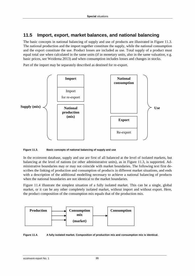
Special situations
ecoinvent-report No. 1 86
11.5 Import, export, market balances, and national balancing
The basic concepts in national balancing of supply and use of products are illustrated in Figure 11.3.
The national production and the import together constitute the supply, while the national consumption
and the export constitute the use. Product losses are included as use. Total supply of a product must
equal total use when calculated in the same units (if in monetary units, also in the same valuation, e.g.
basic prices, see Weidema 2013) and when consumption includes losses and changes in stocks.
Part of the import may be separately described as destined for re-export.
Figure 11.3. Basic concepts of national balancing of supply and use
In the ecoinvent database, supply and use are first of all balanced at the level of isolated markets, but
balancing at the level of nations (or other administrative units), as in Figure 11.3, is supported. Ad-
ministrative boundaries may or may not coincide with market boundaries. The following text first de-
scribes the linking of production and consumption of products in different market situations, and ends
with a description of the additional modelling necessary to achieve a national balancing of products
when the national boundaries are not identical to the market boundaries.
Figure 11.4 illustrate the simplest situation of a fully isolated market. This can be a single, global
market, or it can be any other completely isolated market, without import and without export. Here,
the product composition of the consumption mix equals that of the production mix.
Figure 11.4. A fully isolated market. Composition of production mix and consumption mix is identical.
Supply (mix)
Import
Import
for re-export
National
production
(mix)
National
consumption
Export
Re-export
Use
Production Consumption
mix
(market)
Consumption

Special situations
ecoinvent-report No. 1 87
Figure 11.5 illustrates a partly isolated market where there is no import, but where there is export. In
addition to the market activity for the geographical area, the exports from this market to other markets
are specified as separate transforming activities “…, import from X” with the geographical specifica-
tion of the receiving market and with direct links (specified in ecoSpold field 1520 ActivityLinkId) to
the consumption mix of market X. The local consumption mix still has the same composition as the
local production mix. This situation requires that the local production is flexible, so that an increase in
local consumption does not influence the amount available for export. If this condition is not fulfilled,
the market cannot be regarded as isolated, but is a part of a geographically larger market.
Figure 11.5. A partly isolated local market without imports but with exports. Composition of local production
mix and local consumption mix is identical.
Figure 11.6 illustrates a national (or otherwise administratively delimited) isolated market where the
import is administratively constrained, so that an increase in national consumption does not influence
the import or only affects it in a specific proportion to the national consumption. The contribution of
import is modelled as a separate transformation activity and added as a directly linked input to the
market activity for the national area. If the import is affected in proportion to its share in the national
supply mix, the national consumption mix is equivalent to the national supply mix. Note that the im-
port activity here is an ordinary transforming activity, not a special import activity (ecoSpold field
115 specialActivityType), since the latter does not contribute to the auto-generated national consump-
tion mix.
Local market X:
Rest-of-
World
production
Rest-of-
World con-
sumption mix
(market)
Rest-of-
World
consumption
Local
production
Local con-
sumption
mix, incl. ex-
port
(market)
Local
consumption
Import from
X
Rest-of-World:

Special situations
ecoinvent-report No. 1 88
Figure 11.6. An administratively isolated national market, with constrained import.
In general, administratively isolated markets are becoming less common over time. However, as long
as the national administration decides on the extent and/or technology of imports and/or national ca-
pacity adjustments, it is relevant to regard the market as administratively isolated. Administratively
isolated markets are typically found for products of strategic national interest, such as weapons, food,
and electricity, and where the local administration seeks to protect national producers, such as often
found for the service sectors.
In LCA, the national administrative influence on the electricity markets is of particular interest, be-
cause of the important role of electricity as an input in many product life cycles.
The documentation for a market being isolated, either due to the lack of imports and exports, due to
the lack of imports but with exports from a flexible national production, or due to administrative re-
strictions, is provided in the Geography comment field.
A national balancing of the supply and use of a product, as foreseen in Figure 11.3, can be obtained
by complementing the LCI modelling in Figure 11.6 with the dotted boxes of Figure 11.7:
Export is modelled not only as import in the receiving market, but also as a national production
mix that has the national area as its geographical location (dotted Export boxes in Figure 11.7).
Such export activities have the specialActivityType “export” (ecoSpold field 115) to avoid that
their products are contributing to auto-generated consumption mixes. To give the correct value of
the export, the same activities and data that are included with the market activities are added di-
rectly to the export activity. This includes transport activities, production losses, wholesaler and
retailer activities, and product taxes and subsidies. The inputs of the exported product to the ex-
port activities are added by the database service layer, using the same production volume data
from the activities located in the national area as used when constructing market activity datasets
and production mixes.
National market X:
Rest-of-
World
production
Rest-of-
World con-
sumption
mix, inclusive
export
(market)
Rest-of-
World
consumption
National
production
National con-
sumption
mix, incl. ex-
port
(market)
National
consumption
Import from
X
Rest-of-World:
Constrained
import

Special situations
ecoinvent-report No. 1 89
Figure 11.7. National balancing of supply and use in the situation with a partly and/or administratively isolated national
market (top part of the Figure) and without (bottom part). The products of the dotted activities are not linked to
any further activities in the database, but are included for national balancing only. However, because of their
correct upstream linking, the products can be used as inputs in a specific model without causing any errors.
Rest-of-World:
Export
Use
Nation X:
Rest-of-
World
production
Global con-
sumption mix
(market)
Rest-of-
World
consumption
National
production
National
consumption
Re-export
Rest-of-World:
Supply mix
National market X:
Rest-of-
World
production
Rest-of-
World con-
sumption
mix, inclusive
export
(market)
Rest-of-
World
consumption
National
production
National con-
sumption
mix, incl. ex-
port
(market)
National
consumption
Import from
X
Constrained
import
Export
All import,
incl. for re-
export Re-export
Supply mix
Use
All import,
incl. for re-
export

Special situations
ecoinvent-report No. 1 90
Import is specified with its actual contribution to the national supply mix, disregarding any ad-
ministrative constraints, and is available also in the situation without any national, administrative-
ly constrained market. Import is therefore also modelled as a special import activity (ecoSpold
field 115 specialActivityType) which does not contribute to the auto-generated consumption mix,
but is solely for use in national balancing.
Re-export is added. Re-export activities are modelled as a special re-export activity (ecoSpold
field 115 specialActivityType) to avoid that their products are contributing to auto-generated con-
sumption mixes.
The national supply, combining the output from the special import activity and the output from
the transforming activities within the national boundaries, may be modelled as a supply mix (eco-
Spold field 115 specialActivityType), which does not contribute to the auto-generated consump-
tion mix, but is solely for use in national balancing.
The national use can be calculated as the consumption by activities on the national territory plus
the national export and re-export activities.
Additional advice for data providers:
Datasets for special import activities (ecoSpold field 115 specialActivityType) can only be uploaded to the data-
base when the resulting national balance is correct, which implies that the datasets for national production, con-
sumption, export and re-export must be added to the database before adding the special import activity.
[Changes relative to ecoinvent version 2: The clear distinction between market boundaries and ad-
ministrative boundaries is new. The option for national balancing is new and is related to the (new)
availability of production volume data for all activities. The editor for trade reviews all production
mixes, supply mixes, import activity datasets, and market datasets (consumption mixes) from version
2, to ensure that they are consistent with the new, more precise definitions, and that they fulfil the new
documentation requirements. Changes/additions are either performed or reviewed by the original da-
taset authors, when possible.]

Special situations
ecoinvent-report No. 1 91
11.6 Speciality productions
A speciality production is an activity that has a material for treatment as an input, but which is not a
treatment activity (i.e. it has a positive reference product that determines its production volume). The
production volume of such an activity will be ultimately constrained by the availability of the material
for treatment, and if all the material for treatment available were eventually used by speciality produc-
tions, at least one of these (typically the least competitive) would necessarily be a treatment activity,
since then its speciality product would no longer be the reference product that determines the produc-
tion volume. An example of a speciality production is ethanol from sugar beet molasses, shown in
Figure 11.8.
Figure 11.8. The database-generated model of the treatment of the by-product sugar beet molasses from sugar pro-
duction with the speciality production of ethanol.
Additional advice for data providers:
Materials for treatment should as far as possible not be used as inputs to activities that are not treatment activi-
ties, i.e. speciality productions should only be used when unavoidable. This is due to the effect that speciality
productions have in system models with partitioning. As explained in Chapter 14.4.1, the speciality productions
are allocated in the same way as treatment activities, i.e. in combination with the activity that supplies the materi-
al for treatment. For example, in Figure 11.6, the ethanol will be allocated together with the sugar. If speciality
productions are used too liberally, then large parts of the database may end up as being allocated together.
- molasses,
from sugar beet
- molasses,
from sugar beet
(treatment)
market for
molasses,
from sugar
beet
sugar
molasses, from
sugar beet protein feed,
100% crude
energy feed,
gross
molasses, from
sugar beet, to
generic market
for energy feed
(treatment)
ethanol pro-
duction from
sugar beet
molasses
(speciality
production)
ethanol,
from
fermen-
tation
beet sugar
production

Special situations
ecoinvent-report No. 1 92
11.7 Downstream changes caused by differences in product quality
Since products are defined in terms of their obligatory product properties only, see Chapters 4.4.5 and
9.3, they may differ in terms of non-obligatory properties, and these non-obligatory properties may
influence the later, downstream activities in which the product is used or disposed of, so that these
downstream activities have larger, smaller or different intermediate and/or elementary exchanges.
This is illustrated in Figure 11.9 (left).
In a database context, where products with the same obligatory properties are mixed in the market ac-
tivities, it is not practically possible to separately model the downstream use and disposal activities as
dependent of the specific products used, since this would require these products to be modelled sepa-
rately throughout their entire life cycle, also for those parts of the life cycle where there is no differ-
ence between the products (dotted intersections in Figure 11.9, left). Such a separate modelling would
also not reflect the actual market situation, where the products are not necessarily perceived as differ-
ent by the users. The difference may be something completely irrelevant to the user, such as a contam-
ination that first shows up in the final disposal after several rounds of recycling.
In the ecoinvent database, use and disposal activities are therefore only modelled as average activities
that use consumption mixes as inputs. For a product that has non-obligatory properties that make it
environmentally better or worse in the use and/or disposal stages, these downstream differences to the
average use and/or disposal activities are therefore added specifically and directly as correction da-
tasets to the transforming activity that gives rise to the difference, i.e. that produces the product that
deviates in relevant non-obligatory product properties from the other products on its market (Figure
4.9, right, upper part). In this way, the difference is included in the product system of that particular
product, even when modelling all downstream activities as average activities.
At the same time as a correction dataset is added upstream, it is subtracted from the downstream aver-
age activity by placing it as a direct negative input to the downstream average activity, since the con-
tent of the correction dataset is already included once in the downstream activity (Figure 11.9, right,
lower part). Thus, the same correction dataset is added upstream and subtracted downstream. The up-
stream positive input and the downstream negative input of the correction dataset are scaled to the
production volumes of the two activities that the inputs are provided to. From the perspective of the
average user, these two correction datasets therefore cancel each other out.
A correction dataset has the activity name and reference product “difference to [downstream activity]
caused by [transforming activity that gives rise to the difference], per [unit of reference product (of
upstream or downstream activity)]”. This reference product has neither mass nor any other properties,
since a correction dataset represents a balanced sub-activity of the downstream average activity da-
taset, without a separate reference product.

Special situations
ecoinvent-report No. 1 93
Figure 11.9 (left). The difference in non-obligatory
properties of the products of activities S and N cause
some downstream activities to be different.
Figure 11.9 (right). Downstream activities are modelled
as averages, and the differences are modelled with cor-
rection datasets, moving the differences up to the activ-
ities that cause them. Datasets with dotted lines are
- t
- c
c
.....
m
i
g
Producing
activity S
(Special)
..... Use activity
with product
of activity S
Use activity
with product
of activity N
... Average use
activity with
products of
both S & N
Average
treatment of
both
products
Difference to
average con-
sumption
caused by S
Difference
to average
treatment
caused by S
Difference to
average con-
sumption
caused by S
Producing
activity N
(Normal)
g g
h h
i i
k
m
Generic
final use
activity
t
Difference
to average
treatment
caused by S
Treatment
activity with
product of
activity S
Treatment
activity with
product of
activity N
.....
Producing
activity S
Market for
generic
product g
Market for use of
generic product
(average use
scenario)

Special situations
ecoinvent-report No. 1 94
negative.
Additional advice for data providers:
Correction datasets are most easily produced when all involved datasets (upstream and downstream) are scaled to
their full production volumes, which also makes it most easy to check that the two corresponding correction da-
tasets cancel each other out. The resulting correction dataset may then later be rescaled to any desired unit of ref-
erence product. If the deviating product causes differences in several parallel downstream activities, which is of-
ten the case at least for niche products and infrastructure products, it may be most practical to include the entire
use and/or disposal activity in the correction dataset, so that these activities are completely subtracted from the
downstream averages. Correction datasets can be added to any upstream activity that causes downstream differ-
ences, and is therefore not limited to production activities.
11.8 Outlook: Packaging
Packaging is a complementary product, typically not included in the description and mass of the
packed products. For example, 1 litre of the product “milk, fresh, 3.5% fat by weight” reports the pro-
duction of the milk alone, not its packaging, which is anyway variable. Milk is sold in glass bottles,
plastic bottles and pouches, plastic-lines cartons, etc., each with their specific weights, production and
disposal activities. Therefore, packaging is in general kept separate and added as a complementary in-
put to (and waste output from) the receiving activity where the packed product is used or re-packaged.
Packaging discarded before re-packaging is included as input to the wholesale or retail activity, while
consumer packaging is reported as a separate input to the receiving activity where the packed product
is used.
When the type and weight of consumer packaging is unknown, the default values from Tables 11.1
and 11.2 are applied. These values are the best that are currently available to us, but since their basis
is rather specific (the Danish packaging statistics for 2004) they should only be used as indicative.
More detail, e.g. on the specific types of plastic and paper packaging material, as well as data for sec-
ondary (transport) packaging, can be found in the background documentation on the ecoinvent web-
site.

Special situations
ecoinvent-report No. 1 95
Product group / Packaging Alu Steel Plast Paper Glass
Vegetables and nursery products 0.005 0.005
Fruit, nuts and spices 0.001 0.011 0.003
Meat products 0.001 0.006 0.008 0.002
Processed and preserved fish and fish products 0.001 0.008 0.001 0.004 0.004
Processed and preserved potatoes 0.016 0.017 0.001 0.076
Fruit and vegetable juices 0.003 0.002 0.020 0.001
Processed and preserved fruit and vegetables 0.027 0.014 0.005 0.044
Crude oils and fats 0.001 0.003 0.001
Refined oils and fats 0.005 0.018
Margarine and similar edible fats 0.003 0.013
Dairy products 0.001 0.002 0.005
Prepared pet food 0.005 0.008 0.001 0.002
Preserved pastry goods and cakes 0.002 0.019 0.012 0.007
Cocoa; chocolate and confectionery 0.002 0.001 0.043 0.055 0.002
Noodles, couscous and similar products 0.001 0.021 0.004
Coffee and tea 0.002
0.009 0.007 0.020
Condiments and seasonings 0.001 0.003 0.138 0.013 0.244
Homogenized food preparations and dietetic food
0.018 0.042
Other food products n.e.c. 0.004 0.006 0.009
Distilled alcoholic beverages
0.879
Wines
1.364
Cider and other fruit wines
0.844
Other non-distilled fermented beverages
1.216
Beer 0.001 0.002 0.001
0.008
Mineral waters and soft drinks 0.001 0.021 0.005 0.001
Tobacco products 0.043 0.005 0.027 0.159
Dyes and pigments 0.001 0.013 0.010
Other basic organic chemicals 0.002 0.006 0.001
Pesticides and other agro-chemical products 0.016 0.024 0.029
Paints, varnishes and similar coatings; ink 0.001 0.009 0.016 0.001
Basic pharmaceutical products 0.003 0.012 0.006
Pharmaceutical preparations 0.019 0.214 0.054 0.103
Soap, detergents and polishing preparations 0.001 0.001 0.025 0.015
Perfumes and toilet preparations 0.050 0.012 0.078 0.052 0.045
Glues and gelatines 0.002 0.013 0.026
Essential oils 0.007 0.017 0.007
Photographic chemical material 0.096 0.073 0.192
Other chemical products n.e.c. 0.015 0.030 0.006
Ceramic household and ornamental articles 0.002 0.009
Weapons and ammunition 0.025 0.081
Optical instruments and photographic equipment 0.002
0.042 0.035
Table 11.1. Default values for packaging (kg per kg wet mass of product) for product groups that use different packag-
ing materials. These are average values for these product types. When specific products are packed in only
one of these materials, the amount per kg product should be relatively larger. See also the Table 11.2 on
the following page.

Special situations
ecoinvent-report No. 1 96
Table 11.2. Default values for packaging (kg plastic and paper packaging per kg wet mass of product) for product
groups that use only plastic or paper for packaging.
Product group Plast Paper Product group Plast Paper
Vegetables and nursery products 0.005 0.005 Hollow glass 0.002 0.007
Eggs 0.002 Other processed glass 0.009 0.014
Salt 0.001 Sanitary ceramic fixtures 0.005 0.003
Fresh and preserved meat except poultry 0.006 0.002 Ceramic insulators & fittings 0.001 0.007
Fresh and preserved poultry meat 0.010 0.004 Technical ceramic wares 0.027 0.016
Ice cream and other edible ice 0.037 0.035 Refractory ceramic goods 0.001 0.005
Grain mill products 0.002 0.007 Ceramic tiles and flags 0.004 0.007
Starches and starch products 0.003 0.002 Cement 0.004
Prepared animal feeds for farm animals 0.001 0.002 Precious metals 0.007 0.015
Sugar 0.001 Alu, copper, lead, zinc, tin 0.001
Malt 0.001 0.001 Other non-ferrous metal
products
0.002
Textile yarn and thread 0.013 0.001 Cutlery 0.002 0.002
Textile fabrics 0.012
Tools 0.021 0.041
Made-up textile articles except apparel 0.005 0.002 Locks and hinges 0.001 0.007
Carpets and rugs 0.042
Light containers of metal 0.002 0.005
Nonwovens, except apparel 0.021
Wire products
0.001
Knitted or crocheted fabrics 0.060 0.060 Fasteners, screws, chains
and springs
0.004 0.060
Knitted and crocheted hosiery 0.025 0.281 Other fabricated metal prod. 0.004 0.007
Pullovers, cardigans and similar articles 0.002
Pumps and compressors 0.007 0.007
Leather clothes 0.040
Taps and valves
0.027
Outerwear 0.004
Bearings, gears & similar
0.050
Underwear 0.016 0.008 Furnaces and machinery 0.003 0.005
Furs; articles of fur 0.020 0.013 Electric domestic appliances 0.014 0.021
Luggage, handbags; saddlery & harness 0.003 0.002 Office machinery 0.002 0.052
Footwear 0.013 0.053 Insulated wire and cable
0.023
Wood products 0.009 0.026 Accumulators & batteries 0.016
Paper and paperboard 0.007 Lighting equipment & lamps 0.043 0.050
Household and toilet paper 0.021 0.005 Electr. equipm. for engines 0.214
Paper stationery 0.002 0.022 Other electrical equipment
n.e.c.
0.001 0.006
Wallpaper 0.050 Electronic components 0.014 0.038
Other articles of paper and paperboard 0.002 0.047 Television and radio equipm. 0.007 0.169
Newspapers 0.017 Medical & surgical equipm. 0.045 0.038
Sound recordings 0.014 Measuring equipment 0.011 0.050
Other basic inorganic chemicals 0.001 Parts for motor vehicles 0.010
Fertilizers and nitrogen compounds 0.002 Motorcycles 0.003 0.005
Explosives 0.017 0.037 Bicycles 0.007 0.044
Prepared unrecorded media 0.016 0.007 Chairs and seats 0.011 0.031
Man-made fibres 0.016 Other office & shop furniture 0.007 0.018
New and used rubber tyres and tubes 0.003 Kitchen furniture 0.013 0.037
Other rubber products 0.007 0.029 Other furniture 0.006 0.010
Plastic plates sheets tubes and profiles 0.001 Mattresses 0.016 0.004
Packaging products of plastics 0.002 0.008 Musical instruments 0.006 0.006
Builders' ware of plastics 0.009 0.015 Sports goods 0.011 0.034
Other plastic products 0.003 0.007 Games and toys 0.051 0.046
Flat glass 0.003 0.005 Brooms and brushes 0.018 0.026
Processed flat glass 0.020 0.025 Other manufactured goods
n.e.c.
0.014 0.023

Special situations
ecoinvent-report No. 1 97
11.9 Outlook: Final consumption patterns
When household activities are modelled explicitly as transforming activities, with inputs of raw mate-
rials and outputs of products, final consumption becomes the satisfaction of needs. For example, the
home grown potatoes are combined with purchased food products in the household activity “meal
preparation” that has the product “meal” which combines with the meals from restaurants in a “market
for meal”, which finally may translate into the product “satisfaction of need for food”, which together
with all other need satisfactions combine in a final aggregate consumption/need satisfaction.
The modelling of final consumption/need satisfaction is complicated by the existence of many differ-
ent consumer types, which assign different properties as obligatory for what is accepted as e.g. a
“meal”, so that it is necessary to operate with different markets and market niches for meals, which
together with other specific preferences of the consumer types combine into final consumption or
need satisfaction patterns per consumer type.
There are several suggestions on how to classify human needs. We apply the modification suggested
by Weidema et al. (2005) to the Segal (1998) set of core economic needs, which has the advantage
over other classifications that its applicability has been demonstrated in practical empirical work and
that it provides a stronger linkage between consumption and affluence and its basis in products. The
11 need-based consumption groups are:
Housing
Food
Leisure
Social care
Education
Health care
Security (including insurance)
Communication
Clothing
Hygiene
Other consumption not elsewhere classified (mainly “economic infrastructure” expenditures, such
as interest etc. on financial investments, and economic affairs and services).
In national statistics, final consumption is typically recorded as the products directly or indirectly pur-
chased by households. When recorded in this way, the household activities, e.g. the relation between
shopping, car driving, fuel use and its emissions, are not included in the final consumption. However,
at a more detailed level, statistics are available on the consumption patterns of different household
types, depending on parameters such as household size, income level, dwelling type, etc. These data
are interesting for understanding the driving forces behind consumption and for modelling changes in
the household parameters. To take advantage of these data sources, the final consumption patterns
from the statistics are translated into demands for the corresponding household activities per house-
hold type, thus integrating the household consumption patterns with those of the consumer types into
one overall model of final consumption or need satisfaction.
Special situations
ecoinvent-report No. 1 98
11.10 Linking across time
11.10.1 Lifetime information / Stock additions
In life cycle inventory modelling, long-lived products are typically represented by steady-state mod-
els, e.g. a car will typically be modelled with the current production technology, the average life time
emissions and the current waste treatment technology, all divided by the lifetime of the car. Effective-
ly, this means that - in this LCI modelling - the net additions to stock of these long-lived products are
simply contributing as physical inputs to the waste treatment activities of the current year.
When lifetime information is available for a product and/or waste, and waste treatment datasets are
available for the period that the product becomes waste, the waste treatment and the accompanying
emissions can be placed at their correct point in time.
It is strived for to make lifetime information available for long-lived products and to make waste
treatment datasets available for future periods, so that current net additions to stock of these products
can be modelled as becoming waste at the correct period, and thus use the waste market that corre-
sponds to this period.
Outlook: It is possible to automatically identify by-products and wastes with a property “lifetime” in
excess of one year7 as an addition to stock (ecoSpold field OutputGroup option 5 = StockAdditions),
thus distinguishing this “future waste” from the waste outputs of the current year. For such stock addi-
tions, the database service layer would then be able to identify the years in which the stock will be-
come waste (using the lifetime and any uncertainty information provided on this) and link this waste
directly to the corresponding future waste treatment markets. If a treatment market is missing for a
specific year, the corresponding treatment market for the nearest preceding time period would be ap-
plied.
In LCI modelling, it is the consumption activities that demand the necessary upstream production ac-
tivities. Therefore, a similar automatic linking of the future consumption activities of long-lived prod-
ucts cannot be made, since this would require that the consumption activities were inputs to the infra-
structure activities in the same way as the waste treatments are. Thus, such dynamic modelling of the
consumption activities of long-lived products still requires additional, manual linking by the database
user of the relevant accumulated systems datasets across time.
However, inputs to an infrastructure dataset (a dataset with a reference product having the property
“capacity” or “lifetime_capacity”) may have a specific, direct link (using the activityLinkId) to a fu-
ture activity. This may be relevant for maintenance activities or components of infrastructure that
have a shorter lifetime than the composite infrastructure, e.g. windows in a building, or tyres on a car.
When linking to datasets of future years, only accumulated systems datasets would be linked to, to
avoid an endless calculation task, since practically all datasets within a time period are linked to each
other, and linking to just one dataset from a future year therefore would involve the entire economy in
that future year, with the additional possibility that datasets of this year also link to even more future
years.
Applying the output category “stock additions” will remove the requirement of direct equivalence be-
tween capital investments and waste in any given time period. When using the ecoinvent database in
connection to data from national accounting (see Weidema 2013), this will allow to balance the com-
7 This is relevant for by-products/wastes only, because reference products with a lifetime in excess of 1 year are always ser-
vices, see Chapter 4.11, i.e. the stock addition/future waste occurs always directly as an output of the activity that produces
the long-lived product.

Special situations
ecoinvent-report No. 1 99
plete economy for a given year, based on the actual investments in capital goods, and the actual waste
amounts of that year, without any artificial requirement that these should match.
[Changes relative to ecoinvent version 2: In version 2, each dataset is only available for one time
period, and all datasets are linked without regard to their indicated time period. In version 3, only da-
tasets for the same time period are linked, except for the described situation of stock additions, which
makes use of the new option to add lifetime as a numerical property to intermediate outputs, and if
links across time are made using the activityLinkId.]
11.10.2 Long-term emissions
Emissions that occur over large time frames of substantially more than 100 years are assigned to spe-
cific subcategories (labelled "long-term"). Such long-term emissions occur in landfill sites (leaching),
in uranium mining and milling sites (radon emissions) and – probably – final repositories of nuclear
waste. For landfill emissions and uranium mining and milling sites timeframes of 60'000 and 80'000
years, respectively, are chosen. These activities release pollutants to “air, low population density”, to
“water, river” and to “water, ground-“ during very long time scales. The ecoinvent database contains
corresponding long-term subcategories in order to distinguish these long-term emissions from the
ones occurring within the first 100 years.
[The issue of how best to include long-term emissions is currently under consideration in a separate
ecoinvent research project]

Special situations
ecoinvent-report No. 1 100
11.11 Using properties of reference products as variables
[Feature considered for implementation later: While the performance of the database service layer
as described in this section has been implemented, additional experimentation and testing was found
to be required before taking this feature into general use. It has therefore not been used in practice for
any datasets in the version 3.0 release. Even without the software implementation, the specification in
this chapter can be used for manual implementation.]
When one or more exchanges of an activity dataset are expressed as mathematical relations involving
a property of the reference product, and this property is not a fixed property (see Chapter 5.6.7), the
value of the property may change depending on the setting of the property in the dataset that has the
reference product as an input. Each setting of the property value effectively represents a different
product. This can be seen as a special case of combined production (see Chapter 5.3) in which each
such property represents a combined product, with the important difference that the properties are not
traded separately from the product that carries the properties. Like for other cases of combined pro-
duction, a sub-division of the multi-product dataset is required, so that the specific dependencies of
each variable property are expressed in separate datasets. For example:
If a dataset for impact extrusion of aluminium, with the reference product “impact extrusion of
aluminium, cold”, has one or more of its exchanges defined as a mathematical relation to the
property “number of deformation strokes” (variable name: “strokes”) of the reference product,
two datasets are required: One with the reference product “strokes of impact extrusion of alumin-
ium, cold” and one with the reference product “impact extrusion of aluminium, cold, property in-
dependent”, in which the first dataset contains all the mathematical relations that involve the
property “strokes” and the second contains all the other exchange data that are not dependent on
this (or any other) property of the reference product.
If a dataset for waste incineration, with the negative reference product “waste”, has one or more
of its exchanges defined as a mathematical relation to the property “cadmium content” of the
waste, two datasets are required: One with the negative reference product “cadmium content of
waste” and one with the negative reference product “waste, property independent”, in which the
first dataset contains all the mathematical relations that involve the property “cadmium content”
and the second contains all the other exchange data that are not dependent on this (or any other)
property of the reference product.
For each new variable property of the reference product (i.e. a property included in a mathematical
relation of another exchange), a new dataset is required (if there is at least one other activity dataset
that has the reference product as an input with a different amount of the variable property). Each addi-
tive element (summand) of the mathematical relation can only contain one property of the reference
product. Composite or nested properties can be used for situations where multiple relations exist (e.g.
when an emission is dependent on both the degradability and the elemental composition of a waste).
Figure 11.10 illustrates the original and the derived datasets and how these are linked to the activities
that require the reference products. The variable property is added as a by-product with the name
“[property name] of [name of reference product]” and the mathematical relation is changed to refer to
the amount of this new by-product, while the original property is deleted from the reference product,
which is renamed to “[name of reference product], property-independent”. All exchanges that were
originally expressed as fixed amounts are re-formulated as mathematical expressions relating to the
reference product, i.e. the fixed amount “40” translates to “40/A”, where A refers to the amount field
of the reference product. The market activity dataset for the reference products is likewise sub-
divided, with all other exchanges and properties remaining with the property-independent reference
product, so that the new property-specific market activities have no additional exchanges besides the
reference product.

Special situations
ecoinvent-report No. 1 101
Figure 11.10. The original and derived datasets where a property Y of the reference product is used as a variable, and
the original dataset requiring this reference product, but with a different value for Y, where the input is also
subdivided. Note that the mass balance (and other balances) may be kept intact for the subdivided activi-
ties, (as illustrated by the change in dry mass of the reference product) when such adjustments are made
during a manual sub-division, but since properties do not themselves have properties such as mass, such
adjustments are not made when the sub-division is made automatically by the database service layer (see
Chapter 14.1, linking rule no. 4). However, the aggregated systems results are not affected by this.
Other datasets supplying the same reference product to the same market are subdivided in the same
way. If such datasets do not have the same property of the reference product as a variable property,
the exchanges of this dataset are interpreted as independent of this property, and their fixed amounts
thus simply re-formulated as mathematical expressions relating to the re-named reference product.
When the subdivision is performed by the database service layer, the subdivided datasets keep the
same activity ID as the original dataset, which implies that the product name is required to distinguish
the datasets from each other.
product A product A 2 kg product A;
property Y = 3g/kg
1 kg reference product A; dry mass = 1 kg; property Y = 5g/kg
Original datasets:
Activity
producing A Exchange B; amount = f(A, property Y) = 0.25 + 0.8*Y g
Exchange C; amount fixed (40g per kg A)
Activity
requiring
product A
Derived datasets and links to supply 2 kg of A:
6 g property Y of
reference product A Activity
producing
property Y
of A
Activity
producing
A, property
independent
Exchange C; amount = f(A) = 2 kg *40 g/kg = 80 g
Exchange B; amount = f(Y) =
0.8*Y g = 0.8*2kg*3g/kg = 4.8 g Activity
requiring
product A 2 kg reference product A,
property independent; dry
mass = 1.994 kg
Exchange B; amount = f(A)
= 2*0.25 g = 0.5 g
Market for
product A
Market for
product A
Market for
property Y
of product A
(new)

Special situations
ecoinvent-report No. 1 102
11.12 Market averages of properties
When a property of an output of an activity is not fixed (re. fixed properties, see Chapter 5.6.7), dif-
ferent transforming activities may supply the same product with different values for the same proper-
ty. For example, different suppliers of lignite, even to the same market, may provide lignite with dif-
ferent sulfur contents.
This situation is more general than the specific situation described in Chapter 5.8.
As part of the linking of the different activities into product systems, see Chapter 4.14 and Chapter 14,
the database service layer calculates the inputs to each market activity from different suppliers in pro-
portion to their available production volumes, and calculates the resulting production volume of the
market output. In addition, those product properties that are common to all the suppliers to the market
are added as properties of the market reference product, and the values of these properties are calcu-
lated in proportion to the supplied production volumes (this calculation does not apply to the property
“price”, since market prices are not simple averages of production prices).
These properties of the market outputs can be applied in further calculations. For example, the sulfur
content of lignite may be used to determine the emission of sulfur dioxide in the activities that use the
lignite as a fuel. To avoid circular references in the database, the calculated properties of the market
outputs are not automatically transferred to the activities that use the market outputs, but remain
available in the market datasets for information purposes and possible manual adjustments of the
properties in these receiving activities. This transfer of information is of course only relevant when
there are different values of a property among the suppliers to the same market and the receiving ac-
tivity uses the property values for calculations.
11.13 Use of transfer coefficients
Transfer coefficients is a feature of the new ecoSpold 2 format, but it has not yet been decided wheth-
er and when ecoinvent will support datasets with transfer coefficients.

Validation and review
ecoinvent-report No. 1 103
12 Validation and review
Validation is the automatic software routine to check that data are valid according to the internal rules
set for the ecoinvent database.
Review is the manual inspection of the data and commenting on any discovered errors or anomalous
data that require additional explanation or justification.
12.1 Validation
The automatic validation of ecoinvent data covers the
accordance with the ecoSpold 2 data format,
accordance with additional ecoinvent-specific rules, as described in this document,
plausibility of the data,
and takes place in several steps:
The ecoEditor software, used by data providers to create and edit data for the ecoinvent database, se-
cures the validity of the data against the ecoSpold 2 data format already during editing. Likewise,
some validations of accordance with ecoinvent-specific rules can also be performed directly upon data
entry, e.g. “Time period shall be minimum one year”.
Other validation checks can be made off-line (i.e. without contact to the ecoinvent database) in the
ecoEditor software, upon user request, typically before storing an edited dataset, e.g. “An ISIC class
must be chosen”, and “More than one reference product in the same activity dataset”. The latter is an
example of a validation check that does not lead to a rejection of the dataset (i.e. it can still be submit-
ted to the database for review), but results in a warning to the user (here that “'It is unusual to have
more than one reference product. This occurs only when no alternative production routes exist for
these products. If you are in doubt which of the products is the reference product or if you think there
should indeed be more than one reference product for this activity, please consult the ecoinvent Data
Quality Guideline Chapter 11.1 for further advice.”).
Other validation checks require contact to the production version of the ecoinvent database, because
they require a check against data that already exist in the database, e.g., “Global dataset must exist be-
fore non-global datasets can be uploaded”, and “Production volume of datasets for a specific activity,
time period and macro-economic scenario must not exceed production volume of the corresponding
global dataset”. Such validation checks also apply for deletion of datasets, e.g. “A parent dataset can-
not be deleted” (deletion of datasets can only be done by the ecoinvent editors, see Chapter 12.2, but
can be suggested on the relevant discussion boards on the Editor's pages, see Chapter 16.4.)
Validation checks that require contact to the database can either be performed via the ecoEditor soft-
ware when this is in on-line contact with the database, [Feature considered for implementation lat-
er: or by submitting the dataset to the ecoinvent database for validation via a web-browser]. When us-
ing the ecoEditor on-line, the validation result will be inserted directly in the dataset (in the ecoSpold
field 3340 Validation details). Only the latest validation result will be stored (i.e. any previous valida-
tion results will be over-written). If submitting a dataset via a web-browser, the validation result (a
text message) will be returned by e-mail.
The plausibility checks generally do not lead to rejection of a dataset (i.e. it can still be submitted to
the database for review), but results in a requirement to justify the anomalous value in the adjoining
comment field, if the anomalous value is maintained. An implausible entry without an adequate justi-
fication will be returned by the reviewer.

Validation and review
ecoinvent-report No. 1 104
Plausibility checks generally compare the data entries to similar entries in similar datasets. Thereby,
the completeness of the data is checked (missing exchanges or missing entries in fields where all simi-
lar datasets have entries); it is checked that the entries fall within expected ranges (relative to the
amount of the reference product or relative to well-established relations between different amounts
and/or properties of specified exchanges). Results of mass and monetary balances are also reported in
the validation results.
The plausibility checks obviously relate to the existing database, specific clusters of similar datasets
within the database, and knowledge about what are typical and important errors and relationships be-
tween individual data values within each cluster. This knowledge is built up over time, and is based
on a continuous learning cycle of learning from past errors, software-supported explorative data anal-
ysis, interaction with expert knowledge, and cluster analysis. Thus, the plausibility checks will im-
prove over time, and will be implemented in the ecoEditor and the database software, as part of the
continuous maintenance and updating. [At the time of the release of version 3.0: Plausibility checks
are largely missing]
[Changes relative to ecoinvent version 2: Validation is more extensive.]
12.2 Review of dataset and documentation
All transforming activity datasets are reviewed by at least three experts prior to the storage of the da-
tasets in the database. [At the time of the release of version 3.0: Not all datasets have so far been re-
viewed by at least three experts. Such datasets are to be submitted to a more extensive review at a lat-
er date.]
12.2.1 Types of editors
There are three overall types of ecoinvent editors: activity editors, cross-cutting editors, and LCIA ed-
itors. Cross-cutting editors can further be sub-divided in geographical editors, inventory indicator edi-
tors, meta-data editors and language editors. Each of these types of editors will be described in the
following:
Activity editors: Activity editors are responsible for reviewing of data for a specific industry, technol-
ogy or other human activity. The activity editor is the main reviewer for a dataset; she/he is the first to
receive a submitted dataset, and the last to accept it for final upload to the current beta-version of the
database. Activity editors are typically leading (LCA) experts within their activity area. The activity
editors divide the work between them according to the ISIC (Rev. 4, ecoinvent-amended) codes of the
datasets and/or the type of dataset. The main editor may re-assign a dataset to a co-editor with special
expertise but still request to remain as main editor for the dataset. In this case, the dataset will first be
reviewed by the co-editor and then by the main editor for overall consistency. An activity editor is in
principle responsible for all datasets within an activity area, disregarding any geographical differences
(exactly to ensure global consistency of activity datasets, i.e. across all geographies). When a dataset
has been reviewed by the activity editor, it is passed on to the cross-cutting editors:
Geographical editors: A geographical editor is responsible for datasets that fall geographically within
a specific country or other geographical area, ensuring that geographical variation in technologies are
correctly and consistently captured and integrated across all datasets for that area. If the ecoinvent
Centre cooperates with a national data collection initiative in a country, the geographical editor for
that country will typically be appointed after suggestion by the national data collection initiative.

Validation and review
ecoinvent-report No. 1 105
Inventory indicator editors: An inventory indicator editor is responsible for a specific emission (or
group of emissions), e.g. particle emissions, or other environmental pressure indicators (e.g. re-
sources, land use, noise, social aspects)8, ensuring the consistency across all datasets.
Meta-data editors: A meta-data editor is responsible for ensuring the consistent use across all datasets
of a specific database field (or group of fields) or master file entries, e.g. for name fields, statistical
classifications, free documentation fields, supply-use data, geography fields, system models, scenari-
os, uncertainty fields, and product properties. Meta-data editors for required product properties, such
as mass, carbon content and price, have the additional task to suggest data when these are not supplied
by the data provider.
Language editors: A language editor is responsible for checking consistency and quality of transla-
tions within a specific language version of the ecoinvent datasets, and may maintain a vocabulary for
automatic pre-translations. Language editors will only receive datasets for review when they contain
translated fields in their specific language.
LCIA editors: LCIA editors are responsible for impact assessment datasets, not activity datasets. In
this way, they work in parallel to the activity editors. There are two kinds of LCIA editors: LCIA
method editors and LCIA pathway editors. An LCIA method editor is responsible for the maintenance
of the ecoinvent version of a specific LCIA method (CML, Ecoindicator, etc.). The LCIA method edi-
tors are both responsible for the correctness of the mapping of the environmental pressure indicators
(“Elementary exchanges”) between the ecoinvent inventories and the specific LCIA method, and for
the correspondence of the numerical entries in the ecoinvent implementation with those of the original
published method. An LCIA pathway editor is responsible for the consistency of the implementation
of a specific impact category and/or pathway (for noise, water resources, etc.) across all relevant
LCIA methods. LCIA editors are involved both when an LCIA method is updated by the method de-
veloper, and when new environmental pressure indicators are added to the ecoinvent database. The
only cross-cutting editors which are relevant for impact assessment datasets are the language editors.
Thus, when an impact assessment dataset has been reviewed by the LCIA editor(s), and it contains
translated fields, it is passed on to the language editor.
12.2.2 The flow of a dataset through the editorial process
When a data provider submits the dataset via the ecoEditor software [Feature considered for im-
plementation later: or via the ecoinvent web-site], the software stores it and assigns it to the relevant
editor. For a transforming activity dataset this will be determined by the statistical classification as-
signed to the dataset by the data provider. For production and supply mixes and market activity da-
tasets this is the editor for wholesale and retail trade. For import datasets and supply-use data, this is
the meta-editor for supply-use data. For an LCIA method dataset this will be determined by the name
of the method or impact category.
The original data provider (author) of a dataset can ask to be ‘active author’ and will then be informed
whenever there are other data providers that suggest modifying the dataset in question and can decide
to take over the suggestion (and thus remain as author of the dataset) or comment on the suggested
modifications before the dataset is passed on to the activity or LCIA editor.
If the dataset is an edited version of an existing parent dataset, the consequences for the child datasets
are reviewed at the same time as the edited parent dataset.
The main editor may pass on the dataset and review responsibility to a co-editor if temporarily una-
vailable due to workload, holidays or illness, or if judging that the co-editor has more scientific exper-
8 Environmental pressure indicators are called ”Elementary Flows” in the ISO 14040 series, and “elementary exchanges” or
“exchanges with the environment” in ecoinvent.

Validation and review
ecoinvent-report No. 1 106
tise for the particular dataset in question. When passing on a dataset to a co-editor, the original re-
sponsible editor indicates whether the co-editor thereby becomes the responsible editor for this da-
taset or whether the original main editor remains as responsible editor, in which case the dataset will
first be reviewed by the co-editor and then by the main editor for overall consistency. In case of con-
flicts of interests, any editor is required to pass on the dataset and review responsibility to a co-editor,
and shall not demand to remain as responsible editor.
Having accepted the dataset for review, the responsible editor adds any review comments to the file. If
a dataset is a delta/child dataset or a new version of an existing dataset, only those parts of the dataset
are reviewed that are different from the parent or are affected by the changes. The purpose of the re-
view is to check the dataset against the data quality guidelines in this document, to check that the re-
sult of the automatic validation has been adequately addressed, and to check the plausibility of the da-
taset against the “real life” activity that it is intended to represent. As part of the review, the editor
may also compare the new dataset with an older version or a similar dataset. For delta/child datasets,
the editor also considers whether entries correctly belong in the delta dataset, or should rather have
been placed in the parent dataset.
If the review comments are of a nature that revision by the data provider is required, the commented
dataset is returned to the data provider for re-submission. This procedure may continue until the re-
sponsible editor is satisfied with the quality of the submitted dataset.
When the responsible editor has accepted the dataset, the data provider is informed and the dataset
now passes on to the cross-cutting editors. Depending on its content, the dataset can be passed on in
parallel to several cross-cutting editors:
All activity datasets except global datasets are passed on to the relevant geographical editor.
Inventory indicator editors receive activity datasets if they contain data on their specifically monitored
environmental pressure indicators (elementary exchanges). If the dataset is a new version of an exist-
ing dataset, it is only passed on if there are changes for the monitored indicators. More than one in-
ventory indicator editor may be involved in the review of the same activity dataset.
Meta-data editors receive activity datasets if they contain information in one of the fields specifically
monitored by them. If the dataset is a new version of an existing dataset, it is only passed on if there
are changes for the monitored fields. More than one meta-data editor may be involved in the review of
the same activity dataset.
Language editors receive datasets if they contain translated fields in their specific language. Datasets
that have multiple languages may thus be passed on to several language editors in parallel. If the da-
taset is a new version of an existing dataset, it is only passed on if there are changes for the text or
name fields, or when a new language has been added.
If responses are given by one or more cross-cutting editor, these responses are automatically accumu-
lated into one review version, which is passed on to the data provider for corrections and resubmis-
sion. The resubmitted dataset is returned to the editors which have given comments. This procedure
may continue until the cross-cutting editors are satisfied with the quality of the submitted dataset.
When the dataset has successfully passed the cross-cutting review, the data provider is informed and
the dataset passes back to the responsible editor. If there has been changes made during the cross-
cutting review, the responsible editor performs a final review. After this final review, the responsible
editor uploads the dataset to the current production version of the database, and the data provider is
informed.
Editors seek to process submitted datasets within 14 days of receipt, but may request a prolongation
of the review period during peak load, in which case the data provider will be informed. The mini-
mum time between submission of a dataset and its inclusion in the production database is one month,
but will usually require more time due to several rounds of comments and replies between editors and
data providers.

Validation and review
ecoinvent-report No. 1 107
The review procedure is comparable to the critical panel review specified in the ISO standards.
It has to be emphasised that the responsibility for the contents of all datasets remains with the person
and institute who supplies the data. The reviewer helps to improve the quality of datasets with his or
her suggestions. But it is the final decision of the dataset author whether all proposals for corrections
of the data are implemented, just as it is the decision of the activity editor whether a dataset can be in-
cluded in the database or not. If an editor repeatedly returns a dataset, and this is regarded by the au-
thor as unfounded, the author may address a complaint to the ecoinvent LCI Expert Group that has the
final decision authority on scientific matters raised by the Editorial Board or arising from complaints.
[Changes relative to ecoinvent version 2: Review is more extensive and now performed by domain
experts.]
12.3 “Fast track” review for smaller changes
Outlook: For adding tags to a dataset and for smaller corrections to a dataset (e.g. correcting spelling
errors, adding, editing or deleting single entries that are obviously wrong), which do not require a full
review of the entire dataset, a “fast track” submission procedure via the ecoinvent web-site
<www.ecoinvent.org> is considered. This will avoid the need to download and install the ecoEditor
software if it is only single entries that are to be submitted for review. The review procedure for such
submissions will also be streamlined, to limit the workload on the editors, and to reduce the time be-
tween submission and publication.
12.4 Confidentiality
Confidentiality concerns of a data provider and requests for confidentiality agreements should nor-
mally be referred to the ecoinvent database administrator. When the data provider has set the ac-
cessRestrictedTo to either “2 = ResultsOnly” or “3 = Restricted”, the dataset will not even arrive at
the editor’s desk, but will be redirected to and handled by the ecoinvent administrator directly. Confi-
dential datasets are subject to the same data quality guidelines as any other ecoinvent dataset, but the
review procedure will be performed under the direct management of the ecoinvent administrator that
signs and/or manages the necessary confidentiality agreements, also in case of re-delegation of the re-
view to independent reviewers.
The ecoinvent Centre accepts no responsibility for confidentiality agreements made directly between
editors and a data provider.
12.5 On-site auditing
Branded datasets require on-site review by an ecoinvent-approved auditor. A visit to the factory and
auditing of the books is required to determine that the activity is correctly and completely represented
in the dataset. Audits are performed according to ISO 19011 and with Weidema et al. (2003) as tech-
nical basis. On-site audits may require the signing of a confidentiality agreement, and is always organ-
ised with the assistance of the ecoinvent administration.

Embedding new datasets into the database
ecoinvent-report No. 1 108
13 Embedding new datasets into the database
Outlook: The ecoinvent data are intended to cover all aspects of the societal economy, although in
varying degree of detail. For industries where not all products are already specifically included in the
database, at least one activity dataset should represent the production of unspecified products of that
industry. For example, while the ecoinvent database contains a large number of individual pesticides,
there is also an activity representing “pesticide production, unspecified” with the reference product
“pesticide, unspecified”.
The implementation of this completeness would imply that any new dataset, which is not a delta da-
taset for a child to an existing dataset, would always be a disaggregation of an existing dataset. For
example, adding a new pesticide production would be a disaggregation of the activity “pesticide pro-
duction, unspecified”. The production volume of the “pesticide production, unspecified” would be re-
duced by the production volume and exchanges of the new, specified pesticide.
The disaggregation would also ensure that the ecoinvent database would remain complete and non-
redundant, i.e. for any given activity there is only one dataset that is the relevant dataset.
For a data provider of a new dataset, this would imply that at least two datasets are to be supplied at
the same time: The new, specific dataset and the residual of the original, more unspecific dataset.
These two new datasets together sum up to the original dataset. If the original dataset is not believed
to represent the correct sum of the disaggregated datasets, a corrected version of the original dataset
has to be submitted before or together with the disaggregated datasets.
It is considered to support disaggregation in a future version of the ecoEditor software. Until then, the
disaggregation and the check against the original dataset have to be performed manually.
A disaggregation of an activity also implies a disaggregation of its reference product. For example,
the disaggregation of “knitted nets” into “knitted textile bags” and “fishing nets”. Since the reference
product of the original activity is an input to other activities in the economy, the datasets for these ac-
tivities will also have to be adjusted, so that they instead of having inputs of the original reference
product now have inputs of one or more of the disaggregated reference products. By default, the
ecoinvent database would assume that all activities that had inputs of the original reference product
will have inputs of all the disaggregated products in proportion to their new production volumes. This
implies that the receiving activities are unchanged, except for the higher resolution in the intermediate
input, and will provide the same results for their accumulated systems. However, this does not take
advantage of the additional information provided by the new disaggregated activities. The food indus-
try will still receive a part of their textile bags in the form of fishing nets, and the fishing industry will
still receive too many textile bags. The authors and/or editors of the affected datasets should therefore
be informed about the availability of this additional resolution, and asked to confirm the default dis-
tribution of the new disaggregated inputs, or to provide another distribution, thus allowing e.g. the
food and the fishing industry to remove the unwanted inputs and place them on the correct disaggre-
gated activity that now has become available. Such consequent changes, resulting from the availabil-
ity of new resolution in an input, would pass through the “fast track” review procedure, see Chapter
12.3.
The ecoinvent LCI Expert Group may decide that some datasets representing unspecified products
may be of such low quality that they are not to be included as inputs to other activities, but should on-
ly be available in the ecoinvent database for information purposes. Such datasets are provided with a
tag “low-quality unspecific dataset”. In the activities that require such inputs, the missing inputs are
mentioned as excluded inputs in the field ‘IncludedActivitiesEnd’ and the input may be quantified by
an elementary exchange “missing input from technosphere” with reference to the amount and unit of
the excluded unspecified products. Further detail on the missing input may be described in the com-
ment field of this exchange. This facilitates the inclusion of such inputs when data of better quality

Embedding new datasets into the database
ecoinvent-report No. 1 109
becomes available, allows the inclusion of the excluded inputs in mass and monetary balances, allows
an estimation of the excluded part of any product system, and allows the database users to add the
missing inputs manually.

System models and computation of accumulated system datasets
ecoinvent-report No. 1 110
14 System models and computation of
accumulated system datasets
The ecoinvent database is not just an LCI data library but also an LCI data network. The unlinked da-
tasets of the ecoinvent unit processes are interlinked by the database service layer. All intermediate
goods and service inputs to a unit process, be it the consumption of electricity, the demand for work-
ing materials, the use of the road infrastructure, are linked to other unit processes that supply these in-
termediate goods and services. This means that any change in one unit process influences the accumu-
lated LCI results for almost all other unit processes. Depending on the magnitude of the change, this
influence may be negligible for the majority of the datasets, but it may also be significant to many or a
few datasets.
The ecoinvent database stores the unit process datasets as unlinked, multi-product datasets, i.e. with
inputs specified solely in terms of product names, without requiring specification of the supplying ac-
tivities, and typically with more than one product output. This is the way the datasets are obtained and
entered by the data providers and this is how the unit processes are normally presented to the end us-
er.
For the purpose of calculating the accumulated system datasets, the database creates linked, single-
product datasets from the unlinked, multi-product datasets, with the help of database-wide modelling
rules. An unlinked, multi-product dataset and its derived linked, single-product datasets have the same
universally unique identifier (UUID) and name, and are distinguished by the field “systemMod-
elName” (and for subdivided datasets by the reference product).
Two classes of system models are distinguished: System models with partitioning (allocation) and
system models with substitution (system expansion).
14.1 Rules common to both classes of system models
It is a prerequisite for linking of any dataset that a specific geography, time and macro-economic sce-
nario is declared in the relevant fields. Linking only takes place within this specific context (linking to
same or larger geography and time, and same macro-economic scenario).
Some linking rules are identical for both classes of system models:
1) By-products/wastes that are identified by the database service layer as materials for treatment (see
Chapter 4.8) are always moved to be negative inputs of the same activities, in order to include the
treatment activities for the materials into the product systems. Since a negative input is the same
as a positive output, this operation does not affect the mass, energy and monetary balances of the
activities.
2) An intermediate input to an activity, which does not already have an activityLinkId, is always
linked directly to the local market activity dataset that supplies this input as its reference product.
The database service layer identifies the local market activity dataset based on the geographical
location of the activity, matching this location with the available market that is equal to or covers
this location. Since markets do not overlap, there will generally only be one such market activity
for each intermediate input. If the activity is defined for a geography or time that spans over more
than one market, each of the market activities contribute in proportion to their production volume
(calculated as described in Chapter 14.2), implying that the database service layer will duplicate
the intermediate input to match the number of supplying markets and subdivide the amount of the
intermediate input over these in proportion to the production volume of each market. For activi-
ties with the geographical location "Rest-Of-World" (ROW) the inputs are linked to those suppli-
ers that are not used as suppliers by any of the corresponding geographically specified (non-

System models and computation of accumulated system datasets
ecoinvent-report No. 1 111
ROW) activities, and if all these suppliers are used, to the supplying activity with the largest pro-
duction volume.
3) For situations of variable properties of the reference product, the reference product is subdivided
by the procedure described in Chapter 11.11,
4) For situations of combined products, the dataset is subdivided into an equivalent number of da-
tasets, by the procedure described in Chapter 5.3. This procedure applies both to the datasets of
combined production and the datasets generated from the variable properties, as described in the
previous point.
The modifications described by these four rules are performed by the database service layer in the de-
scribed order, before any other modification or calculation of the datasets for linking to suppliers and
partitioning or substitution, except for the calculation of market production volumes required by rule
2.
14.2 System models with linking to average current suppliers
In many system models, the inputs to each market activity are modelled as coming from all those
transforming activities within the geographical area of the market activity, which have the market ref-
erence product as an output, in proportion to their available production volume.
In current practice, this linking to average current suppliers is applied in all system models with parti-
tioning, although there is no formal connection between partitioning and any specific linking rule for
suppliers.
The ecoinvent database service layer automatically:
Identifies these transforming activities, based on geographical matching,
Adds an input to the market activity from each of these transforming activities,
Adds the corresponding unique IDs of the transforming activities to the ActivityLinkId (ecoSpold
field 1520) of the market inputs, thereby directly linking the inputs to the transforming activities,
Calculates the amount of input from each transforming activity in proportion to its production
volume, as indicated in the ecoSpold field 1530 productionVolumeAmount of each transforming
activity, subtracting any production volume that is required by transforming activities via direct
links (ActivityLinkId; ecoSpold field 1520) and therefore not supplied via the market,
Sums up the production volumes, and adds the sum as the production volume of the output of the
market activity,
Calculates the production-volume-weighted averages of any properties that are common to all the
transforming activities (with the exception of the price property) and places these averages as
properties of the output of the market activity,
[Feature considered for implementation later: Propagates the price information throughout the
linked datasets by: Copying the price property of market reference products to all intermediate in-
puts that are supplied from markets, calculating the price property of the corresponding inputs to
the markets as ((price*amount of the market reference product - price*amount of any other inter-
mediate or elementary input with a price property)/amount of the reference product), copying the
resulting price property of the market inputs to all intermediate outputs that are supplied to the
market, and finally adding the price property to intermediate inputs that are supplied directly from
transforming activities by copying it from the corresponding intermediate outputs.]
In combination with the rule for linking transforming activities to their local markets (rule 2 in Chap-
ter 14.1), the above rules for linking market activities results in a database that is fully linked up-
stream, i.e. all inputs to all datasets are directly linked to their specific supplying activities.

System models and computation of accumulated system datasets
ecoinvent-report No. 1 112
14.3 System models with linking to unconstrained suppliers
In some system models, production constraints are taken into account, so that only unconstrained sup-
pliers are included. Besides this, the inputs to each market activity are modelled much in the same
way as in models linking to average current suppliers.
The unconstrained suppliers to the market are identified by the database service layer as those trans-
forming activities, within the geographical area of the market activity, for which the market reference
product is a reference output (i.e. not a by-product, since the volume of a by-product is per definition
constrained by the corresponding reference products), and which has a technology level (see Chapter
5.5) that corresponds to the specific rule for the particular system model, see Chapter 14.6.
For each of the identified unconstrained suppliers, the ecoinvent database service layer then:
Adds an input to the market activity, with the corresponding unique IDs of the supplier as Activ-
ityLinkId, thereby directly linking the input to the specific supplier,
Calculates the amount of input to the market activity in proportion to the production volume of the
supplier, subtracting any production volume that is required by transforming activities via direct
links and therefore not supplied via the market,
Calculates the production-volume-weighted averages of any properties that are common to all the
suppliers and places these averages as properties of the output of the market activity,
[Feature considered for implementation later: Propagates the price information throughout the
linked datasets by: Copying the price property of market reference products to all intermediate in-
puts that are supplied from markets, calculating the price property of the corresponding inputs to
the markets as ((price*amount of the market reference product - price*amount of any other inter-
mediate or elementary input with a price property)/amount of the reference product), copying the
resulting price property of the market inputs to all intermediate outputs that are supplied to the
market, and finally adding the price property to intermediate inputs that are supplied directly from
transforming activities by copying it from the corresponding intermediate outputs.]
Note that the production volume of the market activities does not have any meaning in a system model
with substitution, and is therefore not provided in the database-generated market activity datasets of
these system models.
If the system model is also taking into account also markets, see Chapter 11.4, i.e. if any conditional
exchanges exist that should be taken into account for the specific system model, these are identified
and treated by the database service layer before any of the above described operations. Each condi-
tional exchange, with its direct link to the affected consumption activity, is moved from being a nega-
tive output to be a positive input, and the amount of the conditional exchange is subtracted from the
market output before the remainder (if any) is distributed over the unconstrained suppliers9 to the
market as described above.
The consumption activity affected by a conditional exchange has the constrained product as an input.
In order for this product to serve as an input to the constrained market, the consumption activity must
have the product as its reference product. The database service layer achieves this by moving – for the
particular system model in question – the specific product input of the consumption activity to be its
negative reference product, moving also the original reference product to be a by-product (when an
alternative production route exists, for which this product is a reference output) or an elementary ex-
change, thus quantifying the resulting reduction in consumption. The market demand for the specific
9 Unconstrained suppliers to a constrained market is possible when the constraint, e.g. a quota, is enforced at the level of the
market only, or when supplying activities have more than one reference product, see Chapter 14.4.2.

System models and computation of accumulated system datasets
ecoinvent-report No. 1 113
input from the consumption activity thus translates into a reduction in the negative reference product
output of the consumption activity. Note that the reduction in a negative output is a positive input,
namely the input required by the constrained market. The technology level of the consumption activi-
ty is at the same time changed to “current”, to reflect that the consumption activity is now constrained
by its constrained input.
The above rules – together with the rule for linking transforming activities to their local markets – re-
sults in a database which is fully linked upstream, i.e. all inputs to all datasets are directly linked to
their specific supplying activities.
14.4 Modelling principles for joint production
The linked, multi-product datasets are converted to single-product datasets with the help of database-
wide modelling rules, either by partitioning (allocation) or through substitution (system expansion).
14.4.1 Models with partitioning
For use in partitioning (allocation), the ecoSpold format allows recommended allocation factors to be
separately recorded as properties of the outputs of a multi-output activity. Each multi-output dataset
may include information about the recommended allocation factors. This information can be recorded
per individual input and output. Each pollutant, each intermediate or resource input may therefore
have its individual recommended allocation factor, if necessary.
The ecoinvent software system tests whether 100% of all exchanges of the unallocated activity are at-
tributed to its outputs. This guarantees that no elementary exchanges are lost or counted twice.
The ecoinvent database can be supplied with different models with different partitioning rules ap-
plied. These models may use the same allocation property for all multi-output datasets (e.g. price), or
may use a combination of allocation properties depending on the nature of the multi-output dataset.
For each partitioned model, as many single-product datasets are created from each multi-product da-
taset as the dataset have products with the specified allocation property. For each of the single-
product datasets, the original inputs and elementary outputs without the allocation property are multi-
plied by the ratio of the specified allocation property for the product (when multiplied by the amount
of the product) relative to the sum of this (multiplied) property for all outputs. This procedure is
called co-product “allocation”.
While mass inputs and outputs are balanced for each multi-product activity, the derived single-
product datasets are only balanced for the applied allocation property, and only if the partitioning is
applied to all outputs. In general, mass balances are therefore not relevant for partitioned system mod-
els.
The choice of allocation property depends on the purpose of the analysis. Allocation by revenue
(price * product volume) is often applied with the argument that the (expected) revenue is the reason
for the activity to operate. On the other hand, since an economically allocated model does not provide
a correct mass or elemental balance for a product, it can therefore not be used to say anything about
how much mass of a specific material or from a specific activity is part of the studied product. For this
purpose, a model allocated by the mass of all outputs is more relevant. However, a mass allocated sys-
tem model will not include electricity and services, and will therefore have limited relevance for as-
sessing the total environmental impacts of a product.
The inability of system models with economic allocation to correctly reflect the elemental balances
has led to the suggestion to add allocation corrections for the most environmentally important ele-
ments. An allocation correction for e.g. carbon is an additional dataset with a carbon input or output
that is added to one allocated dataset of an activity and subtracted from the other allocated dataset of
the same activity to correct the mis-allocation made by the economic allocation. The two allocation

System models and computation of accumulated system datasets
ecoinvent-report No. 1 114
correction datasets cancel each other out, and the result is a model that gives correct mass balances for
carbon. This exercise can be repeated for any other element. If this were implemented for all ele-
ments, the result would be a completely mass allocated model with elemental specification, which
would then no longer have any economic rationale.
For a particular application, it may therefore be a question of finding an appropriate balance between
these two incompatible rationales of economic causality and balanced mass flows. The ecoinvent da-
tabase provides one such “compromise” implementation, which uses “true value” (a modified form of
revenue) as general allocation property [Feature considered for implementation later:, but includes
corrections to re-establish the mass balance for carbon. The rationale for this is that for carbon, in
contrast to most other elements, the same substance as both input (capture of carbon dioxide from air)
and output (carbon dioxide to air) has the same significant environmental impact pathway (change in
the atmospheric concentration). For most other elements, the lack of an exact mass balance is a less
obvious flaw, since the most significant environmental impact pathways are usually different for the
inputs of resources and the emissions to the environment.]
For the partitioning, activities which have a material for treatment as input, i.e. treatment markets,
treatment activities and speciality productions, are seen in combination with the activity that supplies
the material for treatment. It is this combined system of activities that needs to be allocated, which
can also be understood as an allocation at the point of substitution, as illustrated in Figures 14.1 to
14.2.
Thus, activities which have a material for treatment as an input are not allocated separately, and con-
sequently, allocation properties are not relevant for materials for treatment but only for the materials
after the recycling activity or speciality production; see Figures 14.1 to 14.2.
Figure 14.1. A joint production activity with outputs of two products (X and Y) and a material for treatment, with its
treatment activities and or speciality productions, of which one has a by-product Z. The dotted line indi-
cates the system boundary at which allocation between X, Y and Z is performed. For the material for recy-
cling, this is also the point of substitution, where the material can – without further treatment - substitute a
reference product as an input to an activity.
Z Material
after recy-
cling or
speciality
production
Material for
treatment
Material for
treatment
Material for
treatment
Joint
producing
activity
Market for
treatment
Recycling
activity
(treatment)
or speciality
production
Final
disposal
activity
(treatment)
X
Y

System models and computation of accumulated system datasets
ecoinvent-report No. 1 115
Figure 14.2. Top: The database representation of the system of activities in Figure 14.1 after the moving of materials
for treatment to be negative inputs as described in Chapter 14.1, and moving inputs of materials for treat-
ment into speciality productions to be negative outputs of the speciality productions (compare to figure
11.8). Middle: The same activities, aggregated into one activity dataset. Bottom: The same activities, now
with the material after recycling or speciality production moved to be an output of the co-producing activi-
ty, which is now ready for allocation.
Mathematically, allocation at the point of substitution can be performed either by first creating an ag-
gregated activity dataset including the treatment of wastes and by-products, and then allocating this
aggregated activity, or – mathematically equivalent, but simpler and more transparent – by moving the
material after treatment to be an output of the activity that supplies the material for treatment, before
Z
Y
- Material
for treatment
(treatment
service)
- Material
for treatment
(treatment
service)
Z Material after recycling or speciality production
Joint
producing
activity
Market for
treatment
Recycling
activity or
speciality
production
Final
disposal
activity
(treatment)
X
Y
Joint produc-
ing activity,
with treatment
of wastes and
by-products
X
Database representation after moving materials for treatment cf. Chapter 14.1, and
moving inputs of materials for treatment into speciality productions to be negative
outputs of the speciality productions:
Before allocation, either:
or:
- Material
for treatment
(treatment
service)
- Material
for treatment
(treatment
service)
Z
Joint
producing
activity
Market for
treatment
Recycling
activity or
speciality
production
Final
disposal
activity
(treatment)
X
Y

System models and computation of accumulated system datasets
ecoinvent-report No. 1 116
allocating this activity alone. In the latter approach, the treatment markets, treatment activities and
speciality productions are inputs to the activity that supplies the material for treatment, see Figure
14.2, and these inputs are therefore indirectly allocated with the same allocation key as used for the
activity that supplies the material for treatment.
By performing the allocation at the point of substitution, it is ensured that all treatment activities are
attributed to the activities that produce the materials that need treatment, disregarding whether these
are defined as wastes or by-products. The result of the allocation will be the same as if the treatment
activities take place within the joint production activity. Thereby it is ensured that the results of the
allocation is unaffected by any choices of the degree of detail in modelling the activities, and that a
result cannot be manipulated by moving a treatment activity inside or outside the joint production ac-
tivity.
Performing the allocation at the point of substitution furthermore ensures that the full value of the by-
products is attributed to the product system that gives rise to these by-products, and that any value-
correction therefore becomes unnecessary. Furthermore, the price of the by-product is always availa-
ble at the point of substitution, since this is the point at which the product is exchanged and substitut-
ed with other products, while the price of a waste or by-product before or during treatment often can
only be estimated, because it is not available as a market price, and if available may often be influ-
enced by irrelevant properties of other wastes or by regulatory conditions.
When a treatment activity or speciality production treats materials from many different activities, as
e.g. a waste incineration plant that recycles wastes into energy, the recycled product will become an
output of each of the systems that supplies the material for treatment. This means that the partitioning
will generate as many datasets for the recycled product as there are suppliers of the specific material
for treatment.
In real life, the supplier-specific recycled products cannot be distinguished, since the recycled prod-
ucts as inputs to other activities are always obtained as uniform products from the treatment activities
or speciality productions. To reduce the number of irrelevant datasets, the database service layer
therefore aggregates all partitioned datasets for each recycled product from each treatment activity or
speciality production, so that each original output from each treatment activity or speciality produc-
tion is only represented by one dataset, see the illustration in Figure 14.3.
These aggregated, partitioned datasets for recycled products are given the same activity name as the
treatment activity or speciality production that originally produced the recycled product, even though
their exchanges will be those of the different datasets that supplied the original material for treatment,
and the amounts of these exchanges will depend on the allocation factors of each of these supplying
datasets.
The theoretical example in Figure 14.3 begins with the datasets before allocation (row 1&2), in paral-
lel to the bottom representation in Figure 14.2, but now with two joint production datasets with the
same material for treatment. To simplify the example, both joint production datasets here have the
same amount of by-product output Z. The allocation factors in the example are 0.8:0.2 for X:Z and
0.9:0.1 for Y:Z, as can be seen in row 3-6 of Figure 14.3, where each row is multiplied with the re-
spective allocation factor. The aggregation at the bottom of Figure 14.3 aggregates row 4 and 6 into
the aggregated result in row 9. Note that row 9 is normalised to the output of one unit of Z. Note also
the name change of the aggregated activity, which now takes its name after the original activity that
produced the recycled product. The aggregation does not affect rows 3 and 5, which remain unaltered
as row 7&8. The aggregation also does not affect the original treatment activity or speciality product,
which remains with its own original inputs, reference product and emissions. Only the recycled prod-
uct is now the output of the new aggregated activity.
[Feature considered for implementation later: Feature to view the contribution of each supplying
dataset to each exchange in the aggregated, partitioned dataset.]

System models and computation of accumulated system datasets
ecoinvent-report No. 1 117
-0.15*material
for treatment Recycling
activity or
speciality
production
Market for
treatment Recycling
activity or
speciality
production
-0.15*material
for treatment 0.15*I
R
0.1*IX
0.05*IY
0.15*eR
0.05*eY
0.1*eX
Z
-0.9*material
for treatment Recycling
activity or
speciality
production
Market for
treatment Joint pro-
duction ac-
tivity Y
-0.9*material
for treatment 0.9*I
R
0.9*IY
0.9*eR
0.9*eY
Y
-0.8*material
for treatment Recycling
activity or
speciality
production
Market for
treatment Joint pro-
duction ac-
tivity X
-0.8*material
for treatment 0.8*I
R
0.8*IX
0.8*eR
0.8*eX
X
After aggregation:
(1)
(2)
(3)
(4)
(5)
(6)
(7)
(8)
(9)
Figure 14.3. Aggregation of partitioned products from recycling. See text on previous page for explanation.
-0.1*material
for treatment Recycling
activity or
speciality
production
Market for
treatment Joint pro-
duction ac-
tivity Y
-0.1*material
for treatment 0.1*I
R
0.1*IY
0.1*eR
0.1*eY
Z
-0.9*material
for treatment Recycling
activity or
speciality
production
Market for
treatment Joint pro-
duction ac-
tivity Y
-0.9*material
for treatment 0.9*I
R
0.9*IY
0.9*eR
0.9*eY
Y
-0.8*material
for treatment Recycling
activity or
speciality
production
Market for
treatment Joint pro-
duction ac-
tivity X
-0.8*material
for treatment 0.8*I
R
0.8*IX
0.8*eR
0.8*eX
X
After allocation:
-0.2*material
for treatment Recycling
activity or
speciality
production
Market for
treatment Joint pro-
duction ac-
tivity X
-0.2*material
for treatment 0.2*I
R
0.2*IX
0.2*eR
0.2*eX
Z
Z
material for
treatment Recycling
activity or
speciality
production
Market for
treatment Joint pro-
duction ac-
tivity Y
material for
treatment I
R
IY
eR
eY
Y
material for
treatment Recycling
activity or
speciality
production
Market for
treatment Joint pro-
duction ac-
tivity X
material for
treatment I
R
IX
eR
eX
X
Before allocation:
Z

System models and computation of accumulated system datasets
ecoinvent-report No. 1 118
14.4.2 Models with substitution
In the ecoinvent database, the substitution (system expansion) is implemented by moving the non-
reference products (also known as dependent co-products or by-products) from being outputs of the
multi-product activity to be negative inputs of this activity, see Figure 14.4. This procedure for deal-
ing with multi-product activities was originally presented by Stone (1984) for use in input-output
analysis, where it has become known as the by-product technology model. For practical purposes the
results of the by-product technology model is strictly identical to the more well-known, more widely
used, but less transparent commodity technology model (Suh et al. 2010).
This operation is performed automatically by the ecoinvent database service layer. Links to the by-
product from other activities via activityLinkId will be ignored, which effectively means that the sup-
ply is shifted to the market for the by-product (B in Figure 14.4). Note that by-products and wastes for
which substitutes are not available have already been placed as materials for treatment by the proce-
dure in Chapter 14.1. This implies that for the remaining by-products there will always be an activity
that supplies the by-product as its reference product, and which will therefore be displaced when an
additional amount of the by-product from the joint production activity is supplied to the market. The
database service layer links the negative input to its local market, in the same way as described for all
other intermediate inputs in Chapter 14.1.
Figure 14.4. Original multi-product activity and the resulting database-generated dataset with substitution.
When there is more than one reference product for an activity, which can happen when there is more
than one product output without an alternative production route, the multi-product dataset is duplicat-
ed into the same number of activities as there are reference products, since the described procedures
are performed for each of the reference products separately, reflecting the consequences of an in-
creased demand for each product separately. The following additional operations are performed to
deal with this situation:
First, each new dataset is multiplied by the ratio of the revenue of its reference product relative to the
revenue from all products of the multi-product activity. This is equivalent to the result of a revenue
partitioning (allocation) of the multi-product activity, and is justified by the necessity for the prices of
the joint products (that do not have any relevant alternative production routes) to adjust so that the
market is cleared, i.e. so that all the products produced will also be sold. In this situation, a change in
demand for one of the joint products will influence the production volume of the joint production in
proportion to its share in the revenue of the joint production.
Since the change in the multi-product activity only partly satisfies the demand that gave rise to the
change in its output, the missing supply to the market activity must be obtained by a reduction in use
of the product in its marginal application (the application that has the least alternative costs from not
using the product in question, and is therefore the most sensitive to changes in price). Such reductions
in marginal use are therefore added as inputs to the market activities supplied by the multi-product ac-
tivity to compensate for the missing supply from the multi-product activity.
Joint
producing
activity
A (reference product)
B (by-product)
Original activity: Resulting dataset with
substitution:
Joint
producing
activity
A (reference product)
-B (linked
to its local
market)

System models and computation of accumulated system datasets
ecoinvent-report No. 1 119
Since the multi-product activity is not partitioned, but only scaled to the change in demand, it is still a
multi-product activity, and the output of the other joint products thus increases proportionally to the
induced change in the multi-product activity, and must therefore be dealt with as for the simple situa-
tion above. However, since the other reference products have no alternative production route, the ad-
ditional output cannot displace any other production, and therefore specifically influences their mar-
ginal consumption activities and further downstream lifecycles, and thus require the inclusion of these
specific activities. This is achieved by linking the negative input of the other reference products di-
rectly (with the activityLinkId specified in the original multi-product activity) to the marginal con-
sumption activities.
An example is provided in Figure 14.5 where the multi-product activity has two outputs with the rev-
enue 75 for product A and 25 for product B. For ease of explanation we can assume that the output in
mass units follows the revenue. The modelling now distinguishes between the two separate situations
of an increase in demand for 100 units of A and an increase in demand for 100 units of B. The follow-
ing text focuses on the situation of an increase in demand for 100 units of A. The modelling for an in-
crease in demand for 100 units of B follows in complete parallel.

System models and computation of accumulated system datasets
ecoinvent-report No. 1 120
Figure 14.5. A joint production activity with two reference products (A and B), and the resulting substitution model of
an additional demand of 100 units of product A and B, respectively. Exchanges in bold are reference prod-
ucts. Exchanges in brackets are conditional market constraints that are not actually part of the original data
but are auto-generated by the database. Activities with dotted lines represent activities that are reduced in
volume.
The increase in demand for A of 100 units leads to an increase in supply from the multi-product activ-
ity of 75 units of A and 25 units of B (the 75 being the percentage of the revenue of A out of the reve-
nue from A+B). Thus, we miss 25 units of A and have 25 units of B too much, compared to the initial
demand. The missing 25 units of A are supplied from reduced consumption in its marginal applica-
tion, while the surplus 25 units of B are additionally consumed in its marginal application. The two
-75 D
-25 B
25 A
- 25 B (direct link)
75 A
Joint
producing
activity
75 A (direct link)
25 B (direct link)
Market for
A
100 A
(-25 A)
Market for
B
100 B
(-75 B)
Marginal
consuming
activity for
B
100 D 100 B
Marginal
consuming
activity for
A
100 C 100 A
Original activities: Resulting model with
substitution:
Market for
A
100 A
Joint
producing
activity
Marginal
consuming
activity for
A
-25 C
Marginal
consuming
activity for
B
25 D
-25 B
75 B
- 75 A (direct link)
25 B
Market for
B
100 B
Joint
producing
activity
Marginal
consuming
activity for
B
Marginal
consuming
activity for
A
75 C
System models and computation of accumulated system datasets
ecoinvent-report No. 1 121
consumption adjustments are added to the constrained market for A and to the joint production activi-
ty, respectively.
The database service layer automatically performs all the described linking; only the direct activity-
LinkIds for the reference products and conditional exchanges must be supplied in the original data10
.
The datasets for the joint production activity, each with only one reference product, all have the same
activityID as the original joint production dataset, which implies that the name of the reference prod-
uct is required to distinguish the datasets from each other.
Any implementation of the above-described substitution (system expansion, by-product technology
model) can be validated numerically by checking any of the mass, material and/or economic balances,
since all of these balances shall be preserved during the transformations. As a positive output equals a
negative input, the simple moving of the dependent co-products from positive outputs to negative in-
puts obviously preserves the balances. Since all the originally balanced unit processes are maintained
intact (no partitioning), and simply scaled to accommodate the required change in product output,
there is no way these unit processes can become unbalanced, except by error. Since the product sys-
tem is a simple aggregate of these balanced unit processes, the same applies for the resulting product
system. In this context it is important to note that treatment services for wastes, while possibly having
a positive economic product flow, the mass of this flow must negative (the mass of the treated waste)
to maintain mass balances correct. The same is true for the inputs to the multi-product activities repre-
senting changes in downstream activities caused by the other co-products. In general, any corrections
made are always balanced by similar counter-corrections, to maintain balances intact.
14.5 Interlinked datasets
The differences between the original, manually generated, stand-alone datasets and the derived, data-
base-generated, interlinked datasets are illustrated in Figure 14.6 and 14.7. Note that Figure 14.6 takes
as a starting point the situation where inputs of materials for treatment (identified by the database ser-
vice layer as by-products/wastes that are not positive reference products of any activity in the same
geographical area; see Chapter 4.8) to a treatment activity or to a speciality production (see Chapter
4.8) have already been moved to be negative outputs of these activities, so outputs A or C in Figure
14.6 and 14.7 may in this situation already have a negative amount.
The initial operations common to the generation of datasets for all system models are illustrated in
this way:
By-products/wastes that are identified as outputs of materials for treatment (outputs C, D and E in
Figure 14.6) are moved to be negative inputs of the same activity, in order to include the treatment
activities for the material into the product system. Since a negative input is the same as a positive
output, this operation does not affect the mass, energy and monetary balances of the activity. For
the system models with partitioning, any outputs of by-products from the treatment activities are
moved to the multi-product activity before this activity is partitioned. This is required to ensure an
allocation at the point of substitution, as explained in Chapter 14.4.1 and illustrated in Figures
14.1 to 14.2.
Intermediate inputs to an activity, which do not already have activityLinkIds (inputs G and J in
Figure 14.6), are always linked directly to the local markets that supply the inputs as reference
products. The database service layer identifies the local market based on the geographical location
of the activity, matching this with the available market for this location. This linking algorithm
was described in detail in Chapter 14.1.
10 Outlook: This will also be the case for conditional reference products, when this potential feature is applied, see Chapter
11.4.
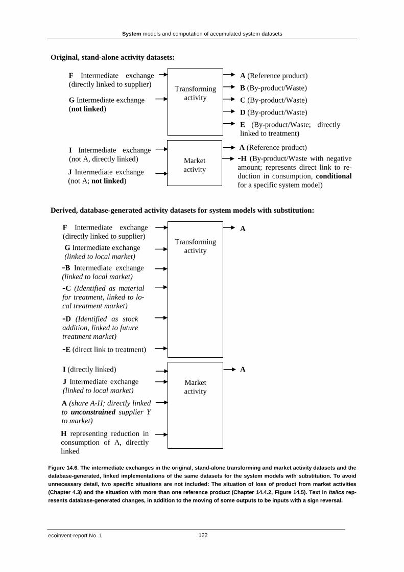
System models and computation of accumulated system datasets
ecoinvent-report No. 1 122
Figure 14.6. The intermediate exchanges in the original, stand-alone transforming and market activity datasets and the
database-generated, linked implementations of the same datasets for the system models with substitution. To avoid
unnecessary detail, two specific situations are not included: The situation of loss of product from market activities
(Chapter 4.3) and the situation with more than one reference product (Chapter 14.4.2, Figure 14.5). Text in italics rep-
resents database-generated changes, in addition to the moving of some outputs to be inputs with a sign reversal.
H representing reduction in
consumption of A, directly
linked
B (By-product/Waste)
A (Reference product)
C (By-product/Waste)
D (By-product/Waste)
G Intermediate exchange
(not linked)
E (By-product/Waste; directly
linked to treatment)
Market
activity
A (Reference product)
-H (By-product/Waste with negative
amount; represents direct link to re-
duction in consumption, conditional
for a specific system model)
I Intermediate exchange
(not A, directly linked)
J Intermediate exchange
(not A; not linked)
Original, stand-alone activity datasets:
Transforming
activity
Derived, database-generated activity datasets for system models with substitution:
F Intermediate exchange
(directly linked to supplier) A
-C (Identified as material
for treatment, linked to lo-
cal treatment market)
G Intermediate exchange
(linked to local market)
Market
activity
A I (directly linked)
Transforming
activity
-D (Identified as stock
addition, linked to future
treatment market)
-E (direct link to treatment)
J Intermediate exchange
(linked to local market)
A (share A-H; directly linked
to unconstrained supplier Y
to market)
-B Intermediate exchange
(linked to local market)
F Intermediate exchange
(directly linked to supplier)

System models and computation of accumulated system datasets
ecoinvent-report No. 1 123
Figure 14.7. The database-generated, linked, allocated implementations, derived from the original, stand-alone trans-
forming and market activity datasets shown in Figure 14.6. To avoid unnecessary detail, the situation of
loss of product from market activities (Chapter 4.3) is not included. Also not shown, are any additional by-
products from treatment activities, which would imply additional allocated instances of the transforming
activity. Text in italics represents database-generated changes, in addition to the moving of some outputs
to be inputs with a sign reversal.
In system models with substitution, by-products that can immediately – without further treatment –
substitute a reference product as an input to an activity (output B in Figure 14.6; identified by the da-
tabase service layer as a non-reference output which is the reference product of another activity in the
same geographical area) are moved to be negative inputs of the same activity and linked to the local
markets in the same way as described in the preceding paragraph for any other intermediate input. A
negative input implies a reduction in output from the market and therefore a reduction in (displace-
ment of) the other activities that supply the by-product to the market.
In system models with partitioning, a new allocated dataset is generated for each such by-product B
(by-product/waste C, D and E are identified as materials for treatment). The allocation procedure is
described in Chapter 14.4.1. The cumulative LCI results (see Chapter 4.15) of the multi-product activ-
ity (before allocation) are not available as ecoinvent LCI results. The allocated datasets have the same
activityID as the original dataset, which implies that the product name is required to distinguish the
allocated datasets from each other. For recycled products (by-products from treatment activities and
speciality productions), cumulative LCI results are not available for the allocated results before ag-
gregation, but only for the aggregated, partitioned activities. These aggregated, partitioned activities
have the same activityID as the original treatment activity or speciality production, which implies that
the product name is required to distinguish the allocated datasets from each other.
In the original market activities, the inputs of the reference product (product A in figure 14.6) are not
specified. These inputs are added by the database service layer: Based on the geographical area speci-
-E
(linked)
-D
(linked)
-C
(linked)
)
F
(linked)
Derived, database-generated activity datasets for system models with partitioning:
F Intermediate exchange (di-
rectly linked to supplier)
A
G Intermediate exchange
(linked to local market)
Market
activity
A I (directly linked)
Transforming
activity, allo-
cated for A
B
G
(linked)
J Intermediate exchange
(linked to local market)
A (share of; directly linked
to supplier X to market)
A (share of; directly linked
to supplier Y to market)
Transforming
activity, allo-
cated for B
-C (Identified as material
for treatment, linked to lo-
cal treatment market)
-D (Identified as stock
addition, linked to future
treatment market)
-E (direct link to treatment)

System models and computation of accumulated system datasets
ecoinvent-report No. 1 124
fied for each market activity, the database service layer first identifies the transforming activities that
are located within this geographical area. For the system models with linking to average current sup-
pliers, an input to the market is then added for each transforming activity (links to suppliers X and Y
in Figure 14.7). For system models with linking to unconstrained suppliers, an input is added only for
those transforming activities that are unconstrained (supplier Y in Figure 14.6), which are those for
which the product is a reference output (i.e. not a by-product, since the amount of a by-product is per
definition constrained by the corresponding reference products), and which has a technology level
(see Chapter 5.5) corresponding to the specific rule for the particular system model, see Chapter 14.6.
For both types of models, the amounts of inputs are added in proportion to the available production
volumes of the transforming activities included.
In system models that take into account constrained markets, any conditional exchanges (negative
output -H in Figure 14.6), representing reductions in consumption of the specific market output (see
Chapter 11.4), are moved to be positive inputs to the market activity, and are subtracted from the
amount of the reference product A before the remaining amount of market output is distributed over
the unconstrained suppliers, as described in the preceding paragraph. The market output, which stays
the same, is thus balanced by an input represented by that of the conditional exchange and the re-
mainder from any unconstrained suppliers.
[Changes relative to ecoinvent version 2: In version 2, all links between activity datasets were hard
links, added by the data providers. The new feature of database-generated links allows a more flexible
updating of the database, since all links can be automatically updated after the addition of new da-
tasets, and the data provider does not need to consider linking datasets specifically. The modelling of
materials for treatment is now more consistent. The option to produce implementations of the data-
base with system models with substitution is new.]
14.6 Models with substitution in the ecoinvent database
14.6.1 The “Substitution, consequential, long-term” model
The ‘Substitution, consequential, long-term’ model (short name: ‘Consequential’) is a system model
intended to reflect the consequences of small-scale, long-term decisions, by taking into account the
constraints that are applicable at this scale and time horizon. The scale and time horizon are relevant
because they delimit what suppliers, markets, products and technologies can be affected by the deci-
sion, and which should therefore be included in the system model.
A small-scale decision is defined as a decision that does not affect the determining parameters of the
overall market situation, i.e., the direction of the trend in market volume and the constraints on and
production costs of the involved products and technologies. The consequences of the decision can
thus be assumed linearly related to the size of the change and both an increase and a decrease in pro-
duction volume will affect the same processes. As shown by Mattsson et al. (2001), even a change in
the annual electricity demand by 1 TWh can still be regarded as small (marginal), since it affects the
same technologies as a change of 1 kWh, which means that the effects are linearly related to the size
of the change. The typical decisions studied by LCA can therefore be said to be small-scale.
The time horizon of a decision is defined as long-term if it affects capital investment (installation of
new machinery or phasing out of old machinery) as opposed to short-term decisions that affect only
capacity utilisation, but not capacity itself. However, even the effect of small, short-term decision can
seldom be limited to the short-term perspective, since each individual short-term purchase decision
will contribute to the accumulated trend in the market volume, which is the basis for decisions on cap-
ital investment (long term changes). This is obvious in free market situations (where market signals
play a major role when planning capacity adjustments) with a short capital cycle (fast turnover of cap-

System models and computation of accumulated system datasets
ecoinvent-report No. 1 125
ital equipment, as for example, in the electronics and polymer industries), but it is also true for mar-
kets with a long capital cycle (as for example, in the building and paper industries).
If a long-term investment is planned and announced well in advance of its implementation (as for ex-
ample, the installation of a new pipeline), it may involve only long-term effects, namely the effects
from installation and production on newly installed capacity. But such planned decisions are the ex-
ception. Most decisions will also lead to some immediate short-term effects, affecting the existing ca-
pacity, while at the same time affecting investments decisions and in the long run affecting the pro-
duction from this newly installed technology. Since the technology affected in the short term will of-
ten be old technology (the least competitive technology which typically has a low capacity utilisation
compared to newly installed technology) while the technology affected in the long term will often be
modern technology, long-term product substitutions may often be seen to affect a mix of technologies
(Mattsson et al. 2001). However, the short-term effect will typically be negligible compared to the
long-term effect, simply because the long-term effect is typically more permanent, while the short-
term effect only lasts until the next capacity change.
Consider a factory in which several production lines exist, some using an older technology, which is
more polluting and more expensive to run, and some with a new technology (less polluting, less costly
to run). Small, short-term fluctuations in demand will affect the capacity utilisation of the production
line with the older technology (since this is the most costly to run), while the line with the new tech-
nology will be utilised as much as possible, and will therefore not be affected. If the demand increases
beyond what can be covered by the current capacity, new machinery will be installed, and here the
factory may choose to install the newest technology even though it is more costly to acquire, or it may
decide to buy a cheaper, but more polluting technology. Whatever the choice, this can be said to be
the long-term result of the change in demand and the additional environmental exchanges from the
factory are now those coming from the newly installed machinery. It is therefore reasonable to ascribe
these exchanges to the change in demand. Once the new machinery has been installed, further changes
in short-term demand will still affect the older technology (since this is still the most costly to run). It
is important to understand that even though the short-term fluctuation constantly will affect the older
technology in the short-term, it is the accumulated changes in the short-term demands that make up
the long-term changes, which eventually lead to the installation of the new machinery. The long-term
effect of the demand is therefore the additional exchanges from the newly installed technology, and
the short-term effects can be seen as a mere background variation for this long-term effect. Thus, the
long-term effect should also be guiding for decisions that at first sight appear short-term, such as indi-
vidual purchase decisions, and the product declarations that support such decisions.
The ‘Substitution, consequential, long-term’ model generally assumes full elasticity of supply, just
like the models with linking to average current suppliers. This means that if the demand increases
with one unit, the producers will react by increasing their supply with one unit, and conversely when
the demand decreases. This makes it straightforward to trace the changes in the product system up-
stream, simply by following the increases in outputs of the upstream activities required to satisfy the
increases in demand of the downstream activities.
The assumption of full elasticity of supply is in accordance with the theoretically expected long-term
result of a change in demand on a unconstrained, competitive market, where there are no market im-
perfections and no absolute shortages or obligations with respect to supply of production factors, so
that production factors are fully elastic in the long term, and individual suppliers are price-takers
(which means that they cannot influence the market price), so that the long-term market prices are de-
termined by the long-term marginal production costs (implying that long-term market prices, as op-
posed to short-term prices, are not affected by demand).
When suppliers are constrained or markets are imperfect (so that producers can influence the market
prices), the assumption of full elasticity of supply should be modified.
Because the ‘Substitution, consequential, long-term’ model considers long-term changes, the rule for
the technology level of unconstrained suppliers depends on the market trend. If the market is generally

System models and computation of accumulated system datasets
ecoinvent-report No. 1 126
increasing, stable, or slowly decreasing (at a rate less than the average replacement rate for the capital
equipment), new capacity must be installed, typically involving a modern, competitive technology,
and any change will affect the decision on this capacity adjustment. In a market that decreases rapidly
(at a higher pace than what can be covered by the decrease from regular, planned phasing out of capi-
tal equipment) the affected suppliers will typically be the least competitive (often using an older tech-
nology).
The replacement rate for production equipment is determined as the inverse of the estimated lifetime
of the equipment. For the ‘Substitution, consequential, long-term’ model of the ecoinvent database, a
general lifetime of 30 years and a consequent rate of replacement of 3.33% annually is applied. The
market trend is automatically identified by the ecoinvent database service layer using the market da-
tasets with current average suppliers to compare the production volume for the current year with the
same dataset covering a period 3 years later. If a dataset covering the period 3 years later does not ex-
ist, the following datasets are used for the comparison, in order of priority: 3 years into the past, 4
years into the past, most recent past year, assume stable market without comparing to any other year.
Thus, when the production volume of the reference product is decreasing more than 3.33% annually,
the activity is identified as unconstrained if its technology level is “Old”, and when the production
volume of the reference product is decreasing less than 3.33% annually, increasing, or stable, the ac-
tivity is identified as unconstrained if its technology level is “Modern”. If there are no supplying ac-
tivities with the required technology setting, the requirement for “Modern” is replaced by ”New”,
and “Old” is replaced by “Outdated”, and if these do not exist, by the option “Current”.
In the ecoinvent database, market constraints are modelled by the use of conditional exchanges, see
Chapter 11.4, i.e. exchanges that are only activated for a specified system model, and which repre-
sents the share of the demand that is not met by increased supply, but which instead is coming from a
reduction in specified consumption activities. In general, the ‘Substitution, consequential, long-term’
model does not apply empirical elasticities, but only considers absolute constraints, as described in
Chapter 11.4.
In the ‘Substitution, consequential, long-term’ model, a joint production activity can only have one
reference product, except if there are more products from the activity that have no alternative produc-
tion routes. This follows from the assumption that suppliers are price-takers (which means that they
cannot influence the market price), so that the long-term marginal production costs of the alternative
production routes for the respective products provides a constraint on the long-term market prices of
the products, and thus on their contribution to the overall revenue of the joint production activity.
Thus, a change in demand for a specific joint product with an alternative production route will not
lead to a change in its (long-term) price and the change in demand will therefore not affect the overall
(long-term) revenue of the joint production activity.
The products that are defined as reference products in the ecoinvent database before any system mod-
elling (system model undefined) are also the reference products of the ‘Substitution, consequential,
long-term’ model. Only for other consequential system models (not currently implemented, see Chap-
ter 14.6.3) it may be relevant to define additional conditional reference products.
The system model ‘Substitution, consequential, long-term’ corresponds to the model described as ap-
plicable for “goal situation B for meso/macro-level decision support” in the ILCD Handbook (EC
2010), and is the one recommended by the ecoinvent Centre for consequential LCA modelling. As ar-
gued above, this model is also applicable to study the effect of small, short-term decisions, since each
individual short-term decision contributes to the accumulated trend in the market volume, which is the
basis for decisions on capital investment.
14.6.2 Substitution, constrained by-products
The ‘substitution, constrained by-products’ model (short name: ’substitution, ILCD A’) is a system
model [Not available at the time of release of version 3.0 of the ecoinvent database] where the on-

System models and computation of accumulated system datasets
ecoinvent-report No. 1 127
ly constraint taken into account is that the volume of a by-product per definition is constrained by the
corresponding reference product. Technology constraints are not taken into account. The inputs to
each market activity are therefore modelled as the market mix, excluding the by-products. This im-
plies that the inputs are coming from all those transforming activities within the geographical area of
the market activity, which have the market product as a reference product, in proportion to their
available production volume. Constrained markets are only applied for situations of more than one
reference product, as described in Chapter 14.4.2, and in case of markets where all inputs are by-
products.
Thereby, this system model corresponds to the model described as applicable for “goal situation A for
micro-level decision support” in the ILCD Handbook (EC 2010).
14.6.3 Outlook: Other models with substitution
The ecoinvent database does not currently provide other models with substitution than the above de-
scribed. However, the flexibility of the database structure allows the creation of other such models if
desired. Some reflections on other possible models are provided here.
Large-scale decisions affect the overall market situation, and therefore may bring into play new sup-
pliers, new markets, or even new products and technologies. Different large-scale decisions may af-
fect different markets, and it is therefore impossible to provide a generally applicable background da-
tabase for large-scale decisions. However, the datasets in the ecoinvent database may be modified by
the users to model specific large-scale changes, involving changes in market trends etc.
A system model for pure short-term effects of small, short-term changes could be constructed. As the
short term per definition does not involve capacity changes, many more production factors would be
constrained in such as system model. Only effects within the existing production capacity, including
reduction in current capacity would be included, and “old” technology would be the rule for the tech-
nology level of unconstrained suppliers, without any relation to the market trend. However, the results
of such a model would only be of interest in markets where no capital investment is planned (for ex-
ample, industries in decline), or where the market situation has little influence on capacity adjust-
ments (monopolised or highly regulated markets, which may also be characterised by surplus capaci-
ty). An example of a substitution with a short-term effect only would be an isolated decision to re-
move heavy metals from the components of a product, which – all other things equal – would not in-
volve capital investment in the metal industry, since heavy metals are already being phased out.
It would also be possible to construct a system model that introduced additional market elasticities via
the conditional exchanges, see Chapter 11.4. Thus, the inclusion of more elements from equilibrium
modelling would be possible. Research is ongoing at the ecoinvent Centre to investigate these options.
Both for such system models and for the modelling of large-scale changes the option to add more
conditional reference products is of interest.

System models and computation of accumulated system datasets
ecoinvent-report No. 1 128
14.7 Models with partitioning in the ecoinvent database
14.7.1 Revenue allocation
In the revenue allocated system model, the property “price” is used as allocation property. When mul-
tiplied by the amount of the outputs, the resulting values represent the revenues to the activity from
each output. When expressed relative to the total revenue, these values are the allocation factors, rep-
resenting the share of the other exchanges of the activity to be allocated to each output. Figure 14.8
provides an example of an allocation by revenue, with the allocation factors 9 and 1, based on the
amounts 1 kg and 0.5 unit, and the prices 9 EUR/kg and 2 EUR/unit, respectively.
Figure 14.8. Numerical example of an allocation by revenue.
14.7.2 Dry mass allocation (for mass flow analysis; not for LCA)
In the dry mass allocated system model [Not available at the time of release of version 3.0 of the
ecoinvent database], the property “dry mass” (DM) is used as allocation property. When multiplied
by the amount of the outputs, the resulting values represent the dry mass of each output. When ex-
0.5 unit product Y
0.5 kg resource R
1.7 kg product Z Multi-output
activity
1 kg product X; price 9 EUR/kg
0.5 unit product Y; price 2 EUR/unit
0.2 kg emission E
Total revenue (EUR): 1* 9 + 0.5 * 2 = 9 + 1 = 10
Before allocation:
0.5 * 9/10 = 0.45 kg
resource R
1.7 * 9/10 = 1.53 kg
product Z
Multi-output
activity, al-
located for
X
1 kg product X
0.2 * 9/10 = 0.18 kg emission E
After allocation:
0.5 * 1/10 = 0.05 kg
resource R
1.7 * 1/10 = 0.17 kg
product Z
Multi-output
activity, al-
located for
Y 0.2 * 1/10 = 0.02 kg emission E

System models and computation of accumulated system datasets
ecoinvent-report No. 1 129
pressed relative to the total dry mass balance of the activity, these values are the allocation factors,
representing the share of the other exchanges of the activity to be allocated to each output.
Note that this allocation is performed to all outputs with mass, including exchanges to the environ-
ment, in order to achieve a complete allocation that can be applied for mass flow analysis. It is not a
mass allocation to the products alone, as described in older LCA literature. The model is relevant for
investigating the origin of the mass included in a specific product, but not the mass of individual ele-
ments. It is not appropriate for investigating the total mass required to produce a specific product. For
such an investigation, we recommend the model ‘Substitution, consequential, long-term’ (Chapter
14.6.1) or the ‘Allocation, ecoinvent default’ model (14.7.4).
Figure 14.9 provides an example of the dry mass allocation, using the same example as for revenue
allocation.
Figure 14.9. Numerical example of an allocation by dry mass. Note that in order to achieve a complete allocation that
can be applied for mass flow analysis, allocation is made to all outputs with dry mass. The mass balance is
maintained for each activity, also after allocation. Allocation to emission E is not shown in the Figure. This
is not a mass allocation to be applied for LCA.
It should be noted that in a mass allocated system, no exchanges will be allocated to products without
mass, such as electricity and services. In the ecoinvent database, this also affects infrastructure prod-
ucts, since these are modelled as services providing production capacity.
0.5 unit product Y
0.5 kg resource R;
DM 1 kg/kg
1.7 kg product Z;
DM 1 kg/kg Multi-output
activity
1 kg product X; DM 1 kg/kg
0.5 unit product Y; DM 2 kg/unit
0.2 kg emission E; DM 1 kg/kg
Total dry mass (kg): 1* 1 + 0.5 * 2 + 1 * 0.2 = 1 + 1 + 0.2 = 2.2
Before allocation:
Multi-output
activity, al-
located for
X
1 kg product X
After allocation:
0.5 * 1/2.2 = 0.23 kg
resource R
1.7 * 1/2.2 = 0.77 kg
product Z
Multi-output
activity, al-
located for
Y
1.7 kg product Z;
DM 1 kg/kg
0.5 * 1/2.2 = 0.23 kg
resource R
1.7 * 1/2.2 = 0.77 kg
product Z
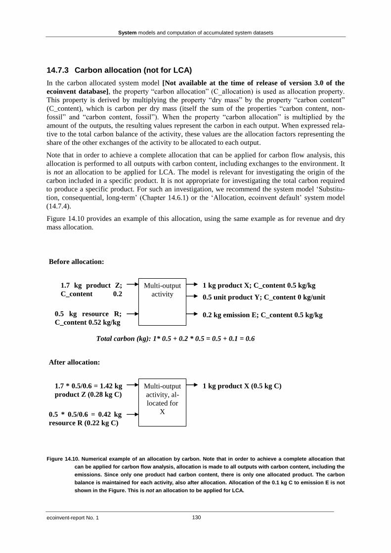
System models and computation of accumulated system datasets
ecoinvent-report No. 1 130
14.7.3 Carbon allocation (not for LCA)
In the carbon allocated system model [Not available at the time of release of version 3.0 of the
ecoinvent database], the property “carbon allocation” (C_allocation) is used as allocation property.
This property is derived by multiplying the property “dry mass” by the property “carbon content”
(C_content), which is carbon per dry mass (itself the sum of the properties “carbon content, non-
fossil” and “carbon content, fossil”). When the property “carbon allocation” is multiplied by the
amount of the outputs, the resulting values represent the carbon in each output. When expressed rela-
tive to the total carbon balance of the activity, these values are the allocation factors representing the
share of the other exchanges of the activity to be allocated to each output.
Note that in order to achieve a complete allocation that can be applied for carbon flow analysis, this
allocation is performed to all outputs with carbon content, including exchanges to the environment. It
is not an allocation to be applied for LCA. The model is relevant for investigating the origin of the
carbon included in a specific product. It is not appropriate for investigating the total carbon required
to produce a specific product. For such an investigation, we recommend the system model ‘Substitu-
tion, consequential, long-term’ (Chapter 14.6.1) or the ‘Allocation, ecoinvent default’ system model
(14.7.4).
Figure 14.10 provides an example of this allocation, using the same example as for revenue and dry
mass allocation.
Figure 14.10. Numerical example of an allocation by carbon. Note that in order to achieve a complete allocation that
can be applied for carbon flow analysis, allocation is made to all outputs with carbon content, including the
emissions. Since only one product had carbon content, there is only one allocated product. The carbon
balance is maintained for each activity, also after allocation. Allocation of the 0.1 kg C to emission E is not
shown in the Figure. This is not an allocation to be applied for LCA.
0.5 kg resource R;
C_content 0.52 kg/kg
1.7 kg product Z;
C_content 0.2
kg/kg
Multi-output
activity
1 kg product X; C_content 0.5 kg/kg
0.5 unit product Y; C_content 0 kg/unit
0.2 kg emission E; C_content 0.5 kg/kg
Total carbon (kg): 1* 0.5 + 0.2 * 0.5 = 0.5 + 0.1 = 0.6
Before allocation:
0.5 * 0.5/0.6 = 0.42 kg
resource R (0.22 kg C)
1.7 * 0.5/0.6 = 1.42 kg
product Z (0.28 kg C)
Multi-output
activity, al-
located for
X
1 kg product X (0.5 kg C)
After allocation:

System models and computation of accumulated system datasets
ecoinvent-report No. 1 131
No exchanges will be allocated to products without carbon content, such as electricity and services,
including infrastructure products, see also under mass allocation. Special care must be taken when us-
ing these results.
14.7.4 “True value” allocation (ecoinvent default)
The system model with “true value” allocation (‘Allocation, ecoinvent default’; short name: ‘Alloca-
tion, default’) is a variant of the revenue allocated system model, introduced to correct for some prob-
lems identified in the latter approach.
One problem in revenue allocation is that prices may be influenced by market imperfections or regula-
tion that distorts markets, resulting in relative prices that have very little to do with the true, function-
al value of the products. An example of this is the price of heat as a joint product from electricity pro-
duction. Here, it is possible to argue that exergy, i.e. the ability of the products to perform work, is a
shared property of the two products that reflects the true, functional value of the products, and that in
a perfect market this would be reflected in the price of the products.
Another problem in revenue allocation is that applying average prices for one single year may result
in a very high annual variation in the allocation factors for some multi-product datasets. To correct for
this, the ecoinvent default allocation instead applies three-year, historical average prices in such situa-
tions.
In the ecoinvent default allocation, the allocation property is identical to the price, unless the property
“true value relation” (true_value_relation) is specifically provided in the original dataset (the dataset
with system model undefined). See Chapter 5.6.6 for examples of situations where the “true value”
has been applied. One important example is the use of exergy to allocate between electricity and use-
ful heat.
When the property “true value relation” (true_value_relation) is specifically provided, the “true val-
ue” of the output is calculated as the “true value relation” property * amount * sum of revenues for all
products, divided by the sum of “true value relation” property * amount for all products. In this way,
the total “true value” of an activity (i.e. the “true value” summed over all products) is always identical
to the total revenue of the activity (price * amount, summed over all products). Thus, the “true value”
allocation only re-distributes the overall revenue, but does not change it.
When expressed relative to the total revenue, the “true values” are the allocation factors, representing
the share of the other exchanges of the activity to be allocated to each output.
[Feature considered for implementation later: The system model ‘allocation, ecoinvent default’
includes also corrections of carbon balances (see next sub-Chapter).]
The system model ‘allocation, ecoinvent default’ is the system model recommended by the ecoinvent
Centre for attributional LCA modelling. It is intended as a consistent implementation of the approach
used for ecoinvent versions 1 and 2.
14.7.5 Allocation corrections
An allocation correction is two datasets that counterbalance each other, re-allocating one or more en-
vironmental exchanges, so that the resulting allocated product systems have correct mass balances for
the re-allocated exchanges.
[Feature considered for implementation later: Allocation corrections are currently only considered
for the system model ‘Allocation, ecoinvent default’, and for one exchange only, namely “carbon di-
oxide, from air”. The rationale for applying the corrections to carbon only is that for carbon, in con-
trast to most other elements, the same substance as both input (capture of carbon dioxide from air) and
output (carbon dioxide to air) has the same significant environmental impact pathway (change in the

System models and computation of accumulated system datasets
ecoinvent-report No. 1 132
atmospheric concentration).] Figure 14.11 illustrates how the allocation correction for carbon works
on the example from Figure 14.8 and 14.10.
All allocation corrections are added automatically by the database service layer.

System models and computation of accumulated system datasets
ecoinvent-report No. 1 133
Figure 14.11. The numerical example of an allocation by revenue from Figure 14.8, with the carbon contents from Fig-
ure 14.10. After allocation, the activity allocated for X misses an input of 0.05 kg of C, while the activity allo-
cated for Y has a surplus input of 0.05 kg of C. The allocation correction datasets remove the surplus input
from the activity allocated for Y and add it to the activity allocated for X, so that both allocated activities
balance for both revenue and carbon.
0.05 kg R; 0.026 kg C
0.5 unit product Y; price 2
EUR/unit; C_content 0 kg/unit
0.5 unit product Y; 0 kg C
Total revenue (EUR): 1* 9 + 0.5 * 2 = 9 + 1 = 10
Before allocation:
0.5 * 9/10 = 0.45 kg re-
source R; 0.234 kg C
1.7 * 9/10 = 1.53 kg
product Z; 0.306 kg C
Multi-output
activity, al-
located for
X
1 kg product X; 0.5 kg C
0.2 * 9/10 = 0.18 kg emission E;
0.09 kg C
After allocation:
0.5 * 1/10 = 0.05 kg re-
source R; 0.026 kg C
1.7 * 1/10 = 0.17 kg
product Z; 0.034 kg C
Multi-output
activity, al-
located for
Y 0.2 * 1/10 = 0.02 kg emission E;
0.01 kg C
0.5 kg resource R;
C_content 0.52 kg/kg
1.7 kg product Z;
C_content 0.2
kg/kg
Multi-output
activity
1 kg product X; price 9 EUR/kg;
C_content 0.5 kg/kg
0.2 kg emission E; C_content 0.5 kg/kg
0.5 unit product Y; 0 kg C
0.45 kg R; 0.234 kg C
1.53 kg Z; 0.306 kg C Multi-output
activity, al-
located for
X
1 kg product X; 0.5 kg C
0.18 kg emission E; 0.09 kg C
After allocation correction for carbon:
0.17 kg Z; 0.034 kg C Multi-output
activity, al-
located for
Y 0.02 kg emission E; 0.01 kg C
Allocation
correction
for carbon
0.1832 kg CO2
from air; 0.05
kg C
Allocation
correction
for carbon
- 0.1832 kg CO2
from air; - 0.05
kg C

System models and computation of accumulated system datasets
ecoinvent-report No. 1 134
14.7.6 Outlook: Other models with partitioning
The ecoinvent database currently only provides partitioned models with average current suppliers. It
is possible to generate partitioned models with e.g. average modern suppliers or using rules for ex-
cluding specific constrained suppliers, while still maintaining allocation as the procedure for dealing
with joint production.
A system model with 100% allocation to the reference product is currently considered for implemen-
tation, since comparing this to the system models with substitution would allow to identify and quan-
tify the accumulated effect of the substitutions.
Since allocation is by definition a normative exercise, the number of thinkable allocation properties
and allocation corrections is unlimited. The ecoinvent Centre can provide specific system model im-
plementations on demand.
14.8 Computing of LCI results
The ecoinvent database system uses matrix inversion to calculate accumulated system datasets (LCI
results), separately for each combination of time period, macro-economic scenario and system model
for which datasets are present in the database. Calculations are only made for full calendar years or a
number of calendar years. Calculations are made for the current year and any full calendar year there-
after for which both start date (01-01) and end date (12-31) are present in any dataset. Beyond the
years for which individual calculations are made, calculations are also made for longer time periods of
calendar years for which the start date (01-01) and end date (12-31) are present in a dataset. Calcula-
tions for historical time periods, i.e. prior to the current year, are only performed on demand. For the
basic database result presentation, only the calculation results for the current year are displayed, using
the most recent data available for each activity and geography.
The calculation of the cumulative LCI results uses only the linked, single-product datasets derived
from the unlinked, multi-product datasets, as described above.
A dataset for an activity can be represented using vector notation. A dataset vector consists of an up-
per part which specifies the links to other activity datasets (intermediate input to the activity per unit
of output of the activity, see a in the vector below) and a lower part which specifies the elementary
exchanges per unit of output of the activity, see b in the vector below. The vector includes m interme-
diate exchanges ai (inputs of products supplied by other activities) and n elementary exchanges bj (re-
sources, emissions, and other inventory entries).
All datasets in the ecoinvent database can be arranged so that each activity is represented by a column
in a matrix. Each row in the upper part of the matrix (the a part of each vector) then represents the in-
termediate inputs per unit of output of each activity, and the lower part of the matrix (the b part of
each vector) represents the elementary exchanges per unit of output of the activities.

System models and computation of accumulated system datasets
ecoinvent-report No. 1 135
All activity column vectors together form a matrix with a square intermediate transaction part A and
an elementary part B. The matrix includes m columns (l), i.e. one column per activity whereas the
number of activities is the same as the number of products (m intermediate exchanges).
Since all the datasets are directly linked, and all datasets have only one product output, the intermedi-
ate transaction part A of the matrix above is square. The inverse of the matrix can therefore be calcu-
lated to provide the matrix of cumulative demand C of the intermediate products required to produce
each product:
C includes m rows and m columns. Each column in C represents the cumulative demand of intermedi-
ate products (rows) per unit of supply of the activity.
The matrix of cumulative elementary exchanges D for each product is calculated as
D includes n rows (each row represents an elementary exchange) and m columns. Each column in D
represents the cumulative elementary exchanges per unit of supply of the activity.
For the numerical implementation of the matrix inversion, direct methods are usually applied that
make use of publicly available source code libraries. These methods base on the Gauss-elimination
and use the LU factorisation creating a lower left triangular matrix L and an upper right triangular ma-
trix U.
The factorisation is done with a partial pivot strategy in order to guarantee the numerical stability. Be-
cause the size of the real figures in the matrix A varies between 10-6
to 106 (and even more), the scal-
ing of rows and columns should be done in a way that all new figures are about in the same order of
magnitude.
For fully occupied matrices the calculation requirements are proportional to the third power of the
size (m) of the matrix. For sparse matrices as the ecoinvent matrix, the use of renumeration and elimi-
nation strategies helps to dramatically reduce the calculation effort. The use of partial pivoting and an
eventual rescaling of the matrix guarantee the numerical stability.
Nevertheless, computational capacity may make it necessary to place certain restrictions on the num-
ber of datasets included in the matrix calculations. If such restrictions on the matrix size become nec-
essary, the limitations will be applied to the geographical detail. First, transforming activities that
supply to the same market will be pre-aggregated before matrix calculation, and secondly markets
may be pre-aggregated, starting with products that have many small geographical markets.

User advice on the results
ecoinvent-report No. 1 136
15 User advice on the results
15.1 LCI, LCIA and LCA results
The ecoinvent database does not aim at providing full LCA information (i.e., including a complete
goal and scope, and interpretation phase) of all investigated products. In general the discussion of re-
sults is kept quite short or even missing.
The ecoinvent database also contains life cycle impact assessment (LCIA) results to facilitate the in-
terpretation of LCI results. Assumptions and interpretations were necessary to match current LCIA
methods with the ecoinvent inventory results. They are described in Frischknecht et al. (2007a). It is
strongly advised to read the respective chapters of the implementation report and the original reports
describing the LCIA methods before applying LCIA results. Impact assessment results are reported on
the basis of a final indicator (e.g. “eco-indicator 99, hierarchist/average, total”) as well as on the basis
of safeguard subjects (e.g. “human health”) and environmental topics (e.g. “ionising radiation”).
The data collected and compiled in the ecoinvent database are not primarily suited for direct compari-
sons. Waste management datasets for instance shall not directly be used for waste management policy
assessments (landfilling versus incineration), transport service datasets shall not directly be used for
transport systems comparison and farming systems (integrated, extensive or organic production) shall
not directly and solely be compared based on ecoinvent data. In all cases the systems for comparison
have to be thoroughly defined beforehand. Then it has to be checked which adaptation to the average
data investigated would be necessary to appropriately describe these systems according to the goals of
the study.
15.2 Legal disclaimer
The ecoinvent Centre shall not be liable for any material defects/damages, including consequential
damages, loss of income, business or profit, special, indirect or incidental damages due to the use of
ecoinvent database or any ecoinvent dataset. The ecoinvent Centre disclaims all warranties, expressed
or implied, including, but without limitation, the warranties of merchantability and of fitness for any
purpose of ecoinvent Database or any ecoinvent Dataset. The database user must assume the entire
risk of using the ecoinvent database or any ecoinvent dataset.
15.3 Choice of system model
The ecoinvent data are available in different implementations representing different system models.
The original stand-alone activity datasets, each representing a specific human activity as it can be ob-
served “in real life”, are represented by the system model:
Undefined
These are the unlinked, multi-product activity datasets that form the basis for all the other system
models. This is the way the datasets are obtained and entered by the data providers. These activity da-
tasets are useful for investigating the environmental impacts of a specific activity (gate-to-gate), with-
out regard to its upstream or downstream impacts.
When the activity datasets are linked into product systems, a choice of a system model has to be
made, providing the rules for linking the activity datasets into contiguous product systems, each one
isolated from the datasets of all other product systems.

User advice on the results
ecoinvent-report No. 1 137
Two classes of system models can be distinguished: System models with substitution (system expan-
sion) and system models with partitioning (allocation). Within each of these two classes, several in-
stances can be defined.
For use in consequential LCA studies that investigates the long-term consequences (i.e. the conse-
quences including changes in production capacity) of small-scale decisions (i.e. decisions that do not
change the overall market conditions), the ecoinvent Centre recommends the system model:
Substitution, consequential, long-term (short name: ‘Consequential’)
This use situation corresponds to the one described as “goal situation B for meso/macro-level decision
support” in the ILCD Handbook (EC 2010), as long as this is restricted to small-scale decisions, not
affecting the market trends. This system model uses substitution (also known as ‘system expansion’)
to substitute by-product outputs. It includes only activities to the extent that they are expected to
change in the long-term as a consequence of small-scale changes in demand, taking into account both
constrained markets and technology constraints.
Consequential system modelling can be defined as a linking of activities in a product system so that
activities are included in the product system to the extent that they are expected to change as a conse-
quence of a change in demand for the product. Most LCA studies are aimed at decision support in-
volving a choice or substitution between two product systems. Even studies of a single product are
typically later used in a comparative context. For example, in LCA studies for hot-spot-identification
and product declarations, what appears to be stand-alone assessments of single products have the ul-
timate goal to improve the studied systems, thus supporting decisions that involve comparisons:
If a hot-spot-identification of a current product identifies a number of improvement options, it is still
necessary to assess the environmental impact of implementing the improvements, namely the differ-
ence in impact between the improved and the current product, obtained as a result of adding the im-
proved product and removing the current product.
Product declarations are used by the customer to make a choice between several products, and the (in-
tended) effect of this choice is that more of the chosen product will be produced at the expense of the
competing products. Thus, the impact of the choice is obtained as a result of adding one unit of the
chosen product and removing the corresponding amount of the current average product.
However, there are application areas where consequential modelling is less relevant, and an attribu-
tional model may be more appropriate. For these applications, the ecoinvent Centre recommends the
system model:
Allocation, ecoinvent default (short name: ‘Allocation, default’)
This system model subdivides multi-product activities by allocating all flows relative to their ‘true
value’, which is the economic revenue corrected for some market imperfections and fluctuations. It
includes activities in proportion to their current production volume. [Feature considered for imple-
mentation later: This system model also applies corrections to maintain mass balances for carbon,
while other mass and monetary balances are not corrected for.]
Examples of application areas are:
Studies at a societal level, where the entire environmental impact of all human activities is
studied, with the aim of identifying areas for improvement, disregarding whether such im-
provements shall be sought through product-oriented policies or through direct regulation of
the individual activities. In such a situation, it would not be reasonable to limit the study to
those activities that can be affected by changes in demands, but to include all activities, also
those that are not linked to any consequential product system, and for which a policy-driven
improvement can only be achieved through direct regulation. One can argue that since the ob-
jective of such a study is not product-oriented, LCA is simply not the (only) relevant assess-
ment technique. An attributional model, where all activities in society are included in propor-
tion to a specific attributional rule, such as “true value”, would better reflect the objective of

User advice on the results
ecoinvent-report No. 1 138
such a study. Once improvement options are identified by such a model, those improvement
options that have upstream or downstream consequences can then afterwards be studied with
a consequential model. The IMPRO study on meat and dairy products (Weidema et al. 2008)
is an example of such an attributional study at the level of EU-27, where the identified im-
provement options were analysed with a consequential model.
Studies on environmental taxation, where the focus is less on the consequences of the tax, but
rather on who is to carry the burden. Often, studies on taxes or quota systems are performed
for a specific administrative area, and any consequences outside this administrative area are
discounted. Although the consequences of a tax on a product or an activity can be studied by
a consequential model, this model cannot say anything about the attribution of the tax and its
fairness. An attributional model, where all activities in society are included in proportion to
their perceived contribution to the taxed activity variable, whether or not this changes as a
consequence of the tax, would better reflect the objective of such a study.
Studies that seek to avoid blame or to praise or reward for past good behaviour, for example
avoiding blame that a specific controversial activity, such as nuclear power, occurs in the
product system, or rewarding producers that have invested in a praiseworthy technology such
as solar power. While a consequential model can answer the question whether the controver-
sial or praiseworthy activity changes as a consequence of buying the product, it cannot tell
how much of the controversial or praiseworthy activity exist in the product system. An attrib-
utional model, where activities are included in proportion to a specific attributional rule, for
example “true value”, would better reflect the objectives of such studies.
Outlook: In addition to the above database implementations recommended respectively for conse-
quential and attributional LCA studies, the ecoinvent database will also be available in separate im-
plementations for very specific application areas:
Substitution, constrained by-products (short name: ‘Substitution, ILCD A’)
This implementation is specifically provided for users that need to fulfil the requirements of the ILCD
Handbook (EC 2010) for the “goal situation A for micro-level decision support”. It consistently ap-
plies substitution (system expansion) for by-products, but substitutes with the market mix, excluding
the substituted by-products.
Allocation by revenue (short name: ‘Allocation, revenue’)
This system model includes activities in proportion to their current production volume and subdivides
multi-product activities by allocating all flows relative to the revenue generated by the outputs, using
annual prices as basis. The allocations may therefore fluctuate more than in the ‘ecoinvent default’
implementation where “true value” is used. However, this is the same modelling principle as applied
in many input-output analyses, and this system model is therefore the most appropriate implementa-
tion to compare with national direct requirement tables (“input-output” tables) using the industry-
technology model, and for creation of corresponding hybrid models.
Allocation by dry mass (short name: ‘Allocation, dry mass’)
This system model subdivides multi-product activities by allocating all flows relative to the dry mass
of the outputs. It includes activities in proportion to their current production volume. This implemen-
tation is applicable for mass flow analysis, since the dry mass balances are preserved, including the
mass leaving the product systems as emissions. This model can therefore be used to investigate exact-
ly how much of a specific mass input is contained in any product. It is not a mass allocation to the
products alone, as described in older LCA literature, and should not be used for Life Cycle Assess-
ments.
Allocation by carbon (short name: ‘Allocation, carbon)
This system model subdivides multi-product activities by allocating all flows relative to the carbon
content of the outputs. It includes activities in proportion to their current production volume. It is in-

User advice on the results
ecoinvent-report No. 1 139
tended for carbon tracing along supply chains, since the carbon balances are preserved, including the
carbon leaving the product systems as emissions. This model can be used to investigate exactly how
much of a specific carbon input is contained in any product. It is not an allocation to be applied for
LCA.
15.4 Uncertainty information
[Feature considered for implementation later: Resuming the display of uncertainty information for
the accumulated LCI results.]
The ecoinvent inventory result files contain quantitative and qualitative information about the uncer-
tainty of each individual elementary exchange. In many cases a simplified pedigree approach has been
used.
Uncertainty information is valuable to judge the overall variability of LCI results. Care must be taken
when using the uncertainty values in comparative assertions on the basis of LCI results because most
underlying uncertainty values are estimated.
The uncertainty values presented in the cumulative LCI results should not be used directly for LCA
case studies, since the uncertainty values of the individual exchanges and datasets are not independ-
ent. For a correct uncertainty assessment for the modelled LCA case study, the uncertainty infor-
mation on a unit process level is required. A simulation (e.g. Monte Carlo) based on the case study’s
LCI raw data is required to correctly assess the uncertainty in the LCI results. Some of the commer-
cially available LCA software are able to perform such project-specific simulations.
The minimum and maximum values of elementary exchanges reported in the LCI results of the ecoin-
vent database shall not be added to total emissions into a compartment because the sum of all mini-
mum and maximum values, respectively, does not correspond to the minimum and maximum values
determined with a Monte Carlo simulation.
15.5 How to reproduce and quote ecoinvent data in case studies
The ecoinvent terms of use state that:
"Licensee is not entitled to use the ecoinvent Database or the ecoinvent Dataset by preparing ex-
tracts, or for any further commercial purposes.
Licensee is not entitled to reproduce, disseminate or publicly display any significant portions of the
ecoinvent Database or the ecoinvent Datasets.
Licensee is not entitled to sell, rent, lease, loan, distribute, export, import, act as an intermediary or
provider, or grant any kind of licence rights to third parties with regard to the ecoinvent Database,
the ecoinvent Dataset or any portions thereof.
Licensee is not entitled to undertake, cause, permit or authorize the modification, creation of deriva-
tive works, translation, reverse engineering, decompiling, disassembling or hacking of the ecoinvent
Database the ecoinvent Dataset or any part thereof except to the extent permitted by law.”
It means that ecoinvent LCI raw data and results and LCIA results (either directly downloaded from
the ecoinvent database or calculated with ecoinvent LCI results and the factors downloaded from the
ecoinvent database) shall not be reproduced in other LCA case studies. Contribution analyses may in-
clude graphical representation of the share of ecoinvent activities on the total LCA results (e.g., the
contribution of energy supply to the total burdens of manufacturing a mobile phone). Hereby the pos-
sibilities to recalculate the exact LCI and LCIA results of an ecoinvent dataset shall be prevented as
much as possible.

User advice on the results
ecoinvent-report No. 1 140
The ecoinvent data shall generally be quoted by including the exact version number and system model
of the database applied. Additional reference may be made to the respective location of the datasets if
specific datasets have been used. If the ecoinvent database and its contents are cited as a whole the
following format is recommended:
ecoinvent Centre 2013 ecoinvent Centre (2013) ecoinvent data v3.0. Swiss Centre for Life Cycle Inventories, St. Gallen, retrieved from: www.ecoinvent.org.

Contributing to the ecoinvent database
ecoinvent-report No. 1 141
16 Contributing to the ecoinvent database
16.1 Individual data providers
Anyone can contribute to the ecoinvent database. To supply new data or to make larger changes to ex-
isting datasets, prospective data providers should download (from www.ecoinvent.org) the ecoEditor
software that supports the editing process.
The dataset(s) that you wish to edit can be downloaded to your harddisk from the production version
of the ecoinvent database. From the dataset it can be seen if the dataset has an active author assigned,
see Chapter 16.3. If you intend to edit or update an existing dataset with an active author, it may be a
good idea to inform the active author of your intentions/suggestions, e.g. by using the dataset talk
page, see Chapter 16.4.
Once you have finished editing your dataset(s), you can upload it/them for pre-validation and/or for
review directly from the ecoEditor, when on-line.
Outlook: If you have restrictions on allowing the ecoEditor on-line access (e.g. a firewall), it is con-
sidered that you may submit your dataset(s) via the ecoinvent web-site, using your web-browser. This
feature has not yet been implemented.
When submitting a dataset, the data provider confirms ownership to the data, and transfers the right to
use to the ecoinvent Centre.
We particularly encourage LCA practitioners to share their data though the ecoinvent database. The
new data collected for a specific LCA could very well be useful for others. An added benefit is that
both you and others will be able to reuse the supplied data in other contexts, fully embedded in the
richness of the ecoinvent database.
We also encourage industry associations, individual enterprises and public and private organisations
to provide data for their own activities. For larger data collection projects, the ecoinvent Centre offers
support for planning and fundraising.
16.2 National data collection initiatives
The ecoinvent Centre cooperates with national data collection initiatives (NDIs) to provide national
versions of the ecoinvent database, fully integrated with the rest of the World.
The ecoinvent Centre provides free of charge the necessary infrastructure for validation and publish-
ing of the national data as part of the ecoinvent database. The ecoinvent Centre provides an in-kind
payment of free ecoinvent licenses to all active in the NDIs, and supports the NDIs with annual finan-
cial contributions.
The NDI proposes one or more editors to be responsible for reviewing datasets for geographical con-
sistency before uploading to the ecoinvent database, irrespective of whether the datasets result from
the national data collection programme or is provided by a third party. The ecoinvent Centre has the
final responsibility for appointing and supervising editors. Editors are paid directly by the ecoinvent
Centre in accordance with the ecoinvent procedures for such payments.
The NDI retains copyright and the right to license the collected data to third parties, while providing
the collected data for publication in the ecoinvent database. Data provided to the ecoinvent Centre are
provided with the permission to the ecoinvent Centre to publish these data.

Contributing to the ecoinvent database
ecoinvent-report No. 1 142
16.3 Active and passive authorship
The ecoinvent Centre regards data providers as authors of the supplied datasets. Thus, editors cannot
make corrections to the datasets, but only comment back to the data provider, asking the data provider
to make corrections. This is also the case after publication of the dataset, if the editor or a third party
discovers an error in a dataset, or suggests improvements.
When submitting a dataset, the data provider (author) chooses to be either an active author, i.e. re-
sponsible for future modifications of the dataset, or a passive author, i.e. recognised as author of the
submitted version, but not involved in any further maintenance or modifications of the dataset.
If a dataset has an active author, prospective data providers are recommend to submit comments to the
active author via the discussion boards on the Editor's pages before submitting changes or updates as
full datasets.
Active authors are automatically informed when there are news on the talk page related to the dataset
and if another data provider submits a modified version of the dataset. In the latter situation, the active
author is given 14 days to comment on the suggested modifications, and to indicate whether she/he
wishes to maintain authorship of the dataset, before the dataset is passed on to the activity editor.
Failure to react is interpreted as acceptance that authorship and responsibility for the modified dataset
is transferred to the modifying data provider. The original author is informed of this, and has the op-
tion to resume responsibility as long as the modified dataset is not yet published. This does of course
not affect the authorship of the original, unmodified dataset, which remains accessible in the older
versions of the database.
An author can always decide to withdraw from this active role, in which case the responsibility for re-
sponding to questions and suggestions for modifications of the dataset lies exclusively with the editor.
If modifications are to be made in a dataset where the author has withdrawn from active participation,
the person who modifies the dataset becomes the author of the new modified dataset. Appropriate
credits to the previous author(s) are included in the new dataset.
An author of a dataset cannot at any time be editor for the same dataset. Instead, a co-editor will be
the editor for this dataset. This applies to the situation where an editor contributes datasets within his
own editorial area, and also when an editor is forced to make corrections to a dataset for which the ac-
tive author has withdrawn. In the latter situation, the editor may ask another author to make the re-
quired changes and remain as editor, or – when this is not possible or appropriate – perform the
changes and thus resign as editor for this particular dataset.
In the situation that an active author refuses to make changes that are seen by the editor as essential
for the scientific validity of a dataset, the editor may allow a new version of the dataset with another
author. As always, the old dataset remains in the old version of the database. Such cases, where an ed-
itor suggests dismissing an active author, will always be handled by the ecoinvent database manage-
ment, which will express its view on the matter. Both the editor and the author will also have the pos-
sibility to consult the ecoinvent database management before the decision is made to transfer the re-
sponsibility to a new author.
16.4 Reporting errors / suggesting improvements
If you discover an error in an ecoinvent dataset, or wish to suggest an improvement, but are not inter-
ested in supplying the corrected or improved dataset yourself, you may submit your observations via
the ecoinvent discussion boards for the dataset in question on the Editor's pages at
www.ecoinvent.org. The ecoinvent discussion boards on the Editor's pages are also open for placing
questions, which may be answered by the authors, the editors or any other interested party.
Active authors and the editor of an ecoinvent talk page are responsible for ensuring a response to re-
ported errors, suggestions and questions within a reasonable time (typically 14 days).

Contributing to the ecoinvent database
ecoinvent-report No. 1 143
Discovered errors will be corrected in a next intermediate version of the database. Until then, known
errors are reported on the ecoinvent web-site, both on the relevant talk page and in the aggregated
“Known errors” page.

History of the ecoinvent database
ecoinvent-report No. 1 144
17 History of the ecoinvent database
17.1 The origin
Up to the late nineties, several public Life Cycle Assessment (LCA) databases existed in Switzerland,
partly covering the same economic sectors (Frischknecht et al. 1994, 1996; Gaillard et al. 1997; Ha-
bersatter et al. 1996, 1998; Künniger & Richter 1995). These databases were developed by different
institutes and organisations. Life cycle inventory data for a particular material or activity available
from these databases often did not coincide and therefore the outcome of an LCA were (also) depend-
ent on the institute working on it. Furthermore, the efforts required to maintain and update compre-
hensive and high quality LCA-databases are beyond the capacity of any individual institute.
At the same time, LCA received more and more attention by industry and authorities as one important
tool for e.g., Integrated Product Policy, Technology Assessment, or Design for the Environment. In
parallel with this increasing trend in LCA applications, the demand for high quality, reliable, trans-
parent, independent and consistent LCA data increased as well.
17.2 ecoinvent data v1.01 to v1.3
The first steps for the ecoinvent project were taken during the late 1990ties. The individual projects
for data harmonisation and compilation have been funded by the Swiss Federal Roads Authority
(ASTRA), the Swiss Federal Office for Construction and Logistics (BBL), the Swiss Federal Office
for Energy (BFE), the Swiss Federal Office for Agriculture (BLW), and the Swiss Agency for the En-
vironment, Forests and Landscape (BUWAL). The database software development was funded by the
Swiss Centre for Life Cycle Inventories and the salary for the project management by Empa and the
Swiss Centre for Life Cycle Inventories.
After the successful launch of ecoinvent data v1.01 in 2003, the work concentrated on an extension
and revision of the contents resulting in the release of version 2.0 in 2007.
17.3 ecoinvent data v2.0 to 2.2
The LCA-institutes in the ETH domain (Swiss Federal Institutes of Technology (ETH) Zürich and
Lausanne, Paul Scherrer Institute (PSI) Villigen, and Swiss Federal Laboratories for Materials Testing
and Research (Empa) in St. Gallen and Dübendorf) as well as the LCA-group of the Agroscope
Reckenholz-Tänikon Research Station (ART) in Zürich continued their co-operation in the Swiss
Centre for Life Cycle Inventories, the ecoinvent Centre.
Besides the institutions mentioned above the following consultants contributed with LCI data compi-
lation: Basler & Hofmann, Zürich, Bau- und Umweltchemie, Zürich, Carbotech AG, Basel, Chudacoff
Oekoscience, Zürich, Doka Life Cycle Assessments, Zürich, Dr. Werner Environment & Develop-
ment, Zürich, Ecointesys - Life Cycle Systems Sarl., Lausanne, ENERS Energy Concept, Lausanne,
ESU-services Ltd., Uster, Infras AG, Bern and Umwelt- und Kompostberatung, Grenchen. Rolf
Frischknecht lead the ecoinvent management, Annette Köhler was in charge with Marketing and sales
and ifu Hamburg GmbH with software development and support.
By 2007, the ecoinvent database had become the most widespread and acknowledged life cycle inven-
tory database worldwide. This success was only possible because of the on-going support by Swiss
Federal Offices and European Organisations. In particular we wish to express our thanks to the Swiss
Federal Office for the Environment (FOEN - BAFU), the Swiss Federal Office for Energy (BFE) and
the Swiss Federal Office for Agriculture (BLW). We received further support from several associa-
tions, namely Alcosuisse, Biogas Forum Schweiz, Entsorgung und Recycling Zürich, Amt für Hoch-

History of the ecoinvent database
ecoinvent-report No. 1 145
bauten Stadt Zürich, Erdöl-Vereinigung, the European Photovoltaics Industry Association (EPIA) and
others. We wish to express our thanks for their valuable support.
In 2008, the management of the ecoinvent Centre was taken over by Bo Weidema, with Roland His-
chier as deputy manager, and the planning of version 3 was initiated, while at the same time publish-
ing additional data and corrections in the versions 2.1 and 2.2.
17.4 ecoinvent data v3.0
The cooperation of the ecoinvent institutes continued for the development of version 3, under the
leadership of Gerard Gaillard from Agroscope Reckenholz-Tänikon Research Station (ART). The sci-
entific management was performed by Bo Weidema, while the business management from 2012 was
passed on to Gregor Wernet. The staff of the ecoinvent Centre had in the meantime grown from one
full-time person to five. The cooperation with ifu Hamburg GmbH for software development and sup-
port was continued.
The development of version 3 of the ecoinvent database was possible exclusively from the funds ob-
tained from sales of licenses and substantial in-kind contributions of the above-mentioned LCA-
institutes in the ETH domain. We furthermore received funding for data collection from TetraPak.

Annex A. The boundary to the environment
ecoinvent-report No. 1 146
Annex A. The boundary to the environment
To distinguish human activities from their environment, two principles are followed in combination:
1) “The natural background”, i.e. to include everything that would not have occurred without the ac-
tivity, and to exclude anything that would have occurred even without the activity. The exclusion of
the natural background may be done implicitly, by simply ignoring it, but for transparency it may be
preferable to include the natural background phenomena in the activity description (or in a separate
description) and explicitly subtract them. This principle delimits the subject of LCA from the study of
natural phenomena, but does not in itself provide a delimitation between life cycle inventory (LCI)
and life cycle impact assessment (LCIA). Examples of application of this principle are:
Forest residues, such as branches and stubs left after harvesting, are excluded, because they would
anyway have decomposed, in situ, on the forest floor (although possibly at a different time). This
implies that only the wood actually harvested (and the management activities required to achieve
this) is seen as included in the forest activity and in the mass and carbon balance for this activity.
If the forest activity has an effect after the harvest, e.g. CO2 emissions from the soil after a clear-
cut, additional to those that would have occurred without the clear-cut, these are to be included in
the LCA.
The heavy metals and nutrients brought into an agricultural system by the management are to be
included, while the deposition from precipitation (whether from natural or human sources) are ex-
cluded. Likewise, the natural background leaching that would have occurred from the area, had it
been under natural climax vegetation, is excluded.
Indoor emissions from an activity are to be included, since they would not have occurred without
the activity.
Deposition of waste in a landfill, as well as littering, is included as an activity, since it would not
have occurred without human presence.
2) “Human management”, i.e. to include everything that takes place under human management and
exclude anything that takes place after human management has terminated. This principle is mainly
aimed at delimiting LCI (the human activity) from LCIA (the fate and exposure modelling and as-
sessment of e.g. the emissions from the activity). While this principle may at first appear simple, it
does not in practice provide a clear and practicable boundary between LCI and LCIA:
The CO2 emissions from the soil after a forest clear-cut do not take place under human manage-
ment. The human management leaves a disturbed soil (this could be seen as the “exchange to the
environment”), which then has these emissions. Nevertheless, it appears more practical to include
the CO2 emissions as emissions from the forestry activity (or a separate after-forestry activity), ra-
ther than to introduce disturbed soil as an environmental exchange.
Many fate models for pesticides take their starting point in the amount of pesticide applied to the
agricultural soil, although this clearly is within the sphere of human management and only the
amount of pesticide that reaches the surrounding environment (and possibly the soil after human
management terminates) are included in the final impact assessment (i.e. excluding the effect on
the flora and fauna of the agricultural soil while under human management).
Landfill emissions are included as elemental emissions also after the human management of the
landfill has terminated. If the principle of management was followed strictly, the landfill content
at the time of termination of human management should be reported as an exchange to the envi-
ronment, and the rest treated as part of the LCIA fate modelling. Since the fate models used would
not be different from those applied during human management, this would be a very unpractical
division.

Annex A. The boundary to the environment
ecoinvent-report No. 1 147
Following the principle of management, each individual type of litter (PET bottles, alu cans, etc.)
should be treated as an exchange to the environment. Although specific issues of littering (e.g. di-
rect harm to wildlife) may still need special treatment, a more practical solution would be to apply
a surface landfill model resulting in the traditional elemental emissions.
As it appears difficult to determine an unambiguous and practicable boundary between LCI and
LCIA, the ecoinvent database applies a pragmatic, exemplary approach, where the centrally managed
master list of elementary exchanges (available via www.ecoinvent.org and via the ecoEditor software)
provides the definition of the borderline between LCI and LCIA. This implies that all activities up to
the point where the listed emissions first occur are regarded as included as human activities, while the
remaining fate modelling is regarded as belonging to the LCIA. The ecoinvent Editor for Exchanges
with the environment is thus responsible for the smooth linking to the available LCIA methods, ensur-
ing that no gaps or overlaps occur between the LCI and the LCIA phases.

Annex B. Parent/child datasets (inheritance)
ecoinvent-report No. 1 148
Annex B. Parent/child datasets (inheritance)
[Note: In the context of the ecoinvent database version 3, inheritance is restricted to geograph-
ical inheritance, i.e. the creation of local child datasets from a global parent dataset. The ecoin-
vent Centre will perform experiments with temporal and scenario child datasets to investigate
the options for expanding the use of inheritance in future versions of the database.]
B.1 Reference datasets
A reference activity dataset is intended as a dataset that provides data close to the global average for
the activity for the most recent year for which data is available.
The reference settings applied in the ecoinvent database version 3 are:
Geography: Global
Time period: The most recent year (current year or earlier) for which a global dataset covering a
full calendar year is available (individually for each activity)
Macro-economic scenario: Business-as-Usual
Reference datasets are only defined for transforming and market activities, and are not available for
other special activity types.
B.2 Inheritance rules
The ecoSpold 2 data format is in itself not very restrictive in terms of which datasets are allowed to
inherit from which. In order to ensure consistency of the ecoinvent database, a number of further re-
strictions are therefore applied:
A child dataset always refers to a parent dataset with the same activity name as the child, using
the “parentActivityId” field of the ecoSpold format. Also the system model, activity type (unit
process or aggregated system, see Chapter 4.15) and special activity type (see Chapter 4.3) cannot
be changed from parent to child.
A child dataset differs from the parent dataset on one (and only one) of the settings for geography,
time period and macro-economic scenario.
Temporal child datasets (i.e. datasets with a time period setting different from the parent) and
macro-economic scenario child datasets (i.e. datasets with a macro-economic scenario setting dif-
ferent from the parent) are only allowed for time periods after the current calendar year, and can
only be created by the use of database-wide algorithms that are not dependent on a fixed reference
year. The addition of temporal and macro-economic child datasets can therefore only be added in
cooperation with the ecoinvent database administration, and not as individual datasets.
The inheritance is furthermore limited to the fixed sequence: Reference activity Geography child
Temporal child Macro-economic scenario child, with the exception that a Geography child may
keep its original parent (the corresponding global dataset) even after a more recent dataset has become
the reference activity dataset for this activity. This means that:
A geography child (i.e. a dataset with a geographical location setting different from the parent)
can only refer to a global dataset for the same time period as its parent and geography child da-
tasets can only be available for the reference year or earlier. Geographically specific datasets for
future years can be constructed from the most recent geographical child datasets as temporal child
datasets.

Annex B. Parent/child datasets (inheritance)
ecoinvent-report No. 1 149
A temporal child (i.e. a dataset with a time period setting different from the parent) can only refer
to a reference activity or the most recent geography child as its parent. Temporal child datasets
are only available for the reference scenario (Business-as-Usual). Temporal specific datasets for
other macro-economic scenarios are constructed from the temporal child datasets as macro-
economic scenario child datasets. This allows the construction of time series of datasets for any
activity, location and macro-economic scenario.
A macro-economic scenario child (i.e. a dataset with a macro-economic scenario setting different
from the parent) can only refer to a reference activity, the most recent geography child, or a tem-
poral child as its parent.
The fixed sequence implies that different geographies are allowed to have different temporal resolu-
tion and different developments over time, while all macro-economic scenarios using inheritance must
have the same geographical and temporal resolution, but can still have different developments over
geography and time.
This also means that inheritance is not used to model technologically similar datasets (e.g. lorries with
different capacities) outside the context of a geography child. Technologically similar datasets are in-
stead modelled with the use of variables, see Chapter 5.7. Ideally, the reference activity dataset is pa-
rameterised with the use of variables, before it is applied for inheritance.
In the ecoSpold 2 format, inheritance is implemented through the use of delta datasets that contain
only data on the inheritance and difference of the child as compared to a parent dataset, so that the ac-
tual child dataset only occurs when the delta dataset is combined with the inherited content from the
parent dataset.
The ecoSpold format distinguishes 5 ways in which data in a delta dataset is interpreted:
1. A blank field: The value from the parent activity dataset applies.
2. Filled-in content: The filled-in value applies, and the value from the parent activity dataset is ig-
nored.
3. In text fields of the string type, content may include the text {{PARENTTEXT}}, in which case
the field content from the parent activity dataset is included at this place in the filled-in text in the
child dataset.
4. In fields of the type TTextAndImage, content may include both {{PARENTTEXT}} and
{{text_variables}}. The latter represents a text variable defined in the parent dataset, which may
be redefined by the delta dataset while keeping the rest of the parent text intact. This allows easy
changes of text parts in child datasets.
5. In amount fields with corresponding mathematical relation fields, the latter may include the re-
served variable PARENTVALUE referring to the value of the parent dataset. For example, the
formula PARENTVALUE*0.5 halves the value of the parent amount field.
Additional advice for data providers:
When expressing an amount in a delta dataset, it is important to consider whether it is most relevant to enter the
child value as a fixed value (i.e. not relative to the parent), or whether the PARENTVALUE variable should be
used. When the PARENTVALUE relationship is used, it is important to consider whether the relationship is ad-
ditive or multiplicative. For example, a child value of 50 relative to a parent value of 100 can be expressed as
PARENTVALUE-50 or PARENTVALUE*0.5. It is important to consider what will happen to the child value if
the parent amount is changed. If there is no specific reason to assume an additive relation, the multiplicative rela-
tion should always be preferred. If the child value is believed to be more correct than any relative amount, e.g.
because it is a measured value, the child value should be entered as a fixed value that will not change with the
parent value. If the parent field is a mathematical relationship, it is often relevant to re-use this mathematical rela-

Annex B. Parent/child datasets (inheritance)
ecoinvent-report No. 1 150
tionship in the child dataset. It is important to use the comment fields to explain the rationale behind any entered
relationships.
When data for a specific local activity is available, it is recommended simultaneously to consider the global and
the local dataset for this activity and which specific data are most relevant to add to each of these datasets. It may
be most simple at first to create a stand-alone local dataset with the available data and in a second step split it up
in the global parent and the local child, which will then supersede the stand-alone dataset.
When submitting an edited version of a parent dataset, the consequences for the child datasets will be reviewed at
the same time as the edited parent dataset.

Annex B. Parent/child datasets (inheritance)
ecoinvent-report No. 1 151
Abbreviations
AOX Adsorbable Organic Halogen Compounds
BOD5 Biological oxygen demand in five days
CED Cumulative Energy Demand
CIF Cost Insurance and Freight
COD Chemical oxygen demand
CPC Central Product Classification
CV Coefficient of Variance
DM Dry matter
DOC Dissolved organic carbon
FOB Free On Board
GDP Gross Domestic Product
GLO Global
ID Identifier
IO Input Output (economic model)
ISO International Organization of Standardization
ISIC International Standard Industrial Classification
KML Keyhole Markup Language
LCA Life Cycle Assessment
LCI Life Cycle Inventory
LCIA Life Cycle Impact Assessment
NAICS North American Industry Classification System
NDI National Data collection Initiative
NPP Net Primary Productivity (NPP-C: Net Primary Productivity Carbon)
NMVOC Non-methane Volatile Organic Compound
PM10 Particulate matter with a diameter of less than 10 µm
PM2.5 Particulate matter with a diameter of less than 2.5 µm
ROW Rest-Of-World
SPOLD Society for the Promotion of Lifecycle Development (www.spold.org)
TCDD Tetra-chlor-dibenzo-dioxin
TOC Total Organic Carbon
TPM Total Particulate Matter
TDS Total Dissolved Solids
TSS Total Suspended Solids
UN United Nations
UUID Universally Unique Identifier
XML Extended Markup Language

Annex B. Parent/child datasets (inheritance)
ecoinvent-report No. 1 152
Standard terminology used in the ecoinvent network (glossary)
Accumulated system dataset: An activity dataset showing the aggregated environmental exchanges
and impacts of the product system related to one specific product from the activity.
Activity: The doing or making something. Example: "International Standard Industrial Classification
of All Economic Activities". Etymology: Latin: actio (“‘doing or making’”)
Activity class: Group of activities classified together under a heading in a statistical classification of
activities, such as ISIC.
Addition to stock: By-product or waste with a lifetime in excess of one year. See also under Infra-
structure.
Branded dataset: Dataset for a specific brand or a specific company, where the company or brand
name is specifically mentioned as part of the activity and/or product name.
By-product/Waste: Any activity output that is neither a reference product nor an exchange to the envi-
ronment. The ecoinvent database does not discriminate between by-products and
wastes.
Child dataset: Dataset that occurs when a parent dataset is combined with a delta dataset.
Conditional exchange: Exchange that is only activated for a specified system model.
Constrained activity: An activity that is limited in its ability to change its production volume in re-
sponse to a change in demand for its product.
Consumption mix: The output from a market activity.
Cost: The expenditure necessary to acquire a product or production factor.
Delta dataset: Dataset that contains information on the inheritance and difference of a child dataset as
compared to a parent dataset.
Determining product: See reference product.
Direct requirements table: A transformed supply-use table representing a linear, homogeneous
steady-state model of the economy. In a “product-by-product” direct requirements ta-
ble, each column represents a single-product, interlinked implementation of an activi-
ty dataset.
Elementary exchange: Exchange with the natural, social or economic environment. Examples: Unpro-
cessed inputs from nature, emissions to air, water and soil, physical impacts, working
hours under specified conditions.
Environment: Surroundings. Etymology: French: environ ("around").
Exchange: Relationship between a human activity and another human activity or the natural, social or
economic environment. Synonym: Input or output.
Good: Product with mass.
Human activity: Activity performed by humans, machines or animals in human care.
Infrastructure: Product not intended for consumption, with a lifetime exceeding one year. In the
ecoinvent database typically modelled as a service, and identified by the property
“capacity” or “lifetime_capacity”. Synonyms: Capital goods, Investments.
Inheritance: Passing on of field contents from a parent dataset to a child dataset.
Intermediate exchange: Product, material or energy flow occurring between unit processes. Synonym:
Product or waste.
IO activity dataset: A dataset corresponding to a column in a supply-use or direct requirements table,
typically representing the production function of an industry class.
Lifetime of a product: The period between the time of production and the time of initiating waste
treatment of the product.

Annex B. Parent/child datasets (inheritance)
ecoinvent-report No. 1 153
Make-use table: See Supply-use table.
Material for treatment: A by-product/waste that no other activity in the same geographical area has as
its positive reference product, and which therefore cannot substitute a reference prod-
uct as an input to an activity.
Market activity: An activity representing a market for a specific product, mixing similar intermediate
outputs from the supplying transforming activities and providing the resulting con-
sumption mix to the transforming activities that consume this product as an input.
System model: A model describing how activity datasets are linked to form product systems. Synonym
(input-output economics): Technology model.
Parent dataset: A dataset referred to by a delta and child dataset as the dataset from which field val-
ues in the child dataset are to be inherited to the extent defined by the delta dataset.
Process: Set of interrelated or interacting activities that transforms inputs into outputs. ISO
9000:2005, definition 3.4.1.
Product: Good or service output of a human activity with a positive either market or non-market val-
ue. Example of a product with a non-market value: Household childcare.
Product system: Collection of unit processes with elementary and product flows, performing one or
more defined functions, and which models the life cycle of a product. ISO
14040:2006, definition 3.28.
Production mix: The production-volume-weighted average of the suppliers of a specific product with-
in a geographical area.
Reference activity dataset: A dataset representing a default description of an activity intended to be
close to the global average for the most recent year for which data is available, when
applied as parent dataset for other datasets for the same activity but with other specif-
ic geographical location and/or temporal and/or scenario settings.
Reference product: Product of an activity for which a change in demand will affect the production
volume of the activity (also known as the determining products in consequential mod-
elling).
Residual activity: Resulting activity when subtracting all available unit processes within an activity
class from the supply-use data of the same activity class, for the same year and geo-
graphical area.
Revenue: The income from the sale of a product.
Service: Product without mass.
Supply mix: A production mix with the addition of the import of the specified product to the geo-
graphical area.
Supply-use table: A combination of a supply table and a use table, each with activities on one axis and
products on the other. The supply table stores data on the supply of products from
each activity, and the use table stores data on the use of products by each activity. To-
gether, the two tables can be interpreted as providing the production function of an ac-
tivity, i.e. what production factors (inputs) are required to produce the outputs of an
activity. The transpose of the supply table is sometimes referred to as a make table.
Transforming activity: A human activity that transforms inputs, so that the intermediate output of the
activity is different from the intermediate inputs, e.g. a hard coal mine that transforms
hard coal in ground to the marketable product hard coal, as opposed to a market activ-
ity. Including extraction, production, transport, consumption and waste treatment.
Treatment activity: Transforming activity with a reference product with a negative sign, which means
that the activity is supplying the service of treating or disposing of the reference prod-
uct.
Unit process: Smallest element considered in the life cycle inventory for which input and output data
are quantified. ISO 14040:2006, definition 3.34.

Annex B. Parent/child datasets (inheritance)
ecoinvent-report No. 1 154
Variable: A placeholder for a value for use in mathematical formulas.
Variable property: A property of an exchange which is included as a variable in a mathematical rela-
tion of another exchange of the same dataset.
Waste: See By-product/waste.

Annex B. Parent/child datasets (inheritance)
ecoinvent-report No. 1 155
References
Alkemade et al. 2009 Alkemade, R., van Oorschot M., Miles L., Nellemann C., Bakkenes M and ten
Brink B. (2009) GLOBIO3: A Framework to Investigate Options for Reducing
Global Terrestrial Biodiversity Loss. Ecosystems 12(3):374-390.
de Beaufort-Langeveld et al. 2003 de Beaufort-Langeveld A. S. H., Bretz R., van Hoof G., Hischier R., Jean P.,
Tanner T. and Huijbregts M. (2003) Code of Life-Cycle Inventory Practice (in-
cludes CD-ROM). Pensacola: SETAC.
Berdowski et al. 2002 Berdowski J., Visschedijk A., Creemers E. and Pulles T. (2002) The Co-
ordinated European Programme on Particulate Matter Emission Inventories, Pro-
jections and Guidance (CEPMEIP) Database. Apeldoorn: TNO-MEP.
www.air.sk/tno/cepmeip/.
Borken & Weidema 2013 Borken-Kleefeld J., Weidema B P. (2013) Global default data for freight
transport per product group. Manuscript for special ecoinvent 3.0 issue of the In-
ternational Journal of Life Cycle Assessment.
EC 2010 European Commission. (2010) ILCD Handbook. General guide for life cycle as-
sessment - Detailed guidance. Ispra: European Commission Joint Research Cen-
tre, Institute for Environment and Sustainability.
Ekvall 1999 Ekvall T. (1999) System Expansion and Allocation in Life Cycle Assessment.
With implications for Wastepaper Management. AFR Report 245. Göteborg:
Chalmers University of Technology.
Frischknecht 1997 Frischknecht R. (1997) Goal and scope definition and inventory analysis. In: Life
Cycle Assessment: State-of-the-Art and Research Priorities, 1 (ed. Helias A. Udo
de Haes and Nicoline Wrisberg). 1 Edition. pp. 59-88. Bayreuth: ecomed publis-
her.
Frischknecht & Kolm 1995 Frischknecht R. and Kolm P. (1995) Modellansatz und Algorithmus zur Berech-
nung von Ökobilanzen im Rahmen der Datenbank ecoinvent. In: Stoffstromana-
lysen in Ökobilanzen und Öko-Audits (ed. Schmidt M. and Schorb A.). pp. 79-
95. Berlin Heidelberg: Springer-Verlag.
Frischknecht et al. 1994 Frischknecht R., Hofstetter P., Knoepfel I., Dones R. and Zollinger E. (1994)
Ökoinventare für Energiesysteme. Grundlagen für den ökologischen Vergleich
von Energiesystemen und den Einbezug von Energiesystemen in Ökobilanzen für
die Schweiz. 1. Gruppe Energie - Stoffe - Umwelt (ESU), Eidgenössische Tech-
nische Hochschule Zürich und Sektion Ganzheitliche Systemanalysen, Paul
Scherrer Institut Villigen. Bern: Bundesamt für Energie.
Frischknecht et al. 1996 Frischknecht R., Bollens U., Bosshart S., Ciot M., Ciseri L., Doka G., Dones R.,
Gantner U., Hischier R. and Martin A. (1996) Ökoinventare von Energiesyste-
men: Grundlagen für den ökologischen Vergleich von Energiesystemen und den
Einbezug von Energiesystemen in Ökobilanzen für die Schweiz. 3. Gruppe Ener-
gie - Stoffe - Umwelt (ESU), Eidgenössische Technische Hochschule Zürich und
Sektion Ganzheitliche Systemanalysen, Paul Scherrer Institut, Villigen. Bern:
Bundesamt für Energie.
Frischknecht et al. 2007a Frischknecht R., Jungbluth N., Althaus H.-J., Bauer C., Doka G., Dones R.,
Hellweg S., Hischier R., Humbert S., Margni M. and Nemecek T. (2007b) Im-
plementation of Life Cycle Impact Assessment Methods. ecoinvent report No. 3,
v2.0. Dübendorf: Swiss Centre for Life Cycle Inventories. www.ecoinvent.org.
Frischknecht et al. 2007b Frischknecht R., Jungbluth N., Althaus H.-J., Doka G., Dones R., Heck T., Hell-
weg S., Hischier R., Nemecek T., Rebitzer G. and Spielmann M. (2007c) Over-
view and Methodology. ecoinvent report No. 1, v2.0. Dübendorf: Swiss Centre
for Life Cycle Inventories. www.ecoinvent.org.

Annex B. Parent/child datasets (inheritance)
ecoinvent-report No. 1 156
Frischknecht et al. 2007c Frischknecht R., Jungbluth N., Althaus H.-J., Dones R., Hischier R., Nemecek T.
and Wernet G. (2007d) Code of Practice. ecoinvent report No. 2, v2.0. Düben-
dorf: Swiss Centre for Life Cycle Inventories. www.ecoinvent.org.
Funtowicz & Ravetz 1990 Funtowicz S. O., Ravetz J. R. (1990) Uncertainty and quality in science for poli-
cy. Dordrecht: Kluwer Academic Publishers.
Gaillard et al. 1997 Gaillard G., Crettaz P. and Hausheer J. (1997) Umweltinventar der landwirt-
schaftlichen Inputs im Pflanzenbau. 46. Tänikon: Eidg. Forschungsanstalt für Ag-
rarwirtschaft und Landtechnik (FAT).
Goedkoop & Spriensma 2000 Goedkoop M. and Spriensma R. (2000) The Eco-indicator 99: A damage ori-
ented method for life cycle impact assessment. Amersfoort: PRé Consultants.
Guinée et al. 2001 Guinée J. B., (final editor), Gorrée M., Heijungs R., Huppes G., Kleijn R., de
Koning A., van Oers L., Wegener Sleeswijk A., Suh S., Udo de Haes H. A., de
Bruijn H., van Duin R., Huijbregts M. A. J., Lindeijer E., Roorda A. A. H. and
Weidema B. P. (2001) Life cycle assessment; An operational guide to the ISO
standards; Part 3: Scientific Background. Den Haag and Leiden: Ministry of
Housing, Spatial Planning and Environment (VROM) and Centre of Environmen-
tal Science (CML). www.leidenuniv.nl/cml/ssp/projects/ lca2/lca2.html.
Habersatter et al. 1996 Habersatter K., Fecker I., Dall`Acqua S., Fawer M., Fallscheer F., Förster R.,
Maillefer C., Ménard M., Reusser L. and Som C. (1996) Ökoinventare für Ver-
packungen. 250. Bern: Bundesamt für Umwelt, Wald und Landschaft.
Habersatter et al. 1998 Habersatter K., Fecker I., Dall`Acqua S., Fawer M., Fallscheer F., Förster R.,
Maillefer C., Ménard M., Reusser L. and Som C. (1998) Ökoinventare für Ver-
packungen. 250, 2. korrigierte und aktualisierte Auflage. Bern: Bundesamt für
Umwelt, Wald und Landschaft.
Hischier et al. 2001 Hischier R., Baitz M., Bretz R., Frischknecht R., Jungbluth N., Marheineke T.,
McKeown P., Oele M., Osset P., Renner I., Skone T., Wessman H. and de Beau-
fort A. S. H. (2001) Guidelines for Consistent Reporting of Exchanges from/to
Nature within Life Cycle Inventories (LCI). International Journal of Life Cycle
Assessment 6(4):192-198.
Hornblow & Weidema (2007) Hornblow B., Weidema B. P. (2007). Review of recent macro-economic scenari-
os. Deliverable 5-1 of the FORWAST project. Hørsholm: 2.-0 LCA consultants.
www.lca-net.com/files/D5-1_Macro-economic_Model_Review_final. pdf
Huijbregts 2001 Huijbregts M. A. J. (2001) Uncertainty and variability in environmental life-cycle
assessment. Ph.D.-thesis. Amsterdam: University of Amsterdam.
International Organization for Standardization (ISO) 2006a International Organization for Standardization
(ISO) (2006a) Environmental management - Life cycle assessment - Principles
and framework. ISO 14040:2006; Second Edition 2006-06, Geneva.
International Organization for Standardization (ISO) 2006b International Organization for Standardization
(ISO) (2006b) Environmental management - Life cycle assessment - Require-
ments and guidelines. ISO 14044:2006; First edition 2006-07-01, Geneva.
Koch 1966 Koch A. (1966) The logarithm in biology. Mechanisms generating the log-normal
distribution exactly. Journal of Theoretical Biology 12(2):276-290.
Koellner & Scholz 2008 Koellner T., Scholz RW. (2008) Assessment of Land Use Impacts on the Natural
Environment. Appendix: CORINE Plus land-cover definitions. International
Journal Life Cycle Assessment 13:32-48
Künniger & Richter 1995 Künniger T. and Richter K. (1995) Ökologischer Vergleich von Freileitungsmas-
ten aus imprägniertem Holz, armiertem Beton und korrosionsgeschütztem Stahl.
Dübendorf: EMPA.

Annex B. Parent/child datasets (inheritance)
ecoinvent-report No. 1 157
Lindeijer et al. 2001 Lindeijer E., Müller-Wenk R., Steen B., with written contributions from, Baitz
M., Broers J., Finnveden G., ten Houten M., Köllner T., May J., Mila i Canals L.,
Renner I. and Weidema B. (2001) Impact Assessment of resources and land use.
SETAC WIA-2 taskforce on resources and land.
Lindeijer & Alfers 2001 Lindeijer E. and Alfers A. (2001) Summary of Step A of the Delfts Cluster Re-
search Programme on Land Use in LCA. Int J LCA, 6(3), pp. 186.
Lükewill 2001 Lükewill A., Bertok, I., Amann, M., Cofala, J., Gyarfas, F., Heyes, C., Kar-
vosenojy, N., Klimont, Z., Schöpp, W. (2001) A Framework to Estimate the Po-
tential and Costs for the Control of Fine Particulate Emissions in Europe. Laxen-
burg: International Institute for Applied Systems Analysis.
Mattsson et al. 2001 Mattsson N., Unger T., Ekvall T. (2001) Marginal effects in a dynamic system –
The case of the Nordic power system. Presented to the International Workshop
on Electricity Data for Life Cycle Inventories, Cincinnati, 2001.10.23-25.
Moreno Ruiz et al. 2013 Moreno Ruiz E., Weidema B. P., Bauer C., Nemecek T., Vadenbo C. O., Treyer
K., Wernet G. (2013) Documentation of changes implemented in ecoinvent Data
3.0. Ecoinvent Report 5(v3). St. Gallen: The ecoinvent Centre.
Segal 1998 Segal J. (1998) "Consumer expenditures and the growth of need-required in-
come” and “Living at a high economic standard: a functionings analysis”. In
Crocker D., Linden T. (eds.) Ethics of Consumption. New York: Rowman and
Littlefield.
Steen 1999 Steen B. (1999) A systematic approach to environmental priority strategies in
product development (EPS): Version 2000 – General system characteristics.
1999:4. Göteborg: Centre for Environmental Assessment of Products and Mate-
rial Systems (CPM), Chalmers University of Technology.
www.cpm.chalmers.se/html/publication.html.
Stone 1984 Stone R. (1984) Balancing the National Accounts: The Adjustment of Initial
Estimates; A Neglected Stage in Measurement. Pp. 191-212 in Ingham & Ulph
(eds.): Demand, Equilibrium and Trade. New York: St Martin’s Press.
Suh et al. 2010 Suh S., Weidema B. P., Schmidt J. H., Heijungs R. (2010) Generalized Make and
Use Framework for Allocation in LCA. Journal of Industrial Ecology 14(2):335-
353.
US-EPA 1986 US-EPA (1986) Appendix B.1: Particle Size Distribution Data and Sized Emis-
sion Factors for Selected Sources. In: Compilation of Air Pollutant Emission
Factors, AP-42, Volume I: Stationary Point and Area Sources, Fifth Edition,
North Carolina, retrieved from www.epa.gov/ttn/chief/ap42/appendix/b-appb-
1.pdf.
Weidema 1998 Weidema B. P. (1998) Multi-User Test of the Data Quality Matrix for Product
Life Cycle Inventory. International Journal of Life Cycle Assessment 3(5):259-
265.
Weidema 1999 Weidema B. P. (1999) SPOLD '99 format - an electronic data format for ex-
change of LCI data (1999.06.24). SPOLD, www.spold.org.
Weidema 2001 Weidema B. P. (2001) Avoiding co-product allocation in life-cycle assessment.
Journal of Industrial Ecology, 4(3):11-33.
Weidema 2003 Weidema B. P. (2003) Market information in life cycle assessment. Copenhagen:
Danish Environmental Protection Agency. (Environmental Project no. 863).
http://www2.mst.dk/Udgiv/publications/2003/87-7972-991-6/pdf/87-7972-992-
4.pdf
Annex B. Parent/child datasets (inheritance)
ecoinvent-report No. 1 158
Weidema 2013 Weidema B. P. (2013) Guidelines for preparing Supply-Use tables for the ecoin-
vent IO repository. St. Gallen: The ecoinvent Centre
Weidema & Wesnaes 1996 Weidema B. Pedersen and Wesnaes M. S. (1996) Data quality management for
life cycle inventories - an example of using data quality indicators. Journal of
Cleaner Production 4(3-4):167-174.
Weidema & Ekvall 2009 Weidema B. P., Ekvall T. (2009) Consequential LCA. Chapter 1 in Weidema et
al. 2009 (see this).
Weidema & Heijungs 2009 Weidema B. P., Heijungs R. (2009) Hybrid LCA. Chapter 2 in Weidema et al.
2009 (see this).
Weidema et al. 2003 Weidema B.P., Cappellaro F., Carlson R., Notten P., Pålsson A.-C., Patyk A.,
Regalini E., Sacchetto F., Scalbi S. (2003) Procedural guideline for collection,
treatment, and quality documentation of LCA data. Document LC-TG-23-001 of
the CASCADE project. http://www.pdt.enea.it/doconline/documents/LC-TG-23-
001.pdf
Weidema et al. 2005 Weidema B. P., Christiansen K., Nielsen A. M., Norris G. A., Notten P., Suh S.,
Madsen J. (2005) Prioritisation within the integrated product policy. Environ-
mental project no. 980. Copenhagen: Danish Environmental Protection Agency.
http://www2.mst.dk/Udgiv/publications/2005/87-7614-517-4/pdf/87-7614-518-
2.pdf
Weidema et al. 2008 Weidema B. P., Wesnæs M., Hermansen J., Kristensen T., Halberg N., Eder P.,
Delgado L. (2008) Environmental improvement potentials of meat and dairy
products. Sevilla: Institute for Prospective Technological Studies. (EUR 23491
EN). http://ipts.jrc.ec.europa.eu/publications/pub.cfm?id=1721
Weidema et al. 2009 Weidema B. P., Ekvall T., Heijungs R. (2009) Guidelines for applications of
deepened and broadened LCA. Deliverable D18 of WP 5 of the CALCAS pro-
ject. http://fr1.estis.net/includes/file.asp?site=calcas&file=7F2938F9-09CD-
409F-9D70-767169EC8AA9

Annex B. Parent/child datasets (inheritance)
ecoinvent-report No. 1 159
Index
—A—
accumulated system dataset, 29, 134, 152
active author, 142
activity dataset, 11
addition to stock, 98
administratively isolated markets, 88
allocation, 113
allocation at the point of substitution, 114
allocation correction, 113, 131
allocation property, 38, 113
attributional, 7, 131, 137, 138
—B—
basic price, 23, 38
bias in the results, 43
branded dataset, 67, 81
by-product technology model, 118
—C—
calorific value, 35
capacity, 25
capital goods, 25
carbon allocation, 130
carbon flow analysis, 139
carbon from the burning of biomass, 35, 49
carbon stored in soils, 35
child dataset, 39, 56, 106, 148, 149, 152
CIF = Cost Insurance and Freight, 37
combined production, 31, 100
commissioner, 55
commodity technology model, 118
compartments and sub-compartments, 62
complementary product, 67, 94
conditional exchange, 82, 85, 112, 126
confidential datasets, 31
consequential, 7, 12, 33, 126, 137, 138, 153
constrained market, 81
consumption groups, 97
consumption mix, 17, 21
consumption patterns, 97
copyright, 54, 55
correction dataset, 92
cut-off, 43
—D—
data generator, 55
data quality indicators, 75
dataset, 11
dataset author, 55
density, 22, 36, 37
direct links, 18
disaggregation, 15, 40, 68, 108
downstream activities, 92
dry matter balance, 45
—E—
economic causality, 114
ecoSpold 2 data format, 2, 9, 103
editors, 4, 104
elasticities, 82, 84, 125, 126, 127
elemental composition, 34
elementary exchange, 41, 47
energy content, 35
enterprise-internal markets, 18
export, 88
externalities, 46, 53
—F—
final consumption, 97
FOB = Free On Board, 37
fossil carbon, 35
full elasticity of supply, 125
future waste, 98

Annex B. Parent/child datasets (inheritance)
ecoinvent-report No. 1 160
—G—
GDP, 46
geography child, 148
global dataset, 3, 14, 15, 68
global variables, 39
—H—
heating value, 35
household activity, 27
household type, 97
—I—
identifying fields, 59
impact assessment method dataset, 27
impact category dataset, 27
indirect land use, 49
industry-technology model, 138
infrastructure, 25, 27
infrastructure dataset, 25, 50, 98
input-output analyses, 138
internalising an economic externality, 46
international transport, 22
ISIC classification, 66
isolated market, 86
—J—
joint production, 31
—K—
Keyhole Markup Language (KML), 14
—L—
land tenure, 50
land use, 47
language versions, 58
large-scale decisions, 127
LCI result, 8, 134
life cycle assessment (LCA), 1, 6
lifetime, 25, 98, 126
link to the local market, 19
linking rules, 110
linking to datasets of future years, 98
list of names. See master files
litter, 52
long-term emissions, 99
—M—
macro-economic scenario child, 148, 149
market activity, 17
market niche, 21, 30, 60
market segmentation, 19, 20, 30
market trend, 125
mass allocation, 138
mass balance, 114
mass flow analysis, 138
master files, 59, 69
material for treatment, 23, 24, 84, 91, 114
mathematical relation, 39, 100, 149
matrix inversion, 134
matrix size, 22, 135
monetary balance, 46
more than one reference product per activity,
80, 85, 118
—N—
need satisfaction, 97
nested variables, 39
non-fossil carbon, 35
—O—
obligatory product properties, 20, 21, 30, 60,
80, 82, 92
open access datasets, 54
operation, 27
—P—
packaging, 94
parameters, 39
parent dataset, 13, 14, 15, 39, 56, 103, 106,
148, 149, 152
PARENTTEXT, 149
PARENTVALUE, 149

Annex B. Parent/child datasets (inheritance)
ecoinvent-report No. 1 161
passive author, 142
pedigree, 75
physical causality, 46
population density, 63
positioning product properties, 21
price, 37, 46
primary production factors, 12, 46
producer’s prices, 23
product losses in trade and transport, 17
product properties, 20
product system, 28, 29, 152
production mix, 21
production version, 8, 10, 103, 106, 141
production volume, 32, 112, 126
purchaser’s prices, 18, 23, 38
—R—
recycling, 25
re-export, 90
reference activity dataset, 13, 148, 149
reference product, 12
reference scenario, 16, 80, 81, 149
reference year, 148
replacement rate for production equipment,
126
Rest-Of-World (ROW), 68
Rest-Of-World (ROW), 15
review, 106
—S—
short-term changes, 127
single enterprise data, 67, 81
small-scale decision, 124
social externalities, 53
speciality production, 24, 91
sponsored datasets, 56
substitution (system expansion), 118
supply mix, 21
system expansion. See substitution
system model, 28, 136
system modelling, 7
—T—
tags, 67
technology level, 33, 126
temporal child, 148, 149
temporal market, 20, 40
text variable, 149
trade margin, 23
transforming activity, 16
treatment activity, 23, 114
treatment market, 24
treatment mix, 24
treatment scenario, 98
true value, 114, 131
—U—
uncertainty, 70, 139
unconstrained suppliers, 112, 125
universally unique identifier (Uuid), 59, 110
use situation, 27
—V—
validation, 103
value added, 46
variable, 39
variable property, 100
—W—
waste definition, 13
waste treatment, 23
wholesale and retail, 22, 23, 105
working time, 46