oversampledwindowedfourier … contents 1 introduction 1 2 windowed fourier transform 1 3 discrete...

G. Doblinger TU-Wien

Oversampled Windowed Fourier

Transform and Filter Banks

0.1 0.2 0.3 0.4 0.50

1

2

3

4

5

g[n] g[n] g[n] g[n]

FFT FFT FFT FFT

Fre

quen

cy (

kH

z)

Time (sec.)

Institute of Telecommunications Technical Report

c© 2016 Gerhard Doblinger

Dr. Gerhard DoblingerInstitute of TelecommunicationsTU WienGusshausstr. 25/389A-1040 Wien

Email: [email protected]: www.nt.tuwien.ac.at/about-us/staff/gerhard-doblinger/

MATLABr is a registered trade mark of The MathWorks, Inc., USA.

iii

Preface

Oversampling enables redundant signal representations. In filter bank systems, a higherstopband attenuation, a better noise reduction, and more detailed subband signals canbe achieved as compared to critically sampled filter banks. Oversampling in filter banksystems is further needed if subband signals are modified before they are used for sig-nal synthesis. Any subband signal modification creates aliasing which can commonlybe reduced by oversampling. However, oversampling increases the computational cost.Therefore, we investigate two classes of efficient signal processing systems which are wellsuited for oversampling purposes.

In the first part of this report, we revisit the well-established windowed Fourier trans-form as an important tool for signal analysis in the time-frequency domain. In addition,it is the basis of many signal processing applications when implemented as an oversam-pled analysis/synthesis system. A well-known example is the overlap-add FFT filter bankwhich is used in many advanced audio applications like signal enhancement, denoising,and signal compression. Normally, the overlap-add FFT filter bank is designed as a nearperfect signal reconstruction system. We show that perfect reconstruction is possible bya proper design of the window function. In addition, this property is guaranteed for anyfractional oversampling factor.

In the second part of this report, we present a fast design method for DFT filterbanks with fractional oversampling, and for cosine modulated filter banks with integeroversampling . As compared to the overlap-add FFT filter bank, these systems split theinput signal in a smaller number of subband signals. Our design technique is based on aniterated quadratic programming method developed by the author.

We illustrate our design methods with several representative examples. These ex-amples and more can be reproduced by a set of MATLABr programs available at theauthor’s home page.

v

Contents

1 Introduction 1

2 Windowed Fourier Transform 1

3 Discrete WFT and IWFT using an FFT filter bank 4

4 Perfect reconstruction overlap-add FFT-Filter banks with fractional over-

sampling 10

4.1 Frame-based design of overlap-add FFT filter banks with fractional over-sampling . . . . . . . . . . . . . . . . . . . . . . . . . . . . . . . . . . . . . 11

4.2 Direct design of overlap-add FFT filter banks with fractional oversampling 16

4.3 Design examples . . . . . . . . . . . . . . . . . . . . . . . . . . . . . . . . 19

5 Uniform DFT filter banks with fractional oversampling 24

5.1 Frame-based design of DFT filter banks . . . . . . . . . . . . . . . . . . . . 26

5.2 Paraunitary oversampled DFT filter banks . . . . . . . . . . . . . . . . . . 30

6 Uniform cosine-modulated oversampled paraunitary filter banks 33

7 Conclusions 39

References 40

1

1 Introduction

We focus on two important topics in signal processing based on the Fourier transform, andon filter banks. These topics are fundamental to classical and to modern signal processingmethods, and the discrete-time versions offer a huge variety of applications. An excellentintroduction to modern signal processing methods can be found in the book of S. Mallat[1].

We start with an overview on the windowed Fourier transform (WFT) which is pre-sented in more detail in [1]. The WFT - also called short-time Fourier transform or Gabortransform - can be represented as a signal expansion using Weyl-Heisenberg frames [6]. Incontrast to the normal Fourier transform which provides a global frequency analysis, theWFT enables a localized time-frequency analysis. Such an analysis offers a closer look tosignals with time-varying frequency content, and other non-stationary signal components.The WFT can efficiently be implemented by an FFT filter bank presented in detail inthe next section. We use an approach based on frame theory [1], and focus on the perfectreconstruction property in case of arbitrary (fractional) oversampling. Interestingly, thedesign of these overlap-add FFT filter banks can be carried out without numerical opti-mization, and without matrix inversions. Thus, we get a robust and fast design procedure.The standard overlap-add FFT filter bank uses an FFT length N equal to the windowlength L. We show that perfect reconstruction is also possible for L > N by a so-calleddirect design method that requires a single matrix inversion.

We continue with a discussion of perfect reconstruction, uniform, oversampled DFTfilter banks in the context of frame theory as proposed in [7, 2, 8]. Using the concept ofparaunity, we derive a fast design method for fractionally oversampled DFT filter banks.Although a close-form solution is not possible in general, we can apply a fast quadraticprogramming technique as presented in [11]. Our method can easily be extended tothe design of perfect reconstruction, oversampled cosine-modulated filter banks [2, 9,10]. We show that a sufficient stop band attenuation can be achieved in case of integeroversampling only. With fractional oversampling, the constraints needed to ensure perfectreconstruction contradict a desired high stop band attenuation. We will conclude withseveral experimental results obtained with our MATLABr programs.

2 Windowed Fourier Transform

The Fourier transform of a continuous-time, finite-energy signal x(t) ∈ L2(R)

X(jω) =

∫ ∞

−∞x(t) e−jωt dt (1)

measures the frequency content (spectrum) by integrating over the total signal support.Thus, only a global signal analysis is possible. Many natural signals like speech and audioshow time-varying spectra which cannot be observed in detail by such a global analysis.A localized analysis is possible by passing the signal through a time window to get a

2 2 Windowed Fourier Transform

time-dependent spectrum:

XWFT(u, ξ) =

∫ ∞

−∞x(t) g(t− u) e−jξt dt . (2)

The windowed Fourier transform (WFT) (2) can be interpreted as cross-correlation ofsignal x(t) with window function gu,ξ(t) = g(t − u) e−jξt which resembles a modulatedand time-shifted real-valued lowpass signal g(t). The local spectrum is measured at time-shift u and modulation frequency ξ. The window length is given by the support ofg(t) and determines the time and frequency resolution of the WFT analysis. Accordingto to uncertainty principle of the Fourier transform, short windows resolve fine detailsin the time domain accompanied by a poor frequency resolution. Large windows offera high frequency resolution at the expense of a loss in time localization. Note thatthe time/frequency resolution is the same for all frequencies ξ and is determined by thewindow size only. In practice, we have to chose a compromise between time and frequencyresolution fitted to signal properties. As an example, the WFT of a sequence of modulatedGaussian signals is shown in Fig. 1 (small window size), and in Fig. 2 (large window size),respectively.

−0.5 −0.4 −0.3 −0.2 −0.1 0 0.1 0.2 0.3 0.4 0.5−2

−1

0

1

2

t (normalized)

x(t

), g

(t)

x(t), and window function g(t) (red)

frequency x

i (n

orm

aliz

ed)

magnitude of windowed Fourier transform |WFT(u,xi)|, window = gauss

time shift u (normalized)

−0.5 −0.4 −0.3 −0.2 −0.1 0 0.1 0.2 0.3 0.4 0.50

0.1

0.2

0.3

0.4

0.5

2

4

6

Figure 1: WFT of signal x(t) consisting of modulated Gaussian impulses (small windowg(t) (red) shown in upper diagram).

The signal x(t) can be recovered from the WFT by the inverse windowed Fouriertransform (IWFT) defined by

x(t) =1

2π

∫ ∞

−∞

∫ ∞

−∞XWFT(u, ξ) g(t− u) ejξt dξdu. (3)

3

−0.5 −0.4 −0.3 −0.2 −0.1 0 0.1 0.2 0.3 0.4 0.5−2

−1

0

1

2

t (normalized)

x(t

), g

(t)

x(t), and window function g(t) (red)fr

equency x

i (n

orm

aliz

ed)

magnitude of windowed Fourier transform |WFT(u,xi)|, window = gauss

time shift u (normalized)

−0.5 −0.4 −0.3 −0.2 −0.1 0 0.1 0.2 0.3 0.4 0.50

0.1

0.2

0.3

0.4

0.5

20

40

60

80

Figure 2: WFT of signal x(t) consisting of modulated Gaussian impulses (large windowg(t) (red) shown in upper diagram).

This reconstruction formula is valid if the Fourier transforms of x(t) and g(t) exist, andg(t) has unit norm (‖g‖ = 1).

To prove the IWFT (3), we proceed in a similar way as in Mallat’s book on page 96to get a more compact derivation. The starting point is to write (2) as a convolution:

XWFT(u, ξ) = e−jξu

∫ ∞

−∞x(t) g(t− u) e−jξ(t−u) dt = e−jξu(x ∗ gξ)(u) , (4)

with gξ(t) = g(t)ejξu, and a symmetric window function g(t) = g(−t). Next, we useParseval’s equation

∫∞−∞ x1(t)x

∗2(t)dt =

12π

∫∞−∞ X1(jω)X

∗2 (jω)dω, and apply it to

∫ ∞

−∞XWFT(u, ξ)︸︷︷︸

x1(u)

g(t− u) ejξt︸︷︷︸

x∗

2(u)

du =1

2π

∫ ∞

−∞X(jω + ξ)G(jω)︸︷︷︸

X1(jω)

G∗(jω)ejωuejξt︸︷︷︸

X∗

2 (jω)

dω . (5)

Interchanging the integrals in (3) and inserting (5) in (3) results in

x(t) =1

2π

∫ ∞

−∞

1

2π

∫ ∞

−∞X(jω + ξ) ej(ω+ξ)t dξ

︸︷︷︸

x(t)

|G(jω)|2 dω. (6)

If g(t) has unit norm ‖g‖2 =∫∞−∞ |g(t)|2 dt = 1

2π

∫∞−∞ |G(jω)|2 dω, then (3) is proved by

(6). Note that interchanging the integrals is valid if the Fourier transforms of x(t) and

4 3 Discrete WFT and IWFT using an FFT filter bank

g(t) exist. This means that x(t) and g(t) must be absolutely integrable which is a strongerrequirement than the finite energy property x(t), g(t) ∈ L2(R).

The reconstruction of the signal in Fig. 16 using the IWFT is shown in Fig. 3. Weobserve a perfect reconstruction of the original signal from the WFT coefficients. Thisresult is obtained with a discrete WDT/IWDT presented in the next section.

−0.5 −0.4 −0.3 −0.2 −0.1 0 0.1 0.2 0.3 0.4 0.5−2

−1

0

1

2

3

x(t

), y

(t)

t (normalized)

WFT reconstruction, window = gauss

x(t)

y(t)

−0.5 −0.4 −0.3 −0.2 −0.1 0 0.1 0.2 0.3 0.4 0.5−2

−1

0

1

2x 10

−15

err

or

e(t

) =

x(t

) −

y(t

)

t (normalized)

reconstruction error signal, SNR = 305.86 dB

Figure 3: Reconstruction of signal x(t) of Fig. 1 using the IWFT (error signal in lowerdiagram shows perfect reconstruction within machine precision).

In contrast to the inverse Fourier transform x(t) = 12π

∫∞−∞X(jω) ejωt dω, the IWFT

(3) decomposes x(t) by two-dimensional functions XWFT(u, ξ). Such a signal represen-tation is much more redundant than the one-dimensional inverse Fourier transform. Re-dundant signal decompositions, however, offer many important applications because wecan selectively modify signal components in the time-frequency domain.

3 Discrete WFT and IWFT using an FFT filter bank

The discrete windowed Fourier Transform (DWFT) of a finite duration discrete-time signalx[n], n ∈ [0, N−1] is equivalent to the discrete Fourier transform (DFT) if x[n] is replacedby the windowed signal x[n]g[n −m]:

XDWFT[m, k] =N−1∑

n=0

x[n]g[n−m] e−j 2π

Nnk, 0 ≤ m, k ≤ N − 1. (7)

5

The inverse discrete windowed Fourier Transform (IDWFT) to reconstruct x[n] is obtainedas a discrete-time and discrete-frequency version of (3):

x[n] =1

N

N−1∑

m=0

N−1∑

k=0

XDWFT[m, k]g[n−m] ej2π

Nnk, 0 ≤ n ≤ N − 1. (8)

Equation (8) can be proved in the same way as outlined in the proof of (3). To apply theinverse discrete Fourier transform (IDFT), we rewrite (8) as

x[n] =N−1∑

m=0

g[n−m]1

N

N−1∑

k=0

XDWFT[m, k] ej2π

Nnk

︸︷︷︸

IDFT{XDWFT[m,k]}

, 0 ≤ n ≤ N − 1. (9)

The following MATLABr program segment computes DWFT and IDWFT. Note that weuse an FFT length smaller than N since the window function g[n] has length Nw < N .

N = 512; % signal length

x = cos(2*pi*16/N*(0:N-1)); % input signal

Nw = 128; % window length

tw = 2*pi*linspace(-0.5,0.5,Nw); % window support is [-0.5,0.5]

Nf = Nw; % FFT length (Nf = Nw < N)

g = 0.5*(1 + cos(tw)); % window function g[n]

g = g/norm(g); % window must have ||g|| = 1

x1 = [zeros(1,Nw) x zeros(1,Nw)]; % add zeros to have enough samples

% for x[n]g[n-m] at signal begin and end

% compute DWFT for time shift m and all Nf frequency points

DWFT = zeros(N+Nw,Nf);

for m = 1:N+Nw

xt = x1(m:m+Nw-1);

DWFT(m,:) = fft(xt.*g,Nf);

end

% compute IDWFT to reconstruct input signal

y = zeros(1,N+2*Nw);

for m = 1:N+Nw

m1 = m:m+Nw-1;

yt = ifft(DWFT(m,:),Nf);

y(m1) = y(m1) + g.*yt(1:Nw);

end

y = real(y(Nw+1:N+Nw)); % save settled signal samples only

disp(max(abs(y-x))); % show maximum reconstruction error

This MATLABr code is used in the author’s functions wftrans.m and iwftrans.m tocreate the diagrams of Fig. 1, and Fig. 3, respectively.


The DWFT, and IDWFT are two-dimensional, redundant (oversampled) signal trans-formations. They require NwN coefficients to represent a signal of length N . In contrast,DFT, and IDFT need only N coefficients. The following FFT filter bank has a reducedredundancy because the DWFT coefficients are subsampled by shifting the window g[n]by M samples instead of 1 sample. As a consequence, FFT, and IFFT are computedevery M samples only. The window shift M is also called frame hop size.

The FFT filter bank can directly be derived from the DWFT/IDWFT usingM sampleswindow shifting. The analysis stage illustrated in Fig. 4 corresponds to the DWFT, andthe synthesis stage (Fig. 5) is equivalent to the IDWFT.

g[n] g[n] g[n]

FFT FFT FFT FFT

dB

dB

dB

dB

frequency

time

g[n]

Figure 4: Analysis stage signal processing of the FFT filter bank (window shift M > 1)

In general, we cannot expect perfect signal reconstruction since we use subsampledDWFT coefficients. If the window shift M is a divisor of the window length Nw, then wefirst show that perfect reconstruction can be achieved. This is remarkable since an FFTfilter bank with M > 1 normally exhibits a near-perfect reconstruction property only.Furthermore, we will present design methods that provide perfect reconstruction even ifM is not a divisor of N (fractional oversampling). In applications of the FFT filter bank,spectral components (also called subbands) at the output of the analysis stage (Fig. 4)are modified, e.g. to suppress unwanted components in the time-frequency plane. Themodified spectra are then processed by the synthesis stage (Fig. 5) to obtain an enhancedoutput signal.

7

dB

dB

dB

dB

frequency

time

IFFT IFFT IFFT IFFT

g[n] g[n] g[n] g[n]

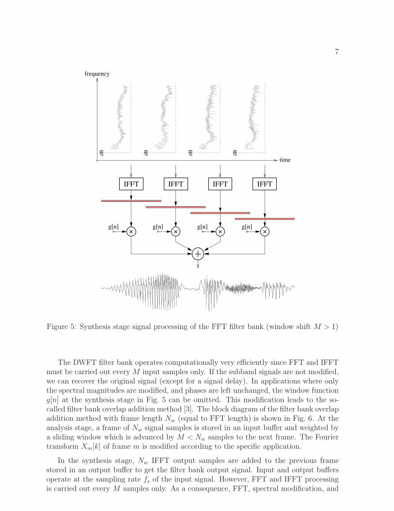
Figure 5: Synthesis stage signal processing of the FFT filter bank (window shift M > 1)

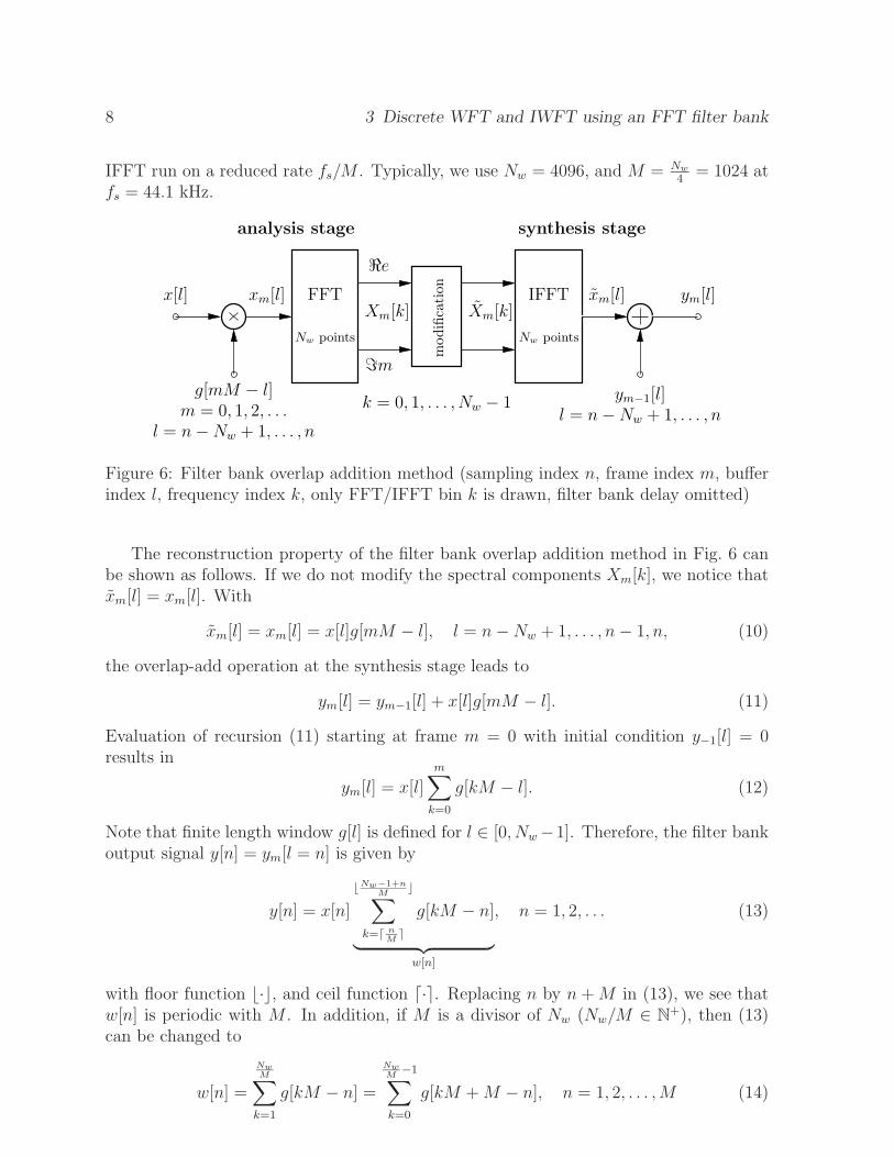
The DWFT filter bank operates computationally very efficiently since FFT and IFFTmust be carried out every M input samples only. If the subband signals are not modified,we can recover the original signal (except for a signal delay). In applications where onlythe spectral magnitudes are modified, and phases are left unchanged, the window functiong[n] at the synthesis stage in Fig. 5 can be omitted. This modification leads to the so-called filter bank overlap addition method [3]. The block diagram of the filter bank overlapaddition method with frame length Nw (equal to FFT length) is shown in Fig. 6. At theanalysis stage, a frame of Nw signal samples is stored in an input buffer and weighted bya sliding window which is advanced by M < Nw samples to the next frame. The Fouriertransform Xm[k] of frame m is modified according to the specific application.

In the synthesis stage, Nw IFFT output samples are added to the previous framestored in an output buffer to get the filter bank output signal. Input and output buffersoperate at the sampling rate fs of the input signal. However, FFT and IFFT processingis carried out every M samples only. As a consequence, FFT, spectral modification, and


IFFT run on a reduced rate fs/M . Typically, we use Nw = 4096, and M = Nw

4= 1024 at

fs = 44.1 kHz.

FFT IFFTx[l] xm[l]

Nw points Nw points

ym[l]

g[mM − l] ym−1[l]

Xm[k]

l = n−Nw + 1, . . . , nl = n−Nw + 1, . . . , n

ℑm

k = 0, 1, . . . , Nw − 1

Xm[k]

m = 0, 1, 2, . . .

ℜexm[l]

analysis stage synthesis stage

modification

Figure 6: Filter bank overlap addition method (sampling index n, frame index m, bufferindex l, frequency index k, only FFT/IFFT bin k is drawn, filter bank delay omitted)

The reconstruction property of the filter bank overlap addition method in Fig. 6 canbe shown as follows. If we do not modify the spectral components Xm[k], we notice thatxm[l] = xm[l]. With

xm[l] = xm[l] = x[l]g[mM − l], l = n−Nw + 1, . . . , n− 1, n, (10)

the overlap-add operation at the synthesis stage leads to

ym[l] = ym−1[l] + x[l]g[mM − l]. (11)

Evaluation of recursion (11) starting at frame m = 0 with initial condition y−1[l] = 0results in

ym[l] = x[l]m∑

k=0

g[kM − l]. (12)

Note that finite length window g[l] is defined for l ∈ [0, Nw−1]. Therefore, the filter bankoutput signal y[n] = ym[l = n] is given by

y[n] = x[n]

⌊Nw−1+n

M⌋

∑

k=⌈ n

M⌉

g[kM − n]

︸︷︷︸

w[n]

, n = 1, 2, . . . (13)

with floor function ⌊·⌋, and ceil function ⌈·⌉. Replacing n by n +M in (13), we see thatw[n] is periodic with M . In addition, if M is a divisor of Nw (Nw/M ∈ N

+), then (13)can be changed to

w[n] =

Nw

M∑

k=1

g[kM − n] =

Nw

M−1

∑

k=0

g[kM +M − n], n = 1, 2, . . . ,M (14)

9

because ⌈ nM⌉ = 1, ⌊Nw−1+n

M⌋ = Nw

Mfor n ∈ [1,M ]. We get perfect reconstruction if

w[n] = 1,∀n. It will be shown that w[n] = aNw

Mfor the window functions given below.

As an example, the reconstruction error for M ∈ [1, Nw

2] and Nw = 200 is displayed in

Fig. 7. For M < Nw

4, the observed error is in [−10−3, 10−3], and is negligible for all

practical applications. Perfect reconstruction is achieved if Nw/M ∈ N+ and by selecting

10 20 30 40 50 60 70 80 90 100

10−15

10−10

10−5

100

window shift M

ma

x(|

e[n

]|)

max. reconstruction error, window length = 200

Figure 7: Overlap-add FFT filter bank reconstruction error e[n] = y[n]−x[n] as a functionof window shift M (Nw = 200, perfect reconstruction for Nw/M ∈ N

+).

the cosine-type windows

g[n] =

a− b cos

(π

Nw

(2n+ 1)

)

0 ≤ n ≤ Nw − 1

0 else

(15)

with a = b = 0.5, or a = 0.54, b = 0.46. Inserting g[n] of (15) as g[n] in (14) and usingthe sum formula of a finite geometric series gives

w[n] = aNw

M− bℜe

ejπ

Nw(2M−2n+1)

Nw

M−1

∑

k=0

ejπ

NwMk

︸︷︷︸

0

= aNw

M. (16)

Thus, we have proved that the window function of (15) indeed ensures perfect reconstruc-tion. According to (16), g[n] must be normalized:

g[n] =M

aNw

g[n] . (17)

It should be noted that MATLABr functions hanning(), hann(), and hamming() usedifferent window definitions, and do not deliver perfect reconstruction for N/M ∈ N

+.

A MATLABr code segment of the filter bank overlap addition method without spectralmodification can be written as follows:

10 4 Perfect reconstruction overlap-add FFT-Filter banks with fractional oversampling

N = 512; % signal length

Nw = 128; % window length

M = 32; % frame hop size (a divisor of Nw)

n = 0:N-1;

x = sin(2*pi*0.02*n); % input signal

g = 0.5*(1-cos(pi/Nw*(2*(0:Nw-1)+1))); % time window function g[n]

g = M/(0.5*Nw)*g; % normalize g[n]

y = zeros(1,N); % output signal vector

Nf = Nw; % FFT length = Nw

for m = 1:M:N-Nw+1 % frame processing loop, M = frame hop size

% analysis stage (apply weighting function and FFT to frame)

m1 = m:m+Nw-1; % indices of current frame

X = fft(x(m1).*g,Nf);

% synthesis stage (overlap-add of successive IFFT outputs)

y(m1) = y(m1) + real(ifft(X,Nf));

end

The perfect reconstruction property of the IDWFT (Fig. 5) can be proved similar tothe overlap-addition filter bank. Since we need a window function in the overlap-addoperation (see (9)), requirement (14) is modified to

w[n] =

Nw

M−1

∑

k=0

g2[kM +M − n], n = 1, 2, . . . ,M . (18)

With cosine-window (15), we get after some intermediate steps

w[n] =

(

a2 +b2

2

)Nw

M. (19)

Thus, the IDWFT needs a window normalization factor√M√

Nw(a2+b2/2)for each of the two

windows of the DWFT/IDWFT filter bank.

4 Perfect reconstruction overlap-add FFT-Filter banks

with fractional oversampling

Perfect reconstruction of the Nw-point FFT filter bank presented in the previous sectionis possible for special window shifts M only (Nw/M ∈ N

+). In addition, the time windowis restricted to a raised cosine function. Flexibility in choosing oversampling factors, andspectral selectivity is thus limited. In this section, we show that by a proper design of the

4.1 Frame-based design of overlap-add FFT filter banks with fractional oversampling11

synthesis window function perfect reconstruction can be achieved for all window shifts1 ≤ M < Nw, and for different kinds of window functions. In addition, we get a closedform solution. The design is based on the theory of frames [1].

Frames can be thought as a generalization of bases in a vector space. Normally,an orthogonal basis is used to represent or approximate signals as vectors in a functionspace. An example is the Fourier transform. However, we can also select basis vectors{φn : n ∈ Γ} which are neither orthogonal, nor even linearly independent to representsignals by linear combinations of these vectors (Γ is a finite or infinite set of indices).1

The signal representation f =∑

n∈Γ 〈f, φn〉︸︷︷︸

cn

φn is stable, if the expansion coefficients cn

obey

A ‖f‖2 ≤∑

n∈Γ|〈f, φn〉|2︸︷︷︸

|cn|2

≤ B ‖f‖2 , (20)

where 〈., .〉 is the vector inner product, and A,B are the frame bounds (0 < A ≤ B).Relationship (20) is a generalization of Parseval’s equation ‖f‖2 =

∑

n∈Γ |cn|2 which is

valid for orthonormal bases. If A = B then we have a tight frame. An orthonormal basisis a tight frame with A = B = 1. If B ≫ A, then the signal representation is unstable,i.e. it is very sensitive to errors of expansion coefficients cn. A frame is called a Rieszbasis, if the basis vectors {φn : n ∈ Γ} are linearly independent.

The main problem to analyze and reconstruct signals with frames is to find a frameoperator Φ and the associated inverse operator Φ:

cn = Φf = 〈f, φn〉, f = Φ c =∑

n∈Γcnφn . (21)

In case of discrete-time signals, Φ is a matrix, and Φ may be calculated with the pseudoinverse Φ+ = (ΦHΦ)−1ΦH . In the following, we show how Φ can be derived for theanalysis stage of the FFT filter bank, and how Φ+ of the synthesis stage can be computedwithout matrix inversion. To avoid boundary effects (settling periods), we take f as aninfinite-length, discrete-time signal x[n], n ∈ Z.

4.1 Frame-based design of overlap-add FFT filter banks with

fractional oversampling

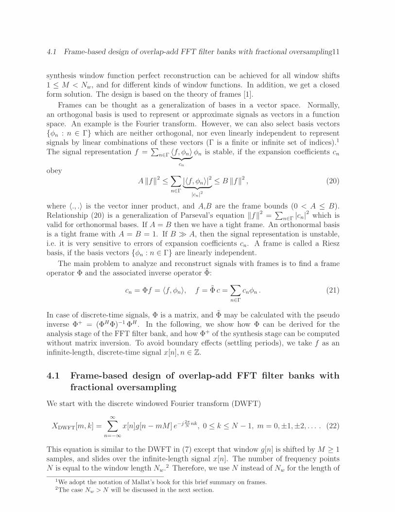
We start with the discrete windowed Fourier transform (DWFT)

XDWFT[m, k] =∞∑

n=−∞x[n]g[n −mM ] e−j 2π

Nnk, 0 ≤ k ≤ N − 1, m = 0,±1,±2, . . . . (22)

This equation is similar to the DWFT in (7) except that window g[n] is shifted by M ≥ 1samples, and slides over the infinite-length signal x[n]. The number of frequency pointsN is equal to the window length Nw.

2 Therefore, we use N instead of Nw for the length of

1We adopt the notation of Mallat’s book for this brief summary on frames.2The case Nw > N will be discussed in the next section.


window g[n], n ∈ [0, N−1]. Due to the finite duration of g[n], (n−mM) can be restrictedto [0, N − 1]. Thus, summation index n is needed only in [mM,N − 1 + mM ],m =0,±1,±2, . . ., and (22) can be rewritten as follows:

XDWFT[m, k] =N−1+mM∑

n=mM

x[n]g[n−mM ] e−j 2π

Nnk

=N−1∑

n=0

x[n+mM ]g[n] e−j 2π

Nnke−j 2π

NmM

= e−j 2π

NmM

N−1∑

n=0


Nnk , 0 ≤ k ≤ N − 1, m = 0,±1,±2, . . . .

(23)

According to (23), we shift a signal block into the window support [0, N−1] at everyM -thsample, multiply the block samples with the window function g[n], and apply the N -pointDFT to get the DWFT at window position mM . The linear phase factor compensatesthe signal shift by mM samples. With Cm,k = XDWFT[m, k]ej

2π

NmM , Wk,n = e−j 2π

Nnk, and

gn = g[n], the filter bank analysis stage operation is

Cm,k =N−1∑

n=0

gnWk,n x[n+mM ] , 0 ≤ k ≤ N − 1, m = 0,±1,±2, . . . . (24)

Cm,k in (24) are the coefficients of a frame-based signal analysis as given in (21). At firstglance, it is not obvious how to find the frame operator since x[n] in (24) is choppedinto overlapping blocks of N samples. However, the following matrix and vector formof (24), and a graphical illustration of the matrix structure leads to the solution. Wecollect coefficients Cm,k to vectors cm = (Cm,0, . . . , Cm,N−1)

T , and signal blocks to vectorsxm = (x[mM ], . . . , x[N − 1 +mM ])T , respectively. Equation (24) can now be written invector form as

cm = Φaxm , m = 0,±1,±2, . . . (25)

with N ×N matrix

Φa =

g0W0,0 g1W0,1 . . . gN−1W0,N−1

g0W1,0 g1W1,1 . . . gN−1W1,N−1

. . . . . . . . . . . . . . . . . . . . . . . . . . . . . .

g0WN−1,0 g1WN−1,1 . . . gN−1WN−1,N−1

. (26)

The frame matrix (operator) Φ is unveiled by stacking all coefficient vectors cm toan infinite-length column vector as shown in Fig. 8. We get vectors and a matrix withinfinite dimension since the input signal has infinite duration. The block overlapping isobtained by shifting Φa by M indices for each signal block. Note that frame matrix Φ isnot a square matrix.3 As a consequence, the pseudo inverse Φ+ is needed to reconstruct

3If we consider a finite-length segment of x, then we get a rectangular matrix Φ.


c0

c1

c2

Φa

Φa

Φa

0

0

N

N

N

=

c = Φ x

N

N

M

x1

N

N

N

x0

x2

M

Figure 8: Frame operator (matrix) Φ of filter bank analysis stage c = Φx

signal x from coefficients c. Although Φ has infinite dimension, the special structureof Φ ensures that multiplications and additions give bounded results when computinge.g. ΦHΦ in Φ+ = (ΦHΦ)−1ΦH . Furthermore, we will show that ΦHΦ is a diagonalmatrix.

Φa

Φa

Φa

N

0

0 0

0

M

Φd S

1

1

1

=Φ

Figure 9: Factorization of Φ in block-diagonal matrix Φd and matrix S of shifted identitymatrices

We start with a factorization of Φ in a block-diagonal matrix Φd, and a shifting matrixS as illustrated in Fig. 9. Note that STS is a diagonal matrix. Using Φ = ΦdS inΦHΦ, weget ΦHΦ = STΦH

d ΦdS. Inspecting the columns of Φa in (26), we notice that the columnsare orthogonal because Φa is basically a DFT matrix with column elements modified bythe same factor gi. Thus we get a diagonal matrix ΦH

a Φa = N diag(g20, g21 , . . . , g

2N−1). As


a consequence, ΦHd Φd is a diagonal matrix with a diagonal obtained by repetitions of the

diagonal of ΦHa Φa:

ΦHa Φa = Da Da(i, j) =

{

Ng2i i = j

0 i 6= j, i, j = 0, 1, . . . N − 1 (27)

ΦHd Φd = Dd Dd(i, j) = Da(i⊕N, j ⊕N) , i, j = 0,±1,±2, . . . (28)

(⊕ is the modulo operation for positive and negative numbers).

To compute ΦHΦ = STΦHd ΦdS = STDdS, we first observe that DdS has a shift

structure too, where the ones in the shifted diagonals of S are replaced by the diagonalelements (27) of Da. Next, we inspect the multiplication of ST with DdS in Fig. 10.Performing the matrix multiplication in Fig. 10, we get a diagonal matrixD with elements

ST

0

0

M

0

0

M

DdS

d

d

d

1

1

1

N

Figure 10: Computation of ΦHΦ = STDdS (d is the vector of diagonal elements of (27))

computed with ⌈NM⌉ and ⌈N

M⌉−1 overlapping diagonals. As a result, the diagonal elements

D(i, i) are obtained by

ΦHΦ = D , D(i, i) =

N

⌈ N

M⌉−1

∑

m=0

g2i+mM 0 ≤ i ≤ M1 − 1

N

⌈ N

M⌉−2

∑

m=0

g2i+mM M1 ≤ i ≤ M − 1

, (29)

with M1 = M +N −⌈NM⌉M . In addition, D(i, i) is periodic with M . Therefore, D(i, i) is

periodically extended for all i. This findings are illustrated in Fig. 11 where the hatchedrectangles indicate the regions that contribute to the diagonal ofΦHΦ. M1, M2 determinethe indices i of the elements on the diagonals of ΦH as given in (29). We notice thatthe pseudo inverse of the frame matrix Φ can now be computed efficiently since matrix


��

��

N

M2 = ⌈NM⌉M −N

M1 = N +M − ⌈NM⌉M

M

Figure 11: Regions of ST that contribute to diagonal of ΦHΦ = STDdS (N/M = 3, M1,M2 are the heights of the hatched rectangles)

inversion is reduced to scalar divisions:

Φ+ = (ΦHΦ)−1ΦH = DsΦH (30)

Ds(i, j) =

{1

D(i⊕M,i⊕M)i = j

0 i 6= ji, j = 0,±1,¸± 2, . . . (31)

with D(i, i) of (29), and modulo operation ⊕. The filter bank synthesis stage with theinverse frame operator Φ+ is sketched in Fig. 12 (with Φ shown in Fig. 8).

M

y2

y1+

+

y =

=

N

N

N

y0

Ds0ΦHaN

N

Ds0ΦHa

Ds0ΦHa

0

0

Φ+

M

c

c0

c1

c2

N

N

N

Figure 12: Inverse frame operator of filter bank synthesis stage y = Φ+c (Ds0 has elementsDs(i, j), i, j = 0, 1, . . . , N − 1)

Each output signal block ym is computed with the corresponding filter bank analysiscoefficients cm and Ds0Φ

Ha of Φ+ (Ds0 is the sub-matrix of Ds using element indices


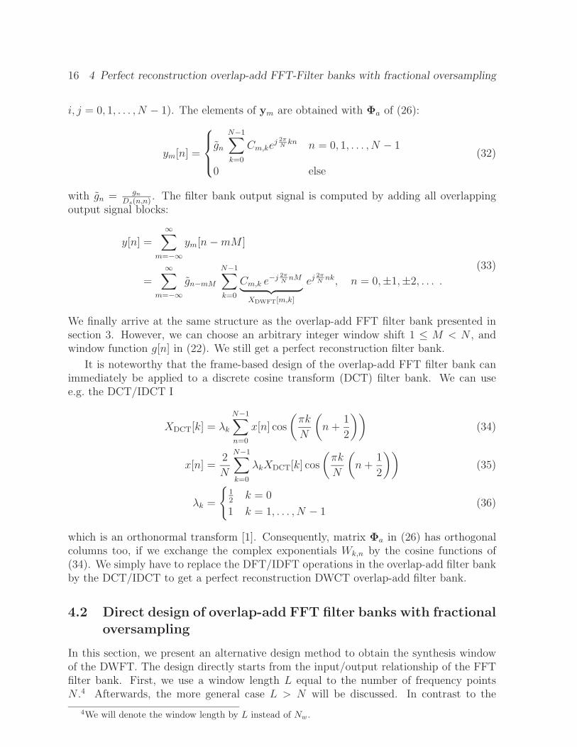
i, j = 0, 1, . . . , N − 1). The elements of ym are obtained with Φa of (26):

ym[n] =

gn

N−1∑

k=0

Cm,kej 2π

Nkn n = 0, 1, . . . , N − 1

0 else

(32)

with gn = gnDs(n,n)

. The filter bank output signal is computed by adding all overlappingoutput signal blocks:

y[n] =∞∑

m=−∞ym[n−mM ]

=∞∑

m=−∞gn−mM

N−1∑

k=0

Cm,k e−j 2π

NnM

︸︷︷︸

XDWFT[m,k]

ej2π

Nnk, n = 0,±1,±2, . . . .

(33)

We finally arrive at the same structure as the overlap-add FFT filter bank presented insection 3. However, we can choose an arbitrary integer window shift 1 ≤ M < N , andwindow function g[n] in (22). We still get a perfect reconstruction filter bank.

It is noteworthy that the frame-based design of the overlap-add FFT filter bank canimmediately be applied to a discrete cosine transform (DCT) filter bank. We can usee.g. the DCT/IDCT I

XDCT[k] = λk

N−1∑

n=0

x[n] cos

(πk

N

(

n+1

2

))

(34)

x[n] =2

N

N−1∑

k=0

λkXDCT[k] cos

(πk

N

(

n+1

2

))

(35)

λk =

{12

k = 0

1 k = 1, . . . , N − 1(36)

which is an orthonormal transform [1]. Consequently, matrix Φa in (26) has orthogonalcolumns too, if we exchange the complex exponentials Wk,n by the cosine functions of(34). We simply have to replace the DFT/IDFT operations in the overlap-add filter bankby the DCT/IDCT to get a perfect reconstruction DWCT overlap-add filter bank.

4.2 Direct design of overlap-add FFT filter banks with fractional

oversampling

In this section, we present an alternative design method to obtain the synthesis windowof the DWFT. The design directly starts from the input/output relationship of the FFTfilter bank. First, we use a window length L equal to the number of frequency pointsN .4 Afterwards, the more general case L > N will be discussed. In contrast to the

4We will denote the window length by L instead of Nw.

4.2 Direct design of overlap-add FFT filter banks with fractional oversampling 17

frame-based approach of the previous section, we need a matrix inversion. Our design isusing a given analysis window, and determines the corresponding synthesis window whichensures perfect signal synthesis (reconstruction). This approach is different to the Gaborexpansion (transform) where the synthesis window is given, and the analysis window hasto be found [5]. By interchanging analysis and synthesis window, however, we can easilyinclude the Gabor transform in our design program.

Combining (22) of the analysis part of the overlap-add FFT filter bank with (33) leadsto the following input/output relationship:

y[n] =∞∑

m=−∞

∞∑

n′=−∞x[n′] gn−mM gn′−mM

N−1∑

k=0

ej2π

Nk(n−n′)

︸︷︷︸

N if n−n′=lN, 0 otherwise

=∞∑

m=−∞

∞∑

n′=−∞x[n′] gn−mM gn′−mMN δ[n− n′ − lN ]

= x[n− lN ]N∞∑

m=−∞gn−mM gn−mM−lN , l = 0,±1,±2, . . .

(37)

(δ[·] is the unit impulse). For the case L = N , the finite length analysis window gn withn ∈ [0, N − 1] requires n−mM ∈ [0, N − 1]. Therefore, we only need l = 0 in (37) to getwith −m → m the constraints

⌊N−1−n

M⌋

∑

m=0

gn+mM gn+mM =1

N, n = 0, . . .M − 1 (38)

to guarantee perfect reconstruction of the input signal. The constraints (38) are usedto find the synthesis window gn, n ∈ [0, N − 1]. With matrix notation, we obtain thefollowing underdetermined set of linear equations:

Gg =1

N1M . (39)

1M is the M × 1 vector with 1 elements, and g = (g0, g1, . . . , gN−1)T contains the wanted

synthesis window. M ×N matrix G has non-zero elements at indices (i, j) = (i, i+ jM)only:

G(i, i+ jM) = gi+jM , i = 0, . . . ,M − 1, j = 0, . . . ,

⌊N − 1− i

M

⌋

. (40)

An obvious solution of (39) with the pseudo-inverse G+ of G is

g =1

NG+ 1M . (41)

Note that the multiplication by 1M in (41) can be removed by summing up the elementsof each row of G+.

We now discuss the case L > N which offers more flexibility in choosing the windowlength L. It should be noted, however, that the frame hop size M , and the number of


frequency points N determine the paritioning of the time-frequency plane, and must obeythe uncertainity principle to ensure a stable signal reconstruction. We assume that L isa multiple of N . The signal can have any length greater or equal to L.

For L > N we need to consider l = 0,±1,±2, . . . in (37) to get

⌊L−1−n−lN

M⌋

∑

m=0

gn+mM gn+mM+lN =1

Nδ[l] , l = 0,±1,±2, . . . ,±

⌊L− 1

N

⌋

. (42)

The selection of index n depends on l. Taking the window support [0, L−1] into account,and inspecting the index n+mM + lN in (42) leads to

n =

{

0, 1, 2, . . . ,M − 1 l ≥ 0

−lN,−lN + 1, . . .− lN +M − 1 l < 0. (43)

We now get an augmented set of linear equations in the following matrix form:

Gg =1

Nv . (44)

Matrix G in (44) has size 2M LN×L, and non-zero elements G(lM+i, i+jM) = gi+jM+lN ,

and G(lM +M + i, i+ jM+ lN) = gi+jM , with i = 0, 1, . . . ,M −1, j = 0, 1, . . . , ⌊(L−1−i− lN)/M⌋, l = 0, 1, . . . ⌊(L− 1)/N⌋. Vector v contains M ones followed by 2M L

N−M

zeros.

For L > N , we must modify the analysis part (23) since the windowed signal haslength L but the DFT is computed at N frequency points only:

XDWFT[m, k] = e−j 2π

NmM

L−1∑

n=0


Nnk

= e−j 2π

NmM

L

N−1

∑

l=0

N−1∑

n′=0

x[n′ + lN +mM ]g[n′ + lN ] e−j 2π

N(n′+lN)k

︸︷︷︸

N-point DFT

.(45)

(Note that L is a multiple of N , and k = 0, 1, . . . , N − 1.) The synthesis part must bemodified too because the inverse DFT in (32) delivers an N -point signal which has to bemultiplied with the synthesis window of length L. The simple solution is to periodicallyextend the inverse DFT result to obtain a signal of length L. This signal can then bemultiplied with the synthesis window.

We have implemented this design method in MATLABr programs dwft1.m, anddwft2.m (Gabor transform). As already discussed on page 16, we can extend the directdesign of the overlap-add FFT filter bank to the weighted DCT filter bank by replacingthe DFT by the DCT given in (34).

4.3 Design examples 19

4.3 Design examples

We conclude this section with some experimental results using our MATLABr programwft_frames.m for the frame-based design method. The programs dwft1.m, and dwft2.m

(Gabor transform) implement the direct design method to be used for L ≥ N . The WCTdesign programs are wct_frames.m, dwct1.m, and dwct2.m, respectively. The selectedwindow type is a Gaussian function. Other windows like raised cosine, or an FIR lowpass filter impulse response are alternative selections in our programs. Test signal isa sinusoidal chip. All design examples exhibit a perfect reconstruction property withinmachine precision.5

A frame-based WFT design example is shown in Fig. 13 to Fig. 15.

0 50 100 150 200 250 300 350 400 450 500

n

-1

-0.5

0

0.5

1

x[n

]

input signal

WFT magnitude, Nw

= 64, M = 7, oversampling = 9.1429

0 50 100 150 200 250 300 350 400 450

n

0

0.1

0.2

0.3

0.4

0.5

f/f s

1

2

3

4

5

6

7

Figure 13: DWFT of sinusoidal chirp (Gaussian analysis window, frame-based design)

The frame bounds are very close indicating that the basis functions form a nearlytight frame. The tight frame bounds are lost, if the window shift M is to large to ensurea dense coverage of the time-frequency plane. Our experiments show that a cosine typewindow performs much better (closer frame bounds) in case of large window shifts. FIRfilter windows exhibit the worst result regarding the frame bounds. In general, M shouldbe less than N/2 to get a filter bank oversampling greater than 2. Nevertheless we achievea perfect reconstruction, even if we would choose M > N/2.

5The error plots have a reduced time interval because the overlap-add filter bank settling periods at

signal begin and end are removed. Consequently, we get the same results as with infinite-duration signals.


0 10 20 30 40 50 60 70

n

0

0.2

0.4

0.6

0.8

g[n

]gaussian analysis window, 2 = 1.00

0 10 20 30 40 50 60 70

n

0

0.2

0.4

0.6

0.8

gs[n

]

synthesis window, frame bounds A = 9.1428, B = 9.1430

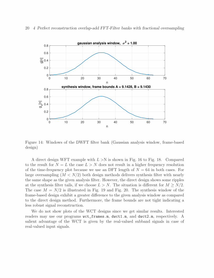
Figure 14: Windows of the DWFT filter bank (Gaussian analysis window, frame-baseddesign)

A direct design WFT example with L >N is shown in Fig. 16 to Fig. 18. Comparedto the result for N = L the case L > N does not result in a higher frequency resolutionof the time-frequency plot because we use an DFT length of N = 64 in both cases. Forlarge oversampling (M < N/2) both design methods delivers synthesis filter with nearlythe same shape as the given analysis filter. However, the direct design shows some ripplesat the synthesis filter tails, if we choose L > N . The situation is different for M ≥ N/2.The case M = N/2 is illustrated in Fig. 19 and Fig. 20. The synthesis window of theframe-based design exhibit a greater difference to the given analysis window as comparedto the direct design method. Furthermore, the frame bounds are not tight indicating aless robust signal reconstruction.

We do not show plots of the WCT designs since we get similar results. Interestedreaders may use our programs wct_frames.m, dwct1.m, and dwct2.m, respectively. Asalient advantage of the WCT is given by the real-valued subband signals in case ofreal-valued input signals.


50 100 150 200 250 300 350 400 450

n

-5

-4

-3

-2

-1

0

1

2

3

4

e[n

]10

-16 reconstruction error, max(|e[n]|) = 4.441e-16

Figure 15: Reconstruction error of the DWFT filter bank (Gaussian analysis window,frame-based design)

0 50 100 150 200 250 300 350 400 450 500

n

-1

-0.5

0

0.5

1

x[n

]

input signal

WFT magnitude, N = 64, M = 7, L = 128, oversampling = 9.1429

0 50 100 150 200 250 300 350 400 450

n

0

0.1

0.2

0.3

0.4

0.5

f/f s

1

2

3

4

5

6

Figure 16: DWFT of sinusoidal chirp (Gaussian analysis window, direct design method)


0 20 40 60 80 100 120 140

n

0

0.2

0.4

0.6

g[n

]

gaussian analysis window, 2 = 1.00

0 20 40 60 80 100 120 140

n

-0.2

0

0.2

0.4

0.6

gs[n

]

synthesis window (direct design method)

Figure 17: Windows of the DWFT filter bank (Gaussian analysis window, direct designmethod)

100 150 200 250 300 350 400

n

-3

-2

-1

0

1

2

3

e[n

]

10-15 reconstruction error, max(|e[n]|) = 2.776e-15

Figure 18: Reconstruction error of the DWFT filter bank (Gaussian analysis window,direct design method)


0 10 20 30 40 50 60 70

n

0

0.5

1

1.5

g[n

]gaussian analysis window, 2 = 1.00

0 10 20 30 40 50 60 70

n

0

0.5

1

1.5

gs[n

]

synthesis window, frame bounds A = 0.6801, B = 3.4316

Figure 19: Windows of the DWFT filter bank (Gaussian analysis window, frame-baseddesign method, N = 64, M = N/2 = 32)

0 20 40 60 80 100 120 140

n

0

0.5

1

g[n

]

gaussian analysis window, 2 = 1.00

0 20 40 60 80 100 120 140

n

-0.5

0

0.5

1

gs[n

]

synthesis window (direct design method)

Figure 20: Windows of the DWFT filter bank (Gaussian analysis window, direct designmethod, N = 64, M = N/2 = 32, L = 128)

24 5 Uniform DFT filter banks with fractional oversampling

5 Uniform DFT filter banks with fractional oversam-

pling

The overlap-add FFT filter banks presented in the previous section are typically designedwith window lengths equal or twice the FFT length (i.e. the number of filter bank channelsin [0, fs]). In addition, the commonly used analysis windows do not provide a high selec-tivity of the channel transfer functions. Uniform DFT filter banks (and cosine-modulatedfilter banks) offer much more flexibility in choosing the filter length, and the number offilter bank channels. In this section, we discuss filter bank designs based on frame theory,and on paraunitarity [2, 8]. With the first design method, we select the analysis filters,and compute the respective synthesis filters similar to the WFT frame-based design. Inthe second approach, both the analysis filters and the synthesis filters are obtained by anoptimization procedure which ensures perfect input signal reconstruction combined witha high filter selectivity.

The N channels of a uniform DFT filter bank are created by modulating a prototypefilter by complex exponentials. As shown in Fig. 21, the channels can be odd-stackedor even-stacked along the frequency axis (θ ∈ [0, 2π]). Odd-stacked filters have center

H1 H2 H3 H4 HN−1

H0 H1 H2 H3 H4 HN−1

H0

0 π 2π

0 π 2π

π

N

2π

N

θ3π

N

4π

N

θ

Figure 21: Filter stacking of N = 6 channel DFT filter bank for frequencies θ ∈ [0, 2π],odd-stacked ideal filters (above), even-stacked ideal filters (below)

frequencies that are odd multiples of πN. The center frequencies of even-stacked filters

start at zero, and are even multiples of πN.

The block diagram Fig. 22 shows an N -channel analysis/synthesis filter bank withdecimation factorM . Oversampled filter banks use 1 ≤ M < N resulting in more subbandsamples per unit time as samples of the input (or output) signal. Thus, the set of subbandsignals are the expansion coefficients of a redundant signal representation similar to theoverlap-add FFT filter bank. The subband signals in Fig. 22 are the down-sampled filteroutput signals

vk[n] =∞∑

m=−∞x[m]hk[nM −m] = 〈x, hk,n〉, k = 0, 1, . . . , N − 1, (46)

25

hN−1[n] ↓M ↑M fN−1[n]vN−1[n]

h1[n] ↓M ↑M f1[n]v1[n]

h0[n] ↓M ↑M f0[n]v0[n]x[n]

y[n]

Figure 22: Block diagram of an N -channel analysis/synthesis filter bank (integer over-sampling for N divisible by M , fractional oversampling otherwise)

with hk,n[m] = h∗k[nM −m].

At the synthesis stage, up-sampling, filtering, and summation results in the outputsignal

y[n] =N−1∑

k=0

∞∑

m=−∞vk[m] fk[n−mM ] =

N−1∑

k=0

∞∑

m=−∞〈x, hk,m〉fk,m[n], (47)

with fk,m[n] = fk[n − mM ]. Therefore, the filter bank operation is a signal expansionwith a basis function set {fk,m[n] : k = 0, 1, . . . , N − 1, m = 0,±1,±2, . . .}. If thereconstruction of the filter bank system is perfect, then we get y[n] = x[n],∀n.6

In principle, we can use (47) to get the frame operator, and it’s inverse as given in(21). Finding the inverse operator, however, is not as easy as in case of the overlap-addFFT filter bank. The time-domain frame operator of filter banks is an infinite-dimensionalmatrix with a structure similar to matrix Φ in Fig. 8. The important difference, however,is that sub-matrix Φa is not square but has dimension N × L where L is the (FIR) filterlength of hk[n].

To illustrate the structure of the analysis frame matrix Φ we consider a DFT-filterbank with N = 10 channels, and an analysis FIR filter length L = 20. In case of integeroversampling (N/M ∈ N

+) and N even, the analysis frame matrix Φ, and the matricesinvolved in the computation of the pseudo inverse Φ+ = (ΦHΦ)−1ΦH are shown inFig. 23. Note that only parts of the infinite-dimensional matrices are plotted. Similar toFig. 8, the image of Φ shows N × L blocks shifted by M indices. These blocks representthe N FIR filters of the analysis stage. The image of the pseudo inverse indicates thatthe synthesis frame operator is just the conjugate transpose of Φ scaled by the constantdiagonal elements of (ΦHΦ)−1.

The situation is quite different when N is not divisible by M (fractional oversam-pling). The images in Fig. 24 show the presence of weak side diagonals in (ΦHΦ), andin (ΦHΦ)−1, respectively. As a consequence, the synthesis filter impulse responses have alonger duration than the analysis filters. Similar results are obtained with N odd (even in

6We omit the signal delay in case of causal filters. The filter bank delay will be included later on.


the case of integer oversampling). The author’s MATLABr program dftfib_inverse.m

can be used to investigate all interesting cases.

magnitude of Φ

5 10 15 20 25 30 35

j

20

40

60

80

100

120

i

(Φ' Φ)

5 10 15 20 25 30 35

j

5

10

15

20

25

30

35

i

(Φ' Φ)-1

5 10 15 20 25 30 35

j

5

10

15

20

25

30

35

i

magnitude of Φ+ = (Φ' Φ)

-1 Φ'

20 40 60 80 100 120

j

5

10

15

20

25

30

35

i

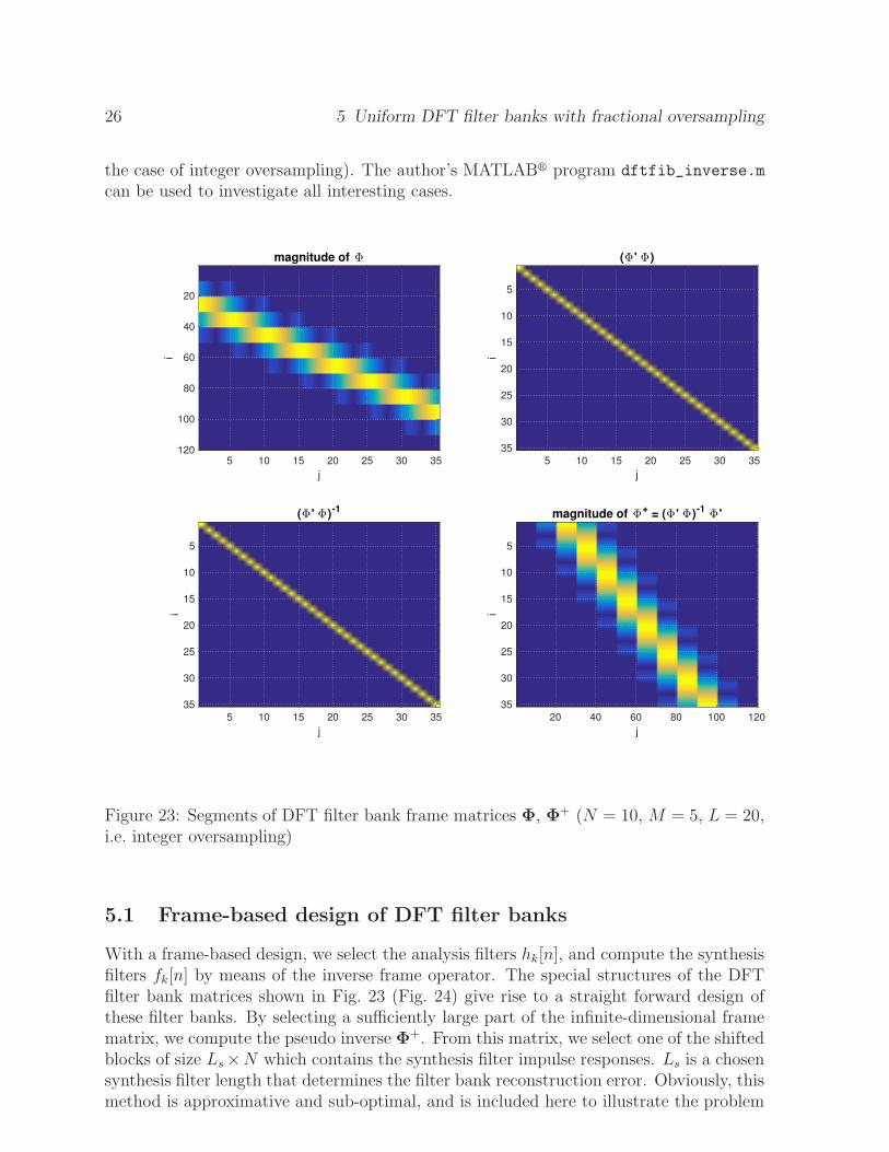
Figure 23: Segments of DFT filter bank frame matrices Φ, Φ+ (N = 10, M = 5, L = 20,i.e. integer oversampling)

5.1 Frame-based design of DFT filter banks

With a frame-based design, we select the analysis filters hk[n], and compute the synthesisfilters fk[n] by means of the inverse frame operator. The special structures of the DFTfilter bank matrices shown in Fig. 23 (Fig. 24) give rise to a straight forward design ofthese filter banks. By selecting a sufficiently large part of the infinite-dimensional framematrix, we compute the pseudo inverse Φ+. From this matrix, we select one of the shiftedblocks of size Ls×N which contains the synthesis filter impulse responses. Ls is a chosensynthesis filter length that determines the filter bank reconstruction error. Obviously, thismethod is approximative and sub-optimal, and is included here to illustrate the problem

5.1 Frame-based design of DFT filter banks 27

magnitude of Φ

5 10 15 20 25 30 35

j

20

40

60

80

100

120

140

160

i

(Φ' Φ)

5 10 15 20 25 30 35

j

5

10

15

20

25

30

35

i

(Φ' Φ)-1

5 10 15 20 25 30 35

j

5

10

15

20

25

30

35

i

magnitude of Φ+ = (Φ' Φ)

-1 Φ'

50 100 150

j

5

10

15

20

25

30

35

i

Figure 24: Segments of DFT filter bank frame matrices Φ, Φ+ (N = 10, M = 4, L = 20,i.e. fractional oversampling)

of finding the inverse of an infinite-dimensional frame matrix. As shown in [2], infinite-dimensional frame matrices can be avoided by a polyphase decomposition. However, wenow get an infinite set of finite-dimensional frame matrices in the z-domain. Therefore,we have to compute this set at discrete frequencies. In general, this is leading us toapproximate filter design solutions too.

To obtain the frame operator, we use the finite length analysis filters

hk[n] =

{

g[n] ejπ

N(2k+1)(n−Nd) odd-stacked filters

g[n] ej2π

Nk(n−Nd) even-stacked filters

, k = 0, 1, . . . , N − 1 (48)

where g[n] ∈ [0, L− 1] is a real-valued lowpass prototype impulse response, and Nd is thefilter delay. Inserting hk[n] of (48) in (46) and observing nM −m ∈ [0, L− 1] yields

vk[n] =nM−L+1∑

m=nM

x[m]hk[nM −m] =L−1∑

m=0

hk[m]x[nM −m], k = 0, 1, . . . , N − 1. (49)


The frame matrix can be found by the steps used with the overlap-add FFT filter bankon page 12. Defining the subband signal vector vn = (v0[n], . . . , vN−1[n])

T , and signalblock xn = (x[nM ], . . . , x[nM − L+ 1])T , we obtain from (49)

vn = Φaxn, n = 0,±1,±2, . . . (50)

where the N × L matrix collects the channel filter impulse responses as rows:

Φa =

g0W0,0 g1W0,1 . . . gL−1W0,L−1

g0W1,0 g1W1,1 . . . gL−1W1,L−1

. . . . . . . . . . . . . . . . . . . . . . . . . . . . .

g0WN−1,0 g1WN−1,1 . . . gL−1WN−1,L−1

. (51)

We use gn = g[n], and Wk,n denoting the exponential factors as given in (48). Stackingsubband signal vectors vn to an infinite-length column vector results in a frame matrixΦ with sub-matrices Φa shifted by M indices as illustrated by the upper left image inFig. 23.

As opposed to the frame matrix in Fig. 8, however, we now get N × L sub-matricesinstead of N × N matrices. Consequently, ΦH

a Φa is not diagonal but shows symmetricside diagonals. Thus, we cannot derive the pseudo inverse Φ+ in closed form as in caseof the overlap-add FFT filter bank. Nevertheless, we can approximate Φ+ by building asufficiently large frame matrix Φ with shifted blocks Φa, and taking the pseudo inverseof the dimension-limited frame matrix. The selected size of the approximation matrixdetermines the filter bank reconstruction error. Depending on the filter bank parametersN , M , and L, we may get errors in the range 10−15 . . . 10−13 with moderate matrix sizes.For a filter bank example with N = 10, M = 4, and L = 100 we need a matrix size2500× 1096 to achieve a maximum reconstruction error of 4.441 ∗ 10−15.

The filter impulse responses of the filter bank synthesis stage are extracted from Φ+

by selecting an appropriate sub-matrix of size Ls × N (see the lower right image inFig. 23). A representative example with different synthesis filter lengths Ls, and filterbank reconstruction errors ε is shown in Table 1.

Ls 350 284 244 166 98

ε 4.441 ∗ 10−15 2.648 ∗ 10−13 1.703 ∗ 10−11 9.234 ∗ 10−8 6.505 ∗ 10−6

Table 1: DFT filter bank synthesis filter lengths Ls, and filter bank reconstruction errorε (N = 10, M = 4, L = 100)

The filter bank transfer function magnitudes of the example are displayed in Fig. 25for Ls = 166. There are no degradations in stop band attenuation in the synthesis filtertransfer functions as long as Ls ≥ 140.

Perfect reconstruction is always possible in case of integer oversampling (N/M ∈ N+)

with even N and if we choose Ls = L. In addition, the filter bank design is simplified dueto the diagonal structure of (ΦHΦ)−1 as shown in Fig. 23.

5.1 Frame-based design of DFT filter banks 29

-0.5 -0.4 -0.3 -0.2 -0.1 0 0.1 0.2 0.3 0.4 0.5

f normalized to fs

-150

-100

-50

0

Ma

gn

itu

de

in

dB

analysis filter bank transfer functions, N = 10, M = 4, L = 100

-0.5 -0.4 -0.3 -0.2 -0.1 0 0.1 0.2 0.3 0.4 0.5

f normalized to fs

-150

-100

-50

0

Ma

gn

itu

de

in

dB

synthesis filter bank transfer functions, Ls = 166

Figure 25: DFT filter bank analysis and synthesis filter transfer function magnitudes(N = 10, M = 4, L = 100, Ls = 166, maximum reconstruction error ε = 9.234 ∗ 10−8)

The design procedure presented so far is implemented with the authors MATLABr

program dftfibframes.m. An alternative design based on the polyphase decompositionof the filter bank filters as described in [2] is implemented by the authors MATLABr

program dft_fib.m.

With the frame-based design, we can choose any FIR analysis prototype filter inprinciple. However, the length of the synthesis FIR filters has to be increased in orderto get a small reconstruction error. With the next design method, an optimal analysisprototype filter is obtained which guarantees perfect reconstruction with the same lengthof analysis and synthesis FIR filters. We achieve this not only for integer oversamplingbut also for fractional oversampling, and for any FIR filter length.


5.2 Paraunitary oversampled DFT filter banks

Paraunitary filter banks are an important class of perfect reconstruction filter banks [4].The condition of paraunitarity can be directly obtained from the frame representation [2].On the other hand, we can easily derive this condition by considering the time domainrepresentation of the filter bank in Fig. 22. Substitution of the subband signals (46) in(47) results in the input/output relationship

y[n] =N−1∑

k=0

∞∑

m=−∞vk[m] fk[n−mM ]

=N−1∑

k=0

∞∑

m=−∞

∞∑

n′=−∞x[n′]hk[mM − n′] fk[n−mM ]

=∞∑

n′=−∞x[n′]

N−1∑

k=0

∞∑

m=−∞hk[mM − n′] fk[n−mM ] .

(52)

Thus, perfect reconstruction (y[n] = x[n− 2Nd], ∀n) is satisfied if

N−1∑

k=0

∞∑

m=−∞hk[mM − n′] fk[n−mM ] = δ[n− n′ − 2Nd] . (53)

For an odd-stacked DFT filter bank the analysis, and synthesis filter impulse responsesare given by

hk[n] = h[n] ejπ

N(2k+1)(n−Nd), k = 0, 1, . . . , N − 1 (54)

fk[n] = f [n] ejπ

N(2k+1)(n−Nd), k = 0, 1, . . . , N − 1 (55)

Note that h[n], f [n] are real-valued, linear-phase low-pass impulse responses with support[0, L− 1]. Thus, we have to include the FIR filter delay Nd = (L− 1)/2 in (53), (54), and(55). Inserting (54), (55) in (53) with l = n− n′ − 2Nd and using

N−1∑

k=0

ej2π

Nkl =

{

N l = 0,±N,±2N, . . .

0 otherwise(56)

results in the perfect reconstruction constraints

∞∑

m=−∞h[mM − n] f [n−mM + lN + 2Nd] =

1

Nδ[l]. (57)

The same constraints are obtained for even-stacked DFT filter banks. With the specialselection fk[n] = h∗

k[L− 1−n] = h∗k[2Nd−n], and replacing l by −l, we get the quadratic

constraints of the optimization problem to find the (real-valued) prototype impulse re-sponse h[n]:

∞∑

m=−∞h[mM − n]h[mM − n+ lN ] = hT VT

nUn,l h =1

Nδ[l] (58)

5.2 Paraunitary oversampled DFT filter banks 31

with h = (h[0], h[1], . . . , h[Lh])T , Lh =

⌊L−12

⌋. Matrix Vn has size

⌊L−1+n

M

⌋+ 1× Lh + 1

with elements

Vn(i, j) =

1 iM − n ≤ Lh, j = iM − n

1 iM − n > Lh, j = L− 1− iM + n

0 otherwise

(59)

i =

{

0, 1, . . . ,⌊L−1M

⌋n = 0

1, 2, . . . ,⌊L−1M

⌋n = 1, 2, . . . ,M − 1

. (60)

Matrix Un,l has same size as Vn but with elements

Un,l(i, j) =

1 iM − n+ lN ≤ Lh, j = iM − n+ lN

1 iM − n+ lN > Lh, j = L− 1− iM + n− lN

0 otherwise

(61)

i =

{

0, 1, . . . ,⌊L−1M

⌋n = 0

1, 2, . . . ,⌊L−1M

⌋n = 1, 2, . . . ,M − 1

(62)

l = 0, 1, . . . ,

⌊L− 1

N

⌋

. (63)

Note that we are using the first half of the symmetric prototype impulse response only.The finite length prototype filter poses limits to summation index m in (58). This in turndetermines the upper limits of indices i, j, l, and the sizes of Vn, Un,l. We get a totalnumber of M

(⌊L−1N

⌋+ 1

)quadratic constraints.

In order to obtain highly selective filter bank channels, we minimize the stop bandenergy Es of the prototype filter. Es can be computed in closed form using the FIRfilter frequency response H(ejθ) = A(θ)ejθLh , Lh = L−1

2(L odd) with A(θ) = h[Lh] +

Lh−1∑

n=0

h[n]2 cos(θ(n− Lh)) :

Es = hTPs h (64)

Ps =

∫ π

θs

c(θ)cT (θ)dθ (65)

c(θ) = (2 cos(θLh), 2 cos(θ(Lh − 1), . . . , 2 cos θ, 1)T . (66)

By evaluating the integral and including the case L even, we get the following results(θs =

2πN

is the stop band frequency):


case L even:

Lh =

⌊L− 1

2

⌋

+ 1

Ps(Lh, Lh) = π − θs

Ps(i, Lh) = −2sin(θs(Lh − i))

Lh − i

Ps(Lh, i) = Ps(i, Lh)

Ps(i, i) = 2(π − θs)− 2sin(θs(2i− L− 1))

2i− L− 1

Ps(i, j) = −2

(sin(θs(i− j))

i− j+

sin(θs(i+ j − L− 1)

i+ j − L− 1

)

Ps(j, i) = Ps(i, j)

i = 1, . . . , Lh − 1

j = i+ 1, . . . , Lh − 1.

(67)

case L odd:

Lh =L− 1

2+ 1

Ps(i, i) = 2(π − θs)− 2sin(θs(2i− L− 1))

2i− L− 1

Ps(i, j) = −2

(sin(θs(i− j))

i− j+

sin(θs(i+ j − L− 1)

i+ j − L− 1

)

Ps(j, i) = Ps(i, j)

i = 1, . . . , Lh

j = i+ 1, . . . , Lh.

(68)

We finally arrive at the following quadratic optimization problem to find the prototypeimpulse response vector h:

h = argmin hTPs h (69)

s. t. hT VTnUn,l h =

1

Nδ[l]

n = 0, 1, . . . ,M − 1

l = 0, 1, . . . ,

⌊L− 1

N

⌋

.

(70)

The optimized prototype filter design is implemented by our MATLABr programdftfib_pr.m using a fast quadratic programming solution developed by the author in[11]. Results of a typical design example are shown in Fig. 26 and Fig. 27. Comparedto the frame-based design, we get perfect reconstruction within machine precision withthe same analysis, and synthesis filter length. There is no difference in performancebetween integer oversampling and fractional oversampling. Regarding the reconstructionerror, the design based on the presented quadratic optimization method shows a superior

33

performance as compared to the method shown in section 5.1. Stop band attenuation,however, is reduced in case of perfect reconstruction because the quadratic constraints in(70) restrict the achievable minimum of stop band energy Es.

It should be noted that in practice a frame-based design of fractionally oversampledDFT filter banks using polyphase matrices do not deliver perfect reconstruction filterbanks in general. This is caused by the need to compute the polyphase matrices at afinite set of frequencies. This observation can be checked with our MATLABr programdft_fib.m which implements a polyphase-based design as presented in [2].

-0.5 -0.4 -0.3 -0.2 -0.1 0 0.1 0.2 0.3 0.4 0.5

f normalized to fs

-120

-100

-80

-60

-40

-20

0

Ma

gn

itu

de

in

dB

even-stacked DFT filter bank transfer functions, N = 10, M = 4, L = 100

Figure 26: Analysis filter transfer function magnitudes of an even-stacked DFT filter bank(N = 10, M = 4, L = 100)

6 Uniform cosine-modulated oversampled parauni-

tary filter banks

DFT filter banks are comprised of filters with complex-valued impulse responses. There-fore, complex-valued subband signals must be processed in DFT filter bank applications.In addition, the N channels cover the frequency interval [0, fs], or [−fs

2, fs

2] (sampling

frequency fs). In contrast, cosine-modulated filter banks have real-valued filter impulse

34 6 Uniform cosine-modulated oversampled paraunitary filter banks

0 200 400 600 800 1000 1200

n

-1

0

1

x[n

]

0 200 400 600 800 1000 1200

n

-1

0

1

y[n

]

filter bank delay Nd = L-1 = 99 samples

0 200 400 600 800 1000 1200

n

-2

0

2

e[n

] =

y[n

+N

d]-

x[n

]

10-15 max. mag. of reconstruction error = 1.221e-15

Figure 27: Response of the even-stacked DFT filter bank to a sinusoidal chirp (N = 10,M = 4, L = 100)

responses. Furthermore, subband signals are real-valued for real-valued input signals.The filter bank subdivides the frequency interval [0, fs

2] into N channels resulting in a

doubled FIR filter order to achieve the same selectivity as DFT filter banks. As shown inthis section, we can design good filter banks with integer oversampling only. Perfect re-construction, cosine-modulated filter banks with fractional oversampling exhibit a severedistortion of the filter transfer functions if the filter length L is larger than N .

In the following, we derive the design procedure in the same way as in section 5.2 butwith cosine modulation signals instead of complex exponentials. We limit our discussionto a special class of odd-stacked filter banks where the analysis filter impulse responseshk[n], (n ∈ [0, L− 1]), and the synthesis filter impulse responses fk[n] are given by

hk[n] =√2h[n] cos

( π

2N(2k + 1)(n−Nd) + Φk

)

, k = 0, 1, . . . , N − 1 (71)

fk[n] = hk[2Nd − n] k = 0, 1, . . . , N − 1, (72)

with Φk = −π2(k+ 1

2), and 2Nd = L−1. Inserting (71) and (72) in the perfect reconstruc-

tion condition (53) leads to the following constraints imposed to the real-valued prototype

35

impulse response h[n]:

∞∑

m=−∞h[mM − n]h[mM − n+ l] Cl,mM−n = δ[l], (73)

with

Cl,m = 2N−1∑

k=0

cos (θk(m−Nd) + Φk) cos (θk(m−Nd + l) + Φk)

=N−1∑

k=0

cos(θkl) +N−1∑

k=0

cos(θk(l + 2m− 2Nd) + 2Φk) ,

(74)

and θk = π2N

(2k + 1). Evaluation of the sums is straight forward but somewhat tedious.We get

N−1∑

k=0

cos( π

2N(2k + 1)l

)

=

{

N(−1)l

2N l = 0,±2N,±4N, . . .

0 otherwise, (75)

and a similar equation for the other sum in (74) by replacing l by l + 2m − 2Nd − N in(75). The expression on the right hand side of (75) enables a compact form of Cl,m:

Cl,m = N(−1)r δ[l−2Nr]+N(−1)s δ[l+2m−2Nd−N−2Ns], r, s = 0,±1,±2, . . . . (76)

The coefficients Cl,m can be pre-computed and used in a quadratic form of the constraints(73) similar to (58). We only have to insert Cl,mM−n instead of 1 in Un,l(i, j) of (61).Consequently, only some minor modifications of our DFT filter bank design program areneeded for adaptation to the design of cosine-modulated filter banks.

Although we use (73) and (76) in our filter bank design program, it is interesting toapply (76) to (73) to get a further expression of the constraints:

∞∑

m=−∞h[mM − n]h[mM − n+ l] Cl,mM−n =

N(−1)r δ[l − 2Nr]∞∑

m=−∞h[mM − n]h[mM − n+ l]

︸︷︷︸

C1[l,n,r]

+

N∞∑

m=−∞(−1)s h[mM − n]h[mM − n+ l] δ[l + 2Mm− 2n− L+ 1−N − 2Ns]

︸︷︷︸

C2[l,n,s]

= δ[l] ,

(77)

(2Nd = L− 1). The first part C1[l, n, r] of (77) has to be evaluated for l = Nr only, andcorresponds to the constraints (58) of the DFT filter bank design. The analysis of the


second part C2[l, n, s] is more involved since the summation index m must be selectedaccording to the following rules:

l + 2Mm− 2n− L+ 1−N − 2Ns = 0 or (l + 2Mm− 2n− L+ 1−N)⊕ 2N = 0(78)

0 ≤ mM − n ≤ L− 1 (79)

0 ≤ mM − n+ l ≤ L− 1 . (80)

Deriving an explicit formula for m is difficult because of the constraints, and the many pa-rameters it depends on. For given values l, n we must find all appropriate indices m, ands. A numerical investigation shows some interesting results. In case of integer oversam-pling (N/M ∈ N

+), we obtain sets of m, s that guarantee cancellation of the products in(77) due to the symmetry of h[n]. This is not the case for fractional oversampling becausethere are sets of m with only one element, i.e. we get only one summation term. As a con-sequence, the corresponding impulse response value must be zero to obtain C2[l, n, s] = 0.Zeroing individual samples of the impulse response within it’s support results in severedistortions of the filter transfer function. Thus, we can design these filter banks withperfect reconstruction but with unacceptable selectivity. As an expample, we show theprototype impulse response and transfer function magnitude of a cosine-modulated filterbank with N = 10, and M = 4 in Fig. 28.

0 5 10 15 20 25 30 35 40

n

-0.5

0

0.5

1

h[n

]

N = 10, M = 4, L = 40

0 0.05 0.1 0.15 0.2 0.25 0.3 0.35 0.4 0.45 0.5

f normalized to fs

-100

-50

0

Magnitude in d

B

prototype filter transfer function

Figure 28: Prototype filter impulse response and transfer function magnitude in case offractional oversampling (N = 10, M = 4, L = 40)

37

We get perfect reconstruction (error < 2 · 10−15), however, at the price of a severedistortion of the transfer function. In order to meet the required constraints, severalimpulse response samples are set to zero by the optimization program. The transferfunction is not distorted if L = N . In this case, the cosine-modulated filter bank isactually an alternative implementation of the windowed cosine transform (WCT overlap-add filter bank on page 16) which is suited for both integer and fractional oversampling.However, choosing L = N yields filter banks with a poor stop band attenuation.

Integer oversampling does not show this effect, and the optimization program delieversexcellent filter banks (see Fig. 29). The reconstruction error for this example is less than3 · 10−15.

0 5 10 15 20 25 30 35 40

n

-0.2

0

0.2

0.4

0.6

0.8

h[n

]

N = 10, M = 5, L = 40

0 0.05 0.1 0.15 0.2 0.25 0.3 0.35 0.4 0.45 0.5

f normalized to fs

-100

-50

0

Magnitude in d

B

prototype filter transfer function

Figure 29: Prototype filter impulse response and transfer function magnitude in case ofinteger oversampling (N = 10, M = 5, L = 40)

We illustate the cancellation of products in the sum of C2[l, n, s] in(77) for integeroversampling by computing a list of indices m, s which fulfill the requirements (78) to(80):

N = 10, M = 5, L = 22

l = 1, n = 0

m = 1, s = -1, (-1)^s*h[mM-n]*h[mM-n+l] = -0.25107

m = 3, s = 0, (-1)^s*h[mM-n]*h[mM-n+l] = 0.25107

l = 3, n = 1

m = 1, s = -1, (-1)^s*h[mM-n]*h[mM-n+l] = -0.23386

m = 3, s = 0, (-1)^s*h[mM-n]*h[mM-n+l] = 0.23386


l = 5, n = 2

m = 1, s = -1, (-1)^s*h[mM-n]*h[mM-n+l] = -0.20614

m = 3, s = 0, (-1)^s*h[mM-n]*h[mM-n+l] = 0.20614

l = 7, n = 3

m = 1, s = -1, (-1)^s*h[mM-n]*h[mM-n+l] = -0.17072

m = 3, s = 0, (-1)^s*h[mM-n]*h[mM-n+l] = 0.17072

l = 9, n = 4

m = 1, s = -1, (-1)^s*h[mM-n]*h[mM-n+l] = -0.13126

m = 3, s = 0, (-1)^s*h[mM-n]*h[mM-n+l] = 0.13126

l = 11, n = 0

m = 0, s = -1, (-1)^s*h[mM-n]*h[mM-n+l] = 0.00000

m = 2, s = 0, (-1)^s*h[mM-n]*h[mM-n+l] = -0.00000

We get a total of 6 constraints, and both products in the sum over m in C2[l, n, s]are canceled out. The following list for fractional oversampling shows a single product inthe sum of C2[l, n, s]. Therefore, for each of the 12 constraints listed below the respectiveimpulse response sample is set to zero by the optimization program.

N = 10, M = 4, L = 22

l = 1, n = 1

m = 4, s = 0, (-1)^s*h[mM-n]*h[mM-n+l] = 0.00000

l = 1, n = 3

m = 2, s = -1, (-1)^s*h[mM-n]*h[mM-n+l] = -0.00000

l = 3, n = 0

m = 1, s = -1, (-1)^s*h[mM-n]*h[mM-n+l] = 0.00000

l = 3, n = 2

m = 4, s = 0, (-1)^s*h[mM-n]*h[mM-n+l] = -0.00000

l = 5, n = 1

m = 1, s = -1, (-1)^s*h[mM-n]*h[mM-n+l] = -0.00000

l = 5, n = 3

m = 4, s = 0, (-1)^s*h[mM-n]*h[mM-n+l] = 0.00000

l = 7, n = 0

m = 3, s = 0, (-1)^s*h[mM-n]*h[mM-n+l] = 0.00000

l = 7, n = 2

m = 1, s = -1, (-1)^s*h[mM-n]*h[mM-n+l] = -0.00000

l = 9, n = 1

m = 3, s = 0, (-1)^s*h[mM-n]*h[mM-n+l] = 0.00000

l = 9, n = 3

m = 1, s = -1, (-1)^s*h[mM-n]*h[mM-n+l] = -0.00000

l = 11, n = 0

m = 0, s = -1, (-1)^s*h[mM-n]*h[mM-n+l] = -0.00000

l = 11, n = 2

m = 3, s = 0, (-1)^s*h[mM-n]*h[mM-n+l] = 0.00000

With our MATLABr program cos_fib_pr.m, integer oversampled cosine-modulatedfilterbanks can be designed efficiently. A representative example is shown in Fig. 30, andFig. 31. There are no restrictions in selecting the FIR filter length L, and the number ofchannels N , i.e. L and N can be even or odd. It should be noted that our program can

39

be used for the design of critically sampled filter banks as well (M = N). An example isshown in Fig. 32, and Fig. 33. We observe a lower stop band attenuation when comparedwith the oversampled filter bank in Fig. 30. To illustrate the problems with the design offractional oversampled cosinus-modulated filter banks, we have included cos_fib_pr1.m

in the set of our MATLABr programs.

0 0.05 0.1 0.15 0.2 0.25 0.3 0.35 0.4 0.45 0.5

f normalized to fs

-120

-100

-80

-60

-40

-20

0

Ma

gn

itu

de

in

dB

cos. mod. filter bank transfer functions, N = 12, M = 4, L = 200

Figure 30: Analysis filter transfer function magnitudes of a cosine-modulated DFT filterbank (N = 12, M = 4, L = 200)

7 Conclusions

In this report, we revisited the windowed Fourier transform, and uniform filter banks. Ourmain objective was to present fast design methods in case of fractional oversampling. Asecond goal was to ensure perfect signal reconstruction. We first used well-known methodsbased on frame theory, and showed how to deal with the involved infinite dimensionalframe matrices. As an alternative approach, we presented direct design methods whichavoid the practical obstacles of the frame-based approach. Our MATLABr programsprovide excellent solutions for the design of oversampled overlap-add FFT filter banks,Gabor transforms, DFT filter banks, and cosine-modulated filter banks.

40 REFERENCES

0 200 400 600 800 1000 1200

n

-1

0

1

x[n

]

0 200 400 600 800 1000 1200

n

-1

0

1

y[n

]


0 100 200 300 400 500 600 700 800 900 1000

n

-5

0

5

e[n

] =

y[n

+N

d]-

x[n

]


Figure 31: Response of the cosine-modulated filter bank to a sinusoidal chirp (N = 12,M = 4, L = 200)

References

[1] St. Mallat, A Wavelet Tour of Signal Processing. The Sparse Way. Academic PressElsevier Inc., 2009.

[2] H. Bolcskei, “Oversampled filter banks and predictive subband coders,”, Ph.D. dis-sertation, TU-Wien, Austria, Nov. 1997.

[3] R. E. Chrochiere, L. R. Rabiner, Multirate Digital Signal Processing. Prentice Hall,1983 .

[4] P. P. Vaidyanathan, Multirate Systems and Filter Banks. Prentice Hall, 1993.

[5] J. Wexler, S. Raz. “Discrete Gabor expansions,” Signal Processing, Vol. 21, pp. 207-221, Nov. 1990.

[6] Z. Cvetkovic, M. Vetterli, “Tight Weil-Heisenberg frames in l2(Z),” IEEE Trans. Sig-

nal Processing, vol. 46, pp. 1256-1259, May 1998.

[7] Z. Cvetkovic, M. Vetterli, “Oversampled filter banks,” IEEE Trans. Signal Process-

ing, vol. 46, pp. 1245-1255, May 1998.

REFERENCES 41

0 0.05 0.1 0.15 0.2 0.25 0.3 0.35 0.4 0.45 0.5

f normalized to fs

-120

-100

-80

-60

-40

-20

0

Ma

gn

itu

de

in

dB

cos. mod. filter bank transfer functions, N = 12, M = 12, L = 200

Figure 32: Analysis filter transfer function magnitudes of a critically sampled cosine-modulated DFT filter bank (N = 12, M = 12, L = 200)

[8] H. Bolcskei, F. Hlawatsch, H. G. Feichtinger, “Frame-theoretic analysis of oversam-pled filter banks,” IEEE Trans. Signal Processing, vol. 46, pp. 3256-3268, Dec. 1998.

[9] H. Bolcskei, F. Hlawatsch, “Oversampled cosine modulated filter banks with perfectreconstruction,” IEEE Trans. Circ. Syst. II, vol. 45, pp. 1057-1071, Aug. 1998.

[10] J. Kliever, A. Mertins, “Oversampled cosine-modulated filter banks with arbitrarysystem delay,” IEEE Trans. Signal Processing, vol. 46, pp. 941-955, Apr. 1998.

[11] G. Doblinger, “A fast design method for perfect-reconstruction uniform cosine-modulated filter banks,” IEEE Trans. Signal Processing, vol. 60, pp. 6693-6697,Dec. 2012.

42 REFERENCES

0 200 400 600 800 1000 1200

n

-1

0

1

x[n

]

0 200 400 600 800 1000 1200

n

-1

0

1

y[n

]


0 100 200 300 400 500 600 700 800 900 1000

n

-5

0

5

e[n

] =

y[n

+N

d]-

x[n

]


Figure 33: Response of the critically sampled cosine-modulated filter bank to a sinusoidalchirp (N = 12, M = 12, L = 200)

oversampledwindowedfourier … contents 1 introduction 1 2 windowed fourier transform 1 3 discrete...

Documents