overfitting overfitting occurs when a statistical model describes random error or noise instead of...
TRANSCRIPT

Overfitting
Overfitting occurs when a statistical model describes random error or noise instead of the underlying relationship.
Overfitting generally occurs when a model is excessively complex, such as having too many parameters relative to the
number of observations.
A model which has been overfit will generally have poor predictive performance, as it can exaggerate minor
fluctuations in the data.
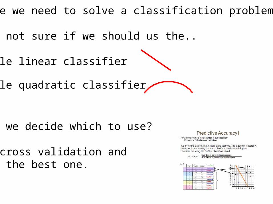
Suppose we need to solve a classification problem
We are not sure if we should us the..
• Simple linear classifier or the • Simple quadratic classifier
How do we decide which to use?
We do cross validation and choose the best one.

100
10 20 30 40 50 60 70 80 90 100
102030405060708090
100
10 20 30 40 50 60 70 80 90 100
102030405060708090
• Simple linear classifier gets 81% accuracy • Simple quadratic classifier 99% accuracy
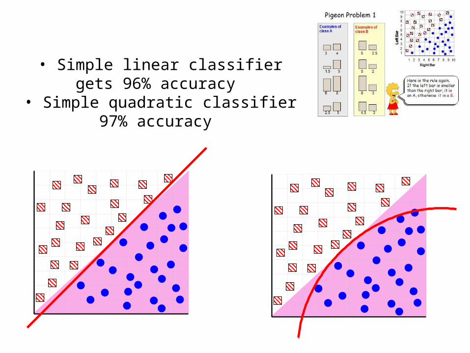
• Simple linear classifier gets 96% accuracy • Simple quadratic classifier 97% accuracy

This problem is greatly exacerbated by having too little data
• Simple linear classifier gets 90% accuracy • Simple quadratic classifier 95% accuracy
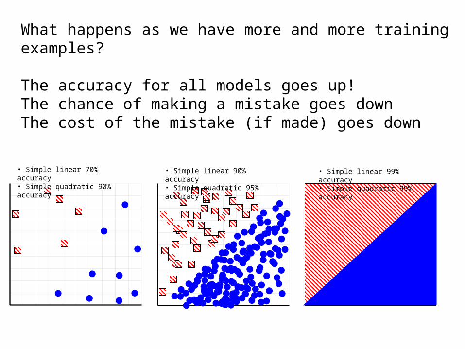
What happens as we have more and more training examples?
The accuracy for all models goes up!The chance of making a mistake goes downThe cost of the mistake (if made) goes down
• Simple linear 70% accuracy • Simple quadratic 90% accuracy
• Simple linear 90% accuracy • Simple quadratic 95% accuracy
• Simple linear 99% accuracy • Simple quadratic 99% accuracy
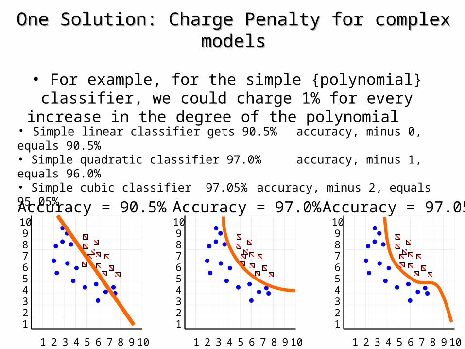
One Solution: Charge Penalty for complex modelsOne Solution: Charge Penalty for complex models
• For example, for the simple {polynomial} classifier, we could charge 1% for every increase in the degree of the polynomial
10
1 2 3 4 5 6 7 8 9 10
123456789
10
1 2 3 4 5 6 7 8 9 10
123456789
10
1 2 3 4 5 6 7 8 9 10
123456789
Accuracy = 90.5% Accuracy = 97.0% Accuracy = 97.05%
• Simple linear classifier gets 90.5% accuracy, minus 0, equals 90.5% • Simple quadratic classifier 97.0% accuracy, minus 1, equals 96.0% • Simple cubic classifier 97.05% accuracy, minus 2, equals 95.05%

One Solution: Charge Penalty for complex modelsOne Solution: Charge Penalty for complex models
• For example, for the simple {polynomial} classifier, we could charge 1% for every increase in the degree of the polynomial.
• There are more principled ways to charge penalties• In particular, there is a technique called Minimum Description Length (MDL)
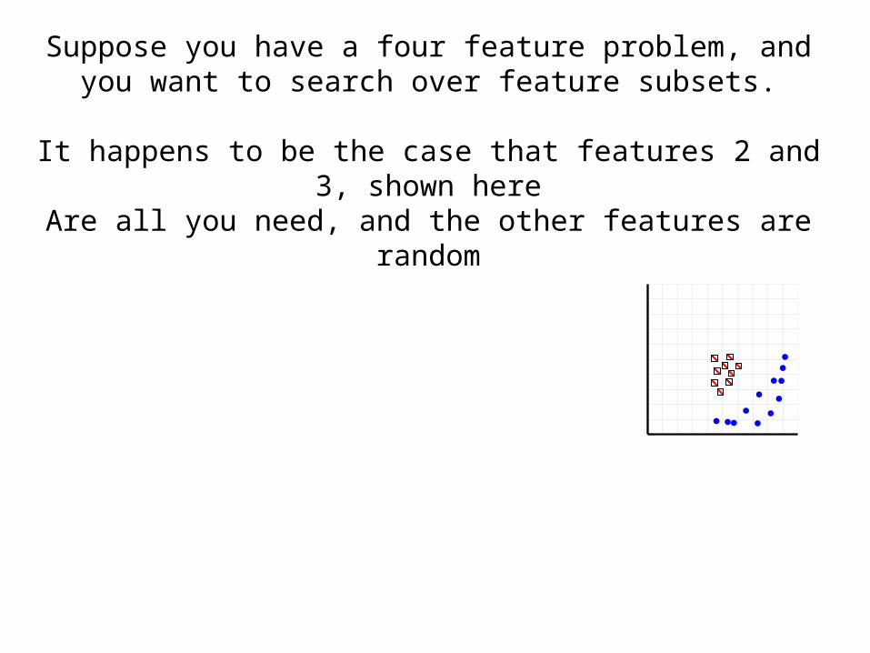
Suppose you have a four feature problem, and you want to search over feature subsets.
It happens to be the case that features 2 and 3, shown hereAre all you need, and the other features are random

Suppose you have a four feature problem, and you want to search over feature subsets.
It happens to be the case that features 2 and 3, shown hereare all you need, and the other features are random
1 2 3 4
3,42,41,42,31,31,2
2,3,41,3,41,2,41,2,3
1,2,3,4
0 1 2 3 4

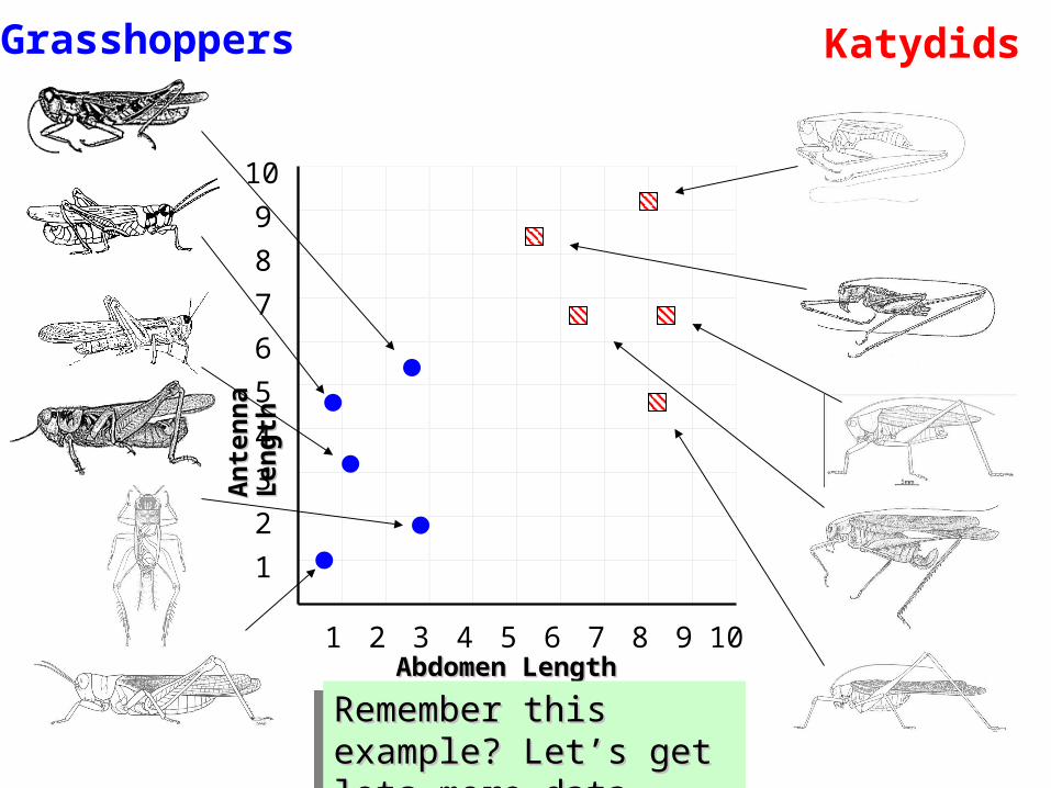
Insect Insect IDID
Abdomen Abdomen LengthLength
Antennae Antennae LengthLength
Insect Insect ClassClass
1 2.7 5.5 GrasshopperGrasshopper
2 8.0 9.1 KatydidKatydid
3 0.9 4.7 GrasshopperGrasshopper
4 1.1 3.1 GrasshopperGrasshopper
5 5.4 8.5 KatydidKatydid
6 2.9 1.9 GrasshopperGrasshopper
7 6.1 6.6 KatydidKatydid
8 0.5 1.0 GrasshopperGrasshopper
9 8.3 6.6 KatydidKatydid
10 8.1 4.7 KatydidsKatydids
My_CollectionMy_CollectionWe have seen that we We have seen that we
are given features…are given features…
Suppose using these Suppose using these features we cannot features we cannot get satisfactory get satisfactory accuracy results.accuracy results.
So far, we have two So far, we have two trickstricks
1)1) Ask for more featuresAsk for more features2)2) Remove irrelevant or Remove irrelevant or
redundant featuresredundant features
There is another possibility…There is another possibility…
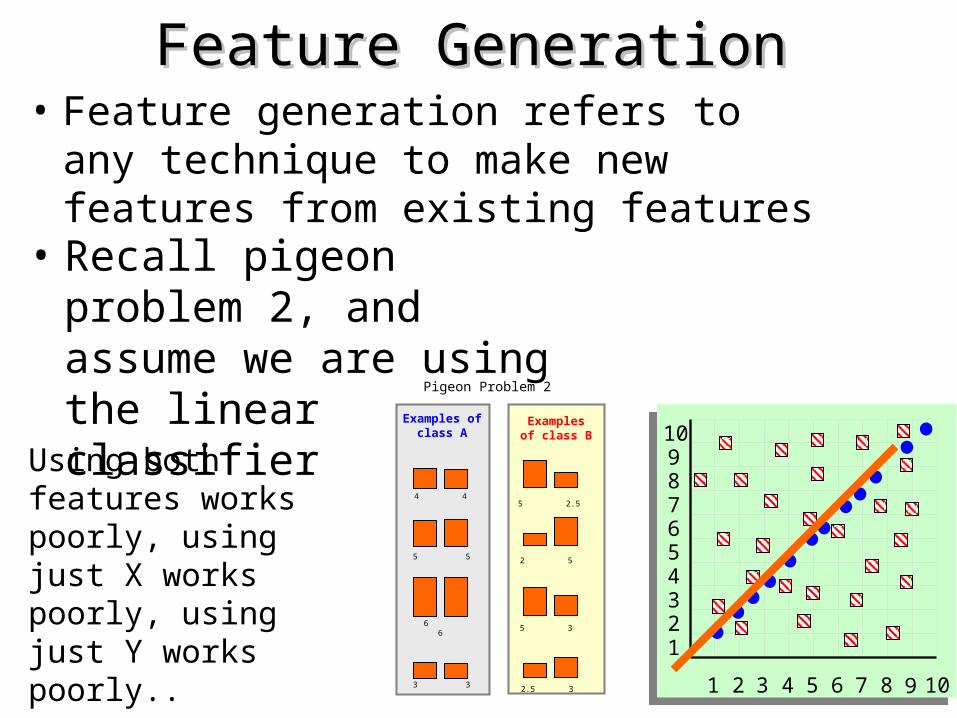
Feature GenerationFeature Generation• Feature generation refers to any technique
to make new features from existing features
10
1 2 3 4 5 6 7 8 9 10
123456789
• Recall pigeon problem 2, and assume we are using the linear classifier
Examples of class A
4 4
5 5
6 6
3 3
Examples of class B
5 2.5
2 5
5 3
2.5 3
Pigeon Problem 2
Using both features works poorly, using just X works poorly, using just Y works poorly..

Feature GenerationFeature Generation• Solution: Create a new feature Z
Z = absolute_value(X-Y)
10
1 2 3 4 5 6 7 8 9 10
123456789
1 2 3 4 5 6 7 8 9 100
Z-axis

Recall this example? It was a teaching example to show that Recall this example? It was a teaching example to show that NN could use any distance measureNN could use any distance measure
IDID NameName ClassClass
1 Gunopulos GreekGreek
2 Papadopoulos GreekGreek
3 Kollios GreekGreek
4 Dardanos GreekGreek
5 Keogh IrishIrish
6 Gough IrishIrish
7 Greenhaugh IrishIrish
8 Hadleigh IrishIrish
It would not really work very well, unless we had LOTS more data…

AIKO AIMI AINA
AIRI AKANE AKEMI
AKI AKIKO
AKIO AKIRA AMI AOI
ARATA ASUKA
ABERCROMBIE
ABERNETHY ACKART
ACKERMAN
ACKERS ACKLAND ACTON
ADAIR ADLAM
ADOLPH AFFLECK
ALVIN AMMADON
Japanese Names Irish Names

AIKO 0.75
AIMI 0.75
AINA 0.75
AIRI 0.75
AKANE 0.6
AKEMI 0.6
ABERCROMBIE 0.45
ABERNETHY 0.33
ACKART 0.33
ACKERMAN 0.375
ACKERS 0.33
ACKLAND 0.28
ACTON 0.33
Japanese Names Irish Names
Z = number of vowels / word length Vowels = I O U A E

I have a box of apples..I have a box of apples..A
ll bad
All good
0
0.5
1
H(X
)
Pr(X = good) = p then Pr(X = bad) = 1 − p the entropy of X is given by
0 1binary entropy function attains its maximum value when p = 0.5
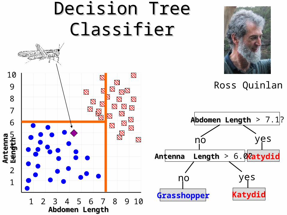
Decision Tree ClassifierDecision Tree Classifier
Ross Quinlan
An
tenn
a L
engt
hA
nte
nna
Len
gth
10
1 2 3 4 5 6 7 8 9 10
1
2
3
4
5
6
7
8
9
Abdomen LengthAbdomen Length
Abdomen LengthAbdomen Length > 7.1?
no yes
KatydidAntenna LengthAntenna Length > 6.0?
no yes
KatydidGrasshopper

Grasshopper
Antennae shorter than body?
Cricket
Foretiba has ears?
Katydids Camel Cricket
Yes
Yes
Yes
No
No
3 Tarsi?
No
Decision trees predate computers

• Decision tree – A flow-chart-like tree structure
– Internal node denotes a test on an attribute
– Branch represents an outcome of the test
– Leaf nodes represent class labels or class distribution
• Decision tree generation consists of two phases– Tree construction
• At start, all the training examples are at the root
• Partition examples recursively based on selected attributes
– Tree pruning
• Identify and remove branches that reflect noise or outliers
• Use of decision tree: Classifying an unknown sample– Test the attribute values of the sample against the decision tree
Decision Tree ClassificationDecision Tree Classification

• Basic algorithm (a greedy algorithm)– Tree is constructed in a top-down recursive divide-and-conquer manner– At start, all the training examples are at the root– Attributes are categorical (if continuous-valued, they can be discretized
in advance)– Examples are partitioned recursively based on selected attributes.– Test attributes are selected on the basis of a heuristic or statistical
measure (e.g., information gain)• Conditions for stopping partitioning
– All samples for a given node belong to the same class– There are no remaining attributes for further partitioning – majority
voting is employed for classifying the leaf– There are no samples left
How do we construct the decision tree?How do we construct the decision tree?

Information Gain as A Splitting CriteriaInformation Gain as A Splitting Criteria• Select the attribute with the highest information gain (information
gain is the expected reduction in entropy).
• Assume there are two classes, P and N
– Let the set of examples S contain p elements of class P and n elements of
class N
– The amount of information, needed to decide if an arbitrary example in S
belongs to P or N is defined as
np
n
np
n
np
p
np
pSE 22 loglog)(
0 log(0) is defined as 0

Information Gain in Decision Tree InductionInformation Gain in Decision Tree Induction
• Assume that using attribute A, a current set will be partitioned into some number of child sets
• The encoding information that would be gained by branching on A
)()()( setschildallEsetCurrentEAGain
Note: entropy is at its minimum if the collection of objects is completely uniform

Person Hair Length
Weight Age Class
Homer 0” 250 36 M
Marge 10” 150 34 F
Bart 2” 90 10 M
Lisa 6” 78 8 F
Maggie 4” 20 1 F
Abe 1” 170 70 M
Selma 8” 160 41 F
Otto 10” 180 38 M
Krusty 6” 200 45 M
Comic 8” 290 38 ?

Hair Length <= 5?yes no
Entropy(4F,5M) = -(4/9)log2(4/9) - (5/9)log2(5/9) = 0.9911
Entropy(1F,3M) = -(1/4)log2(1/4) - (3/4)log
2(3/4)
= 0.8113
Entropy(3F,2M) = -(3/5)log2(3/5) - (2/5)log
2(2/5)
= 0.9710
np
n
np
n
np
p
np
pSEntropy 22 loglog)(
Gain(Hair Length <= 5) = 0.9911 – (4/9 * 0.8113 + 5/9 * 0.9710 ) = 0.0911
)()()( setschildallEsetCurrentEAGain
Let us try splitting on Hair length
Let us try splitting on Hair length

Weight <= 160?yes no
Entropy(4F,5M) = -(4/9)log2(4/9) - (5/9)log2(5/9) = 0.9911
Entropy(4F,1M) = -(4/5)log2(4/5) - (1/5)log
2(1/5)
= 0.7219
Entropy(0F,4M) = -(0/4)log2(0/4) - (4/4)log
2(4/4)
= 0
np
n
np
n
np
p
np
pSEntropy 22 loglog)(
Gain(Weight <= 160) = 0.9911 – (5/9 * 0.7219 + 4/9 * 0 ) = 0.5900
)()()( setschildallEsetCurrentEAGain
Let us try splitting on Weight
Let us try splitting on Weight
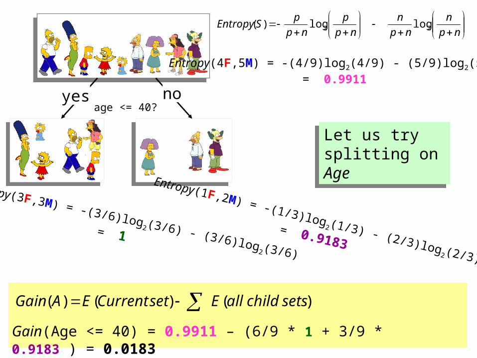
age <= 40?yes no
Entropy(4F,5M) = -(4/9)log2(4/9) - (5/9)log2(5/9) = 0.9911
Entropy(3F,3M) = -(3/6)log2(3/6) - (3/6)log
2(3/6)
= 1
Entropy(1F,2M) = -(1/3)log2(1/3) - (2/3)log
2(2/3)
= 0.9183
np
n
np
n
np
p
np
pSEntropy 22 loglog)(
Gain(Age <= 40) = 0.9911 – (6/9 * 1 + 3/9 * 0.9183 ) = 0.0183
)()()( setschildallEsetCurrentEAGain
Let us try splitting on Age
Let us try splitting on Age

Weight <= 160?yes no
Hair Length <= 2?yes no
Of the 3 features we had, Weight was best. But while people who weigh over 160 are perfectly classified (as males), the under 160 people are not perfectly classified… So we simply recurse!
This time we find that we can split on Hair length, and we are done!
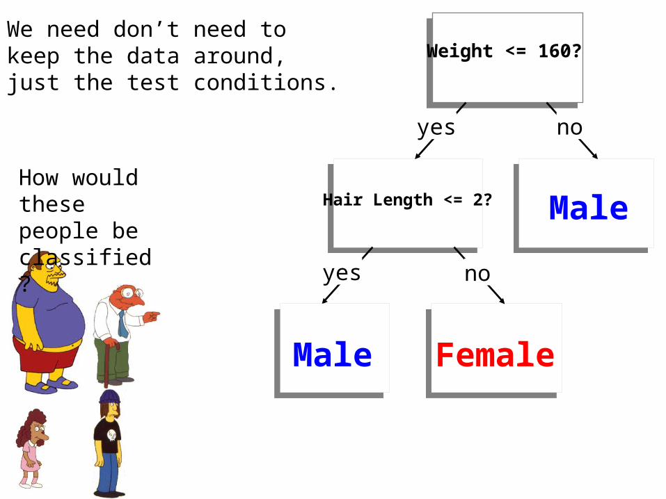
Weight <= 160?
yes no
Hair Length <= 2?
yes no
We need don’t need to keep the data around, just the test conditions.
Male
Male Female
How would these people be classified?

It is trivial to convert Decision Trees to rules…
Weight <= 160?
yes no
Hair Length <= 2?
yes no
Male
Male Female
Rules to Classify Males/Females
If Weight greater than 160, classify as MaleElseif Hair Length less than or equal to 2, classify as MaleElse classify as Female
Rules to Classify Males/Females
If Weight greater than 160, classify as MaleElseif Hair Length less than or equal to 2, classify as MaleElse classify as Female
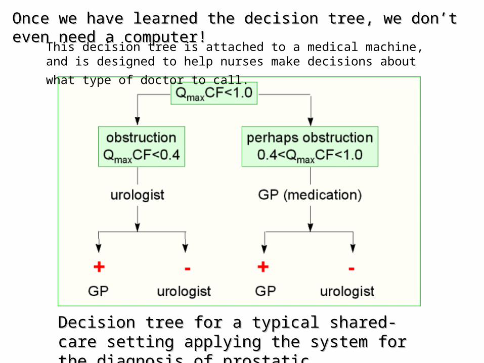
Decision tree for a typical shared-care setting applying Decision tree for a typical shared-care setting applying the system for the diagnosis of prostatic obstructions.the system for the diagnosis of prostatic obstructions.
Once we have learned the decision tree, we don’t even need a computer!Once we have learned the decision tree, we don’t even need a computer!
This decision tree is attached to a medical machine, and is designed to help
nurses make decisions about what type of doctor to call.

Garzotto M et al. JCO 2005;23:4322-4329
PSA = serum prostate-specific antigen levelsPSAD = PSA density
TRUS = transrectal ultrasound
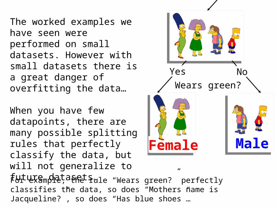
Wears green?
Yes No
The worked examples we have seen were performed on small datasets. However with small datasets there is a great danger of overfitting the data…
When you have few datapoints, there are many possible splitting rules that perfectly classify the data, but will not generalize to future datasets.
For example, the rule “Wears green?” perfectly classifies the data, so does “Mothers name is Jacqueline?”, so does “Has blue shoes”…
MaleFemale

Avoid Overfitting in ClassificationAvoid Overfitting in Classification• The generated tree may overfit the training data
– Too many branches, some may reflect anomalies due to noise or outliers
– Result is in poor accuracy for unseen samples
• Two approaches to avoid overfitting – Prepruning: Halt tree construction early—do not split a
node if this would result in the goodness measure falling below a threshold
• Difficult to choose an appropriate threshold– Postpruning: Remove branches from a “fully grown” tree
—get a sequence of progressively pruned trees• Use a set of data different from the training data to
decide which is the “best pruned tree”

10
1 2 3 4 5 6 7 8 9 10
123456789
100
10 20 30 40 50 60 70 80 90 100
10
20
30
40
50
60
70
80
90
10
1 2 3 4 5 6 7 8 9 10
123456789
Which of the “Pigeon Problems” can be Which of the “Pigeon Problems” can be solved by a Decision Tree?solved by a Decision Tree?
1)1) Deep Bushy TreeDeep Bushy Tree2)2) UselessUseless3)3) Deep Bushy TreeDeep Bushy Tree
The Decision Tree has a hard time with correlated attributes ?
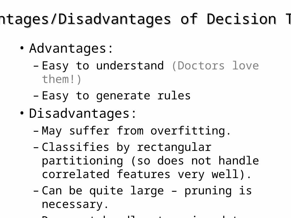
• Advantages:– Easy to understand (Doctors love them!) – Easy to generate rules
• Disadvantages:– May suffer from overfitting.– Classifies by rectangular partitioning (so does
not handle correlated features very well).– Can be quite large – pruning is necessary.– Does not handle streaming data easily
Advantages/Disadvantages of Decision TreesAdvantages/Disadvantages of Decision Trees

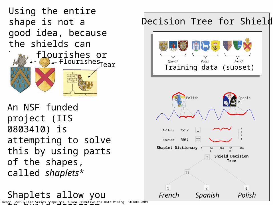
There now exists, perhaps tens of million of digitized pages of historical manuscripts dating back to the 12 th century, that feature one or more heraldic shields
The images are often stained, faded or torn

Wouldn’t it be great if we could automatically hyperlink all similar shields to each other?
For example, here we could link two occurrence of the Von Sax family shield.
To do this, we need to consider shape, color and texture. Lets just consider shape for now…
Manesse Codexan illuminated manuscript
in codex form, copied and illustrated between 1304 and 1340
in Zurich
0 100 200 300 400
0
1
2
3I
II
151.7
156.1
Shaplet Dictionary
I
II
Shield Decision Tree
2 01
Polish Spanish
(Polish)
(Spanish)
Spanish Polish French
Spanish PolishFrench
Training data (subset)
Using the entire shape is not a good idea, because the shields can have flourishes or tears
Flourishes Tear
An NSF funded project (IIS 0803410) is attempting to solve this by using parts of the shapes, called shaplets*
Shaplets allow you to build decision trees for shapes
*Ye and Keogh (2009) Time Series Shapelets: A New Primitive for Data Mining. SIGKDD 2009
Decision Tree for Shields


Naïve Bayes ClassifierNaïve Bayes Classifier
We will start off with a visual intuition, before looking at the math…
Thomas Bayes1702 - 1761
An
tenn
a L
engt
hA
nte
nna
Len
gth
10
1 2 3 4 5 6 7 8 9 10
1
2
3
4
5
6
7
8
9
Grasshoppers Katydids
Abdomen LengthAbdomen Length
Remember this example? Remember this example? Let’s get lots more data…Let’s get lots more data…
Remember this example? Remember this example? Let’s get lots more data…Let’s get lots more data…

An
tenn
a L
engt
hA
nte
nna
Len
gth
10
1 2 3 4 5 6 7 8 9 10
1
2
3
4
5
6
7
8
9
KatydidsGrasshoppers
With a lot of data, we can build a histogram. Let us With a lot of data, we can build a histogram. Let us just build one for “Antenna Length” for now…just build one for “Antenna Length” for now…

We can leave the histograms as they are, or we can summarize them with two normal distributions.
Let us us two normal distributions for ease of visualization in the following slides…

p(cj | d) = probability of class cj, given that we have observed dp(cj | d) = probability of class cj, given that we have observed d
3
Antennae length is 3
• We want to classify an insect we have found. Its antennae are 3 units long. How can we classify it?
• We can just ask ourselves, give the distributions of antennae lengths we have seen, is it more probable that our insect is a Grasshopper or a Katydid.• There is a formal way to discuss the most probable classification…

10
2
P(Grasshopper | 3 ) = 10 / (10 + 2) = 0.833
P(Katydid | 3 ) = 2 / (10 + 2) = 0.166
3
Antennae length is 3
p(cj | d) = probability of class cj, given that we have observed dp(cj | d) = probability of class cj, given that we have observed d

9
3
P(Grasshopper | 7 ) = 3 / (3 + 9) = 0.250
P(Katydid | 7 ) = 9 / (3 + 9) = 0.750
7
Antennae length is 7
p(cj | d) = probability of class cj, given that we have observed dp(cj | d) = probability of class cj, given that we have observed d

66
P(Grasshopper | 5 ) = 6 / (6 + 6) = 0.500
P(Katydid | 5 ) = 6 / (6 + 6) = 0.500
5
Antennae length is 5
p(cj | d) = probability of class cj, given that we have observed dp(cj | d) = probability of class cj, given that we have observed d
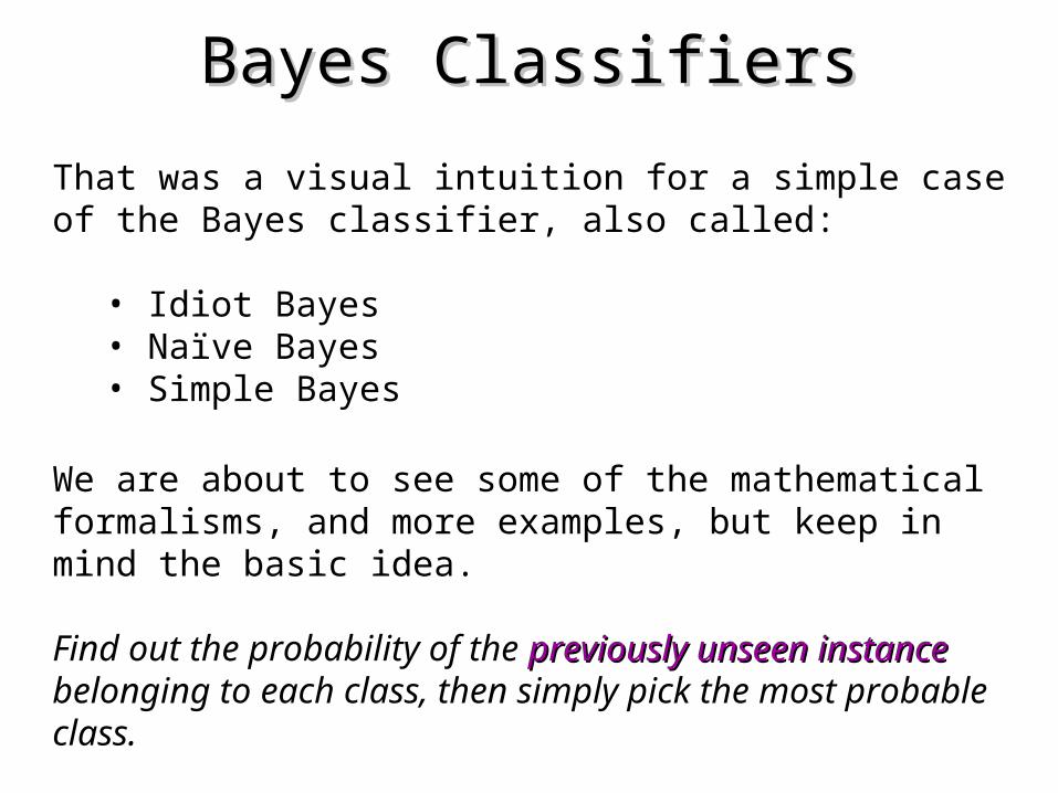
Bayes ClassifiersBayes Classifiers
That was a visual intuition for a simple case of the Bayes classifier, also called:
• Idiot Bayes • Naïve Bayes• Simple Bayes
We are about to see some of the mathematical formalisms, and more examples, but keep in mind the basic idea.
Find out the probability of the previously unseen instance previously unseen instance belonging to each class, then simply pick the most probable class.

Bayes ClassifiersBayes Classifiers• Bayesian classifiers use Bayes theorem, which says
p(cj | d ) = p(d | cj ) p(cj) p(d)
• p(cj | d) = probability of instance d being in class cj, This is what we are trying to compute
• p(d | cj) = probability of generating instance d given class cj,
We can imagine that being in class cj, causes you to have feature d with some probability
• p(cj) = probability of occurrence of class cj,
This is just how frequent the class cj, is in our database
• p(d) = probability of instance d occurring
This can actually be ignored, since it is the same for all classes

Assume that we have two classes
c1 = malemale, and c2 = femalefemale.
We have a person whose sex we do not know, say “drew” or d.
Classifying drew as male or female is equivalent to asking is it more probable that drew is malemale or femalefemale, I.e which is greater p(malemale | drew) or p(femalefemale | drew)
p(malemale | drew) = p(drew | malemale ) p(malemale)
p(drew)
(Note: “Drew can be a male or female name”)
What is the probability of being called “drew” given that you are a male?
What is the probability of being a male?
What is the probability of being named “drew”? (actually irrelevant, since it is that same for all classes)
Drew Carey
Drew Barrymore

p(cj | d) = p(d | cj ) p(cj)
p(d)
Officer Drew
Name Sex
Drew MaleMale
Claudia FemaleFemale
Drew FemaleFemale
Drew FemaleFemale
Alberto MaleMale
Karin FemaleFemale
Nina FemaleFemale
Sergio MaleMale
This is Officer Drew (who arrested me in This is Officer Drew (who arrested me in 1997). Is Officer Drew a 1997). Is Officer Drew a MaleMale or or FemaleFemale??
Luckily, we have a small database with names and sex.
We can use it to apply Bayes rule…
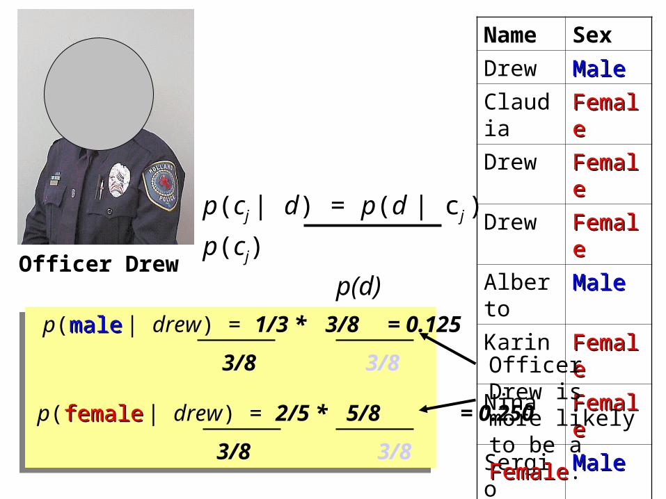
p(malemale | drew) = 1/3 * 3/8 = 0.125
3/8 3/8
p(femalefemale | drew) = 2/5 * 5/8 = 0.250
3/8 3/8
Officer Drew
p(cj | d) = p(d | cj ) p(cj)
p(d)
Name Sex
Drew MaleMale
Claudia FemaleFemale
Drew FemaleFemale
Drew FemaleFemale
Alberto MaleMale
Karin FemaleFemale
Nina FemaleFemale
Sergio MaleMale
Officer Drew is more likely to be a FemaleFemale.

Officer Drew IS a female!Officer Drew IS a female!
Officer Drew
p(malemale | drew) = 1/3 * 3/8 = 0.125
3/8 3/8
p(femalefemale | drew) = 2/5 * 5/8 = 0.250
3/8 3/8

Name Over 170CM Eye Hair length Sex
Drew No Blue Short MaleMale
Claudia Yes Brown Long FemaleFemale
Drew No Blue Long FemaleFemale
Drew No Blue Long FemaleFemale
Alberto Yes Brown Short MaleMale
Karin No Blue Long FemaleFemale
Nina Yes Brown Short FemaleFemale
Sergio Yes Blue Long MaleMale
p(cj | d) = p(d | cj ) p(cj)
p(d)
So far we have only considered Bayes Classification when we have one attribute (the “antennae length”, or the “name”). But we may have many features.How do we use all the features?

• To simplify the task, naïve Bayesian classifiers assume attributes have independent distributions, and thereby estimate
p(d|cj) = p(d1|cj) * p(d2|cj) * ….* p(dn|cj)
The probability of class cj generating instance d, equals….
The probability of class cj generating the observed value for feature 1, multiplied by..
The probability of class cj generating the observed value for feature 2, multiplied by..

• To simplify the task, naïve Bayesian classifiers assume attributes have independent distributions, and thereby estimate
p(d|cj) = p(d1|cj) * p(d2|cj) * ….* p(dn|cj)
p(officer drew|cj) = p(over_170cm = yes|cj) * p(eye =blue|cj) * ….
Officer Drew is blue-eyed, over 170cm tall, and has long hair
p(officer drew| FemaleFemale) = 2/5 * 3/5 * ….
p(officer drew| MaleMale) = 2/3 * 2/3 * ….
p(d1|cj) p(d2|cj) p(dn|cj)
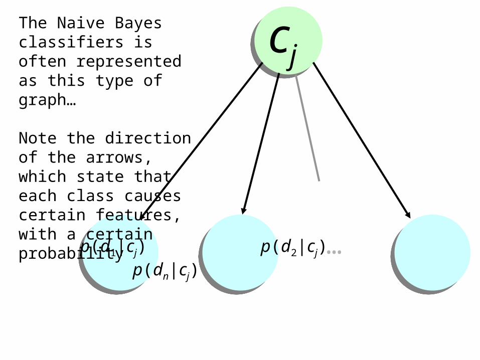
cjThe Naive Bayes classifiers is often represented as this type of graph…
Note the direction of the arrows, which state that each class causes certain features, with a certain probability
…

Naïve Bayes is fast and Naïve Bayes is fast and space efficientspace efficient
We can look up all the probabilities with a single scan of the database and store them in a (small) table…
Sex Over190cm
MaleMale Yes 0.15
No 0.85
FemaleFemale Yes 0.01
No 0.99
cj
…p(d1|cj) p(d2|cj) p(dn|cj)
Sex Long Hair
MaleMale Yes 0.05
No 0.95
FemaleFemale Yes 0.70
No 0.30
Sex
MaleMale
FemaleFemale

Naïve Bayes is NOT sensitive to irrelevant features...Naïve Bayes is NOT sensitive to irrelevant features...
Suppose we are trying to classify a persons sex based on several features, including eye color. (Of course, eye color is completely irrelevant to a persons gender)
p(Jessica | FemaleFemale) = 9,000/10,000 * 9,975/10,000 * ….
p(Jessica | MaleMale) = 9,001/10,000 * 2/10,000 * ….
p(Jessica |cj) = p(eye = brown|cj) * p( wears_dress = yes|cj) * ….
However, this assumes that we have good enough estimates of the probabilities, so the more data the better.
Almost the same!

An obvious pointAn obvious point. I have used a . I have used a simple two class problem, and simple two class problem, and two possible values for each two possible values for each example, for my previous example, for my previous examples. However we can have examples. However we can have an arbitrary number of classes, or an arbitrary number of classes, or feature valuesfeature values
Animal Mass >10kg
CatCat Yes 0.15
No 0.85
DogDog Yes 0.91
No 0.09
PigPig Yes 0.99
No 0.01
cj
…p(d1|cj) p(d2|cj) p(dn|cj)
Animal
CatCat
DogDog
PigPig
Animal Color
CatCat Black 0.33
White 0.23
Brown 0.44
DogDog Black 0.97
White 0.03
Brown 0.90
PigPig Black 0.04
White 0.01
Brown 0.95

Naïve Bayesian Naïve Bayesian ClassifierClassifier
p(d1|cj) p(d2|cj) p(dn|cj)
p(d|cj)Problem!
Naïve Bayes assumes independence of features…
Sex Over 6 foot
Male Yes 0.15
No 0.85
Female Yes 0.01
No 0.99
Sex Over 200 pounds
Male Yes 0.11
No 0.80
Female Yes 0.05
No 0.95

Naïve Bayesian Naïve Bayesian ClassifierClassifier
p(d1|cj) p(d2|cj) p(dn|cj)
p(d|cj)Solution
Consider the relationships between attributes…
Sex Over 6 foot
Male Yes 0.15
No 0.85
Female Yes 0.01
No 0.99
Sex Over 200 pounds
Male Yes and Over 6 foot 0.11
No and Over 6 foot 0.59
Yes and NOT Over 6 foot 0.05
No and NOT Over 6 foot 0.35
Female Yes and Over 6 foot 0.01

Naïve Bayesian Naïve Bayesian ClassifierClassifier
p(d1|cj) p(d2|cj) p(dn|cj)
p(d|cj)Solution
Consider the relationships between attributes…
But how do we find the set of connecting arcs??

The Naïve Bayesian Classifier has a piecewise quadratic decision boundaryThe Naïve Bayesian Classifier has a piecewise quadratic decision boundary
GrasshoppersKatydids
Ants
Adapted from slide by Ricardo Gutierrez-Osuna

10
1 2 3 4 5 6 7 8 9 10
123456789
100
10 20 30 40 50 60 70 80 90 100
10
20
30
40
50
60
70
80
90
10
1 2 3 4 5 6 7 8 9 10
123456789
Which of the “Pigeon Problems” can be Which of the “Pigeon Problems” can be solved by a decision tree?solved by a decision tree?

Dear SIR,
I am Mr. John Coleman and my sister is Miss Rose Colemen, we are the children of late Chief Paul Colemen from Sierra Leone. I am writing you in absolute confidence primarily to seek your assistance to transfer our cash of twenty one Million Dollars ($21,000.000.00) now in the custody of a private Security trust firm in Europe the money is in trunk boxes deposited and declared as family valuables by my late father as a matter of fact the company does not know the content as money, although my father made them to under stand that the boxes belongs to his foreign partner.…

This mail is probably spam. The original message has been attached along with this report, so you can recognize or block similar unwanted mail in future. See http://spamassassin.org/tag/ for more details.
Content analysis details: (12.20 points, 5 required)NIGERIAN_SUBJECT2 (1.4 points) Subject is indicative of a Nigerian spamFROM_ENDS_IN_NUMS (0.7 points) From: ends in numbersMIME_BOUND_MANY_HEX (2.9 points) Spam tool pattern in MIME boundaryURGENT_BIZ (2.7 points) BODY: Contains urgent matterUS_DOLLARS_3 (1.5 points) BODY: Nigerian scam key phrase ($NN,NNN,NNN.NN)DEAR_SOMETHING (1.8 points) BODY: Contains 'Dear (something)'BAYES_30 (1.6 points) BODY: Bayesian classifier says spam probability is 30 to 40% [score: 0.3728]
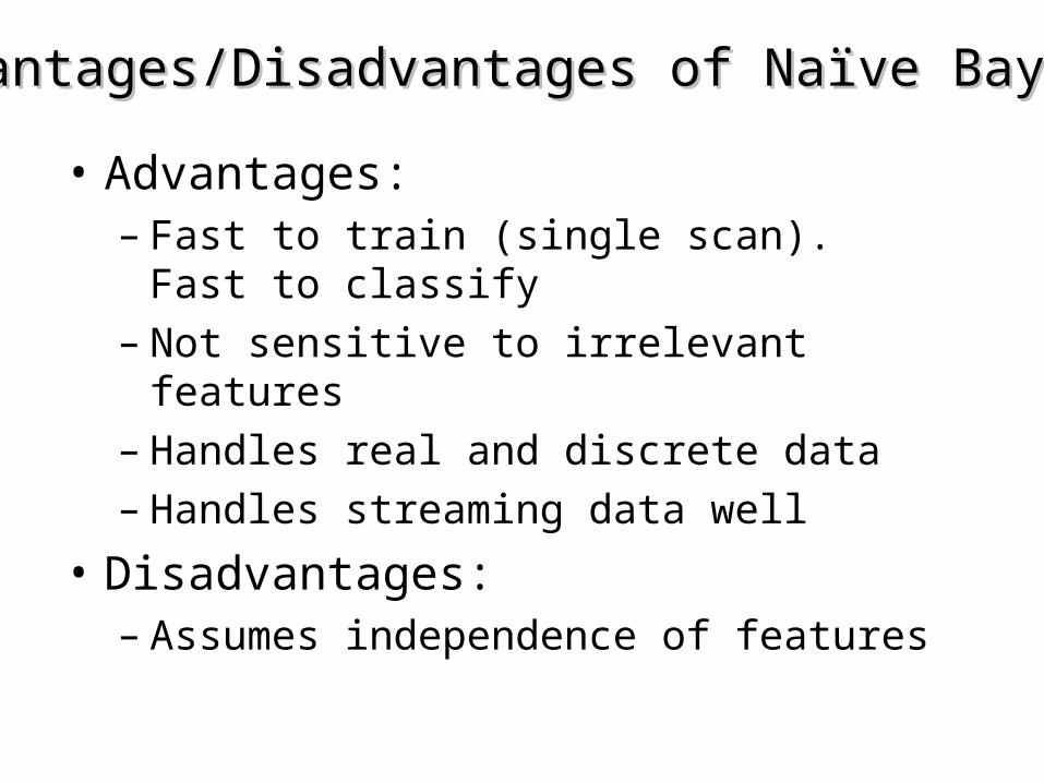
• Advantages:– Fast to train (single scan). Fast to classify – Not sensitive to irrelevant features– Handles real and discrete data– Handles streaming data well
• Disadvantages:– Assumes independence of features
Advantages/Disadvantages of Naïve BayesAdvantages/Disadvantages of Naïve Bayes
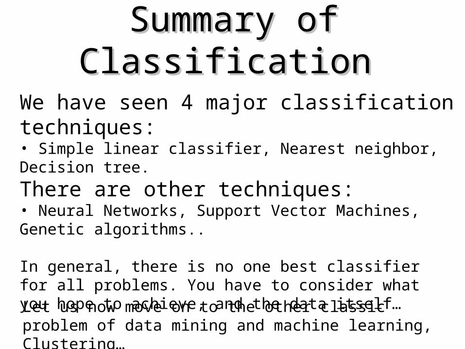
Summary of ClassificationSummary of Classification
We have seen 4 major classification techniques:• Simple linear classifier, Nearest neighbor, Decision tree.
There are other techniques:• Neural Networks, Support Vector Machines, Genetic algorithms..
In general, there is no one best classifier for all problems. You have to consider what you hope to achieve, and the data itself…
Let us now move on to the other classic problem of data mining and machine learning, Clustering…