Automatica 46 (2010) 1524–1530

Contents lists available at ScienceDirect

Automatica

journal homepage: www.elsevier.com/locate/automatica

Brief paper

Output feedback pole placement for linear time-varying systems withapplication to the control of nonlinear systemsI

Bogdan Marinescu ∗SATIE, Ecole Normale Supérieure de Cachan, 61, avenue du Président Wilson, 94230 Cachan, France

a r t i c l e i n f o

Article history:Received 11 August 2009Received in revised form15 April 2010Accepted 21 May 2010Available online 10 July 2010

Keywords:Linear time-varying systemsNonlinear systemsOutput feedback pole placementStability

a b s t r a c t

The output feedback pole placement problem is solved in an input–output algebraic formalism for lineartime-varying (LTV) systems. The recent extensions of the notions of transfer matrices and poles of thesystem to the case of LTV systems are exploited here to provide constructive solutions based, as in thelinear time-invariant (LTI) case, on the solutions of diophantine equations. Also, differences with theresults known in the LTI case are pointed out, especially concerning the possibilities to assign specificdynamics to the closed-loop system and the conditions for tracking and disturbance rejection. Thisapproach is applied to the control of nonlinear systems by linearization around a given trajectory. Severalexamples are treated in detail to show the computation and implementation issues.

© 2010 Elsevier Ltd. All rights reserved.

1. Introduction

The feedback pole placement problem consists in regulatingthe natural response of a system using measures of some ofits variables. The case of linear time-varying (LTV) systems isimportant since this situation is encountered not only when oneor some parameters of the system may, due to the physics of theprocess, vary with time, but also when the system to be controlledis nonlinear and the problem is approached by linearizing thissystem around a given trajectory which leads to an LTV system.Most of the existing results for dynamics assignment in the LTV

case were obtained by reducing a state-space representation tothe (right) canonical form and, next choosing time-varying state-feedback gains in order to place constant poles to the closed-loop system (e.g., Rotella, 2003; Valášek & Olgac, 1999). First,it is well known that the transformation to a canonical form isnot robust for ill-conditioned matrices. Next, as is shown in thepresent paper, the structure of the set of the poles of a closed-loopsystem is more complex in the LTV case and, imposing constantpoles for one of the transfers of the closed-loop do not necessarilyensure time-invariant poles for the closed-loop system. Thus, animportant part of the work reported here assesses the analysis

I The material in this paper was not presented at any conference. This paper wasrecommended for publication in revised form by Associate Editor Tong Zho underthe direction of Editor Roberto Tempo.∗ Tel.: +33 1 39244017; fax: +33 1 39244175.E-mail addresses: bogdanmarinescu@hotmail.fr,

bogdan.marinescu@satie.ens-cachan.fr.

0005-1098/$ – see front matter© 2010 Elsevier Ltd. All rights reserved.doi:10.1016/j.automatica.2010.06.022

of the internal stability of an output feedback LTV closed-loopsystem. It is clarified what dynamics can be assigned by LTV poleplacement in comparison to the linear time-invariant (LTI) case.For this, the notions of poles of an LTV system, newly introduced inMarinescu andBourlès (2009) alongwith a necessary and sufficientcondition for exponential stability, are exploited to study theinternal stability of the output closed-loop system. Moreover, it isshown how the pole placement problem can be effectively solved,i.e., how the regulator synthesis and implementation can be doneand how this kind of LTV regulator can be used for the control ofboth linear and nonlinear systems.Several input–output descriptions have been introduced in the

late 80s for LTV systems (Emre, Tai, & Seo, 1990; Fliess, 1990; Ka-men, Khargonekar, & Poolla, 1985). Here, the transfer function ap-proach of Fliess (1990) is used to solve the output feedback poleplacement problem for LTV systems defined over a field. The otherinput–output representations mentioned above have been usedin Emre et al. (1990) and Poola and Khargonekar (1987) to studythe output feedback problem for LTV systems with coefficients ina ring. In comparison to Emre et al. (1990) and Poola and Khar-gonekar (1987), the formalism used in Fliess (1990) andMarinescuand Bourlès (2009) for the LTV systems defined over fields allowedus to ensure better in the present paper, the stability of the closed-loop system and to give effective computation algorithms for thesynthesis of the regulator. It is thus provided a general solution ofthe problem tackled in some particular cases of LTV systems de-fined over fields in Guglielmi (2002) and Zhu, Johnson, Thompson,and Wendt (1990). This has facilitated applications to real (phys-ical) systems and extensions to the control of nonlinear systemswhich are presented in the last part of this paper.

B. Marinescu / Automatica 46 (2010) 1524–1530 1525

The paper is organized as follows: in Section 2, backgroundnotions along with some key results obtained in Marinescu andBourlès (2009) on the poles and stability of LTV systems are re-called. Technical results on the factorization and the poles of LTVtransfer matrices are established in Section 3. The pole placementis explained in Section 4 while the next 2 sections are devoted tothe applications to the synthesis of a two-parameter (or a two-degrees-of-freedom) compensator and to the nonlinear control.Section 7 contains concluding remarks.

2. Background notions

2.1. LTV systems

In the algebraic framework initiated byMalgrange (1962–1963)and popularized in systems theory by Fliess (1990) and relatedreferences, a linear system is a finitely presented module M overthe ring R = K[s] of differential operators in s = d/dt withcoefficients in an ordinary differential field K (i.e., a commutativefield equipped with a unique derivative). If K does not exclusivelycontain constants (i.e., elements of derivative zero), M is an LTVsystem. An input ofM is a set of variables u = (ui)i=1,...,m such that[u]R, the R-module generated by the entries of u, is free of rank mand M/[u]R is torsion. If an output y = (yi)i=1,...,p is also chosen,a state variable description can also be given for the input–outputsystem (M, u, y).

2.2. Stability

2.2.1. Autonomous systemsThe so-called autonomous part of the system is obtained by can-

celing the input variables; algebraically, this corresponds to thetorsion module T ∼= M/[u]R. As R is simple, T is cyclic and canbe characterized by a scalar differential equation

P(s)y = 0, P(s) = sn +n−1∑i=0

aisi (1)

where y is a generator of T .

2.2.2. Noncommutative algebra (Cohn, 1985)When dealing with LTV systems, polynomial P(s) in (1) is skew,

i.e., belongs to the noncommutative ring R = K[s] equipped withthe commutation rulesa = as+ a (2)which is the Leibniz rule of derivation of a product. The evaluationof P in α ∈ K, denoted by P(α) is defined as follows: P(α) =Nn(α)+

∑n−1i=0 aiNi(α)where Ni is defined inductively by N0(α) =

1, Ni(α) = Ni−1(α)α + ddt (Ni−1(α)). P(α) = 0 if, and only if (iff),

s − α is a right factor of P(s) and, in this case, we say that α is a(right) root or zero of P . For any 0 6= c ∈ K, the conjugate of α by c,denoted by αc , is αc = α + cc−1. ∆K(α) = {α

c, c ∈ K, c 6= 0} iscalled the conjugacy class of α over K. A product formula

(PG)(α) = 0, if G(α) = 0; P(αG(α))G(α), if G(α) 6= 0 (3)as well as left and right greatest common divisors (GCD) and leastcommon multiples (LCM) exist for skew polynomials. They can bealso extended to matrices: matrices A(s), B(s) are said left (resp.right) coprime if their left (resp. right) GCDs are unimodular. Forpolynomials, the left LCM, denoted by [P,G]l, can be computed forfirst order factors using (3):

[P(s), s− α]l = P(s), if P(α) = 0

[P(s), s− α]l = (s− αP(α))P(s), if P(α) 6= 0.(4)

Let ∆ = {γ1, . . . , γn} ⊆ K. The minimal polynomial of ∆, denotedby P∆ is P∆(s) = [s − γi, i = 1, . . . , n]l. ∆ is said P-independent

if the degree of P∆ is n. A skew polynomial P of degree n has aninfinite number of roots which lie in at most n conjugacy classes.To characterize stability, we are interested in a fundamental set ofroots of P in (1), i.e., a set of n P-independent roots of P (Marinescu& Bourlès, 2009).

Example 1. P(s) = (s − t)2. Obviously t is a root, but {t, t} arenot P-independent. From the double root t one can compute onefundamental set of roots, for example {t, t + t−1} following theprocedure introduced in Marinescu and Bourlès (2009). �

The elements γi of a fundamental set of roots are in directrelation with the elements yi of a fundamental set of solutions ofthe differential equation (1): yiy−1i = γi. For Example 1, obviously,y1 = e

∫γ1(t)dt = et

2/2, y2 = e∫γ2(t)dt = tet

2/2 is a fundamental setof solutions of P(s)y = 0. Notice also that a fundamental set of rootsof P does not always exist over K, the initial field of definition ofthe system, in which case a field extension Kmust be constructed(Marinescu & Bourlès, 2009).

2.2.3. Poles and stability (Marinescu & Bourlès, 2009)Consider an autonomous LTV system given by the torsion

R-module T ∼= R/RP(s).

Definition 1. Let γi ∈ K, i = 1, . . . , n be a fundamental setof roots of the polynomial P(s). The poles of T are the conjugacyclasses {∆K(γi), i = 1, . . . , n}. A set {γ 1, . . . , γ n} of representa-tives of these poles (i.e., γ i ∈ ∆K(γi)) is called fundamental if theγ i’s are P-independent, i.e., if they form a fundamental set of roots.Themodule of poles of T is T ∼= R/RP(s) ∼= ⊕i R/R(s− γi) obtainedfrom T by the extension of the ring of scalars to R = K[s]. �

For Example 1, T ∼= R/R(s− t)⊕ R/R(s− t − t−1).Representation (1) is not unique. Indeed, a given autonomous

system can also be defined by P(s)y = 0 if R/RP ∼= R/RP . In thiscase, P and P are said similar (Cohn, 1985), written P(s) ∼ P(s).In Marinescu and Bourlès (2009), the choice K = C((t)) (i.e., thefield of Laurent series with complex coefficients) has facilitatedpolynomial factorizations from which fundamental sets of rootswere obtained. The field extensions K in this case are of the formC((t1/m)) for somem ∈ N. However, in practice, the description ofphysical phenomena do not need infinite series coefficients, so wecan limit to a more realistic choice of fields of rational functionsK = C(t). To allow the field extensions above, the Puiseux-typefield K∞ =

⋃m≥1 C(t1/m) has been considered in Marinescu and

Bourlès (2009). One has the following results:

Proposition 1. If K ⊆ K∞, then limt→+∞[γ (t) − γ (t)] = 0,∀γ i(t) ∈ ∆K(γi). �

Proof. The result is obvious using the fact that limt→+∞ c(t)c−1(t)= 0 when c(t) is of rational type. �

Theorem 1. If {γ1, . . . , γn} ∈ K ⊆ K∞ is a fundamental setof representatives of poles of T , then T is exponentially stable ifflimt→+∞ Re{γi} < 0, i = 1, . . . , n. �

3. Transfer matrices

3.1. Factorizations and implementation

R = K[s] is an Euclidean domain thus a two-sided Ore domainand it has a field of left fractions and a field of right fractions whichcoincide (see Bourlès, 2005; Cohn, 1985); this field is denoted

1526 B. Marinescu / Automatica 46 (2010) 1524–1530

by Q = K(s). A transfer matrix of an input–output LTV system(M, u, y) is a matrix with entries in Q (Fliess, 1990). The followingnotations are used in the sequel to denote matrices: H (or H(t))is a matrix with entries in K,H(s) a matrix with entries in R (apolynomial matrix) andH(s) a matrix with entries in Q (a transfermatrix). The GCDs recalled in Section 2 lead to the followingfactorizations of a given LTV transfer matrix (Fliess, 1990):

Proposition 2. Any LTV transfer matrixH(s) has:(i) left coprime factorizations: H(s) = AL(s)−1BL(s), where AL(s)and BL(s) are left coprime, i.e., AL(s)y = BL(s)u

(ii) right coprime factorizations:H(s) = BR(s)AR(s)−1, where AR(s)and BR(s) are right coprime, i.e., y = BR(s)ξ and u = AR(s)ξ

related by the diophantine equation

AL(s)BR(s)− BL(s)AR(s) = 0. (5)

Two left (resp. right) coprime factorizationsH(s) = AL(s)−1BL(s)= A

−1L (s)BL(s) (resp. H(s) = BR(s)AR(s)

−1= BR(s)AR(s)−1) are

equivalent in the sense that it exists an unimodular matrix U(s)with entries in R and of appropriate dimensions such that AL(s) =U(s)AL(s), BL(s) = U(s)BL(s) (resp. AR(s) = AR(s)U(s), BR(s) =BR(s)U(s)). �

Factorizations (i) and (ii) lead to the right and left statecanonical forms as in the LTI case. They are important for thepractical implementation of the regulator since they provide asystematic way to ensure causality in the input/output relations,i.e., schemes which contain only integrators. To derive them inthe LTV case, the commutation rule (2) is used. For example, forH(s) = AL(s)−1BL(s), AL(s) = sn + an−1sn−1 + · · · + a0, BL(s) =bnsn + bn−1sn−1 + · · · + b0 and ai, bj ∈ K, one can write AL(s) =sn+sn−1an−1+· · ·+a0 and BL(s) = snbn+sn−1bn−1+· · ·+b0 fromwhich follows y = bnu+s−1(bn−1u−an−1y)+· · ·+s−n(b0u−a0y)which is a causal description ofH(s). To the latter expression cor-responds the left (observable) canonical form state formofH(s). Thedual right (controllable) form is obtained in a similar way from afactorization (ii) ofH(s).

3.2. Transmission poles

The transmission poles, as introduced in Bourlès and Fliess(1997) for LTI systems and extended in Marinescu and Bourlès(2009) to the case of LTV systems, are used to evaluate the stabilityof an input–output LTV system given by a transfer matrixH(s). If afactorization (i) is used, themodule of transmission poles is definedby AL(s)y = 0 (where y is the image of the output y in the moduleof the transmission poles). Starting from (ii), the same module isdefined by AR(s)ξ = 0. It follows

Proposition 3. Consider factorizations (i) and (ii) of a transfermatrix: H(s) = AL(s)−1BL(s) = BR(s)AR(s)−1. Then AL(s) andAR(s) are definition matrices of the module of transmissionpoles ofH(s). Moreover, P(s) ∼ P(s) where AL(s) ∼ {1, . . . , 1, P(s)} andAR(s) ∼ {1, . . . , 1, P(s)} are the Jacobson–Teichmüller forms (Cohn,1985) of AL(s) and AR(s) respectively. �

A transfer matrix of which poles belong to K∞ and satisfythe condition of Theorem 1 is called exponentially stable. For atransfer function, obviously the transmission poles are the roots ofpolynomials AL(s) and AR(s).

4. Output feedback pole placement

4.1. Closed-loop transfer matrices and stability

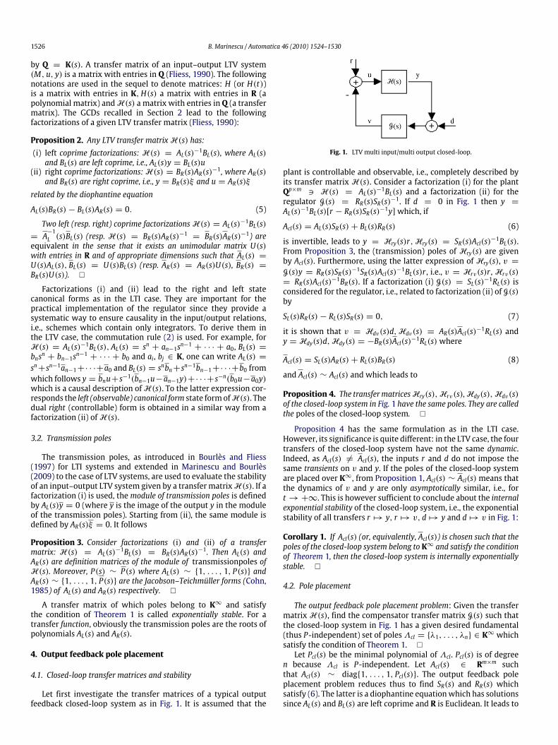
Let first investigate the transfer matrices of a typical outputfeedback closed-loop system as in Fig. 1. It is assumed that the

Fig. 1. LTV multi input/multi output closed-loop.

plant is controllable and observable, i.e., completely described byits transfer matrix H(s). Consider a factorization (i) for the plantQp×m 3 H(s) = AL(s)−1BL(s) and a factorization (ii) for theregulator G(s) = RR(s)SR(s)−1. If d = 0 in Fig. 1 then y =AL(s)−1BL(s)[r − RR(s)SR(s)−1y]which, if

Acl(s) = AL(s)SR(s)+ BL(s)RR(s) (6)

is invertible, leads to y = Hry(s)r,Hry(s) = SR(s)Acl(s)−1BL(s).From Proposition 3, the (transmission) poles of Hry(s) are givenby Acl(s). Furthermore, using the latter expression of Hry(s), v =G(s)y = RR(s)SR(s)−1SR(s)Acl(s)−1BL(s)r , i.e., v = Hrv(s)r , Hrv(s)= RR(s)Acl(s)−1BR(s). If a factorization (i) G(s) = SL(s)−1RL(s) isconsidered for the regulator, i.e., related to factorization (ii) of G(s)by

SL(s)RR(s)− RL(s)SR(s) = 0, (7)

it is shown that v = Hdv(s)d,Hdv(s) = AR(s)Acl(s)−1RL(s) andy = Hdy(s)d,Hdy(s) = −BR(s)Acl(s)−1RL(s)where

Acl(s) = SL(s)AR(s)+ RL(s)BR(s) (8)

and Acl(s) ∼ Acl(s) and which leads to

Proposition 4. The transfermatricesHry(s),Hrv(s),Hdy(s),Hdv(s)of the closed-loop system in Fig. 1 have the same poles. They are calledthe poles of the closed-loop system. �

Proposition 4 has the same formulation as in the LTI case.However, its significance is quite different: in the LTV case, the fourtransfers of the closed-loop system have not the same dynamic.Indeed, as Acl(s) 6= Acl(s), the inputs r and d do not impose thesame transients on v and y. If the poles of the closed-loop systemare placed over K∞, from Proposition 1, Acl(s) ∼ Acl(s)means thatthe dynamics of v and y are only asymptotically similar, i.e., fort →+∞. This is however sufficient to conclude about the internalexponential stability of the closed-loop system, i.e., the exponentialstability of all transfers r 7→ y, r 7→ v, d 7→ y and d 7→ v in Fig. 1:

Corollary 1. If Acl(s) (or, equivalently, Acl(s)) is chosen such that thepoles of the closed-loop system belong to K∞ and satisfy the conditionof Theorem 1, then the closed-loop system is internally exponentiallystable. �

4.2. Pole placement

The output feedback pole placement problem: Given the transfermatrix H(s), find the compensator transfer matrix G(s) such thatthe closed-loop system in Fig. 1 has a given desired fundamental(thus P-independent) set of polesΛcl = {λ1, . . . , λn} ∈ K∞ whichsatisfy the condition of Theorem 1. �Let Pcl(s) be the minimal polynomial of Λcl. Pcl(s) is of degree

n because Λcl is P-independent. Let Acl(s) ∈ Rm×m suchthat Acl(s) ∼ diag{1, . . . , 1, Pcl(s)}. The output feedback poleplacement problem reduces thus to find SR(s) and RR(s) whichsatisfy (6). The latter is a diophantine equationwhich has solutionssince AL(s) and BL(s) are left coprime and R is Euclidean. It leads to

B. Marinescu / Automatica 46 (2010) 1524–1530 1527

1

0.5

0

-0.5

y1 -

and

y2

--

0 2 4 6 8 10time t in sec

12 14 16 18 20

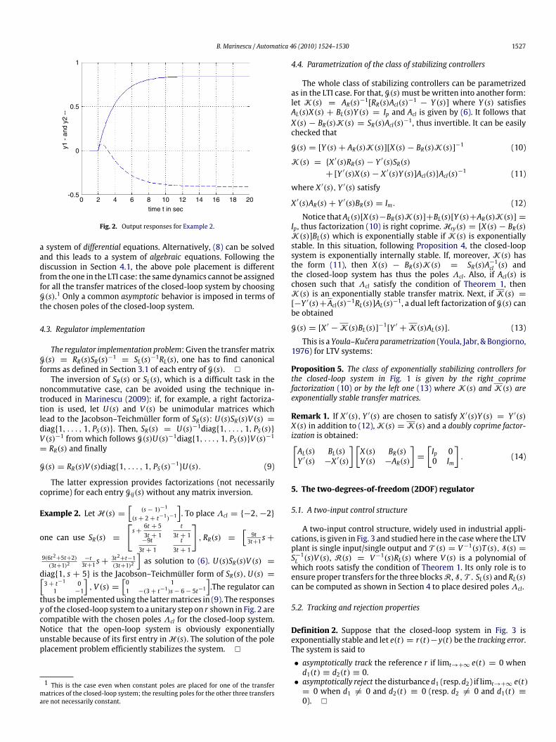
Fig. 2. Output responses for Example 2.

a system of differential equations. Alternatively, (8) can be solvedand this leads to a system of algebraic equations. Following thediscussion in Section 4.1, the above pole placement is differentfrom the one in the LTI case: the samedynamics cannot be assignedfor all the transfer matrices of the closed-loop system by choosingG(s).1 Only a common asymptotic behavior is imposed in terms ofthe chosen poles of the closed-loop system.

4.3. Regulator implementation

The regulator implementation problem: Given the transfermatrixG(s) = RR(s)SR(s)−1 = SL(s)−1RL(s), one has to find canonicalforms as defined in Section 3.1 of each entry of G(s). �The inversion of SR(s) or SL(s), which is a difficult task in the

noncommutative case, can be avoided using the technique in-troduced in Marinescu (2009): if, for example, a right factoriza-tion is used, let U(s) and V (s) be unimodular matrices whichlead to the Jacobson–Teichmüller form of SR(s): U(s)SR(s)V (s) =diag{1, . . . , 1, PS(s)}. Then, SR(s) = U(s)−1diag{1, . . . , 1, PS(s)}V (s)−1 from which follows G(s)U(s)−1diag{1, . . . , 1, PS(s)}V (s)−1= RR(s) and finally

G(s) = RR(s)V (s)diag{1, . . . , 1, PS(s)−1}U(s). (9)

The latter expression provides factorizations (not necessarilycoprime) for each entry Gij(s)without any matrix inversion.

Example 2. LetH(s) =[

(s− 1)−1

(s+ 2+ t−1)−1

]. To place Λcl = {−2,−2}

one can use SR(s) =

[s+

6t + 53t + 1

t3t + 1

−9t3t + 1

t3t + 1

], RR(s) =

[9t3t+1 s+

9(6t2+5t+2)(3t+1)2

−t3t+1 s+

3t2+t−1(3t+1)2

]as solution to (6). U(s)SR(s)V (s) =

diag{1, s + 5} is the Jacobson–Teichmüller form of SR(s),U(s) =[3+ t−1 01 −1

], V (s) =

[0 11 −(3+ t−1)s− 6− 5t−1

].The regulator can

thus be implemented using the lattermatrices in (9). The responsesy of the closed-loop system to a unitary step on r shown in Fig. 2 arecompatible with the chosen poles Λcl for the closed-loop system.Notice that the open-loop system is obviously exponentiallyunstable because of its first entry inH(s). The solution of the poleplacement problem efficiently stabilizes the system. �

1 This is the case even when constant poles are placed for one of the transfermatrices of the closed-loop system; the resulting poles for the other three transfersare not necessarily constant.

4.4. Parametrization of the class of stabilizing controllers

The whole class of stabilizing controllers can be parametrizedas in the LTI case. For that, G(s)must be written into another form:let K(s) = AR(s)−1[RR(s)Acl(s)−1 − Y (s)] where Y (s) satisfiesAL(s)X(s) + BL(s)Y (s) = Ip and Acl is given by (6). It follows thatX(s) − BR(s)K(s) = SR(s)Acl(s)−1, thus invertible. It can be easilychecked that

G(s) = [Y (s)+ AR(s)K(s)][X(s)− BR(s)K(s)]−1 (10)

K(s) = {X ′(s)RR(s)− Y ′(s)SR(s)+ [Y ′(s)X(s)− X ′(s)Y (s)]Acl(s)}Acl(s)−1 (11)

where X ′(s), Y ′(s) satisfy

X ′(s)AR(s)+ Y ′(s)BR(s) = Im. (12)

Notice that AL(s)[X(s)−BR(s)K(s)]+BL(s)[Y (s)+AR(s)K(s)] =Ip, thus factorization (10) is right coprime.Hry(s) = [X(s) − BR(s)K(s)]BL(s) which is exponentially stable if K(s) is exponentiallystable. In this situation, following Proposition 4, the closed-loopsystem is exponentially internally stable. If, moreover, K(s) hasthe form (11), then X(s) − BR(s)K(s) = SR(s)A−1cl (s) andthe closed-loop system has thus the poles Λcl. Also, if Acl(s) ischosen such that Λcl satisfy the condition of Theorem 1, thenK(s) is an exponentially stable transfer matrix. Next, if K(s) =[−Y ′(s)+Acl(s)−1RL(s)]AL(s)−1, a dual left factorization of G(s) canbe obtained

G(s) = [X ′ −K(s)BL(s)]−1[Y ′ +K(s)AL(s)]. (13)

This is a Youla–Kučera parametrization (Youla, Jabr, & Bongiorno,1976) for LTV systems:

Proposition 5. The class of exponentially stabilizing controllers forthe closed-loop system in Fig. 1 is given by the right coprimefactorization (10) or by the left one (13) where K(s) and K(s) areexponentially stable transfer matrices.

Remark 1. If X ′(s), Y ′(s) are chosen to satisfy X ′(s)Y (s) = Y ′(s)X(s) in addition to (12),K(s) = K(s) and a doubly coprime factor-ization is obtained:[AL(s) BL(s)Y ′(s) −X ′(s)

] [X(s) BR(s)Y (s) −AR(s)

]=

[Ip 00 Im

]. (14)

5. The two-degrees-of-freedom (2DOF) regulator

5.1. A two-input control structure

A two-input control structure, widely used in industrial appli-cations, is given in Fig. 3 and studied here in the casewhere the LTVplant is single input/single output and T (s) = V−1(s)T (s), S(s) =S−1L (s)V (s), R(s) = V−1(s)RL(s) where V (s) is a polynomial ofwhich roots satisfy the condition of Theorem 1. Its only role is toensure proper transfers for the three blocksR,S, T . SL(s) andRL(s)can be computed as shown in Section 4 to place desired polesΛcl.

5.2. Tracking and rejection properties

Definition 2. Suppose that the closed-loop system in Fig. 3 isexponentially stable and let e(t) = r(t)−y(t) be the tracking error.The system is said to• asymptotically track the reference r if limt→+∞ e(t) = 0 whend1(t) ≡ d2(t) ≡ 0.• asymptotically reject the disturbanced1 (resp. d2) if limt→+∞ e(t)= 0 when d1 6= 0 and d2(t) ≡ 0 (resp. d2 6= 0 and d1(t) ≡0). �

1528 B. Marinescu / Automatica 46 (2010) 1524–1530

Fig. 3. 2DOF controller.

Proposition 6. Consider an asymptotically stable 2DOF closed-loopsystem as in Fig. 3 with the notations of Section 4.

• a constant reference r is asymptotically tracked if

Acl(0) = (BRT )(0) (15)

where Acl(s) and BR(s) are left coprime polynomials such that

Acl(s)BR(s) = BR(s)Acl(s). (16)

• the aforementioned system asymptotically rejects constant inputdisturbances d1 = const if

SL(0) = 0 or BR(0SL(0)) = 0 (17)

where BR(s) and Acl(s) are left coprime polynomials whichsatisfy (16).• the aforementioned system asymptotically rejects constant outputdisturbances d2 = const if

AL(0) = 0 or SR(0AL(0)) = 0 (18)

where SR(s) and Acl(s) are left coprime polynomials such thatAcl(s)SR(s) = SR(s)Acl(s).

Proof. It follows using the product formula (3). �

Following Proposition 6, T (s) can be chosen to ensure asymp-totic tracking performance for a givenAcl(s).When the feedforwardterm is not used in the 2DOF structure, i.e., when T (s) = 1, condi-tion (15) reduces to

Acl(0) = BR(0) (19)

and thus the asymptotic tracking can no longer be ensured inde-pendent from the pole placement problem for which constraint(19) must be taken into account in this case. Notice that the situa-tion is different from the LTI case where the condition SL(0) = 0,which means that the controller in the direct chain of the closed-loop must have an integral effect, is necessary and sufficient forasymptotic rejection of constant input disturbances. In the LTVcase it is only a sufficient condition. The same holds for the rejec-tion of d1.

5.3. Application to the control of a variable flux DC motor

Consider a separated excitation variable flux DC motor. Thetransfer function from the rotor voltage Vr to the speed ω isH(s) = [s2 + α1(t)s + α0(t)]−1β(t) where α0(t) =

fRrLr J+

KmKefLr J

Φ(t)2, α1(t) =fJ −

Φ(t)Φ(t) , β(t) =

KmΦ(t)JLr. If the variation in

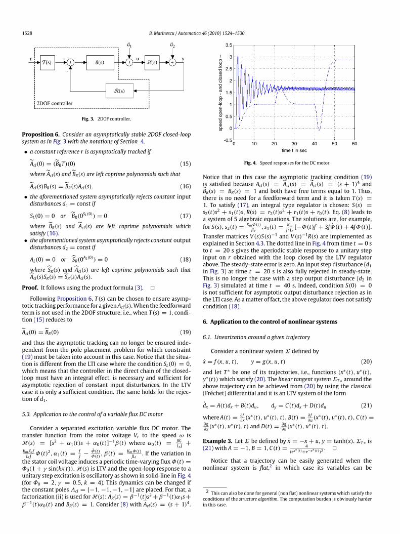
the stator coil voltage induces a periodic time-varying fluxΦ(t) =Φ0(1 + γ sin(kπ t)),H(s) is LTV and the open-loop response to aunitary step excitation is oscillatory as shown in solid-line in Fig. 4(for Φ0 = 2, γ = 0.5, k = 4). This dynamics can be changed ifthe constant polesΛcl = {−1,−1,−1,−1} are placed. For that, afactorization (ii) is used forH(s): AR(s) = β−1(t)s2+β−1(t)α1s+β−1(t)α0(t) and BR(s) = 1. Consider (8) with Acl(s) = (s + 1)4.

3.5

3

2.5

2

1.5

1

0.5

0

-0.5

spee

d op

en-lo

op -

and

clo

sed

loop

--

0 10 20 30time t in sec

40 50 60

Fig. 4. Speed responses for the DC motor.

Notice that in this case the asymptotic tracking condition (19)is satisfied because Acl(s) = Acl(s) = Acl(s) = (s + 1)4 andBR(s) = BR(s) = 1 and both have free terms equal to 1. Thus,there is no need for a feedforward term and it is taken T (s) =1. To satisfy (17), an integral type regulator is chosen: S(s) =s2(t)s2 + s1(t)s, R(s) = r2(t)s2 + r1(t)s + r0(t). Eq. (8) leads toa system of 5 algebraic equations. The solutions are, for example,for S(s), s2(t) = KmΦ(t)

JLr, s1(t) = Km

J2Lr[−Φ(t)f + 3JΦ(t)+ 4JΦ(t)].

Transfer matrices V (s)S(s)−1 and V (s)−1R(s) are implemented asexplained in Section 4.3. The dotted line in Fig. 4 from time t = 0 sto t = 20 s gives the aperiodic stable response to a unitary stepinput on r obtained with the loop closed by the LTV regulatorabove. The steady-state error is zero. An input step disturbance (d1in Fig. 3) at time t = 20 s is also fully rejected in steady-state.This is no longer the case with a step output disturbance (d2 inFig. 3) simulated at time t = 40 s. Indeed, condition S(0) = 0is not sufficient for asymptotic output disturbance rejection as inthe LTI case. As amatter of fact, the above regulator does not satisfycondition (18).

6. Application to the control of nonlinear systems

6.1. Linearization around a given trajectory

Consider a nonlinear systemΣ defined by

x = f (x, u, t), y = g(x, u, t) (20)

and let T ∗ be one of its trajectories, i.e., functions (x∗(t), u∗(t),y∗(t))which satisfy (20). The linear tangent systemΣT∗ around theabove trajectory can be achieved from (20) by using the classical(Fréchet) differential and it is an LTV system of the form

dx = A(t)dx + B(t)du, dy = C(t)dx + D(t)du (21)

whereA(t) = ∂ f∂x (x

∗(t), u∗(t), t), B(t) = ∂ f∂u (x

∗(t), u∗(t), t), C(t) =∂g∂x (x

∗(t), u∗(t), t) and D(t) = ∂g∂u (x

∗(t), u∗(t), t).

Example 3. Let Σ be defined by x = −x + u, y = tanh(x). ΣT∗ is(21) with A = −1, B = 1, C(t) = 4

(ex∗(t)+e−x∗(t))2. �

Notice that a trajectory can be easily generated when thenonlinear system is flat,2 in which case its variables can be

2 This can also be done for general (non flat) nonlinear systems which satisfy theconditions of the structure algorithm. The computation burden is obviously harderin this case.

B. Marinescu / Automatica 46 (2010) 1524–1530 1529

written in function of the flat output and a finite number ofits derivatives (see Fliess, Lévine, Martin, & Rouchon, 1995, andrelated references). System of Example 3 is flat with the flat outputy. Indeed, x = 1

2 ln1+y1−y , u = x + x and this can be exploited

to generate (x∗(t), u∗(t)) consistent with a given desired outputy∗(t).

6.2. Trajectory tracking by LTV control

The problem of asymptotic tracking of a desired output trajectory,i.e., limt→+∞(y(t)−y∗(t)) = 0, can be solved by computing an LTVregulator for (21) with the methodology presented in Section 4.

Proposition 7. Let Σ be a nonlinear system, T ∗ one of its trajectories(x∗(t), u∗(t), y∗(t)) and ΣT∗ the linear tangent system around T ∗.Suppose that the uncontrollable modes of ΣT∗, if any, satisfy thecondition of Theorem 1 (i.e., ΣT∗ is exponentially stabilizable). Then,G(s) can be chosen to exponentially stabilize the linear closed-loopsystem in Fig. 1 whereH(s) is the transfer matrix of ΣT∗ and, whenapplied to the nonlinear system Σ , i.e., as in Fig. 1 where H(s) isreplaced by Σ, r is replaced by u∗ and d by −y∗, to provide anasymptotic tracking of the desired output trajectory y∗(t). �

Proof. Let x = f (x, u, t), y = g(x, u, t), where x = x −x∗, u = u − u∗, y = y − y∗, f (x, u, t) = f (x, u, t) −f (x∗, u∗, t), g(x, u, t) = g(x, u, t) − g(x∗, u∗, t) be the variationalsystem of (20) relative to trajectory T ∗. Obviously, (x = 0, u =0, y = 0) is an equilibrium point of the variational system.Moreover, ∂ f

∂x (0, 0, t) =∂ f∂x (x

∗, u∗, t), ∂ f∂u (0, 0, t) =

∂ f∂u (x

∗, u∗, t),∂g∂x (0, 0, t) =

∂g∂x (x

∗, u∗, t), ∂g∂u (0, 0, t) =

∂g∂u (x

∗, u∗, t) and dx =dx, du = du, dy = dy. Thus, the linear tangent ET0 of the variationalsystem around the origin is ΣT∗ given by (21). It follows thatG(s) asymptotically stabilizes also the closed-loop system in Fig. 1where H(s) is the transfer matrix of ET0 . If, moreover, G(s) ischosen such that entries of the state-matrix of the closed-loopsystem are bounded and Lipschitz in a neighboring of the origin,3using Lyapunov’s indirect method, it follows that the origin is anasymptotically stable equilibrium point of the nonlinear closed-loop system and thus limt→+∞(y(t)− y∗(t)) = 0. �

For Example 3, H(s) = [1 − y(t)∗2](s + 1)−1 and a 2DOFregulatorwhich places the poles of the closed-loop system toΛcl ={−1,−1} is S(s) = [1 − y(t)∗2]s, R(s) =

(1− 4 y

∗ y∗

1−y∗2

)s + 1 −

2y∗ y∗−2y∗y∗2+y∗y∗4+y∗−y∗y∗2+2y∗2y∗

1−y∗2− 2(1 + y∗2). When trajectory

y∗(t) = 0.9(1 − e−t) is used (i.e., if a first order type responseis desired), the response y of the nonlinear closed-loop systemwith zero initial conditions is given in Fig. 5 from t = 0 s tot = 20 s. A unitary step input disturbance applied at time t = 20 sis also rejectedwith good transients andwithout steady-state errorbecause condition (17) is satisfied (S(0) = 0). The control abovestabilizes the nonlinear closed-loop system only locally aroundtrajectory T ∗ ofΣ . The domain of validity of such a control dependson the application (i.e., on the nature of Σ) and it is difficult toestimate (this means to investigate the convergence properties ofthe closed-loop system as defined in Pavlov, van der Wouw, andNijmeijer (2007) and related references). In general, the closed-loop system can be driven around the linearization trajectory byincluding a supplementary reference signal, i.e. r for the 2DOFregulator in Fig. 3. For Example 3, in Fig. 5 it is shown from timet = 40 s to t = 60 s the response y to a step of magnitude 0.09 onreference r .

3 Notice that this condition is trivially satisfied if the state-matrix has constantentries, i.e., if constant poles are placed for the closed-loop system.

outp

ut y

0 10 20 30time t

40 50 60

1

0.8

0.9

0.7

0.6

0.5

0.4

0.3

0.2

0.1

0

Fig. 5. Output response for Example 3.

Remark 2. The trajectory tracking presented above is a particularcase of the general output regulation problem for nonlinearsystems (see Byrnes & Isidori, 1998, and related references). Here,the model of the exosystem coincides with the model of the plant(20). �

7. Concluding remarks

The output feedback pole placement is treated in an input–output algebraic framework for LTV systems. The solutions coverthe cases of: systems with poles in a larger field than the one ofthe coefficients of the system, multi input–multi output systems,systems with non trivial zeros (not only transfer matrices withnumerators reduced to constant gains as in Zhu et al. (1990)). Thestability of the closed-loop system is assessed as in the LTI case(Proposition 4 and Corollary 1). It is also clarified what dynamicscan be assigned by LTV pole placement in comparison to theLTI case. Also, the algorithms are constructive from the practicalimplementation point of view.Beyond the framework of LTV systems, the results presented

here open the way to the control of general (i.e., not necessarilyflat systems or flat systems for which the flat output does not co-incide with the output to be controlled) nonlinear systems usingtheir linearizations around an a priori given trajectory (Proposi-tion 7). A direct application is for the gain scheduling control. Indeed,when the scheduling is done on a reference trajectory, the LTV ap-proach presented above allows a direct solution. The stability of theclosed-loop system is better assessed and the usual hypothesis ofslow varying input and scheduling variable under which the refer-ence trajectory scheduling was previously done can be skipped.

References

Bourlès, H. (2005). Structural properties of discrete and continuous linear time-varying systems: a unified approach. In F. Lamnabhi-Lagarrigue, A. Loría, & E.Panteley (Eds.), Advanced topics in control systems theory (pp. 225–280) Springer(Chapter 6).

Bourlès, H., & Fliess, M. (1997). Finite poles and zeros of linear systems: an intrinsicapproach. International Journal of Control, 68, 897–922.

Byrnes, C. I., & Isidori, A. (1998). Output regulation for nonlinear systems: anoverview. In Proc. of the 37th conference on decision and control. Tampa, Florida,USA.

Cohn, P. M. (1985). Free rings and their relations. Academic Press.Emre, E., Tai, H. M., & Seo, J. H. (1990). Transfer matrices, realization, andcontrol of continuous-time linear time-varying systems via polynomial fractionrepresentations. Linear Algebra and its Applications, 141, 79–104.

Fliess, M. (1990). Une interprétation algébrique de la transformation de Laplace etdes matrices de transfert. Linear Algebra and its Applications, 203, 429–443.

Fliess,M., Lévine, J., Martin, P., & Rouchon, P. (1995). Flatness and defect of nonlinearsystems: introductory theory and examples. International Journal of Control,61(6), 1327–1361.

Guglielmi, M. (2002). Systèmes linéaires variables dans le temps. In Ph. de Larminat(Ed.)., Commande des systèmes linéaires (pp. 271–284) Paris: Lavoisier (Chapter8).

1530 B. Marinescu / Automatica 46 (2010) 1524–1530

Kamen, E.W., Khargonekar, P. P., & Poolla, K. R. (1985). A transfer-function approachto linear time-varying discrete-time systems. SIAM Journal on Control andOptimization, 23(4).

Malgrange, B. (1962–1963). Systèmes différentiels à coefficients constants.Séminaire Bourbaki, 246, 1–11.

Marinescu, B. (2009).Model-matching anddecoupling for continuous- anddiscrete-time linear time-varying systems. International Journal of Control, 82(6),1018–1028.

Marinescu, B., & Bourlès, H. (2009). An intrinsic algebraic setting for poles and zerosof linear time-varying systems. Systems and Control Letters, 58, 248–253.

Pavlov, A., van der Wouw, N., & Nijmeijer, H. (2007). Global nonlinear outputregulation: convergence-based controller design. Automatica, 43(3), 456–463.

Poola, K., & Khargonekar, P. (1987). Stabilizability and stable-proper factorizationsfor linear time-varying systems. SIAM Journal on Control and Optimization, 25(3),723–736.

Rotella, F. (2003). Systèmes linéaires non stationnaires. Techniques de l’ingénieur,traité informatique industrielle, no. R7185 (pp. 1–16).

Valášek, M., & Olgac, N. (1999). Pole placement for linear time-varying non-lexicographically fixed MIMO systems. Automatica, 35, 101–108.

Youla, D. C., Jabr, H. A., & Bongiorno, J. (1976). Modern Wiener–Hopf designof optimal controllers—part II: the multivariable case. IEEE Transactions onAutomatic Control, AC-21(3).

Zhu, J., Johnson, C. D., Thompson, P., & Wendt, R. (1990). Stabilization of time-varying linear systems using a new time-varying eigenvalue assignementtechnique. In Proceedings IEEE southeastcon (pp. 212–218).

Bogdan Marinescuwas born in 1969 in Bucharest, Roma-nia. He obtained his Engineering Degree from the Poly-technical Institute of Bucharest in 1992 and the M.Sc. andPh.D. fromUniversité Paris Sud-Orsay (France) in 1994 and1997 respectively. He is currently research engineer at theFrench Transmission SystemOperator (RTE) and AssociateProfessor at EcoleNormale Supérieure de Cachan.Hismainfields of interest are the theory and applications of linearsystems, robust control and power systems engineering.