outline informatique visuelle - vision par ordinateur ... · informatique visuelle - vision par...

Informatique visuelle - Vision par ordinateur

Motion and tracking

Elise Arnaud

thanks to E. Memin, A. Boucher, Y. Ukrainitz, B. Sarel, K. Grauman, S. Lazebnik, B. Leibe for slide

inspiration.

Elise Arnaud M2P UFR IMA

Outline

Introduction

General framework: from 3D to 2D

Problems

Motion detection

Motion field estimation

Tracking


Outline

Introduction


Problems

Motion detection


Tracking


Framework: multi-image analysis

Cameras :

sensors of variable geometry, of low price and easy to use

but : useful information is difficult to extract from the images

Perception et understanding of the environnement from images:

one image : 2D projection of the 3D world ⇒ incomplete andstatic information

several images : richer information on 3D and/or temporalthanks to spatial and/or temporal redundancy

using several images ⇒ match up information


Framework: multi-image analysis

Cameras :

sensors of variable geometry, of low price and easy to use

but : useful information is difficult to extract from the images

Perception et understanding of the environnement from images:

one image : 2D projection of the 3D world ⇒ incomplete andstatic information

several images : richer information on 3D and/or temporalthanks to spatial and/or temporal redundancy

using several images ⇒ match up information


Human vs computer

Visual system : images and a priori knowledge (size, behaviour,spatial organization, object dynamics, etc.)

one eye (+ a priori)

no motion vague qualitative info on the 3D scenehead motion more reliable info on the 3D scenescene motion perception of apparent motion and info on the 3D scene

two eyes (+ a priori)

no motion good perception of relative depthshead motion even more reliable info on the 3D scenescene motion 3D perception of motion and structures


Human vs computer







Human vs computer







Human vs computer

Computer vision : image sequences and very few a priori ...

motion may be due to :

movement in scene

movement of camera (ego motion)


Use of motion

Analyzing motion can be useful for

estimating 3D structure

Segmentation of moving objects

tracking objects, features over time

Motion is a very important feature !

see videos


Applications

medical imagery (echography, endoscopy)

robotics (to avoid obstacles, environment perception)

satelitte imagery (meteorology, oceanography, remotedetection)

road trafic (surveillance, driving help )

human motion analysis (hmi, sport gesture)

image synthesis, animation (e.g. augmented reality)

codage and video compression

military applications

tool for experimental sciences (fluid mechanics, biology, etc.)

...


Outline

Introduction


Problems

Motion detection


Tracking


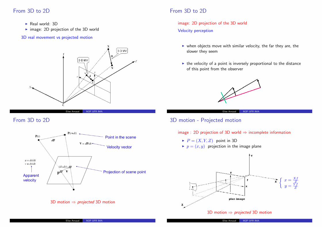
From 3D to 2D

Real world: 3D image: 2D projection of the 3D world

3D real movement vs projected motion


From 3D to 2D

image: 2D projection of the 3D world

Velocity perception

when objects move with similar velocity, the far they are, theslower they seem

the velocity of a point is inversely proportional to the distanceof this point from the observer


From 3D to 2D

3D motion ⇒ projected 3D motion


3D motion - Projected motion

image : 2D projection of 3D world ⇒ incomplete information

P = (X,Y, Z) point in 3D p = (x, y) projection in the image plane

x = Xf

Z

y = Y fZ

3D motion ⇒ projected 3D motion


3D motion - Projected motionP = (X,Y, Z) point at the surface of a solide whose 3D motion is:

.X.Y.Z

=

ABC

+

Ω1

Ω2

Ω3

∧

XYZ



v = (u, v) motion of the projected point p = (x, y) (case f = 1)

x = Xf

Z

y = Y fZ

⇒

u =.x=

.XZ−

.ZX

Z2

v =.y=

.Y Z−

.ZY

Z2

u =

.x= A

Z + Ω2 − Ω3y − xCZ − Ω1xy + Ω2x2

v =.y= B

Z + Ω1 + Ω3x− yCZ + Ω2xy − Ω1y2

From 3D motion, we can calculate the projected motion.

reciprocal rarely true ... (⇒ use several cameras !).



Few exemples, fixed scene (no moving object)

Pure translation of the camera along the X axis: A = 0

⇒ 2D translation: apparent velocity horizontal, and module inverselyproportionnal to the depth

Pure translation of the camera along the Z axis: C = 0

⇒ 2D divergence: zoom on the image

Pure rotation of the camera around the Z axis: Ω3 = 0

⇒ 2D rotation

Pure rotation of the camera around the X axis: Ω1 = 0

⇒ 2D translation









⇒ 2D rotation


⇒ 2D translation









⇒ 2D rotation


⇒ 2D translation









⇒ 2D rotation


⇒ 2D translation









⇒ 2D rotation


⇒ 2D translation


Projected motion - apparent motion

projected motion : projection in the image plane of the 3Dmotion of visible elements in the scene

apparent motion : 2D motion ”seen” in an image sequencethanks to spatio-temporal variation of the luminance

famous example: rotation of a uniform sphere

Apparent motion = Projected motion !


Outline

Introduction


Problems

Motion detection


Tracking


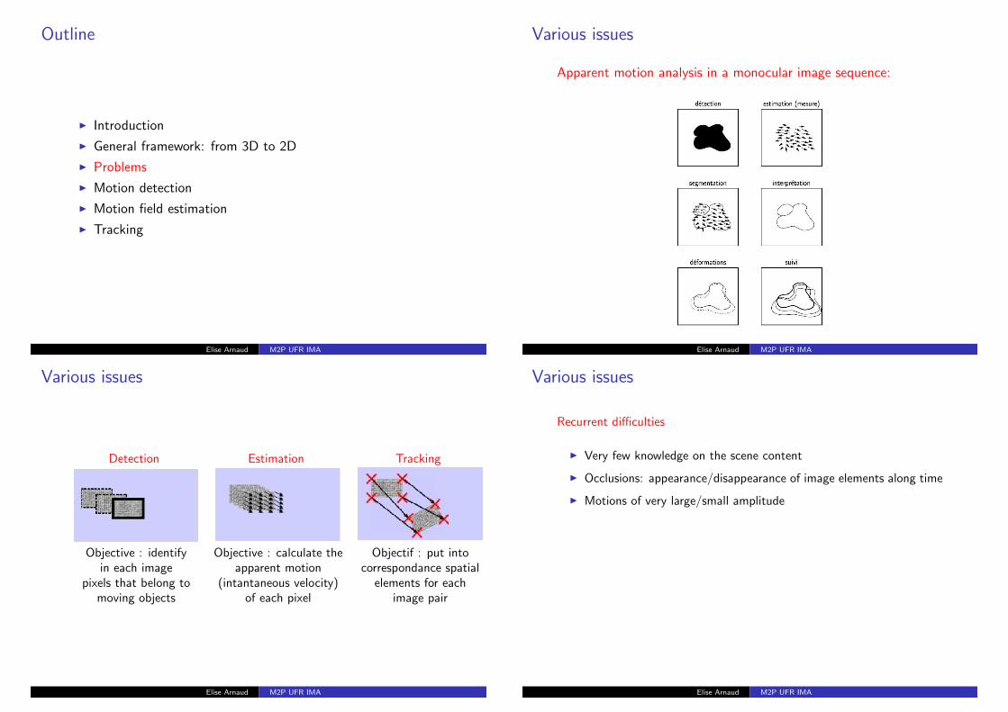
Various issues

Apparent motion analysis in a monocular image sequence:


Various issues

Detection Estimation Tracking

Objective : identify Objective : calculate the Objectif : put intoin each image apparent motion correspondance spatial

pixels that belong to (intantaneous velocity) elements for eachmoving objects of each pixel image pair


Various issues

Recurrent difficulties

Very few knowledge on the scene content

Occlusions: appearance/disappearance of image elements along time

Motions of very large/small amplitude

Assumption

1. Geometric / photometric invariants

interaction models data - unknows

2. Use of spatial / temporal context

a priori models on unknowns


Various issues

Recurrent difficulties

Very few knowledge on the scene content

Occlusions: appearance/disappearance of image elements along time

Motions of very large/small amplitude

Assumption

1. Geometric / photometric invariants

interaction models data - unknows

2. Use of spatial / temporal context

a priori models on unknowns


Outline

Introduction


Problems

Motion detection


Tracking


Motion detection

goal: detect moving objects using a cameraProblem: distringuish changes in the image due to motion

Applications

road traffic control

surveillance

augmented reality

tracking

etc.


Motion detection

Assumptions

fixed camera

fixed illumination condition

⇒ significative changes only due to motion

no a priori knowledge on object dynamic

no a priori knowledge on object nature

What to solve ?

Detection of significative temporal changes of the luminancefunction.

Done by comparing successive images or by comparing with areference image


Motion detection

Assumptions

fixed camera

fixed illumination condition

⇒ significative changes only due to motion

no a priori knowledge on object dynamic

no a priori knowledge on object nature

What to solve ?

Detection of significative temporal changes of the luminancefunction.

Done by comparing successive images or by comparing with areference image


Motion detection

3 categories of changes

background hidden by the moving object

background made visible by the moving object

sliding of the object on it-self (pbl if uniform object)


Motion detection

Few naıve ideas ( but that may be efficient ...)

inter-image difference:

In each pixel s, threshold the inter-image difference

|I2(s)− I1(s)|?> threshold

yes means a significative change

Mean inter-image difference

Let us consider a window W(s) around s of size n× n

r∈W(s) |I2(r)− I1(r)|n× n

?> threshold


Motion detection

Few naıve ideas ( but that may be efficient ...)

inter-image difference:

In each pixel s, threshold the inter-image difference

|I2(s)− I1(s)|?> threshold

yes means a significative change

Mean inter-image difference

Let us consider a window W(s) around s of size n× n

r∈W(s) |I2(r)− I1(r)|n× n

?> threshold


Motion detection


Motion detection


Motion detection - classication of changes

Keep one mask of changes using logical operations

but difficulties due tonoise and uniform objects


Motion detection - results


Motion detection - applications


Outline

Introduction


Problems

Motion detection


Tracking


Motion estimationDense estimation of the apparent motion field

apparent motion field = optical flow associate to each pixel s = (x, y) a motion vector

v(s) = (u, v) that represents its instantaneous apparentvelocity.

Study the variations of the luminance function I(x, y, t)


Motion estimation

Example of optical flow


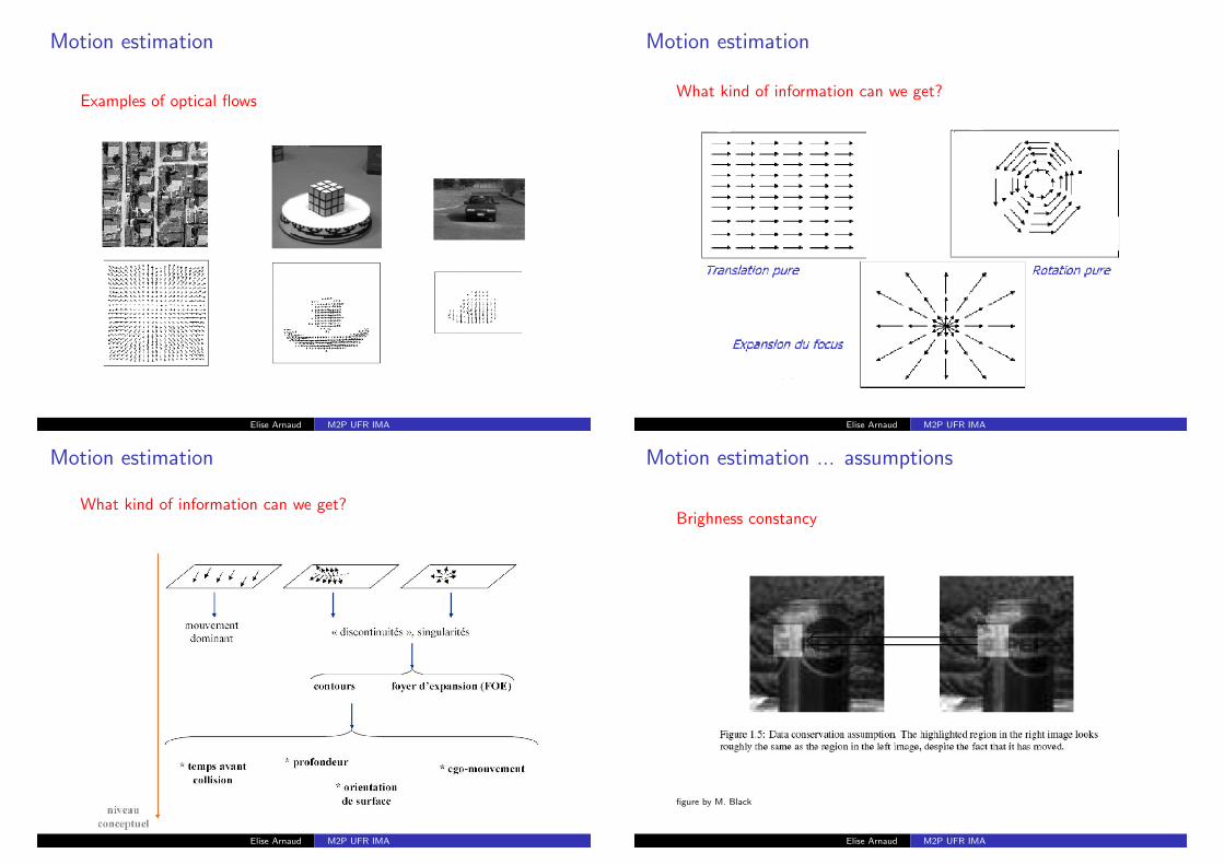
Motion estimation

Examples of optical flows


Motion estimation

What kind of information can we get?


Motion estimation

What kind of information can we get?


Motion estimation ... assumptions

Brighness constancy

figure by M. Black



Spatial coherence

figure by M. Black



To recover optical flow, we need some assumptions

Brightness constancy – In spite of motion, imagemeasurement in small region will remain the same

Spatial coherence – Assume nearby points belong to the samesurface, thus have similar motions, so estimated motionshould vary smoothly

Difficulties

illumination changes

occlusions

specularity, transparency






Difficulties


occlusions







Difficulties


occlusions







Difficulties


occlusions



Motion estimation

+ contextual information

1. ∀s, I2(s+ v(s)) = I1(s)

⇒ Block-matching approaches

2. dI(x,y,t)dt = 0

⇒ Differential approaches


block-matching methods

W(s) is a window centered in s

Goal : Find v(s) that maximises the similarity between I1 inW(s) and I2 in W(s+ v(s))


block-matching methods

similarity measures

sum of absolute values

r∈W(s)

|I2(r + v)− I1(r)|

sum squared differences

r∈W(s)

(I2(r + v)− I1(r))2

correlation

r∈W(s)

I2(r + v).I1(r)


differential approaches

dI(x, y, t)

dt= 0

dI(x, y, t)

dt=

∂I

∂x

dx

dt+

∂I

∂y

dy

dt+

∂I

∂t= 0

∂I∂x ; ∂I

∂y : spatial image gradients: how image varies in x or ydirection for fixed time

∂I∂t : temporal image derivative: how image varies in time forfixed position

dxdt = u, dx

dt = v, temporal derivatives, i.e. velocitycomponents: rate of change in x and y



dI(x, y, t)

dt= 0

dI(x, y, t)

dt=

∂I

∂x

dx

dt+

∂I

∂y

dy

dt+

∂I

∂t= 0

∂I∂x ; ∂I



dxdt = u, dx




dI(x, y, t)

dt= 0

dI(x, y, t)

dt=

∂I

∂x

dx

dt+

∂I

∂y

dy

dt+

∂I

∂t= 0

∂I∂x ; ∂I



dxdt = u, dx




dI(x, y, t)

dt= 0

dI(x, y, t)

dt=

∂I

∂x

dx

dt+

∂I

∂y

dy

dt+

∂I

∂t= 0

∂I∂x ; ∂I



dxdt = u, dx




dI(x, y, t)

dt= 0

dI(x, y, t)

dt=

∂I

∂x

dx

dt+

∂I

∂y

dy

dt+

∂I

∂t= 0

∂I∂x ; ∂I



dxdt = u, dx




dI(x, y, t)

dt= 0

dI(x, y, t)

dt=

∂I

∂x

dx

dt+

∂I

∂y

dy

dt+

∂I

∂t= 0

rewritten as∂I

∂t+∇IT .v = 0

where v = (u, v) is the unknown velocity



∂I

∂t+∇IT .v = 0

where v = (u, v) is the unknown velocity

one equation, two unknowns .... infinitely many solutions !



∂I

∂t+∇IT .v = 0

where v = (u, v) is the unknow velocity

one equation, two unknowns .... infinitely many solutions !

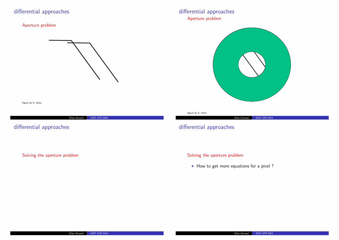
Aperture problem: We can only compute projection of thetrue flow vector in the direction of the image gradient that is,in the direction normal to the image edges

Flow component in gradient direction determined flow component parallel to edge unknown



Aperture problem

figure by S. Seitz


differential approachesAperture problem

figure by S. Seitz



Solving the aperture problem

How to get more equations for a pixel ?

Basic idea: impose additional constraints

Spatial coherence constraint: pretend the pixel’s neighborshave the same v = (u, v)

Lucas Kanade approach























differential approachesSolving the aperture problem - Lucas Kanade approach

Spatial coherence constraint: pretend the pixel’s neighborshave the same (u, v)

If we use a 5× 5 window, that gives us 25 equation per pixels

∂I

∂t+∇IT .[u v] = 0

Ix(p1) Iy(p1)Ix(p2) Iy(p2)

......

Ix(p25) Iy(p25)

uv

= −

It(p1)It(p2)

...It(p25)

B. Lucas and T. Kanade. An iterative image registration technique with an application to stereo vision. In

Proceedings of the International Joint Conference on Artificial Intelligence, pp. 674-679, 1981.


differential approachesSolving the aperture problem - Lucas Kanade approach

least squares problem

Ix(p1) Iy(p1)Ix(p2) Iy(p2)

......

Ix(p25) Iy(p25)

uv

= −

It(p1)It(p2)

...It(p25)

⇔ A

25×2

v = b25×1

Minimum least squares solution given by solution of

ATA 2×2

v = AT b2×1



Solving the aperture problem - Lucas Kanade approach

ATA 2×2

v = AT b2×1

IxIx

IxIy

IyIx

IyIy

uv

= −

IxItIyIt

The summations are over all pixels in the K ×K window When is this solvable

ATA should be invertible ATA should be well-conditioned ATA is equal to matrix M in the Harris detector ...




M = ATA

The eigenvectors and eigenvalues of M relate to edgedirection and magnitude.

The eigenvector associated with the larger eigenvalue pointsin the direction of fastest intensity change.

The other eigenvector is orthogonal to it




1. Estimate at each pixel using one iteration of Lucas andKanade estimation.

2. Warp one image toward the other using the estimated flowfield. (Easier said than done)

3. Refine estimate by repeating the process.

method that can not be applied to all points ... how to get adense map ?

computationally expensive


differential approachesSolving the aperture problem



most common is to assume that the flow field is smoothlocally

Ex. Look for v that minimizes:

x

∂I

∂t(x) +∇IT (x).v(x)

2

Brightness constency

+λ||∇u(x)||2 + ||∇v(x)||2

Spatial coherence

B.K.P. Horn and B.G. Schunck, ”Determining optical flow.” Artificial Intelligence, vol 17, pp 185-203, 1981.


differential approachesone additional ingredient

differential approaches are based on linearization valid only for small displacement ... so how can we do if we have large displacement ? multi-scale approach


differential approachesone additional ingredient


Optical flow - example of applications

Calculation of various depth layers in the image



Mosaicking



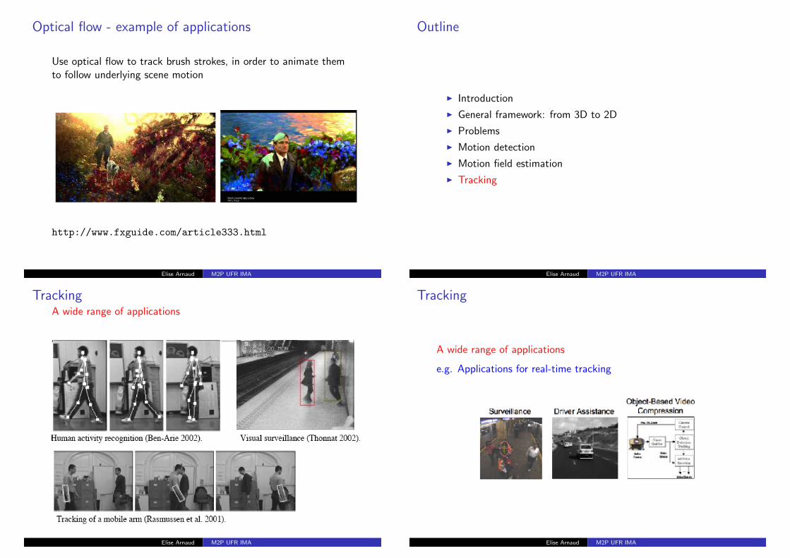
Use optical flow to track brush strokes, in order to animate themto follow underlying scene motion

http://www.fxguide.com/article333.html


Outline

Introduction


Problems

Motion detection


Tracking


TrackingA wide range of applications


Tracking

A wide range of applications

e.g. Applications for real-time tracking


Tracking - difficulties


Tracking


Tracking

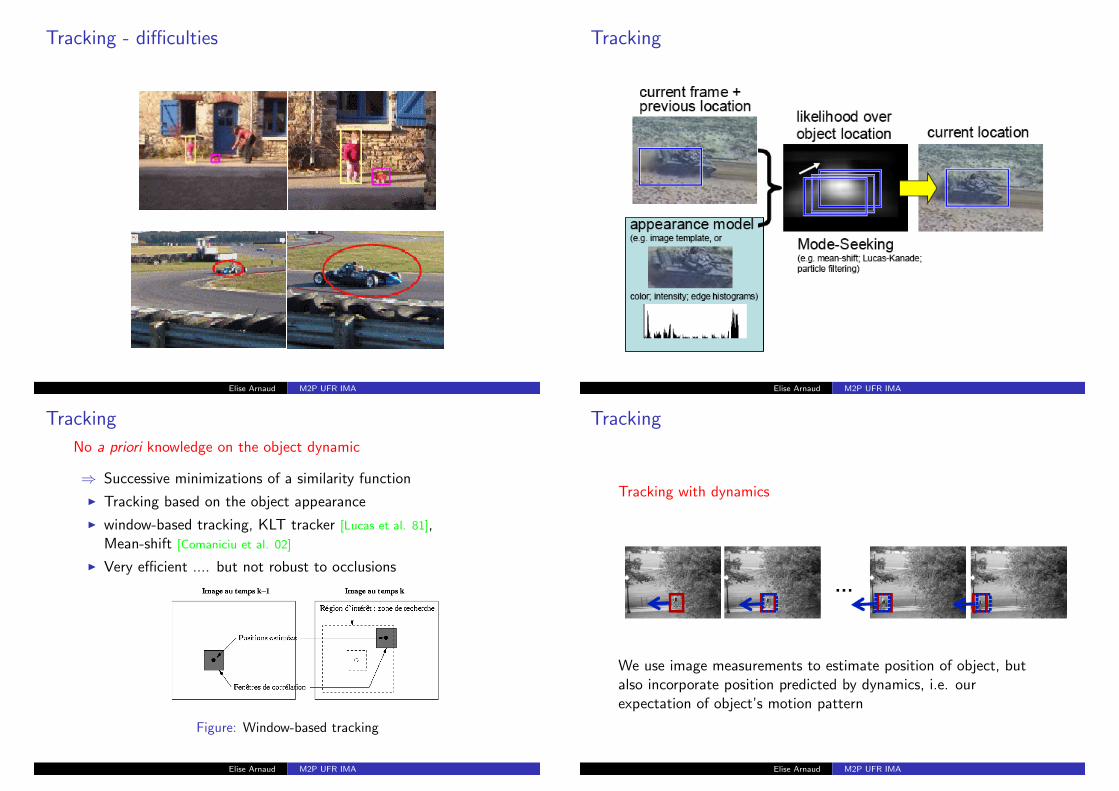
No a priori knowledge on the object dynamic

⇒ Successive minimizations of a similarity function

Tracking based on the object appearance

window-based tracking, KLT tracker [Lucas et al. 81],Mean-shift [Comaniciu et al. 02]

Very efficient .... but not robust to occlusions

Figure: Window-based tracking


Tracking

Tracking with dynamics

We use image measurements to estimate position of object, butalso incorporate position predicted by dynamics, i.e. ourexpectation of object’s motion pattern



Have a model of expected motion

Given that, predict where objects will occur in next frame,even before seeing the image

Intents do less work looking for the object: restrict search improve estimates since measurement noise tempered by

trajectory smoothness be robust to occlusions



Have a model of expected motion

Given that, predict where objects will occur in next frame,even before seeing the image

Intents do less work looking for the object: restrict search improve estimates since measurement noise tempered by

trajectory smoothness be robust to occlusions


Tracking with dynamics - general assumptions

Expect motion to be continuous, so we can predict onprevious trajectories

camera is not moving instantly from viewpoint to viewpoint objects do not disappear and reappear in different places in the

scene gradual change in pose between camera and scene

able to model the motion

Bayesian filter


outline informatique visuelle - vision par ordinateur ... · informatique visuelle - vision par...

Documents