Outline• (HIBP) diagnostics in the MST-RFP• Relationship of equilibrium potential measurements

with plasma parameters• Simulation with a finite-sized beam model

Description of the model and an example Applications of the finite-sized beam model

• Simulation of detector currents during a sawtooth cycle• Instrumental error analysis• Numerical experiments

• Sources of uncertainty in potential measurements Non-ideal fields in the energy analyzer Secondary electron emission Entrance angle of detected ions in the analyzer Plasma and UV loading Plasma density gradients Beam attenuation

• Conclusion

MST HIBP

• Cross over sweeps to accommodate small ports• Magnetic suppression structures to reduce plasma loading• Magnetic field largely plasma produced (reconstructed from MSTFit)

ion beam Na+ or K+

Na+ enters plasma

magetic field separates Na++ from Na+

Na++ detected in the energy analyzer

Na++ in the split plate detector

Heavy Ion Beam Probing

• Quantities measured in MST Potential Potential fluctuations Density fluctuations

Secondary Ion Currents

• Sources of uncertainty in potential measurements variations in beam attenuation factors Fp, Fs

variations in sample volume length lsv

Gradient in local electron density ne

C1

C3

C2

C4

Beam image on the split plates of the energy analyzer

)(0 svesvionspp

ss rnlFFI

q

qkI

Measurement of Electrostatic Potential

• Potential measurement is sensitive to Entrance angles of ions into the analyzer Calibration of the analyzer (XD, YD, d, w) Accuracy of analyzer voltages and detected current

signals

id WWe

gLU

LUIIa V

ii

iiFGV

}),(),({2

22 cossin4

tan),(

I

DIDI d

YXG

22 cossin8

)tancos(sin),(

I

IaaI d

wF

Discharges in MST

5 10 15 20 25200

400

I p (k

A)

S tandard Discharge

5 10 15 20 250.5

1

1.5

ne

(10

13cm

-3)

5 10 15 20 25-1

-0.5

0

F

5 10 15 20 250

50

v 6(k

m/s)

5 10 15 20 250

10

20

Bp

(Gs)

t(ms)

5 10 15 20 25-20

02040

Vtg

(kV)

t(ms)

5 10 15 20 25200

400

I p (k

A)

PPCD

5 10 15 20 250.5

1

1.5

ne

(10

13cm

-3)

5 10 15 20 25-1

-0.5

0

F

5 10 15 20 250

50

v 6(k

m/s)

5 10 15 20 250

10

20

Bp

(Gs)

t(ms)

5 10 15 20 25-20

02040

Vtg

(kV)

t(ms)

5 10 15 20 25200

400

I p (k

A)

Locked

5 10 15 20 250.5

1

1.5

ne

(10

13cm

-3)

5 10 15 20 25-1

-0.5

0

F

5 10 15 20 250

50v 6

(km/

s)

5 10 15 20 250

10

20

Bp

(Gs)

t(ms)

5 10 15 20 25-20

02040

Vtg

(kV)

t(ms)

HIBP Measurement ConditionsType of discharge Standard Locked PPCD

Current Ip (kA) 350-380 (high Ip)

270-290 (low Ip)

260-290 490-510 (high Ip)

370-400 (low Ip)

Density ne (1013 cm3) 0.8-1.2 (high Ip)

0.6-1.0 (low Ip)

0.5-1.0 0.8-1.2 (high Ip)

0.6-1.1 (low Ip)

Temperature Te(eV) ~ 300 ~ 350 ~<800

Reversal factor F ~ -0.22 0 ~ -1.0

Velocity vm/n=1/6(km/s)

(mode)

20-40 0 20-40(non-locked)0 (locked)

Potential (kV) 1.2-2.1(high Ip)

0.9-1.2(low Ip)

~ 0.5 ~1.0 (non-locked)~0 (locked)

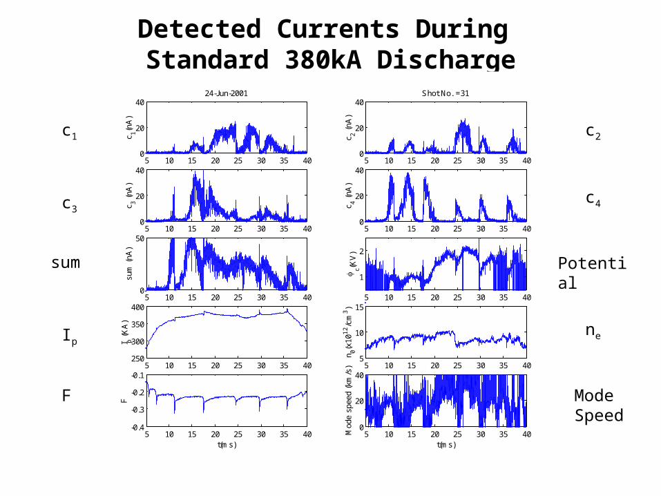
Detected Currents During Standard 380kA Discharge

5 10 15 20 25 30 35 400

20

40

c 1(n

A)

24-Jun-2001

5 10 15 20 25 30 35 400

20

40

c 2 (

nA)

Shot No. =31

5 10 15 20 25 30 35 400

20

40

c 3 (

nA)

5 10 15 20 25 30 35 400

20

40

c 4 (

nA)

5 10 15 20 25 30 35 400

50

sum

(nA

)

5 10 15 20 25 30 35 40

1

2

c(KV

)

5 10 15 20 25 30 35 40250

300

350

400

I p (

KA

)

5 10 15 20 25 30 35 405

10

15

n 0(x

101

2/c

m3)

5 10 15 20 25 30 35 40-0.4

-0.3

-0.2

-0.1

F

t(ms)5 10 15 20 25 30 35 40

0

20

40

Mod

e sp

eed

(km

/s)

t(ms)

c1

c3

c2

c4

sum

Ip

F

Potential

ne

Mode Speed

Sources of Sum Signal Variations

• Variation of sample volume size and location• Variation of beam deflection due to evolution of

magnetic fields• Beam scrape-off• Variation of plasma parameters

Plasma Profile for Standard Discharge

0.2 0.3 0.4 0.5 0.6 0.7 0.8 0.9 10

0.5

1

1.5

2

2.5

r/a

Sc

ale

d p

ote

nti

al (

kV

)

Sawtooth Cycle Potential Variation

18 19 20 21 22 23 24360

380

400I p

(k

A)

18 19 20 21 22 23 24

0.8

1

ne(

10

13c

m-3

)

18 19 20 21 22 23 24

-0.25

-0.2

F

18 19 20 21 22 23 240

40

v 6(k

m/s

)

18 19 20 21 22 23 240.5

2

c(k

V)

18 19 20 21 22 23 240

10

20

Bp(G

s)

t(ms)

Sources of Uncertainty in Potential Measurements

• Variations in plasma characteristics – rotation, density, current, etc.

• Evolution and fluctuations of magnetic and electric fields – affects location, size and orientation of sample volume

• Instrumental Effects Beam scrape-off on apertures, sweep plates, etc. Analyzer geometry Detector noise due to plasma Beam attenuation

Variation of Potential with Plasma Parameters

• Strongest correlation is with mode speed• Only weakly dependent on other parameters

15 20 25 30 35

0.8

0.9

1

1.1

n e ( 1

013cm

-3)

15 20 25 30 35

-0.24

-0.23

-0.22

F

15 20 25 30 35

5

10

15

20B

p(G

s)

15 20 25 30 35

360

370

380

I p(k

A)

v6(km/s)

1

1.5 (kV)

2

15 20 25 30 35

0.2

0.4

0.6

0.8

t saw

too

th

v6(km/s)

Density

Bp

Sawtooth

Cycle Time

Mode Speed

Mode Speed

F

Ip

Finite Beam Simulation

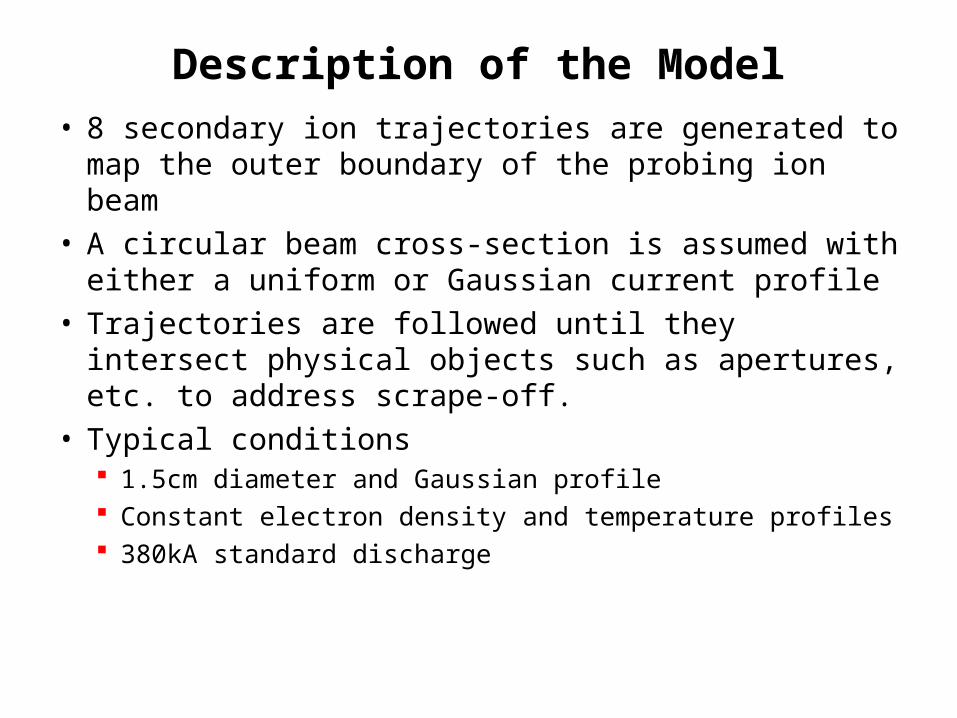
Description of the Model

• 8 secondary ion trajectories are generated to map the outer boundary of the probing ion beam

• A circular beam cross-section is assumed with either a uniform or Gaussian current profile

• Trajectories are followed until they intersect physical objects such as apertures, etc. to address scrape-off.

• Typical conditions 1.5cm diameter and Gaussian profile Constant electron density and temperature profiles 380kA standard discharge

Sample Volume

to centerline of the entrance aperture

to bottom edge of the entrance aperture

to top edge of the entrance aperture

d

sample volume

27 Trajectories are evaluated to represent the secondary ions originating in the sample volume.

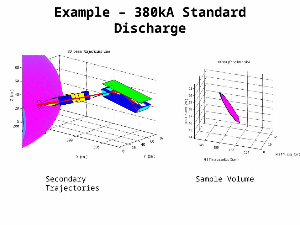
Example – 380kA Standard Discharge

200

250

300

3500

2040

6080

0

20

40

60

80

Y (cm)

3D beam trajectories view

X (cm)

Z (

cm)

148150

152154 8

10

1214

15

16

17

18

19

20

21

MST Y axis (cm)

MST major radius X(cm)

3D sample volume view

MS

T Z

axi

s (c

m)

Secondary Trajectories Sample Volume

Example – 380kA Standard Discharge

-6 -4 -2 0 2 4 6

-5

-4

-3

-2

-1

0

1

2

3

4

5

Outer Exit Port

Y (cm) (toroidal)

Z (

cm)

(rad

ial) magnetic strcture

-15 -10 -5 0 5 10 15-0.5

0

0.5Secondary impact at entrance aperture

Yellow: Effective region

entrance slit length (cm)

entr

ance

slit

wid

th (

cm)

0

2

4

6

8

-8 -6 -4 -2 0 2 4 6 8-0.4

-0.2

0

0.2

0.4

entrance slit length (cm)

entr

ance

slit

wid

th (

cm)

current density profile

Secondary Beams at the Exit Port (Magnetic Aperture)

Secondary Beams at the Analyzer Entrance Aperture

Example – 380kA Standard Discharge

-15 -10 -5 0 5 10 15-1.5

-1

-0.5

0

0.5

1

1.5Secondary impact at detector & current density profile

Yellow: Effective region

detector length (cm)

dete

ctor

wid

th (

cm)

0

1

2

3

4

5

-8 -6 -4 -2 0 2 4 6 8-0.5

0

0.5

detector length (cm)

dete

ctor

wid

th (

cm)

0 10 20 30 40 50 60 70

-25

-20

-15

-10

-5

0

5

10

15

20

25

grids at the energy analyzer ground plates

toro

idal

Y(c

m)

radial X (cm)

ground plate of the analyzer

grids

Secondary Beams at the Analyzer Ground Plane

Secondary Beams at the Analyzer Detector Plates

About half of secondary beam has been scraped-off largely by the sweep plates during the last half phase of a sawtooth cycle

Simulation of Secondary Currents During a 380kA Standard Discharge Sawtooth Cycle

15 20 25 300

20

40

c 1(n

A)

24-Jun-2001

15 20 25 300

20

40

c 2 (

nA)

Shot No. =31

15 20 25 300

20

40c 3

(nA

)

15 20 25 300

20

40

c 4 (

nA)

15 20 25 300

50

sum

(nA

)

15 20 25 30

1

2

c(KV

)

15 20 25 30360

370

380

390

I p (

KA

)

15 20 25 305

10

15

n 0(x

101

2/c

m3)

15 20 25 30-0.4

-0.3

-0.2

-0.1

F

t(ms)15 20 25 30

0

20

40

Mod

e sp

eed

(km

/s)

t(ms)

Typical secondary ion currents on the four plates of the center detector (c1 - c4), sum

signal, and the measured plasma potential c, during a 380 kA standard discharge with

plasma current Ip, electron density n0, reversal factor F and dominant mode velocity.

The vertical lines bracket the sawtooth cycle. A 10 kHz low-pass filter has been applied to the potential and mode velocity to remove the tearing mode fluctuations.

Detected Signals during Sawtooth Cycle

• Agreement between measured and simulated signals• There is significant scrape off • Sample volume position varies by up to 3.5cm

18 20 22 240

10

20

30

c 1

HIBPsimu-insimu-out

18 20 22 240

10

20

30

c 2

18 20 22 240

10

20

30

c 3

t (ms)18 20 22 24

0

10

20

30c 4

t (ms)

18 19 20 21 22 23 24

16

17

18

19

20

21

22

t (ms)

rad

ial p

os

itio

n r

(cm

)

Sample volume position

HIBP: measurement

Simu_in: simulation

Simu_out: simulation after potential adjustment

Potential During Sawtooth Cycle

18 19 20 21 22 23 240

0.2

0.4

0.6

0.8

1

1.2

1.4

1.6

1.8

2

t (ms)

Pot

c (kV

)

HIBPsimu

output pot

calculated currents consistentwith measured HIBP signals?

secondary beam energy = primary beam energy+ potential measured

run finite-sized beam simulation

calculate secondary currents on four slit plates of detector

N

adjust potential

Y

Simu_in

Simu_out

Signal scrape-off does not make a significant contribution to potential measurements because the up-down balance of the beam image on the detector is not affected.

Error Sources: Analyzer Characteristics

-6 -4 -2 0 2 4 62.955

2.96

2.965

2.97

2.975

2.98

2.985

Entrance angle -30( )

Ga

in

center detector (calibrated)bottom detector (calibrated)fitted to equation (XD=654.03 mm, YD=124.96 mm)

-6 -4 -2 0 2 4 60.012

0.014

0.016

0.018

0.02

0.022

0.024

Entrance angle -30( )

F

center detector (calibrated)bottom detector (calibrated)fitted to equation (slit width = 2.4 mm)

Agreement between ideal and measured analyzer characteristics is excellent, but not perfect. Shown are characteristics for both bottom and center detectors. Non-ideal characteristics are typically non-uniform electric fields and slight variations in dimensions. G is more critical to potential measurements than F.

Error Sources: Analyzer Entrance Angle

• The variations of entrance angle are 0.45 ( )and 2.6 ()• The potential uncertainty due to variations of G and F are 0.095 kV.• Errors from simulation (due to scrape off and angles) 0.06 kV.

17 18 19 20 21 22 23 24 2529.8

30

30.2

30.4

30.6

in-p

lan

e a

ng

le

()

17 18 19 20 21 22 23 24 250

1

2

3

ou

t-o

f-p

lan

e a

ng

le

()

t (ms)

17 18 19 20 21 22 23 24 2571.1

71.15

71.2

71.25

71.3

71.35

t (ms)

2*V

a*G

ain

17 18 19 20 21 22 23 24 250.62

0.64

0.66

0.68

t (ms)

2*V

a*F

entrance angle of beam in radial direction and in toroidal direction

Potential variation due to the variation of beam angle

Error Sources: Density Gradient

The Electron density profile obtained from MSTFit over the sawtooth cycle during a typical 380 kA standard discharge.

The thick lines along the density profiles show the simulated HIBP sample volume length when projected onto the horizontal axis.

The potential uncertainty caused by the plasma density gradient in the sample volume is small ( < 0.01 kV ) in the interior of the plasma during a high current standard discharge, and becomes significant (0.05 - 0.11 kV) when the sample volume is moving to the outer area of the plasma.

Summary of Error SourcesSource Uncertainties Potential Uncertainty (V)

Calibration of F Measurement of entrance aperture width

< 54

Beam angle, position and beam scrape-off

Variation of beam entrance angles< 0.45, < 2.6 throughout a sawtooth cycle 

< 60 (simulation with finite-sized beam model)< 95 (calculated from equation)

Plasma and UV loading

~ 0.9 nA (rms) of secondary currents noise loading, 1.7 V loading on Vg

0.1 V loading on Va

< 30.3

Plasma density gradient

Varies with sample volume positions 0.1 ~ 10 ( r / a ~ 0.35)50 ~ 110 ( r / a ~ 0.77)

Beam attenuation Varies with sample volume positions < -0.43 ( r / a ~ 0.35) < -24.6 ( r / a ~ 0.77)

Secondary electron emission

Asymmetric electron currents due to magnetic fields in the analyzer

Hard to quantify, but small – additional experiment required

Sum of sources that may cause potential variation

(1) – (3) < 144 (simulation)< 180 (w/o simulation)( r / a ~ 0.35)

Numerical Experimentsimulation of variation of secondary currents

due to magnetic fluctuations

0 5 10 15 20 25 30 35 40 45 50

-40

-30

-20

-10

0

10

20

30

40

t (s)

Ma

gn

eti

c f

luc

tua

tio

ns

(G

au

ss

)

Br

BB

Magnetic fluctuations are modeled as a small m / n = 1 / 6 mode in the plasma

)cos(~

rrr tnmBB

)cos(~

tnmBB

)cos(~

tnmBB

Simulation assumptions and parameters

Only m / n = 1 / 6 mode exists.

No potential and density gradients

Frequency is 20 kHz.

Perturbation amplitudes Br = 30 Gs, B = 20 Gs, B = 30 Gs.

Perturbation phases r = 0, = /2, = 3/2.

Movement of the sample volumes during a rotation cycle

150150.5

151151.5

152 99.5

1010.5

1116

16.5

17

17.5

18

18.5

19

MST toroidal Y(cm)MST major radius X(cm)

MS

T m

ino

r ra

diu

s Z

(cm

)

0 5 10 15 20 25 30 35 40 45 5016.8

17

17.2

17.4

17.6

17.8

18

18.2

t (s)S

am

ple

vo

lum

e r

ad

ial

po

sit

ion

r(c

m)

w/o B with B

Excursion of the center of sample volumes

Radial movements of the sample volume

The sample volume length remains relatively constant (~ 0.21 cm) during the cycle.

Secondary beam position and currents on the detector

0 5 10 15 20 25 30 35 40 45 50-7

-6.5

-6

-5.5

-5

-4.5

-4

t (s)

Be

am

po

sit

ion

(c

m)

Toroidal posistion of beam center on detector

w/o Bwith B

0 20 400

5

10

15

c1

0 20 400

5

10

15

c2

w/o Bwith B

0 20 400

5

10

15

c3

t (s)0 20 40

0

5

10

15

c4

t (s)

The toroidal position of the secondary beam center on the detector

Secondary currents on the center split plates

The width of the secondary beam fan on the detector is ~12 cm.

The toroidal oscillations of the beam on the detector due the magnetic perturbation are within 2 cm and are correlated with Br and B.

The simulation shows the about half of the secondary beam has been scraped-off by sweep plates.

The sum current, normalized top – bottom and normalized left – right signals on the center detector

0 5 10 15 20 25 30 35 40 45 50

10

20

30

su

m

w/o Bwith B

0 5 10 15 20 25 30 35 40 45 500

0.5

1

(to

p-b

ot)

/su

m

0 5 10 15 20 25 30 35 40 45 500

0.5

1

(le

ft-r

igh

t)/s

um

t (s)

The variation of secondary current is produced by both magnetic fluctuation and beam scrape-off

The insignificant variations of top – bottom signal (< 1% potential variation) are largely due to the variations of the beam angle onto the entrance aperture of the analyzer and to limitations in the simulation

The left minus right signal demonstrates the correlation with the magnetic perturbation

If we assume the potential profile is reasonably flat but becomes smaller at larger radii (as is almost always the case), the radial excursion of the sample volume would result in a potential fluctuation which is about 180 degrees out of phase with the density fluctuation.

Conclusion

• A new simulation tool is available to determine the quality of potential measurements

• Simulation shows that potential is determined with good accuracy – errors less than 10-15%

• Simulation can demonstrate the validity of the traditional (and much faster) data analysis method

• Simulation can be used to perform numerical experiments to predict signals for planned experiments