outline 1)motivation 2)representing/modeling causal systems 3)estimation and updating 4)model search...
TRANSCRIPT
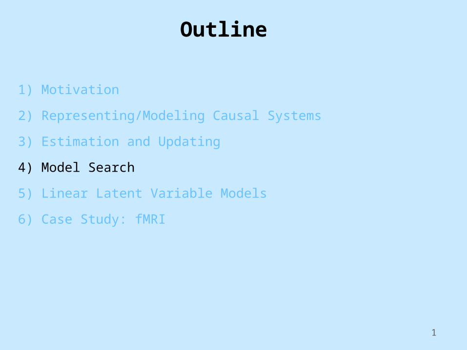
Outline
1) Motivation
2) Representing/Modeling Causal Systems
3) Estimation and Updating
4) Model Search
5) Linear Latent Variable Models
6) Case Study: fMRI
1
Outline
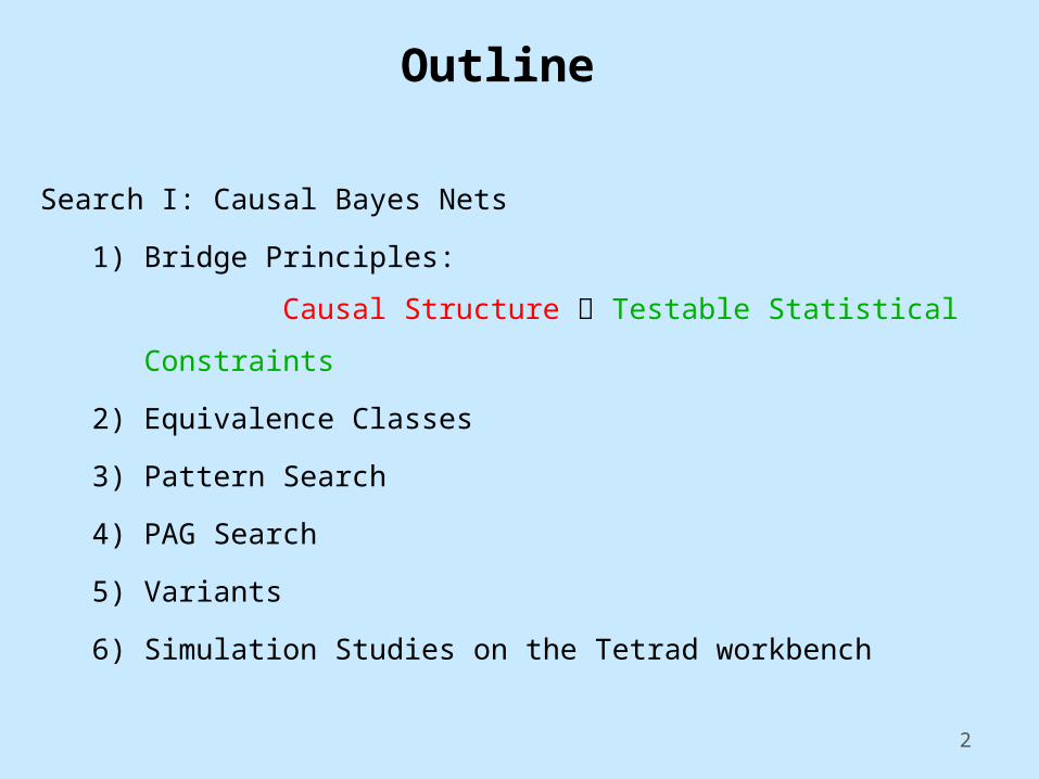
Search I: Causal Bayes Nets
1) Bridge Principles:
Causal Structure Testable Statistical Constraints
2) Equivalence Classes
3) Pattern Search
4) PAG Search
5) Variants
6) Simulation Studies on the Tetrad workbench
2
3
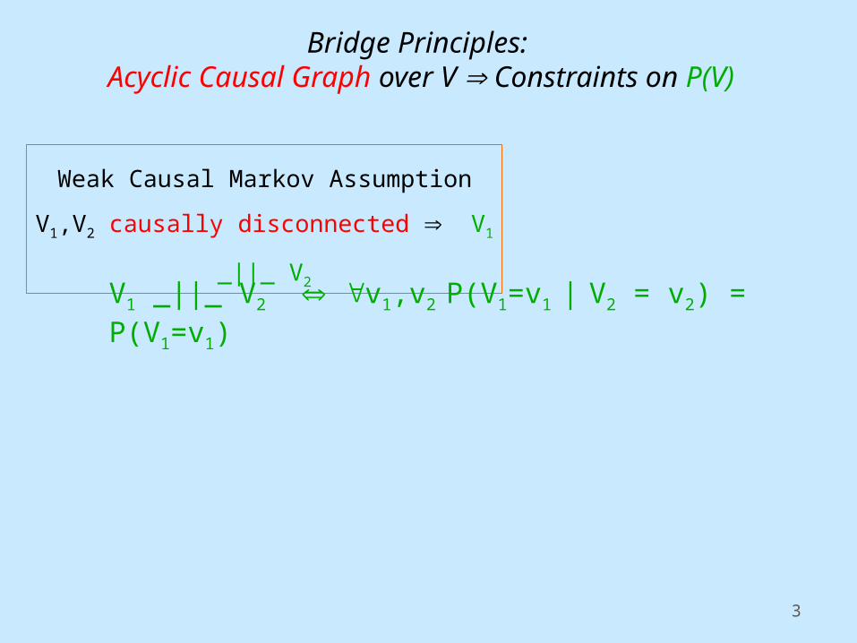
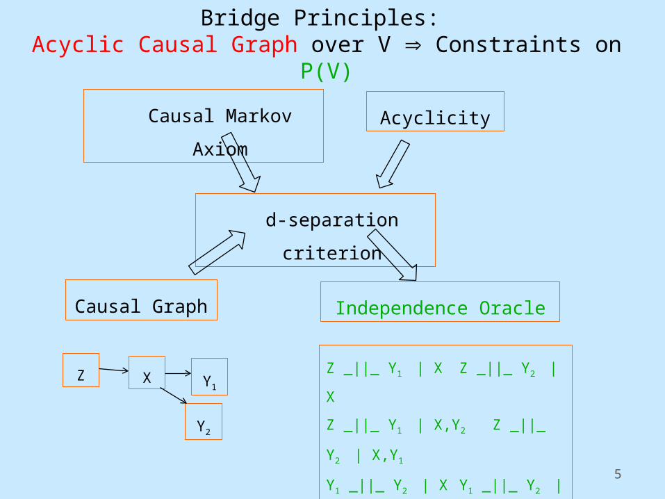
Bridge Principles: Acyclic Causal Graph over V Constraints on P(V)
Weak Causal Markov Assumption
V1,V2 causally disconnected V1 _||_ V2
V1 _||_ V2 v1,v2 P(V1=v1 | V2 = v2) = P(V1=v1)
4
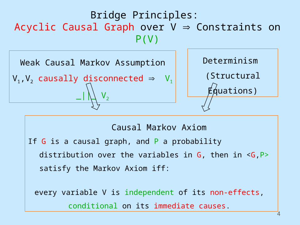
Bridge Principles: Acyclic Causal Graph over V Constraints on P(V)
Weak Causal Markov Assumption
V1,V2 causally disconnected V1 _||_ V2
Causal Markov Axiom
If G is a causal graph, and P a probability distribution over the variables in
G, then in <G,P> satisfy the Markov Axiom iff:
every variable V is independent of its non-effects,
conditional on its immediate causes.
Determinism
(Structural Equations)
5
Causal Markov Axiom Acyclicity
d-separation criterion
Independence OracleCausal Graph
Z X Y1
Z _||_ Y1 | X Z _||_ Y2 | X
Z _||_ Y1 | X,Y2 Z _||_ Y2 | X,Y1
Y1 _||_ Y2 | X Y1 _||_ Y2 | X,ZY2
Bridge Principles: Acyclic Causal Graph over V Constraints on P(V)
6
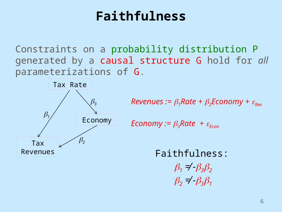
Faithfulness
Constraints on a probability distribution P generated by a causal structure G hold for all parameterizations of G.
Revenues := b1Rate + b2Economy + eRev
Economy := b3Rate + eEcon
Faithfulness:
b1 ≠ -b3b2
b2 ≠ -b3b1
Tax Rate
Economy
Tax Revenues
b1
b3
b2
7
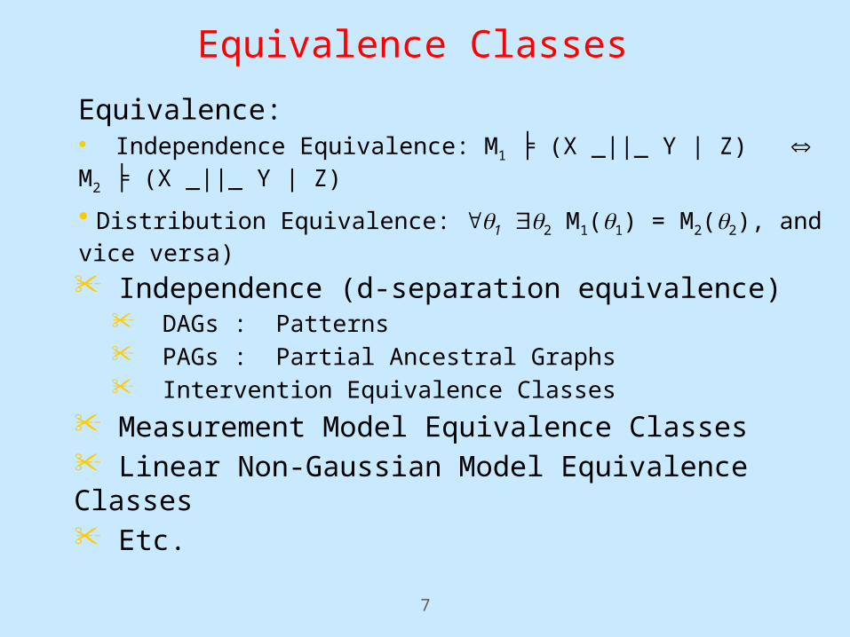
Equivalence Classes
• Independence (d-separation equivalence)• DAGs : Patterns• PAGs : Partial Ancestral Graphs• Intervention Equivalence Classes
• Measurement Model Equivalence Classes• Linear Non-Gaussian Model Equivalence Classes• Etc.
Equivalence:• Independence Equivalence: M1 ╞ (X _||_ Y | Z) M2 ╞ (X _||_ Y | Z)
• Distribution Equivalence: q1 q2 M1(q1) = M2(q2), and vice versa)
8
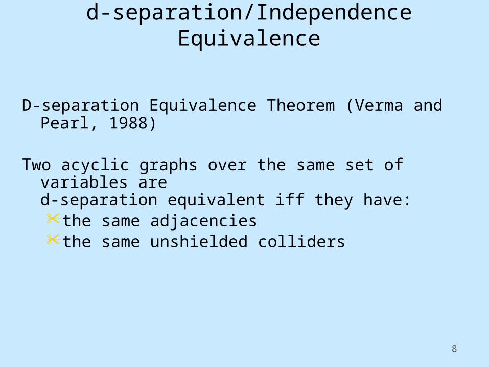
D-separation Equivalence Theorem (Verma and Pearl, 1988) Two acyclic graphs over the same set of variables are
d-separation equivalent iff they have: • the same adjacencies• the same unshielded colliders
d-separation/Independence Equivalence
9
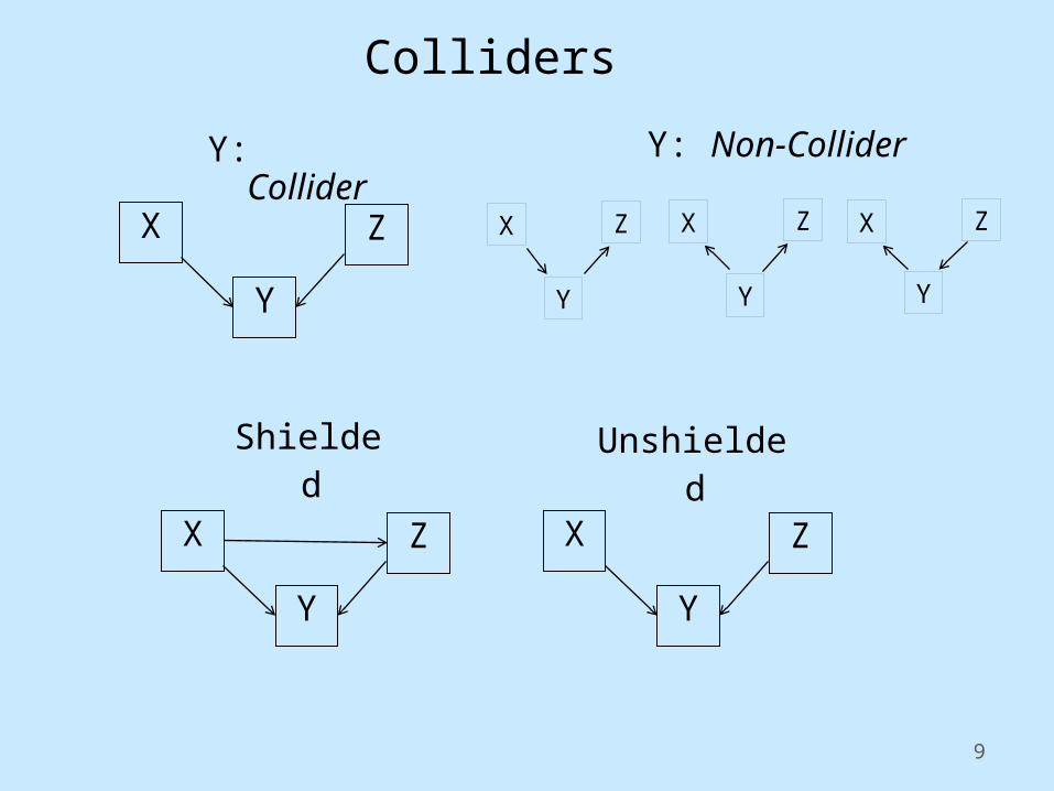
Colliders
Y: Collider
Shielded Unshielded
X
Y
Z
X
Y
Z X
Y
Z
Y: Non-Collider X
Y
Z X
Y
ZX
Y
Z
10
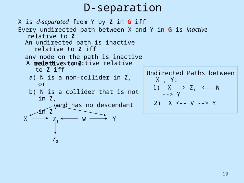
D-separationX is d-separated from Y by Z in G iffEvery undirected path between X and Y in G is inactive relative to Z
An undirected path is inactive relative to Z iffany node on the path is inactive relative to Z
A node N is inactive relative to Z iffa) N is a non-collider in Z, orb) N is a collider that is not in Z,
and has no descendant in Z
X YZ1
Z2
V
W
Undirected Paths between X , Y:
1) X --> Z1 <-- W --> Y
2) X <-- V --> Y
11
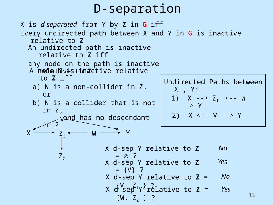
D-separationX is d-separated from Y by Z in G iffEvery undirected path between X and Y in G is inactive relative to Z
An undirected path is inactive relative to Z iffany node on the path is inactive relative to Z
A node N is inactive relative to Z iffa) N is a non-collider in Z, orb) N is a collider that is not in Z,
and has no descendant in Z
X YZ1
Z2
V
W
Undirected Paths between X , Y:
1) X --> Z1 <-- W --> Y
2) X <-- V --> Y
X d-sep Y relative to Z = {V} ?
X d-sep Y relative to Z = {V, Z1 } ?
X d-sep Y relative to Z = {W, Z2 } ?
No
Yes
No
X d-sep Y relative to Z = ?
Yes
12
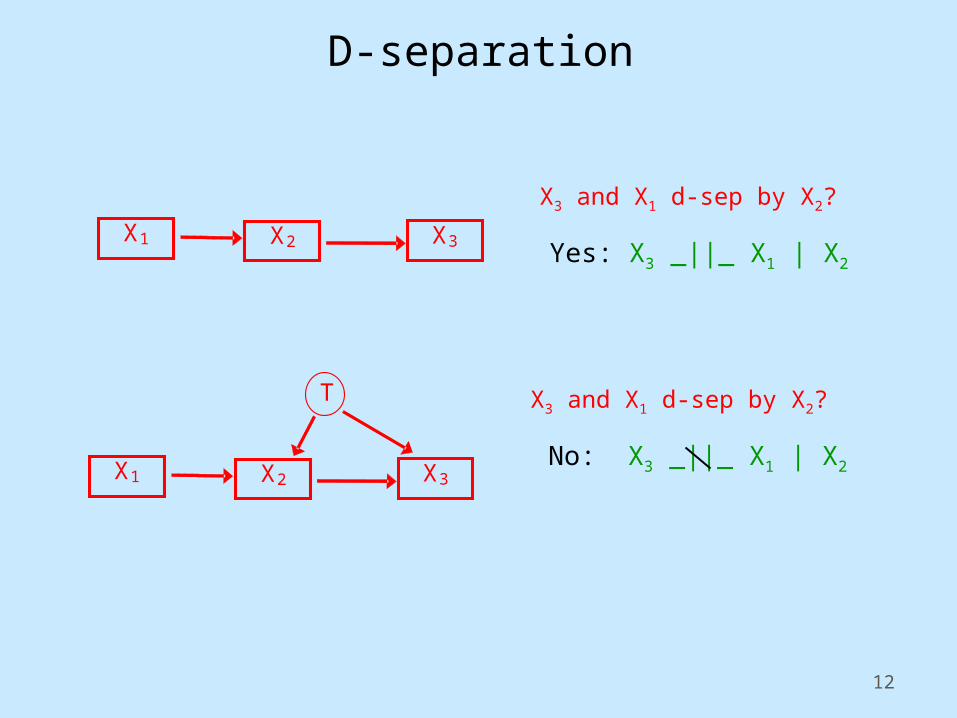
D-separation
X3 X2 X1
X3 and X1 d-sep by X2?
Yes: X3 _||_ X1 | X2
X3
T
X2 X1
X3 and X1 d-sep by X2?
No: X3 _||_ X1 | X2
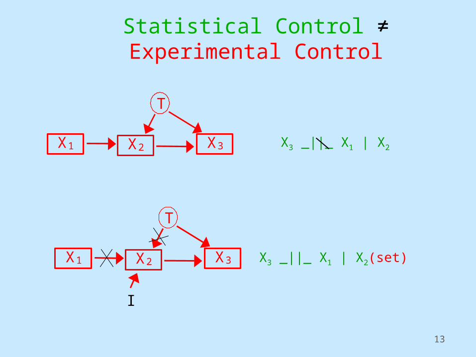
13
Statistical Control ≠ Experimental Control
X3
T
X2 X1
X3
T
X2 X1
I
X3 _||_ X1 | X2
X3 _||_ X1 | X2(set)
14
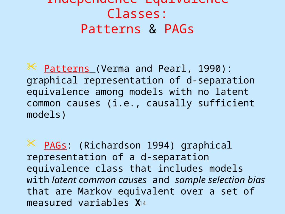
Independence Equivalence Classes:Patterns & PAGs
• Patterns (Verma and Pearl, 1990): graphical representation of d-separation equivalence among models with no latent common causes (i.e., causally sufficient models)
• PAGs: (Richardson 1994) graphical representation of a d-separation equivalence class that includes models with latent common causes and sample selection bias that are Markov equivalent over a set of measured variables X
15
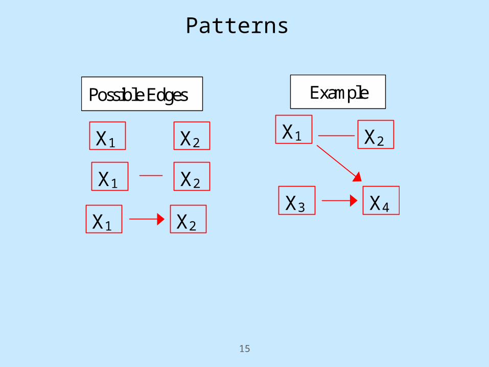
Patterns
X2 X1
X2 X1
X2 X1
X4 X3
X2 X1
Possible Edges Example
16
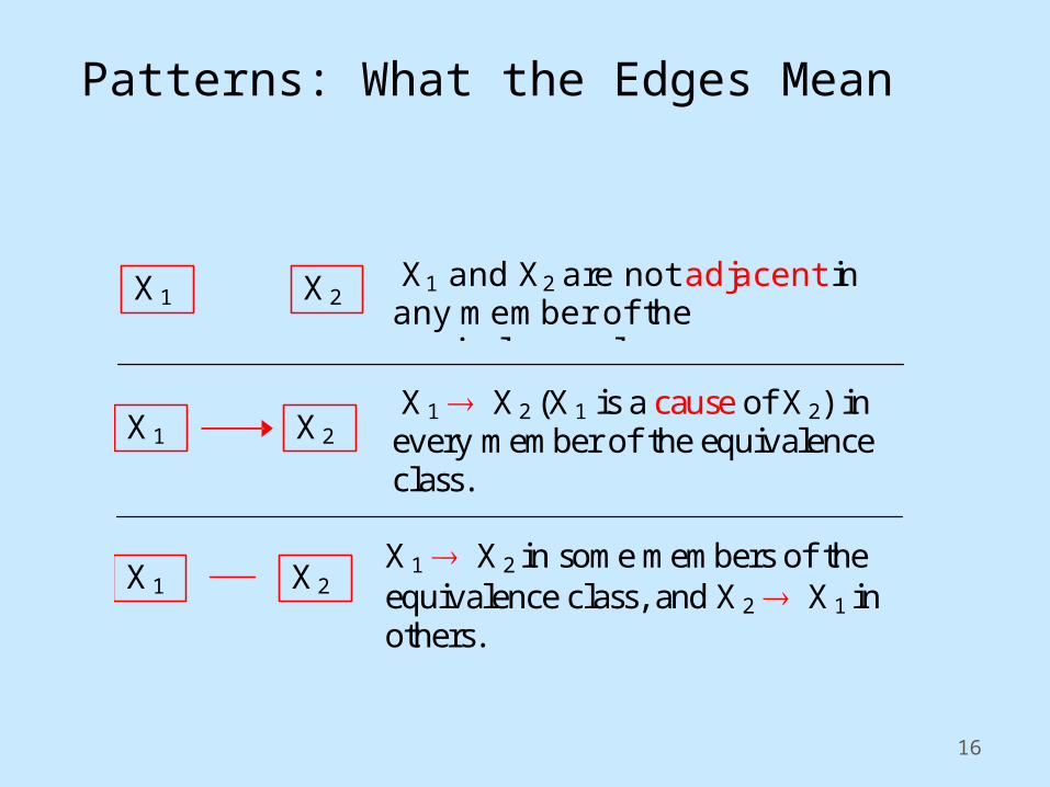
Patterns: What the Edges Mean
X2 X1
X2 X1 X1 X2 in some members of the equivalence class, and X2 X1 in others.
X1 X2 (X1 is a cause of X2) in every member of the equivalence class.
X2 X1 X1 and X2 are not adjacent in any member of the equivalence class
17
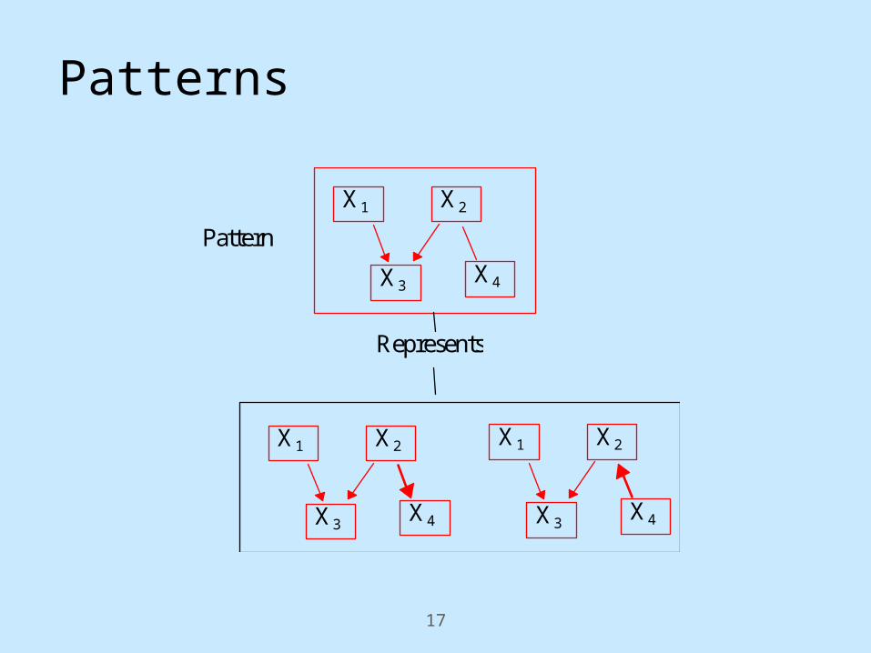
Patterns
X2
X4 X3
X1
X2
X4 X3
Represents
Pattern
X1 X2
X4 X3
X1
18
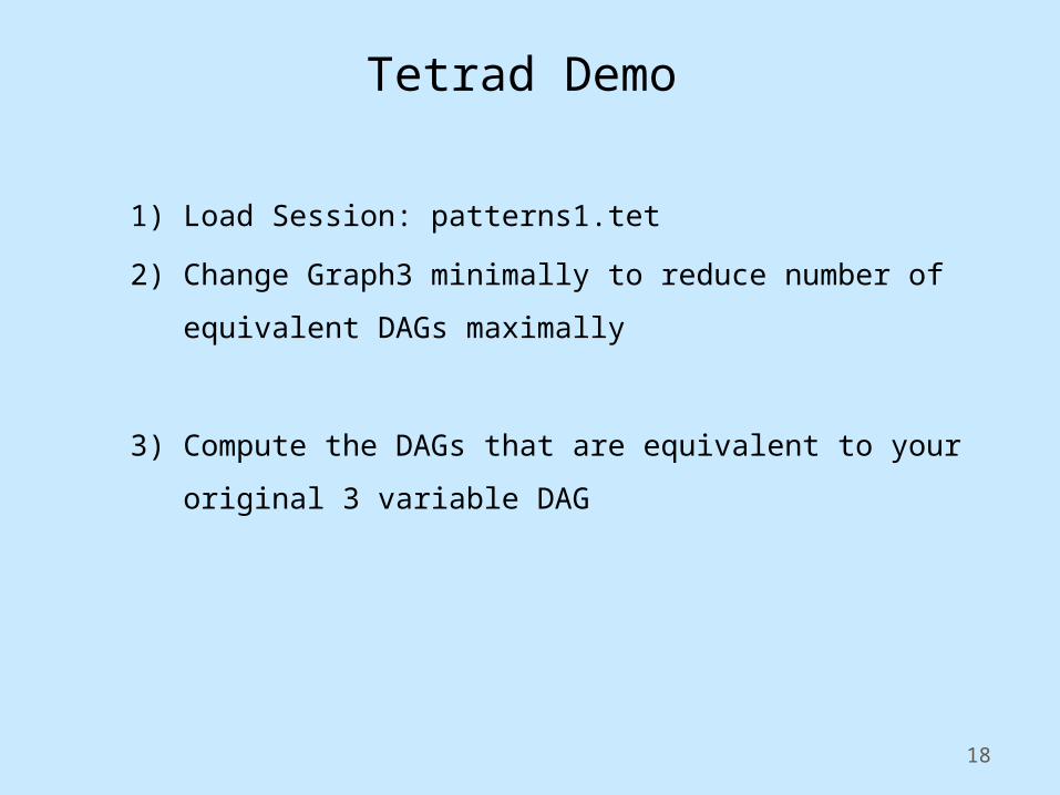
Tetrad Demo
1) Load Session: patterns1.tet
2) Change Graph3 minimally to reduce number of equivalent
DAGs maximally
3) Compute the DAGs that are equivalent to your original 3
variable DAG
19
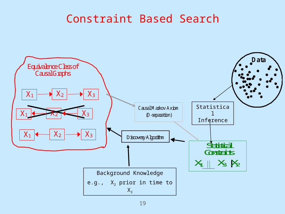
Constraint Based Search
Background Knowledge
e.g., X2 prior in time to X3
X3 | X2 X1
Statistical Constraints
Data
Statistical Inference
X2 X3 X1
Equivalence Class of Causal Graphs
X2 X3 X1
X2 X3 X1
Discovery Algorithm
Causal Markov Axiom (D-separation)
20
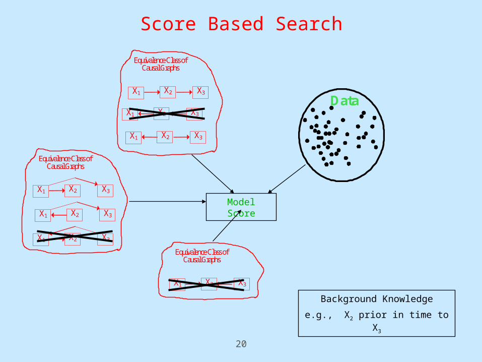
Score Based Search
Background Knowledge
e.g., X2 prior in time to X3
Data
Model Score
X2 X3 X1
Equivalence Class of Causal Graphs
X2 X3 X1
X2 X3 X1
Equivalence Class of Causal Graphs
X2 X3 X1
X2 X3 X1
X2 X3 X1
Equivalence Class of Causal Graphs
X2 X3 X1
21
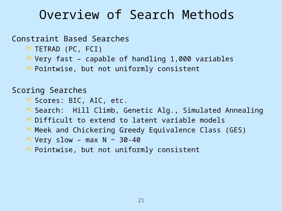
Overview of Search Methods
Constraint Based Searches• TETRAD (PC, FCI)• Very fast – capable of handling 1,000 variables• Pointwise, but not uniformly consistent
Scoring Searches• Scores: BIC, AIC, etc.• Search: Hill Climb, Genetic Alg., Simulated Annealing• Difficult to extend to latent variable models• Meek and Chickering Greedy Equivalence Class (GES)• Very slow – max N ~ 30-40• Pointwise, but not uniformly consistent
22
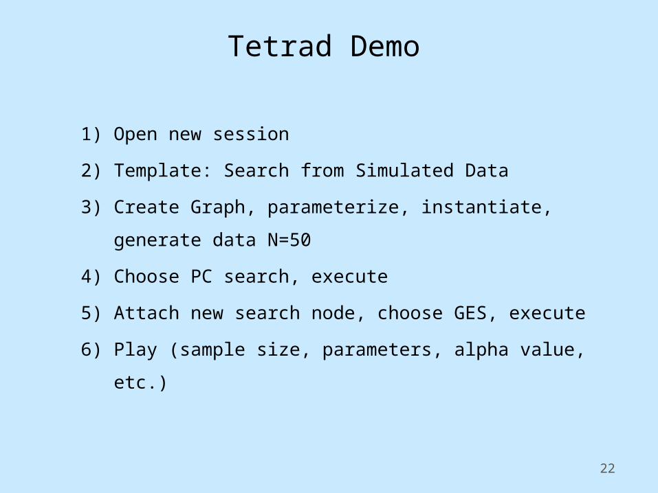
Tetrad Demo
1) Open new session
2) Template: Search from Simulated Data
3) Create Graph, parameterize, instantiate, generate data N=50
4) Choose PC search, execute
5) Attach new search node, choose GES, execute
6) Play (sample size, parameters, alpha value, etc.)
23
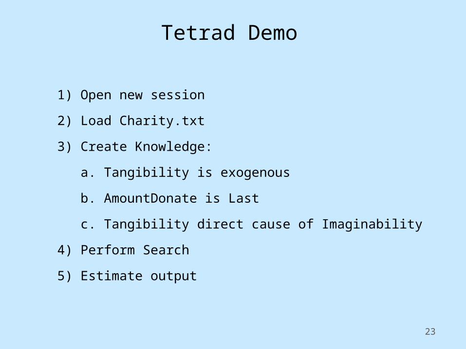
Tetrad Demo
1) Open new session
2) Load Charity.txt
3) Create Knowledge:
a. Tangibility is exogenous
b. AmountDonate is Last
c. Tangibility direct cause of Imaginability
4) Perform Search
5) Estimate output
24
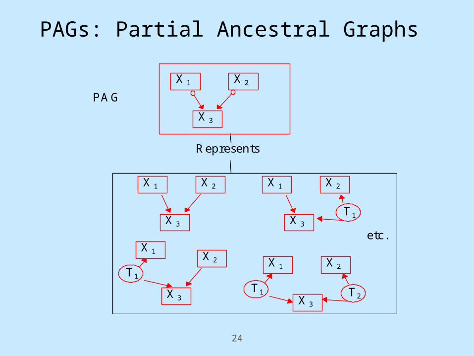
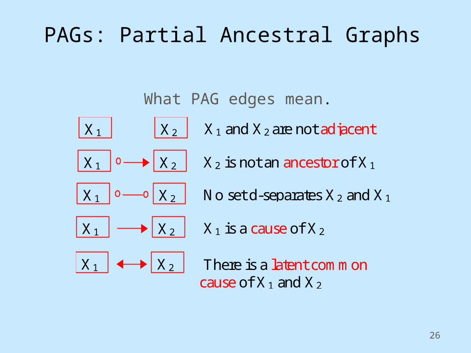
PAGs: Partial Ancestral Graphs
X2
X3
X1
X2
X3
Represents
PAG
X1 X2
X3
X1
X2
X3
T1
X1
X2
X3
X1
etc.
T1
T1 T2
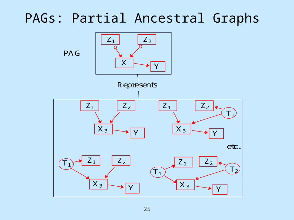
25
PAGs: Partial Ancestral Graphs
Z2
X
Z1
Z2
X3
Represents
PAG
Z1 Z2
X3
Z1
etc.
T1
Y
Y Y
Z2
X3
Z1 Z2
X3
Z1
T2
Y Y
T1
T1
26
PAGs: Partial Ancestral Graphs
X2 X1
X2 X1
X2 X1
X2 There is a latent commoncause of X1 and X2
No set d-separates X2 and X1
X1 is a cause of X2
X2 is not an ancestor of X1
X1
X2 X1 X1 and X2 are not adjacent
What PAG edges mean.
27
1) Adjacency2) Orientation
Constraint-based Search
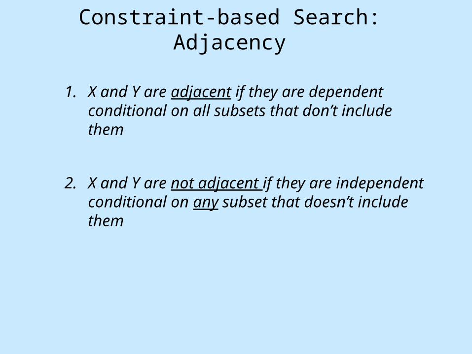
Constraint-based Search: Adjacency
1. X and Y are adjacent if they are dependent conditional on all subsets that don’t include them
2. X and Y are not adjacent if they are independent conditional on any subset that doesn’t include them

Search: Orientation
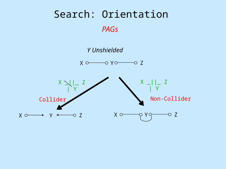
Patterns
Y Unshielded
X Y Z
X _||_ Z | YX _||_ Z | Y
Collider Non-Collider
X Y Z X Y Z
X Y Z
X Y Z
X Y Z
Search: Orientation
PAGs
Y Unshielded
X Y Z
X _||_ Z | YX _||_ Z | Y
Collider Non-Collider
X Y Z X Y Z
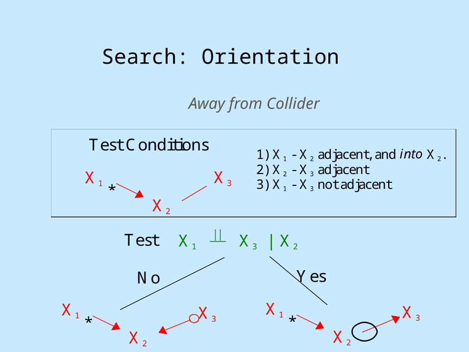
Search: Orientation
X3
X2
* X1
X1 X3 | X2
1) X1 - X2 adjacent, and into X2. 2) X2 - X3 adjacent 3) X1 - X3 not adjacent
No Yes
X3
X2
* X1 X3
X2
* X1
Test
Test Conditions
Away from Collider
X1
X2
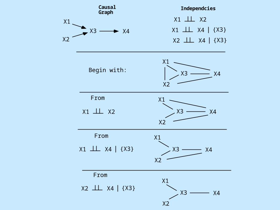
X3 X4
Causal Graph
Independcies
Begin with:
From
X1
X2
X3 X4
X1 X2
X1 X4 {X3}
X2 X4 {X3}
X1
X2
X3 X4
X1
X2
X3 X4
X1
X2
X3 X4
From
From
X1 X2
X1 X4 {X3}
X2 X4 {X3}
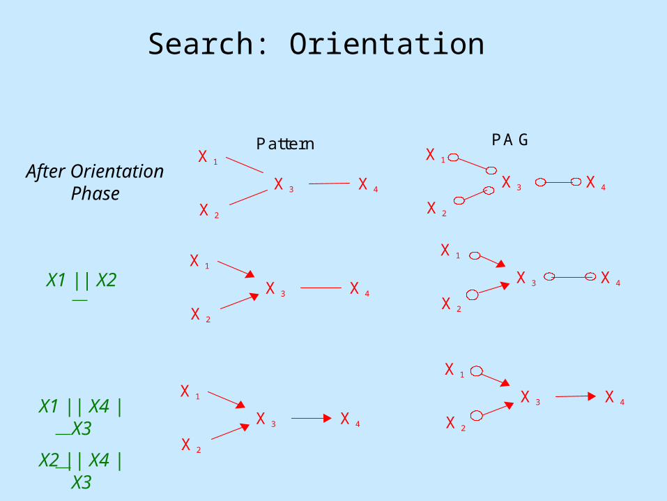
Search: Orientation
X4 X3
X2
X1
X4 X3
X2
X1
X4 X3
X2
X1
X4 X3
X2
X1
X4 X3
X2
X1
PAG Pattern
X4 X3
X2
X1
X1 || X2
X1 || X4 | X3
X2 || X4 | X3
After Orientation Phase
34
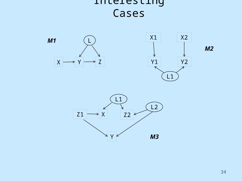
Interesting Cases
X Y Z
L
X
Y
Z2
L1
M1M2
M3
Z1L2
X1
Y2
L1
Y1
X2
35
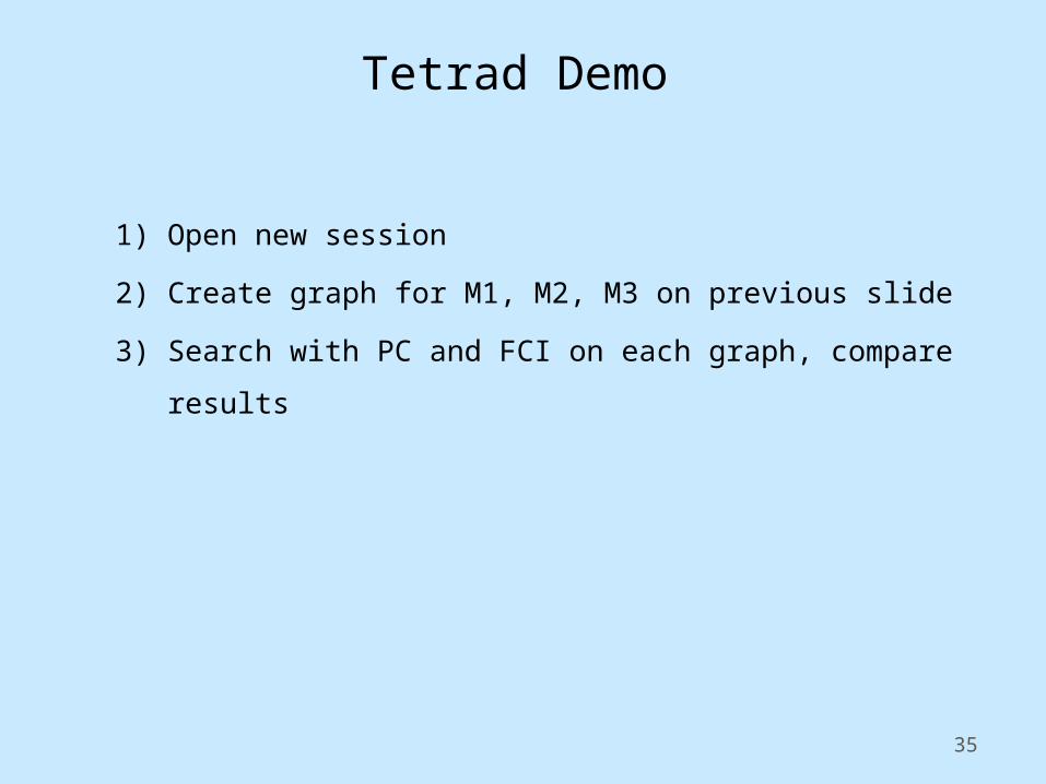
Tetrad Demo
1) Open new session
2) Create graph for M1, M2, M3 on previous slide
3) Search with PC and FCI on each graph, compare results
36
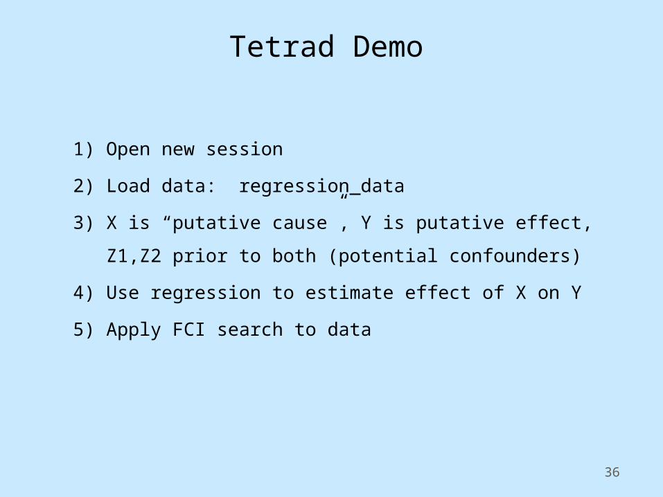
Tetrad Demo
1) Open new session
2) Load data: regression_data
3) X is “putative cause”, Y is putative effect,
Z1,Z2 prior to both (potential confounders)
4) Use regression to estimate effect of X on Y
5) Apply FCI search to data
37
Variants
1) CPC, CFCI
2) Lingam
LiNGAM
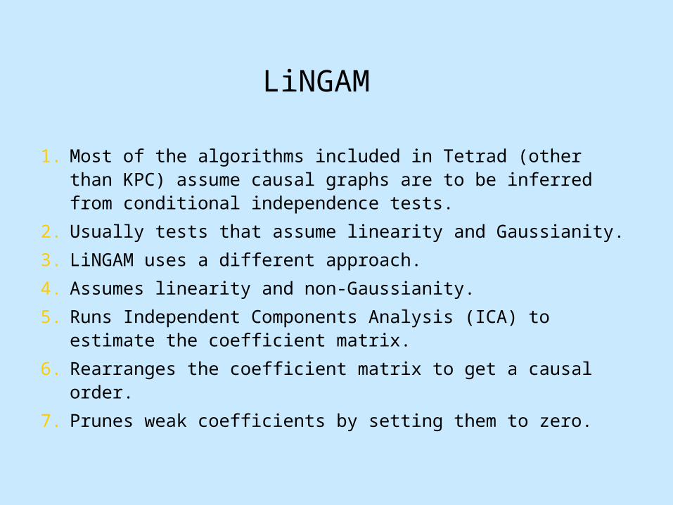
1. Most of the algorithms included in Tetrad (other than KPC) assume causal graphs are to be inferred from conditional independence tests.
2. Usually tests that assume linearity and Gaussianity.
3. LiNGAM uses a different approach.
4. Assumes linearity and non-Gaussianity.
5. Runs Independent Components Analysis (ICA) to estimate the coefficient matrix.
6. Rearranges the coefficient matrix to get a causal order.
7. Prunes weak coefficients by setting them to zero.
ICA
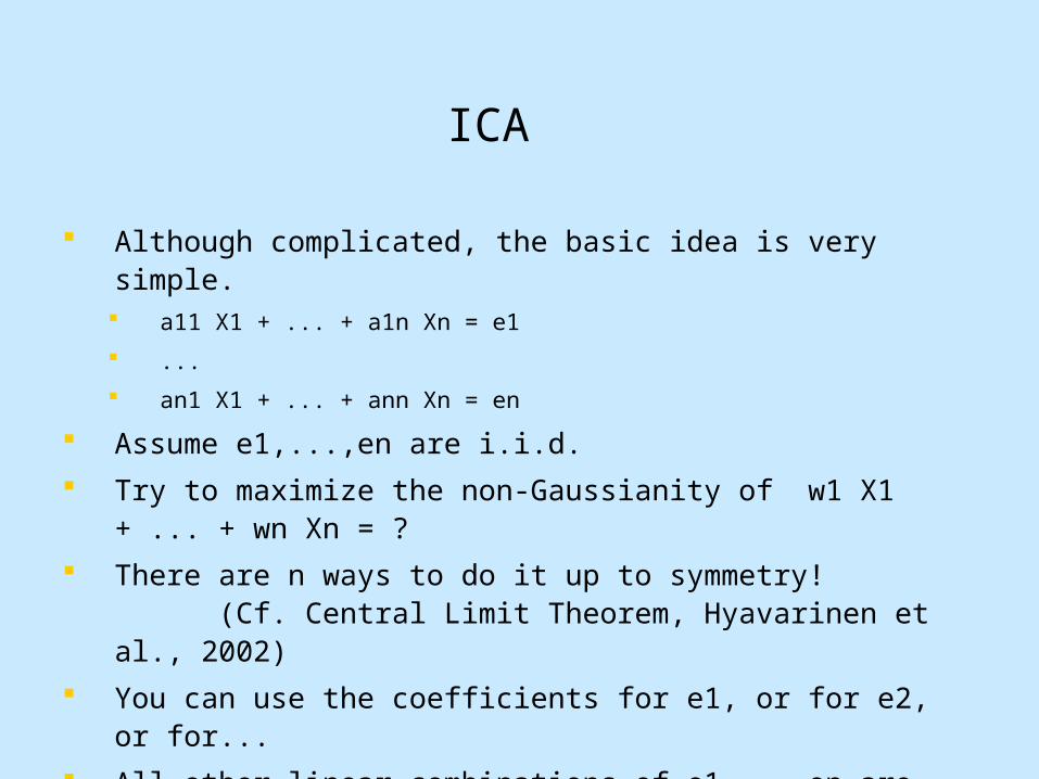
Although complicated, the basic idea is very simple. a11 X1 + ... + a1n Xn = e1
...
an1 X1 + ... + ann Xn = en
Assume e1,...,en are i.i.d.
Try to maximize the non-Gaussianity of w1 X1 + ... + wn Xn = ?
There are n ways to do it up to symmetry! (Cf. Central Limit Theorem, Hyavarinen et al., 2002)
You can use the coefficients for e1, or for e2, or for...
All other linear combinations of e1,...,en are more Gaussian.
ICA
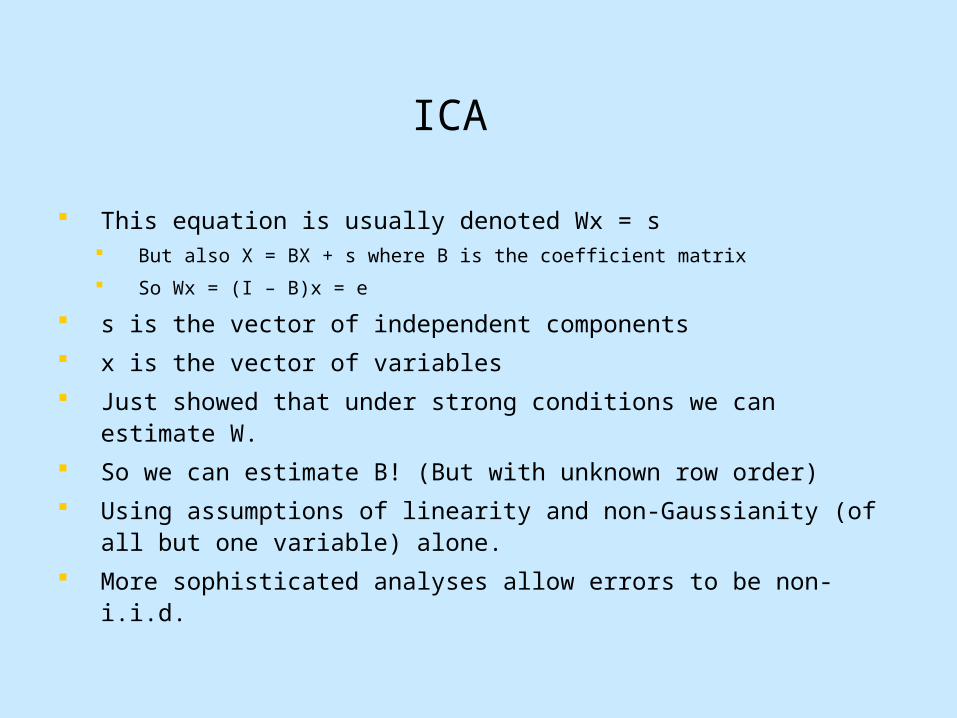
This equation is usually denoted Wx = s But also X = BX + s where B is the coefficient matrix
So Wx = (I – B)x = e
s is the vector of independent components
x is the vector of variables
Just showed that under strong conditions we can estimate W.
So we can estimate B! (But with unknown row order)
Using assumptions of linearity and non-Gaussianity (of all but one variable) alone.
More sophisticated analyses allow errors to be non-i.i.d.
LiNGAM
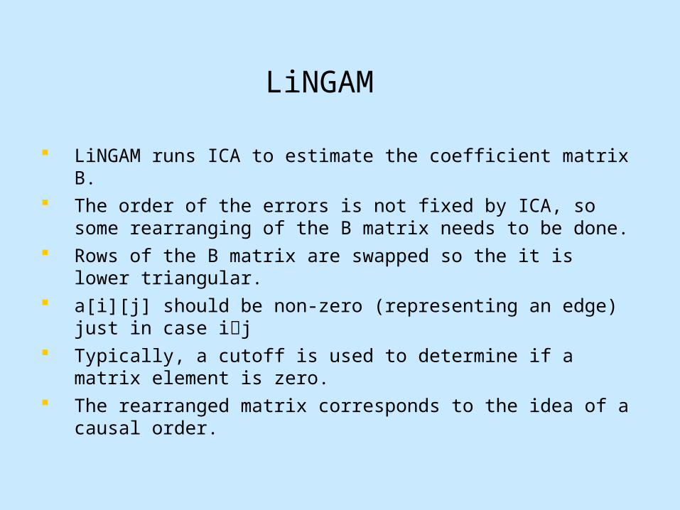
LiNGAM runs ICA to estimate the coefficient matrix B. The order of the errors is not fixed by ICA, so some rearranging of
the B matrix needs to be done. Rows of the B matrix are swapped so the it is lower triangular. a[i][j] should be non-zero (representing an edge) just in case ij Typically, a cutoff is used to determine if a matrix element is zero. The rearranged matrix corresponds to the idea of a causal order.
LiNGAM
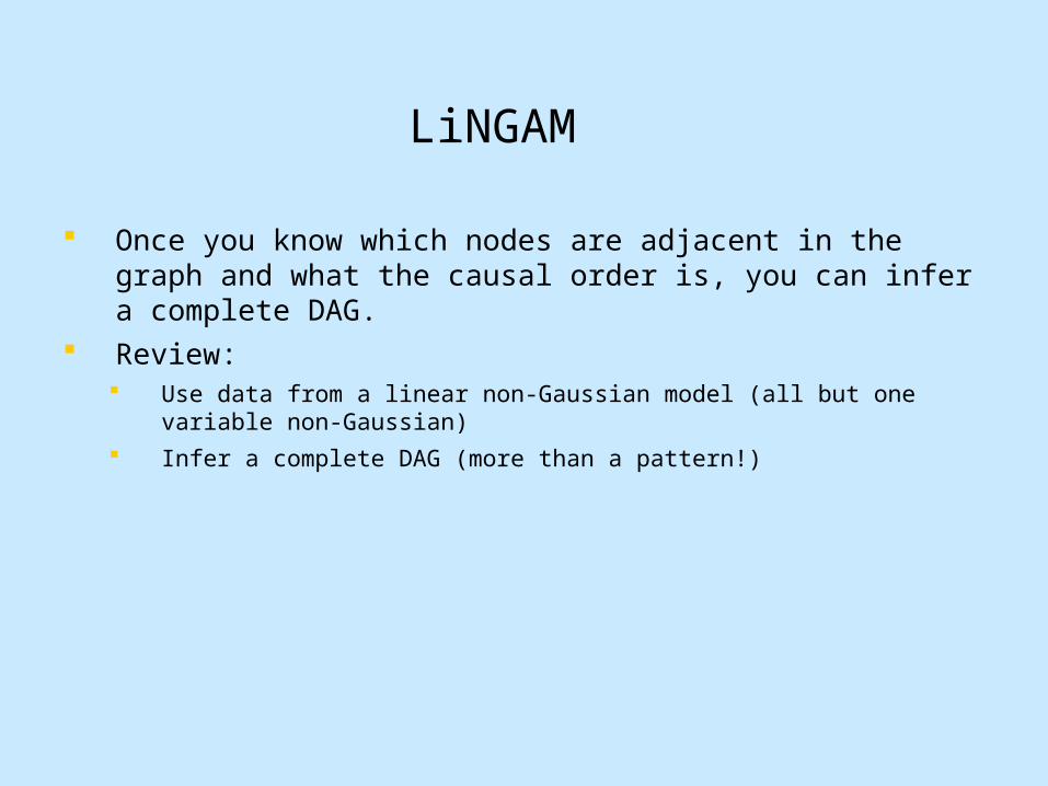
Once you know which nodes are adjacent in the graph and what the causal order is, you can infer a complete DAG.
Review: Use data from a linear non-Gaussian model (all but one variable non-
Gaussian)
Infer a complete DAG (more than a pattern!)
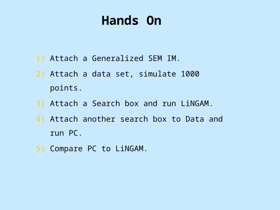
Hands On
1) Attach a Generalized SEM IM.
2) Attach a data set, simulate 1000 points.
3) Attach a Search box and run LiNGAM.
4) Attach another search box to Data and run PC.
5) Compare PC to LiNGAM.
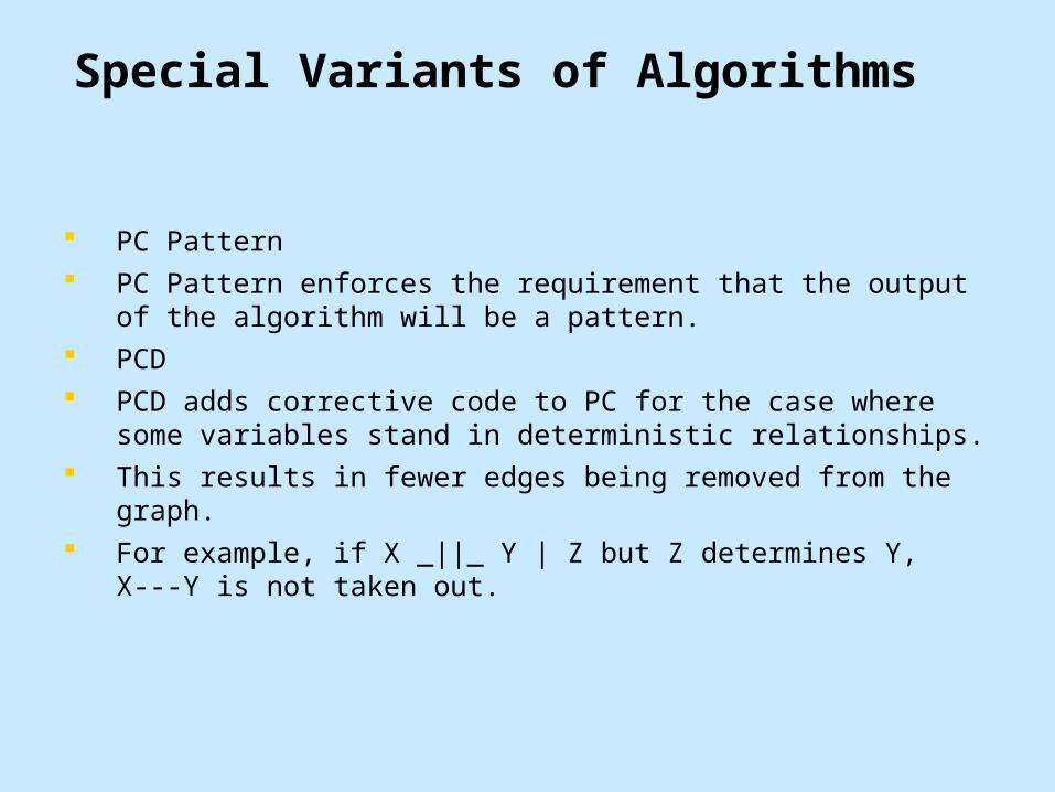
Special Variants of Algorithms
PC Pattern PC Pattern enforces the requirement that the output of the algorithm
will be a pattern. PCD PCD adds corrective code to PC for the case where some variables
stand in deterministic relationships. This results in fewer edges being removed from the graph. For example, if X _||_ Y | Z but Z determines Y, X---Y is not taken out.
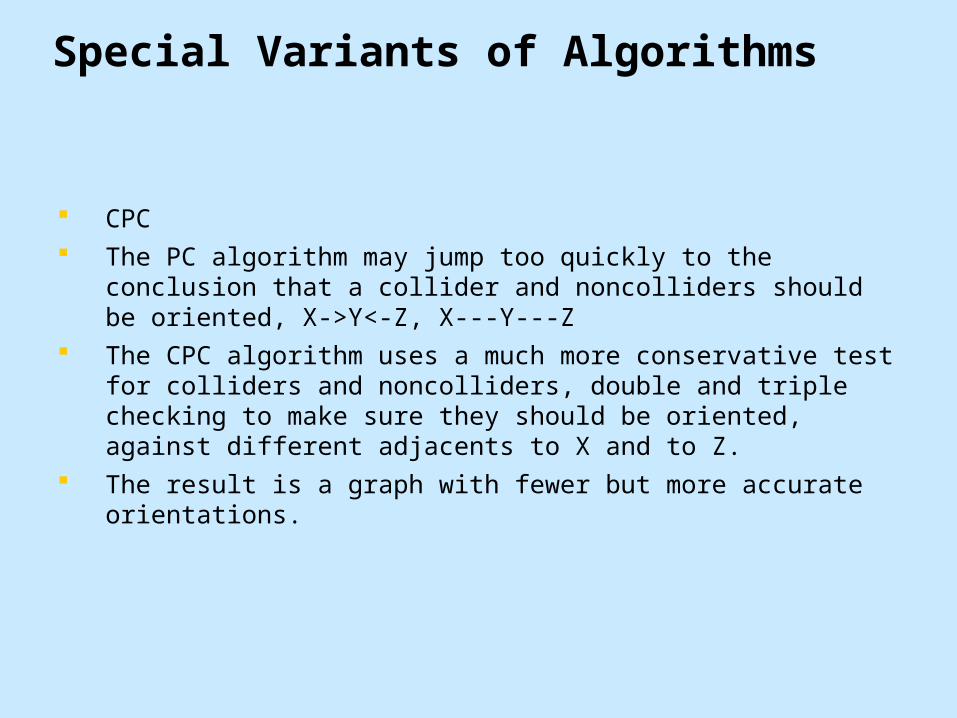
Special Variants of Algorithms
CPC The PC algorithm may jump too quickly to the conclusion that a
collider and noncolliders should be oriented, X->Y<-Z, X---Y---Z The CPC algorithm uses a much more conservative test for colliders
and noncolliders, double and triple checking to make sure they should be oriented, against different adjacents to X and to Z.
The result is a graph with fewer but more accurate orientations.
Hands On
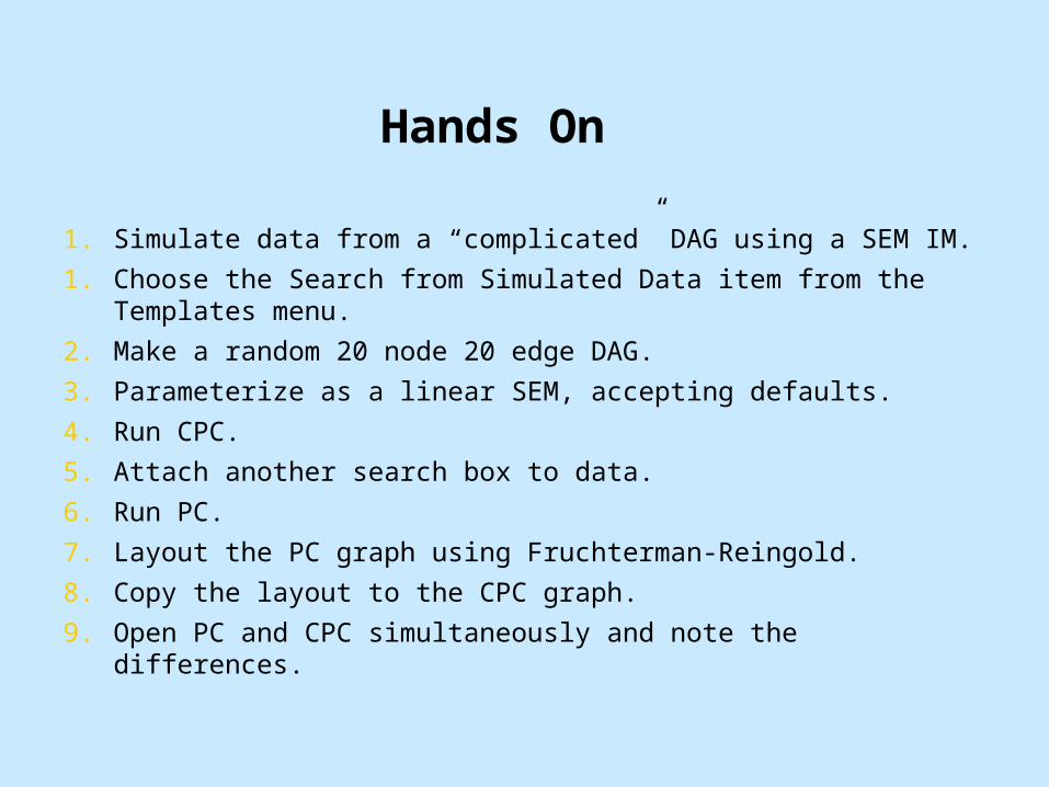
1. Simulate data from a “complicated” DAG using a SEM IM.
1. Choose the Search from Simulated Data item from the Templates menu.
2. Make a random 20 node 20 edge DAG.
3. Parameterize as a linear SEM, accepting defaults.
4. Run CPC.
5. Attach another search box to data.
6. Run PC.
7. Layout the PC graph using Fruchterman-Reingold.
8. Copy the layout to the CPC graph.
9. Open PC and CPC simultaneously and note the differences.
Special Variants of Algorithms
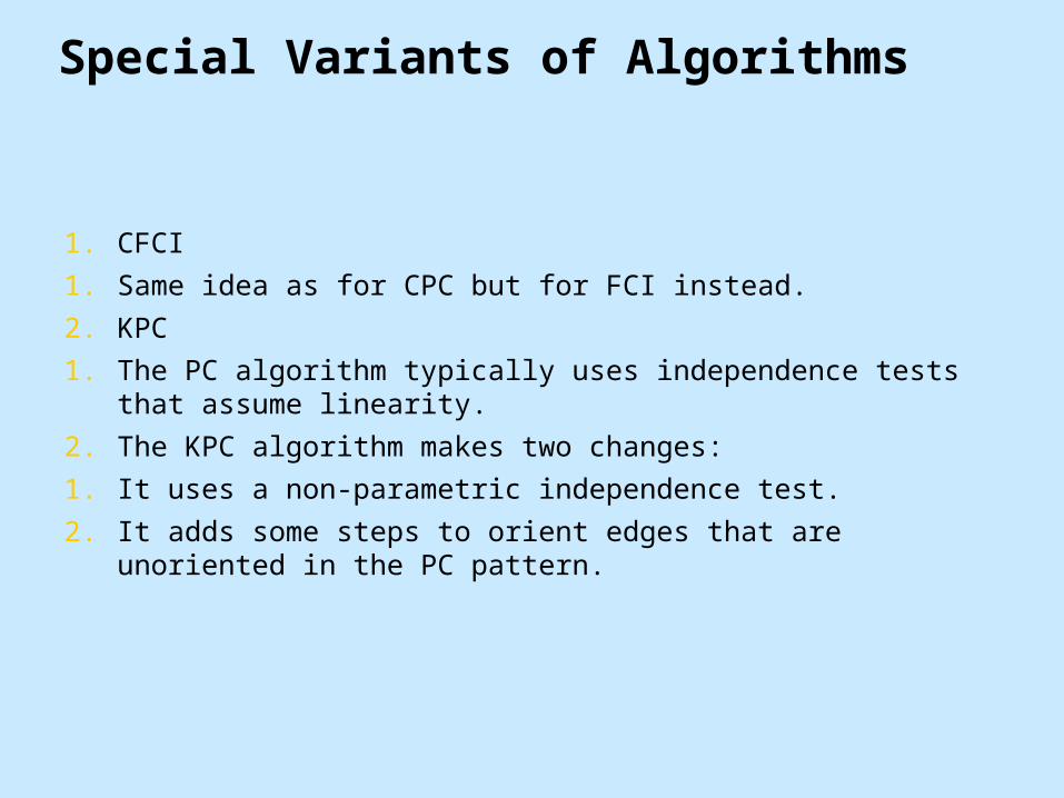
1. CFCI
1. Same idea as for CPC but for FCI instead.
2. KPC
1. The PC algorithm typically uses independence tests that assume linearity.
2. The KPC algorithm makes two changes:
1. It uses a non-parametric independence test.
2. It adds some steps to orient edges that are unoriented in the PC pattern.
Special Variants of Algorithms
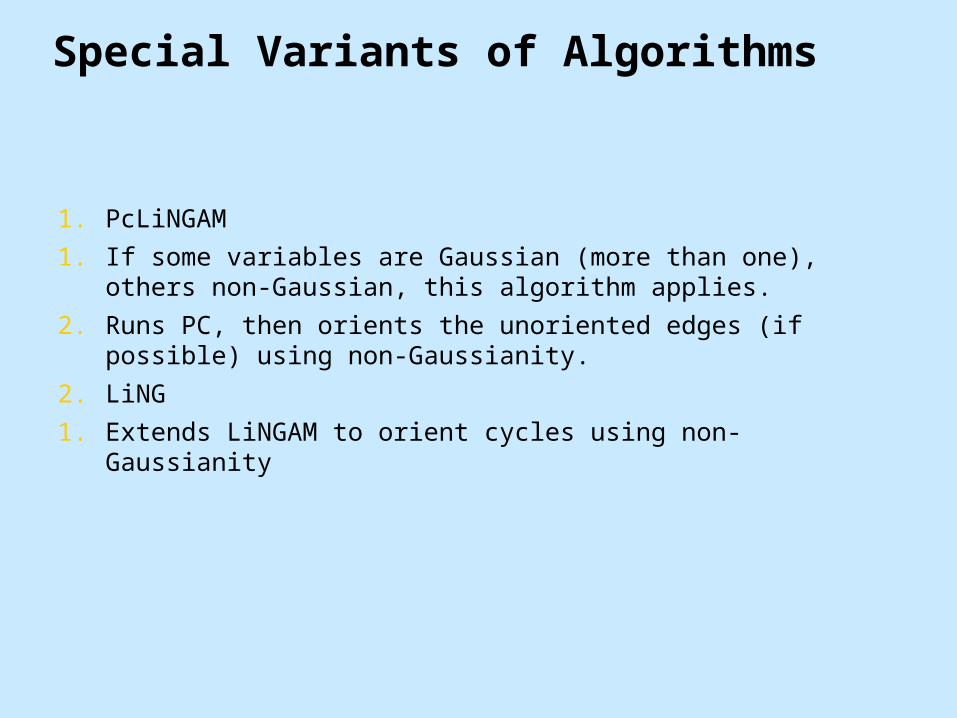
1. PcLiNGAM
1. If some variables are Gaussian (more than one), others non-Gaussian, this algorithm applies.
2. Runs PC, then orients the unoriented edges (if possible) using non-Gaussianity.
2. LiNG
1. Extends LiNGAM to orient cycles using non-Gaussianity
Special Variants of Algorithms
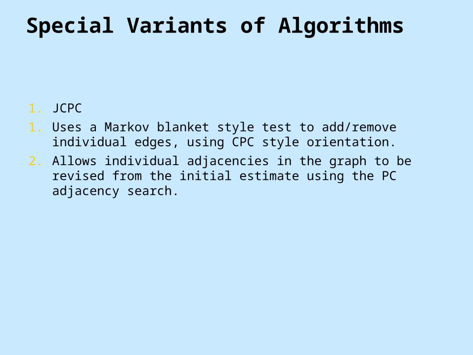
1. JCPC
1. Uses a Markov blanket style test to add/remove individual edges, using CPC style orientation.
2. Allows individual adjacencies in the graph to be revised from the initial estimate using the PC adjacency search.
50
Simulation Studies with Tetrad