Unit - 4PART -A

10 Mention the importance of geometric tolerancing. (N/D -15)

..s: f;z..L. €If ...i::n oU V.L oLu.~ J~~ t:WI tJ aJ,U:J t;K),.,_h1,# Vo·"'; a...h 0'-'

/o.e.hve.eA .f~~.

2. Define the following terms: (a) Interference fit (b) Running and sliding fit. (N/D - 15)

tal..L ~ ion Of tJ n.I- pov.-t J.b!J U~ e 'Z C.Cltul..LJ f1..t.- J:n foe "if'rvJ

f?(t MLNS , an Of h-4 P ov:J" ..z, ()J to N c,J.. .li; ~ to.JAk.

~ at'l U :!A.J:;r fa'l' t..a f...u, ~ 1Y>A!j biz c(..td A..c..A1tJ U. (wr ("N,

...1 NA- If /:p .(..{) ~ O}"..I'.k. ch. 1- f'.Li.La w.iJf1)..8? ~. t....?k .

___ •• _ o. _. __ ••

3. What is meant by assembly modelling? (M/J - 16)

Aff)V'(}h.~ ""o~~3 ,.e., .::l. ./·~/U...olo!J~ ~ IYlLfhoJ

~ ~ ba e» 0 S fl fe ~ fy A.." cI.J..L to u,·("Ji p..u .f~ .o J..-i c.A

4. 'Whatare the uses of tolerance stack-ups? (MJJ - 16)

~ ku. €.\I e.A- rn 0 A.6.- ,..,.,a,.n 0 N... f'{) J...ur.~ j,.A. ._j}, ~ .5tv ~

olCU. c.i' O? o..-tt~~ #L..Lo ~Q;J of c::- J.l tltfl J'v. .....1tA v. ".f t\. p,.d-,.

fo.u.'rtvl c..e.o eu..L eu,.n:. ..J-,."·f1/1t .

VJ~

5. List out four parameters which are calculated by mass property calculations. (N/D - 16)

b· Duw.~

c,.. V'o...u..vnc

ot· R r.lf fY)() ~ of ....vu.,-,.; Gl

Q, Se: WI') c1 morf\L;...f O.f -irJ o--J,'C)(

f . ~.l d 0 r- c..t.,,.._.f.J..L ()., 8A CVJ..i..Jy

6. Define assembly modeling (N/D-16)

Am~b.~ oJ....u.J.1t1~ (.£)~...t.., b of -two OT 1Y).()..u...

to~ 0 ~ (Vr') e-«1 b.J...ul fY.J e: rr-e« a.t- ~A. ~ fX2-.~.J; viZ

wo·rt(_ pOJ r rvo-s fA/J.&:/ p~M c .JvLlo'£iOM.

D e....t c..A-Lb e 1"N. b0 fI-O n? v...p a..., cd h:7p at t)'a..() /') ~ em b~

~.-(8n w~ e')LCVl')p..A...tA- f_Nlo- fb]

'7"4 a-n ~-'Y> b~ rr» e ~6 p-A..Qe.tA? ~ t!..4 be...s~ w ~

e~ 0 a.. b~ it ~ ~ b~ ""'<J~ tA.d.in (} ~ dfl-n _" bkJ InCPJL

4 we.. C2. ko.rt~ <fN_ Orl- 9~ J. P ~ , we. CAe> e.."'__'""" aJ..t. ..L.h

c..OO .,g +-0011 ~ ~ eu> ~ (l.rf') ~ ~ h:j J.un p.l.tJ o.p t1l~" ffl_ tJtm ern b~ •

1'1...L ... e. ...ta, ~ buw e.PP (U') ;OW:>eff> bLtJ ,."d.ih ~ ~ v.t otc-t,v p ~ J4 ~

MIJJ ~ . .../)r') p 0 ,-t-~ ~ c1.a..t'N-,J-,J C() fI t£p +- be...A.t:nd ~ 4!I'n b .':!I N) c ~ fJ .

1Y>Q4.(~ ~ ~.AL-r ~ t:I ./....em p.At y & m~rf-a.fc -rr«: J.J.a.,I1 Of) -d A4> oS a.r..J

~fU\L~'on be Iv4v} or 01- p~ tfJ,ev) ...e, "._ +t>-p-.:Jo~t') ea..ppypoeJ...

T{}fJ - ol 0 W I") a.-n em h ~ ap p'rlJ ~ c.J,

IN.. <tv p oJ 0 tAlI") a,.pp-ro a.uh ( co ~ 9 t"lJd f<rc ~ -d j ~

a--n (HO h-1J ;..M ....t ~ tI-os ~. a..n €;'f) b A-CtA eo r-.6 •.c:.o ~ Of' +e......

01 <tNJ ~ ~ b OJ eompo f'\LN".> •

'4>p yt) ttl c:.A ~ f'ncVl"" ,,~~ fN- ~../. 9 r» c!J,f ..1.~ aA'> ~ h~ ~

'11- o..il.ot-\d 0.. ('TO Je.cI ~.. ~ ~ ur pro atu.. V ~pe-c..i fr CpJ,'O,J ~.

'"N...t. <+-0 p of 0 IV!' ~ em "41 Of (J...-oct. VI 1-0 £ ~JO a. J '" H. """'d

~ ~ ~~tJ o-p P l"'Oa (;), I:P r=clu. c."f oJ.,tA..I ~ "...in co tv cJo .ff.t,

a..o~b~ ~~ &t:J/'I')rn~ ~ ~..c~ eA,U-eW"\", I:;tJ

,§c.L-b S 'P Ie re» ott.. v~ cp e yO I .,u, c..J..u.. ota-> a .fu..p p_.Ul p. ~ ff4 A...t

CAO NY" ) cJ.,{o v.J-.d d..a I'rl b tAX~ ~ I~ r» ..fea.1'..d ~ 11'./0 riA tol"l CAA 'rr'~ ~

W~,;:,. a CAMIfl~ Py{1 clu eI J~~orta. ~01- ~o ~w...J

ol.<.A-~ J ~.i 0'-' tv /'B£J~ eo f....i).J_ ru. A-'n em b --4J ...t...~ ~ Jc.6

h~8 .J;.i;ntUJ.~.

~ h>p ~ ~ Cl.oY) =» o..ppTOD.. u, /olZ.fJ..l.n.I w~ ~

~fVI'f'J.h~ ~ II1.d ~(U.l-eJ, Lta.-MO IJ_~W<"l ~ .Jlu.J.L·t'()1? mooU)..). I'1""N. J..tu,jlfl,vf

~(!_T'V'e.6 ~ j-N. be.~o( ~ ~ ,g (!JU\..Ul ha..t:..U.-bo...L Of- ML a/Y:> &"I? h-LtJ. ~

~ fItAk ~ aD Ct::Iror-p 0 ~ ~.,.._. ~ Of. (J&#) ~ tvn bltl .

~ e, ~ n-p O~ A.U. 14 e-.p ~ II a.o ~ do,.of- !....Ave ~ W)Ve.,..",J

.J,..g_+e.u-n ~ ~ a._c..huJ.._ p~ CJ,.;\.Cl J u..J:. G'1"'T.) e.n') h.....uu J....:J..u. ..

~. a,..p~ h~ ~ tro.;I- ~ ~ o/..L+c:neo .£4h,rI-.J I _fJp cot ~ C!~ ~

~ ~'r P 1u.p"CA) P 1"0 P ~ rhl~· rt';)~ he tM~ I:l.. ~ 'tk-

8e.c I'Y'(.../'tj 9f 6-Nl. rfI-.L ~ O~kJ ~ t.oIL/'vV ~ (.K)~ or-f.JJ? .

Iv h.A.t tJLo ~ LIU.. MLc.vvC- btl rfcJh. ....a.o UL an ~ io "<

L..o, +- I-f....a. f'Y\.e.t-f..,o ckJ a../) ttA- e 'X.p1cc.k ~ (.7 ~ k d..t:! eiJ .

TN... prO um 01 cN..clu::" () 'tf..t. +o..Lt. T'(;tJJ lL4 /y Vt:I)') f(j

\:t'J IO-lb)

7J.J._ a....<Uu.~ or € ~~

...e, ~ Q._u.<J ~ .

., \ F= m- c.n-mJ 1I ,

b~ a..t::1.~[J ~ rfin'j-. rY) ek..~ ~of .rub ",D~ j

.tk.. ~ t: ( n - m ) e.l.L fY\4!.,._h .

f()

,... ~ L ell'r1'l'1el 'X 'Z.. rt') 0. 'X.

.t = I

-_ .. - _ ....--_ ...

ot.uI 'r ')j bIA.h Or:;

'f rv0 1"1'04 I fN_ (J"'Q b~.w .s rie: &..Lr v e .M dV'(')~ C:! f-..e. A-

1\

.>f ~ 4/) ~ iA f"N._fY..<) tJ P.MJ v...c. o(L!J ,tM ...e:,(;,.~ erJ cI..uJ..f S" ,j..uw &:...tal:::!

b:J ~ "" ~ -IN- CJ4:,..J a r-er ~ d..u, 8n & eu"I':J ~ tJ ..u"e),

l\l ill ~---.-- -._"-: -LP,.J : ",I, 0 ~,.oVI.:fO V\ ...

K:::.'

-------- -- _-'"

-

s {~14/1? I e-h..

e:,'"T"5 e..,p.~ e'X-p...l.Jn rtN- .ft:,,U.o LO,.v..,9 ~".. oU. hon...1. Io.-&..'t'-eu? (..L ~.....Pp ~

f'Qe...ff.._o ~ w.ltf, ex.etAY)p u.., ,

lb ""Or:} f ~ 6v.le ~~J VJ

(t..) eo 0 + .f u.m S«tU-~[N(D _'15J

~ Qoo+ fr..vn ...r~~

[ hlor-rf - ~ .J'+a..IVJrsuJ, ~cI]

t:» to -IS]

,.. - -r ~r

r

IF

//

I-,,

6'.

f).I.l. H-.L CA'to rio OM pA40 ~ --4J Ivwe.. ~ p o~....L !:P

olu...t cA- ~ t:N'I 4 'No f-N_ P OJ Lb.iV l::J t>+ 4 .Ppe t.." {lue:J. ~ EUn b ~ P lICK? -10.,.

~ 'r ~ rv-.p~ a..uJO "., ~ en 01- h.JJ. P A..O ~ ~ Of c~8

pro .f~JoneJ ~~ b~ p~ fI..e.. *'..tLow~8 ~~ I;y ~e pe~+o'S'~.

&J tv-p 0~ Jb .~ .a-r.> e.ff) b ~ ,

~) 'Th..ut .k M I!')..t,oj .1~ loY- uJ-..l ..1.£ ~ ~ ~ B4V) b4J ~ €a foc~.

.~ .P JJJ cJ_"

v

mjjJ ,.dm

roJ> J j S d-'X. d'd' d.'1-

'X ~ ~

""1 ~ x :- jJ S l-jdfY) - J> Jj j ~. ctv,..

J'()v

t--f ~ ~ ~ JJJ z.. of ro ,..p 1J J ".1-. rJ"IY>

\I

0.. .9 tve/' at. ?t;..to ..L:/J e.....~A1 }:# ~ pro du Cf 0+ I-N. mp...D t:A-ttJ. tft-t_ J. ~t'V..L

€)f- ~ pe-rpenc;UcuJM d&J ~tL be..J-wegn ~,.,.,~ ~t:l tfN_ ~~

Part Modeling Assembly modeling Part modeling is complete, valid and unambiguous representations of objects

The part modeling is conversion of 2-d to 3-

d objects by revolve, extrusion, sweep etc.

Assembly modeling is the collection of individual parts.

The assembly is mating of the individual parts

by axis, surface mates etc.

ME6501 – Computer Aided Design

Unit – IV

Part – A

1. Differentiate Part and Assembly modeling

2. Differentiate Bottom-Up assembly and Top-Down assembly approach.

Bottom-Up assembly Top-Down assembly In this approach the individual parts are

created independently and inserted into the

assembly

This is a traditional method which can be

used for hundred or thousand parts

In this approach initially an assembly layout is

created which acts as a backbone which helps to

design the individual parts

In this method the sub-assemblies are managed

which helps to assemble more than thousand

parts

3. Why is that testing the mating conditions necessary? Testing the mating conditions is very necessary as the under constrained object would float or the over

constrained object would lose the required degree of freedom in simulation. Testing of mating conditions

provides the opportunity to ensure that an assembly functions as it is supposed to according to the design.

4. Explain the Inference of position and orientation.

The inference of the position and orientation of a part in an assembly from mating conditions require

computing 4x4 homogenous transformation matrixes from these conditions. This matrix relates the part’s

local coordinate system (part MCS) to the assembly’s global coordinate system (assembly MCS). This

inference of assembly parts result in effective mechanism simulation study and controlled motion

programming as in automated material handling systems.

5. Enumerate the activities in assembly analysis. The assembly activities are 1) Generate assembly drawings 2) Generate a parts list 3) Generate an

exploded view 4) Generate sectional views 5) Perform interference checking 6) Perform collision

detection 7) Perform mass property calculations

6. What are the issues that are to be considered before starting assembly design? The three important points that are to be considered are

1. Identify the dependencies between the components of an assembly. 2. Identify the dependencies

between the features of each part. 3. Analyze the order of assembling the parts.

7. What is degree of freedom in assembly modeling? The degree of freedom is defined as the number of motions constrained in a part modeling by mating conditions in assembly tool to get finished assembly model with proper working in simulation.

8. Define interference assembly design. Interference is the mismatch or improper mating conditions given parts in assembly bench for individual

parts. If two parts interfere with the mating conditions the simulation process of the assembly will end up

with the error. The clash analysis developed in automotive and aerospace assembly design saves time and

eliminates costly mistakes during the product development stage itself.

Geometric Properties Mass Properties The geometric properties form the basis of

the mass property calculations

The Geometric properties are a) length

b)area c)surface area d)volume

Mass properties are the fully developed

geometric property with density of the material The mass properties are a) Mass b) Centroid c)

First moments of inertia d) Second moments of

inertia

9. What is the need for tolerance in assembly design? The assignment of actual values to the tolerance limits has a major influence on the overall cost and quality of the assembly. If the tolerance is too small the individual parts will cost more to make. If the tolerance is too large an unacceptable percentage of assemblies may be scrapped or need to be reworked.

The application of geometric dimensioning and tolerancing concepts helps in generating robust designs

such that the design has inherent quality taken care off prior to manufacturing of the part itself.

10. What is geometric tolerance? Geometric tolerance permits explicit definition of datum with clear specification of the datum precedence

in relation to each tolerance specification. This results in design of jigs and fixtures used in machines and

process centering is done based on the geometric tolerance.

11. What is tolerance analysis? It is defined as the process of checking the tolerances to verify that all the design constrains are met.

Tolerance analysis is sometimes known as design assurance. Tolerance analysis is done during the initial

design phase to avoid costly mistakes thereafter. Tolerance and stack up analysis is an added module in

CAD CAM softwares like CATIA, CREO and Unigraphics.

12. What are the mass properties? The mass properties are a) Mass b) Centroid c) First moments of inertia d) Second moments of inertia

13. Differentiate Geometric and Mass properties

14. Mention the importance of geometric tolerancing. The geometric tolerance is the maximum permissible variation of form, profile, orientation, location and

runout from that indicated or specified on a drawing. The tolerance and limits of size that are seen so far

do not specifically control other variations. The tolerance value represents the width or diameter of the

tolerance one within which the point, line or surface or the feature must lie.

15. Define the following terms: a) Interference fit b) Running and sliding fit Interference fit: A fit between mating parts having limits of size so prescribed that an interference

always result in an assembly

Running and sliding fit: A special type of clearance fit. These are intended to provide a similar running

performance with suitable lubrication allowance throughout the range of sizes.

Part – B

1. Write short notes on assembly modeling.

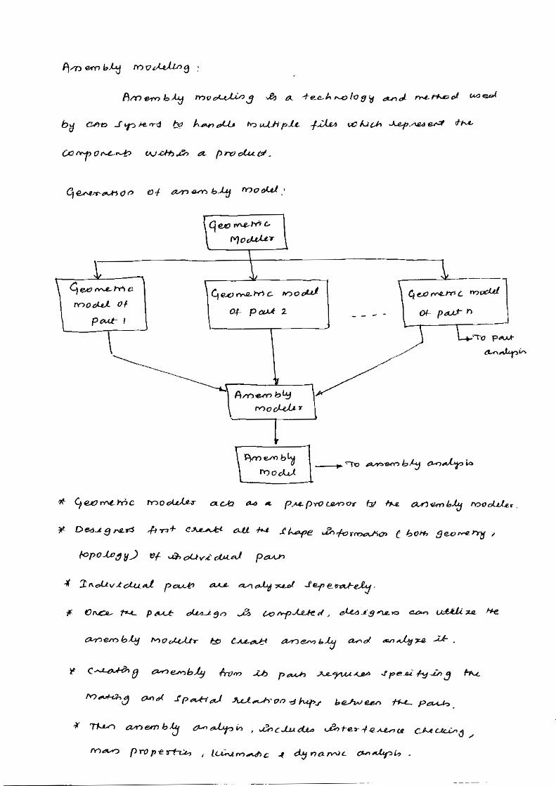
Assembly modeling is a technique applied by CAD and product visualization

software systems to utilize multiple files that shows components within a product. The

components within an assembly are called as solid / surface models.

The designer usually has approach to models that others are functioning on

concurrently. For example, different people may be creating one machine that has

different components. New parts are extra to an assembly model as they are generated.

Every designer has approach to the assembly model, during a work in progress, and while

working in their own components. The design development is noticeable to everyone

participated. Based on the system, it might be essential for the users to obtain the most

recent versions saved of every individual component to update the assembly.

The personal data files defining the 3D geometry of personal components are

assembled together via a number of sub assembly levels to generate an assembly

explaining the complete product. Every CAD methods support the bottom-up

construction. A few systems, through associative copying of geometry between

components allow top-down construction. Components can be situated within the

assembly applying absolute coordinate position methods.

Mating conditions are defines of the relative location of mechanism between each

other; for example axis position of two holes or distance between two faces. The final

place of all objects based on these relationships is computing using a geometry constraint

engine built into the CAD package.

The significance of assembly modeling in obtaining the full advantages of Product

Life-cycle Management has directed to ongoing benefits in this technology. These contain

the benefit of lightweight data structures that accept visualization of and interaction with

huge amounts of data related to product, interface between PDM systems and active

digital mock up method that combine the skill to visualize the assembly mock up with the

skill to design and redesign with measure, analyze and simulate.

2. Explain in detail, bottom up and top-down assembly approach.

Bottom up Assembly design In a ‘bottom up’ assembly design, complex assemblies are divided into minor

subassemblies and parts. Every part is considered as individual part by one or more designers.

The parts can be archived in a library in one or more 3D Files. This is the high effective way to

generate and manage complex assemblies.

Every part is included into the active part making a component request and thus an

assembly. The component will be the child of the active part and then it will be the active part.

Hence an instance of the actual part is applied; it revises automatically if the archived part is

edited by activating.

Bottom up Hierarchy:

The ‘bottom up’ assembly design hierarchy of the basic assembly is shown in figure . All

the parts exist prior to Part1. When Part1 is generated, it becomes the active. It would utilize

the menu sequence to add Bracket and it becomes the active part.

Insert > Component

Or

Assembly Design Tool Bar >

Top down Assembly Design

In a ‘top down’ assembly design all parts are classically designed by the similar

person within a single part. 3D assembly handles ‘top down’ method by allowing to design

and creation of a component while work in the active part. Hence, the active part will be

an assembly part.

The part becomes a child of the active part and then it will be the active part. The

part, when generated, is an instance of a base part which will be a root object located in

the active file. Every part is activated and modified as needed. The ‘top down’ assembly

design has its benefits. If the project is terminated or to go in a different new direction,

removing the file will remove the part and all of its components.

3. Explain in detail, the interference position and orientation

Interference of position and orientation Designers and manufacturers should check jointly that a provided product can be

assembled, without interference between parts, before the product to be manufactured.

Similarly, all the CAD tools presently have the potential to directly analyze the possibility of a

specified assembly plan for a product.

An assessment of previous assembly sequence and optimization research explains that

most previous assembly planners apply either feature-mating or interference-free techniques

to find assembly part interference interaction. In both feature-mating and interference-free

techniques focused upon the basic geometrical data and restrictions for the designed product,

which are generally contained in connected CAD files.

When completely automate the procedure of creating a professional assembly plan,

geometrical information for CAD models should be automatically taken from CAD files,

analyzed for interference relationships between components in the assembly, and then

designed for utilized the assembly analysis tools. Most of the previous assembly sequence

planners do not have the potential to complete the three tasks; they need users to manually

input part attributes or interference data, which is so time-consuming.

Determining Interference Relationships between Parts

In automated assembly schemes, most parts are assembled along with the principal

axis. Hence, to fine interference between parts while assembly, the projected technique

referred six assembly directions along with the principal assembly axis: +x, -x, +y, -y, +z, and -z.

But, the method could be improved, to think other assembly directions, as required. The

projected system uses projection of part coordinates onto planes in three principal axis (x, y ,z)

to find the obstruction between parts sliding along some of the six principal assembly axis. The

projections overlap between any two parts in a specified axis direction shows a potential

interference between the two parts, when one of the two parts slides along the specified

direction, with respect to the other. Vertex coordinates for overlapped

projections are then evaluated to find if real collisions would happen between parts with

overlapped projections. The planned process stores the determined interference data for

allocated assembly direction in a group of interference free matrices, for compatibility with

previous planners of assembly.

The swept volume interference and the multiple interference detection systems are

appropriate for three-dimensional interference determination between B-REP entities. But,

both techniques were developed for real-time interference detection between two moving

parts in a simulation environment. As a result, these two techniques are expensive in

computationally. For the assembly planning issue, actual collision finding capacity along

subjective relative motion vectors is not require. Instead, a efficient computational technique

is required for finding if two parts will collide when they are assembled in a specified order

along any one of the six principle assembly axis.

4. Explain in detail, tolerance stack-up

Tolerance stack-up

Tolerance stack-up computations show the collective effect of part tolerance with

respect to an assembly need. The tolerances ‘stacking up’ would describe to adding tolerances

to obtain total part tolerance, then evaluating that to the existing gap in order to see if the

design will work suitably. This simple evaluation is also defined as ‘worst case analyses’. Worst

case analysis is suitable for definite needs where failure would signify failure for a company. It

is also needful and suitable for problems that occupy a low number of parts. Worst case

analysis is always carried out in a single direction that is a 1-D analysis. If the analysis has part

dimensions that are not parallel to the assembly measurement being defined, the stack-up

approach must be edited since 2D variation such as angles, or any variation that is not parallel

with the 1-D direction, does not influence the measurement of assembly with a 1-to-1 ratio.

The tolerance stacking issue occurs in the perception of assemblies from

interchangeable parts because of the inability to create or join parts accurately according to

nominal. Either the applicable part dimension changes around various nominal value from

part by part or it is the act of assembly that directs to variation. For example, as two parts are

combined through matching holes pair there is not only variation in the location of the holes

relative to nominal centers on the parts but also the slippage difference of matching holes

relative to each other when safe.

Thus there is the opportunity that the assembly of such interacting parts will not move

or won’t come closer as planned. This can generally be judged by different assembly criteria,

say G1, G2,... Here we will be discussed with just one assembly criterion, say G, which can be

noted as a function of the part dimensions L1,...,Ln. A example is shown in Figure 4.7., where n

= 6 and is the clearance gap of interest. It finds whether the stack of cogwheels will locate

within the case or not. Thus it is preferred to have G > 0, but for performance of functional

causes one may also require to limit G.

G = L1 − (L2 + L3 + L4 + L5 + L6)

= L1 − L2 − L3 − L4 − L5 − L6

Fig. Tolerance Stack-up

As per the example, the required lengths ‘Li ‘may vary from the nominal lengths ‘λi’ by

a small value. If there is higher variation in the ‘Li’ there may well be important problems in

accepting G > 0. Thus it is sensible to limit these changes via tolerances. For similar tolerances,

‘Ti’, represent an ‘upper limit’ on the absolute variation between actual and nominal values of

the i th detail part dimension, it is means that |Li − λi| ≤ Ti. It is mostly in the interpretation of

this last inequality that the different methods of tolerance stacking vary. The nominal value ‘γ’of G is typically computed by replacing in equation L1 − L2 − L3 − L4 − L5 −

L6, the actual values of Li’s by the corresponding nominal values of λi, that is γ = λ1 − λ2 − λ3 −

λ4 − λ5 − λ 6.

5. Write short notes on statistical method for tolerance analysis.

Statistical method for tolerance analysis (RSS) :

In RSS method, tolerance stacking a significant new element is added to the

assumptions, specifically which the detail differences from nominal are random and

independent from part by part. It is expensive in the sense that it frequently commanded very

close tolerances. That all variations from nominal should dispose themselves in worst case

method to defer the higher assembly tolerance is a relatively unlikely proposition. On the

other hand, it had the advantage of assurance the resulting assembly tolerance. Statistical

tolerance in its typical form operates under two basic hypotheses:

As per Centered Normal Distribution, somewhat considering that the ‘Li’ can occur

anywhere within the tolerance distribution *λi − Ti, λi + Ti+, assume that the ‘Li’ are normal

random variables, that is change randomly according to a normal distribution, centered on

that similar interval and with a ±3σ distribute equal to the span of that interval, hence 99.73%

of all ‘Li’ values occur within this gap. As per the normal distribution is such that the ‘Li’ fall

with upper frequency in the middle near ‘λi’ and with low frequency closer the interval

endpoints. The match of the ±3σ distribution with the span of the detail tolerance span is

hypothetical to state that almost all parts will satisfy the detail tolerance limits as shown in

figure .

Fig. Centered Normal Distribution Statistical tolerance stacking formula is given below:

Where, ai = ±1 for all i = 1,...,n.

Typically Tstat assy is considerably smaller than T arith assy. For n=3, the scale of this variation

is simply visualized and valued by a rectangular box with side lengths T1, T2 and T3. To obtain

from one corner of the box to the diagonally opposite corner, one can cross the gap T21 + T22 +

T23 along that diagonal and follow the three edges with lengths T1, T2, and T3 for a total length

T= T1 + T2 +T3 as shown in figure .

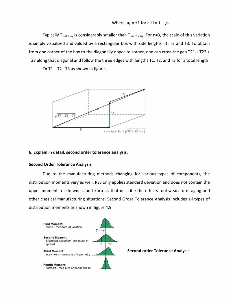
6. Explain in detail, second order tolerance analysis.

Second Order Tolerance Analysis

Due to the manufacturing methods changing for various types of components, the

distribution moments vary as well. RSS only applies standard deviation and does not contain the

upper moments of skewness and kurtosis that describe the effects tool wear, form aging and

other classical manufacturing situations. Second Order Tolerance Analysis includes all types of

distribution moments as shown in figure 4.9

Second order Tolerance Analysis

Second Order Tolerance Analysis is required to find what output is going to be when the

assembly function is not linear. In classical mechanical engineering developments kinematic

changes and other assembly performances result in non-linear assembly operations. Second

order estimates are more complex so manual calculations are not suitable but the computation

is greatly improved and becomes feasible within tolerance analysis software.

7. Write the importance, advantages and limitations of tolerance analysis.

Importance of Tolerance Analysis

With smaller product lifecycles, quicker to market, and higher cost pressures, the

uniqueness that distinguishes a product from its competitors. Engineers are moving to the next

order of resolution in order to improve cycle time and quality and to reduce costs. They are

showing nearer at why they did not get the correct part and assembly dimension values they

needed from manufacturing and then are trying to optimize the tolerances on the following

version of the product. Optimization of tolerance during design has a high impact on the output

of manufacturing, and better yields direct impact on product cost and quality. Tolerance

Analysis before trying to manufacture a product helps engineers avoid time taking iterations

later in the design cycle.

The electronics industry is attaining customer satisfaction purposes via a physical

shrinking of their components while adding more capabilities. As electronic devices high densely

packaged, the significance increases to more accurately understanding the interaction of

manufacturing variation and tolerances in design. Similarly, in the aircraft, automotive and

medical device productions, liability costs are increasing while environmental needs are being

more forcefully forced such that companies requires to understand high precisely what may

reason a failure.

Advantages of Tolerance Analysis 1. Accurate part assembly. 2. Elimination of assembly rework 3. Improvement in assembly quality. 4. Reduction of assembly cost. 5. High customer satisfaction. 6. Effectiveness of out-sourcing.

Limitations of Tolerance Analysis 1. Time consuming process. 2. Skill require for complex assemblies.

8. Explain in detail, mass property calculations.

Mass property calculations

The first step in finding mass properties is to set up the location of the X, Y, and Z axis.

The correctness of the calculations will depend completely on the knowledge used in choosing

the axis. Hypothetically, these axes can be at any position relative to the object being

considered, offered the axes are equally perpendicular. But, in reality, except the axes are

chosen to be at a position that can be precisely measured and identified, the calculations are

meaningless.

Fig. Accuracy of axis – Vertical

As shown in the figure . the axes do not create a best reference hence a small error in

squareness of the base of the cylinder origins the object to tilt away from the vertical axis.

Fig. Accuracy of axis – Horizontal

An axis should always pass via a surface that is firmly linked with the bulk of the component. As

shown in the figure, it would be best to position the origin (Z=0) at the end of the component

rather than the fitting that is freely dimensioned virtual to the end.

Calculating Center of gravity location The center of gravity of an object is: described the ‘center of mass’ of the object. the location where the object would balance. the single point where the static balance moments are all zero about three mutually

perpendicular axis. the centroid of object the volume when the object is homogeneous. the point where the total mass of the component could be measured to be concentrated

while static calculations. the point about where the component rotates in free space the point via the gravity force can be considered to perform the point at which an exterior force must be used to create translation of an object in space

Center of gravity location is stated in units of length along the three axes (X, Y, and Z).

These three components of the vector distance from the base of the coordinate system to the

Center of gravity location. CG of composite masses is computed from moments considered

about the origin. The essential dimensions of moment are Force and Distance. On the other

hand, Mass moment may be utilized any units of Mass times Distance. For homogeneous

components, volume moments may also be considered. Care should be taken to be confident

that moments for all parts are defined in compatible units.

Component distances for CG position may be either positive or negative, and in reality

their polarity based on the reference axis position. The CG of a homogeneous component is

determined by determining the Centroid of its volume. In practical, the majority of components

are not homogeneous, so that the CG must be calculated by adding the offset moments along all

of the three axes.

Fig. Center of Gravity