MIMO Toolbox

For Use with MATLAB

Oskar Vivero

About the toolbox The MIMO Toolbox is a collection of MATLAB functions and a GUI. Its purpose is to complement the Control Toolbox for MATLAB with functions capable of handling the multivariable input-output scheme. All the results and examples except for example 1.1.2.1 were obtained with the MIMO Toolbox and were corroborated with the bibliography. April, 2006

Installation The installation is straightforward just copy the directory “Mimotools” and add the path to the MATLAB search path. See path, in the MATLAB documentation for more information.

Requirements The MIMO Toolbox was created in Matlab 7.1 (R14) SP3, and requires the Symbolic and Control Toolboxes.

Contact Oskar Vivero oskar.vivero@gmail.com

Contents 1. Theory behind the functions

1.1. SISO Systems 1.1.1. Feedback Basic Concepts 1.1.2. Nyquist’s Stability Criterion

1.2. MIMO Systems 1.2.1. Poles and Zeros of a MIMO System

1.2.1.1. Smith-McMillan Transformation 1.2.2. Stability of MIMO Systems

1.2.2.1. Generalized Nyquist’s Stability Criterion 1.2.3. Treating a MIMO System with SISO techniques

1.2.3.1. Coupling degree and pairings of inputs and outputs 1.2.3.2. Nyquist’s Arrays and Gershgorin Bands 1.2.3.3. Relative Gain Array (RGA) 1.2.3.4. Individual Channel Design (ICD)

2. Function Reference

2.1. The Symbolic Transfer Function 2.2. Function Description

2.2.1. tf2sym 2.2.2. sym2tf 2.2.3. ss2sym 2.2.4. smform 2.2.5. rga 2.2.6. nyqmimo 2.2.7. m_circles 2.2.8. icdtool 2.2.9. gershband 2.2.10. arrowh

3. References

1 1 1 2 4 4 4 7 7

10 10 10 11 12

14 14 14 14 15 16 16 17 17 19 19 20 21

22

MIMO Toolbox

- 1 -

1. Theory behind the functions The aim of this chapter is to introduce the MIMO control theories so that one can understand both, the algorithm behind each function and its proper use. This chapter is only intended to provide a brief description of such theories and it’s recommended that the user refers to the bibliography listed at the end of this document.

1.1 SISO Systems 1.1.1 Feedback Basic Concepts Assuming a lineal process that is time-invariant whose behavior is defined by lineal differential equations with constant coefficients:

1 2 1 2y a y a y b u b u•• • •

+ + = +

where ( )y t is the output signal and ( )u t is the input signal, its possible to obtain a

transfer function by applying the Laplace’s Transform

( )( ) ( ) ( )

( )1 2

21 2

Y s N s b s bG s

U s D s s a s a+

= = =+ +

( )( )

If 0 then is defined as a zero.

If then is defined as a pole.Z Z Z

P P P

s s G s s

s s G s s

= � =

= � = ∞

If ( )G s is rational, usually ( )D s determines the dynamic characteristics of the system,

unless there exist cancellations between ( )N s and ( )D s .

Let ( )H s and ( )G s be two transfer functions

The stability of the system in a closed-loop configuration is given by ( ) ( )1 G s H s+ if

and only if there is no cancellation of instabilities. For any design, it’s possible to verify its stability by finding the singularities of ( )CLG s . If any of the singularities is

located in 2+� or near the imaginary axis, it’s almost impossible to determine the modifications needed on either ( )G s or ( )H s to avoid the location of the singularities.

The Nyquist’s stability criterion provides a tool for solving the problem

( ) ( )( ) ( )1CL

G sG s

G s H s=

+

MIMO Toolbox

- 2 -

1.1.2 Nyquist’s Stability Criterion The system in a closed-loop configuration is stable if and only if the trajectory of the Nyquist diagram of ( ) ( )G j H jω ω from ω−∞ < < ∞ surrounds the point ( )1,0− in a

counter-clockwise direction as much times as ( ) ( )G s H s has unstable poles.

Theorem – suppose that a function ( )f z is meromorphic in a simply connected domain

D, and that C is a simple closed positively oriented contour in D such that ( )f z does

not contain any singularities. Then

( )( )'1

2 f f

f zN dz Z P

i f zπ= = −��

where N is the winding number, fZ is the number of zeros inside the contour and fP

is the number of poles inside the contour.

Example 1.1.2.1 The image of the circle of radius 2 centered at the origin under ( ) 2f z z z= + is the

curve ( ) ( ) ( ) ( ) ( )( ), 4cos 2 2cos , 4sin 2 2sing x y t t t t= + + . Note that the curve ( ),g x y

winds up twice around the origin. We check this by computing

( )( )

0 1

0 1

2 2

'1 ; Singulatiries at 0 and 1

2

2 1 2 1Res Res 2

C

z z

f zN z z

i f z

z zN

z z z z

π= = = −

+ +� � � �= + =� � � �+ +� � � �

�

Having defined N , it’s important to define a useful contour for the stability analysis. It’s possible to know from the root locus analysis and the time response that the unstable poles are at the right side of the S-plane. Since the zeros of the open loop system are the poles of the closed loop system, we’ll focus on finding the unstable zeros through Nyquist frequency analysis. The contours that we’ll consider are:

MIMO Toolbox

- 3 -

Example 1.1.2.2 – [4] pp. 620

Draw the Nyquist contour and diagram of ( ) ( )( )( )500

1 3 10G s

s s s=

+ + +

Once the stability of a system has been defined through the Nyquist’s diagram, the robustness of the system can be defined by two quantities, the gain and phase margins. Gain margin ( )MG - the change of gain in open loop needed to obtain a phase shift at

180° that turns the system unstable. Phase margin ( )MΦ - the phase shift in open loop needed to turn the system unstable

with a unit gain.

MIMO Toolbox

- 4 -

1.2 MIMO Systems The basic description of a multivariable system is through a transfer function matrix (TFM), whose elements ,i jg represent the i-est output with the j-est input. The

elements ,i jg are individual transfer functions.

1.2.1 Poles and zeros of a MIMO system The poles and zeros of multivariable systems can be defined in several (not all equivalent) ways, but the definitions that yield the most significant consequences are given by [1]: The zeros of a transfer function matrix ( )H s , are the roots of the (nonzero) numerator

polynomials ( ){ }i sε in the Smith-McMillan form of ( )H s . The Smith-McMillan form

allows us to give a physical interpretation of the zeros. If Zs is a zero, then the Smith-

McMillan form of ( )H s will lose rank at Zs s= .

The poles of a transfer function matrix ( )H s , are the roots of the denominator

polynomials in the Smith-McMillan form of ( )H s .

1.2.1.1 Smith – McMillan Transformation Given a rational matrix ( )H s

( ) ( )( )

N sH s

d s=

where ( )d s is the monic least common multiple of the denominators of ( )H s

Then ( ) ( ) ( )d s H s N s= is a polynomial matrix, so that we can write,

( ) ( ) ( ) ( ) ( ) ( )1 2d s H s N s U s s U s= = Λ

MIMO Toolbox

- 5 -

where the ( ){ }iU s are unimodular matrices and ( )sΛ is in Smith form

( ) ( ) ( ) ( )( )

( )( )

( )( )

( )( )

1 11 2

i

i i

i

s sU s H s U s diag

d s d s

s s

d s s

λ

λ εψ

− − Λ � �= = � � �� �

=

where ( ) ( ){ },i is sε ψ are coprime, 1, ,i r= �

and r is the (normal) rank of ( )H s

Then we can write

( ) ( ) ( ) ( )1 2H s U s M s U s=

where ( )M s is the Smith-McMillan transformation of ( )H s given by

( )( )( )

0

0 0

i

i

sdiag

M s s

εψ

� � � �� �� = � �� �� �� �� �

Smith Form For any p m× polynomial matrix ( )P s we can find elementary row and column

operations, or corresponding unimodular matrices ( ) ( ){ },U s V s such that

( ) ( ) ( ) ( )U s P s V s s= Λ

where

( )

( )

( )

( )

0

00 0 0

the (normal) rank of

i

r

s

ss

r P s

λ

λ

� �� �� �Λ =� �� �� �

=

� �

�

and the ( ){ }i sλ are unique monic polynomials obeying a division property

( ) ( )1 , 1, , 1i is s i rλ λ + = −�

Moreover, if ( ) ( ) the gcd of all minors of i s i i P s∆ = ×

then

( ) ( )( ) ( )0

1

, 1ii

i

ss s

sλ

−

∆= ∆ =

∆

The matrix ( )sΛ is called the Smith form of ( )P s

MIMO Toolbox

- 6 -

Example.1.2.1.1 – [1] pp. 444-446 Find the poles and zeros of

( )( ) ( )

( )( ) ( )

2

2 2 2 2

11

1 2 1 1

s s sG s

s s s s s s

� �+� �=� �+ + − + − +� �

Solution Given

( ) ( ) ( )1G s N s

d s=

where

( ) ( ) ( ){ } ( ) ( )

( ) ( )( ) ( )

2 2 2 2

2

2 2

1 2 1 2

1

1 1

d s lcm s s s s

s s sN s

s s s s

= + + = + +

� �+� �=� �− + − +� �

Finding ( )sΛ in Smith form:

( )( ) ( ) ( ) ( )( )

( ) ( ) ( )( )( ) ( )

( ) ( ) ( ) ( )

0

2 2 21

232

1 1

222 2

1

gcd , 1 , 1 , 1

gcd 1 2

1 2

s

s s s s s s s s s

s s s s

s s s

s s s s s

ε λ

ε λ

∆ =

∆ = + − + − + =

∆ = + +

= =

= = + +

Therefore

( )( )( ) ( ) ( )2 2

2

00 1 2

00 02

i

i

ss

diag s sM s s

ss

εψ

� �� � � � � �+ +� �� � �= =� �� �� � � �� � � �� � +� �

The poles are defined as

( ) ( ) ( ) ( ) ( ) ( )[ ]

2 21 2 1 2 2 0

1 1 2 2 2

p s s s s s s

p

ψ ψ= ⋅ = + + ⋅ + =

= − − − − −

The zeros are defined as

( ) ( ) ( )[ ]

31 2 0

0 0 0

z s s s s

z

ε ε= ⋅ = =

=

MIMO Toolbox

- 7 -

1.2.2 Stability of MIMO Systems Having defined a tool in order to obtain the poles and zeros of a MIMO system, it’s necessary to define if the system is stable. This can be achieved by the generalized Nyquist’s stability criterion, which is an adaptation from the Nyquist’s stability criterion for SISO systems. 1.2.2.1 Generalized Nyquist’s Stability Criterion Let ( )G s be a rational TFM, assuming that it has no cancellations between poles and

zeros. Let K be a compensator with a negative feedback loop, that is

I ; K k k= ∈�

Let the ( )det I KG s+� �� � have P poles and Z zeros in the right hand plane (RHP), then

like in SISO systems

( ) ( )arg det I 2KG s Z Pπ∆ + = − −� �� �

where arg∆ is the change of phase given by s along the Nyquist’s contour. In order to obtain stability in a closed loop, it is required that the diagram mapped by

( )det I KG s+� �� � surrounds the origin P times.

As a difference from the SISO case, the Nyquist diagram of each k of interest must be obtained. If ( )i sλ is an eigenvalue of ( )G s , then ( )ik sλ is an eigenvalue of ( )KG s , and

therefore, ( )1 ik sλ+ is an eigenvalue of ( )I KG s+ . Then

( ) ( )det I 1 i

i

KG s k sλ+ = +� � � �� � � �∏

and

( ) ( )arg det I arg 1 i

i

KG s k sλ∆ + = ∆ +� � � �� � � ��

Therefore, the stability in a closed loop system can be inferred by the number of wind ups to the point ( )1,0− given by the Nyquist diagram of ( )ik sλ . The Nyquist diagram

of ( )i sλ are known as the characteristic graphs of ( )G s .

MIMO Toolbox

- 8 -

Theorem – If ( )G s has right hand plane poles (RHPP), P, given by the Smith-McMillan

transformation, then the closed loop with negative feedback is stable if and only if the characteristic graphs of ( )KG s surround the point ( )1,0− P times in a counter-

clockwise direction, assuming that there was no cancellations of instabilities. Example 1.2.2.1 – [2] pp. 61 Find the values of 0k > in order to keep ( )G s from becoming unstable

( ) ( )( )11

6 21.25 1 2

s sG s

ss s

−� �= � �− −+ + � �

Solution It’s easy to verify that the open loop poles of ( )G s are [ ]1 2P = − − , therefore, in

order to maintain the closed loop system stable, we must ensure that the number of surroundings of the characteristic graphs of ( )G s is equal to zero.

Assuming 1k = , then ( )

( )( )

( )( )

2

1

2

2

det I 0

2 2 3 24 1

5 3 2

2 2 3 24 1

5 3 2

KG s

s s

s s

s s

s s

λ

λλ

Λ = − =� �� �

� �− + − +� �� �+ +� � � �Λ = =� � � �� � − − − +� �� �+ +� �

From the eigenvalues of ( )G s , its possible to obtain the Generalized Nyquist Diagram

when 1k =

MIMO Toolbox

- 9 -

From the diagram it’s possible to obtain the critical points in which we can calculate the values of k , in order to keep the system stable. Knowing that the critical points are in

0.8− and 0.4− , therefore

1 11.25 , 2.5

0.8 0.4k k� � � �< = > =� � � �

� � � �

This can be proven by setting the values of k equal to 1.25 and 2.5 and obtaining the Nyquist Diagram.

MIMO Toolbox

- 10 -

1.2.3 Treating a MIMO system with SISO techniques 1.2.3.1 Coupling degree and pairing of inputs and outputs Given the coupling degree of a MIMO system, it’s possible to apply certain SISO techniques for designing controllers. The degree of coupling can be found by several techniques, such as the Nyquist’s arrays and the Gershgorin bands, the relative gain array (RGA), and the individual channel design (ICD). In some cases, it is possible to cross couple inputs and outputs in order to obtain a less coupled system. 1.2.3.2 Nyquist’s Arrays and Gershgorin bands The Nyquist’s array of a TFM ( )G s , is an array of graphs, where the i, j-est graph is the

Nyquist Diagram of ,i jg .

Gershgorin Theorem – let Z a n n× complex matrix. Then, the eigenvalues of Z fall on the union of circles with center at ,i iz with radius

,1

m

i jj

j i

Z=≠

�

and on the circles with center at ,j jz with radius

,1

m

i ji

i j

Z=≠

�

Gershgorin Bands Over the Nyquist’s diagram of ( ),i ig s , on each point, we super impose a circle of

radius

( ) ( ), ,1 1

or m m

i j j ii i

i j i j

g j g jω ω= =≠ ≠

� �

The bands obtained in this way are known as the Gershgorin Bands. By the Gershgorin theorem it’s possible to know that the bands trap the unions of the Nyquist diagram. More over, it’s possible to demonstrate that the bands occupy different regions, therefore there will be as many Nyquist’s diagrams trapped in a region as many Gershgorin bands are there. Then, by counting the number of wind ups that the Gershgorin bands do around the point ( )1,0− , its possible to determine the stability of the MIMO system.

MIMO Toolbox

- 11 -

If the Gershgorin bands are thin and exclude the origin, it is said that ( )G s is

diagonally dominant which can be interpreted as a decoupled system. Example 1.2.3.1– [3] pp. 657 Find the Gershgorin bands of

( )2

2 2

2 0.113 2

0.1 62 1 5 6

ss sG s

s s s s

� �� �++ += � �� �� �+ + + +� �

From the graphs above, it’s possible to observe that the system is stable and highly decoupled. Therefore, it can be managed as two independent SISO systems with small disturbances due to the small coupling degree. 1.2.3.3 Relative Gain Array (RGA) To measure the degree of coupling or interaction in a system, the concept of relative gain array can be used. For an arbitrary n n× matrix A, it is defined as

( ) ( )1RGA .*T

A A A−=

The RGA matrix has a number of interesting properties

• The sum of the elements of any row or column is always 1 • RGA is independent of any scaling • The sum of the absolute values of all elements in ( )RGA A is a good measure of

A’s true condition number, i.e., the best condition number that can be achieved in the family 1 2D AD , where iD are diagonal matrices.

• Permutation of the rows or columns of A leads to permutations of the corresponding rows or columns of ( )RGA A .

MIMO Toolbox

- 12 -

Clearly RGA of a diagonal matrix is the unit matrix. The deviation of RGA from the unit matrix can be taken as a measure of the coupling degree between y Ax= . For a n m× matrix, the RGA is defined as

( ) ( )†RGA .*T

A A A=

where †A denotes the pseudo inverse of A. Example 1.2.3.2– [3] pp. 657 Let ( )G s be

( )2

2 2

2 0.113 2

0.1 62 1 5 6

ss sG s

s s s s

� �� �++ += � �� �� �+ + + +� �

( )( ) 1.0101 0.0101RGA

0.0101 1.0101G S

−� �= � �−� �

Since ( )( )RGA IG S → , it’s possible to observe that the system is highly decoupled.

This corroborates the result given by the Gershgorin bands in example 1.2.3.1. 1.2.3.4 Individual Channel Design (ICD) As a difference from RGA and the Gershgorin Bands which are useful tools for calculating the cross-coupling of a system, the Individual Channel Design is a framework in which Bode/Nyquist techniques can be applied directly to the channels not only when cross-coupling is weak but in all circumstances, including when cross-coupling is strong. The multivariable system is decomposed into an equivalent set of SISO systems. Each SISO system is the open-loop channel transmittance between output ( )iY s and input ( )iR s with all internal loops closed. [6]

Let ( )G s be a 2 2× system with a controller of the type ( ) ( )iK s diag k s= � �� � then the

relationships of ( )( )

i

i

Y s

R s can be established as

( )( ) ( )

( )( ) ( )

11 1 11 2

1

22 2 22 1

2

1

1

Y sC k g h

R s

Y sC k g h

R s

γ

γ

= = −

= = −

where ( )iC s is the individual channel, ( )sγ is the multivariable structure function

(MSF) and ( )ih s is the subsystem i, which are respectively defined as:

MIMO Toolbox

- 13 -

( )

( )

12 21

11 22

1i ii

ii ii

g gs

g g

k gh s

k g

γ =

=+

The MSF ( )sγ is of great importance inside the ICD analysis framework, since it is

capable of [6]

• Determining the dynamical characteristics between each input and each output • It has an interpretation in the frequency domain • Its magnitude quantifies the amount of coupling between the channels • It can determine the transmittance zeros of the system from ( )1 sγ−

• ( ) 1sγ = determines the non-minimum phase conditions

• Its closeness to the point ( )1,0 it’s a key point in determining the robustness of

the system Robustness Conditions In order to obtain a design that provides a channel that is robust and stable, the following conditions should be satisfied

1. ( )sγ should not be close to the point ( )1,0 for all ω

2. ( ) ( )is h sγ shall be robust

3. ( ) ( )i iik s g s shall be robust

The interaction between the discarded inputs and outputs can be observed from

( ) ( )( ) ( ) ( ) ( )1

1ij

i j jjj i

g sY s h s R s

g s C s= ⋅ ⋅

+

MIMO Toolbox

- 14 -

2. Function Reference The aim of this chapter is to give a brief description of the functions used in the MIMO toolbox. For the users that are new to the Matlab environment it is recommended to review the getting started documentation.

2.1 The Symbolic Transfer Function The Control Toolbox in Matlab posses an object class that describes a transfer function. This model representation is numerical and it’s sensitive to floating point errors due to arithmetic operations such as inversion. Also, from the LTI definition, the transfer function class cannot handle nonlinearities such as square roots, trigonometric functions, etc, since it’s only a rate in polynomial representation. Given such problems, a symbolic conversion for transfer function has been developed, and it’s key to some of the functions inside the MIMO toolbox. This conversion enables the user to handle the transfer function and its operations as an algebraic problem, simplifying the computational difficulties that may arise for the users without a computer science background.

2.2 Function Description 2.2.1 tf2sym Syntax G_sym = tf2sym(G) Description tf2sym performs the conversion from a numeric to a symbolic representation of a transfer function. The function is capable to deal with both SISO and MIMO models. To be able to differentiate the type of transfer function, the symbolic transfer function is represented with the Laplace operator ‘p’ instead of ‘s’.

Example 1 >> G=tf([1 2 3],[1 5 6 7]) >> G_sym=tf2sym(G); >> pretty(G_sym) 2 3 + p + 2 p ------------------- 3 2 p + 5 p + 6 p + 7

Example 2 >> g11=tf([1 2],[1 2 1]); g12=tf([1 -1],[1 5 6]); g21=tf([1 -1],[1 3 2]); g22=tf([1 2],[1 1]); G=[g11 g12; g21 g22]; g=tf2sym(G); pretty(g)

MIMO Toolbox

- 15 -

[ 2 + p -1 + p ] [ -------- ---------------] [ 2 (p + 3) (2 + p)] [ (p + 1) ] [ ] [ -1 + p 2 + p ] [--------------- ----- ] [(2 + p) (p + 1) p + 1 ] 2.2.2 sym2tf Syntax G = sym2tf(G_sym)

Description sym2tf performs the conversion from a symbolic to a numeric representation of a transfer function. As tf2sym, this function is capable of dealing with both SISO and MIMO models. This conversion cannot handle nonlinearities since the numeric transfer function class ‘tf’ is not capable of dealing with the nonlinearities. Example 1 >> syms p >> G_sym = (p^2 + 2*p + 3)/(p^3 + 5*p^2 + 6*p + 7); >> G=sym2tf(G_sym) Transfer function: s^2 + 2 s + 3 --------------------- s^3 + 5 s^2 + 6 s + 7

Example 2 >> g11=(p + 2)/(p^2 + 2*p + 1); g12=(p - 1)/(p^2 + 5*p + 6); g21=(p - 1)/(p^2 + 3*p + 2); g22=(p + 2)/(p + 1); g=[g11 g12; g21 g22]; G=sym2tf(g) Transfer function from input 1 to output... s + 2 #1: ------------- s^2 + 2 s + 1 s - 1 #2: ------------- s^2 + 3 s + 2 Transfer function from input 2 to output... s - 1 #1: ------------- s^2 + 5 s + 6 s + 2 #2: ----- s + 1

MIMO Toolbox

- 16 -

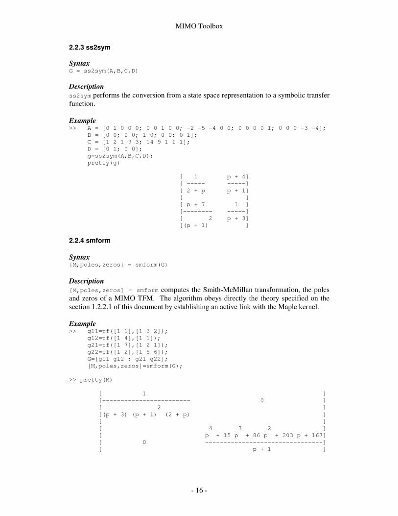
2.2.3 ss2sym Syntax G = ss2sym(A,B,C,D) Description ss2sym performs the conversion from a state space representation to a symbolic transfer function. Example >> A = [0 1 0 0 0; 0 0 1 0 0; -2 -5 -4 0 0; 0 0 0 0 1; 0 0 0 -3 -4]; B = [0 0; 0 0; 1 0; 0 0; 0 1]; C = [1 2 1 9 3; 14 9 1 1 1]; D = [0 1; 0 0]; g=ss2sym(A,B,C,D); pretty(g) [ 1 p + 4] [ ----- -----] [ 2 + p p + 1] [ ] [ p + 7 1 ] [-------- -----] [ 2 p + 3] [(p + 1) ] 2.2.4 smform Syntax [M,poles,zeros] = smform(G)

Description [M,poles,zeros] = smform computes the Smith-McMillan transformation, the poles and zeros of a MIMO TFM. The algorithm obeys directly the theory specified on the section 1.2.2.1 of this document by establishing an active link with the Maple kernel. Example >> g11=tf([1 1],[1 3 2]); g12=tf([1 4],[1 1]); g21=tf([1 7],[1 2 1]); g22=tf([1 2],[1 5 6]); G=[g11 g12 ; g21 g22]; [M,poles,zeros]=smform(G); >> pretty(M) [ 1 ] [------------------------ 0 ] [ 2 ] [(p + 3) (p + 1) (2 + p) ] [ ] [ 4 3 2 ] [ p + 15 p + 86 p + 203 p + 167] [ 0 --------------------------------] [ p + 1 ]

MIMO Toolbox

- 17 -

>> poles poles = -3.0000 -2.0000 -1.0000 -1.0000 + 0.0000i -1.0000 - 0.0000i >> zeros zeros = -5.3101 + 2.5439i -5.3101 - 2.5439i -2.1899 + 0.1460i -2.1899 - 0.1460i

2.2.5 rga Syntax A=rga(G)

Description rga computes the Relative Gain Array of a MIMO TFM. The algorithm obeys directly the theory specified on the section 1.2.3.3 Example >> g11=tf([1 2],[1 2 1]); g12=tf([1 -1],[1 5 6]); g21=tf([1 -1],[1 3 2]); g22=tf([1 2],[1 1]); G=[g11 g12; g21 g22]; A=rga(G) A = 1.0213 -0.0213 -0.0213 1.0213

2.2.6 nyqmimo Syntax nyqmimo(G)

Description nyqmimo computes the Nyquist’s Diagram based on the type of transfer function at the input. nyqmimo distinguishes between transfer functions with singularities at the origin, proper, strictly proper and strictly improper transfer functions, based on that structure, it maps the Nyquist’s Diagram according to the Nyquist’s Contour. nyqmimo is capable of computing the Nyquist’s Diagram for SISO and the Generalized Nyquist’s Diagram for MIMO systems.

MIMO Toolbox

- 18 -

Example 1 >> G=tf([1 25],[1 5 3 -9 0]); nyqmimo(G)

Example 2 >> den=1.25*conv([1 1],[1 2]); g11=tf([1 -1],den); g12=tf([1 0],den); g21=tf([-6],den); g22=tf([1 -2],den); G=[g11 g12;g21 g22]; nyqmimo(G)

2.2.7 m_circles Syntax m_circles

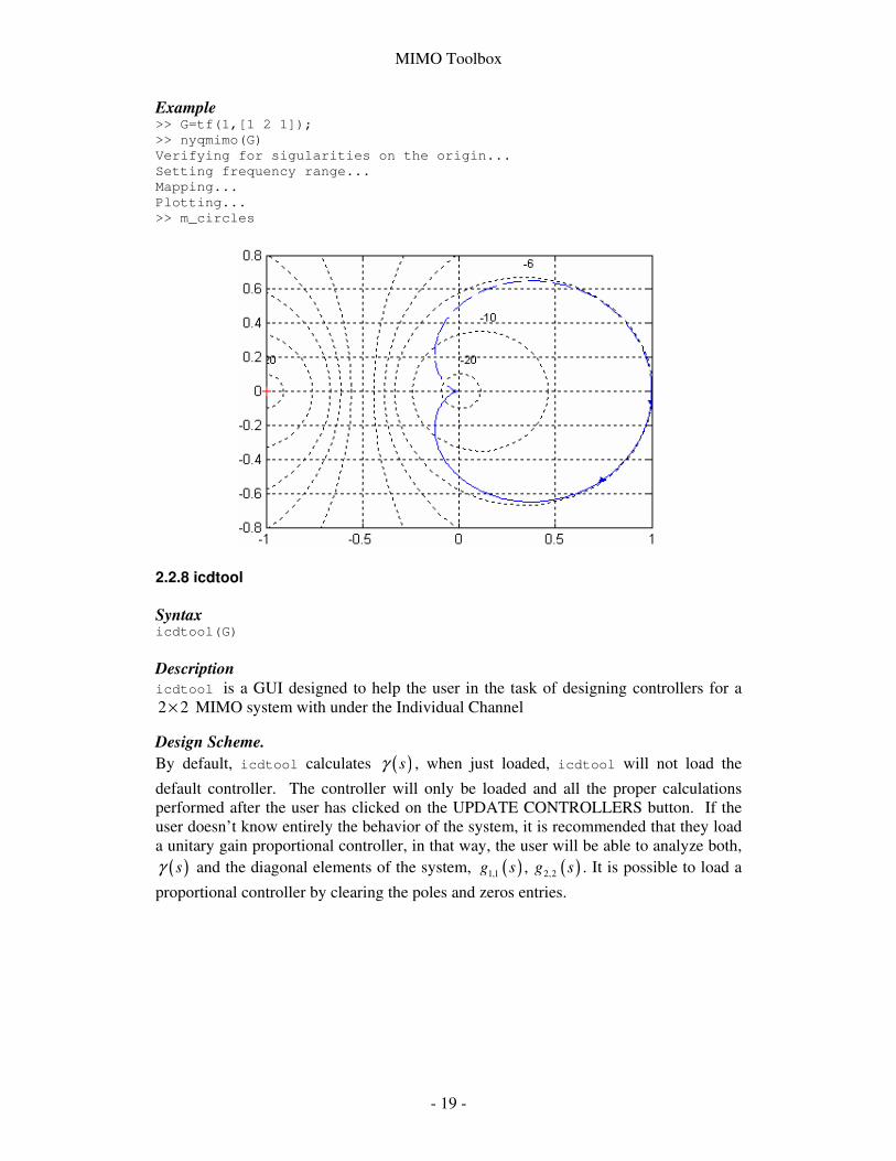
Description m_circles superimposes the M circles of magnitude -2dB to 20dB. This function is useful to measure the gain margin on a Nyquist’s Diagram.

MIMO Toolbox

- 19 -

Example >> G=tf(1,[1 2 1]); >> nyqmimo(G) Verifying for sigularities on the origin... Setting frequency range... Mapping... Plotting... >> m_circles

2.2.8 icdtool Syntax icdtool(G)

Description icdtool is a GUI designed to help the user in the task of designing controllers for a 2 2× MIMO system with under the Individual Channel

Design Scheme. By default, icdtool calculates ( )sγ , when just loaded, icdtool will not load the

default controller. The controller will only be loaded and all the proper calculations performed after the user has clicked on the UPDATE CONTROLLERS button. If the user doesn’t know entirely the behavior of the system, it is recommended that they load a unitary gain proportional controller, in that way, the user will be able to analyze both,

( )sγ and the diagonal elements of the system, ( ) ( )1,1 2,2, g s g s . It is possible to load a

proportional controller by clearing the poles and zeros entries.

MIMO Toolbox

- 20 -

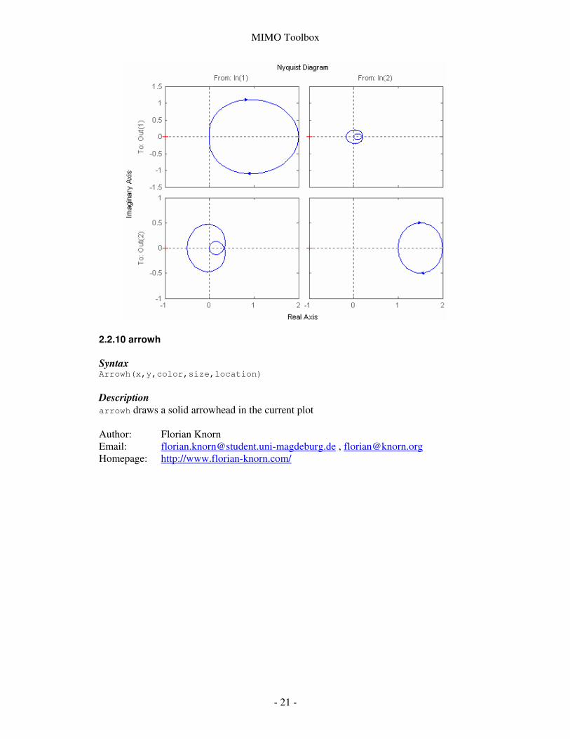
2.2.9 gershband Syntax gershband(G) – Gershgorin bands of G gershband(G,’v’) – Gershgorin bands and Nyquist Array of G

Description gershband computes the Gershgorin Bands of a n n× MIMO system along with the Nyquist’s Array. Example >> g11=tf([1 2],[1 2 1]); g12=tf([1 -1],[1 5 6]); g21=tf([1 -1],[1 3 2]); g22=tf([1 2],[1 1]); G=[g11 g12; g21 g22]; gershband(G,’v’);

MIMO Toolbox

- 21 -

2.2.10 arrowh Syntax Arrowh(x,y,color,size,location)

Description arrowh draws a solid arrowhead in the current plot Author: Florian Knorn Email: florian.knorn@student.uni-magdeburg.de , florian@knorn.org Homepage: http://www.florian-knorn.com/

MIMO Toolbox

- 22 -

3. References [1] Kailath, Thomas, “Linear Systems”, Prentice Hall, 1980, pp. 390-392, 443-450 [2] Maciejowski, J.M., “Multivariable Feedback Design”, Addison-Wesley, 1989,

pp. 37-71 [3] Goodwin, Graham C., Graebe, Stefan F., Salgado, Mario E., “Control System

Design”, Prentice Hall, 2001, pp. 653-671 [4] Nise, Norman S., “Sistemas de Control para Ingeniería”, CECSA, 2002, pp. 614-

635 [5] Ogata, Katsuhiko, “Ingeniería de Control Moderna”, Prentice-Hall, 2003, 523-

566 [6] Carlos E. Ugalde-Loo, Eduardo Licéaga-Castro, Jesús Licéaga-Castro, “2x2

Individual Channel Design MATLAB® Toolbox” Proceedings of the 44th IEEE CDC, pp. 7603-7608

[7] J. Liceaga, E. Liceaga and L. Amézquita, “Multivariable Gyroscope Control by Individual Channel Design”, Control Systems Society CCA, pp. 110-115, 2005

[8] E, Liceaga-Castro and J. Liceaga-Castro, “Submarine depth control by individual channel design”, Proceedings of the 37th IEEE CDC, e, pp. 3183-3188, 1998

[9] J. Licéaga-Castro, C. Ramírez-España and E. Licéaga-Castro, “GPC control design for a Temperature and Humidity Prototype using ICD análisis”, Submitted for publication.