orthogonal machining of uni-directional carbon fiber

i

ORTHOGONAL MACHINING OF UNI-DIRECTIONAL CARBON FIBER

REINFORCED POLYMER COMPOSITES

A Thesis by

Ganesh Chennakesavelu

Bachelor in Engineering, Golden Valley Institute of Technology, 2006

Submitted to the Department of Mechanical Engineering and the faculty of the Graduate School of

Wichita State University in partial fulfillment of

the requirements for the degree of Master of Science

August 2010

ii

© Copyright 2010 by Ganesh Chennakesavelu

All Rights Reserved

iii

ORTHOGONAL MACHINING OF UNI-DIRECTIONAL CARBON FIBER REINFORCED POLYMER COMPOSITES (UD-CFRP)

The following faculty members have examined the final copy of this thesis for form and content, and recommend that it be accepted in partial fulfillment of the requirement for the degree of Master of Science with a major in Mechanical Engineering. ______________________________________ Behnam Bahr, Committee Chair ______________________________________ Krishna Krishnan, Committee Member ______________________________________ Hamid Lankarani, Committee Member

iv

DEDICATION

To my mother C Vanitha, my family, and my dear friends

v

ACKNOWLEDGMENTS

I owe my deepest gratitude and sincere thanks to my adviser, Behnam Bahr, for his

exceptional knowledge, guidance and support both academically and financially throughout my

research. I want to thank my co adviser Krishna Krishnan for his guidance and valuable support

lately. Thanks are also due to Hamid Lankarani for his guidance and to be a committee member.

I take this opportunity to personally thank Ashkan Sahraie Jahromi, for his professional

guidance and consistent support from the start to successful completion of this research, also to

act as mentor and provide valuable suggestions in both experimental and numerical work.

I would like to thank my colleague Gurusiddeshwar Gudimani, without his support this

work would have been difficult to complete. Also, Thanks to Habib Ur Rehaman, former group

member for his valuable guidance.

I am thankful to John Boccia and Dan Thurnau from Spirit Aero Systems, Dave

Richardson, Brad Moss and Marvyn Rock from Hawker Beechcraft, Kececi Erkan, Dhananjay

Joshi and Carolyn Wyatt from Cessna Aircraft Company for their support and valuable

suggestions.

I take this opportunity to express my sincere gratitude to the faculty and staff of Wichita

Area Technical College (WATC), especially Mark Meek, Frank, and Larry, for providing me

guidance and support and the required infrastructure for my experimentation.

vi

I am grateful to all the faculty and staff of the Department of Mechanical Engineering

especially Ramazan Asmatulu for their facility and guidance throughout the duration of my

studies at Wichita State University.

My sincere thanks to the Ablah Library staff at Wichita State University and the

Interlibrary Loan personnel for their help and to respond to my request promptly and fast. In

particular, I thank Betty Sherwood, in getting the required resources.

I would like to show my gratitude to Viswanatha Madhavan and Suresh Keshavanarayana

for teaching the course on finite elements and composites respectively, which was really

important for this research.

I thank my well-wisher Ravi Gangavarapu and all my friends, particularly, Bharathwagh

and Palanivel for their continuous support and to boost my confidence during tough times.

vii

ABSTRACT

This research basically deals with Orthogonal Machining of Unidirectional Carbon Fiber

Reinforced Polymer (FRP) Composites as secondary operations like machining is a very

important process in composites manufacturing. Even though composites are manufactured to

near net shape, machining operations becomes obvious to attain dimensional accuracy and

surface finish for further assembly operations. The machining of FRP’s is different and more

complicated to that of metals because of their anisotropic and inhomogeneous nature, along with

the chip formation mode for its brittle behavior. Fibers are very abrasive in nature and cause

extreme tool wear making it difficult for cutting and when combined with matrix which is

comparatively weak produce fluctuating force on the tool to augment for the tool wear. It will be

very helpful to study their behavior for optimizing the machining condition and to minimize the

above mentioned drawbacks.

This work will be basically dealing on the experimental study and numerical prediction

of machining quality during orthogonal machining on various fiber orientation and cutting

conditions. Orthogonal machining was performed using 3-axis miniMILL for experimental work

and commercially available simulation software ABAQUS 6.9-2 for numerical study. The

numerical findings are presented to supplement experimental work for predicting delamination

which is very important for its service life along with some interesting observation which is

discussed in this report.

viii

TABLE OF CONTENTS

Chapter Page

I. INTRODUCTION 1

1.1 Composite Materials 1

1.2 Constituent Materials 1

1.2.1 Reinforcement 2

1.2.1.1 Glass Fiber 2

1.2.1.2 Carbon Fiber 2

1.2.1.3 Aramid Fiber 3

1.2.2 Matrix 3

1.2.2.1 Metal Matrix 3

1.2.2.2 Ceramic Matrix 4

1.2.2.3 Polymer Matrix 4

1.3 Composite Properties 6

1.3.1 Density 7

1.3.2 Elastic Properties 8

1.4 Research Objective 9

II. LITERATURE REVIEW 10

2.1 Machining Models 11

2.1.1 Everstine and Roger 11

2.1.2 Koplev et al. 12

2.1.3 Takeyama and Iijima 14

ix

TABLE OF CONTENTS (continued)

Chapter Page

III. MACHINING 20

3.1 Conventional Machining 21

3.1.1 Turning 21

3.1.2 Milling and Trimming 21

3.1.3 Drilling 23

3.1.4 Abrasive Cutting 23

3.2 Non-Conventional Machining 24

3.2.1 Abrasive Water Jet Machining 24

3.2.2 Laser Machining 25

3.3 Orthogonal Machining 26

3.4 Chip Formation Modes 27

3.5 Machining Tools 30

3.6 Tool Geometries 32

3.7 Tool Wear 32

3.7.1 Types of Tool Wear 33

3.8 Tool life 34

3.9 Machining Forces 34

3.10 Surface Quality 37

IV. EXPERIMENTAL SETUP AND PROCESS PARAMETER 39

4.1 Methodology 40

x

TABLE OF CONTENTS (continued)

Chapter Page

4.2 Machining Forces 43

4.3 Surface Quality 45

V. NUMERICAL SIMULATION 53

5.1 Finite Element Modeling 57

5.2 Fiber and Matrix Modeling 57

5.3 Simulation Procedure 58

5.4 Element Selection 60

5.5 Interactions 61

5.6 Analysis Type 61

5.7 Validation 63

5.8 Delamination length 67

VI. RESULTS AND DISCUSSION 70

VII. CONCLUSION AND FUTURE WORK 76

7.1 Conclusion 76

7.2 Future Work 77

REFERENCES 78

xi

LIST OF FIGURES

Figure Page

Figure 1.1: schematic of different reinforcement arrangements in composites 5

Figure 1.2: Principal material orientation of composite laminate 8

Figure 2.1: Everstine and Rogers Model for Cutting Composites 12

Figure 2.2 Schematic diagram of Macrochip 13

Figure 2.3 Chip formations at 900 and 00 fiber orientation 14

Figure 2.4 Takeyama’s Cutting Force Model 15

Figure 2.4: Cutting mechanism of CFRP from Bhatnagar et al. 18

Figure 3.1: Types of milling operations 22

Figure 3.2: Illustrations of up and down milling operations 23

Figure 3.3: Schematic of orthogonal cutting (a) Metals (b) UD-FRP (0 < θ < 90) 27

Figure 3.4: Cutting mechanisms in orthogonal machining CFRP with sharp edges 30

Figure 3.5: Interrelations between toughness and hardness for the tool materials 31

Figure 3.6: Force equilibrium on shear plane in orthogonal machining 35

Figure 3.7: Schematic representation of machined surface 38

Figure 4.1: Orthogonal machining setup 39

Figure 4.2: Dynamometer to capture cutting forces 40

Figure 4.3: Photographic image of an orthogonal cutting tool 41

Figure 4.4: Cutting tool geometry 42

Figure 4.5: Factors affecting machining forces and surface quality 42

Figure 4.6: Acquired experimental cutting force for CFRP 44

Figure 4.8 – 4.40 Microstructure in the sub surface 47-52

xii

LIST OF FIGURES (continued)

Figure Page

Figure 5.1: finite element model for 60deg fiber orientation 59

Figure 5.2: Enlarged view of cutting zone for 60deg fiber orientation 59

Figure 5.3: Comparison of numerical results with Wang et al. (0deg fiber orientation) 64



Figure 5.6: Delamination damage for 80deg fiber orientation 65




Figure 6.1: Experimental and numerical cutting forces for rake 5deg on NPT material 70




Figure 6.5: Experimental and numerical thrust forces for rake 5deg on NPT material 73




Figure 6.9: Numerical simulation delamination lengths (µm) 75

xiii

LIST OF TABLES

Table Page

Table 4.1: Orthogonal cutting experiments matrices 43

Table 4.2- Cutting force values from the experiments on Hexply material 44

Table 4.3- Thrust force values from the experiments on Hexply material 44

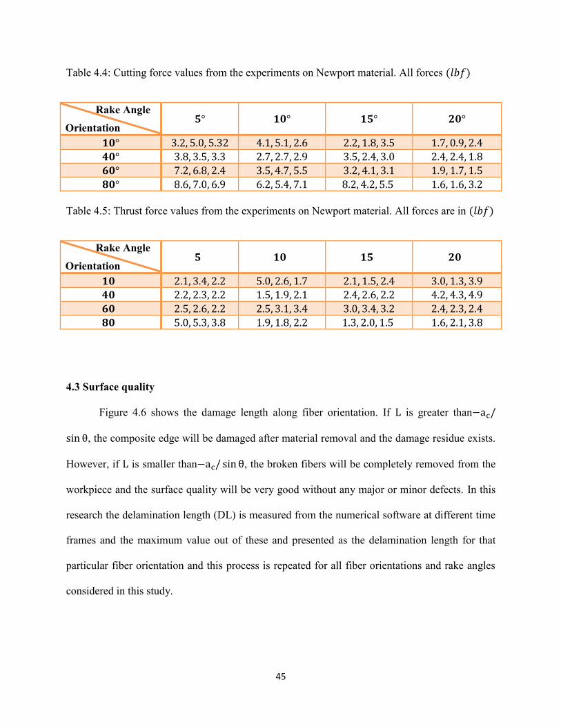
Table 4.4- Cutting force values from the experiments on Newport material 45

Table 4.5- Thrust force values from the experiments on Newport material 45

Table 5.1: CFRP composite material properties 55

Table 6.1: Numerical simulation delamination lengths (µm) 75

1

CHAPTER I

INTRODUCTION

1.1 Composite Material

Composites in general are combination of two or more materials and their technology

dates back few centuries early when straws was first used in clay to form composite brick. As

time evolved their definition was refined and now, it‟s defined as the combination of two or

more materials which differ in their physical and chemical form, where their constituents can be

easily differentiated. The ability to tailor these materials to the specific needs and their superior

properties are the driving force behind this increased utilization. Composite materials have high

strength to weight ratio know as the specific strength as compared to conventional materials,

hence used a lot in aerospace industry.

1.2 Constituent Materials

It has been stated before that composite consist of two or more distinctly different

materials. In most cases, the composite is made of matrix and reinforcement materials that are

mixed in certain proportions depending on the requirement. Each constituent materials have their

own properties which when combined properly will provide desired results, which is the most

important aspect of composite due to its tailor ability. Fibers have great strength and stiffness

which when combined with weaker matrix will result in a composite with lesser properties than

the actual fibers, but the overall composite properties in general will have considerable

difference to that of conventional materials.

2

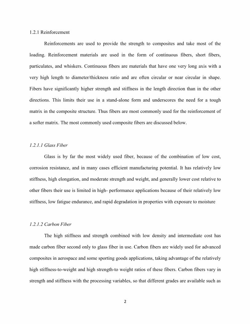
1.2.1 Reinforcement

Reinforcements are used to provide the strength to composites and take most of the

loading. Reinforcement materials are used in the form of continuous fibers, short fibers,

particulates, and whiskers. Continuous fibers are materials that have one very long axis with a

very high length to diameter/thickness ratio and are often circular or near circular in shape.

Fibers have significantly higher strength and stiffness in the length direction than in the other

directions. This limits their use in a stand-alone form and underscores the need for a tough

matrix in the composite structure. Thus fibers are most commonly used for the reinforcement of

a softer matrix. The most commonly used composite fibers are discussed below.

1.2.1.1 Glass Fiber

Glass is by far the most widely used fiber, because of the combination of low cost,

corrosion resistance, and in many cases efficient manufacturing potential. It has relatively low

stiffness, high elongation, and moderate strength and weight, and generally lower cost relative to

other fibers their use is limited in high- performance applications because of their relatively low

stiffness, low fatigue endurance, and rapid degradation in properties with exposure to moisture

1.2.1.2 Carbon Fiber

The high stiffness and strength combined with low density and intermediate cost has

made carbon fiber second only to glass fiber in use. Carbon fibers are widely used for advanced

composites in aerospace and some sporting goods applications, taking advantage of the relatively

high stiffness-to-weight and high strength-to weight ratios of these fibers. Carbon fibers vary in

strength and stiffness with the processing variables, so that different grades are available such as

3

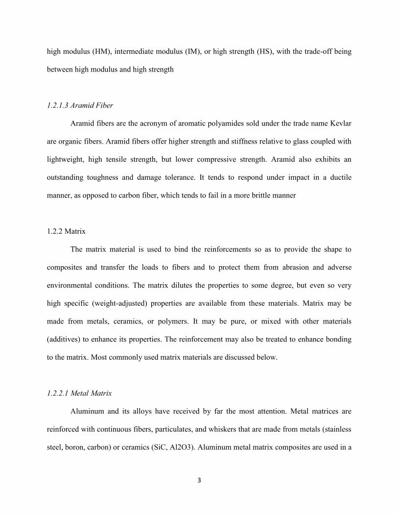
high modulus (HM), intermediate modulus (IM), or high strength (HS), with the trade-off being

between high modulus and high strength

1.2.1.3 Aramid Fiber

Aramid fibers are the acronym of aromatic polyamides sold under the trade name Kevlar

are organic fibers. Aramid fibers offer higher strength and stiffness relative to glass coupled with

lightweight, high tensile strength, but lower compressive strength. Aramid also exhibits an

outstanding toughness and damage tolerance. It tends to respond under impact in a ductile

manner, as opposed to carbon fiber, which tends to fail in a more brittle manner

1.2.2 Matrix

The matrix material is used to bind the reinforcements so as to provide the shape to

composites and transfer the loads to fibers and to protect them from abrasion and adverse

environmental conditions. The matrix dilutes the properties to some degree, but even so very

high specific (weight-adjusted) properties are available from these materials. Matrix may be

made from metals, ceramics, or polymers. It may be pure, or mixed with other materials

(additives) to enhance its properties. The reinforcement may also be treated to enhance bonding

to the matrix. Most commonly used matrix materials are discussed below.

1.2.2.1 Metal Matrix

Aluminum and its alloys have received by far the most attention. Metal matrices are

reinforced with continuous fibers, particulates, and whiskers that are made from metals (stainless

steel, boron, carbon) or ceramics (SiC, Al2O3). Aluminum metal matrix composites are used in a

4

vast number of applications where strength and stiffness are required. This includes structural

members in aerospace applications and automotive engine components

1.2.2.2 Ceramic Matrix

Ceramic matrix composites mostly use ceramics for both the matrix phase and the

reinforcement phase. Because of the excellent thermal stability and high stiffness of ceramics,

their composites are attractive for applications where high strength and high stiffness are

required at high temperatures.

1.2.2.3 Polymer Matrix

Polymer matrices by far are most widely used in composites applications. The wide range

of properties that result from their different molecular configureurations, their low price and ease

of processing make the perfect material for binding and enclosing reinforcement. Polymer

matrices are normally reinforced with glass, carbon, and aramid fibers. Polymer matrix

composites have found a wide range of applications in sports, domestic, transportation, and

aerospace industries

Composites are broadly classified according to the type of matrix material

Metal matrix composites

Ceramic matrix composites

Polymer matrix composites

It is further classified according to the reinforcement form and arrangement

Particulate reinforced (random, preferred orientation)

5

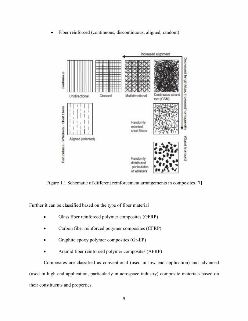
Fiber reinforced (continuous, discontinuous, aligned, random)

Figure 1.1 Schematic of different reinforcement arrangements in composites [7]

Further it can be classified based on the type of fiber material

Glass fiber reinforced polymer composites (GFRP)

Carbon fiber reinforced polymer composites (CFRP)

Graphite epoxy polymer composites (Gr-EP)

Aramid fiber reinforced polymer composites (AFRP)

Composites are classified as conventional (used in low end application) and advanced

(used in high end application, particularly in aerospace industry) composite materials based on

their constituents and properties.

6

Advanced composites are superior in properties and generally use continuous fibers to

achieve the desired properties in required direction, like, high specific strength (most basic

requirement for an aircraft) and stiffness. Continuous fibers are those which have very high

length to diameter ratio and often incorporated into a composite in desired orientation.

Fiber Reinforced Polymers (FRP‟s) are a class of advanced composites which uses fibers

as the reinforcement which provides strength to the composite and polymers as the matrix which

bonds to the fibers, providing shape and transferring load to the fibers.

These materials are characterized by their high specific strength and high specific

stiffness. They are also excellent corrosion resistance materials and provide better resistance to

fatigue loading. This makes them suitable for various applications in the chemical, marine,

transportation, and aerospace industries. In addition, they find wide applications in the sporting

and leisure industries.

1.3 Composite Properties

Properties of composites, particularly continuous-fiber reinforced, are different from

those of metals in that they are highly directional. A material is called anisotropic when its

properties at a point vary with direction. The orientation of the reinforcement within the matrix

affects the state of isotropy of the material

Properties of composites are also described with respect to the scale at which the material

is analyzed. Consider a composite lamina, which is the simplest possible form of a composite

consisting of an assembly of anisotropic fibers in an isotropic matrix. At the microscopic scale,

7

analysis is conducted at the fiber diameter level. This is called micromechanics analysis and it

deals with relationships between stress and deformation in the fibers, matrix and fiber–matrix

interface. Micromechanics analysis allows for the prediction of the average lamina properties as

a function of the properties of the constituents and their relative amounts in the structure. At the

macroscopic level, the lamina is treated as a whole and the material is considered as

homogeneous and anisotropic. Lamina average properties are used to study the overall lamina

behavior under applied loads. Macromechanics is also concerned with analysis of the behavior of

laminates consisting of multiple laminas stacked in a certain sequence based on the average

properties of the lamina.

1.3.1 Density

Consider a composite consisting of matrix and reinforcement phases of known densities.

The weight of the composite, wc is given by the sum of the weights of its constituents, wf and wm

wc = wf+wm, (1.1)

Where, the subscripts f and m refer to the reinforcement and the matrix, respectively.

Substituting for w by ρ v, above can also be written as

ρcvc =ρfvf+ρmvm, (1.2)

Where vc, vf, and vm denote the volume of the composite, reinforcement, and matrix,

respectively. Dividing (1.2) by vc it becomes

ρc =ρfVf+ρmVm, (1.3)

8

Where Vf and Vm denote the volume fractions of the constituents, vf/vc and vm/vc,

respectively. Equation (1.3) is known as the law of mixtures and it shows that the density of a

composite is given by the volume fraction adjusted sum of the densities of the constituents.

1.3.2 Elastic Properties

The composite lamina is assumed to be macroscopically homogeneous and linearly

elastic. The matrix and the fibers are assumed to be linearly elastic and homogeneous, with the

fibers being also anisotropic (transversely isotropic). The interface is completely bonded and

both the fiber and matrix are free of voids. The response of the lamina under load can be

analyzed using a parallel model or a series model. In the parallel model (also called Voigt model

and equal strain model), it is assumed that the fiber and the matrix undergo equal and uniform

strain. This leads to the following expression for stiffness in the longitudinal direction

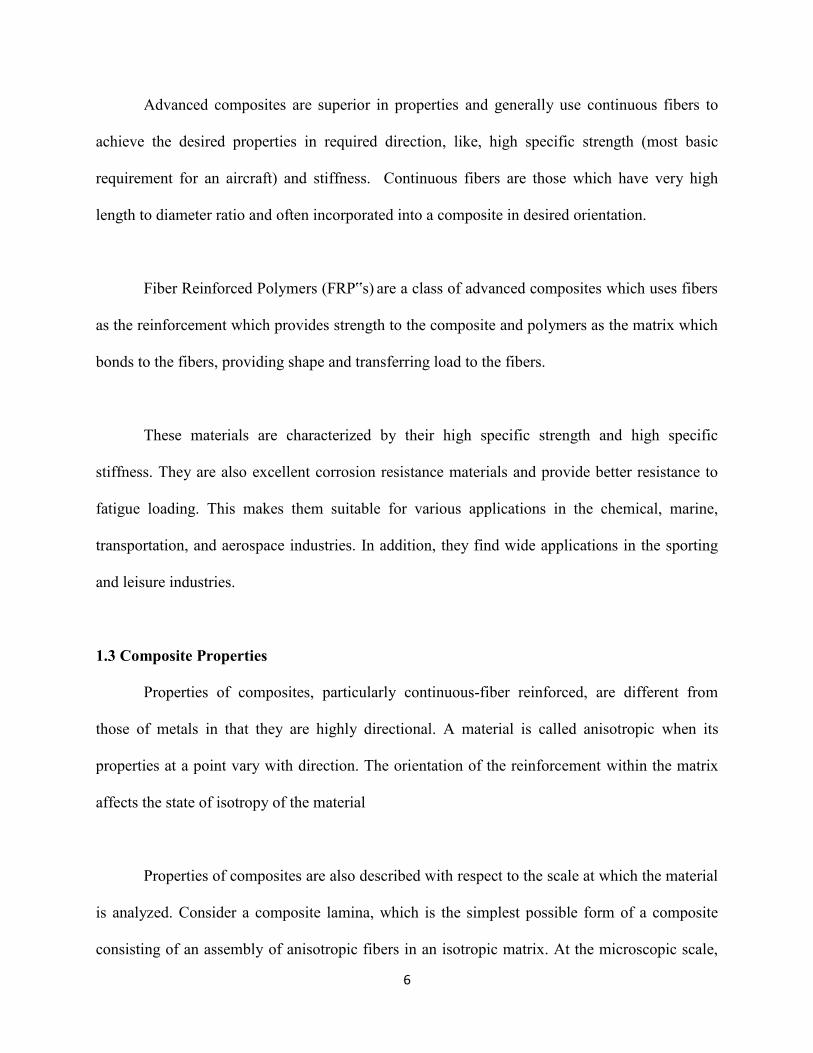
E1 =VfE1f+VmEm. (1.4)

Figure 1.2 Principal material orientation of composite laminate [7]

Here the subscripts 1f refer to the longitudinal direction of the fibers. Note that (1.7) is

similar to (1.3) and it gives the elastic modulus as the weighted mean of the fibers and the matrix

9

modulus. In a series model (also called Ruess model), it is assumed that the fibers and the matrix

are under equal and uniform stress. This leads to the following expression for compliance along

the longitudinal direction

C1 =VfC1f+VmCm. (1.5)

Knowing that C = 1/E, (1.5) is rewritten as

E1 = E1fEm / (VfEm+VmE1f) (1.6)

.

In similar manners, the remaining equations for the major Poisson ratio and in plane

shear modulus are determined using the equations

ν12 =Vfν12f+Vmνm, (1.7)

G12 = G12fGm / (VfGm +VmG12f). (1.8)

1.4 Research Objective

By considering the above it is clear that composites are totally different to that of metals

so does their machinability and also there is little research conducted on composites, hence it will

be useful to investigate the machinability of composites. The objective of this research is to study

both experimentally and numerically the effect of two most important machining parameters,

fiber orientation and rake angle on surface quality in particular delamination/debonding, the

delamination is a series issue affecting the structural integrity and service life. This will lead to

better understanding of machinability of composites, their by leading to better design of

materials, tooling and cutting conditions.

10

CHAPTER II

LITERATURE REVIEW

Everstine and Rogers [8] were the first to submit their theoretical work based on

continuum mechanics approach to predict the minimum cutting force required to machine 0o

fiber orientation. Koplev et al [1] were one of the first to experimentally study the machining

process of FRP‟s, which set the foundation for future research and publications.

According to their findings the chip formation in orthogonal machining was highly

dependent on fiber orientation and consisting of series of fractures each creating a chip, the study

was performed for fibers both parallel and perpendicular to the feed direction. Many have

studied the effect of tool geometry, cutting conditions and material properties on cutting forces,

chip formation, tool wear and surface quality to observe the machining kinematics of

composites.

Takeyama and Iijima [14] developed a model to predict cutting forces independent of

fiber orientation, also concluding the chip formation for most fiber angled composites to be

similar to that of metals. One of the major findings in the literature indicate the in-plane shear

strength for FRP‟s plays an important role while machining, at the same time there were no

universally accepted standard test to come up with the shear strength of FRP‟s. It was later

found that Iosipescu Shear Test can be used with some modification to simulate the orthogonal

machining at very low cutting speeds [15].

11

In general, results from machining of FRP‟s can be obtained either experimentally or

numerically depending on the facilities available. Numerical simulations are usually used to

support the experimental findings and to further apply to obtain new findings where the

experimental investigations become difficult and expensive

2.1 Machining Models

2.1.1 Everstine and Rogers Model

Everstine and Rogers [8] had proposed a theory on machining of FRP composites. The

model predicts the minimum cutting force required for machining parallel unidirectional fibers

based on a continuum mechanics approach [9]. They proposed a displacement field for the chip

region analogous to the thick-zone model in cutting of metals that was proposed by Palmer and

Oxley [10]. They explained the formation of wrinkle ahead of tool tip owing to tensile loading

from the chip separation. Plastic deformations are determined kinematically, the deformation is

found by using suitable displacement boundary condition and constraint conditions [12]. They

proposed an estimate for the principle cutting force, Fc in terms of the tool geometry, material

properties and the proposed deformation. The schematic diagram of their cutting mechanism is

shown in Figure 2.1

12

Figure 2.1: Everstine and Rogers Model for Cutting Composites [8]

2.1.2 Koplev model

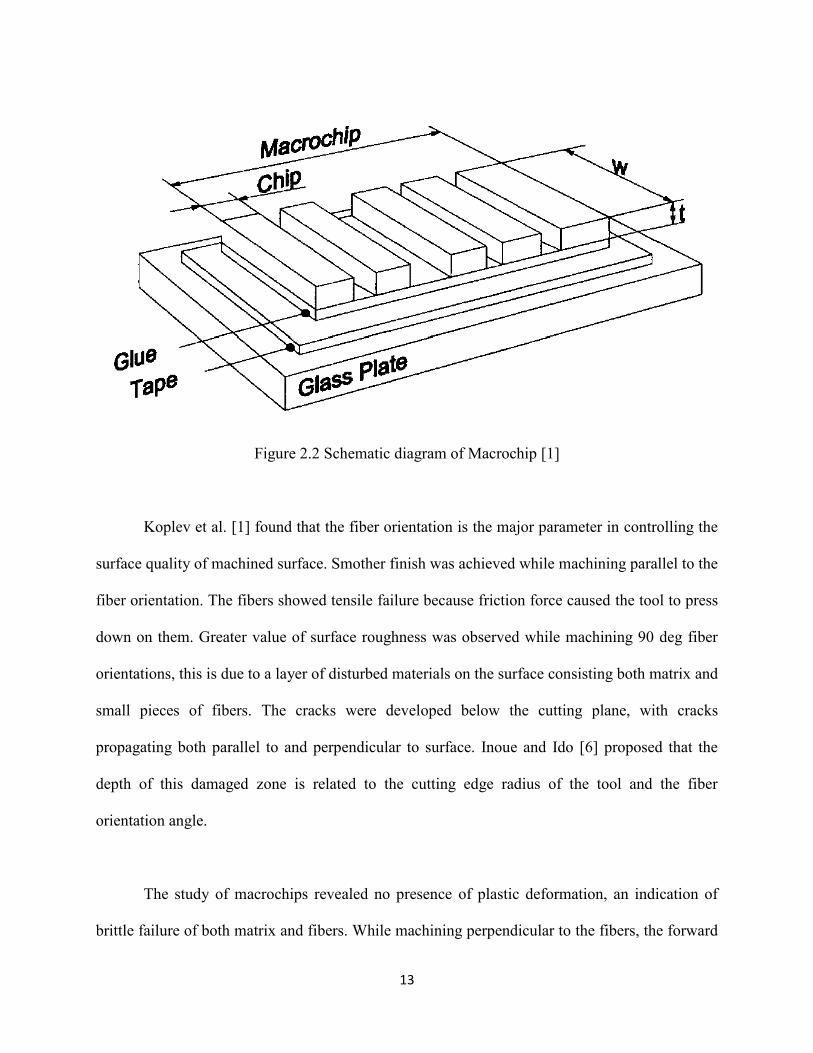
Koplev et al. [1] studied the chip formation process and surface quality of machined

surface while machining the unidirectional CFRP material with a single edged tool. The tests

were carried out for 0 and 90 deg fiber orientation. The chip formation process was investigated

with a quick stop device. The advantage of this study was to make use of macrochip method to

study many small chips produced during machining process. In this method, the workpiece

surface is coated with a thin layer of rubber-based adhesive. After machining, the chips remain

stick to the adhesive. The chips on the adhesive are then examined [13]. A schematic diagram of

macrochip method is shown in following figure

13

Figure 2.2 Schematic diagram of Macrochip [1]

Koplev et al. [1] found that the fiber orientation is the major parameter in controlling the

surface quality of machined surface. Smother finish was achieved while machining parallel to the

fiber orientation. The fibers showed tensile failure because friction force caused the tool to press

down on them. Greater value of surface roughness was observed while machining 90 deg fiber

orientations, this is due to a layer of disturbed materials on the surface consisting both matrix and

small pieces of fibers. The cracks were developed below the cutting plane, with cracks

propagating both parallel to and perpendicular to surface. Inoue and Ido [6] proposed that the

depth of this damaged zone is related to the cutting edge radius of the tool and the fiber

orientation angle.

The study of macrochips revealed no presence of plastic deformation, an indication of

brittle failure of both matrix and fibers. While machining perpendicular to the fibers, the forward

14

movement of the chip presses the composite in front of it, causing the composite to bend and

fracture to form chips. At the same time, the cracks are formed due to the downward pressure on

the composite below the tool. While machining parallel to the fibers, the pressure on the

specimen causes formation of chips. A crack appears in front of tool leading to the start of next

chip. The two machining mechanisms are shown in figure below

Figure 2.3: Chip formations at 900 and 00 fiber orientation [1]

2.1.3 Takeyama and Iijima

Takeyama and Iijima [14] predicted cutting force model by using Merchant‟s minimum

energy theory. They studied the chip formation process when cutting continuous fiber reinforced

plastics at various fiber orientations. Figure 2.4 shows the schematic diagram of orthogonal

cutting process for finer reinforced composite material.

15

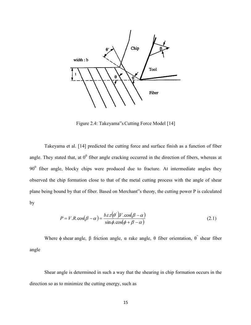
Figure 2.4: Takeyama‟s Cutting Force Model [14]

Takeyama et al. [14] predicted the cutting force and surface finish as a function of fiber

angle. They stated that, at 00 fiber angle cracking occurred in the direction of fibers, whereas at

900 fiber angle, blocky chips were produced due to fracture. At intermediate angles they

observed the chip formation close to that of the metal cutting process with the angle of shear

plane being bound by that of fiber. Based on Merchant‟s theory, the cutting power P is calculated

by

cos.sincos....cos..

' VtbRVP (2.1)

Where ϕ shear angle, β friction angle, α rake angle, θ fiber orientation, θ‟ shear fiber

angle

Shear angle is determined in such a way that the shearing in chip formation occurs in the

direction so as to minimize the cutting energy, such as

16

0)2coscossin '

'

P (2.2)

Where ' experimental model for simple shear test.

Based on the Merchant‟s minimum energy theory and experimental results of ' , the

principal and thrust cutting forces are determined as

sincoscos'

btFp (2.3)

sincossin'

btFt (2.4)

Although the cutting forces predicted from this method are similar to those determined

experimentally. The model failed to explain the phenomenon of the chip formation when

reversing the machining direction, i.e. the model is not valid for materials with fiber orientations

greater than 900. The model also lacked the detailed description of shear test procedure to find

the shear phenomenon and shear strength. For FRP materials, there are no standard techniques to

measure the shear plane angle. Since the chips are generally very small and mostly in the powder

form, it is extremely difficult to measure the chip thickness and so to calculate shear plane angle

as in case of metals. Even the model failed to explain the phenomenon of mean angle of friction

between tool and chip for all the fiber angles.

17

2.1.4 Bhatnagar et al. model

Bhatnagar et al. [2] studied the orthogonal cutting process of unidirectional carbon fiber

composites for different fiber orientations. From their experimental studies, they concluded that

shear strength of the material is an important factor while machining composites. They overcome

the drawbacks of the previous Takayama and Iijima [14] models by proposing a method to

obtain accurate values for the shear strength of composites. Since there was no standard method

to determine the shear strength of the material for any given fiber orientation, they used

Iosipescu shear test method to evaluate the shear strength of material accurately. Based on this

method, they were able to plot the variation of in-plane shear strength with fiber angle.

On machining negative fiber orientation, they found the chip formation to be similar to

that of Koplev et al. The fibers were bent and the chips were formed by delamination of material.

For positive fiber orientation, they found a blocky chip formed by fracture. On further

examinations they found the existence of a plane along which the macrocrack propagated leading

to the formation of chips. This plane also corresponds to that found during Iosipescu shear test.

For machining positive fiber orientations, they concluded that

1. Fibers break in tension to produce the machined surface.

2. Chips are produced ahead of the cutting edge of the tool by shearing of the matrix in a

plane along the fiber orientation.

From the experimental results it was found that the cutting forces were higher for fiber

orientations less than 900. The forces were maximum for fiber orientations between 30 and 600

and minimum between 120 and 1500.

18

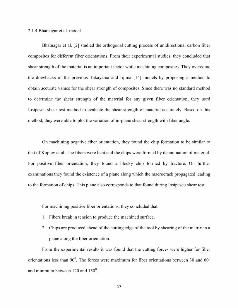
In their model, they were able to predict the effect of fiber orientation on cutting forces

by resolving these forces parallel and perpendicular to the fibers. They schematically showed the

fracture of the fibers separately for negative and positive fiber orientation. This is shown in

figure 2.4.

Figure 2.4: Cutting mechanism of CFRP from Bhatnagar et al. [2]

For negative fiber orientation materials, the progress of the tool causes the fiber to

experience compression and bending. The fibers are pushed upward by the tool and are broken

by shearing. For positive fiber orientation materials, the fibers tend to tilt by the cutting force and

are subjected to tension and bending as well as compression by the tool rake face. They also

observed affects of tensile to shear strength ratio of fibers on the cutting force.

For positive fiber orientation materials, they modeled the cutting process similar to that

proposed by Takeyama and Iijima [14]. They assumed the chip formation along a shear plane

and applied the minimum energy principle. The further assumptions they made are as follows

1. Existence of crack propagation plane along the fiber direction at which matrix shears.

2. The cutting force is dependent on the in-plane shear strength of the fiber angle.

3. The cutting is orthogonal and the fiber angles are in between 0 and 900.

19

4. The coefficient of friction between the tool and chip interface is assumed to vary for each

fiber orientation and the effect of temperature is neglected.

5. Chip formation takes place in a manner to minimize the cutting energy.

6. The matrix shear plane angle is independent of the tool rake angle.

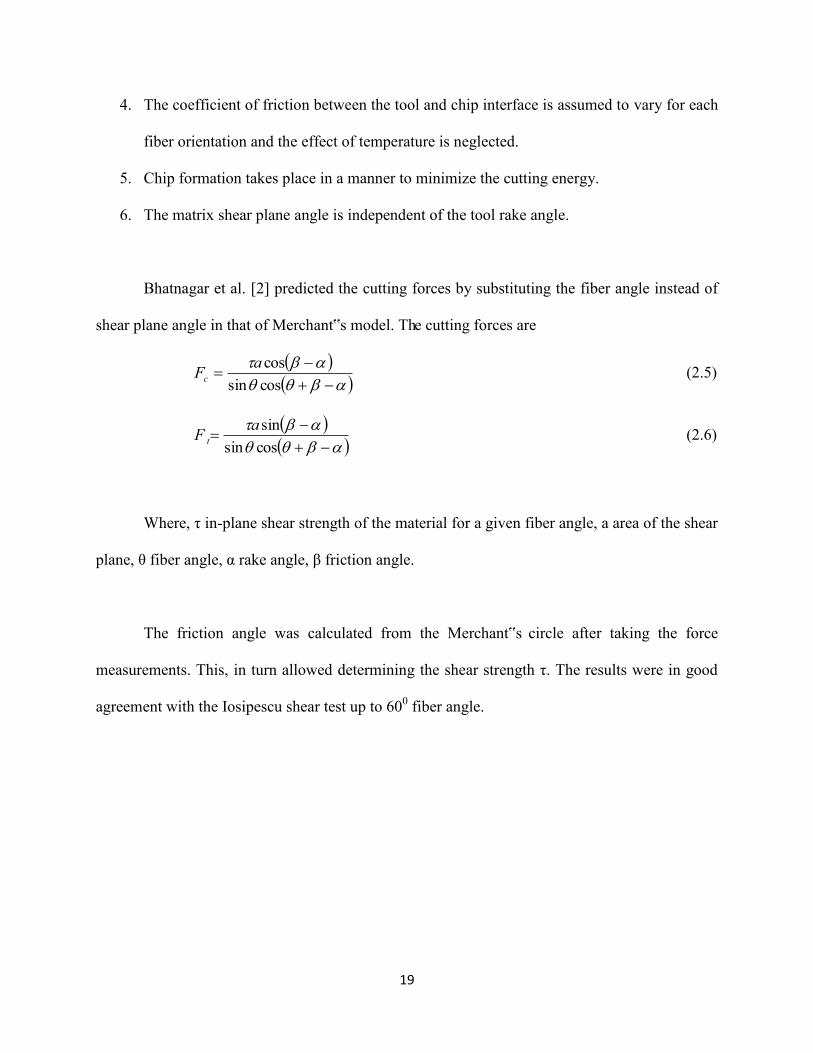
Bhatnagar et al. [2] predicted the cutting forces by substituting the fiber angle instead of

shear plane angle in that of Merchant‟s model. The cutting forces are

cossincosaFc (2.5)

cossinsinaF t (2.6)

Where, τ in-plane shear strength of the material for a given fiber angle, a area of the shear

plane, θ fiber angle, α rake angle, β friction angle.

The friction angle was calculated from the Merchant‟s circle after taking the force

measurements. This, in turn allowed determining the shear strength τ. The results were in good

agreement with the Iosipescu shear test up to 600 fiber angle.

20

CHAPTER III

MACHINING

Machining is a material removal process to remove unwanted material from the work

piece to meet dimensional tolerance and surface finish for further assembly operations.

Machining FRP‟s are different to that of metals because of its inhomogeneous and

anisotropic nature due to the presence of different constituent phases. As the fibers which are

mostly strong and brittle that may have poor thermal conductivity as seen in kevlar fibers,

contrarily, the matrix is weak and ductile. Hence, machining of FRP‟s is characterized by

uncontrolled fracture which is not seen in case metal machining. Also, the machining forces will

be oscillating due to the subsequent cutting of constituents and its machinability is determined by

their physical and mechanical properties. It is also observed to have excessive tool wear while

machining FRP‟s along with fiber pullout and debonding/delamination. This paper will analyze

the cutting forces and surface quality while machining uni-directional FRP‟s.

Machining of metals has been taking place for a very long time and there is extensive

literature on that. Even though, composite materials are totally different to that of metals but

their kinematics remains the same and have been used with proper modifications to cutting tool

geometry, cutting speed and feed rate.

Machining is broadly classified as conventional and non-conventional based on the

machining kinematics.

21

3.1 Conventional Machining

3.1.1 Turning

Turning is used to make cylindrical objects using a single point cutting tool. The

workpiece is rotated through its axis while the cutting tool is fed parallel to its axis of rotation.

As the cutting tool engages with the workpiece, a new surface of revolution is produced by

removing a layer of material whose thickness is equal to the depth of cut. A typical machine tool

for this kind of operation is an engine lathe.

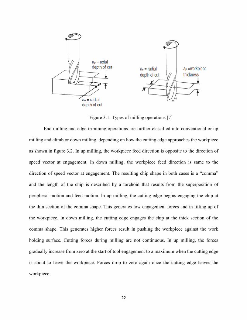
3.1.2 Milling and Trimming

In milling, the rotating cutter that may have one or more cutting edges removes the

material from the workpiece. Most common types of machining FRPs are peripheral milling or

profiling and end milling. Peripheral milling has the cutting edges on the periphery of the tool.

The machined surface is parallel to the cutter axis rotation and the engagement into the

workpiece is in the radial direction as shown in figure 3.1. Peripheral milling is more

appropriately called edge trimming because of smaller diameter tools and the axial engagement

encompasses the entire thickness of the workpiece. End milling is similar to peripheral milling,

except that the axial engagement will be less than the actual thickness of the part and a slot will

be produced.

22

Figure 3.1: Types of milling operations [7]

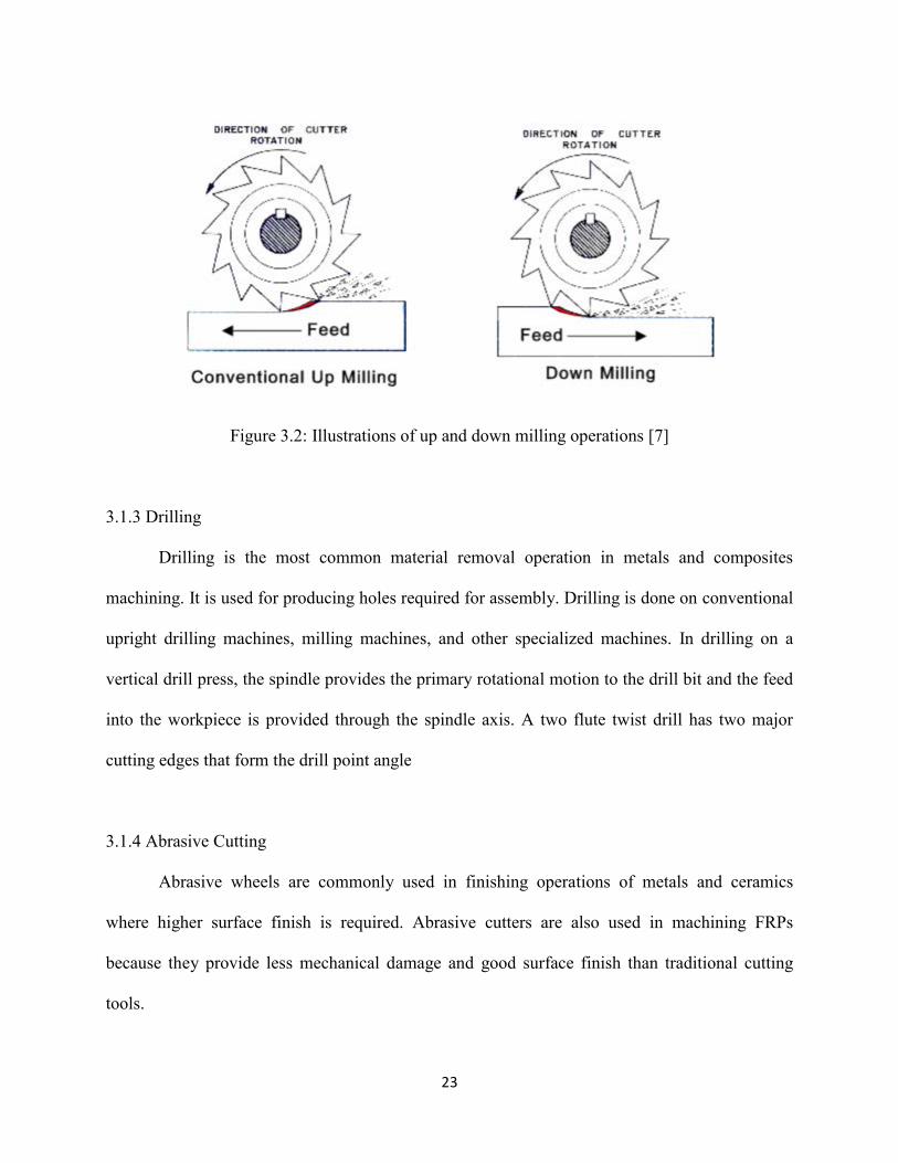
End milling and edge trimming operations are further classified into conventional or up

milling and climb or down milling, depending on how the cutting edge approaches the workpiece

as shown in figure 3.2. In up milling, the workpiece feed direction is opposite to the direction of

speed vector at engagement. In down milling, the workpiece feed direction is same to the

direction of speed vector at engagement. The resulting chip shape in both cases is a “comma”

and the length of the chip is described by a torchoid that results from the superposition of

peripheral motion and feed motion. In up milling, the cutting edge begins engaging the chip at

the thin section of the comma shape. This generates low engagement forces and in lifting up of

the workpiece. In down milling, the cutting edge engages the chip at the thick section of the

comma shape. This generates higher forces result in pushing the workpiece against the work

holding surface. Cutting forces during milling are not continuous. In up milling, the forces

gradually increase from zero at the start of tool engagement to a maximum when the cutting edge

is about to leave the workpiece. Forces drop to zero again once the cutting edge leaves the

workpiece.

23

Figure 3.2: Illustrations of up and down milling operations [7]

3.1.3 Drilling

Drilling is the most common material removal operation in metals and composites

machining. It is used for producing holes required for assembly. Drilling is done on conventional

upright drilling machines, milling machines, and other specialized machines. In drilling on a

vertical drill press, the spindle provides the primary rotational motion to the drill bit and the feed

into the workpiece is provided through the spindle axis. A two flute twist drill has two major

cutting edges that form the drill point angle

3.1.4 Abrasive Cutting

Abrasive wheels are commonly used in finishing operations of metals and ceramics

where higher surface finish is required. Abrasive cutters are also used in machining FRPs

because they provide less mechanical damage and good surface finish than traditional cutting

tools.

24

In abrasive cutters, many diamond particles are brazed or bonded to the tool shank or

body and act as multiple cutting points. Abrasive cutters are mainly classified by the size of the

abrasive particle and the method by which the particles are bonded to the tool body. The size of

abrasive particles is identified by grit number, which is a function of sieve size. The greater the

sieve size, the smaller the grit number.

3.2 Non Conventional Machining

As the demand on high performance composites increases, stronger, stiffer, and harder

reinforcement materials are introduced into modern advanced composite structures. This makes

the secondary machining of these materials increasingly difficult. Traditional machining of

composites is difficult because of its heterogeneity, anisotropy, low thermal conductivity, heat

sensitivity, and high abrasiveness. The stacked nature of most fiber-reinforced composites makes

them also susceptible to debonding between the individual plies as well as within the same ply,

under such conditions it might be efficient using nontraditional machining process.

Nontraditional machining processes include waterjet (WJ), abrasive waterjet (AWJ),

abrasive suspension jet (ASJ), laser and laser-assisted machining, ultrasonic machining, and

electrical discharge machining (EDM). Among this wide range of processes, only AWJ, laser,

and EDM of FRP composites have received considerable attention in the Literature

3.2.1 Abrasive Water Jet machining

High-velocity waterjets have been used since the early 1970s in cutting a variety of

materials, including corrugated board, paper, cloth, foam, rubber, wood, and granite. Abrasive

25

waterjets expand the capabilities of high-velocity waterjets by introducing abrasive particles as

the cutting medium

Currently AWJs are used to cut a wide range of engineering materials including ceramics,

metal alloys, and composites. There are many distinct advantages of AWJ cutting which makes it

desirable over other traditional and nontraditional machining processes. AWJ can virtually cut

any material without any significant heat damage or distortion. Because the cutting forces are

very small and no cutting tools are required, the setup time is shorter than traditional machining

processes and fixturing requirements are either very minimal or not required at all

3.2.2 Laser Machining

Laser machining of FRP composites offers many advantages over traditional machining

processes. There is no contact between the tool and the workpiece, and hence there are no cutting

forces, no tool wear, and no part distortion because of mechanical loading. Laser cutting is a

thermal process and is not influenced by the strength and the hardness of the work material.

Therefore it is best suited for cutting heterogeneous materials composed of different phases with

contrasting mechanical properties. It provides high machining rates, thin kerf width, and

flexibility to cut complex contoured shapes

Drawbacks of laser cutting include material changes and strength reduction due to the

formation of a HAZ, the formation of kerf taper and a decrease in cutting efficiency as thickness

of workpiece increases

26

Even though nontraditional machining have their own advantages and disadvantages but

their use is determined by the final outcome of the process, for e.g., if the process requires higher

production rate then Non-Traditional process (e.g. AWJ) is shown that cutting speeds as high as

2,400 m/min may be used to cut effectively CFRP and GFRP thin parts (6mm thick). This

represents tremendous productivity gains over traditional trimming methods.

If the process requires good surface quality then traditional machining process is used,

the dimensional tolerances and surface finishes also depend on thickness and cutting speed. The

tolerance range that can be held on small parts is about ±0.025mm and on large parts is about

±0.125mm. Tighter tolerances are possible with tighter control of the machine axes and nozzle

motion. Nevertheless, these tolerances do not compare with the tolerance ranges of traditional

machining processes (e.g. ±0.002mm for rough milling and ±0.001mm for finishing).

3.3 Orthogonal Machining

In particular, orthogonal machining is defined as the material removal process in which

the cutting edge is perpendicular to the feed direction and assumed as a 2-dimensional process as

the deformation is mostly confined to a single plane. The surface generated is a plane parallel to

the original work surface. A carpenter‟s plane cuts orthogonally, as does a band saw. Rotary

peeling of veneer approximates orthogonal cutting

It was found that tool material and rake angle have significant effect on the process

output. Figure 3.3 (a) different forces acting during orthogonal machining developed by

Merchant known as Merchant‟s theory of metal cutting. Figure 3.3 (b) shows the schematic of

orthogonal cutting of uni-directional FRP‟s, fiber orientation angle is measured clockwise

27

between feed direction and fiber axis, rake angle is measured between the vertical line and rake

face facilitating the chip flow, clearance angle is measured between the clearance face and the

machined surface which contribute to the thrust force measured perpendicular to the cutting

direction. The intersection of the rake face and the clearance face constitute the cutting edge

responsible for the cutting force measured along the cutting direction.

Figure 3.3: Schematic of orthogonal cutting (a) Metals (b) UD-FRP (0 < θ < 90) [2]

3.4 Chip Formation Modes

The process of chip formation in orthogonal machining of unidirectional fiber reinforced

composites was studied by several researchers. Koplev et al. [8] were among the first to study

this phenomena using the quick stop device and macro chip methods. The quick stop device is

widely used in the study of metal machining, and is well documented in the metal cutting

literature [2] and thus will not be discussed here

The chip formation process in machining unidirectional FRPs is categorized into five

different types, depending on fiber orientation and cutting edge rake angle. Figure 3.4

schematically shows the different modes of chip formation when machining FRPs with a sharp

cutting edge (nose radius in the order of a few micrometers) and the resulting chip types.

28

Delamination type chip formation (Type I) occurs for the 0◦ fiber orientation and positive rake

angles as shown in figure. 3.4 (a). Mode I fracture and loading occur as the tool advances into

the work material. A crack initiates at the tool point and propagates along the fiber–matrix

interface. As the tool advances into the workpiece, the peeled layer slides up the rake face,

causing it to bend like a cantilever beam. Bending-induced fracture occurs ahead of the cutting

edge and perpendicular to the fiber direction. A small distinct chip segment is thus formed and

the process repeats itself again. The fractured chip flattens out upon separation and returns to its

original shape because of the absence of plastic deformation. The cutting forces widely fluctuate

with the repeated cycles of delamination, bending, and fracture. The machined surface

microstructure reveals fibers partly impeded in the epoxy resin matrix because of elastic

recovery and the fracture patterns of the matrix suggest that it was stretched in Mode I loading

before fracture. Fibers on the machined surface are fractured perpendicular to their direction as a

result of micro buckling and compression of the cutting edge against the surface. Figure 3.4 (a)

shows an example of the machined surface for delamination type chip formation [14].

Fiber buckling type of chip (Type II) occurs when machining 0◦ fiber orientation with 0◦

or negative rake angles as shown in figure. 3.4 (b). In this case, the fibers are subjected to

compressive loading along their direction, which causes them to buckle. Continuous

advancement of the cutting tool causes Mode II loading (sliding) or in-plane shearing and

fracture at the fiber–matrix interface. Successive buckling finally causes the fibers to fracture in

a direction perpendicular to their length. This fracture occurs in the immediate vicinity of the

cutting edge and results in small discontinuous chips.

29

The cutting forces fluctuation in this case is smaller than that for the delamination type

(Type I) chip formation process. The machined surface for the buckling type chip is also similar

to that of the delamination type chip machined surface. Fiber cutting type chip formation occurs

when machining fiber orientations greater than 0deg and less than 90deg, and for all rake angles

as shown in figure. 3.4 (c–e). The chip formation mechanism consists of fracture from

compression-induced shear across the fiber axes followed by interlaminar shear fracture along

the fiber–matrix interface during the cutting tool advancement. During the compression stage of

the chip formation process, cracks are generated in the fibers above and below the cutting plane.

The cracks below the cutting plane remain in the machined surface and are visible when

examined under microscope. Chip flow in machining all positive fiber angles up to 90◦ thus

occurs on a plane parallel to fiber orientation. This makes this particular type of chip formation

similar in appearance to the chip formation in metal cutting where material is deformed by

plastic shear as it passes across a shear plane. An important distinction, however, is the absence

of plastic deformation in the case of machining FRPs. Material removal in these cases appears to

be governed by the in-plane shear properties of the unidirectional composite material

30

Figure 3.4: Cutting mechanisms in orthogonal machining CFRP with sharp edges [4]

3.5 Machining Tools

Machining of fiber-reinforced polymers (FRPs) is a challenging process from the point of

cutting tool requirements. Unlike metal cutting where plastic deformation is the predominant

cause of chip formation, the cutting of FRPs takes place by compression shearing and fracture of

the fiber reinforcement and matrix. This puts stringent requirements on the cutting edge

geometry and material. A sharp cutting edge and large positive rake angle are often required to

facilitate clean shaving of the fibers, and a tool material with high hardness and toughness is

31

required to resist the abrasiveness of the fibers and the intermittent loads generated by their

fracture

A wide range of cutting tool materials is available for machining applications. These

materials are generally classified into three main groups according to their hardness, strength,

and toughness, as shown in figure. 3.5, which also demonstrates the opposing relationship

between hardness and toughness. The three groups are high-speed steels (HSS), cemented

carbides, and ceramics/super hard materials. Each group has its own characteristic mechanical

and thermal properties, which makes its application more suitable for certain machining

operations

Figure 3.5: Interrelations between toughness and hardness for the tool materials [7]

32

3.6 Tool Geometry

A cutting tool has one or more sharp cutting edges. The cutting edges separate the chips

from the workpiece. A cutting tool is selected to suit a particular machining operation.

Rake face directs the flow of the newly formed chip, is oriented at a certain angle called

the rake angle. Range mostly +50 to -50; some +100 to -100; a few +200 to -200.

Flank face, which provides a clearance between the tool and the newly generated work

surface, and is oriented at an angle called the clearance angle and ranges positive 20-100

Chip Breakers are frequently used with single-point tools to force the chips to curl more

tightly than they would naturally be inclined to do, thus causing them to fracture.

A single-point tool has a main cutting edge and a tool point from which the name of this

cutting tool is derived.

A Multiple edge cutting tool has more than one cutting edge and usually achieves their

motion relative to the work part by rotating.

3.7 Tool Wear

Tool wear is defined as the unwanted removal of tool material from the cutting edge or

the permanent deformation of the cutting edge leading to undesirable changes in the cutting edge

geometry. Once the initial cutting geometry is altered, the cutting tool becomes less effective in

performing its principal functions, which are material removal and generating good quality

machined surface. Tool wear leads to undesirable consequences such as reduction in cutting edge

33

strength, increased tool forces and power consumption, increased cutting temperatures,

degradation in surface finish, loss of part dimensional accuracy, and eventually loss of

productivity. Therefore, it is extremely desirable that tool wear is considerably minimized and

controlled.

3.7.1 Types of Tool Wear

Flank wear in which the portion of the cutting tool at contact with the finished part is

worn out and can be used in tool life expectancy equation.

Crater wear is on the rake face as the flowing chips erodes away some of the face. This

type of tool wear is common, and does not seriously affect the use of a tool until it

becomes larger enough to cause a cutting edge failure.

It can be caused by very low spindle speed or very high feed rate. In orthogonal machining this

typically occurs where the tool temperature is highest.

Built-up edge in which workpiece material sticks on to the cutting edge. Some materials

(copper and aluminum) have the tendency to anneal themselves to the cutting tool edges.

It occurs frequently while machining softer metals that has low melting point. It can be

prevented by good lubrication and increasing cutting speeds.

Edge wear refers to wear on the outer edges of a drill bit around the cutting face caused

due to excess cutting speed.

34

3.8 Tool life

Tool life is defined as the cutting time required for reaching an amount of wear as

specified by a tool-life criterion. A tool-life criterion is defined by a machining objective such as

predetermined acceptable levels of cutting forces, surface quality, dimensional stability, or

production rate

3.9 Machining Forces

In orthogonal cutting, the tool edge is perpendicular to the direction of the cutting speed

vector, v. Orthogonal cutting represents a two-dimensional problem, and hence, it lends itself

well to research work. In orthogonal cutting, all forces, motions, and deformations are in the

plane formed by the cutting velocity vector and the direction normal to the following

assumptions are made to further simplify the analysis

The tool cutting edge is perfectly sharp and straight, cuts perpendicular to the

direction of motion, and has a width greater than that of the workpiece.

The cutting edge generates a plane surface, at constant depth of cut as the work

moves past it with a uniform velocity.

The chip does not flow to either side, since it has the same width as the workpiece.

A continuous chip is produced without a built-up edge.

The shear surface is a plane extending upward from the cutting edge.

There is no contact between the workpiece and the clearance surface of the tool.

35

Figure 3.6: Force equilibrium on shear plane in orthogonal machining [7]

The cutting ratio r is defined by as ac/ao. The relationship between r and φ can be

obtained from Figure. 3.6 as follows

sinφ = ac / AB

r = ac / ao

= AB sinφ / (AB cos(φ −αo))

= sinφ / cos(φ −αo) (3.1)

tanφ = r cosαo / (1−r sinαo) (3.2)

The force Ff represents the frictional resistance met by the chip as it slides over the rake

face of the tool, Fn is known as the normal force from figure. 3.6. The ratio of Ff to Fn is the mean

coefficient of friction, μ. Forces on the rake face are

Ff = Fcsinαo +Ftcosαo = R cos(90−β ) (3.3)

Fn = Fccosαo −Ftsinαo = R sin(90−β ) (3.4)

36

μ = tanβ = Ff / Fn

= [Fcsinαo +Ftcosαo] / [Fccosαo –Ftsinαo] (3.5)

The cutting force, Fc, in the direction of the relative motion between the tool and

workpiece determines the amount of work required to remove material. The thrust force, Ft, is

normal to the relative motion between the tool and workpiece and does no work. Thus, the

machining power is defined as

Pm = Fcv. (3.6)

The specific cutting energy also called the specific cutting pressure is the machining

power per unit volume removed per unit time

Ps = Fcv / vAc

= Fc / Ac (3.7)

A high degree of fluctuation in the cutting forces is exhibited when machining FRPs. The

fluctuations in the principal or cutting force are observed to be higher than those in the thrust

force. The degree of fluctuation depends primarily on fiber orientation and it correlates to a large

extent with the mode of chip formation prevalent in cutting the particular fiber orientation as

explained in Figure. 3.4. For cutting parallel to the fibers with positive rake angle, the force

fluctuations are indicative of the peeling and bending/fracture action of the fibers occurring on

the rake face. For cutting positive fiber orientations, the principal force reflects changes in the

process of shearing and fracture of the fiber and matrix materials with changes in fiber

orientation. The thrust force reflects the interaction between the machined surface and the

clearance face of the tool

37

3.10 Surface Quality

In any machining operations, a specific surface geometry is produced as a result of the

prescribed machine tool kinematics. This surface geometry is called an ideal or theoretical

surface geometry, which follows a repeated pattern. In real life, however, the actual machined

surface deviates from the ideal surface because of tool wear, machine vibrations, material

inhomogeneity, and other factors not related to machine tool kinematics. The actual machined

surface may not have a regular geometry which is called natural surface finish

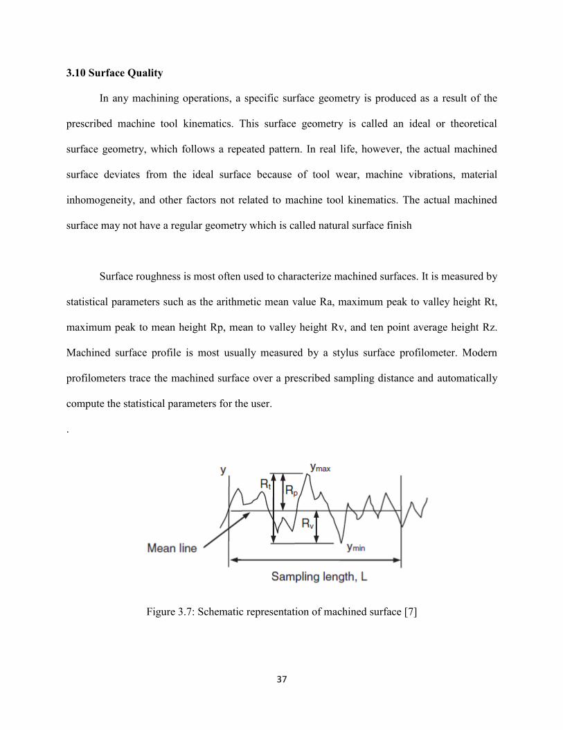
Surface roughness is most often used to characterize machined surfaces. It is measured by

statistical parameters such as the arithmetic mean value Ra, maximum peak to valley height Rt,

maximum peak to mean height Rp, mean to valley height Rv, and ten point average height Rz.

Machined surface profile is most usually measured by a stylus surface profilometer. Modern

profilometers trace the machined surface over a prescribed sampling distance and automatically

compute the statistical parameters for the user.

.

Figure 3.7: Schematic representation of machined surface [7]

38

Machined surface quality is often characterized by surface morphology or texture and

surface integrity. Surface morphology is concerned with the geometrical features of the

generated surface. It is a function of the tool geometry, kinematics of the machining process, and

machine tool rigidity. Surface integrity describes the physical and chemical changes of the

surface layer after machining. This includes fiber pullout, fiber breakage, delamination, matrix

removal, and matrix melting or decomposition. Both surface morphology and integrity depend

on process and workpiece characteristics such as cutting speed, feed rate, fiber type and content,

fiber orientation, and matrix type and content.

The reliability of machined components, especially of high strength applications, is

critically dependent on the quality of the surfaces produced by machining. The condition of the

surface layer of the machined edge may drastically affect the strength and the chemical

resistance of the component. It is necessary, therefore, to characterize and quantify the quality of

the machined surface and the effect of process parameters on surface quality

39

CHAPTER IV

EXPERIMENTAL SETUP AND PROCESS PARAMETERS

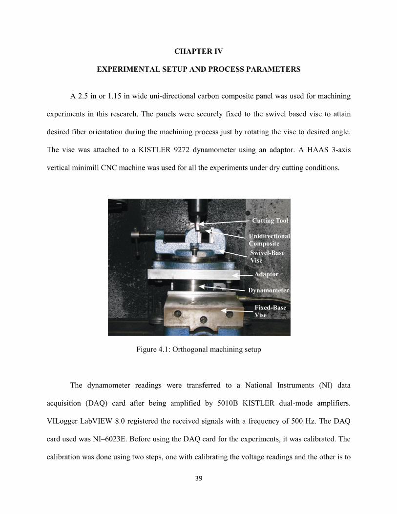
A 2.5 in or 1.15 in wide uni-directional carbon composite panel was used for machining

experiments in this research. The panels were securely fixed to the swivel based vise to attain

desired fiber orientation during the machining process just by rotating the vise to desired angle.

The vise was attached to a KISTLER 9272 dynamometer using an adaptor. A HAAS 3-axis

vertical minimill CNC machine was used for all the experiments under dry cutting conditions.

Figure 4.1: Orthogonal machining setup

The dynamometer readings were transferred to a National Instruments (NI) data

acquisition (DAQ) card after being amplified by 5010B KISTLER dual-mode amplifiers.

VILogger LabVIEW 8.0 registered the received signals with a frequency of 500 Hz. The DAQ

card used was NI–6023E. Before using the DAQ card for the experiments, it was calibrated. The

calibration was done using two steps, one with calibrating the voltage readings and the other is to

40

convert the voltage to the desired physical quantity. The X and Y forces of the dynamometer

which corresponds to the cutting and thrust forces respectively were calibrated with standard

weights and hanging scale, respectively, and the torque was calibrated with a precise torque

wrench. Figure 4.1 shows the setup used for the experiments. The orientation of the cutting and

thrust forces with respect to the dynamometer coordinate system is shown in figure 4.2.

Figure 4.2: Dynamometer to capture cutting forces

4.1 Methodology

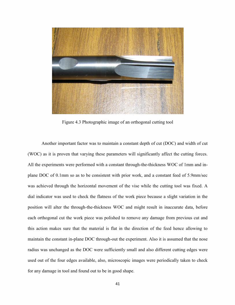
All the experiments were performed using 4-edged orthogonal cutting tool with all four

edges having the same geometry with desired rake and relief angles is shown in figure 4.3. The

tools were attached to the spindle holder which in-turn was attached to spindle head. Since in

orthogonal cutting the cutting edge should be perpendicular to the work piece and should remain

in the position throughout the cutting process the spindle head was rigidly fixed in the desired

position using the spindle orient option or the M19 code. This code provides feedback control for

the spindle in order to keep it stationary. It also reorients the spindle in the same direction any

time the code is run. Hence, maintains the desired rake and relief angles relative to the cutting

direction, the tool should be fit in the tool holder with the correct orientation

41

Figure 4.3 Photographic image of an orthogonal cutting tool

Another important factor was to maintain a constant depth of cut (DOC) and width of cut

(WOC) as it is proven that varying these parameters will significantly affect the cutting forces.

All the experiments were performed with a constant through-the-thickness WOC of 1mm and in-

plane DOC of 0.1mm so as to be consistent with prior work, and a constant feed of 5.9mm/sec

was achieved through the horizontal movement of the vise while the cutting tool was fixed. A

dial indicator was used to check the flatness of the work piece because a slight variation in the

position will alter the through-the-thickness WOC and might result in inaccurate data, before

each orthogonal cut the work piece was polished to remove any damage from previous cut and

this action makes sure that the material is flat in the direction of the feed hence allowing to

maintain the constant in-plane DOC through-out the experiment. Also it is assumed that the nose

radius was unchanged as the DOC were sufficiently small and also different cutting edges were

used out of the four edges available, also, microscopic images were periodically taken to check

for any damage in tool and found out to be in good shape.

42

Figure 4.4: Cutting tool geometry

Figure 4.5: Factors affecting machining forces and surface quality

Machining Forces and Surface Quality(for orthogonal cutting of unidirectional material)

Tool Geometry

Rake Angle

Tool Tip Radius

Material Properties

Fiber OrientationYoung Modulus of FiberFiber Volume Fraction

Fiber DiameterShear Modulus of Fiber

Shear Modulus of MatrixTensile Strength of Fiber

Matrix Shear Strain at Fracture

Machining Condition

Depth of CutFeed Rate

43

Figure 4.4 shows the cutting tool geometry and the measurement of rake and relief angles

used in this study, while figure 4.5 shows the machining parameters that affect the machining

forces and surface quality.

Table 4.1: Orthogonal cutting experiments matrices

Fiber Orientation

Tool Rake Angle

Fiber orientation

Tool Rake Angle

Table 1.1 shows the different fiber orientation and rake angles used in this study while

keeping a constant clearance angle of 6deg and DOC 0.1mm.

4.2 Machining Forces

The experiments were conducted for fiber orientations less than for both Hexplyand Newport

materials. Tables 4.2 to 4.5 show the measured machining forces for both Hexplyand Newport

unidirectional materials. The V I logger system attached to the dynamometer picks up the signal

during machining and stores in an excel format for future viewing and analyzing, figure 4.6

shows one such data of cutting force during machining CFRP, similarly the thrust force will be

acquired for all machining conditions.

44

Figure 4.6: Acquired experimental cutting force for CFRP

Table 4.2: Cutting force values from the experiments on Hexplymaterial. All forces

Rake Angle Orientation

Table 4.3: Thrust force values from the experiments on Hexplymaterial. All forces


-15

-10

-5

0

5

10

15

20

25

30

35

0 0.2 0.4 0.6 0.8 1

Cu

ttin

g Fo

rce

(N

)

Time (S)

Cutting Force

45

Table 4.4: Cutting force values from the experiments on Newport material. All forces


Table 4.5: Thrust force values from the experiments on Newport material. All forces are in


4.3 Surface quality

Figure 4.6 shows the damage length along fiber orientation. If is greater than

, the composite edge will be damaged after material removal and the damage residue exists.

However, if is smaller than , the broken fibers will be completely removed from the

workpiece and the surface quality will be very good without any major or minor defects. In this

research the delamination length (DL) is measured from the numerical software at different time

frames and the maximum value out of these and presented as the delamination length for that

particular fiber orientation and this process is repeated for all fiber orientations and rake angles

considered in this study.

46

Figure 4.7: Delamination (DL) length prediction

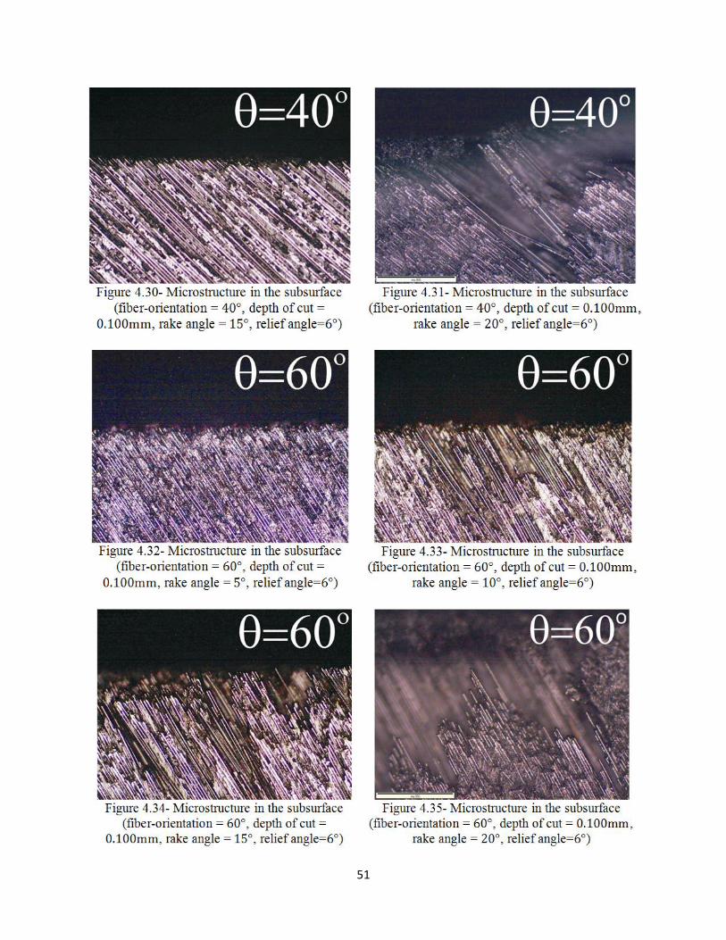
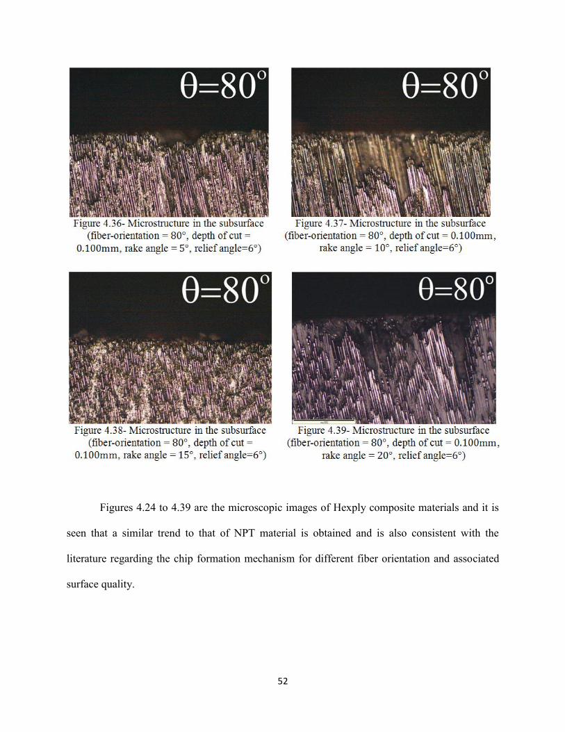
Figures 4.8 to 4.38 shows the microscopic images for fiber orientations 10, 40, 60, and

80deg, rake angles 5, 10, 15, and 20deg for both NPT and Hexply materials, keeping the relief

angle and depth of cut constant at 6deg and 0.100mm respectively. All the images were analyzed

with OLYMPUS compact inverted metallurgical microscope GX 41 which in turn is connected

to soft imaging system for acquisition and processing. The images were taken at three different

locations on the machined surface for each sample and this process was repeated for all the

machined samples. These images were imported to CorelDRAW software were it is been

processed to clearly analyze the machining damage.

49

Figures 4.8 to 4.23 are the microscopic of NPT material and it can be seen that a better

surface quality is obtained for 10 and 40deg fiber orientation and it gets worse for 60 and 80deg

fiber orientation. Also, the effect of rake angles on surface quality is greater for higher fiber

orientation.

52

Figures 4.24 to 4.39 are the microscopic images of Hexply composite materials and it is

seen that a similar trend to that of NPT material is obtained and is also consistent with the

literature regarding the chip formation mechanism for different fiber orientation and associated

surface quality.

53

CHAPTER V

NUMERICAL SIMULATION

Most of the research on machining of composites is experimental, which is tedious and

expensive. However, a good amount of knowledge has been obtained by experimental studies on

the orthogonal machining of unidirectional FRPs which can be used to validate other cheaper and

faster analysis techniques. One such technique is FEA. The use of FEA provides immense

opportunities to study the effect of variables like tool geometry, laminate stacking sequence,

bonding strength between fiber and matrix, operating conditions etc. on cutting forces, chip

formation, surface roughness and the extent of sub-surface damage. An experimental test matrix

to study the effects of the above variables on the cutting forces and chip formation modes would

involve a considerable amount of time and effort.

Simulation of machining of composites is achieved by utilizing the “chip formation

criteria”, which are generally commonly used composite failure criteria such as maximum stress

criterion, Tsai-Hill criterion, Hoffman criterion, etc. These models are developed either by

considering the composite to be an Equivalent Orthotropic Homogeneous Material (EOHM) or

by considering the composite to be a two-phase material consisting of a fiber phase and a matrix

phase. Finite Element Analysis (FEA) of the machining of composites saves a lot of

experimental effort in the determination of machining parameters such as cutting forces, chip

formation mechanism and other workpiece responses to machining. Comparison of experimental

results with those obtained by FEA yields a good correlation between cutting forces and chip

formation modes. The variations of machining parameters with machining conditions are also

discussed for different finite element modeling approaches.

54

The literature available on the FEA of machining of unidirectional FRPs is not very

exhaustive. Arola and Ramulu [18] were the first to simulate the orthogonal cutting of UD-CFRP

composites using finite elements. They considered the work material to be an EOHM and studied

the case where the chip release occurs in the fiber direction. Chip formation was divided into two

stages, (1) primary fracture, involving nodal debonding in front of the tool tip and (2) secondary

fracture, when an appropriate failure criterion (Maximum stress or Tsai-Hill failure criteria in

their study) was satisfied to cause failure at the free-edge. A good correlation was obtained

between the experimental and (FEA) predicted principal cutting force, but large differences were

observed in the thrust force

Nayak et al. were the first to develop a micromechanical approach to model the

workpiece material, which consisted of a fiber phase and a matrix phase. The separation of the

two phases during machining was achieved by using the DEBOND and FRACTURE

CRITERION options in ABAQUS. With such an approach, both the principal and the thrust

force values agreed well with the experimental results. Another side study was the analysis of the

chip formation. In [27], the macro-mechanical approach made it difficult to identify the chip

formation modes

Venu Gopala Rao et al. [15] extended the work of Nayak et al. by including some new

features in their micro-mechanical model, including the isotropic hardening of the matrix,

stiffness degradation of the matrix once the yield stress has been reached, and using cohesive

zone model (CZM) for debonding at the fiber-matrix interface, in which the fracture energies for

Mode I and Mode II fractures are used to simulate debonding

55

In general, the EHM approach gives good estimates of global properties such as cutting

forces but cannot be used to study chip formation mode and geometry. The micro-mechanical

approach provides better accuracy, but both these approaches consider the machining process to

be 2-dimentional which is not the case in actual machining which might be the cause of

variation. Hence in order to overcome these discrepancies and to model a more realistic

simulation a 3-dimentional approach has been used in this study using a special option available

in ABAQUS 6.9-2.

Table 5.1: CFRP composite material properties

Room Temperature Data

B-Basis (US Units)

Mean (US Units)

B-Basis (SI Units)

Mean (SI Units)

Table 5.1 shows the mechanical properties of CFRP at room temperature for 0 and 90 deg

fiber orientation used in both experimental and numerical study which is NCT 321/G150

56

(NASS) Unitape, the panels were prepared at National Institute of Aviation Research (NIAR)

facility.

Most of the material properties listed in table 5.1 are not readily available as individual

properties of each of the constituents and should be calculated from the mechanical properties of

the composite in whole. Fiber volume fraction is one such essential parameter that must be

known ahead or can be found looking through the cross section of the composite under

microscope in order to calculate the mechanical properties of the components. The properties

from table 5.1 can be used to calculate the individual material properties necessary for the study.

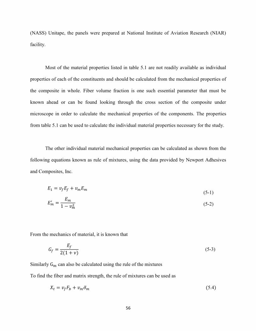
The other individual material mechanical properties can be calculated as shown from the

following equations known as rule of mixtures, using the data provided by Newport Adhesives

and Composites, Inc.

(5-1)

(5-2)

From the mechanics of material, it is known that

(5-3)

Similarly can also be calculated using the rule of the mixtures To find the fiber and matrix strength, the rule of mixtures can be used as

(5.4)

57

The individual fiber strength is much higher than the fiber bundle, especially when the

fiber length is very small. This is because of very few imperfections in fiber that are smaller in

length. In this research, the fiber flexural strength is assumed to be at least times the fiber

bundle strength. The matrix shear strength is estimated to be the same as the composite shear

strength, since it can be assumed that the fiber does not shear.

5.1 Finite Element Modeling

Finite element analysis (FEA) was conducted to measure the fiber-matrix debonding

length. The material was modeled at the microscopic level to better understand the delamination

mechanisms. Fiber and matrix were modeled separately, bonded together using cohesive

elements. Abaqus provides a type of element, which is primarily intended for bonded interfaces

where the bonding properties is defined in the interaction section. The response of these

interactions can be directly expressed in terms of traction versus separation. In the case of

cohesive element and availability of the macroscopic properties of the adhesive material, it may

be more appropriate to model the response using the conventional material model. For the

purpose of this study, the cohesive properties for the interface with the traction-separation

response were used. Cohesive behavior, defined in terms of the traction-separation law is

advisable to predict delamination response.

5.2 Fiber and Matrix Modeling

Fiber was modeled as transversely orthotropic and matrix material was modeled as isotropic with

elastic-plastic behavior and shear damage failure criterion.

58

5.3 Simulation Procedure

Conventionally, in the 2-dimensional machining of homogeneous material, a plane strain

analysis is used, but due to out-of-plane displacements of FRPs during machining, 3D stress

analysis should be used.

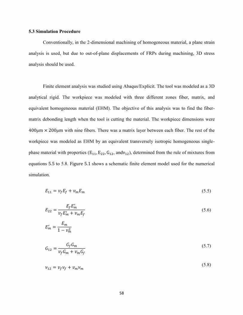
Finite element analysis was studied using Abaqus/Explicit. The tool was modeled as a 3D

analytical rigid. The workpiece was modeled with three different zones fiber, matrix, and

equivalent homogeneous material (EHM). The objective of this analysis was to find the fiber-

matrix debonding length when the tool is cutting the material. The workpiece dimensions were

μ μ with nine fibers. There was a matrix layer between each fiber. The rest of the

workpiece was modeled as EHM by an equivalent transversely isotropic homogeneous single-

phase material with properties ( , and ), determined from the rule of mixtures from

equations 5.5 to 5.8. Figure 5.1 shows a schematic finite element model used for the numerical

simulation.

(5.5)

(5.6)

(5.7)

(5.8)

59

Figure 5.1: Finite element model for 60deg fiber orientation

Carbon fiber was modeled with orthotropic material properties, also EHM zones are not

isotropic, material orientation should be defined for each zone to assign material properties in

their local material orientation. Since orthotropic model is used for carbon fibers and EHM, they

can share the same coordinate system. The bottom of the work piece is constrained in all

directions along with left and right sides; the cutting of composites is done by moving the cutting

tool against the workpiece with the desired velocity. Figure 5.2 shows the exaggerated view of

the cutting zone where the mesh density is very high and gradually decreases away from the zone

to accurately capture the machining response.

60

Figure 5.2: Enlarged view of cutting zone for 60deg fiber orientation

5.4 Element Selection

The Abaqus/Explicit solid element library includes first-order (linear) interpolation

elements and modified second-order interpolation elements in two or three dimensions.

Triangular and quadrilateral first-order elements are available in 2D and tetrahedral, triangular

prism, and hexahedral (brick) first-order elements are available in 3D.

In Abaqus/Explicit you can choose between full or reduced integration for hexahedral

(brick) elements. Only first-order elements with reduced integration are available for

quadrilateral elements in Abaqus/Explicit; the elements with reduced integration are generally

referred to as centroid strain or uniform strain elements with hourglass control. Triangular and

tetrahedral elements are geometrically versatile and are commonly used in many automatic

meshing algorithms. It is convenient to mesh complex shapes with tetrahedral or triangular

61

elements, and the second-order and modified triangular and tetrahedral elements (CPE6,

CPE6M, C3D10, C3D10M, etc.) in Abaqus and is suitable for general purpose applications.

However, a good mesh of hexahedral elements usually provides a solution with better accuracy

at less cost. Quadrilaterals and hexahedra have good convergence rate than triangles and

tetrahedral, and their sensitivity to mesh orientation in regular meshes is not an issue

An 8-node linear brick element with reduced integration and hourglass control is used for

all the simulations with second order accuracy. Distortion control and element deletion option is

used to form chips during and improve convergence because machining involves large

deformations and are sensitive to element deletion.

5.5 Interactions

In Abaqus, there are two ways to define adhesive interaction during simulation either

defining cohesive elements or Surface based cohesive behavior. Cohesive element requires

creating a zone to define traction separation properties. Surface-based cohesive can define the

interaction between two surfaces, these two surfaces are paired and given a cohesive property,

one of them is defined as the master surface and other the slave surface.

Surface-based cohesive behavior and cohesive element are very similar in terms of their

function, but surface-based cohesive behavior is simple to use since it is not necessary to create

additional elements, and can be used in a many applications, such as two sticky surfaces coming

into contact during an analysis. Surface-based cohesive behavior is applicable for situations in

which the interface thickness is negligibly small. If the interface adhesive layer has a finite

thickness and macroscopic properties (such as stiffness and strength) of the adhesive material are

62

to be included, it will be more appropriate to model the response using conventional cohesive

elements.

In this research, there is no separate region for cohesive elements; hence it is more

appropriate to model the work piece using surface-based cohesive behavior because it can

significantly reduce computational cost.

5.6 Analysis Type

The direct-integration dynamic procedure available in Abaqus/Standard offers a choice of

implicit operation for integration of the equations of motion, whereas Abaqus/Explicit uses the

central-difference operation. In implicit dynamic analysis the integration operator matrix must be

inverted and a set of nonlinear equilibrium equations must be solved at each increment of time

step. In an explicit dynamic analysis displacements and velocities are calculated in terms of

quantities that are known at the beginning of an increment step, therefore, the global mass and

stiffness matrices need not be formed and inverted, which means that each increment is

considerably inexpensive compared to that in an implicit integration scheme. The size of the time

increment in an explicit dynamic analysis is limited, however, because the central-difference

operator is only conditionally stable.

Abaqus/Explicit offers fewer element types than compared to Abaqus/Standard. For example,

only first-order, displacement method elements (4-node quadrilaterals, 8-node bricks, etc.) and

modified second-order elements are used, and all degrees of freedom in the model must have

mass or rotary inertia associated with it. However, the method provided in Abaqus/Explicit has

some important advantages as shown below and hence used as the analysis type for all models.

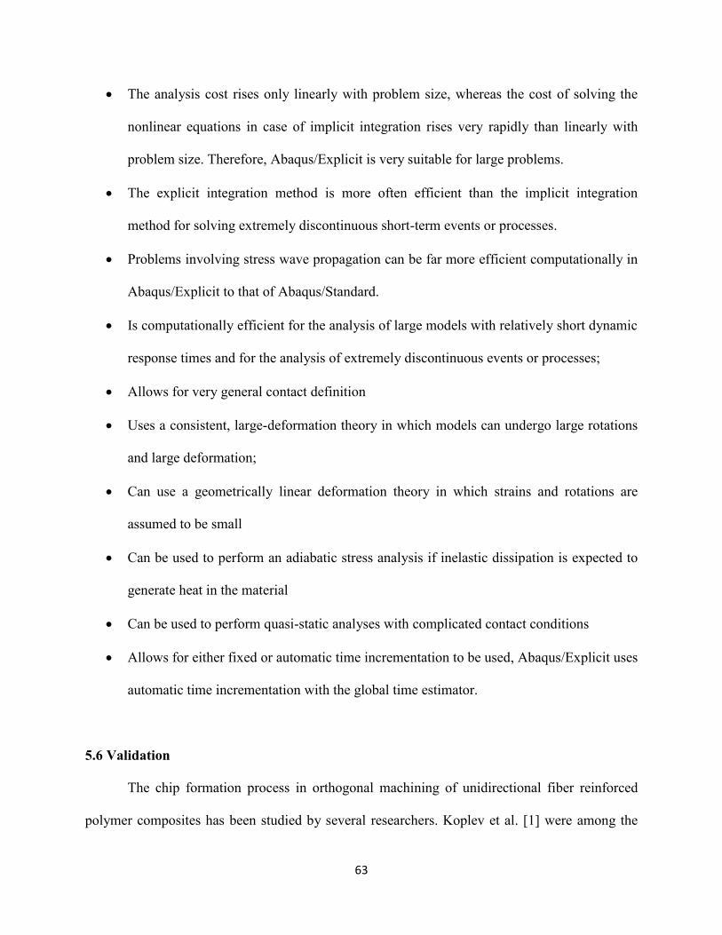
63

The analysis cost rises only linearly with problem size, whereas the cost of solving the

nonlinear equations in case of implicit integration rises very rapidly than linearly with

problem size. Therefore, Abaqus/Explicit is very suitable for large problems.

The explicit integration method is more often efficient than the implicit integration

method for solving extremely discontinuous short-term events or processes.

Problems involving stress wave propagation can be far more efficient computationally in

Abaqus/Explicit to that of Abaqus/Standard.

Is computationally efficient for the analysis of large models with relatively short dynamic

response times and for the analysis of extremely discontinuous events or processes;

Allows for very general contact definition

Uses a consistent, large-deformation theory in which models can undergo large rotations

and large deformation;

Can use a geometrically linear deformation theory in which strains and rotations are

assumed to be small

Can be used to perform an adiabatic stress analysis if inelastic dissipation is expected to

generate heat in the material

Can be used to perform quasi-static analyses with complicated contact conditions

Allows for either fixed or automatic time incrementation to be used, Abaqus/Explicit uses

automatic time incrementation with the global time estimator.

5.6 Validation

The chip formation process in orthogonal machining of unidirectional fiber reinforced

polymer composites has been studied by several researchers. Koplev et al. [1] were among the

64

first to study this phenomena using the quick stop device and macrochip methods. Later, many

researchers have studied this phenomenon using various techniques and finally Wang et al. came

up with the chip formation modes for different fiber orientation and rake angles which is

discussed in detail in chapter II. The numerical simulation obtained for different fiber

orientations with positive rake angle is compared with the literature of Wang et al. and found to

be in good agreement with the modes of chip formation. Although, there are few results available

in literature about the chip formation modes but are mostly experimental findings and could not

predict delamination during machining.

Figure 5.3: Comparison of numerical results with Wang et al. (0 or 180deg fiber orientation)

Figure 5.4: Comparison of numerical results with Wang et al. (45deg fiber orientation)

65

Figure 5.5: Comparison of numerical results with Wang et al. (90deg fiber orientation)

The cutting forces were measured for the experimental machining process as explained in

previous chapter and similarly the cutting forces were measured for the numerical simulation by

activating the contact force between cutting tool and work piece. The numerical cutting forces

were compared with the experimental cutting forces which in turn were compared with literature

and were found to be in good agreement. Fig 5.6 shows the experimental and numerical cutting

force comparison for 20deg rake angle which shows similar trend for different fiber orientations.

For all the experiments three set of readings were taken and shown below and the variations in

the cutting forces is attributed to human errors in maintaining a constant depth and width of cut,

along with the inbuilt variance of the machine, even though after each cut the machined surface

is thoroughly polished their exist some damage in the material which will be inconsistent for

each polish. Also, the material properties are not the same all the way through its length. From

figure 5.6 it can seen that the cutting forces gradually increases as the fiber orientation increases

as observed in the literature due to change in chip formation modes as shown in figures 5.3 to 5.5

and explained in previous chapter.

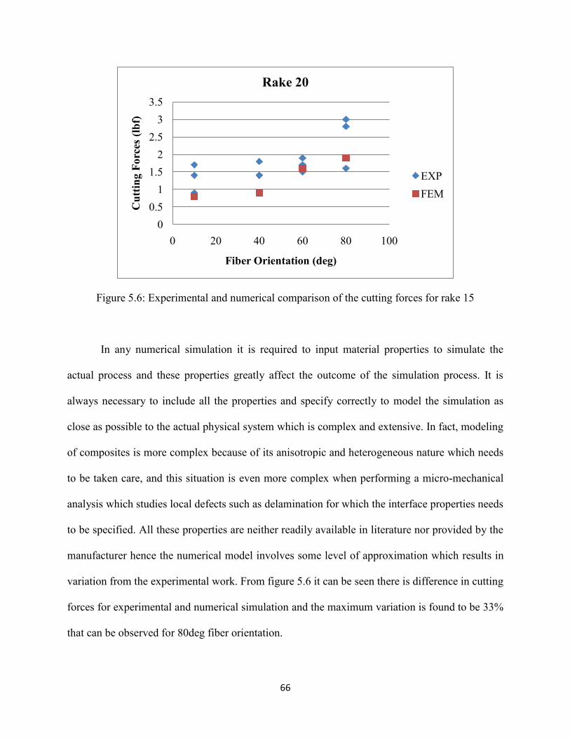
66

Figure 5.6: Experimental and numerical comparison of the cutting forces for rake 15

In any numerical simulation it is required to input material properties to simulate the

actual process and these properties greatly affect the outcome of the simulation process. It is

always necessary to include all the properties and specify correctly to model the simulation as

close as possible to the actual physical system which is complex and extensive. In fact, modeling

of composites is more complex because of its anisotropic and heterogeneous nature which needs

to be taken care, and this situation is even more complex when performing a micro-mechanical

analysis which studies local defects such as delamination for which the interface properties needs

to be specified. All these properties are neither readily available in literature nor provided by the

manufacturer hence the numerical model involves some level of approximation which results in

variation from the experimental work. From figure 5.6 it can be seen there is difference in cutting

forces for experimental and numerical simulation and the maximum variation is found to be 33%

that can be observed for 80deg fiber orientation.

00.5

11.5

22.5

33.5

0 20 40 60 80 100

Cut

ting

Forc

es (l

bf)

Fiber Orientation (deg)

Rake 20

EXPFEM

67

5.7 Delamination length

The finite element analysis was run on a unidirectional material with mechanical

properties given in table 5.1 and the delamination lengths for different fiber orientation are

shown in figure 5.7 to 5.10. Once the cutting is done the fibers will spring back to its original

position due to elastic recovery and looks very normal without delamination but, there still exists

delamination which has to be clearly investigated by going back and checking at different time

frames.

Since composites are widely used in aviation industry, delamination causes a serious

threat for its service life. The delamination zone provides an opportunity for impurities to sneak

through, particularly moisture which at room temperature doesn‟t cause a serious problem but

when the aircraft is flying at high altitudes during service, water freezes to form ice and due to

volumetric expansion the separation between fibers and matrix increase thereby causing severe

delamination issue during its operation and deteriorating its structural integrity.

Figure 5.7: Delamination damage for 80deg fiber orientation

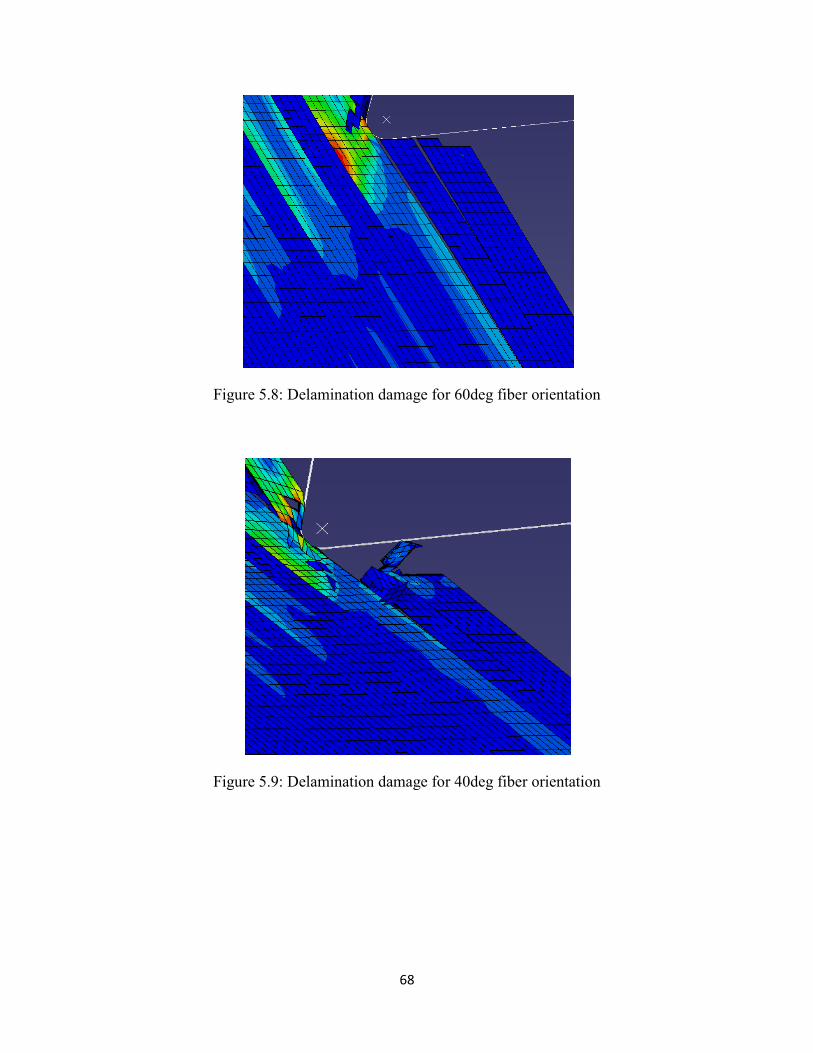
68



69


Figures 5.7 to 5.10 clearly shows the delamination for 80, 60, 40 and 10deg respectively,

the delamination lengths is measured by selecting a node on the desired fiber along the trim

plane and selecting another node along fiber axis up to the point of maximum separation for

which the software measures the shortest distance measuring delamination length.

70

CHAPTER VI

RESULTS AND DISCUSSION

The orthogonal experimental and numerical cutting forces with respect to fiber

orientations on NPT material is plotted for different rake angles. Figure 6.1 to 6.4 represent the

cutting force for 5, 10, 15 and 20deg respectively with other parameters kept constant.

Figure 6.1: Experimental and numerical cutting forces for rake 5deg on NPT material

From figure 6.1 it can be seen that the cutting forces increases both in experiments and

numerical simulations as the fiber orientation increases and this is because the failure mode

changes from mode I to mode III as explained in chapter three. Even though there is a large

variation in certain experimental and numerical values but follows the same trend indicating the

correctness of the numerical model, the larger experimental cutting forces might be attributed to

tool wear.

012345678

0 20 40 60 80 100

Cut

ting

Forc

es (l

bf)


Rake 5

EXPFEM

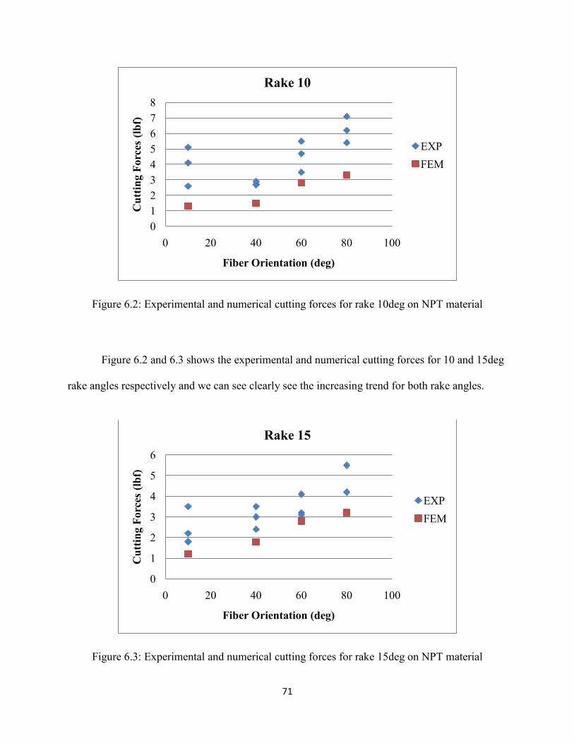
71


Figure 6.2 and 6.3 shows the experimental and numerical cutting forces for 10 and 15deg

rake angles respectively and we can see clearly see the increasing trend for both rake angles.


012345678

0 20 40 60 80 100

Cut

ting

Forc

es (l

bf)


Rake 10

EXPFEM

0

1

2

3

4

5

6

0 20 40 60 80 100

Cut

ting

Forc

es (l

bf)


Rake 15

EXPFEM

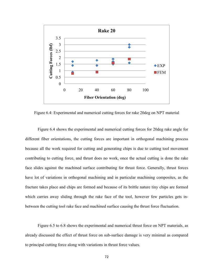
72


Figure 6.4 shows the experimental and numerical cutting forces for 20deg rake angle for

different fiber orientations, the cutting forces are important in orthogonal machining process

because all the work required for cutting and generating chips is due to cutting tool movement

contributing to cutting force, and thrust does no work, once the actual cutting is done the rake

face slides against the machined surface contributing for thrust force. Generally, thrust forces

have lot of variations in orthogonal machining and in particular machining composites, as the

fracture takes place and chips are formed and because of its brittle nature tiny chips are formed

which carries away sliding through the rake face of the tool, however few particles gets in-

between the cutting tool rake face and machined surface causing the thrust force fluctuation.

Figure 6.5 to 6.8 shows the experimental and numerical thrust force on NPT materials, as

already discussed the effect of thrust force on sub-surface damage is very minimal as compared

to principal cutting force along with variations in thrust force values.

00.5

11.5

22.5

33.5

0 20 40 60 80 100

Cut

ting

Forc

es (l

bf)


Rake 20

EXPFEM

73

Figure 6.5: Experimental and numerical thrust forces for rake 5deg on NPT material


Figure 6.6 and 6.7 shows the plot of thrust force and fiber orientations for 5 and 10deg

respectively, the thrust forces doesn‟t follow any particular trend a values were randomly

distributed which is normal and observed in prior literature.

0

1

2

3

4

5

6

0 20 40 60 80 100

Thr

ust F

orce

s (lb

f)


Rake 5

EXPFEM

00.5

11.5

22.5

33.5

4

0 20 40 60 80 100

Thr

ust F

orce

s (lb

f)


Rake 10

EXPFEM

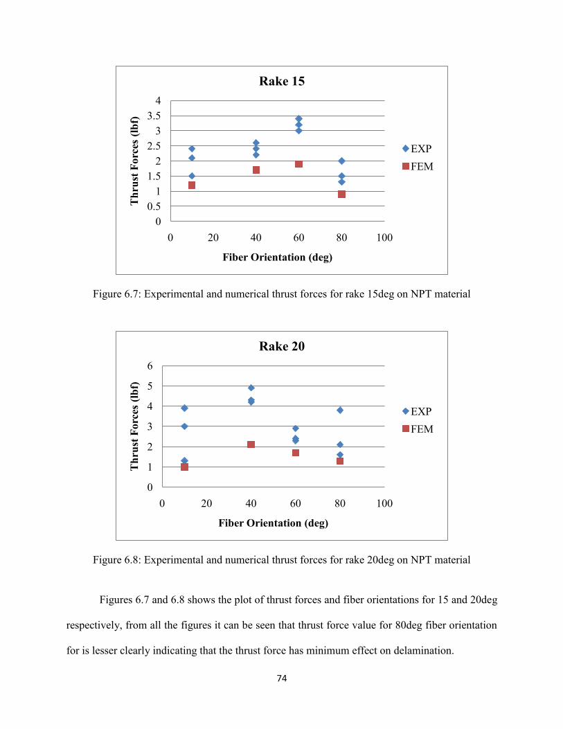
74



Figures 6.7 and 6.8 shows the plot of thrust forces and fiber orientations for 15 and 20deg

respectively, from all the figures it can be seen that thrust force value for 80deg fiber orientation

for is lesser clearly indicating that the thrust force has minimum effect on delamination.

00.5

11.5

22.5

33.5

4

0 20 40 60 80 100

Thr

ust F

orce

s (lb

f)


Rake 15

EXPFEM

0

1

2

3

4

5

6

0 20 40 60 80 100

Thr

ust F

orce

s (lb

f)


Rake 20

EXPFEM

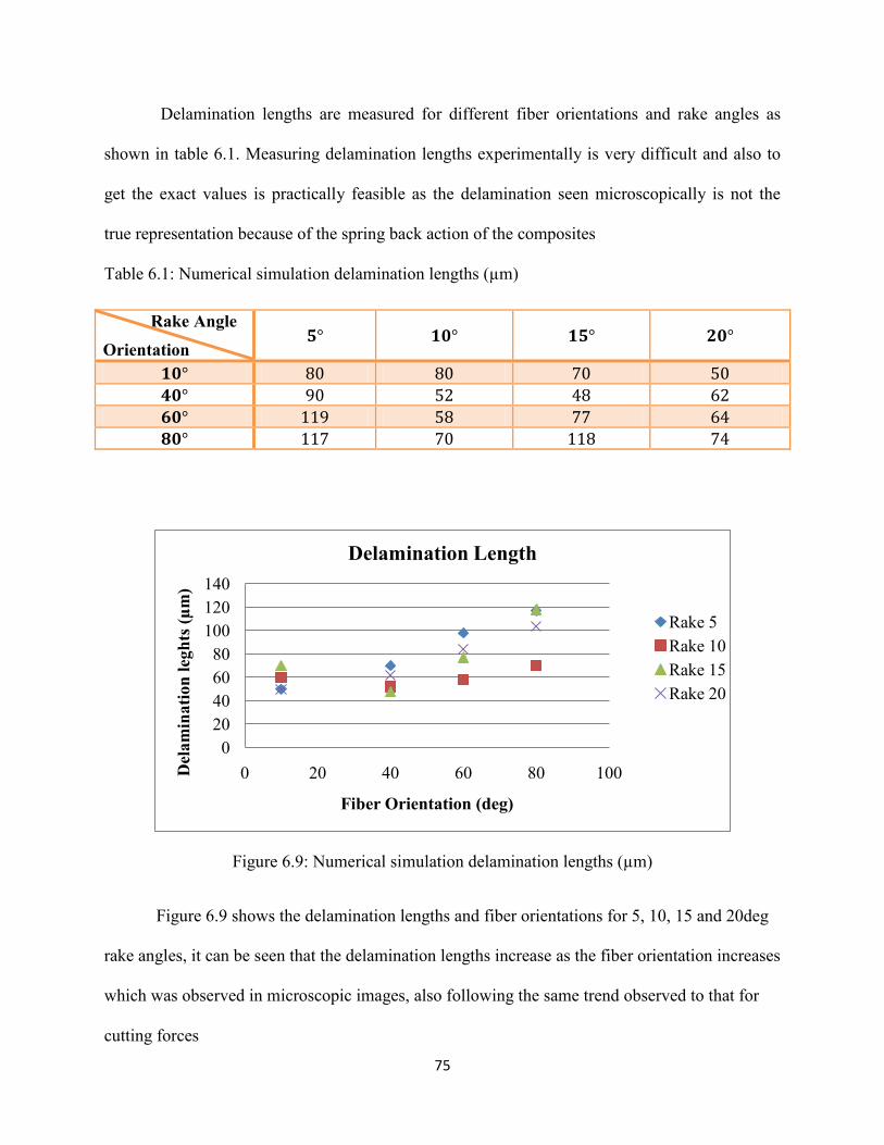
75

Delamination lengths are measured for different fiber orientations and rake angles as

shown in table 6.1. Measuring delamination lengths experimentally is very difficult and also to

get the exact values is practically feasible as the delamination seen microscopically is not the

true representation because of the spring back action of the composites

Table 6.1: Numerical simulation delamination lengths (µm)


Figure 6.9: Numerical simulation delamination lengths (µm)

Figure 6.9 shows the delamination lengths and fiber orientations for 5, 10, 15 and 20deg

rake angles, it can be seen that the delamination lengths increase as the fiber orientation increases

which was observed in microscopic images, also following the same trend observed to that for

cutting forces

020406080

100120140

0 20 40 60 80 100Del

amin

atio

n le

ghts

(µm

)


Delamination Length

Rake 5Rake 10Rake 15Rake 20

76

CHAPTER 7

CONCLUSION AND FUTURE WORK

7.1 Conclusion

Orthogonal machining was experimentally conducted for different positive fiber

orientations and rake angles and compared with numerical simulation and found to be in good

agreement.

A new modeling technique to predict delamination is presented here that specifies surface

based cohesive behavior for interactions between 3D fibers and matrix without actually creating

a layer for cohesive zone used in prior literature, thereby creating a more realistic model to

predict delamination and also accounting for accurate volume ratios.

The surface quality does not always decrease with increasing positive fiber orientation

and was found the better quality is obtained for 0 and 40deg fiber orientation. Also, the effect of

rake angle is high for fiber orientation 60 and 80deg, where as it is negligible for 10 and 40deg.

The surface quality rapidly decreases for 60deg when compared to 40deg fiber orientation due to

chip formation mechanisms.

Delamination lengths were measured from numerical simulations and found to have the

most damage for 80deg fiber orientation indicating a good agreement with experimental

machining.

77

7.2 Future Work

In the future, each lamina can also be modeled using two phase system of fiber and

matrix in the depth direction, so that each fiber will be completely surrounded by matrix

representing actual composite panel, but will drastically increase the contacts defined and

computational time.

Also a full factorial study can be conducted to investigate the effect of machining

conditions and cutting tool parameters on delamination depth to study their behavior and come

up with optimized process parameters.

Frictional forces vary with fiber orientation and increases with increasing fiber

orientation. Numerical simulations can be performed with different friction coefficients

depending on fiber orientations to investigate their effects on delamination damage and cutting

forces.

78

REFERENCES

79

REFERENCES

[1] A. Koplev, Lystrup, & T. Vorm, (1983) „The cutting process, chips, and cutting forces in machining CFRP‟ Composites 14 p371-376.

[2] N. Bhatnagar, N. Ramakrishnan, N. K. Naik and R. Komanduri, (1995) „On the

machining of fiber reinforced plastic (FRP) composite laminate‟ Int. J of Mach. Tools & Manufacture 35 p701-716.

[3] X. M. Wang & L. C. Zhang, (2003) „An experimental investigation into the orthogonal

cutting of unidirectional fiber reinforced plastics‟ Int. J of Mach. Tools & Manufacture 43 p1015-1022.

[4] D. H. Wang, M. Ramulu & D. Arola, (1995) „Orthogonal cutting mechanisms of

graphite/epoxy composite. Part I unidirectional laminate‟ Int. J of Mach. Tools & Manufacture, 35 p1623-1638.

[5] Mkaddem, A., Demirci, I., El Mansori, M., (2008), „A Micro–Macro Combined Approach

Using FEM for Modelling of Machining of FRP Composites Cutting Forces Analysis‟, Composites Science and Technology, 68 p3123-3127.

[6] L. C. Zhang, H. J. Zhang & X. M. Wang, (2001) ‘A force prediction model for cutting

uni-directional fiber-reinforced plastics‟ Machining Science and Technology 5 p293-305. [7] Jamal Sheikh Ahmad, „Machining of polymer composites‟ Springer (2008) pp230 ISBN

978-0-387-35539-9. [8] G. C. Everstein and T. G. Rogers., (1971) „A Theory of Machining Fiber-Reinforced

Materials‟, Journal of Composite Materials. 5 p94-106. [9] J. F. Mulhern, T. G. Rogers and A. J. M. Spencer, (1967) „A Continuum Model for Fiber

Reinforced Plastic Materials‟, International Journal of Engineering Sciences. 7 p473 – 492.

[10] W. B. Palmer, P. L. B. Oxley. (1989) „Mechanics of Orthogonal Machining‟, Proc. Inst.

Mech. Engrs. 173 p623-654. [11] A. C. Pipkin and T. G. Rogers, (1971) „Plane Deformation of Incompressible Fiber

Reinforced Materials‟, Tran of ASME, Journal of Applied Mechanics. p630-640. [12] A. Koplev, (1980) „Cutting of CFRP with single edge tools‟, 3rd International Conference

on Composite Materials, Paris. [13] H. Inoue, and M. Ido, (1986) „Study on the cutting mechanism of GFRP‟. In Proceedings

of International Symposium on Composite Materials and Structures, Beijing, China.

80

[14] H. Takeyama and N. Iijima, (1988) „Machinability of Grass Fiber Reinforced Plastics and Application of Ultrasonic Machining‟, Annals of CIRP, 37 p93-96.

[15] Venu Gopala Rao, G., Mahajan, P., Bhatnagar, N., (2007) „Micro-Mechanical Modeling

of Machining of FRP Composites – Cutting Force Analysis‟, Composites Science and Technology, 67 p579-593.

[16] D. Walrath, and D. Adams, (1987). „Current status of the Iosipescu shear test method‟,

Journal of Composite Materials, 21 p494-507. [17] D. Wang, M. Ramulu, and D. Arola, (1995). „Orthogonal cutting mechanisms of

graphite/epoxy composite. Part-1 Unidirectional laminate‟. International Journal of Machine Tools and Manufacturing. 35 p1639-1648.

[18] D. Arola, and M. Ramulu, (1997) „Orthogonal cutting of fiber reinforced composite a

finite element analysis‟, International Journal of Mechanical Science. 37 p597-613. [19] M. V. Ramesh, K. N. Seetharamu, N. Ganesan and M. S. Sivakumar, (1998) „Analysis of

machining of FRPs using FEM‟, International Journal of Machine Tools and Manufacture. 38, p1531-1549.

[20] D. Arola, M. B. Sultan and M. Ramulu, (2002) „Finite element modeling of edge trimming

fiber reinforced plastics‟, Transactions of the ASME, 124 p32-41. [21] R. M. Jones, (1975), „Mechanics of Composite Materials‟, McGraw-Hill, Washington,

D.C. [22] S. Valliappan, P. Boonlaulohr, I. K. Lee, (1976) „Non-linear analysis of fibrous

composite structures a plasticity approach‟, International Journal of Numerical Methods in Engineering, 10 p597-606.

[23] M. Mahdi and L. Zang, (2001) “An adaptive three-dimensional finite element algorithm

for the orthogonal cutting of composite materials”, Journal of Materials Processing Technology, 113 p368-372.

[24] M. Mahdi and L. Zang, (2001) „A finite element model for the orthogonal cutting of fiber-

reinforced composite materials‟, Journal of Materials Processing Technology, 113 p373-377.

[25] A. Sahraie-Jahromi, G. Chennakesavelu, G. Gudimani, and B. Bahr, (2009) „Study of

Damaged Area in Drilling of Composites with DOE analysis‟, in SAMPE 09, Baltimore, MD, USA.

[26] Nayak, D., Bhatnagar, N., Mahajan, P., (2005) „Machining Studies of UD-FRP

Composites Part 2 Finite Element Analysis‟, Machining Science and Technology, 9 p503-528.

orthogonal machining of uni-directional carbon fiber

Documents