NBER WORKING PAPER SERIES

ORIGINS OF STOCK MARKET FLUCTUATIONS

Daniel L. GreenwaldMartin Lettau

Sydney C. Ludvigson

Working Paper 19818http://www.nber.org/papers/w19818

NATIONAL BUREAU OF ECONOMIC RESEARCH1050 Massachusetts Avenue

Cambridge, MA 02138January 2014

The authors are grateful to Jarda Borovicka and Eric Swanson for helpful comments. The views expressedherein are those of the authors and do not necessarily reflect the views of the National Bureau of EconomicResearch.

NBER working papers are circulated for discussion and comment purposes. They have not been peer-reviewed or been subject to the review by the NBER Board of Directors that accompanies officialNBER publications.

© 2014 by Daniel L. Greenwald, Martin Lettau, and Sydney C. Ludvigson. All rights reserved. Shortsections of text, not to exceed two paragraphs, may be quoted without explicit permission providedthat full credit, including © notice, is given to the source.

Origins of Stock Market FluctuationsDaniel L. Greenwald, Martin Lettau, and Sydney C. LudvigsonNBER Working Paper No. 19818January 2014, Revised April 2014JEL No. G0,G12

ABSTRACT

Three mutually uncorrelated economic shocks that we measure empirically explain 85% of the quarterlyvariation in real stock market wealth since 1952. We use a model to show that they are the observableempirical counterparts to three latent primitive shocks: a total factor productivity shock, a risk aversionshock that is unrelated to aggregate consumption and labor income, and a factors share shock thatshifts the rewards of production between workers and shareholders. On a quarterly basis, risk aversionshocks explain roughly 75% of variation in the log difference of stock market wealth, but the near-permanentfactors share shocks plays an increasingly important role as the time horizon extends. We find thatmore than 100% of the increase since 1980 in the deterministically detrended log real value of thestock market, or a rise of 65%, is attributable to the cumulative effects of the factors share shock, whichpersistently redistributed rewards away from workers and toward shareholders over this period. Indeed,without these shocks, today's stock market would be about 10% lower than it was in 1980. By contrast,technological progress that rewards both workers and shareholders plays a smaller role in historicalstock market fluctuations at all horizons. Finally, the risk aversion shocks we identify, which are uncorrelatedwith consumption or its second moments, largely explain the long-horizon predictability of excessstock market returns found in data. These findings are hard to reconcile with models in which time-varyingrisk premia arise from habits or stochastic consumption volatility.

Daniel L. GreenwaldDepartment of EconomicsNew York University19 West 4th Street, 6th floorNew York, NY 10012dlg340@nyu.edu

Martin LettauHaas School of BusinessUniversity of California, Berkeley545 Student Services Bldg. #1900Berkeley, CA 94720-1900and NBERlettau@haas.berkeley.edu

Sydney C. LudvigsonDepartment of EconomicsNew York University19 W. 4th Street, 6th FloorNew York, NY 10002and NBERsydney.ludvigson@nyu.edu

1 Introduction

Asset pricing theorists have long been concerned with explaining stock market expected

returns, typically measured over monthly, quarterly or annual horizons. This is important

because empirical evidence suggests that variation in the stock market price-dividend ratio

is driven almost entirely by expected excess return variation (i.e., forecastable movements

in equity premia).1 Far less attention has been given to understanding the real (adjusted

for in�ation) level of the stock market, i.e., stock price variation, or the cumulation of

returns over many decades. The profession spends a lot of time debating which risk factors

drive expected excess returns, but little time investigating why real stock market wealth has

evolved to its current level compared to 30 years ago. To understand the latter, it is necessary

to probe beyond the role of stationary risk factors and short-run expected returns, to study

the primitive economic shocks from which all stock market (and risk factor) �uctuations

originate.

To see why, consider that some economic shocks may have tiny innovations but permanent

or near-permanent e¤ects on cash �ows. Under rational expectations, permanent cash �ow

shocks have no in�uence on the price-dividend ratio (they are incorporated immediately

into both prices in the numerator and dividends in the denominator), but they can have a

dramatic in�uence on real stock market wealth as the decades accumulate. Such shocks are

the sources of stochastic trends in stock prices that are by de�nition impossible to predict

and not re�ected in expected returns. On the other hand, �uctuations in expected returns

may be associated with movements in risk premia and can persistently shift the real value of

the stock market around its long-term trend. But because these �uctuations are transitory,

their impact eventually dies out. Stock market wealth evolves over time in response to the

cumulation of both transitory expected return and permanent cash �ow shocks. The crucial

unanswered questions are, what are the economic sources of these shocks? And what have

been their relative roles in evolution of the stock market over time?

The objective of this paper is to address these questions. We begin by identifying three

mutually orthogonal observable economic shocks that explain the vast majority (over 85%)

of quarterly �uctuations in real stock market wealth since the early 1950s. Econometrically,

these shocks are measured as speci�c orthogonal movements in consumption, labor income,

and asset wealth (net worth), identi�ed from a cointegrated vector autoregression (VAR)

and extracted using a standard recursive identi�cation procedure. Roughly speaking, this

1Expected dividend growth and expected short-term interest rates play little role empirically in price-dividend ratio variation (Campbell (1991); Cochrane (1991); Cochrane (2005); Cochrane (2008)).

1

methodology decomposes movements in log stock market wealth into those associated with

(1) shocks to log aggregate consumption, (2) shocks to the log labor income-consumption

ratio, holding �xed consumption, and (3) shocks to log stock wealth holding �xed both log

consumption and log labor income. We investigate how these shocks have a¤ected stock

market wealth over time, with special attention paid to their relative importance over short

versus long time horizons.

We then address the question of what these observable VAR shocks represent economi-

cally. Providing an economic interpretation of the shocks requires a theoretical framework.

A common theoretical approach for explaining stock market behavior is to assume the ex-

istence of a representative agent who consumes the aggregate consumption stream.2 But

we �nd that understanding the observable sources of variation we �nd in stock prices in

post-war data drives us to consider a framework with heterogeneity. So this paper devel-

ops a general equilibrium model of two types of agents: shareholders and workers. The

representative shareholder in the model is akin to a large institutional investor or wealthy

individual who derives all income from investments. The representative worker consumes

a stream of labor income every period. Economic �uctuations in the model originate from

three mutually orthogonal primitive shocks that di¤erentially a¤ect each type: a permanent

total factor productivity (TFP) shock that governs the state of factor neutral technological

progress and propels aggregate (shareholder plus worker) consumption, a near-permanent

factor shares shock that reallocates the rewards from production between shareholders and

workers without a¤ecting the size of those rewards, and an independent shock to shareholder

risk aversion that moves the stochastic discount factor pricing assets independently of stock

market fundamentals or real variables such as consumption and labor income. The modi�er

�independent� in reference to shareholder risk aversion refers to the independence in the

model of such shocks from macroeconomic fundamentals (dividends, earnings, consumption,

labor income, output). Our �ndings indicate that this independence is essential for explain-

ing the observed time-variation in the reward for bearing stock market risk, implying that

quantitatively large component of risk premia �uctuations is acyclical. One interpretation

of this is that risk premia are driven by intangible information that is largely unrelated to

the current economic state. In this sense, our �ndings contrast with classic earlier studies

that emphasized the countercyclicality of risk premia (e.g., Fama and French (1989)). We

discuss this further below.

2This approach is widely taken, including among the leading asset pricing theories of the day. In�uentialexamples include Campbell and Cochrane (1999) and Bansal and Yaron (2004).

2

The model is then employed to show that the mutually orthogonal VAR innovations that

explain almost all stock market variation are the observable empirical counterparts to the

latent primitive shocks in the theoretical framework. Speci�cally, we show that, if the model

generated the data, the total factor productivity shock would be revealed as a consumption

shock in the VAR, namely a movement in log consumption, ct, that contemporaneously

a¤ects both log labor income, yt, and log asset wealth, at, where all three move in the same

direction. The factors share shock would be revealed as a labor income shock that moves at in

the opposite direction of yt but is restricted to have no contemporaneous impact on ct. And

the risk aversion shock would be revealed as a wealth shock that moves at but is restricted

to have no contemporaneous impact on either ct or yt. We show that the dynamic responses

to these mutually orthogonal VAR innovations produced from model generated data are

remarkably similar to those produced from historical data. We refer to the three mutually

orthogonal VAR innovations (consumption, labor income and wealth) interchangeably as

productivity or TFP, factors share, and risk aversion innovations, respectively.

How have these shocks a¤ected stock market wealth over time? We �nd that the vast

majority of short- and medium-term stock market �uctuations in historical data are driven

by risk aversion shocks, revealed as movements in wealth that are orthogonal to consumption

and labor income, both contemporaneously (an identifying assumption), and at all subse-

quent horizons (a result). Although transitory, these shocks are quite persistent with a half

life of over four years. On a quarterly basis, they explain approximately 75% of variation

in the log di¤erence of stock market wealth, but their contribution declines as the horizon

extends. These facts are well explained by the model, in which the orthogonal wealth shocks

originate from independent shifts in investors� willingness to bear risk.

At longer horizons, the relative importance of the shocks changes. The factors share shock

explains a negligible fraction of variation in the stock market over shorter time horizons, but

because its innovations are nearly permanent, it plays an increasingly important role as the

time horizon extends. A spectral decomposition of variance by frequency shows that this

shock explains virtually none of the variation in the real level of the stock market over cycles

of a quarter or two, but it explains roughly 40% over cycles two to three decades long.

These facts are well explained by the model economy, which is subject to small but highly

persistent innovations that shift the allocation of rewards between shareholders and workers

independently from the magnitude of those rewards.

By contrast, factor neutral productivity shocks, revealed as consumption shocks empiri-

cally, play a small role in the stochastic �uctuations of the stock market at all horizons, once

3

a deterministic trend is removed. The model is consistent with this �nding. The crucial

aspect of the model that makes it consistent with this �nding is its heterogeneous agent

speci�cation: given capital�s smaller role in the production process, most gains and losses

from total factor productivity shocks accrue to workers rather than shareholders, so their

e¤ect on stock market wealth is smaller than that of the other two shocks. This �nding is

a direct contradiction of representative agent asset pricing models where shocks that drive

aggregate consumption plays a central role in stock market �uctuations.

As an example of the magnitude of these forces for the long-run evolution of the stock

market, we decompose the percent change since 1980 in the deterministically detrended

real value of stock market wealth that is attributable to each shock. The period since

1980 is an interesting one to consider, in which the cumulative e¤ect of the factor shares

shock persistently redistributed rewards away from workers and toward shareholders. (The

opposite occurs from the mid 1960s to mid 1980s.) After removing a deterministic trend, we

�nd that the cumulative e¤ects of the factors share shocks have resulted in a 65% increase in

real stock market wealth since 1980, an amount equal to 110% of the total increase in stock

market wealth over this period. Indeed, without these shocks, today�s stock market would

be roughly 10% lower than it was in 1980. This �nding underscores the extent to which the

long-term value of the stock market has been profoundly altered by forces that reallocate

the rewards of production, rather than raise or lower all of them.

Our calculations imply that an additional 38% of the increase in the detrended real value

of the stock market since 1980, or a rise of 22%, is attributable to the cumulative e¤ects

of risk aversion shocks, which were on average lower in the last 30 years than earlier in the

post-war period. By contrast, the cumulative e¤ects of TFP shocks have made a negative

contribution to change in stock market wealth since 1980, once a deterministic trend is

removed. The importance of the TFP shock is uncharacteristically large over this period,

a direct consequence of the string of unusually large negative draws for consumption in

the Great Recession years from 2007-2009. These shocks account for -38% of the increase

since 1980. Together, the three mutually orthogonal economic shocks we identify explain

almost all of the increase in deterministically detrended real stock market wealth since 1980.

(Speci�cally, they account for 110% of the increase, with the remaining -10% accounted for

by a residual.)

Finally, our �ndings speak to the question of why the stock market is predictable. The

process for shareholder risk aversion in the model is highly non-linear, with shareholders

close to risk-neutral most of the time but subject to rare �crises� in their willingness to bear

4

risk, captured in the model by infrequent, large spikes in risk aversion. These states lead

to rare ��ights to safety� in which the market crashes. Below we explain why this strong

non-linearity is important for simultaneously matching the range of empirical evidence we

study here. But even in normal times, the time-varying expectation that risk tolerance

could crash in the future generates continuous �uctuations in the price-dividend ratio that

are associated with forecastable variation in excess stock market returns, or a time-varying

equity risk premium. Risk premia variation is observable as the orthogonal wealth shocks

from the empirical VAR, which in turn generate excess return predictability in a linear

forecasting regression. This model implication is closely matched in the data. In particular,

the predictive content for long horizon excess stock market returns of common stock market

forecasting variables (such as the price-dividend ratio or cayt) is found to be largely subsumed

by the information in lags of the independent risk aversion/wealth shock. These variables

forecast excess returns only because they are correlated with the VAR wealth shocks.

An important aspect of these results is that the time-variation in the reward for bearing

risk, both in the model and the data, is divorced from �uctuations in traditional macro-

economic fundamentals. The wealth shocks we identify are by construction orthogonal to

movements in consumption and labor income contemporaneously, and, as we show, at all

future horizons (a result).We also �nd that these innovations bear little relation to other tra-

ditional macroeconomic fundamentals such as dividends, earnings, consumption volatility, or

broad-based macroeconomic uncertainty, and none of these variables forecast equity premia.

These �ndings are hard to reconcile with models in which time-varying risk premia arise from

habits (which vary with innovations in consumption), stochastic consumption volatility, or

consumption uncertainty.

These �ndings are consistent with other theories in which time-variation in risk premia

is largely divorced from �uctuations in macroeconomic fundamentals and instead associated

with independent market crises. Examples include the ambiguity aversion framework of

Bianchi, Ilut, and Schneider (2013), in which a component of investor con�dence varies in

a manner like our risk aversion that is independent of shocks to economic fundamentals,

or intermediary-based models in which intermediaries� risk-bearing capacity varies indepen-

dently of macroeconomic fundamentals (e.g., Gabaix and Maggiori (2013)), or models where

restrictions on intermediaries risk-bearing capacity result in very strong nonlinearities be-

tween risk premia and macroeconomic state variables (e.g., Brunnermeier and Sannikov

(2012); He and Krishnamurthy (2013); Muir (2014)).3 Of course, the intermediaries� risk-

3In general these non-linearities must be quite extreme. In the model studied here, the extreme non-

5

bearing capacity could itself be driven by �uctuations in the risk or ambiguity aversion of

households who ultimately supply intermediaries with capital. We view the evidence pre-

sented here as contributing to a growing body that narrows the class of plausible explanations

for time-varying risk premia to those that are not primarily driven by shocks to traditional

economic fundamentals. We discuss this further in the conclusion.

This empirical part of this paper builds on Lettau and Ludvigson (2013). That paper

provided empirical evidence in a purely statistical model, studying (a rotation of) the three

VAR innovations described here and their relationship to di¤erent components of household

wealth, consumption and labor income. The main contribution of this paper is to provide an

economic interpretation of these innovations and a detailed investigation of their implications

for the stock market. Our model is also related to the work of several recent papers that have

emphasized the weak empirical correlation between stock market behavior and innovations to

consumption growth or its second moments (Du¤ee (2005), Albuquerque, Eichenbaum, and

Rebelo (2012), Lettau and Ludvigson (2013)). And there is an important earlier literature

in asset pricing that identi�ed and distinguished cash-�ow from discount rate �shocks� (e.g.,

Campbell (1991); Cochrane (1991)). This work was central to our understanding of how

innovations in stock returns are related to forecastable movements in returns as compared

to dividend growth, but it is silent on the underlying economic mechanisms that drive these

forecastable changes. It is precisely these primitive economic shocks that are the subject of

this paper.

The rest of this paper is organized as follows. The next section describes the econometric

procedure and data used to identify the three mutually uncorrelated empirical shocks from

a VAR on consumption, labor income, and asset wealth. Section 3 describes the theoretical

model that we use to interpret these shocks. Section 4 presents our �ndings, which are of two

forms. The �rst are results on the performance of the model, including summary statistics

for standard asset pricing implications. This section also demonstrates that the mutually

orthogonal VAR innovations described in Section 3 are the observable empirical counterparts

to the latent primitive shocks in the model. The second set of results studies the relative

role of the observable shocks in historical stock market �uctuations, with special attention

paid to how these roles depend on the time horizon over which one measures a change in

stock market wealth. Here we compare the role of each shock in the dynamic responses

linearity of risk aversion is enough to explain why �uctuations in risk premia appear largely divorced frommacroeconomic fundamentals even when we force the risk-aversion shock to be perfectly negatively correlatedwith the TFP shock. But, as we explain below, it is very di¢cult to match the full range of evidence presentedhere without an independent shock to risk aversion.

6

and variance decompositions of stock market wealth when estimated from historical data

with the same statistics when estimated from model-generated data and show that they

are remarkably similar along a number of dimensions discussed below. The �nal subsection

investigates the question of why stock returns are predictable. We show that the independent

risk aversion shocks we identify largely explain why long-horizon excess stock market returns

are predictable by common forecasting variables such as the log price-dividend ratio or the

consumption-wealth variable cayt. Section 6 brie�y discusses the link between the factors

share shock and economic inequality. Section 7 concludes.

2 Econometric Analysis: Three Mutually Orthogonal Shocks

This section describes the empirical analysis used to identify three mutually orthogonal

observable shocks from data on aggregate consumption, labor income and household wealth.

2.1 Data

Many empirical details of the estimation that follows are covered in Lettau and Ludvigson

(2013). Here we outline the main elements and refer the reader to that paper for more

information.4

We consider a cointegrated vector of variables in the data, denoted xt = (ct; yt; at)0,

where ct is log of real, per capita aggregate consumption, yt is log of real, per-capita labor

income, and at is log of real, per-capita asset wealth. Throughout this paper we use lower

case letters to denote log variables, e.g., ln (At) � at: Lettau and Ludvigson (2013) provide

updated evidence of a cointegrating relation among these variables, which can be motivated

by considering the long-run implications of a standard household budget constraint (see

Lettau and Ludvigson (2001)).

The Appendix contains a detailed description of the data used in this study. The log

of asset wealth, at; is a measure of real, per capita household net worth, which includes all

�nancial wealth, housing wealth, and consumer durables. It is compiled from the �ow of

funds accounts by the Board of Governors of the Federal Reserve.

We study the implications of the empirical shocks identi�ed from the system (ct; yt; at)0

and subsequently relate these shocks to stock market wealth. We denote the log of stock

4That paper showed how the innovations we study here can be econometrically identi�ed as disturbancesdistinguished by whether their e¤ects are permanent or transitory. An additional rotation of innovations wasrequired for this interpretation, but the shocks obtained there are perfectly correlated with those obtainedhere and discussed below.

7

market wealth st: Stock market wealth is a component of total asset wealth. Corporate

equity was 23% of total asset wealth in 2010, and 29% of net worth. For comparison, we

will often also study the implications of these same shocks for the Center for Research in

Securities Prices (CRSP) value-weighted stock price index. We denote the log of the CRSP

value-weighted stock price index pt.

We use the log of real, per capita, expenditures on nondurables and services (excluding

shoes and clothing), as a measure of ct. From the household�s budget constraint, an internally

consistent cointegrating relation among ct, yt, and at, may then be obtained if we assume

that the log of (unobservable) real total �ow consumption is cointegrated with the log of real

nondurables and services expenditures (Lettau and Ludvigson (2010)). The log of after-tax

labor income, yt, is also measured in real, per capita terms. Lettau and Ludvigson (2013)

presents empirical evidence supportive of a single cointegrating relationships between ct, at,

and yt in the post-war data used in the study.5 Our data are quarterly and span the �rst

quarter of 1952 to the third quarter of 2012.

2.2 Empirical Implementation

Before explaining the details of the estimation, we discuss a practical distinction between

the data and the model. The model developed below is intended to focus on the implications

of the empirical shocks for stock market wealth. As such, it has one form of risky capital

(equity) and a risk-free bond in zero net supply. It follows that, in the model, all wealth is

stock market wealth, which is the same as total wealth, which is the same as net worth. In

historical data, total wealth contains non-equity forms of wealth, so total wealth and stock

market wealth are two di¤erent variables. As noted above, stock market wealth accounts for

about 23% of total wealth in 2010. In the data we distinguish the two by denoting log of

asset wealth (net worth) by at and log of stock market wealth by st: In the model, at = st:

In constructing the empirical VAR innovations discussed next, we use system of variables

that contains consumption, labor income and total asset wealth at, and then subsequently

5The data provide no evidence of a second linearly independent cointegrating relation (there can be atmost two). In particular, bivariate log ratios of these variables appear to contain trends in our sample.Economic models often imply that bivariate log ratios (e.g., yt � at) are stationary, and the model belowassumes as much. In �nite samples, it is impossible to distinguish a highly persistent but stationary seriesfrom a non-stationary one. For the empirical system, we follow the advice of Campbell and Perron (1991)and empirically model only the single, trivariate cointegrating relation for which we �nd direct statisticalevidence of in our sample. For the model, we set parameter values that imply the log ratio yt � at isstationary but deviations from the common trend in yt and at are so persistent one could not reject a unitroot in samples of the size we currently face, consistent with the data.

8

relate these innovations to stock market wealth. We do not construct these innovations

by restricting analysis to how consumption and labor income move only with stock market

wealth. We do this for two reasons. First, a (factor neutral) TFP shock should a¤ect the

value of all productive capital, so a system that identi�es such a shock from the data should

include total wealth. If TFP shocks a¤ect non-stock wealth but these components are omitted

from the system, this could lead to spurious estimates of productivity and its dynamics,

which would also contaminate estimates of the factors share and risk aversion shocks that

are presumed orthogonal to the TFP shock. Second, consumption and labor income are

cointegrated with total wealth, as expected from theory (Lettau and Ludvigson (2001)), but

there is no implication that these variables should be (or are) cointegrated with stock market

wealth by itself, a component of total wealth. It is important to control empirically for these

long-run relationships by imposing the restrictions implied by cointegration in a VAR for

which wealth shares a common trend with consumption and labor income. When this is

done, it will then be an empirical matter how closely the identi�ed VAR shocks are related

to stock market wealth, which is the subject of an extensive investigation below. Notice

that there is no implication that the shocks identi�ed from the ct: yt; at empirical system

should explain all or even most of the variation in stock market wealth st. Although st can

be related to these shocks, there will be an unexplained residual that in principal could be

quite important, as we explain below.

Identi�cation of the three mutually orthogonal empirical disturbances is achieved in sev-

eral steps. First, we assume all of the series contained in xt are �rst order integrated, or

I(1), an assumption con�rmed by unit root tests, available upon request. The cointegrat-

ing coe¢cient on consumption is normalized to one, and we denote the single cointegrating

vector for xt = [ct; at; yt]0 as � = (1;��a;��y)0. The cointegrating parameters �a and �y

are estimated using dynamic least squares, which generates �superconsistent� estimates of

�a and �y (Stock and Watson, 1993).6 We estimate b� = (1;�0:18;�0:70)0: The Newey and

West (1987) corrected t-statistics for these estimates are 20 and 56, respectively.

Second, a cointegrated VAR (or vector error correction mechanism�VECM) representa-

tion of xt is estimated taking the form

�xt = � + b�0xt�1 + �(L)�xt�1 + ut; (1)

where �xt is the vector of log �rst di¤erences, (�ct;�at;�yt)0, �; and � ( c; a; y)0 are

6We use eight leads and lags of the �rst di¤erences of �yt and �at in the dynamic least squares regression.Monte Carlo simulation evidence in both Ng and Perron (1997) and our own suggested that the DLSprocedure can be made more precise with larger lag lengths.

9

(3�1) vectors, �(L) is a �nite order distributed lag operator, and b� � (1;�b�a;�b�y)0 is the(3�1) vector of previously estimated cointegrating coe¢cients.7 The term b�0xt�1 gives lastperiod�s equilibrium error, or cointegrating residual, a variable we denote with cayt � b�0xt�1.The coe¢cients are the vector of �adjustment� coe¢cients that tells us which variables

subsequently adjust to restore the common trend when a deviation occurs. Throughout this

paper, we use �hats� to denote the estimated values of parameters.

The results of estimating a �rst-order speci�cation of (1) are presented in Lettau and

Ludvigson (2013). An important result is that, although consumption and labor income are

somewhat predictable by lagged consumption and wealth growth, they are not predictable

by the cointegrating residual b�0xt�1. Estimates of c and y are economically small andinsigni�cantly di¤erent from zero. By contrast, the cointegrating error cayt is an economically

large and statistically signi�cant determinant of next quarter�s wealth growth: a is estimated

to be 0.20, with a t-statistic equal to 2.3.8 Thus, only wealth exhibits error-correction

behavior. Wealth is mean reverting and adapts over long-horizons to match the smoothness

in consumption and labor income.

Third, the individual series involved in the cointegrating relation can be represented as

a reduced-form multivariate Wold representation:

�xt = � +(L)ut; (2)

where ut is an n�1 vector of innovations, and where (L) � I+1L+2L+3L+ � � �. Theparameters � and , both of rank r, satisfy �0(1) = 0 and (1) = 0 (Engle and Granger,

1987). The �reduced form� disturbances ut are not necessarily mutually uncorrelated. To

identify shocks that are mutually uncorrelated, we employ a recursive orthogonalization.

Speci�cally, letH be a lower triangular matrix that accomplishes the Cholesky decomposition

of Cov(ut), and de�ne a set of orthogonal structural disturbances e such that

e�H�1ut:

Also de�ne

C(L)� (L)H:7Standard errors do not need to be adjusted to account for the use of the �generated regressor,� �0xt in

(1) because estimates of the cointegrating parameters converge to their true values at rate T , rather than atthe usual rate

pT (Stock (1987)) .

8We also �nd that the four -quarter lagged value of the cointegrating error strongly predicts asset growth.This shows that the forecasting power of the cointegrating residual for future asset growth cannot be at-tributable to interpolation procedures used to convert annual survey data to a quarterly housing service �owestimate, part of the services component of ct.

10

Then we may re-write the decomposition of �xt = (�ct;�yt;�at)0 as

�xt=�+C(L)et; (3)

which now yields a vector of mutually uncorrelated innovations et in consumption, labor

income, and asset wealth. We refer to the mutually orthogonal et shocks as �structural�

disturbances, but the speci�c economic interpretation of these shocks must wait for the model

presented below. Denote the individual consumption, labor income and wealth disturbances

as ec;t; ey;t; and ea;t. Note that these shocks are i.i.d.

The ordering of variables will matter for this orthogonalization. We choose a particular

ordering, and thus a particular orthogonalization that can be related to the primitive shocks

in the model described next. Speci�cally, we restrict �c to be �rst, �y to be second, and

�a to be last in �xt, as written above. Roughly speaking, these disturbances amount to

(i) consumption shocks ec;t: unforecastable movements in �c that may contemporaneously

a¤ect �y and �a (ii) labor income shocks ey;t: unforecastable movements in �y and �a

holding �xed �c contemporaneously, (iii) wealth shocks ea;t: unforecastable movements in

�a holding �xed both �c and �y contemporaneously.9

2.3 Relating Structural Disturbances to Stock Market Fluctuations

The econometric procedure just described is applied to the system of �ct; �yt; and �at.

Ultimately our goal is to study the role each shock has played in the dynamic behavior of

stock market wealth over time. To relate stock market wealth to the structural disturbances

ec;t, ey;t, and ea;t, we estimate empirical relationships taking the form

�st = �0 + �c (L) ec;t + �y (L) ey;t + �a (L) ea;t + �t; (4)

where st represents the log level of the stock market wealth, �c (L) ; �y (L) ; and �a (L)

are polynomial lag operators, and �t is a residual that represents the component of stock

wealth that is unexplained by the structural empirical disturbances ec;t, ey;t, and ea;t. For

comparison, we compute the same type of relationship for the CRSP value-weighted stock

9Lettau and Ludvigson (2013) showed how the innovations we study here can be given an additionalinterpretation, namely as disturbances distinguished by whether their e¤ects have permanent or transitorye¤ects on the variables in the system. An additional rotation of innovations was required for this interpre-tation, but the shocks obtained there are perfectly correlated with the et obtained here. What this shows isthat the permanent and transitory shocks in the �xt = (�ct;�yt;�at)

0

system are associated with speci�corthogonal movements in consumption, labor income and wealth that readily be related to the latent modelprimitive shocks, as below.

11

price index, replacing stock market wealth st with pt on the left-hand-side:

�pt = �0 + �c (L) ec;t + �y (L) ey;t + �a (L) ea;t + �t: (5)

Since ec;t, ey;t and ea;t are mutually uncorrelated and i.i.d., we estimate these equations

separately by OLS with L = 16 quarters.

2.4 Decomposition of Levels

We will want to study the role that each shock has played in the evolution of the levels

of stock market wealth over time. To do so, we decompose the log levels into components

driven by each structural disturbance. Let us rewrite the decomposition of growth rates for

stock market wealth (4) as

�st = �0 + �c (L) ec;t + �y (L) ey;t + �a (L) ea;t + �t

� �0 +�sct +�s

yt +�s

at + �t; (6)

where �sct � �c (L) ec;t, and analogously for the other terms. The e¤ect on the log levels of

stock wealth of each disturbance is obtained by summing up the e¤ects on the log di¤erences,

so that the log level of stock wealth may be decomposed into the following components:

st = s0 + �0t+tX

k=1

�sk

= s0 + �0t+

tX

k=1

�sck +

tX

k=1

�syk +

tX

k=1

�sak +

tX

k=1

�k

� s0 + �0t+ sct + syt + sat +tX

k=1

�k; (7)

where s0 is the initial level of stock market wealth, sct , s

yt , and s

at , are the components of the

level attributable to the (cumulation of) the consumption shock, the labor income shock, and

the wealth shock, respectively. The �nal sumPt

k=1 �k is the component of st attributable to

the unexplained residual. Note that 0t is the deterministic trend in stock market wealth,

which in the model below is attributable to steady state technological progress. For the level

decomposition reported below, we remove this trend and normalize the initial observation

s0 to zero in the quarter before the start of our sample. Expressions analogous to (6) and

(7) are also computed for the log stock price index pt.

This completes our description of the empirical shocks. The next section presents the

theoretical model.

12

3 The Model

3.1 Production and Technology

Suppose that aggregate output Yt is given by a constant returns to scale process:

Yt = AtN�t K

1��t ; (8)

where At is a factor neutral total factor productivity (TFP) shock, and Nt and Kt are inputs

of labor and capital, respectively. We further assume that labor supply is �xed and that there

is no capital accumulation, so that both Nt and Kt are constant over time and normalized

to unity. Thus Yt = At is driven entirely by technological change.The economy is populated by two types of representative households, each of whom

consume an endowment stream. The �rst type, �shareholders,� own a claim to shares of the

dividend income stream (equity) generated from aggregate output Yt. There is no savingand no new shares are issued. Shareholders consume the dividend stream. The second type,

�workers,� own no assets, inelastically supply labor to produce Yt, and consume their laborincome every period. Dividends, Dt, are equal to output minus a wage bill

Dt = Yt �WtNt; (9)

where Wt is the wage rate paid to workers. With labor supply �xed at Nt = 1, log labor

income, which equals ln (WtNt) = ln (Wt), is alternatively denoted yt, to be consistent with

the notation above. The total number of shares is normalized to unity.

The wage rate Wt is given by marginal product of labor, multiplied by a time-varying

function f (Zt):

Wt =��AtN��1

t K��1t

�f (Zt) (10)

= �Atf (Zt) :

The random variable Zt over which the function is de�ned is referred to as a factors share

shock. We specify f (Zt) to be a logistic function

f (Zt) =1

1 + exp (�Zt)+ ;

where is a constant parameter. The calibration we choose insures that the real wage is

equal to its competitive value on average, but can be shifted away from this value by a

multiplicative scale factor f (Zt) with f (Zt) = 1 in the non-stochastic steady state. The

13

logistic function insures that the level labor income is never negative and bounded above

and below.

Although not modeled explicitly as such, f (Zt) could be interpreted as the time-varying

bargaining parameter resulting from some underlying wage-bargaining problem that creates

deviations from competitive equilibrium. Possible sources for such a shift could include

changes in reliance on o¤shoring, outsourcing, part-time or temporary workers, or unioniza-

tion. At a more basic level, it is a reduced-form way of capturing shifts in the allocation of

rewards between shareholders and workers holding �xed the size of those rewards and could

occur for a number of reasons (see the conclusion for more discussion). For example, an

alternative interpretation of the model is that labor markets are competitive and f (Zt) rep-

resents exogenous technological change that alters how labor-intensive production is without

changing the total amount produced. This could be modeled by specifying

Yt = AtN�f(Zt)t K

1��f(Zt)t ;

and N = K = 1. Higher values of f (Zt) imply a more labor intensive process, and lower

values indicating more labor-saving but in this speci�cation �uctuations in f (Zt) have no

in�uence of aggregate output, which remains Yt = At. As above, f (Z) only a¤ects how therewards of production are divided, withWt = �Atf (Zt) andDt = Yt�Wt: This speci�cation

has equilibrium allocations that are identical to the previous one.

With this speci�cation for wages, dividends are given by

Dt = Yt � �Atf (Zt) (11)

= At (1� �f (Zt)) ;

and log dividends, dt take the form

dt = at + ln (1� �f (Zt)) ;

where at � lnAt. Notice that log dividends are a non-linear function of the factors shareshock.

Aggregate consumption, Ct; is the sum of shareholder consumption (total dividends) and

worker consumption (total labor income):

Ct = Dt +Wt = Yt �Wt +Wt = At:

Aggregate (shareholder plus worker) consumption is determined solely by the TFP shock.

14

The log di¤erence in the TFP shock, �at; is assumed to follow a �rst-order autoregressive

(AR(1)) stochastic process given by

�at � �a= �

a(�at�1 � �a) + �a"a;t; "a;t � i:i:d: (0; 1) : (12)

The factors share shock Zt is assumed to follow a mean-zero AR(1) processes:

Zt = �zZt�1 + �z"z;t; "z;t � i:i:d: (0; 1) : (13)

Note that in a non-stochastic steady state, Zt is identically zero, f (Zt) = 1, and dividends

are proportional to productivity: Dt = At (1� �). The above speci�cation implies that the

economy grows non-stochastically in steady state at the gross rate of At, given by 1 + �a,

the deterministic rate of technological progress.

3.2 Shareholder Preferences

Worker preferences play no role in asset pricing since they hold no assets. Shareholder pref-

erences determine the pricing of equity. We assume that the economy is populated by a large

number of identical shareholders. This leads to a representative shareholder model. This

should be distinguished from the more common approach of modeling a representative house-

hold in which aggregate consumption is the source of systematic risk. In this model, there

is no single representative household but instead two di¤erent types of households, where

the distribution of resources between them play a role in asset pricing. The representative

shareholder in this model is akin to a large institutional investor or wealthy individual who

earns income only from investments. This is empirically relevant because the distribution of

stock market wealth across the households is heavily skewed to the right, so that the average

dollar invested in stock market wealth is held by such an investor. For this representative

shareholder, dividends are the appropriate source of systematic risk.

Let Csit denote the consumption of an individual stockholder indexed by i at time t.

Let �t be a time-varying subjective discount factor, discussed below. Identical shareholders

maximize the function

U = E

1X

t=0

tY

k=0

�ku (Csit) (14)

with

u (Csit) =(Csit)

1�xt�1

1� xt�1; (15)

and where �0 = 1.

15

An important aspect of these preferences is that the parameter xt is not constant but

instead varies stochastically over time. It is interpreted as a risk aversion shifter, as dis-

cussed further below. It is important that this shifter have low (or zero) correlation with

consumption and labor income �uctuations, in order to match evidence presented below that

movements in risk premia are largely divorced from these and other traditional economic fun-

damentals. Thus, habit models (e.g., Campbell and Cochrane (1999)) where risk aversion

varies endogenously with consumption shocks will not work. The model speci�ed here also

avoids the Brunnermeier and Nagel (2008) critique that portfolio proportions invested in

risky assets appear to be cross-sectionally unrelated to liquid wealth, as they should be in

many models with habits or consumption commitments.

Shareholder preferences are also subject to an externality in the subjective discount factor

�t, which is assumed to vary over time in a manner dependent on aggregate shareholder

consumption (which in equilibrium equal dividends) as follows:

�t �exp (�rf )

Et

�D�xtt+1

D�xt�1t

� ; (16)

where rf is a parameter. We discuss this parametrization for �t below. In equilibrium,

identical individuals choose the same level of consumption, equal to per capita aggregate

dividends Dt: We therefore drop the i subscript and simply denote the consumption of

a representative shareholder Cst = Dt from now on. Notice that aggregate shareholder

consumption, given by Dt; is taken as given by individual shareholders and is therefore not

internalized in the individual optimization problem.

With these preferences for shareholders, the intertemporal marginal rate of substitution

in stockholder consumption is the stochastic discount factor (SDF) given by:

Mt+1 =exp (�rf )

�D:t+1

D:t

��xt

Et

��D:t+1

D:t

��xt� : (17)

This can be written

Mt+1 = �t

�D:t+1

��xt

(D:t)xt�1 =

exp (�rf ) (D:t+1)

�xt

(D:t)�xt�1

Et

�(D:

t+1)�xt

(D:t)�xt�1

� : (18)

Multiplying the numerator and denominator of (18) by (D:t)xt�xt�1 gives

Mt+1 = exp [�rf � lnEt exp (�xt�dt+1)� xt�dt+1] : (19)

16

We specify the stochastic risk aversion variable xt so that it is always non-negative and

bounded from above. Speci�cally, let xt be speci�ed as a logistic function of a stochastic

variable ex that itself can take unbounded values:

xt =�

1 + exp (�ext);

ext � �ex = �ex (ext�1 � �ex) + �ex"ex;t; "ex;t � i:i:d: (0; 1) : (20)

In the above, � is a parameter that controls the maximum value of xt, which is a nonlinear

function of shocks to a stationary �rst-order autoregressive stochastic process with mean �ex,

innovation variance �2ex, and autoregressive parameter 0 < �ex < 1:

As a benchmark, we specify the three shocks in the model "a;t, "z;t; and "ex;t are uncor-

related. We do this to demonstrate that the model corresponds closely with the empirical

evidence presented here when risk premia are �uctuations are entirely divorced from �uc-

tuations in traditional macroeconomic fundamentals. The orthogonal structure of the three

shocks also provides a straightforward interpretation of the three VAR empirical shocks,

which are by construction mutually orthogonal. We could allow for correlations among

shocks, e.g., a small component of risk aversion could be countercyclical by allowing "a;t and

"ex;t to be negatively correlated, and TFP could be negatively correlated with labor�s share.

We discuss these possibility below.

3.3 Pricing the Dividend Claim

We use the dividend claim to model the stock market claim. Let Pt denote the ex-dividend

price of a claim to the dividend stream measured at the end of time t. The gross return from

the end of period t to the end of t+ 1 is de�ned

Rt+1 =Pt+1 +Dt+1

Pt: (21)

The return on a risk-free asset whose value is known with certainty at time t is given by

Rf;t+1 � (Et [Mt+1])�1 :

We denote the log return on equity as ln (Rt+1) � rt+1, and the log excess return ln (Rt+1=Rf;t+1) �rext+1:

17

From the shareholder�s �rst-order condition for optimal consumption choice, the price-

dividend ratio satis�es

PtDt

(st) = Et

�Mt+1

�Pt+1Dt+1

(st+1) + 1

�Dt+1

Dt

�(22)

= Et exp

�mt+1 +�dt+1 + ln

�Pt+1Dt+1

(st+1) + 1

��; (23)

where st is a vector of state variables, st � (�at; Zt; xt)0 : Even with all shocks normally

distributed, there is no closed-form solution to the functional equation (23), due to two

sources of nonlinearities on the right-hand-side of (23). First, dividend growth is non-linear

in the Zt shock. Second, the term ln�Pt+1Dt+1

(st+1) + 1�is itself a non-linear function of the

shocks. We therefore solve the PtDt(st) function numerically on an n � n � n dimensional

grid of values for the state variables, replacing the continuous time processes with a discrete

Markov approximation following the approach in Rouwenhorst (1995). Further details are

given in the Appendix.

3.4 The Risk-free Rate, the Sharpe Ratio and Risk Aversion

It is well known that empirical measures of the risk-free interest rate are extremely stable,

with a standard deviation one-tenth (or less) the size of that for an aggregate stock market

index return or its premium over a risk-free interest rate. The speci�cation for the subjective

time discount factor in (16) is essential for obtaining a stable risk-free rate alone with a

volatile equity premium. If instead the subjective time discount factor were itself a constant

(as is common), shocks to xt and dividend growth would generate counterfactual volatility in

the risk-free rate. For simplicity, we calibrate the subjective time-discount factor �t so that

the risk-free rate is constant. Speci�cally, the externality involving the term 1=Et

�D�xtt+1

D�xt�1t

�is

a compensating factor in the stochastic discount factor that renders the risk-free rate constant

even in the face of large shocks to the price of risk. While this compensating factor may seem

unusual, it is in fact a generalization of a familiar compensating Jensen�s term that appears

in many lognormal models of the stochastic discount factor (e.g., Campbell and Cochrane

(1999)) and (Lettau and Wachter (2007)).10 The generalization given here holds for any

distribution of shocks, not just lognormal. This speci�cation can be understood intuitively

10Speci�cally, in the lognormal model of Lettau and Wachter (2007), the stochastic discount factor takesthe form

Mt+1 = exp

��rf � 1

2x2t � xt�d;t+1

�

18

by noting that shocks to xt generate changes in risk aversion and a desire for precautionary

savings that would (absent o¤setting movements in the subjective rate of time-preference

for saving) produce counterfactually large movements in the risk-free rate. Specifying the

variation in �t as a function of aggregate shareholder consumption, rather than individual

shareholder consumption, greatly simpli�es the implications for risk aversion in the model,

as discussed below.

From (19) we have

EtMt+1 = Et [exp (�rf ) exp (� lnEt exp (�xt�dt+1)) exp (�xt� ln dt+1)]

=exp (�rf )Et exp (�xt� ln dt+1)exp (lnEt exp (�xt�dt+1))

= exp (�rf ) :

Denoting the gross risk-free rate Rf � exp (rf ), it follows that

Et [Mt+1]�1 = exp (rf ) = Rf =>

� lnEt [Mt+1] = rf :

Thus the log risk-free rate is equal to the constant parameter rf .

De�ne the price of risk aspVart (Mt+1)=Et (Mt+1) : This variable is equal to the largest

possible Sharpe ratio Et�Rext+1

�= :

qVart

�Rext+1

�on an asset with excess return Rext+1 (Hansen

and Jagannathan (1991)). Given (19), the maximal Sharpe ratio can be shown to equalpVart [Mt+1]

Et [Mt+1]=

pVart [exp (�xt�dt+1)]Et exp (�xt�dt+1)

: (24)

Because of the nonlinearities in this model, there is no simple analytical expression for (24)

as a function of the underlying state variables st. Nevertheless, (24) shows that the price of

risk will vary with innovations in risk aversion xt that multiply shocks to dividend growth.

The computation of risk aversion in the full stochastic model is quite complicated nu-

merically. However, it is straightforward to calculate risk aversion along a non-stochastic

balanced growth path. De�ne the coe¢cient of relative risk aversion RRAt as

RRAt =�AtEtV 00 (At+1)

EtV 0 (At+1); (25)

where V (At+1) is the representative shareholder�s value function associated with optimal

consumption choice, and At is this shareholder�s asset wealth. Following the derivation

and the compensating factor is the Jensen�s term 1

2x2t : The pricing kernel in this paper is, however, quite

di¤erent from those of Campbell and Cochrane (1999) and Lettau and Wachter (2007), since it exhibits sharpdepartures from lognormality generated by the non-linearity of risk aversion and factors share functions.

19

in Swanson (2012), we show in the Appendix that risk aversion along the non-stochastic

balanced growth path, RRA, is equal to

RRA =�Cs:t u00

�Cs:t+1

�

u0�Cst+1

� = E (xt) = (1 + �a) ;

where E (xt) is the unconditional mean of xt and 1 + �a is the non-stochastic gross growth

rate of the economy driven by steady state technological progress At.11 This shows that riskaversion in the model is a function of the process xt, with its steady state value given by the

mean of this process. We refer to xt as a risk aversion shock.

3.5 Calibration

This section discusses the calibration of the model. We begin with a discussion of the

calibration of the primitive shocks.

We choose parameters of the model so as to match key empirical moments of asset pricing

data, inclusive of new evidence we present below. Table 1 presents a list of all parameters and

their calibrated values. The parameter �, the exponent on labor in the production function,

is set to 0.667, a value that is standard in real business cycle modeling. The constant value

for the quarterly log risk-free rate is set to match the mean of the quarterly log 3-month

Treasury bill rate. We set �a= 0 so that the log level of TFP, at; follows a unit root stochastic

process with drift. The mean and standard deviation of productivity �at is set to roughly

match the mean and standard deviation of the quarterly log di¤erence of consumption in the

data. The factor share shock Zt is set to be very persistent, with �z = 0:995; to match the

extreme persistence of the empirical labor income shock found in the data. The parameter

in f (Zt) is set to = 0:5 so f (Zt) lies in the interval [0:5; 1:5] and equals unity in the

non-stochastic steady state. The symmetry of the (normal) distribution for Zt insures that

the mean of the factor�s share shifter is also unity E (f (Zt)) = 1. This calibration, along

with the calibration of the volatility of Zt, allow the model to roughly match the standard

deviation of dividend growth, which is over ten times that of aggregate consumption growth.

Matching evidence for a volatile dividend growth process also has important implications for

the model�s ability to match the frequency decomposition of stock price changes.

Finally, the parameters of the risk aversion process �ex, �ex; and �, are set so as to come

as close as possible to simultaneously matching (i) the mean equity premium, (ii) the fore-

castability of the equity premium and the average level of the price-dividend ratio. Matching

11The 1 + �a term in the expression for risk aversion is a nuisance term that arises because of balancedgrowth and the beginning of period timing assumption for assets.

20

both features of the data simultaneously requires a risk-aversion process that takes values

close to zero most of the time but is highly skewed to the right, exhibiting infrequent spikes

upward.

To understand why, observe that shareholders who consume out of dividends are exposed

to much greater systematic risk than would be the case for a representative household who

consumes the stable aggregate consumption stream. With dividend growth this volatile,

shareholder risk aversion must be close to zero in most states or the model generates a

counterfactually high equity premium. But matching evidence for a time-varying equity

premium requires risk aversion to �uctuate. With risk aversion bounded below at zero,

�uctuations must be skewed upward. If the upper bound on risk aversion is too restrictive,

however, not only does the model generate too little variation in risk premia, there are

also important regions of the state space that imply (almost) unbounded values for the

price-dividend ratio, resulting in equilibria that would drastically overshoot the mean price-

dividend ratio. Taken together, these factors necessitate extreme non-linearities in risk

aversion: a very low value in normal times, but infrequent spikes upward to extraordinary

values. This is an economic result of the model. In a world where investors are willing to

tolerate to a high degree of systematic risk most of the time, and in which the process for

f (Z) generates states in which investors can expect to persistently transfer rewards from

labor, stocks would simply be too attractive to explain the observed mean price-dividend

ratio unless these factors are o¤set by the expectation of rare states in which the market�s

risk tolerance implodes, leading to a ��ight to safety� and a market crash.12

Figure 2 displays the density of our risk aversion process, given the parameters chosen.

Almost all of the mass is close to zero, with the median and mode equal to zero to close

approximation. The mean of 32 is reached far more infrequently and there is a small amount

of mass near the maximum value for risk-aversion, set to 500.13 This could be compared to

the risk aversion variation in the Campbell and Cochrane (1999) habit model, which in their

benchmark calibration has a minimum value of 60 reaches toward in�nity in states where

consumption is very close the habit level. The Campbell and Cochrane (1999) risk aversion

process is less non-linear than the process here, with much higher median risk aversion.

The risk aversion process in the model should be thought of as an externality�the mar-

12Investors can expect to persistently transfer rewards from labor in high Z states (recall Z is meanreverting but highly persistent). These states also endogenously create low volatility of dividend growthbecause of the boundedness of f (Z). Both factors push up the price-dividend ratio.13This highly skewed distribution for risk aversion is not an artifact of the logistic function chosen for

f (Z). A truncated Normal distribution of Z that generates similar equilibrium allocations also requires lowrisk aversion most of the time with infrequent extreme values.

21

ket�s willingness to bear risk. One interpretation of such independent variation is that it is

driven by intangible information. The extreme non-linearities of this process are akin to a

�threshold� model in which risk aversion �uctuates modestly around relatively low values

most of the time but, once a certain threshold is crossed, spikes up to extreme values. Be-

cause the risk aversion shifter is persistent, small �uctuations, even in normal times, change

the conditional expectation that the threshold will be crossed. These changing expectations

generate �uctuations in the price-dividend ratio that are far less non-linear in the state are

than the risk aversion dynamics itself (though �uctuations in pt� dt are naturally largest incrisis times). These �uctuations in the price-dividend ratio are driven by time-variation in

the equity risk premium.

It is far more di¢cult to match these facts if risk aversion does not have a large inde-

pendent component statistically. For example, introducing a negative correlation between

"a;t and "ex;t reduces correlation between the stochastic discount factor and dividend growth,

causing the model to substantially overshoot the unconditional equity premium over a range

of parameter values. In principle this could be addressed lowering the upper bound for aver-

sion, which reduces its volatility. But, as explained above, these changes make di¢cult if

not impossible to match evidence for a su¢ciently time-varying equity premium along with

a plausible mean price-dividend ratio.

4 Results

4.1 Model Summary Statistics

Table 2 presents summary asset pricing statistics of the model and compares them to those

in post-war data. The average annual excess return on equity in the model exactly matches

that in the data, equal to 5.1%, and the model standard deviation closely matches the

annualized standard deviation of this return, which is 18.5% in the data and 17.9% in the

model. The model also matches the mean and standard deviation of the log price-dividend

ratio. By construction, the model exactly matches the mean risk-free rate. The model also

does a good job of matching the evidence the volatility of dividend growth is much higher

than that of consumption growth; the annual standard deviation of log dividend growth is

13.3% in the data and 15% in the model. Because dividends are subject to the factors share

shock, they are more volatile than aggregate consumption.

We investigate the model�s implications for the dynamic relationship between the log

price dividend ratio, pt � dt, and future long horizon excess equity returns,Ph

j=0 rext+j+1,

22

consumption growth,Ph

j=0�c:t+j+1, and dividend growth,

Ph

j=0�d:t+j+1. Table 3 reports

regression results of one through �ve year log excess equity returns on the lagged price-

dividend ratio, as well as one through �ve year log di¤erences in consumption growth or

dividend growth on the lagged price-dividend ratio. The columns on the right present results

from our model; the columns on the left present the corresponding results from historical

data. The model results are averages across 1000 simulations of length 238 quarters, the

same length as our quarterly historical data.

Table 3 shows that the log price-dividend ratio predicts future excess returns with sta-

tistically signi�cant negative coe¢cients in the model, while the coe¢cients for consumption

growth are statistically indistinguishable from zero at all horizons and those for dividend

growth are indistinguishable from zero for all but the 5 year horizon. Persistent but station-

ary variation in risk aversion in the model generates forecastable variation in equity premia

but there is no forecastability of consumption or dividend growth, with the exception of

the 20 quarter horizon for dividend growth where the model implies a modest amount of

predictability. For the most part, these implications are consistent with the data: the price-

dividend ratio exhibits long-horizon predictive power for equity premia, but not consumption

growth or dividend growth. The adjusted R-squared statistics for forecasting excess returns

are comparable between model and data: they range from 0.138 to 0.237 in the model for one

to �ve year horizons, and from 0.068 to 0.188 in the data. Thus the model is consistent with

the well known �excess volatility� property of stock market returns, namely that �uctuations

in stock market valuation ratios are informative about future equity risk premia, but not

about future fundamentals on the stock market (i.e., dividend or earnings growth, LeRoy

and Porter (1981), Shiller (1981)), or future consumption growth (Lettau and Ludvigson

(2001); Lettau and Ludvigson (2004)).

While the model is broadly consistent with these benchmark asset pricing moments, it

is limited in matching the data in some ways. One is, although the model correctly implies

that labor income growth is more volatile than consumption growth, the standard deviation

is too high: 6% annually compared to 2% in the data. In the simpli�ed model environment

here, it not possible to simultaneously match evidence for both a volatile dividend growth

process and a stable labor income growth process, since the two are tied together by the

volatility of the factor shares shock. Future work could explore extensions of the model that

exhibit a wage smoothing or stickiness in the presence of a factors share shock. Another

is that, at very long horizons, the model implies some predictability of �dt+h by pt � dt.

Such predictability is not present in estimates using historical data but is an unavoidable

23

feature of the model here because of the requirement that Z be bounded in order to prevent

the level of dividends and labor income from going negative. If Z is very highly persistent,

however, the predictability in the model can be pushed out to very long horizons, making it

more di¢cult to detect in �nite samples.

4.2 Comparing the Model Primitive Shocks to the Model VAR shocks

We next investigate the connection in the model between the observable VAR shocks and the

latent primitive shocks. To do so, we take model simulated data, compute the VAR shocks

and compare them to the primitive shocks.

Figure 2 shows two sets of cumulative dynamic responses of �ct, �at, and �yt. The

left column shows the cumulative responses of these variables to the three primitive shocks

in the model. The top panel shows the responses of these variables to the TFP shock, the

middle panel shows the responses to the factors share shock, and the bottom panel shows

the responses to the risk aversion shock. These responses are calculated by applying, for

each shock one at a time, a one standard deviation change in the direction that increases

�at at time t = 0;and a zero value at all subsequent periods, and then simulating forward

using the solved policy functions with the other two shocks set to zero in every period. This

implies we plot the responses to a one standard deviation increase in "a;t, and a one standard

deviation decrease in "z;t and "ex;t. The right column uses model simulated data to calculate

the mutually orthogonal VAR innovations et (3) and plots dynamic responses to one standard

deviation change in each et shock, again in the direction that increases �at. The top right

panel shows the responses of consumption, labor income and wealth to a consumption shock,

ec;t, the middle right panel shows the responses to a labor income shock, ey;t, and the bottom

right panel shows the responses to a wealth shock, ea;t.14

The key result shown in Figure 2 is that the dynamic responses of aggregate consumption,

labor earnings, and asset wealth to the VAR innovations in the right column are almost

identical to the theoretical responses of the same variables to the productivity, factors share,

and risk aversion shocks, respectively, in the left column. The small deviations that do exist

from perfect correlation for some responses are attributable to small numerical errors and to

nonlinearities in the model not captured by the linear VAR, as discussed above. But these

deviations are small. The responses of �ct, �yt and �at to the consumption shock, ec;t,

14Since we compare the model-based VAR responses to the in-population theoretical responses to primitiveshocks, we rid the VAR responses of small sample estimation biases by computing them from a singlesimulation of the model with very long length (238,000 quarters). The size of the primitive shocks arenormalized so that they are the same as the empirical shocks in the right column.

24

are all perfectly correlated with the responses of these variables to the TFP shock "a;t; the

response of �ct to the labor income shock ey;t is perfectly correlated with the response of �ct

to the factors share shock "z;t, and the responses of �ct, �yt, and �at to the wealth shock

ea;t are all perfectly correlated with the responses of �ct, �yt, and �at to the risk aversion

shock "ex;t. We verify, from a long simulation of the model, that the correlation between the

consumption shock ec;t and the productivity shock "a;t is unity, the correlation between labor

income shock ey;t and �rst di¤erence of the factors share shifter � ln f (Zt) is unity, and the

correlation between the wealth shock ea;t and the innovation in �at attributable only to risk

aversion shocks "ex;t is 0.97.15

In presenting the above, we do not claim that the mutually uncorrelated VAR shocks

(ec;t; ey;t; ea;t) exactly equal the primitive shocks ("a;t; "z;t; "ex;t), respectively. Exact equality

is impossible because the endogenous variables in the model are nonlinear functions of the

primitive shocks, while the VAR imposes a linear relation between these variables and the

VAR shocks. Moreover the comparable innovations are in di¤erent units so a rescaling

is necessary. What the above does show is that, if the model generated the data, the

VAR disturbances would, to a very close approximation, serve as the observable empirical

counterparts to the innovations originated from the latent primitive shocks.

4.3 The Role of the Empirical Shocks in Quarterly Stock Market Fluctuations

With this theoretical interpretation of the VAR disturbances in mind, we now study the role

of the empirical shocks for historical stock market data. In each investigation, we compare

the outcomes for stock market wealth using historical data with those using model-simulated

data. We begin by studying the dynamic responses to shocks.

4.3.1 Impulse Responses

Figure 3 again shows two sets of cumulative dynamic responses of �ct, �at, and �yt. The

left column uses model simulated data to calculate model-based responses to the mutually

orthogonal VAR innovations (3). These are the same responses that are shown in the right

panel of Figure 2, except that the responses in Figure 3 are averages across 1000 samples

of size 238 quarters, rather than over one very long sample. The right column of Figure 3

shows the cumulative dynamic responses of �ct, �at, and �yt in historical data to the VAR

innovations (3) estimated from historical data. In each column, the top panel shows the

15The innovation in �at attributable to risk aversion shocks is computed as �at � E [�atjst�1; Zt;�at] :

25

responses of consumption, labor income and wealth to an ec shock, the middle right panel

shows the responses to an ey shock, and the bottom right panel shows the responses to an

ea shock.

Figure 3 shows that the cumulative dynamic responses �ct, �at, and �yt to the observ-

able VAR shocks are remarkably similar across model and data. These in turn are reasonably

comparable to the responses of �ct, �at, and �yt to the model primitive shocks in Figure

2. In each case, a positive innovation in the consumption ec shock leads to an immediate

increase in ct, at, and yt, both in the data and the model. From Figure 2, it is clear that

this shock in the model reveals the e¤ects of the total factor productivity shock. The model

responses of c, y, and a, to the consumption shock lie on top of each other because the levels

of these variables are all proportional to TFP, so the log responses are the same. Moreover,

in the model the TFP shock is the innovation to a random walk, so all three variables move

immediately to a new, permanently higher level. In the data, this adjustment is not ex-

actly immediate but it is relatively quick: full adjustment of consumption occurs within 3

quarters or less, very close to what one would expect from a random walk shock. Cochrane

(1994) makes the same observation when studying a bivariate cointegrated VAR for con-

sumption and GNP and argues that consumption is su¢ciently close to a random walk so

as to e¤ectively de�ne the stochastic trend in GNP.

The second rows of Figure 3 displays the dynamic responses of ct, at, and yt to the labor

income shock ey;t, which Figure 2 shows reveals the e¤ects of the factors share shock in the

model. In the data, the response of consumption to this shock is economically negligible.

This is true by construction on impact as a result of our identifying assumption. But it is

also true in all subsequent periods, an important result that is not part of our identifying

assumption. Instead, this shock a¤ects asset wealth and labor income, driving at and yt in

opposite directions. A positive value for this shock raises asset wealth at and lowers labor

income yt, both of which are moved to new long-run levels. The e¤ect on labor earnings is

large and immediate: labor income jumps to a new lower level within the quarter. Below we

present evidence that changes in at resulting from this shock are driven by the stock market.

The model dynamic responses in the left column show the same basic patterns: the ey;t shock

is one that has no a¤ect on consumption at any horizon, but drives a near-permanent wedge

between asset values and labor income.16 Lettau and Ludvigson (2013) show that this factor

16The model responses in Figure 2 were obtained in the same way as the data responses, namely from acointegrated VAR that imposes cointegration among ct; at, and yt but does not impose a second linearlyindependent cointegrating relation between yt and at: The model shocks to yt � at are very persistent(inheriting the persistence of the Zt shock), but ultimately stationary. This degree of persistence implies

26

shares shock has almost no e¤ect on housing wealth or non-stock market �nancial wealth,

so that it is e¤ectively a shock to shareholder wealth.

One puzzling aspect of the data impulse responses exhibited by Figure 3 is that as-

set wealth responds sluggishly to the factors share shock, suggesting that the information

revealed in the innovation is incorporated only slowly into stock prices. This pattern is at-

tributable to the behavior of stock market wealth, as shown in Figure 4, discussed below.

This could re�ect a composition e¤ect in the stock market, if for example an increasing

fraction of �rms going public over the sample employ labor-saving technologies. It could

also re�ect, in part, imperfect observability of factors share shocks by shareholders who own

shares in many independently managed �rms and have to learn over time about the perva-

siveness and persistence across the broader economy of the ultimate sources of such shocks,

which could include labor-saving technological changes, shifts toward or away form o¤shoring

and outsourcing, changing reliance on temporary or part-time workers, and the bargaining

power of unions. All of these factors could play a role in factors share shocks, but it could

take time to fully observe them and grasp their long-run implications for cash-�ows. Future

research is needed to formally investigate these and other possibilities.17

The third row of Figure 3 shows the e¤ects of a positive wealth shock, ea;t, which is

driven by a decline in risk aversion in the model. In both the data and the model, this

shock leads to a sharp increase in asset wealth, but has no impact on consumption and labor

earnings at any future horizon. The zero responses of ct and yt on impact are the result

of our identifying assumptions, but the �nding that this shock has no subsequent in�uence

on consumption or labor income at any future horizon is a result. The Appendix describes

a bootstrap procedure for computing error bands, and shows that these zero responses are

within 90% error bands. By contrast, the e¤ect of this risk aversion shock on at is strongly

signi�cant over periods from a quarter to many years. Although transitory, the degree of

that we cannot reject a unit root for yt�at in either the model or the data in samples of the size we currentlyhave. Thus the model is consistent with the data in this respect. Given the extreme persistence of yt � at,we follow the advice of Campbell and Perron (1991) to not impose stationarity for yt � at in the estimatedcointegrated VAR for either the model or the data.17The left column of Figure 3 shows that, even in the model, there is slight sluggish response of stock

market wealth to the factors share shock, although it is far less pronounced than in the data. Interestingly,this is a �nite sample e¤ect: the responses in Figure 3 for the model are averages over 1000 simulations ofsize 238 quarters (the same size as our historical dataset). In many samples of this size, the response appearssluggish, even though the population response displays no sluggishness. This can be seen via a comparisonwith Figure 2, which, unlike the response in Figure 3, is computed from one very long simulation of themodel, rather than from averages over many short ones. The response of at to a y shock in Figure 2 displaysno sluggishness (middle row, right column).

27

persistence of this shock is quite high. Its in�uence on at has a half-life of over 4 years in

historical data.

This result in central to understanding why the risk aversion shock must be modeled as

(largely) independent of consumption and labor earnings shocks: the large transitory move-

ments in wealth captured by the ea;t shock (and which we show below drive forecastable

variation in equity risk premia) are unrelated to consumption and labor income at all hori-

zons. The response of at to this shock in the model is of the same pattern, but less persistent

than in the data. As in the data, the model-based responses in the left column to the ea;t

shock are driven by the risk aversion shock and have big a¤ects on at but negligible a¤ects

on ct or yt.

Figure 3 showed dynamic responses of asset wealth at. Figure 4 shows the cumulative

dynamic responses of stock market wealth �st in historical data to a one-standard devia-

tion innovation in each VAR disturbance, along with 90% error bands computed from the

bootstrap procedure described in the Appendix. The responses are constructed using the

OLS estimates of (4) for stock wealth or (5) for CRSP stock price �pt. It is clear that the

responses of stock wealth or stock price to the wealth and labor income shock mimic those

of asset wealth to these same shocks, indicating that they are primarily shocks to share-

holder wealth, not other forms of wealth. This is consistent with the evidence in Lettau

and Ludvigson (2013) which �nds that other forms of wealth are not closely related to these

wealth shocks. To avoid clutter, the responses for the CRSP stock price �pt using (5) are

not reported, but we con�rm that they are very similar to those for stock wealth.

4.3.2 Variance Decompositions

The impulse responses tell us about the dynamic e¤ects of each shock on stock market

wealth, but are less informative about the quantitative importance of each shock. Using (4),

we characterize the relative quantitative importance of each empirical disturbance, as well as

that of the residual, for quarterly stock market wealth using a variance decomposition. Table

4 displays the fraction of the unconditional variance in the log di¤erence of stock market

wealth that is attributable to each empirical shock. The variance decompositions in the data

are also computed for the log di¤erence in the CRSP value-weighted stock price index using

(5). The model-based variance decompositions are computed by estimating (4) on simulated

data and reporting average statistics over 1000 simulations of size 238 quarters.

Table 4 shows that the wealth shock ea explains the largest fraction of quarterly stock

wealth growth �st and accounts for 76% of its quarterly volatility (75% of the quarterly

28

variation in �pt). The two other shocks account for very small amounts, 4% and 6% for

the labor income and consumption shocks, respectively. Note that the residual explains only

13% of quarterly stock market �uctuations, showing that the vast majority of quarterly stock

market �uctuations are explained by these three shocks.

The model is broadly comparable with the data along these lines: the vast bulk of quar-

terly �uctuations in stock wealth in the model are attributable to the wealth/risk aversion

shock, with much smaller roles for the consumption/TFP and labor income/factors share

shocks. Under this calibration model gets the role of the labor income shock almost exactly

right, but somewhat overstates the role of the wealth shock and slightly understates the role

of the consumption shock. It is important to bear in mind that, by construction, there is no

�residual� in the model version of equation (4), since the productivity, factors share, and risk

aversion shocks explain 100% of the variability in stock market wealth in the model. Since

there is no residual in the model but there is in the data, the variance decomposition in the

model must di¤er from the data somewhere. It is encouraging that the residual accounts for

less than 15% of total variation in stock market wealth in the data, implying that the model

implications for the sources of stock market �uctuations are reasonably correct.

An important result in Table 4 is that, both in the model and in the data, aggregate

consumption shocks play a very small role in quarterly stock market �uctuations. We show

below that this is also true at longer horizons (where, by contrast, the factors share shocks

play a large role.) The model above implies that factor neutral technological progress should

reward labor and all productive capital, thus it should be a driver of aggregate (shareholder

plus worker) consumption. Given labor�s greater role (on average) in the production process

(steady state labor share is two-thirds), most gains and losses from total factor productivity

shocks accrue to workers rather than shareholders, so these shocks are less important. This

�nding is di¢cult if not impossible to reconcile with representative agent models where

consumption shocks play the key role in asset price �uctuations. As an example, the last

row of Table 4 gives the corresponding numbers for the Campbell and Cochrane (1999) habit

model, in which 84% of quarterly stock price growth is driven by consumption shocks.18

4.4 Short- Versus Long-Term Determinants of Stock Market Wealth

Above we examined the role of each shock for quarterly stock market growth. A key question

this paper seeks to address is how the sources of stock market �uctuation might vary by the

18The fraction of variance explained by consumption shocks is less than 100% only because the CampbellCochrane model is non-linear, while the variance decomposition is computed from a linear VAR.

29

time frame over which a change in stock market wealth is measured. This section examines

the short- versus long-term determinants of stock market wealth in two ways.

4.4.1 Frequency Decomposition

One way to examine how the stock wealth is a¤ected at di¤erent time horizons is to decom-

pose the variance of the stock wealth by frequency, using a spectral decomposition. This

decomposition tells us what proportion of sample variance in �st is attributable to cycles of

di¤erent lengths. We estimate the population spectrum for the deterministically detrended

log di¤erence in stock wealth �st � �0 or stock price �pt � �0 using (4) or (5). Noting that�st � �0 in (6) is a function of three components, �s

ct ; �s

yt ; �s

at , plus an i.i.d. residual �t,

and using the fact that the spectrum of the sum is the sum of the spectra, we estimate the

fraction of the total variance in stock market wealth that is attributable to each component

at cycles of di¤erent lengths, in quarters. This is computed as the estimated spectrum for

the component, e.g., �sct , divided by the estimated spectrum for �st � �0. The Appendix

provides additional details. This decomposition is potentially quite informative about rela-

tive importance of di¤erent sources of variation for the long-run evolution of stock market

wealth.

Figure 5 exhibits these decompositions for the model (top panel), and for the data using

stock market wealth (middle panel) or stock price (bottom panel). The horizontal axis shows

the length of the cycle in quarters. The vertical axis gives the frequency decomposition of

variance. Consider the line marked �a� in the middle panel for historical stock market

wealth. This line shows that, for short cycles (i.e., periods of a few quarters), the fraction of

variance in stock wealth that is attributable to the independent risk aversion/wealth shock

is very high, close to 80%. The high frequency, short-horizon variability of the stock market

in post-war data is dominated by independent shocks to investors� willingness to bear risk.

As these cycles become longer, the fraction of variance in stock wealth explained by this

shock declines and asymptotes to roughly 40%. Thus the lower frequency, longer horizon

variability of the stock market is less dominated by such shocks.

Next consider the line marked �y� in the middle panel of Figure 5. This line shows that,

for short cycles of a few quarters, the fraction of variance in stock wealth that is attributable

to the factors share/labor income shock is very low, close to zero. Thus the high frequency,

short horizon, variability of the stock market in post-war data is virtually unrelated to these

factors share shocks. But because these innovations are nearly permanent, they play an

increasingly important role as the time horizon extends. Figure 5 shows that as the cycle

30

become longer, the fraction of variance in stock wealth explained by the factors share shock

steadily rises and asymptotes to roughly 40%, equal in importance to the risk aversion shock

at long horizons. Thus the lower frequency, long horizon, variability of the stock market is

quite signi�cantly e¤ected by the factors share shock, even though these shocks play virtually

not role in quarterly or even annual stock market �uctuations.

Finally in this middle panel, consider the line marked �c:� This line shows that, no matter

what the length of the cycle, the fraction of variance in stock wealth that is attributable to

the TFP/consumption shock is very low, close to zero. The line marked �residual� shows the

contribution of component of stock market �uctuations that is unexplained by these three

mutually orthogonal innovations. This residual explains less than 20% of the variability in

the stock market at all frequencies, and asymptotes to around 10% as the horizon extends.

There are no important di¤erences in these results if we instead use stock price in place of

stock market wealth (bottom panel).

The model captures this frequency decomposition well. The top panel of Figure 5 shows

model-based orthogonal wealth shocks that originate from independent shifts in investors�

willingness to bear risk explain almost all of the variation in stock market �uctuations over

short horizons and less as the horizon extends, consistent with the data. The model-based

labor income/factors share shock explains a negligible fraction of variation in the stock

market over shorter time horizons, but is equal in importance to the risk aversion shock as

the time horizon extends. Indeed these two shocks each explain about 45% of the variation

in the stock market over cycles three decades long, a fraction comparable to the 40% found in

the data for these shocks. And the model provides an explanation for why the productivity

shocks plays such a small role in the stochastic �uctuations of the stock market at all horizons:

Given capital�s smaller role in the production process, most gains and losses from total factor

productivity shocks accrue to workers, so these shocks are less important for stock market

wealth than are the other two sources of variation.

4.4.2 The Level of the Stock Market in the Post-War Period

A second way we investigate the short- versus long-run determinants of stock market wealth

is to study the role each shock has played in driving stock market wealth at speci�c points

in out sample. This can be accomplished by examining the levels decomposition of stock

market wealth (7) over time. Figure 6 plots the levels decomposition for stock wealth (left

column) and stock price (right column) over our sample. The top panels of each column

shows the sum of all components, which equals the log level of the variable (stock wealth

31

or stock price) after removing the deterministic trend. The panels below the top panel

show to the component attributable to the cumulation of the consumption/TFP shocks, the

labor/factors share shock, the wealth/risk aversion shock, and the residual. Each component

(and the sum) is normalized so that its value in 1952:Q1 (one period prior to the beginning

of our sample) is zero.

It is immediately clear from Figure 6 that the TFP component contributes relatively little

to the variation in stock market wealth consistently throughout the sample. This component

does take a noticeable drop at the end of the sample during and after the recession of 2007-

2009, but it is still quite modest compared to the variation in other components. The bottom

panel shows that the variation attributable to the unexplained residual is also reasonably

small. Instead, the big movers of stock market wealth are the factors share shock and the

risk aversion shock. Figure 6 shows that the low frequency movements in the level of stock

market wealth are dominated by the cumulative swings in the factor shares component, while

shorter-lived peaks and troughs in the stock market have coincided with spikes up or down

in the risk aversion component.

The large role of the factors share shock in driving stock market wealth over horizons of

many years is particularly striking in this decomposition. Let us consider the last 25 years

as an example. The third panel of Figure 6 shows that the cumulative e¤ect of the factors

share shock has persistently boosted stock market wealth over this time. From the dynamic

responses in Figure 3, it�s clear that these very shocks also persistently lowered the level

of labor earnings over this period. By contrast, from the mid 1960s to the mid 1980s, the

cumulative e¤ect of this shock persistently boosted labor earnings and lowered stock market

wealth. The large low frequency swings in the stock market over the sample are exactly

mirrored in the low frequency swings of the factors share component. Figure 7 plots the

factors share components of both log stock market wealth and log labor income over time.

The �gure shows that there is a stark inverse relationship over time between labor earnings

and the stock market that is the result of the cumulative reallocative outcomes of the factors

share shock. In the last 15 years, the factors share component of labor income rose sharply,

explaining the decline in the factors share component of stock market wealth over the recent

period.

As an example of the quantitative importance of such shocks over long-horizons, we use

this levels decomposition to calculate the percentage change since 1980 in the deterministi-

cally detrended real value of stock market wealth that is attributable to each shock. This

is trivial to compute once we have (7), because the change in the total value of the stock

32

market on the left-hand-side of is the sum of three structural components and a residual on

the right-hand-side, all of which are orthogonal to one another. As mentioned, the period

since 1980 is an interesting one to study, given the large cumulative e¤ects of the factor

shares shock on stock market wealth and labor earnings over this time. The decomposition

(7) implies that the cumulative a¤ects of the factors share shock, which persistently boosted

stock market wealth at the expense of labor earnings over this period, have resulted in a

65% increase in the deterministically detrended real value of the stock market since 1980, an

amount that exceeds 100% of the total increase. (Precisely, these shocks account for 110.5%

of the increase.) The result provides a timely example of how small but near-permanent

shocks to cash-�ows can dramatically a¤ect real stock market wealth over long time hori-

zons. It also underscores the extent to which the long-term value of the stock market has

been far more in�uenced by forces that redistribute the rewards of production, rather than

by forces that raise or lower the total amount of rewards.

The levels decomposition implies that an additional 38% of the increase in stock market

wealth since 1980, or a rise of 22%, is attributable to the cumulative e¤ects of risk aversion

shocks, which tended to be lower in the last 30 years than in earlier in the post-war period.

By contrast, the cumulative a¤ects of TFP shocks have made a negative contribution to

change in stock market wealth since 1980, once a deterministic trend is removed. Although

the role of this shock is in general quite modest, over this particular period it is non-trivial

because its contribution was close to an all-time high (in our sample) in 1980 and close to

an all-time low at the end of the sample. This latter observation is a direct consequence

of the string of large negative draws for the consumption/productivity shock in the Great

Recession years from 2007-2009. Our calculations imply that the stock market would be

22% higher today compared to 1980 had these productivity shocks been zero. These shocks

accounted for -38% of the total increase since 1980. The residual accounts for the remaining

-10.5% of the increase.

The �ndings are very similar if we instead study the real CRSP value-weighted stock

price index plotted in the right-hand column of Figure 6. The decomposition implies that

103% of the increase in the deterministically detrended CRSP price index since 1980, or a

rise of 59%, is attributable to the cumulative e¤ects of the factors share shock; 34%, or a

rise of 19%, is attributable to the cumulative e¤ects of the risk aversion shock, and -22%,

or a rise of -12.6%, is attributable to the cumulative e¤ects of the productivity shock. The

residual accounts for the remaining -14.5% of the increase.

We also investigated the relationship between the mutually orthogonal VAR innovations

33

and earnings on the Standard & Poor (S&P) 500 stock market index. To do so, we estimate

an empirical relationship analogous to (4), but instead of putting the log di¤erence in stock

wealth on the left-hand-side, we put log earnings changes on the left-hand-side. Quarterly

S&P earnings are known to be noisy.19 We therefore use long-term earnings growth (four

year log changes in real per capita earnings) rather than quarterly log changes.

Figure 8 shows the dynamic response (not cumulated) of the four-year (16 quarter) log

di¤erence in real per capita earnings to the et shocks. The response of earnings to a con-

sumption/TFP shock is positive after a couple of quarters but much smaller than that the

response to a factors share shock. A positive factors share shock (one that shifts rewards

toward shareholders) leads to a much larger jump in long-run earnings that persists for many

quarters. One aspect of these results that is not explained by the present version of the model

with uncorrelated shocks is that there is a temporary response of earnings to the wealth/risk

aversion shock: it is small but positive and grows over time before falling back again. This

result is reminiscent of empirical �ndings showing that expected stock market returns and

expected dividend growth rates are correlated (Lettau and Ludvigson (2005)). The model

proposed above could be made more consistent with this last result by allowing shocks to be

modestly correlated.

We close this section with a brief discussion of data on TFP and labor�s share. It is

tempting to consider comparing our VAR disturbances, which we take as proxies for the

model primitive shocks, to external estimates of similar variables, where they exist. Figure

A.1 in the Appendix shows that the low frequency variation in the model-implied productivity

(consumption) shock computed from historical data exhibits a reasonably strong coherence

with the estimate of TFP provided by Fernald (2009). There are some notable discrepancies

at higher frequencies, but this is not surprising since the stylized model studied here has no

variable labor supply or capital stock, as does the model and data underlying the Fernald

TFP estimate. We �nd it encouraging that the low frequency variation in our consumption

innovations corresponds so closely to the same variation in external estimates of TFP.

Similarly, it is tempting to compare our factor share component of labor income with

external measures of labor�s share of output, such as the Bureau of Labor Statistics (BLS)

labor share measure. In this case, however, the two are not directly comparable. The BLS

labor share is a measure of labor income divided by GDP, while our factor share component

19S&P earnings �uctuate with time-variation in the application of accounting principles that a¤ect thede�nition of some receipts and expenses and the timing with which some receipts and expenses are recorded(e.g., Petrick (2001)). These �uctuations may be strategic and therefore correlated with the economy orstock prices.

34

of labor income is (roughly) a measure of labor income divided by consumption, holding �xed

consumption. These two measures can behave quite di¤erently over time and have done so,

especially in the last 15 years. The BLS labor share measure has fallen sharply in during

this period, while the factor share component of labor income actually rose signi�cantly over

this period (Figure 7). Notice that the BLS labor share can fall without any change in labor

income if pro�ts not distributed to labor income are spent on investment or consumption.

These changes in the BLS labor share would result in no change in the factor share component

of labor income because they would not move the y � c ratio holding �xed c: Part of the

reason for the discrepancy between the two measures is that the BLS measure is negatively

correlated with changes in the size of the consumption pie and in particular with TFP

growth (Figure A.2 in the Appendix shows a plot). By contrast, our factor share component

of labor income is by construction orthogonal to the size of the pie and productivity shocks,

as required to identify the independent e¤ects of these two innovations. Thus the factors

share shock can be thought of as a component of labor�s share that serves as an instrument

for distinguishing the e¤ects of labor�s share shocks from productivity shocks. But since

much of the movement in the BLS labor share is correlated with productivity changes, the

two series can behave quite di¤erently in some time periods.20

4.5 Why is the Stock Market Predictable?

We now turn to the subject of stock market predictability. A large and well known body

of evidence �nds that excess stock returns are forecastable over longer horizons, suggesting

that the reward for bearing risk changes over time.21 Several theories have been put forth to

explain this forecastability, including habit formation (Campbell and Cochrane (1999)), or

stochastic consumption volatility (Bansal and Yaron (2004)), but there is far less evidence

that these mechanisms generate the observed predictability. This section provides evidence

on this question by investigating sources of variation in common predictor variables such

as the price-dividend ratio or the consumption-wealth variable cayt (Lettau and Ludvigson

(2001)). The results are presented in Table 5, with the top half showing results from historical

data, and the bottom half showing results from the model.

20The model here could be extended to capture the stark decline in the BLS labor share in recent years byallowing a component of the factors share shock to be negatively correlated with the TFP shock. Of course,as explained, we would have no way of identifying the independent e¤ects on endogenous variables of TFPand labor share shocks arising from this component.21For extensive reviews of this evidence see Campbell, Lo, and MacKinlay (1997), Cochrane (2005), Lettau

and Van Nieuwerburgh (2008), and Lettau and Ludvigson (2010).

35

Table 5 has several panels. The left panel reports regression results of one through �ve

year log excess equity returns on the lagged price-dividend ratio alone. Moving rightward,

the next panel reports regression results of one through �ve year log excess equity returns

on lagged cayt alone. We will also discuss the predictability of equity premia by measures of

stochastic consumption volatility and uncertainty�the next panel reports regression results

of log excess returns on one measure of stochastic consumption volatility. The panel to the

right of this one, headed �ea only,� reports regression results of one through �ve year log

excess equity returns on multiple lags of the i.i.d. wealth/risk aversion innovations ea;t and

its lags. (The table reports the sum of the coe¢cients on all lags.) The next two columns

show results when returns are predicted either by the component of the price-dividend ratio

that is unrelated to the wealth shocks, pdorth; (movements in pd that are orthogonal to ea;t

and its lags), or by the component of cayt that is driven only by the wealth shocks, denoted

caya. We motivate these regressions further below.

Several points bear noting. First, as previously shown in Table 3, in both the model and

the data, the log price-dividend ratio and cayt predict future excess returns with statistically

signi�cant coe¢cients and sizable adjusted R-squared statistics. By contrast, time-varying

stochastic consumption volatility has no predictive power for equity premia at any horizon.22

These results are robust to using additional lags of the stochastic volatility measure, to using

�rst di¤erences of the stochastic volatility measure, to using GARCH measures of consump-

tion growth volatility, and to using measures of stochastic consumption growth volatility

looking out over horizons greater than one quarter. In addition, broad-based measures of

macroeconomic uncertainty developed in Jurado, Ludvigson, and Ng (2013) also exhibit no

forecasting power for equity premia at any horizon. (These results are omitted to conserve

space but are available upon request.) And none of these measures display any signi�cant

relationship with the empirical wealth shocks ea;t or their lags. These results provide no

evidence that stock return predictability is driven by time-varying second moments of con-

sumption growth or broad-based macroeconomic uncertainty.

Second, by comparison with pd or cay, lags of the ea;t wealth shocks exhibit greater

forecasting power than either of these variables at every horizon except the �ve-year horizon.

The adjusted R-squared statistics range from 14% at a one year horizon to 31% at a 3 year

22Consumption volatility is measured as the conditional (on time t information) expectation of the squaredinnovation in consumption growth one quarter ahead. A stochastic volatility model is used to estimate

Et

�[� lnCt+h � Et [� lnCt+h]]2

�, for di¤erent horizons h. This estimate is taken from Jurado, Ludvigson,

and Ng (2013).

36

horizon before falling back to 18% at a 5 year horizon. A Wald test strongly rejects the

hypothesis that the coe¢cients on the lags of these shocks are jointly zero. A positive

innovation for the wealth shock increases asset wealth, so the negative coe¢cients in this

forecasting regression imply that increases in wealth holding �xed consumption and labor

income are transitory and forecast lower future returns.

Third, the predictive content for long horizon excess stock market returns contained in

the pdt and cayt is subsumed by the information in lags of the wealth shocks at all but very

long horizons, while at the longest horizons both variables have independent forecasting

power. These results are in the two far right panels of Table 5. To show this, we construct

�tted residuals from regressions of the price-dividend ratio on the current and lagged values

of the ea;t shock, denoted pdorth. These residuals give the component of pd that is not

attributable to the wealth shocks. We also construct the component of cayt that is driven

only by the wealth shocks as caya;t.23 At all horizons except the �ve year, the pd residual

components pdorth have no statistically signi�cant forecasting power for equity premia. And

though the �tted residual components are statistically signi�cant at the 5 year horizon, the

R-square statistics are much smaller than those regressions for which the wealth shocks are

used as predictor variables. There is no horizon at which the wealth shocks are not strongly

statistically marginally signi�cant. This suggests that the wealth shocks are still explaining

the bulk of predictive power at the 5 year horizon even though the residual components have

some predictive power at the this horizon. The results from the model are similar along this

dimension.

The component of cayt that is driven solely by the orthogonal wealth shocks, ea;t; is

responsible for the forecasting power of cayt over all horizons except the 5 year. The adjusted

R2 statistic is, if anything, higher when using caya;t rather than cayt as a predictor variable to

forecast equity premia. This evidence is di¢cult to reconcile with models in which risk premia

vary with consumption shocks (e.g., Campbell and Cochrane (1999)), since the wealth shocks

that �explain� most of the forecastability of excess returns are orthogonal to movements in

consumption.

We have also computed the correlation between the wealth/risk aversion shocks we iden-

tify and stock market dividend growth in our sample. We �nd that they are contemporane-

ously unrelated, with a close-to-zero correlation of 0.06. The contemporaneous correlation

23This is computed by inserting �t�Het into (1), using the initial values of xt and �xt in the samplealong with the estimated parameter values, and rolling forward (1) to obtain components of ct, at, and yt,attributable to each element of et: These may then be combined with the estimated cointegrating vector �,to obtain components of cayt attributable to each shock.

37

with earnings growth is only slightly higher, 0.127. These results provide little evidence

that the wealth/risk aversion shocks we identify that are, by construction, uncorrelated with

consumption instead originate from shocks to measures of fundamental stock market value

such as dividends or earnings.

In summary, according to this evidence, changes in the reward for bearing stock market

risk are attributable to sources that are unrelated to traditional macroeconomic fundamen-

tals, including aggregate consumption, labor income, measures of uncertainty or stochastic

consumption volatility, dividend growth, or earnings growth.

5 Economic Inequality

The causes and consequences of the upward trend in economic inequality over the last 30

years are hotly debated (see for example, Heathcote, Perri, and Violante (2010)). The model

above has strong implications for this debate and indicates that �uctuations in economic

inequality should be closely related to movements in the factors share shock. Figure 9

provides suggestive evidence that the cumulative e¤ects of the factors share shock since

1980 may be associated with the observed rise in consumption inequality over this period.

Figure 9 plots the consumption Gini coe¢cient from Heathcote, Perri, and Violante (2010),

which uses data from the Consumer Expenditure Survey (CEX) over the period 1980 to

2006. Along with this series, we plot the cumulated factors share shock from the empirical

VAR, and the model-implied consumption Gini obtained by feeding the observed sequence

of factors share shocks from 1980 to 2006 into the model. (The Appendix gives the mapping

between the consumption Gini and the cumulated factors share shocks in the model.) In

the model, the consumption Gini is almost perfectly correlated with the cumulated factors

share shocks, both of which rise over the 1980-2006 period as rewards shifted away from

workers and toward shareholders.24 This is not surprising since, in the model, all inequality

is between group inequality across shareholders and workers, which is driven by the factors

share shock. But there is also a striking low frequency correlation shown in Figure 9 between

the rise in consumption inequality in the CEX data and the observed cumulated factors share

shock, suggesting that the shift in rewards away from workers and toward shareholders over

the last thirty years could be a driving force behind the rise in consumption inequality.

24This calculation makes the (empirically relevant) assumption that equity holders� share of aggregateconsumption is greater than their share in the population so that a shift in rewards toward shareholdersincreases rather than decreases consumption inequality.

38

6 Conclusion

No comprehension of stock market behavior can be complete without understanding the

origins of its �uctuations. Surprisingly little research has been devoted to this question. As

a consequence, we have only a dimly lit view of why the real value of stock market wealth

has evolved to its current level compared to �ve, or ten, or thirty years ago.

The starting point of this paper is to decompose real stock market �uctuations into com-

ponents attributable to three mutually orthogonal observable economic shocks that explain

the vast majority of �uctuations since the early 1950s. We then propose a model to interpret

these shocks and show that they are the observable empirical counterparts to three latent

primitive shocks: a total factor productivity shock that bene�ts both workers and share-

holders, a factors share shock that shifts the rewards of production between workers and

shareholders without a¤ecting the size of those rewards, and an independent risk aversion

shock that shifts the stochastic discount factor pricing equities but is unrelated to aggregate

consumption, labor earnings, or measures of fundamental value in the stock market.

Once we remove deterministic growth attributable to technological progress, the model

implies that there are two big drivers of stock market wealth over time. One is a discount

rate shock driven by �uctuations in investors� willingness to bear risk that is unrelated to

real economic activity, including consumption, labor income, stock market dividends and

earnings.25 The other is a cash-�ow innovation that redistributes the rewards of production

between shareholders and workers with no change aggregate consumption. The indepen-

dent discount rate shock dominates stock market volatility over periods of several quarters

and a few years, while the factors share shock plays an increasingly important role as the

time horizon extend into decades. Technological progress that raises aggregate consumption

and bene�ts both workers and shareholders plays a small role in historical stock market

�uctuations at all horizons.

A particularly striking example of the long-run implications of these economic shocks

is provided by examining the period since 1980, a period in which the cumulative e¤ect

of the factor shares shock persistently rewarded shareholders at the expense of workers.

After removing a deterministic trend, we �nd that factors share shocks have resulted in a

65% increase in real stock market wealth since 1980, an amount that exceeds 100% of the

25One real variable that in the data is related to the wealth shock is investment (Lettau and Ludvigson(2013)). But this is theoretically consistent with a discount rate shock, which should a¤ect the presentdiscounted value of marginal pro�ts and therefore the optimal rate of investment (e.g., Abel (1983); Cochrane(1996)).

39

increase in stock market wealth over this period. Indeed, without these shocks, today�s

stock market would be about 10% lower than it was in 1980. This �nding underscores the

potential for small but near-permanent cash-�ow shocks to dramatically a¤ect equity values

over long periods of time. It also implies that the type of shocks responsible for big historical

movements in stock market wealth are not those that raise or lower aggregate rewards, but are

instead those that redistribute a given level of rewards between workers and shareholders.

This can be understood by noting that a unit increase in total factor productivity raises

shareholder income by the fraction one minus the labor share, while a dollar transferred

from workers raises shareholder income by 100% of the amount transferred.

Our �nal results pertain to the question of why equity premia are forecastable over time.

We �nd that most of the predictive content contained in common forecasting variables such

as the price-dividend ratio or cayt for future equity premia is subsumed by the information

in lags of the empirical wealth shocks we identify. The predictability of excess stock mar-

ket returns must therefore be understood as originating from sources largely unrelated to

aggregate consumption, labor income, stock market earnings or dividends, measures of sto-

chastic consumption volatility, or broad-based macroeconomic uncertainty. These facts are

well explained by the model presented above, in which shareholders exhibit changes in their

willingness to bear risk that is largely unrelated to the underlying economic fundamentals

represented by these variables.

These latter �ndings accord well with a growing body of evidence from other recent

studies which conclude that forecastable variation in equity market excess returns cannot be

well explained by shocks to traditional economic fundamentals. Bianchi, Ilut, and Schnei-

der (2013) �nd that business cycle variation in the price-GDP ratio must be explained by

shocks to ambiguity-aversion unrelated to economic fundamentals. Muir (2014) conducts

a cross-country analysis and �nds that risk premia vary a lot during �nancial crises when

consumption and consumption volatility are comparatively �at, while consumption falls a lot

during wars when risk premia are comparatively �at. And Andersen, Fusari, and Todorov

(2013) use data on stock market index options to �nd that risk-price variation responsible

for time-varying equity premia is found to be largely unrelated to, and unidenti�able from,

the stochastic evolution of economic risks.

The model presented here is deliberately stylized on the quantity side of the economy,

abstracting from capital accumulation and �uctuations in employment. We have taken

this approach in order to embed our analysis into an empirically plausible stock market

environment. But there is growing evidence of important changes in the labor market over

40

the last 30 years that have coincided with sharp declines in labor�s share of output. These

include the permanent disappearance of �middle skill� occupations not accompanied by a

commensurate rise in employment elsewhere (Acemoglu (1999); Autor, Katz, and Kearney

(2006); Jaimovich and Siu (2013)). Notably, the disappearance of these jobs does is not

associated with a decline in output but instead re�ects progress in technologies that more

cheaply substitute for labor (Autor, Levy, and Murnane (2003)). Although the model we

have explored here does not have an explicit role for changes in the level of employment,

we consider the factors share shifter a reduced-form way of modeling these phenomena for

understanding stock market behavior. Our �ndings imply that these forces for redistribution

between shareholders and workers�whatever their cause�have had a profound e¤ect on stock

market wealth over longer periods of time.

41

Appendix

Data Description

CONSUMPTION

Consumption is measured as either total personal consumption expenditure or expen-

diture on nondurables and services, excluding shoes and clothing. The quarterly data are

seasonally adjusted at annual rates, in billions of chain-weighted 2005 dollars. The com-

ponents are chain-weighted together, and this series is scaled up so that the sample mean

matches the sample mean of total personal consumption expenditures. Our source is the

U.S. Department of Commerce, Bureau of Economic Analysis.

LABOR INCOME

Labor income is de�ned as wages and salaries + transfer payments + employer contri-

butions for employee pensions and insurance - employee contributions for social insurance -

taxes. Taxes are de�ned as [ wages and salaries/(wages and salaries + proprietors� income

with IVA and CCADJ + rental income + personal dividends + personal interest income)]

times personal current taxes, where IVA is inventory valuation and CCADJ is capital con-

sumption adjustments. The quarterly data are in current dollars. Our source is the Bureau

of Economic Analysis.

POPULATION

A measure of population is created by dividing real total disposable income by real per

capita disposable income. Our source is the Bureau of Economic Analysis.

WEALTH

Total wealth is household net worth in billions of current dollars, measured at the end of

the period. A break-down of net worth into its major components is given in the table below.

Stock market wealth includes direct household holdings, mutual fund holdings, holdings

of private and public pension plans, personal trusts, and insurance companies. Nonstock

wealth includes tangible/real estate wealth, nonstock �nancial assets (all deposits, open

market paper, U.S. Treasuries and Agency securities, municipal securities, corporate and

foreign bonds and mortgages), and also includes ownership of privately traded companies

in noncorporate equity, and other. Subtracted o¤ are liabilities, including mortgage loans

and loans made under home equity lines of credit and secured by junior liens, installment

consumer debt and other. Wealth is measured at the end of the period. A timing convention

for wealth is needed because the level of consumption is a �ow during the quarter rather

than a point-in-time estimate as is wealth (consumption data are time-averaged). If we

42

think of a given quarter�s consumption data as measuring spending at the beginning of the

quarter, then wealth for the quarter should be measured at the beginning of the period.

If we think of the consumption data as measuring spending at the end of the quarter,

then wealth for the quarter should be measured at the end of the period. None of our

main �ndings discussed below (estimates of the cointegrating parameters, error-correction

speci�cation, or permanent-transitory decomposition) are sensitive to this timing convention.

Given our �nding that most of the variation in wealth is not associated with consumption,

this timing convention is conservative in that the use of end-of-period wealth produces a

higher contemporaneous correlation between consumption growth and wealth growth. Our

source is the Board of Governors of the Federal Reserve System. A complete description of

these data may be found at http://www.federalreserve.gov/releases/Z1/Current/.

STOCK PRICE

The stock price is measured as the Center for Research on Securities Pricing (CRSP)

value-weighted stock market index covering stocks on the NASDAQ, AMEX, and NYSE.

PRICE DEFLATOR

The nominal after-tax labor income and wealth data are de�ated by the personal con-

sumption expenditure chain-type de�ator (2005=100), seasonally adjusted. In principle, one

would like a measure of the price de�ator for total �ow consumption here. Since this variable

is unobservable, we use the total expenditure de�ator as a proxy. Our source is the Bureau

of Economic Analysis.

Risk Aversion Along a Balanced Growth Path

The budget constraint for the representative shareholder can be written

At = �t (Pt +Dt) +Bt (26)

Cst +Bt+1qt + �t+1Pt � At; (27)

where At are period t assets, �t are shares held in equity, Pt is the ex-dividend price of these

shares, Bt is the beginning of period value of bonds held, and qt = 1= (1 +Rf ) is the risk-free

rate paid on bonds. Along the non-stochastic balanced growth path, the equity return is

equal to the risk-free bond rate. Rewrite (26) as

At+1 = Pt�t+1

�Pt+1 +Dt+1

Pt

�+Bt+1

= Pt�t+1Rt+1 +Bt+1 =>

Pt�t+1 =At+1Rt+1

� Bt+1Rt+1

: (28)

43

Plugging (28) into (27) and evaluating (27) at the equilibrium value of equality, we obtain

At = Cst +Bt+1qt +At+1Rt+1

� Bt+1Rt+1

= Cst +At+1Rt+1

= Cst +At+1Rf

where the last equality follows because qt = 1=Rf = 1=Rt+1 along the equilibrium balanced

growth path. Thus we have a beginning of period assets:

At+1 = Rf (At � Cst )

or solving forward

At =

1X

i=0

�1

Rf

�iCst+i: (29)

The value function is de�ned

V (At) = maxCst

fu (Cst ) + �tEtV (At+1)g

or using (27)

V (At) = maxBt+1;�t+1

fu (At �Bt+1qt + �t+1Pt) + �tEtV (At+1)g :

Following the derivation in Swanson (2012), the coe¢cient of relative risk aversion RRAt is

RRAt =�AtEtV 00 (At+1)

EtV 0 (At+1): (30)

It can be shown (see below) that

V 0 (At+1) = u0�Cst+1

�) (31)

V 00 (At+1) = u00�Cst+1

� @Cs�t+1@At+1

; (32)

where the notation �*� denotes the shareholder�s optimal choice of Cst+1.

Swanson (2012) derives a relative risk aversion coe¢cient for dynamic models at a non-

stochastic steady state or along a balanced growth path. We use G = 1 + �ato denote

steady state growth. Along a balanced growth path where for z 2 fA;Cs; D;C; Y g we have

44

zt+k = Gkzt;where G 2 (0; Rf ) we have the following derivation in this setting. Note thatthe steady state value of �t �

exp(�rf)

Et

"D�xtt+1

D�xt�1t

# is given by

� =exp (�rf )

Gx;

where the mean of xt is denoted x. Using the �rst order condition for optimal consumption

choice in steady state:

u0 (Cs�t ) = �Rfu00�Cs�t+1

�=>

u00 (Cs�t )@Cst@At

= �Rfu00�Cs�t+1

� @Cs�t+1@At

=>

�x (Cst )�x�1@Cs�t@At

=exp (�rf )

GxRf

h�x (GCs�t )�x�1

i @Cs�t+1@At

=>

@Cs�t@At

= G�1@Cs�t+1@At

: (33)

Applying the same transformation to the �rst order condition at time t+ 1 we have

u00�Cs�t+1

� @Cst+1@At

= �Rfu00�Cs�t+2

� @Cs�t+2@At

=>

@Cs�t+1@At

= G�1@Cs�t+2@At

(34)

and combining (33) and (34) we obtain

@Cs�t@At

= G�2@Cs�t+2@At

=>

@Cs�t+2@At

= G2@Cs�t@At

;

and iterating obtain@Cs�t+i@At

= Gi@Cs�t@At

:

Now di¤erentiate (29) evaluated along the balanced growth path with respect to At:

1 =1X

i=0

�1

Rf

�i @Cs�t+i@At

1 =@Cs�t@At

"1 +

G

Rf+

�G

Rf

�2+

�G

Rf

�3+ � � �

#

=@Cs�t@At

�Rf

Rf �G

�;

45

implying@Cs�tAt

=Rf �G

Rf: (35)

Assets At along a non-stochastic balanced growth path are

At �1X

i=0

�1

Rf

�iCs�t+i

=

1X

i=0

�G

Rf

�iCs�t

=RfC

s�t

(Rf �G): (36)

Plugging (31), (32), (35), and (36) into (30), we obtain a value for risk aversion along a

balanced growth path equal to

RRAt =�Cst u00

�Cst+1

�

u0�Cst+1

� = x=G:

Derivation of (31). First-order condition for Bt+1:

�u0 (Cst ) qt + �tV0 (At+1)

@At+1@Bt+1| {z }

=1 from (26)

= 0: (37)

First-order condition for �t+1:

�u0 (Cst )Pt + �tV0 (At+1) (Pt+1 +Dt+1) = 0: (38)

Di¤erentiate the value function

V (At) = maxBt+1;�t+1

fu (At �Bt+1qt + �t+1Pt) + �tEtV (At+1)g

with respect to At, keeping in mind

Cst = At �Bt+1qt + �t+1Pt

and

At+1 = �t+1 (Pt+1 +Dt+1) +Bt+1:

We have

V 0 (At) = u0 (Cst ) +

2664�u

0 (Cst ) qt + �tV0 (At+1)

@At+1@Bt+1| {z }=1

3775@Bt+1@At

+ [�u0 (Cst )Pt + �tV0 (At+1) (Pt+1 +Dt+1)]

@�t+1@At

:

46

Evaluating at the optimum using (37) and (38), the terms in brackets are zero, leaving

V 0 (At) = u0 (Cst ) :

Numerical Solution

The price-dividend ratio satis�es

PtDt

(st) = Et

�Mt+1

�Pt+1Dt+1

(st+1) + 1

�Dt+1

Dt

�

= Et exp

�mt+1 +�dt+1 + ln

�Pt+1Dt+1

(st+1) + 1

��;

where st is a vector of state variables, st � (� ln at; Zt; xt)0 : We therefore solve the functionnumerically on an n � n � n dimensional grid of values for the state variables, replacing

the continuous time processes with a discrete Markov approximation following the approach

in Rouwenhorst (1995). The continuous function PtDt(st) is then replaced by the n � n � n

functions PtDt(i; j; k) ; i; j; k = 1; :::; N; each representing the price-dividend ratio in state

� ln ai; Zj; and xk, where the functions are de�ned recursively by

P

D(i; j; k) =

nX

l=1

nX

m=1

nX

n=1

�i;l�k;n�j;m exp

�m (l;m; n) + �d (l;m; n) + ln

�P

D(l;m; n) + 1

��;

where m (l;m; n) refers to the values mt+1can take on in each of the states, and analogously

for the other terms. We set N = 50.

Estimating Population Spectrum for the Level of Stock Market Wealth

Here we discuss the level decomposition of variance based on a spectral decomposition. The

reference for this procedure is Hamilton (1994), chapter 6. The procedure may be summa-

rized as follows. First, we estimate (4) and plug the estimated parameters into formulas

for the population spectrum for each component in (6) �sct ; �syt ; �s

at ; and i.i.d. residual

�t. Since �st � �0 = �sct + �syt + �s

at + �t, the sum of the estimated spectra for each

component gives the estimated spectrum for �st � �0, denoted S�s (!) as a function of

cycles of frequency !. Notice that we remove the deterministic trend from the log level

of stock market wealth by subtracting �0 from �st on the right-hand-side. Thus we have

S�s (!) = S�sc (!)+S�sy (!)+S�sa (!)+S� (!), where these right hand terms are the spec-

tra for the individual components of �st � �0. Roughly speaking, the proportion of sample

variance in �st � �0 attributable to cycles with frequency near ! is given by S�s (!) 4�=T ,

47

where T is the sample size. The fraction of the variance in the �st � �0 at cycles with

frequency near ! that is attributable to the consumption shock is

S�sc (!)

S�s (!); (39)

and fraction of the variance in the �st��0 at cycles with frequency ! that is attributable tothe other components are de�ned analogously. Recalling that, if the frequency of the cycle

is !, the period of the cycle is 2�=!. Thus we plot (39), which is a function of frequencies

!j = 2�j=T , against periods 2�=!j = T=j (here in units of quarters), where T is the sample

size.

Bootstrap Procedure for Error Bands

Con�dence intervals for parameters of interest are generated from a bootstrap following

Gonzalo and Ng (2001). The procedure is as follows. First, the cointegrating vector is

estimated, and conditional on this estimate, the remaining parameters of the VECM and

subsequent regressions are estimated. The �tted residuals from the system

�xt = b� + b b�0xt�1 + b�(L)�xt�1 + bHet�st = b�0 + b�c(L)ec;t + b�y(L)ey;t + b�a(L)ea;t + �t;

(40)

denoted (bec;t; bey;t; bea;t;b�t) are obtained and a new sample of data is constructed (conditionalon our initial observations x�1;x0 and s0,) using the initial VECM and stock wealth OLS

parameter estimates by random sampling of (bec;t; bey;t; bea;t;b�t) with replacement. Denote thenew randomly sampled (via block bootstrap) values for the residuals (eec;t; eey;t; eea;t;e�t) fort = 1; : : : ; T . The new bootstrapped sample of observable data, (ext; est), is constructed from

�ext = b� + b b�0xt�1 + b�(L)�xt�1 + bHeet�est = b�0 + b�c(L)eec;t + b�y(L)eey;t + b�a(L)eea;t + e�t:

Given this new sample of data, all parameters in (40) (as well as the cointegrating coe¢cients)

are re-estimated, and the impulse responses, variance decompositions, and other statistics

of interest stored. This is repeated 5,000 times. The empirical 90% con�dence intervals

are evaluated from these 5,000 samples of the bootstrapped parameters. The bands for the

impulse responses in Figure 3 are reported in Figure A.2. The bands are reasonably tight for

most responses except for the response of at to a labor income shock ey;t. However, Figure

4 shows that the response of stock wealth st (rather than net worth) to an ey;t shock is

48

estimated much more precisely, re�ecting the fact that the factors share shock a¤ects the

stock wealth component of net worth almost exclusively, but shows little relation to other

forms of wealth included in net worth.

Consumption Gini

We explain how the model-implied consumption Gini coe¢cient is computed over the same

sample period as in the empirical consumption Gini series of Heathcote, Perri, and Violante

(2010). In the model, inequality is entirely attributable to the division of consumption

between shareholders and workers (agents in each group are identical, so there is no within-

group inequality). The level of inequality in the model is measured, as in the data, using

the Gini coe¢cient for consumption. To calculate inequality in the model, we assume that

the fraction of shareholders is smaller than their share of aggregate consumption, so that

shareholders consume a disproportionately large fraction of aggregate consumption. This

assumption ensures that a shift of income away from workers toward shareholders (i.e., a

negative "z shock) has the e¤ect of increasing consumption inequality. The share of aggregate

consumption that accrues to workers is �f (Zt). If we denote q to be the fraction of the

population in the shareholder group, then we assume q < 1� �f(z) for all z.

Under these assumptions, the Gini coe¢cient takes the simple form

G = 1� q � �f(z): (41)

To see this, it is helpful to consider Figure A.4, which shows the consumption distribution

in the model. The Gini coe¢cient is de�ned to be the ratio A=(A+B), where A and B are

the areas of the relevant labeled areas in Figure A.4. The area B is the sum of the areas of

a triangle with base 1� q and height �f(z), a rectangle with base q and height �f(z), and

a triangle with base q and height 1� �f(z). Basic geometry then implies that

B =1

2(q + �f(z)):

A+B is a triangle with base 1 and height 1, so A+B = 1=2. Combining results, we obtain

that

A =1

2(1� q � �f(z)):

Since G = A=(A+B), this completes the derivation of (41).

Given this form for the Gini coe¢cient, it is clear that in the model, the Gini coe¢cient

can be determined up to the constant q given values for f(z). In the model, the ey shock is

49

nearly perfectly correlated with � ln f(Zt), so that

� ln f(Zt) ' b1ey;t (42)

for some constant b1. The constant is estimated by running the relevant regression using

long time series simulated from the model.

Using our estimates bey;t from the empirical VAR, we can now construct an implied seriesfor the Gini coe¢cient in the model. Note from (42), we have

ln f (Zt) = ln f (Z0) + b1

tX

i=1

ey;i: (43)

The consumption Gini data from Heathcote, Perri, and Violante (2010) are annual and run

from 1980 to 2006. We therefore set t = 1 to 1980 and normalize ln f (Z0) to zero. We take

the average quarterly value of ey;t within a year as the annual observation for ey;t. Iterating

forward on (43) and applying the exponential function to the left-hand-side yields an implied

series for f(zt). Finally, plugging this value into (41) yields a model-implied series for G.

Because we normalize the Gini series in the plot to have zero mean, the parameter q doesn�t

play a role in the plotted series.

50

References

Abel, A. B. (1983): �Optimal Investment under Uncertainty,� American Economic Review,

73(1), 228�233.

Acemoglu, D. (1999): �Changes in Unemployment and Wage Inequality: An Alternative

Theory and Some Evidence,� American Economic Review, 89(5), 1259�1278.

Albuquerque, R., M. Eichenbaum, and S. Rebelo (2012): �Valuation Risk and Asset

Pricing,� Unpublished Paper, Northwestern University.

Andersen, T. G., N. Fusari, and V. Todorov (2013): �The Risk Premia Embedded

in Index Options,� Unpublished paper, Northwester Kellog.

Autor, D. H., L. F. Katz, and M. S. Kearney (2006): �The Polarization of the U.S.

Labor Market,� American Economic Review: Papers and Proceedings, 96, 189�194.

Autor, D. H., F. Levy, and R. J. Murnane (2003): �The Skill content of Recent Tech-

nological Change: An Empirical Exploration,� Quarterly Journal of Economics, 118(4),

1279�1333.

Bansal, R., and A. Yaron (2004): �Risks for the Long-Run: A Potential Resolution of

Asset Pricing Puzzles,� Journal of Finance, 59(4), 1481�1509.

Bianchi, F., C. Ilut, and M. Schneider (2013): �Uncertainty Shocks, Asset Supply and

Pricing Over the Business Cycle,� Unpublished paper, Duke University.

Brunnermeier, M., and S. Nagel (2008): �Do Wealth Fluctuations Generate Time-

Varying Risk Aversion? Micro-Evidence on Individuals� Asset Allocation,� American

Economic Review, 98(3), 713�736.

Brunnermeier, M., and Y. Sannikov (2012): �AMacroeconomic Model with a Financial

Sector,� American Economic Review, forthcoming.

Campbell, J. Y. (1991): �A Variance Decomposition for Stock Returns,� Economic Jour-

nal, 101, 157�179.

Campbell, J. Y., and J. H. Cochrane (1999): �By Force of Habit: A Consumption-

Based Explanation of Aggregate Stock Market Behavior,� Journal of Political Economy,

107, 205�251.

51

Campbell, J. Y., A. W. Lo, and C. MacKinlay (1997): The Econometrics of Financial

Markets. Princeton University Press, Princeton, NJ.

Campbell, J. Y., and P. Perron (1991): �Pitfalls and Opportunities: What Macro-

economists Should Know About Unit Roots,� in NBER Macroeconomics Annual: 1991,

ed. by O. J. Blanchard, and S. Fischer. MIT Press, Cambridge, MA.

Cochrane, J. H. (1991): �Explaining the Variance of Price-Dividend Ratios,� Review of

Financial Studies, 5(2), 243�280.

(1994): �Permanent and Transitory Components of GDP and Stock Prices,� Quar-

terly Journal of Economics, 109, 241�265.

(1996): �A Cross-Sectional Test of an Investment-Base Asset Pricing Model,�

Journal of Political Economy, 104, 572�621.

(2005): Asset Pricing, Revised Edition. Princeton University Press, Princeton, NJ.

(2008): �The Dog That Did Not Bark: A Defense of Return Predictability,� Review

of Financial Studies, 21(4), 1533�1575.

Duffee, G. R. (2005): �Time Variation in the Covariances Between Stock Returns and

Consumption Growth,� Journal of Finance, 60(4), 1673�1712.

Engle, R. F., and C. W. J. Granger (1987): �Co-integration and Error Correction

Representation, Estimation and Testing,� Econometrica, 55, 251�276.

Fama, E. F., and K. R. French (1989): �Business Conditions and Expected Returns on

Stocks and Bonds,� Journal of Financial Economics, 25, 23�49.

Fernald, J. (2009): �A Quarterly, Utilization-Adjusted Series on Total Factor Productiv-

ity,� Unpublished paper, Federal Reserve Bank of San Franscisco.

Gabaix, X., and M. Maggiori (2013): �International Liquidity and Exchange Rate Dy-

namics,� Unpublished paper, New York University.

Gonzalo, J., and S. Ng (2001): �A Systematic Framework for Analyzing the Dynamic

E¤ects of Permanent and Transitory Shocks,� Journal of Economic Dynamics and Control,

25(10), 1527�1546.

52

Hamilton, J. D. (1994): Time Series Analysis. Princeton University Press, Princeton, NY.

Hansen, L. P., and R. Jagannathan (1991): �Restrictions on Intertemporal Marginal

Rates of Substitution Implied by Asset Returns,� Journal of Political Economy, 99, 225�

262.

He, Z., and A. Krishnamurthy (2013): �Intermediary Asset Pricing,� American Eco-

nomic Review, 103(2), 732�770.

Heathcote, J., F. Perri, and G. L. Violante (2010): �Unequal We Stand: An Empiri-

cal Analysis of Economic Inequality in the United States: 1967-2006,� Review of Economic

Dynamics, 13(1), 15�51.

Jaimovich, N., and H. E. Siu (2013): �The Trend is the Cycle: Job Polarization and

Jobless Recoveries,� Unpublished paper, Duke University.

Jurado, K., S. C. Ludvigson, and S. Ng (2013): �Measuring Uncertainty,� Unpublished

paper, Columbia University.

LeRoy, S., and R. Porter (1981): �The Present Value Relation: Tests Based on Variance

Bounds,� Econometrica, 49, 555�557.

Lettau, M., and S. C. Ludvigson (2001): �Consumption, Aggregate Wealth and Ex-

pected Stock Returns,� Journal of Finance, 56(3), 815�849.

(2004): �Understanding Trend and Cycle in Asset Values: Reevaluating the Wealth

E¤ect on Consumption,� American Economic Review, 94(1), 276�299.

(2005): �Expected Returns and Expected Dividend Growth,� Journal of Financial

Economics, 76, 583�626.

(2010): �Measuring and Modeling Variation in the Risk-Return Tradeo¤,� in Hand-

book of Financial Econometrics, ed. by Y. Ait-Sahalia, and L. P. Hansen, vol. 1, pp.

617�690. Elsevier Science B.V., North Holland, Amsterdam.

Lettau, M., and S. C. Ludvigson (2013): �Shocks and Crashes,� in National Bureau

of Economics Macroeconomics Annual: 2013, ed. by J. Parker, and M. Woodford. MIT

Press, Cambridge and London.

53

Lettau, M., and S. Van Nieuwerburgh (2008): �Reconciling the Return Predictabil-

ity Evidence: In-Sample Forecasts, Out-of-Sample Forecasts, and Parameter Instability,�

Review of Financial Studies, 21(4), 1607�1652.

Lettau, M., and J. A. Wachter (2007): �Why is Long-Horizon Equity Less Risky? A

Duration Based Explanation of the Value Premium,� Journal of Finance, LXII(1), 55�92.

Muir, T. (2014): �Financial Crises and Risk Premia,� Unpublished paper, Yale University.

Newey, W. K., and K. D. West (1987): �A Simple, Positive Semide�nite, Heteroskedas-

ticity and Autocorrelation Consistent Covariance Matrix,� Econometrica, 55, 703�708.

Ng, S., and P. Perron (1997): �Estimation and Inference in Nearly Unbalanced Nearly

Cointegrated Systems,� Journal of Econometrics.

Petrick, K. A. (2001): �Comparing NIPA Pro�ts with S& P 500 Pro�ts,� Survey of

Current Business, pp. 16�20.

Rouwenhorst, K. G. (1995): �Asset Pricing Implications of Equilibrium Business Cycle

Models,� in Frontiers of Business Cycle Research, ed. by T. F. Cooley, pp. 294�330.

Princeton University Press, Princeton, New Jersey.

Shiller, R. J. (1981): �Do Stock Prices Move Too Much to be Justi�ed by Subsequent

Changes in Dividends?,� American Economic Review, 71, 421�436.

Stock, J. H. (1987): �Asymptotic Properties of Least Squares Estimators of Cointegrating

Vectors,� Econometrica, 55, 113�144.

Stock, J. H., and M. W. Watson (1993): �A Simple Estimator of Cointegrating Vectors

in Higher Order Integrated Systems,� Econometrica, 61, 783�820.

Swanson, E. T. (2012): �Risk Aversion and the Labor Margin,� American Economic

Review, 102, 1663�1691.

54

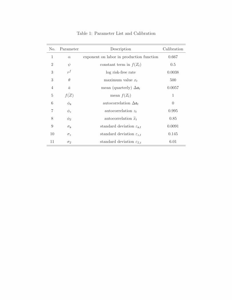
Table 1: Parameter List and Calibration

No. Parameter Description Calibration

1 α exponent on labor in production function 0.667

2 ψ constant term in f(Zt) 0.5

3 rf log risk-free rate 0.0038

3 θ maximum value xt 500

4 a mean (quarterly) ∆at 0.0057

5 ¯f(Z) mean f(Zt) 1

6 φa autocorrelation ∆at 0

7 φz autocorrelation zt 0.995

8 φx autocorrelation xt 0.85

9 σa standard deviation εa,t 0.0091

10 σz standard deviation εz,t 0.145

11 σx standard deviation εx,t 6.01

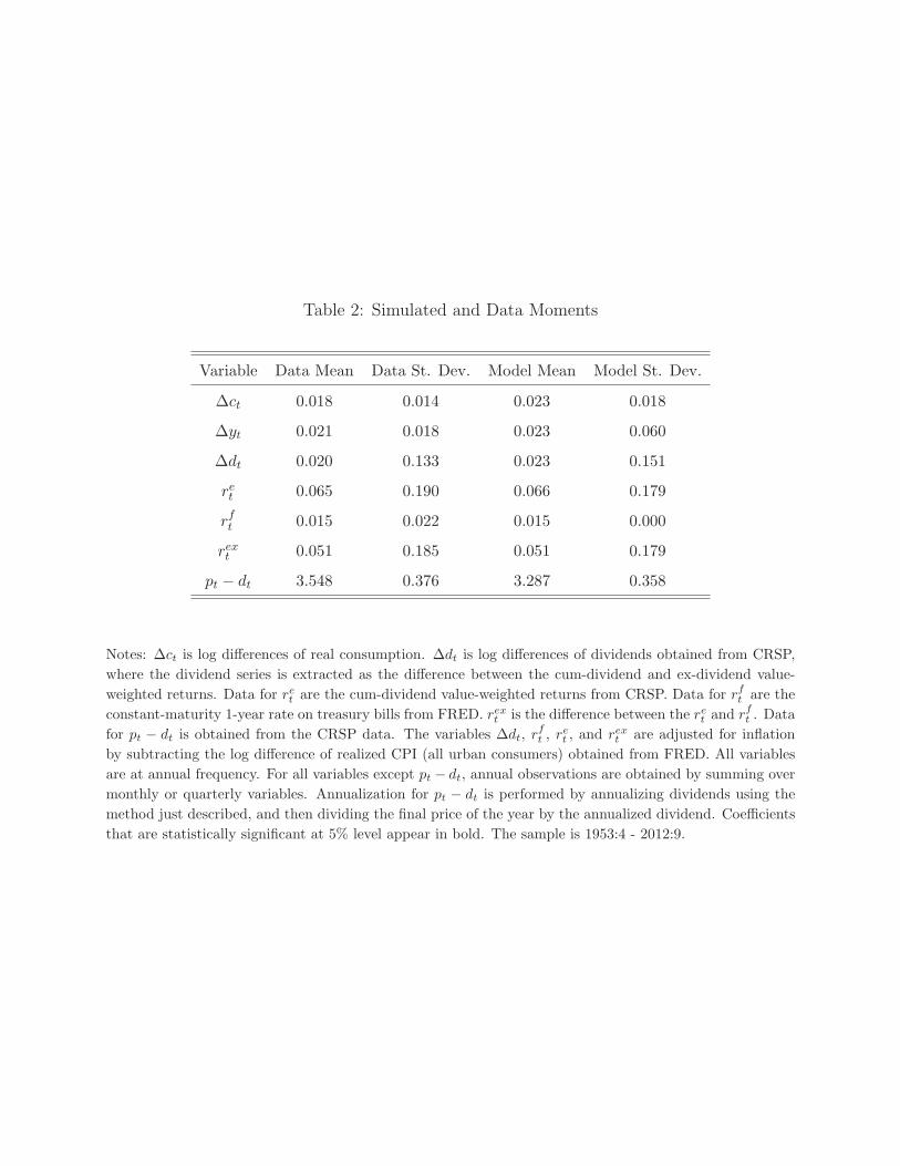
Table 2: Simulated and Data Moments

Variable Data Mean Data St. Dev. Model Mean Model St. Dev.

∆ct 0.018 0.014 0.023 0.018

∆yt 0.021 0.018 0.023 0.060

∆dt 0.020 0.133 0.023 0.151

ret 0.065 0.190 0.066 0.179

rft 0.015 0.022 0.015 0.000

rext 0.051 0.185 0.051 0.179

pt − dt 3.548 0.376 3.287 0.358

Notes: ∆ct is log differences of real consumption. ∆dt is log differences of dividends obtained from CRSP,

where the dividend series is extracted as the difference between the cum-dividend and ex-dividend value-

weighted returns. Data for ret are the cum-dividend value-weighted returns from CRSP. Data for rft are the

constant-maturity 1-year rate on treasury bills from FRED. rext is the difference between the ret and rft . Data

for pt − dt is obtained from the CRSP data. The variables ∆dt, rft , r

et , and rext are adjusted for inflation

by subtracting the log difference of realized CPI (all urban consumers) obtained from FRED. All variables

are at annual frequency. For all variables except pt − dt, annual observations are obtained by summing over

monthly or quarterly variables. Annualization for pt − dt is performed by annualizing dividends using the

method just described, and then dividing the final price of the year by the annualized dividend. Coefficients

that are statistically significant at 5% level appear in bold. The sample is 1953:4 - 2012:9.

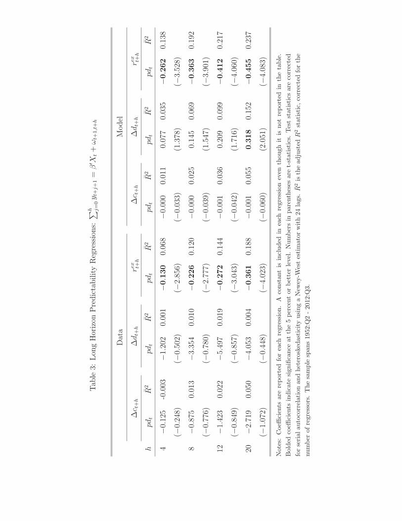
Tab

le3:

Lon

gHorizon

PredictabilityRegressions:

∑h j=0yt+

j+1=

β′X

t+ωt+

1,t+h

Data

Model

∆c t

+h

∆dt+

hrex

t+h

∆c t

+h

∆dt+

hrex

t+h

hpdt

R2

pdt

R2

pdt

R2

pdt

R2

pdt

R2

pdt

R2

4−0.125

-0.003

−1.202

0.001

−0.130

0.068

−0.000

0.011

0.077

0.035

−0.262

0.138

(−0.248)

(−0.502)

(−2.856)

(−0.033)

(1.378)

(−3.528)

8−0.875

0.013

−3.354

0.010

−0.226

0.120

−0.000

0.025

0.145

0.069

−0.363

0.192

(−0.776)

(−0.780)

(−2.777)

(−0.039)

(1.547)

(−3.901)

12−1.423

0.022

−5.497

0.019

−0.272

0.144

−0.001

0.036

0.209

0.099

−0.412

0.217

(−0.849)

(−0.857)

(−3.043)

(−0.042)

(1.716)

(−4.060)

20−2.719

0.050

−4.053

0.004

−0.361

0.188

−0.001

0.055

0.318

0.152

−0.455

0.237

(−1.072)

(−0.448)

(−4.023)

(−0.060)

(2.051)

(−4.083)

Notes:Coeffi

cients

arereportedforeach

regression

.A

constan

tis

included

ineach

regression

even

thou

ghit

isnot

reportedin

thetable.

Bolded

coeffi

cients

indicatesign

ificance

atthe5percentor

betterlevel.Numbersin

parentheses

aret-statistics.Teststatistics

arecorrected

forserial

autocorrelationandheteroskedasticity

usingaNew

ey-W

estestimator

with24

lags.R

2isthead

justed

R2statistic,

correctedforthe

number

ofregressors.Thesample

span

s19

52:Q

2-20

12:Q

3.

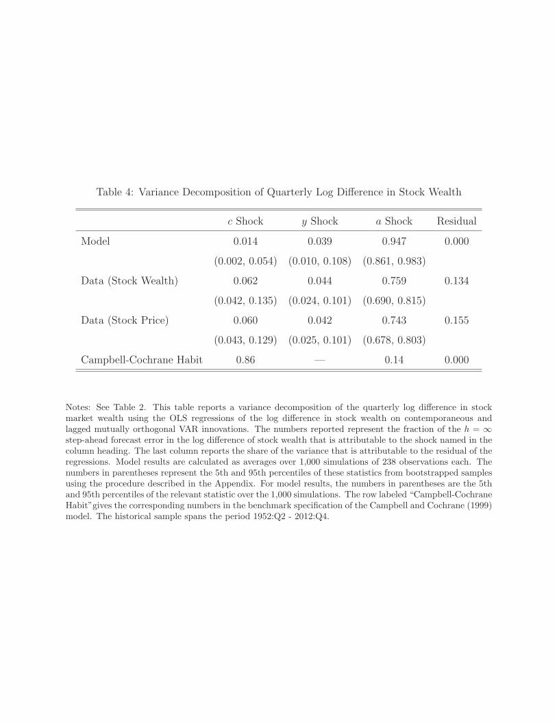
Table 4: Variance Decomposition of Quarterly Log Difference in Stock Wealth

c Shock y Shock a Shock Residual

Model 0.014 0.039 0.947 0.000

(0.002, 0.054) (0.010, 0.108) (0.861, 0.983)

Data (Stock Wealth) 0.062 0.044 0.759 0.134

(0.042, 0.135) (0.024, 0.101) (0.690, 0.815)

Data (Stock Price) 0.060 0.042 0.743 0.155

(0.043, 0.129) (0.025, 0.101) (0.678, 0.803)

Campbell-Cochrane Habit 0.86 — 0.14 0.000

Notes: See Table 2. This table reports a variance decomposition of the quarterly log difference in stockmarket wealth using the OLS regressions of the log difference in stock wealth on contemporaneous andlagged mutually orthogonal VAR innovations. The numbers reported represent the fraction of the h = ∞

step-ahead forecast error in the log difference of stock wealth that is attributable to the shock named in thecolumn heading. The last column reports the share of the variance that is attributable to the residual of theregressions. Model results are calculated as averages over 1,000 simulations of 238 observations each. Thenumbers in parentheses represent the 5th and 95th percentiles of these statistics from bootstrapped samplesusing the procedure described in the Appendix. For model results, the numbers in parentheses are the 5thand 95th percentiles of the relevant statistic over the 1,000 simulations. The row labeled “Campbell-CochraneHabit”gives the corresponding numbers in the benchmark specification of the Campbell and Cochrane (1999)model. The historical sample spans the period 1952:Q2 - 2012:Q4.

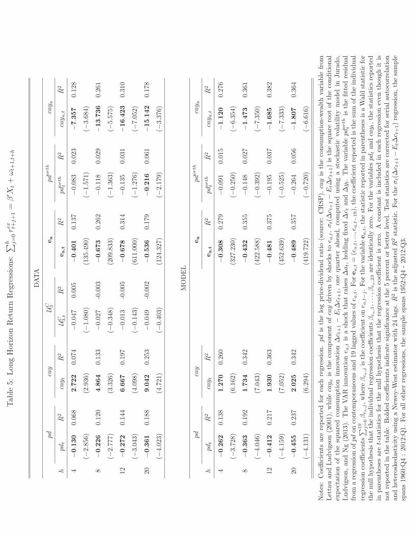
Tab

le5:

Lon

gHorizon

Return

Regressions:

∑h j=0rex

t+j+1=

β′X

t+ωt+

1,t+h

DATA

pd

cay

UC 3

ea

pdorth

cay a

hpdt

R2

cay t

R2

UC 3,t

R2

ea,t

R2

pdorth

tR

2cay a

,tR

2

4−0.130

0.06

82.722

0.07

4−0.04

70.00

5−0.401

0.13

7−0.08

30.02

3−7.357

0.12

8

(−2.85

6)(2.936)

(−1.08

0)(135.490

)(−

1.57

1)(−

3.68

4)

8−0.226

0.12

04.864

0.13

3−0.02

7-0.003

−0.673

0.26

2−0.11

80.02

9−13.736

0.26

1

(−2.77

7)(3.326

)(−

0.34

8)(209.833

)(−

1.36

3)(−

5.57

5)

12−0.272

0.14

46.667

0.19

7−0.01

3-0.005

−0.678

0.31

4−0.13

50.03

1−16.423

0.31

0

(−3.04

3)(4.098

)(−

0.14

3)(611.000

)(−

1.27

6)(−

7.05

2)

20−0.361

0.18

89.042

0.25

3−0.04

9-0.002

−0.536

0.17

9−0.216

0.06

1−15.142

0.17

8

(−4.02

3)(4.721

)(−

0.40

3)(124.327

)(−

2.17

9)(−

3.37

6)

MODEL

pd

cay

ea

pdorth

cay a

hpdt

R2

cay t

R2

ea,t

R2

pdorth

tR

2cay a

,tR

2

4−0.262

0.13

81.270

0.26

0−0.308

0.27

9−0.09

10.01

5−1.120

0.27

6

(−3.72

8)(6.162)

(327.230

)(−

0.25

0)(−

6.35

4)

8−0.363

0.19

21.734

0.34

2−0.432

0.35

5−0.14

80.02

7−1.473

0.36

1

(−4.04

6)(7.043)

(422.588

)(−

0.39

2)(−

7.35

0)

12−0.412

0.21

71.930

0.36

3−0.481

0.37

5−0.19

50.03

7−1.685

0.38

2

(−4.15

9)(7.052

)(452.639

)(−

0.52

5)(−

7.33

3)

20−0.455

0.23

72.025

0.34

2−0.489

0.35

7−0.26

40.05

6−1.807

0.36

4

(−4.131

)(6.294

)(419.722

)(−

0.72

0)(−

6.61

6)

Notes:Coeffi

cients

arereportedforeach

regression

.pdis

thelogprice-dividen

dratio(sou

rce:

CRSP).cayis

theconsumption

-wealthvariable

from

Lettauan

dLudvigson(2001

),whilecay a

isthecompon

entofc aydrivenbyshockstoe a

,t.σt(∆c t

+1−E

t∆c t

+1)is

thesquareroot

oftheconditional

expectation

ofthesquared

consumption

innovation∆c t

+1−E

t∆c t

+1,on

equarterah

ead,computedusingastochasticvo

latility

model

inJurado,

Ludvigson,an

dNg(201

3).TheVAR

innovatione a

,tis

ashock

that

raises

∆at,holdingfixed

∆c t

and∆y t.Thevariab

lepdorth

tis

thefitted

residual

from

aregression

ofpdon

contemporaneousan

d19

lagg

edvalues

ofe a

,t.For

ea,t=

(ea,t,...,e

a,t−19),thecoeffi

cientreportedisthesum

oftheindividual

regression

coeffi

cients

∑19

j=0βea,j,whereβea,jisthecoeffi

cienton

e a,t−j.For

thevariab

leea,t,thestatisticreportedin

parentheses

isaWaldstatisticfor

thenullhypothesisthat

theindividual

regression

coeffi

cientsβea,1,...,β

ea,23areidenticallyzero.For

thevariab

lespdtan

dcay t,thestatistics

reported

inparentheses

aret-statistics

forthenullhypothesis

that

theregression

coeffi

cientis

zero.A

constan

tis

included

ineach

regression

even

thoughit

isnot

reportedin

thetable.Bolded

coeffi

cients

indicate

sign

ificance

atthe5percentor

betterlevel.Teststatistics

arecorrectedforserial

autocorrelation

andheteroskedasticity

usingaNew

ey-W

estestimatorwith24

lags.R

2isthead

justedR

2statistic.

For

theσt(∆c t

+1−E

t∆c t

+1)regression

,thesample

s pan

s1960:Q

4:20

12:Q

1.For

allother

regression

s,thesample

span

s19

52:Q

4-20

12:Q

3.

Figure 1: Unconditional Distribution of Risk Aversion

0 50 100 150 200 250 300 350 400 450 5000

0.1

0.2

0.3

0.4

0.5

0.6

0.7

0.8

0.9

1

Risk Aversion, xt

Fre

quency

Mean

Median, Mode

Notes: Each bar represents the frequency with which the risk aversion variable xt falls in that specific bin.The median and mode are so close as to be indistinguishable on the plot.

Figure 2: Model-Based Responses: Primitive vs. VAR Shocks

5 10 15 20 0.01

0.005

0

0.005

0.01

Response!to!TFP!Shock

c

y

a

5 10 15 20 0.01

0.005

0

0.005

0.01

Response!to!dln!c!Shock

c

y

a

5 10 15 20 0.04

0.02

0

0.02

0.04

Response!to!Factor!Share!Shock

c

y

a

5 10 15 20 0.04

0.02

0

0.02

0.04

Response!to!dln!y!Shock

c

y

a

5 10 15 20

0.04

0.02

0

0.02

0.04

Response!to!Risk!Aversion!Shock

c

y

a

5 10 15 20

0.04

0.02

0

0.02

0.04

Response!to!dln!a!Shock

c

y

a

Notes: The left column plots the cummulated model impulse responses of the log differences of c, y, anda to the primitive shock named in the sub-graph title. The right column plots the cumulative impulseresponses implied by the model from a VAR in the log differences of c, y, and a to the orthogonalizedVAR shocks using data simulated from the model (right column). Impulse responses to primitive shocksare obtained by applying at t = 0 a one-standard deviation change in the direction that increases ∆at, andsimulating the model forward with all other shocks set to zero. Impulse responses to the VAR shocks areobtained by simulating the model over one very long sample (equal to 238,000 observations), estimating acointegrated VAR in the log differenced data, inverting to Wold representation and computing the responsesto orthogonalized c, y, and a shocks equal to one standard deviation changes in the direction that increases∆at with that ordering in the VAR. The size of the shocks are normalized so that the initial response of avariable to its own shock in the right panel is the same as the response of that variable to the correspondingprimitive shock in the left panel.

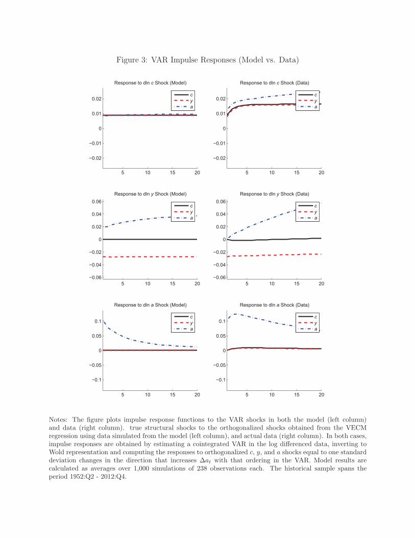
Figure 3: VAR Impulse Responses (Model vs. Data)

5 10 15 20

0.02

0.01

0

0.01

0.02

Response!to!dln!c!Shock!(Model)

c

y

a

5 10 15 20

0.02

0.01

0

0.01

0.02

Response!to!dln!c!Shock!(Data)

c

y

a

5 10 15 20

0.06

0.04

0.02

0

0.02

0.04

0.06

Response!to!dln!y!Shock!(Model)

c

y

a

5 10 15 20

0.06

0.04

0.02

0

0.02

0.04

0.06

Response!to!dln!y!Shock!(Data)

c

y

a

5 10 15 20

0.1

0.05

0

0.05

0.1

Response!to!dln!a!Shock!(Model)

c

y

a

5 10 15 20

0.1

0.05

0

0.05

0.1

Response!to!dln!a!Shock!(Data)

c

y

a

Notes: The figure plots impulse response functions to the VAR shocks in both the model (left column)and data (right column). true structural shocks to the orthogonalized shocks obtained from the VECMregression using data simulated from the model (left column), and actual data (right column). In both cases,impulse responses are obtained by estimating a cointegrated VAR in the log differenced data, inverting toWold representation and computing the responses to orthogonalized c, y, and a shocks equal to one standarddeviation changes in the direction that increases ∆at with that ordering in the VAR. Model results arecalculated as averages over 1,000 simulations of 238 observations each. The historical sample spans theperiod 1952:Q2 - 2012:Q4.

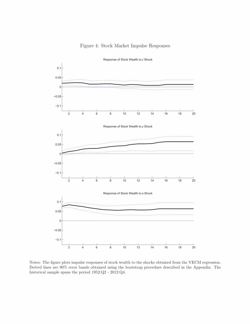
Figure 4: Stock Market Impulse Responses

2 4 6 8 10 12 14 16 18 20

0.1

0.05

0

0.05

0.1

Response!of!Stock!Wealth!to!c!Shock

2 4 6 8 10 12 14 16 18 20

0.1

0.05

0

0.05

0.1

Response!of!Stock!Wealth!to!y!Shock

2 4 6 8 10 12 14 16 18 20

0.1

0.05

0

0.05

0.1

Response!of!Stock!Wealth!to!a!Shock

Notes: The figure plots impulse responses of stock wealth to the shocks obtained from the VECM regression.Dotted lines are 90% error bands obtained using the bootstrap procedure described in the Appendix. Thehistorical sample spans the period 1952:Q2 - 2012:Q4.

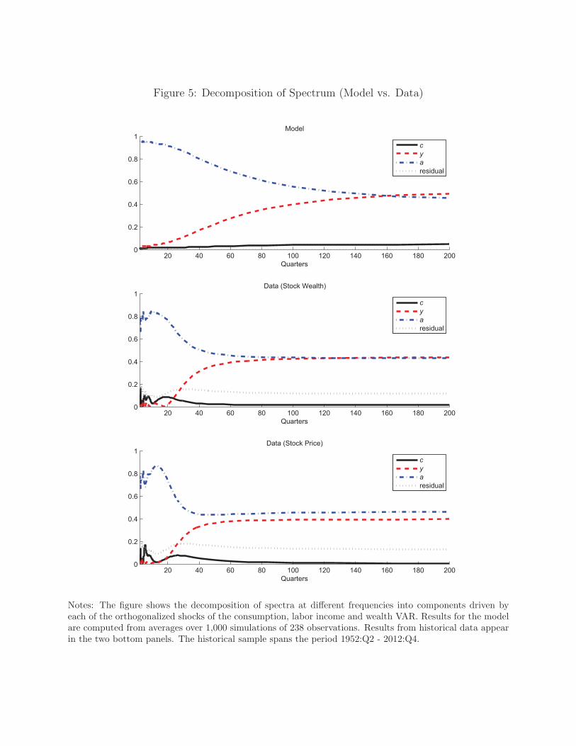
Figure 5: Decomposition of Spectrum (Model vs. Data)

20 40 60 80 100 120 140 160 180 2000

0.2

0.4

0.6

0.8

1

Quarters

Model

c

y

a

residual

20 40 60 80 100 120 140 160 180 2000

0.2

0.4

0.6

0.8

1

Quarters

Data!(Stock!Wealth)

c

y

a

residual

20 40 60 80 100 120 140 160 180 2000

0.2

0.4

0.6

0.8

1

Quarters

Data!(Stock!Price)

c

y

a

residual

Notes: The figure shows the decomposition of spectra at different frequencies into components driven byeach of the orthogonalized shocks of the consumption, labor income and wealth VAR. Results for the modelare computed from averages over 1,000 simulations of 238 observations. Results from historical data appearin the two bottom panels. The historical sample spans the period 1952:Q2 - 2012:Q4.

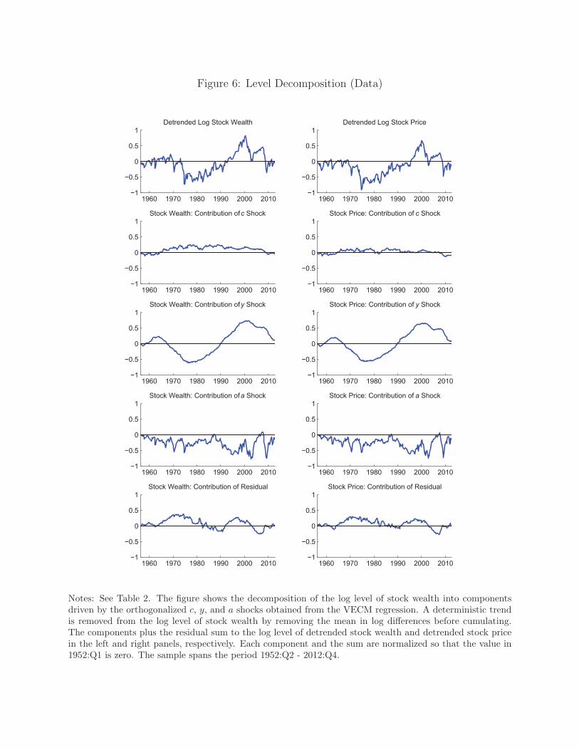
Figure 6: Level Decomposition (Data)

1960 1970 1980 1990 2000 2010 1

0.5

0

0.5

1

Detrended!Log!Stock!Wealth

1960 1970 1980 1990 2000 2010 1

0.5

0

0.5

1

Stock!Wealth:!Contribution!of!c!Shock

1960 1970 1980 1990 2000 2010 1

0.5

0

0.5

1

Stock!Wealth:!Contribution!of!y!Shock

1960 1970 1980 1990 2000 2010 1

0.5

0

0.5

1

Stock!Wealth:!Contribution!of!a!Shock

1960 1970 1980 1990 2000 2010 1

0.5

0

0.5

1

Stock!Wealth:!Contribution!of!Residual

1960 1970 1980 1990 2000 2010 1

0.5

0

0.5

1

Detrended!Log!Stock!Price

1960 1970 1980 1990 2000 2010 1

0.5

0

0.5

1

Stock!Price:!Contribution!of!c!Shock

1960 1970 1980 1990 2000 2010 1

0.5

0

0.5

1

Stock!Price:!Contribution!of!y!Shock

1960 1970 1980 1990 2000 2010 1

0.5

0

0.5

1

Stock!Price:!Contribution!of!a!Shock

1960 1970 1980 1990 2000 2010 1

0.5

0

0.5

1

Stock!Price:!Contribution!of!Residual

Notes: See Table 2. The figure shows the decomposition of the log level of stock wealth into componentsdriven by the orthogonalized c, y, and a shocks obtained from the VECM regression. A deterministic trendis removed from the log level of stock wealth by removing the mean in log differences before cumulating.The components plus the residual sum to the log level of detrended stock wealth and detrended stock pricein the left and right panels, respectively. Each component and the sum are normalized so that the value in1952:Q1 is zero. The sample spans the period 1952:Q2 - 2012:Q4.

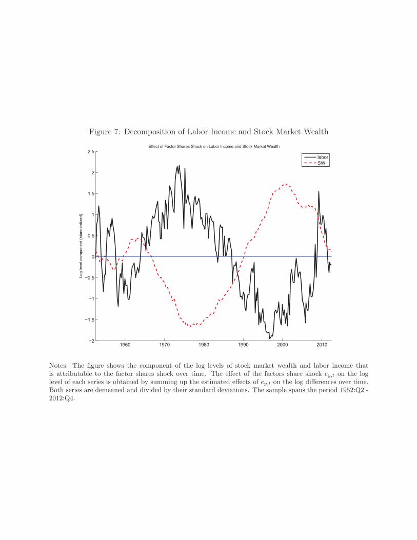
Figure 7: Decomposition of Labor Income and Stock Market Wealth

1960 1970 1980 1990 2000 2010 2

1.5

1

0.5

0

0.5

1

1.5

2

2.5

Log!level!component!(standardized)

Effect!of!Factor!Shares!Shock!on!Labor!Income!and!Stock!Market!Wealth

labor

SW

Notes: The figure shows the component of the log levels of stock market wealth and labor income thatis attributable to the factor shares shock over time. The effect of the factors share shock ey,t on the loglevel of each series is obtained by summing up the estimated effects of ey,t on the log differences over time.Both series are demeaned and divided by their standard deviations. The sample spans the period 1952:Q2 -2012:Q4.

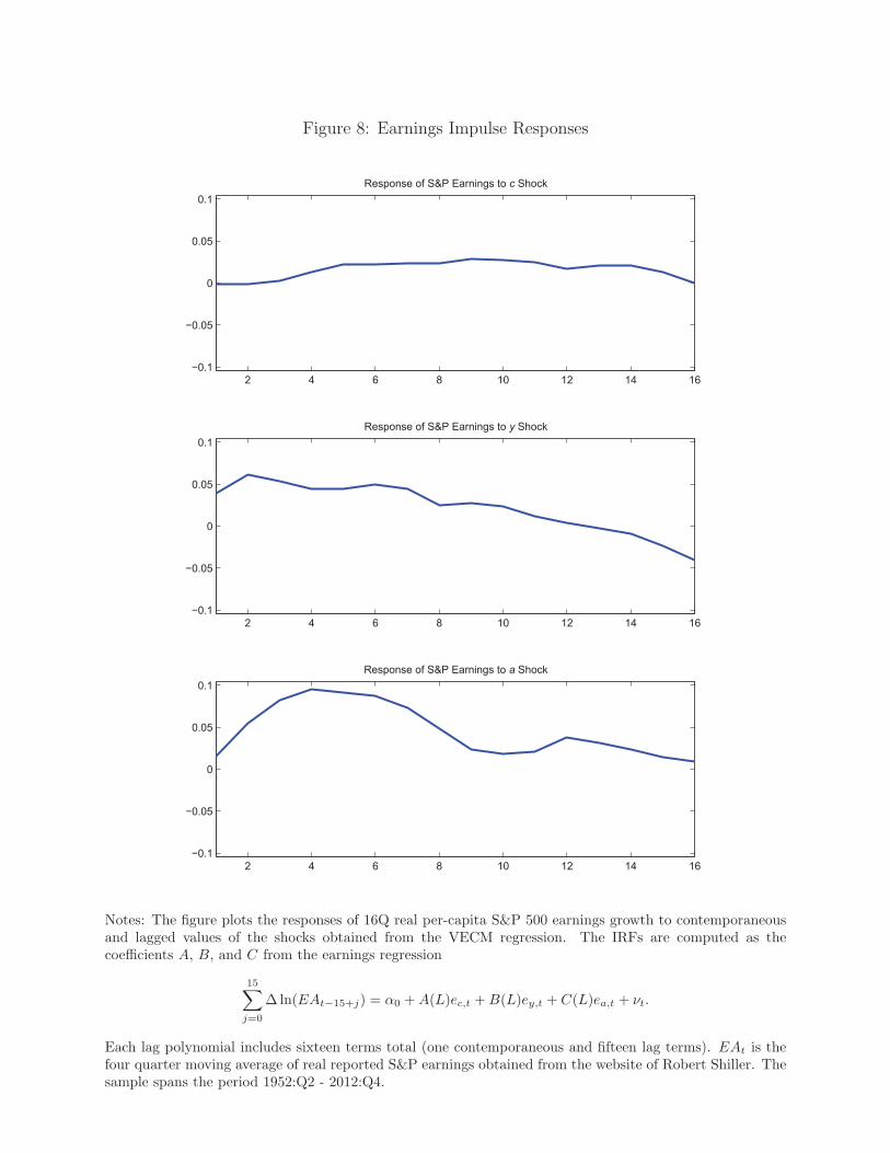
Figure 8: Earnings Impulse Responses

2 4 6 8 10 12 14 16

0.1

0.05

0

0.05

0.1

Response!of!S&P!Earnings!to!c!Shock

2 4 6 8 10 12 14 16

0.1

0.05

0

0.05

0.1

Response!of!S&P!Earnings!to!y!Shock

2 4 6 8 10 12 14 16

0.1

0.05

0

0.05

0.1

Response!of!S&P!Earnings!to!a!Shock

Notes: The figure plots the responses of 16Q real per-capita S&P 500 earnings growth to contemporaneousand lagged values of the shocks obtained from the VECM regression. The IRFs are computed as thecoefficients A, B, and C from the earnings regression

15∑

j=0

∆ ln(EAt−15+j) = α0 +A(L)ec,t +B(L)ey,t + C(L)ea,t + νt.

Each lag polynomial includes sixteen terms total (one contemporaneous and fifteen lag terms). EAt is thefour quarter moving average of real reported S&P earnings obtained from the website of Robert Shiller. Thesample spans the period 1952:Q2 - 2012:Q4.

Figure 9: Gini Coefficient and Cumulated ey Shock

1980 1985 1990 1995 2000 2005 2

1.5

1

0.5

0

0.5

1

1.5

2

Consumption!Gini!(Data)

Cumulated y!Shock

Implied!Consumption!Gini!(Model)

Notes: The consumption Gini (data) series is the Gini coefficient of inequality for nondurable consumption(source: Heathcote, Perri and Violante (2010)). The cumulated y shock series is the running total of allthe ey shocks to date:

∑t

j=1ej . The implied consumption Gini (model) series uses the model to calculate

the implied Gini coefficient for consumption based on the observed sequence of y shocks (see appendix fordetails). All series are presented at annual frequency. For the cumulated y shock and model-implied Giniseries, annual observations are averages over the calendar year. All three series are normalized to have zeromean and unit standard deviation in the sample.

A Additional Figures

Figure A.1: Consumption Shocks and TFP

Notes: The TFP shock series is differenced Business Sector TFP (source: Fernald). The consumption shockseries is taken from the VECM. The sample spans the period 1947:Q2 - 2013:Q3.

Figure A.2: 16Q Moving Averages of Labor Share and TFP

1960 1970 1980 1990 2000 2010 3

2

1

0

1

2

3

16Q!Moving!Average!of!dTFP,!dLS

Quarterly!correlation!of!dTFP,!dLS!=! 0.43

dTFP

dLS

Notes: The series are 16Q moving averages of each series in log differences. TFP is Business Sector TFP(source: Fernald). LS is Nonfarm Business Sector Labor Share (source: BLS). The sample spans the period1947:Q2 - 2013:Q3.

Figure A.3: VAR Impulse Responses with Error Bands

5 10 15 20

0.03

0.02

0.01

0

0.01

0.02

0.03

c!Shock

c

5 10 15 20

0.03

0.02

0.01

0

0.01

0.02

0.03

c!Shock

y

5 10 15 20

0.03

0.02

0.01

0

0.01

0.02

0.03

c!Shock

a

5 10 15 20

0.03

0.02

0.01

0

0.01

0.02

0.03

y!Shock

c

5 10 15 20

0.03

0.02

0.01

0

0.01

0.02

0.03

y!Shock

y

5 10 15 20

0.03

0.02

0.01

0

0.01

0.02

0.03

y!Shock

a

5 10 15 20

0.03

0.02

0.01

0

0.01

0.02

0.03

a!Shock

c

5 10 15 20

0.03

0.02

0.01

0

0.01

0.02

0.03

a!Shock

y

5 10 15 20

0.03

0.02

0.01

0

0.01

0.02

0.03

a!Shock

a

Notes: The figure plots impulse response functions to the VAR shocks obtained from the VECM regressionusing data. Impulse responses are obtained by estimating a cointegrated VAR, inverting to Wold represen-tation and computing the responses to orthogonalized c, y, and a shocks with that ordering in the VAR. Thedotted lines are 90% error bands obtained using the bootstrap procedure described in the Appendix. Thehistorical sample spans the period 1952:Q2 - 2012:Q4.

Figure A.4: Model Gini Coefficient

0 0.1 0.2 0.3 0.4 0.5 0.6 0.7 0.8 0.9 10

0.1

0.2

0.3

0.4

0.5

0.6

0.7

0.8

0.9

1

Consumption!Quantile

Consumption!Share

A

B

(1 � q, α f (z))

Notes: This diagram plots the distribution of consumption in the model. q is the proportion of shareholders.The Gini coefficient of consumption is defined by G = A/(A + B), where A and B are the areas of therelevant regions.