Organizational cultures of corruption∗

Patrick Schneider and Gautam Bose †

September 7, 2015

Abstract

Systematic differences in the incidence of corruption between countries can be ex-plained by models of coordination failure that suggest that corruption can only bereduced by a “big push” across an entire economy. However, there is significant ev-idence that corruption is often sustained as an organizational culture, and can becombated with targeted effort in individual organizations one at a time. In this paperwe propose a model that reconciles these two theories of corruption.

We explore a model of corruption with two principal elements. First, agents suffera moral cost if their corruption behavior diverges from the level they perceive to be thesocial norm; second, the perception of the norm is imperfect; it gives more weight tothe behavior of colleagues with whom the agent interacts regularly. This leads to thepossibility that different organizations within the same country may stabilize at widelydifferent levels of corruption. Further, the level of corruption in an organization ispersistent, implying that some organizations may have established internal ‘cultures’ ofcorruption. The organizational foci are determined primarily by the opportunities and(moral) costs of corruption. Depending on the values of these parameters the degreeof corruption across departments may be relatively uniform or widely dispersed.

These results also explain another surprising empirical observation: that in differentcountries similar government departments such as tax and education rank very differ-ently relative to each other in the extent to which they are corrupt. This is difficultto explain in incentive-based models if similar departments face similar incentives indifferent countries.

Keywords: corruption, cognitive dissonance, perception, social norms.

∗This paper is partly based on Schneider’s undergraduate honors thesis submitted to UNSW. We areindebted to Zhanar Akhmetova, Ariel Ben Yishay, Richard Holden, Hodaka Morita and Alberto Motta forcomments at various stages of this project. Correspondence to g.bose@unsw.edu.au.†University of New South Wales.

1. Introduction

Levels of corruption differ significantly between countries.1 Coordination models providea standard way to explain such differences and suggest that anti-corruption efforts shouldinvolve ‘big-push’ policies that ensure all agents shift expectations and behavior simultane-ously to the desirable equilibrium (see, e.g., Andvig and Moene (1990) and the referencestherein, Murphy et al. (1993); Nabin and Bose (2008)). The persistence and pervasiveness ofcorruption in some countries coupled with its systematic absence in others strongly supportthe insights of coordination models.

Corrupt practices also vary substantially across different regions or organizations withinindividual countries. This within-country variation can be explained at the level of organi-zations, with differences in corruption caused by differing incentives or management regimesand exacerbated by selection.2 These lower level models suggest corruption can be cleaned upwithin organizations by altering the incentive structures that agents face. There are exam-ples in the literature of successful anti-corruption efforts targeting individual organizations,for example in Klitgaard (1988).

There is a disjuncture in the insights that these approaches provide. The latter suggeststhat it is feasible to clean up organizations with targeted policies. The former approach, onthe other hand, suggests that this should not be possible—only an economy-wide effort willwork. However, while they produce conflicting policy recommendations, both approacheshave empirical support.

In this paper we propose a simple model of coordination on social norms (Rabin, 1994;Fischer and Huddart, 2008) to reconcile the two approaches. An agent in our model chooseshow much to exploit opportunities for corruption but incurs a cost in doing so. The mag-nitude of this cost depends on his individual perception of the social norm regarding ‘ac-ceptable’ corruption, which is an aggregation of the positions held by his peers within thesame organization as well as agents across the society. It is crucial to our model that theagent’s perception is more heavily influenced by the stances of his immediate peers thanby those outside his organization. In equilibrium, each organization coordinates on a localnorm which we term its ‘organizational focus’. Different organizations may coordinate onwidely different foci even when agents are homogeneous, self-selection is absent, and thereare no differences in incentives. This result is consistent with the empirical observation thatcorruption levels between organizations vary more than differences in incentives can explain(Schneider, 2011).

We define the ‘social norm’ as the employment-weighted average behavior across all or-ganizations. The individual agent’s perception of the social norm, however, is imperfect; it

1Evident in casual observation as well as increasing numbers of corruption measures such as TransparencyInternational’s indices.

2An important institutionalized selection mechanism that has been long known in the Indian context isthe sale of “lucrative” administrative positions based on the bribe-income that an incumbent is able to earnduring the tenure of his posting. See Wade (1982, especially pp. 302-307) for an early and detailed study,and also Wade (1985).

1

accords positive weight to the behavior of his organizational colleagues (the local norm) aswell as the true social norm. When his perception is limited only to the local norm, the cul-ture in each organization is independent of the rest of the economy. Similarly, when agentsaccurately perceive the social norm, all organizations in the economy share a homogeneousculture. However, when agents are influenced by both their local and the global norm, differ-ences between organizations can be sustained in equilibrium. We identify conditions underwhich the equilibrium distribution of organizational foci in an economy is non-degenerate.

An equilibrium in our model is a state in which each agent in each organization optimallyresponds to his perceived social norm, and these responses give rise to the correspondingorganizational foci. Note that it is not necessary that all organizations have the same focusin equilibrium. There may be multiple sustainable foci within an equilibrium. Further notethat multiple equilibria can obtain, each with its own distribution of organizational foci,depending on the extant global norm. For example, for a given global norm, there maybe an equilibrium in which some organizations focus on high and some on low levels ofcorruption, and another equilibrium in which all organizations focus on the same level ofcorruption. The requisite global norm is maintained in equilibrium if appropriate proportionsof organizations occupy the admissible organizational foci.

Even with homogeneous agents and exogenously determined incentives, our model leadsto a richer set of policy possibilities than pure coordination models. Since organizational fociare determined in part by endogenously generated norms, the extent of corruption withinan organization can be successfully reduced by a targeted initiative even without changes inthe rest of the economy. However, the extent of corruption within the organization also doescontribute to the social average. As a result, changes in one organization will flow throughto others, at least in small measure. We know that such targeted efforts do yield results,as documented, for example, by Klitgaard (1988) in the case of the Hong Kong police forceand of the Philippines income tax department. An effort to rid a corrupt economy of themalady could thus target organizations sequentially, or it could target them simultaneouslyas in a “big push”. If a sequential strategy is followed, then the most efficient sequencingis to first target the organizations that will have the largest impact on the social norm perunit of cost.

The mechanism we employ utilizes a social dynamic that is well-established in social psy-chology and other related literatures. People experience costs in terms of social opprobriumor negative feelings when they do something perceived to be ‘bad’ (Coleman, 1990; Basu,2000; Akerlof, 1976; Elster, 1989). But these costs depend on the attitudes of those aroundthem because their peers help them get a view of what is normal (Bardhan, 1997; Sardan,1999; Arendt, 1977), help them develop rationalizations to avoid classifying the activity asbad at all, thus avoiding the cost (Cressey, 1971; Laub, 2006), or involve them in a web ofcomplicity so as to nullify objection (Ashforth and Anand, 2003).3

3Rasmusen (1996) shows that when the crime rate is high workers with prior criminal convictions face lesssocial stigma (in terms of lower wages). However, the result is driven by adverse selection rather than peereffects: criminals are less productive than non-criminals and in high-crime environments there is a higherproportion of unconvicted criminals, bringing the expected productivity of this population closer to that of

2

As with the rose, our mechanism by any other name would work as well. Our analyticalresults derive from two critical assumptions: first, that the individual’s perception of thesocial norm is a convex combination of the true social norm and the local norm, and secondly,that there is a cost when the individual’s behavior deviates from this perceived norm. Wemotivate our model with reference to culture and norm-conforming preferences because webelieve this reflects actual behavior. However, the model is capable of other interpretations;for example, the probability of detection, censure and punishment for corrupt acts (as wellas praise or reward for eschewing them) may depend on the extent to which an individual’spractice deviates from those of his organizational colleagues.

We interpret culture as the modes of behavior and language employed by groups of closelyinteracting people. There are differences in corruption and attitudes toward it that cannotreasonably be explained with reference to normal incentives. For example, four of the lasteight governors of Illinois4 have criminal convictions, whereas none in Indiana do. Certainlythere are differences in the neighboring states but the contrast is stark, and there is noreason to think the incentives are that different. Similarly, in their study on shirking inbranches of the same corporations located in different regions of Italy, Ichino and Maggi(2000) find systematic differences between northern and southern branches. Further, theyfind that employees that relocate from one region to the other tend to change their behaviorto conform to the local norm.

In the context of comparative corruption between countries, Schneider (2011, Chapter7), finds unexplained variation in corruption levels between government departments withincountries. Not surprisingly, corruption is higher across the board in some countries thanin others, and some departments or authorities are on average more corrupt than otherdepartments or authorities once country effects are accounted for. However, the latter effectis significantly less systematic than one would expect on the basis of a simple, incentive-driven model. There is a sufficiently large number of instances in which department A issignificantly more corrupt than department B in some countries, while the opposite is trueelsewhere. An explanation for this variation is that individual departments idiosyncraticallydevelop distinct cultures of corruption, which is the way we prefer to interpret our results.

Past papers have employed aspects of these dynamics to model corrupt or otherwise ‘bad’behavior. The cost of immorality, for example, is introduced exogenously by Blackburn et al.(2006) and Bose and Gangopadhyay (2009) by incorporating corruptible and incorruptibleagents, and by Klitgaard (1988) who introduces agents who suffer a fixed moral cost for theiractions. Alternately, cognitive dissonance and rationalization has been invoked by Akerlofand Dickens (1982) and Rabin (1994) to show how the interaction between one’s behavior,one’s own moral line and the behavior of peers can interact to support damaging behavior.

In Glaeser et al. (1996), agents choose whether or not to commit crimes. Some agentsare influenced by their neighbors’ choices while other agents are not. The latter type induceboundaries that contain the diffusion of influence, forming distinct neighborhoods across

convicted criminals.4Rod Blagojevich (2003-09), George H. Ryan (1999-2003), Dan Walker (1973-77) and Otto Kerner, Jr

(1962-68).

3

which crime rates can vary significantly. Our model is somewhat similar, but instead ofdifferent types of agents we rely on organizational boundaries and perception to generatelocal differences. Fischer and Huddart (2008) develop a model that brings these issuestogether in a fashion similar to ours—agents choose the level at which they undertake anaction and suffer a cost that depends on the (endogenous) social norms among their peers.They find that, within this structure, norms influence the effectiveness of other incentives,determine the ideal way to group agents and also guide self-selection. These two papers comethe closest to fully endogenizing social norms, though they rely on heterogeneous agents toproduce the key results.

Our model builds on this literature. We introduce locally biased perception to endogenizesocial norms. This modification allows us to construct a particularly simple model thatgenerates novel insights. The model focuses solely on a ‘bad’ action and an associatedinternalized cost that depends on the choices of others. Structured thus, it could applyequally to different settings (e.g. government or private) and to applications other thancorruption. The coordination that the model produces follows naturally from its structure.Its utility is in its ability to produce, in an extremely simple framework, a variety of observedbehaviors by homogeneous agents that coexist in equilibrium.

We do not invoke heterogeneity between agents or between the incentives for corruptionin different organizations. The heuristic discussion of the general model in Section 2 indi-cates that a large number of foci are possible within a single equilibrium depending on howperceptions are formed. In the closed-form model of Sections 3 and 4 we use a strictly con-vex moral cost function and a (weakly) concave utility function, and hence obtain equilibriawith at most two distinct organizational foci. It will be readily obvious that if agents wereheterogeneous, or they were to self-select into organizations based on their own predisposi-tions towards being corrupt, this would strengthen our results and produce a richer spreadof organizational foci without contradicting our policy conclusions.

Our emphasis is on the role of social norms in determining corruption, so for clarity weabstract from the possibility that corrupt acts may attract a probabilistic penalty. Alter-natively, the cost in the model may be interpreted as already incorporating the expectedexogenous penalty.

Section 2 describes the model. Section 3 discusses how each organization’s focus isdetermined. Section 4 establishes the equilibria for the whole economy. Section 5 discussesthe policy implications and concludes the paper.

2. The model

2.1. Organizations, agents and perceptions

The economy consists of J departments, indexed by j. Department j employs a numberNj of officials indexed by ij. All officials earn a common wage which we normalize to zero.Each official also faces opportunities for corruption from which he can earn a maximumadditional income bij. The extent to which he actually indulges in these opportunities

4

ψij ∈ [0, 1] is his choice. His income is then ψijbij, from which he derives a benefit

U(ψijbij) where U ′ > 0 and U ′′ ≤ 0.

While the official can choose his behavior, it is costly to act in a way that deviates fromwhat he perceives to be the social norm φ (to be explained below). If the official wishes tomaintain behavior ψ 6= φ, he incurs a (psychological or moral) cost:

C(ψ, φ), where Cψ > 0, Cφ < 0, Cψψ > 0 and Cψφ < 0.

The cost is increasing and convex in ψ, and decreasing in the perceived level of corruption inthe society. Further, the marginal cost of a small increase in personal corruption is smaller,ceteris paribus, when the perceived social corruption is larger.

The official does not perfectly observe the norm of his broader society, θ ∈ [0, 1]. Instead,he forms a perception based on the average of the behavior of those in his department,

ψj =

∑i ψijNj

(1)

and the society-wide norm θ.We will discuss the genesis of θ later; for the moment we assumeit to be exogenous. So the officials in department j perceive the social norm to be5

φj = Φ(ψj, θ), min{ψj, θ} ≤ Φ(ψj, θ) ≤ max{ψj, θ}, 0 < Φψ,Φθ < 1. (2)

Each official’s payoff is the sum of the utility from his corruption income and his moralcost. The official chooses ψij to maximize this objective function, with his perception of thesocial norm φj taken as given. Thus his optimization problem is:

maxψij

Vij(ψij, φj) = U(ψijbij)− C(ψij, φj) (3)

It follows that ψij is a function of bij and φj. The organization’s average behavior is thenΨj(φj, θ) as in (1), where the individual behavior choices ψij solve (3).

It is intuitively obvious that, for given θ, an average behavior ψj can persist in departmentj only if it gives rise to a perception φj which in turn leads its officials to optimally chooseactions that average to ψj. Further, this average behavior will be stable against smallperturbations in perceptions or actions if, for φ close to φj, the averaged optimal responseto φ leads perceptions to be revised in the direction of φj. Formally,

5In the body of the paper we assume that all officers perceive exactly the average behavior in theirdepartment and in the wider society, and compute their perceptions with a bias towards the departmentalaverage. In an appendix, we discuss how the results are modified if we assume a more realistic process whereeach officer forms his perception based on a number of observations of actions by other agents, with a biastowards his departmental colleagues.

5

Definition 1 (Organizational focus) For a given θ we define an organization’s focus asa ψj with an associated φj such that

(ψj, φj) = (Ψj(φj, θ), Φ(ψj, θ)) (4)

Further, a focus is stable if there is a neighborhood N(φj) of φj such that, for φ ∈ N(φj)⋂

[0, 1],Ψ(φ, θ) ∈ (φ, φj].

In other words, at a stable organizational focus, ψj and φj are consistent with eachother via the optimization behavior of the officials, and a small perturbation in actions orperceptions from (ψj, φj) is self-correcting.6

An equilibrium for the economy is a set of stable organizational foci ψj, j = 1, ..., J anda social norm θ, such that ψj is a focus for j given θ, and θ is the economy-wide averagelevel of corruption that results from the foci ψj, j = 1, ..., J . We assume

θ =

∑j[Njψj]∑j Nj

, (5)

i.e., it is the average of the departmental corruption levels weighted by their populationweights. Thus an equilibrium is a set of organizational foci that are mutually consistent.

At an organizational focus, by (2) all officials within department j have the same per-ception φj, since φj is determined by the economy-wide variable θ and the department-levelvariable ψj. Thus the moral stances of officials within a department will cluster around thecommon mean ψj, deviating from the mean according to the extent to which a particularofficial faces corruption opportunities greater or less than the average.

To simplify the exposition and focus on the essential intuition of the model, we willhenceforth assume that all officials in all departments face the same corruption opportunities,i.e.,

bij = b ∀i, j.

It follows that, within a given department j, all officials will choose the same level of cor-ruption,

ψij = Ψ(φj) = arg maxψij

U(ψijb)− C(ψij, φj) (6)

which is also the average level of corruption in the department, i.e.,

ψj ≡ Ψ(φj) (7)

Allowing the bijs to vary across i and j would yield greater variations in corruption withinand between departments, enhancing our results. An examination of (3) and (6) will showthat nothing further is lost from this simplification.

6A focus is a dynamically stable partial equilibrium for the department. To avoid confusion we reservethe term “equilibrium” to refer to a general equilibrium for the economy.

6

2.2. Intuition

For given θ the focus of a department j is determined by the three equations, (2), (6)and (7). Note that (6) is in fact a set of Nj identical equations determining the corruptionlevels of the individual officials. By virtue of (7), this further reduces to two equations inthe two variables ψj and φj.

From (2) it follows that Φ(ψj, θ) lies between ψj and θ, has a positive slope less thanunity with respect to ψj, and intersects the diagonal of the unit square at ψj = θ.

The variable ψj is constrained to lie in the unit interval. At an interior optimum, theindividual official’s choice ψij satisfies:

bU ′(ψijb) = C ′(ψij) (8)

Extremal choices must satisfy corresponding inequality conditions. By (7) it follows that ψjsatisfies the same condition.

When the solution to (6) is interior, (8) is satisfied with equality and we can derive theslope of ψj with respect to φ as:

∂Ψ(φ)

∂φ=

Cψφb2U ′′ − Cψψ

(9)

Given the assumptions on the partials of the cost function and the utility function, it followsthat Ψ(φ) is positively sloped. To further pin down the shape of the function Ψ(φ) requiresassumptions about the third partials and cross-partials of the utility and cost functions. Wewill eschew this; instead in the closed-form model of the next section we show that thereexist reasonable conditions under which it has a shape that yields satisfactory results.

Organizational foci

Figure 2.2 draws two representations of the graphs of Ψ(φ) and Φ(ψ, θ), with φ on thehorizontal axis.

If (φj, ψj) lies above the graph of Ψ(φ), then the individual choices leading to ψj aretoo high for optimum given the perception. This leads officials to reduce their corruptionchoices, hence (φj, ψj) must adjust vertically downwards. conversely if (φj, ψj) lies below thecurve, individual actions will adjust ψj upwards.

We draw Φ(ψj, θ) it with φ on the horizontal axis so it has a positive slope steeper thanunity. Note that if (φj, ψj) is to the left of this curve, then the perception φj is too lowgiven ψj and θ, so the adjustment in perception moves (φj, ψj) horizontally to the right.The reverse is true if (φj, ψj) is to the right of the curve.

A configuration (ψ, φ) is a potential organizational focus if the graphs of Ψ(.) and Φ(., θ)intersect at (ψ, φ), or if (8) is satisfied with inequalities corresponding to corner solutions.However, only some of these solutions are stable (se Definition 1), as discussed below, andhence candidates for continuing organizational cultures.

7

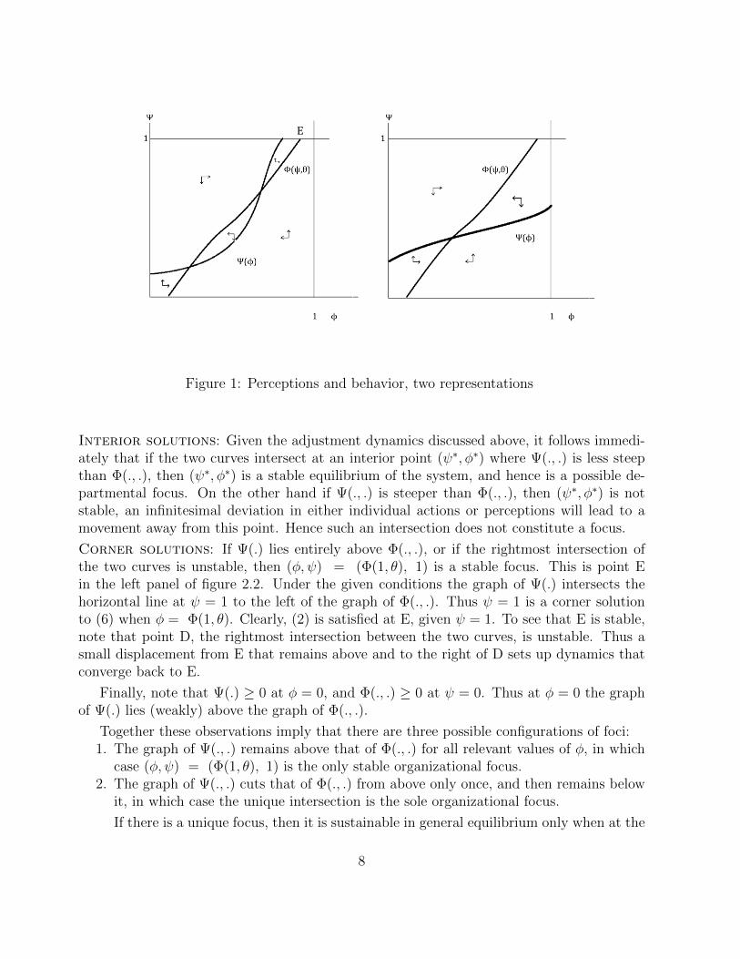
             E            

Figure 1: Perceptions and behavior, two representations

Interior solutions: Given the adjustment dynamics discussed above, it follows immedi-ately that if the two curves intersect at an interior point (ψ∗, φ∗) where Ψ(., .) is less steepthan Φ(., .), then (ψ∗, φ∗) is a stable equilibrium of the system, and hence is a possible de-partmental focus. On the other hand if Ψ(., .) is steeper than Φ(., .), then (ψ∗, φ∗) is notstable, an infinitesimal deviation in either individual actions or perceptions will lead to amovement away from this point. Hence such an intersection does not constitute a focus.

Corner solutions: If Ψ(.) lies entirely above Φ(., .), or if the rightmost intersection ofthe two curves is unstable, then (φ, ψ) = (Φ(1, θ), 1) is a stable focus. This is point Ein the left panel of figure 2.2. Under the given conditions the graph of Ψ(.) intersects thehorizontal line at ψ = 1 to the left of the graph of Φ(., .). Thus ψ = 1 is a corner solutionto (6) when φ = Φ(1, θ). Clearly, (2) is satisfied at E, given ψ = 1. To see that E is stable,note that point D, the rightmost intersection between the two curves, is unstable. Thus asmall displacement from E that remains above and to the right of D sets up dynamics thatconverge back to E.

Finally, note that Ψ(.) ≥ 0 at φ = 0, and Φ(., .) ≥ 0 at ψ = 0. Thus at φ = 0 the graphof Ψ(.) lies (weakly) above the graph of Φ(., .).

Together these observations imply that there are three possible configurations of foci:1. The graph of Ψ(., .) remains above that of Φ(., .) for all relevant values of φ, in which

case (φ, ψ) = (Φ(1, θ), 1) is the only stable organizational focus.2. The graph of Ψ(., .) cuts that of Φ(., .) from above only once, and then remains below

it, in which case the unique intersection is the sole organizational focus.

If there is a unique focus, then it is sustainable in general equilibrium only when at the

8

intersection ψ = φ = θ. Note that all organizations would then have this same focus,in turn justifying θ = ψ. If the unique intersection is interior, then all organizationschoose the same ψj, and hence we must again have ψj = φj = θ for all j. To determinethe full equilibrium for the economy requires us to endogenize θ, which is addressed inSection 4.The unique focus may be at (0, 0) if θ = 0. This is an equilibrium with no corruptionin the economy. Alternatively the unique focus may be at (Φ(1, θ), 1). Then allorganizations must choose ψ = 1, implying θ = 1, so the economy is completelycorrupt. In turn this implies φj = 1 for all j.

3. The graphs may intersect more than once in the interior. The leftmost intersection mustproduce a stable focus (since at φ = 0 the graph of Ψ(.) lies (weakly) above the graphof Φ(., .)). The next intersection must therefore be unstable (the graphs intersect inthe “wrong” direction), and every odd-numbered intersection must be stable. Finally,if the rightmost intersection is unstable then there is an extreme focus at (Φ(1, θ), 1).

When there are multiple foci, θ is a weighted average of the corruption levels chosen byorganizations that locate at the various foci. It is important to emphasize that the multiplefoci still constitute a single equilibrium for the economy, in which different organizationslocate at different levels of corruption.

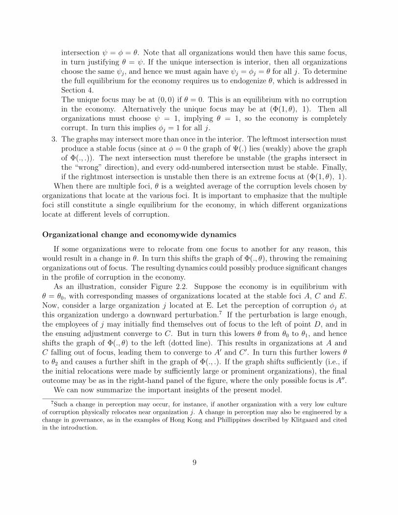
Organizational change and economywide dynamics

If some organizations were to relocate from one focus to another for any reason, thiswould result in a change in θ. In turn this shifts the graph of Φ(., θ), throwing the remainingorganizations out of focus. The resulting dynamics could possibly produce significant changesin the profile of corruption in the economy.

As an illustration, consider Figure 2.2. Suppose the economy is in equilibrium withθ = θ0, with corresponding masses of organizations located at the stable foci A, C and E.Now, consider a large organization j located at E. Let the perception of corruption φj atthis organization undergo a downward perturbation.7 If the perturbation is large enough,the employees of j may initially find themselves out of focus to the left of point D, and inthe ensuing adjustment converge to C. But in turn this lowers θ from θ0 to θ1, and henceshifts the graph of Φ(., θ) to the left (dotted line). This results in organizations at A andC falling out of focus, leading them to converge to A′ and C ′. In turn this further lowers θto θ2 and causes a further shift in the graph of Φ(., .). If the graph shifts sufficiently (i.e., ifthe initial relocations were made by sufficiently large or prominent organizations), the finaloutcome may be as in the right-hand panel of the figure, where the only possible focus is A′′.

We can now summarize the important insights of the present model.

7Such a change in perception may occur, for instance, if another organization with a very low cultureof corruption physically relocates near organization j. A change in perception may also be engineered by achange in governance, as in the examples of Hong Kong and Phillippines described by Klitgaard and citedin the introduction.

9

 

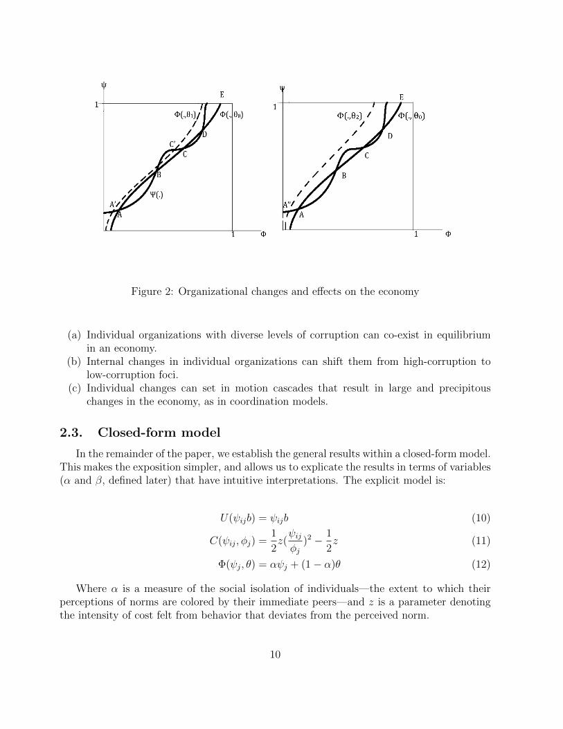
Figure 2: Organizational changes and effects on the economy

(a) Individual organizations with diverse levels of corruption can co-exist in equilibriumin an economy.

(b) Internal changes in individual organizations can shift them from high-corruption tolow-corruption foci.

(c) Individual changes can set in motion cascades that result in large and precipitouschanges in the economy, as in coordination models.

2.3. Closed-form model

In the remainder of the paper, we establish the general results within a closed-form model.This makes the exposition simpler, and allows us to explicate the results in terms of variables(α and β, defined later) that have intuitive interpretations. The explicit model is:

U(ψijb) = ψijb (10)

C(ψij, φj) =1

2z(ψijφj

)2 − 1

2z (11)

Φ(ψj, θ) = αψj + (1− α)θ (12)

Where α is a measure of the social isolation of individuals—the extent to which theirperceptions of norms are colored by their immediate peers—and z is a parameter denotingthe intensity of cost felt from behavior that deviates from the perceived norm.

10

Note that the moral cost C is strictly convex and increasing everywhere in its range.In our formulation it is zero when ψij = φj, i.e., when the official behavior is in line withhis perception of the social norm, and becomes negative when he acts “more morally” thanthe norm. This is in keeping with our interpretation of the cost, though not necessary forthe results. Further, note that given a strictly convex and increasing cost function, a linearutility function does not compromise generality, it is the concavilty of utility net of cost thatdrives the results.

3. Corruption at the department level

In this section we establish the possible organizational foci assuming an exogenous economy-wide average corruption level θ ∈ [0, 1]. The only property of θ that we use in this section isthat it is a weighted average of possible organizational focus levels of ψ, and hence must bea convex combination of these foci.

We show that the number and positions of possible organizational foci depends on therelative value of the parameters α, β and θ (Observation 1). At most, one focus (ψl) isinterior and stable (Lemma 1) where the other interior solution (ψh) acts as an unstabletipping point between total corruption and a low levels of corruption (Corollary 2). Thecorner solution of complete corruption (ψH) is also a possible (Lemma 3) or unique (Lemma4) stable focal point under certain conditions. These are elucidated more formally below.Proofs are in the Appendix.

If the (common) optimization problem of the officials in department j has an interiorsolution then ψj must satisfy

ψj =b

zφ2j (13)

If this yields a value for ψj outside the unit interval, then the corresponding inequalityconditions will apply. Note that different organizations may nevertheless settle at differentstances.

Define β = bz. Given the interpretations of b and z, this exercise is relevant only if β > 0.

Accordingly we assume this is true.

Henceforth we suppress the subscript j when it does not cause confusion. Substituting(13) in (12) and rearranging gives

αβφ2 − φ+ (1− α)θ = 0 (14)

The equation (14) has two roots for φ, given by

φh =1 +

√1− 4α(1− α)βθ

2αβ(15)

φl =1−

√1− 4α(1− α)βθ

2αβ(16)

11

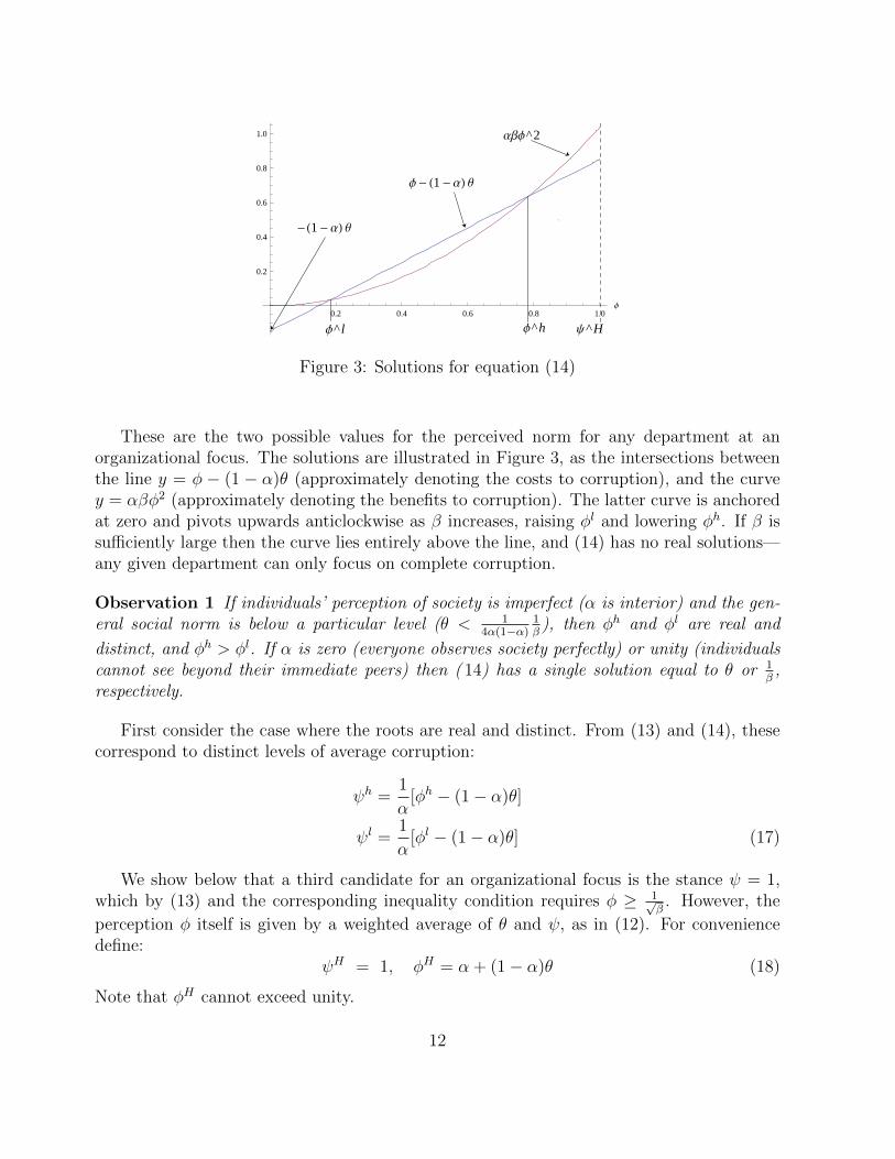
Φ^hΦ^ l

ΑΒΦ^2

Φ - H1 - ΑL Θ

-H1 - ΑL Θ

Ψ^H0.2 0.4 0.6 0.8 1.0

Φ

0.2

0.4

0.6

0.8

1.0

Figure 3: Solutions for equation (14)

These are the two possible values for the perceived norm for any department at anorganizational focus. The solutions are illustrated in Figure 3, as the intersections betweenthe line y = φ − (1 − α)θ (approximately denoting the costs to corruption), and the curvey = αβφ2 (approximately denoting the benefits to corruption). The latter curve is anchoredat zero and pivots upwards anticlockwise as β increases, raising φl and lowering φh. If β issufficiently large then the curve lies entirely above the line, and (14) has no real solutions—any given department can only focus on complete corruption.

Observation 1 If individuals’ perception of society is imperfect (α is interior) and the gen-eral social norm is below a particular level (θ < 1

4α(1−α)1β

), then φh and φl are real and

distinct, and φh > φl. If α is zero (everyone observes society perfectly) or unity (individualscannot see beyond their immediate peers) then ( 14) has a single solution equal to θ or 1

β,

respectively.

First consider the case where the roots are real and distinct. From (13) and (14), thesecorrespond to distinct levels of average corruption:

ψh =1

α[φh − (1− α)θ]

ψl =1

α[φl − (1− α)θ] (17)

We show below that a third candidate for an organizational focus is the stance ψ = 1,which by (13) and the corresponding inequality condition requires φ ≥ 1√

β. However, the

perception φ itself is given by a weighted average of θ and ψ, as in (12). For conveniencedefine:

ψH = 1, φH = α + (1− α)θ (18)

Note that φH cannot exceed unity.

12

Given θ, a solution ψk, (k = l, h,H) with the corresponding perception φk is a candidatefor an organizational focus if both φk and ψk lie in the unit interval.

We can now identify the potential organizational foci as defined in Definition 1. Givenan average economy-wide corruption level θ, an average corruption level ψj ∈ [0, 1] in orga-nization j results in a perception φj = αψj + (1−α)θ, according to (12). Clearly φj ≥ 0. By(13) and the boundary constraints, the optimal ψj corresponding to φj must in turn satisfy

ψj =

{βφ2

j if βφ2j ∈ [0, 1]

1 if βφ2j > 1

A ψj with an associated φj that satisfies the above conditions is a stable focus if it is stablein the sense of Definition 1.

First we address the question of stability. Lemma 1 below shows that, if (14) has real anddistinct solutions, then the lower solution φl corresponds to a stable focus, but the higherone φh does not. In other words, if members of an organization have a (disequilibrium)perception close to φl, then their responses to that perception will lead the organization tosettle at a focus φl. However, if their perception is iclose to (but not equal to) φh, then theircollective responses will lead the organization further away from φh. This follows directlyfrom Lemma 1 below, and is made explicit in the subsequent proposition. All proofs are inthe appendix.

Lemma 1 If both φk and ψk, (k = h, l), lie in the unit interval then ψl is a stable focus,but ψh is not stable.

Proposition 2 (Corollary to Lemma 1) Let ( 14) have real solutions φl and φh, withφl ≤ φh. Suppose an organization currently has a perception φ ∈ [0, 1) with a correspondingstance ψ = β(φ)2. If φ < φl then the stance induces an increase in the perception, ifφ ∈ (φl, φh) then it induces a decrease in the perception, and if φ > φh it induces an increasein the perception.

Note that the formal statement of Proposition 2 does not require that the solutions liein the unit interval. It also does not presuppose that φ is an equilibrium perception.

Since ψh = β(φh)2 is unstable, we will disregard it as a candidate for an organizationalfocus. If ψl < 1 and an organization locates (out of equilibrium) at a corruption stanceψ < ψh, this gives rise to a perception φ < φh, and by Corollary 2 officials in the organizationmust revise their perception and stance downwards until it reaches ψl. Similarly, if ψ > ψh

then the organization must revise upward towards unity, a value of ψ ∈ (ψh, 1) cannot be anorganizational focus. Once the organization reaches a perception ψH = 1, it cannot choosea higher stance. However, ψH can be an organizational focus if θ is sufficiently large, or ifφl is large, as Lemma 3 shows.

Lemma 3 (a) If φl < φH then ψH is a stable organizational focus if and only if β >

max{1, 14α2} and θ ≥ 1−α

√β

(1−α)√β

.

(b) If φl ≥ φH then ψH is a stable organizational focus.

13

φH and ψH were defined in (18) earlier. Extending the argument for part (b) above, it iseasy to see that if β is sufficiently large so that in Figure 3 the curve y = αβφ2 lies entirelyabove the line y = φ− (1− α)θ, then φH is stable against downward deviations, and ψH isthe only possible organizational focus. We summarize this and omit the proof.

Lemma 4 if ( 14) does not have real solutions, then ψH is the unique stable organizationalfocus.

The preceding discussion suggests that there are at most two candidates for stable or-ganizational foci, ψl and ψH . From Lemma 4 it follows that if ψl is not an organizationalfocus, then ψH is a focus, hence at least one focus must exist.

If both foci exist, then organizations in the economy will locate at one or the other, andthe average corruption level θ in the economy will be a weighted average of the two. Wewill state this formally in the next section. For the moment note that since ψH = 1 we haveθ ≤ ψH , so if ψl is also a focus then it must satisfy ψl ≤ θ.

4. A general equilibrium for the economy

The analysis in the previous section leads to the conclusion that there is always at leastone focus on which organizations can coordinate. Depending on the parameters either ψl orψH or both may be potential foci. We will further see below that, for the same parameters(α and β), the economy may have multiple potential sets of foci.8

The equilibrium for the economy is defined by the set of organizational foci, the dis-tribution of organizations between them, and the resulting economy-wide average level ofcorruption θ. If there is only one organizational focus ψ∗ then all organizations will locatethere, and θ must also equal ψ∗. If both ψl and ψH are organizational foci, then individualorganizations will locate at one or the other, and θ will be a weighted average of the two.This leads us to the definition of the economy-wide equilibrium.

Let π = (πl, πH) be the set of employment-weighted fractions of organizations that locateat ψl and ψH respectively, so that πk ≥ 0 for k = l, H and πl + πH = 1.

Definition 2 (Equilibrium) An equilibrium for the economy consists of an aggregate cor-ruption level θ, an associated nonempty set of foci Ψ ⊆ {ψl, ψH}, and a distribution π thatsatisfy:

a. πk > 0, k = l, H only if ψk is an organizational focus given θ.b. θ =

∑k:ψk∈Ψ π

kψk.

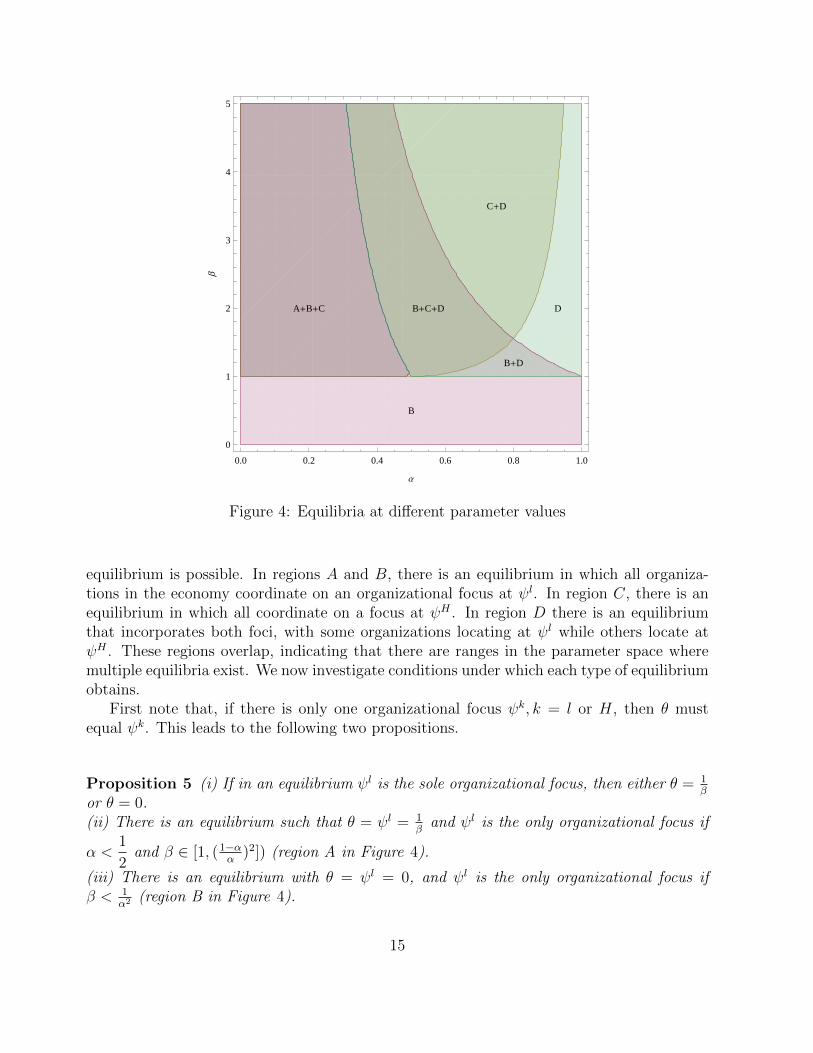
Depending on the values of the parameters α and β, an economy may have three differentkinds of equilibria. Figure 4 shows the regions of the parameter space at which each kind of

8The functional forms chosen produce a saddle shaped map of potential focal points, the shape of whichchanges as θ varies.

14

B

A+B+C B+C+D

C+D

B+D

D

0.0 0.2 0.4 0.6 0.8 1.0

0

1

2

3

4

5

Α

Β

Figure 4: Equilibria at different parameter values

equilibrium is possible. In regions A and B, there is an equilibrium in which all organiza-tions in the economy coordinate on an organizational focus at ψl. In region C, there is anequilibrium in which all coordinate on a focus at ψH . In region D there is an equilibriumthat incorporates both foci, with some organizations locating at ψl while others locate atψH . These regions overlap, indicating that there are ranges in the parameter space wheremultiple equilibria exist. We now investigate conditions under which each type of equilibriumobtains.

First note that, if there is only one organizational focus ψk, k = l or H, then θ mustequal ψk. This leads to the following two propositions.

Proposition 5 (i) If in an equilibrium ψl is the sole organizational focus, then either θ = 1β

or θ = 0.(ii) There is an equilibrium such that θ = ψl = 1

βand ψl is the only organizational focus if

α <1

2and β ∈ [1, (1−α

α)2]) (region A in Figure 4).

(iii) There is an equilibrium with θ = ψl = 0, and ψl is the only organizational focus ifβ < 1

α2 (region B in Figure 4).

15

Proposition 6 There is an equilibrium such that θ = ψH = 1 and ψH is the only organi-

zational focus if either (a) β > 14α(1−α)

or (b) α <1

2and β ∈ (1, 1

2α] (region C in Figure

4).

Finally, we turn to the conditions under which there is an equilibrium with two distinctorganizational foci, ψl and ψH , both with positive weights.

Proposition 7 (Multiple equilibria) If ( 14) has real roots, then there is an equilibriumsuch that both ψl and ψH are organizational foci and a positive fraction of organizationslocate at each focus if either

(i) α <1

2and β > [1−α

α]2, or

(ii) α ≥ 1

2, β > 1.

(region D in Figure 4.)

In summary, an equilibrium is the set of the stable organizational foci, the proportion ofdepartments at each focus, and the resulting average corruption level. At given parametervalues, an equilibrium is comprised of either a unique interior focal point for all organizations(Proposition 6), a unique focal point at complete corruption for all organizations (Proposition7) or both of these with a proportion of organizations focusing on each (Proposition 8).

Multiple equilibria can exist for a wide range of parameter values. For example in figure 4,if α and β are in the region marked B+C+D, there is an equilibrium in which all organizationssettle at a focus with ψ = 0 (Proposition 5), an equilibrium in which all organizations focuson ψ = ψH = 1 (Proposition 6), and an equilibrium in which some organizations settle atan interior level ψl while others settle at ψH (Proposition 7).

In particular, in Proposition 7, we have our description of an equilibrium in which other-wise identical departments in the same economy focus on very different patterns of corruptbehavior. The possibility of this state is determined by prevailing incentives and the degreeof social isolation, and its existence is determined by officials’ perceptions of the rest of so-ciety. In the state where it does exist, the level of corrupt behavior on which a particularorganization focuses will be determined by officials’ perceptions of their colleagues’ beliefs,as discussed in Section 3. Hence in this equilibrium we can see how distinct organizationalcultures might establish and persist over time in an economy with uniform incentives andhomogeneous agents.

5. Conclusion and policy implications

Whereas most economic corruption models focus on structural incentives, our modelinvestigates how peer effects can produce different but persistent cultures of corruption. Weexamine officials’ decisions when they must contend with their own personal morals and

16

also their perceptions of what is normal. We find multiple organizational foci can exist.Furthermore it is feasible for these foci to persist over time in the economy as officials’perceptions and decisions create organizational cultures that propagate the behavior.

It should be emphasized that we used a simple model, and hence derived correspondinglystark results. However, many of the simplifications generalize readily. In particular, we drawattention to one consequence of our simplifications; in any equilibrium, each official in each ofthe organizations located at a given focus is corrupt to exactly the same degree. As a result,all of these organizations are equally corrupt. Clearly this will not be the case if differentofficials in the same department have (i) different levels of exposure to the broader economy(i.e., different αs) and (ii) different moral costs z for deviating from what they consider thetrue moral line, and (iii) different opportunities for corruption (different bijs). If this is thecase, then even within a department each official will avail his corruption opportunities to adifferent degree, and indeed the departments located near a given focus will in fact displaydifferent average levels of corruption. Further, the actual perceived levels of corruption indifferent departments will vary according to the vantage point of the observer (whether shedealt with a more or less corrupt official). Admitting such variations does not compromisethe validity of our model.

It is of greater importance to note that our analysis provides very definite and sometimesnovel perspectives on policy. Consider an economy in an equilibrium with high levels of cor-ruption, either because total corruption is the only organizational focus or because there aremultiple foci and a high proportion of organizations have settled on this option. Our resultssuggest four linked implications that could inform anti-corruption policy in this economy:

1. In accordance with preceding literature, reducing the relative benefits of corruption(i.e., reducing β by decreasing the rewards of corruption b or increasing its cost z) willreduce corruption. The mechanism at work here is that as the benefits are reduced, thepossible equilibria change: in extreme cases (where the benefits to corruption are all buteliminated) the possibility of a highly corrupt focal point in equilibrium is completelyremoved. In other cases, reducing the benefits to corruption may introduce a tippingpoint (φh < φH) below which organizations will focus on lower levels of corruption. Asreductions continue further, this tipping point will increase to higher levels and thusmore corrupt organizations will fall below it. In either case, aggregate corruption willdecrease.

2. In the equilibrium with two focal points, significant changes in departmental corruptionlevels may be brought about with no change to the incentive structure but rather bytargeting the social-psychological mechanisms discussed earlier. That is, significantimprovements within organizations may be achieved by policies that aim to disruptthe corrupt subcultures. For example, targeting individuals’ perceptions of what thenorm is by discrediting prevalent rationalizations for the behavior will increase themoral costs individuals bear and could effect an organizational switch from the higher

17

to lower focal points. These policies will be more effective if the tipping point is higher,because they only need to push bureaucrats’ expectations of others’ behavior acrossthat line, rather than drive them down all the way to the lower equilibrium.

3. This gives rise to the key observation that the battle to reduce corruption in an economyoverall can be won by whittling away at the cultures of individual departments oneat a time, rather than with a big push against all departments at once. In fact, bytargeting policies such as those discussed above at particular (and particularly visible)organizations, policymakers may effect a change in the proportion of organizationsfocusing on the higher focal point in the equilibrium with two foci. At the margin,the structure of the equilibrium changes, so that complete corruption is no longer asustainable focus for any department, regardless of whether they have been targetedby reform programs.

4. Finally, note that in Proposition 7, organizations may congregate at the high corruptionequilibrium even when incentives are relatively weak (β > 1) if their degree of socialisolation is high (α > 1

2). Here departmental corruption is driven largely by internal

culture, not the state of corruption in the broader economy. Providing officials witha truer perception of the prevailing social norm will here be effective in shifting thedepartment away from its prevailing focus. However, this is a delicate instrument,since in the departments located at the low corruption focus the same policy wouldhave precisely the opposite effect.

In conclusion, we draw attention to our interpretation of the assumption regarding thecost of corruption. Our interpretation is that the decision to be corrupt is not entirely afunction of narrowly economic costs and benefits, it is also in large part driven by moralfactors that derive their force from social norms, which in turn are formed by common andaccepted practice. We believe that incorporating this aspect of the decision in economicmodelling of the phenomenon of corruption is potentially beneficial for policy formulation.

References

Akerlof, George (1976), ‘The economics of caste and of the rat race and other woeful tales’,The Quarterly Journal of Economics 90(4), 599–617.

Akerlof, George A. and William T. Dickens (1982), ‘The economic consequences of cognitivedissonance’, The American Economic Review 72(3), 307–319.

Andvig, Jens Chr and Karl Ove Moene (1990), ‘How corruption may corrupt’, Journal ofEconomic Behavior & Organization 13(1), 63–76.

Arendt, Hannah (1977), Eichmann in Jerusalem: a report on the banality of evil, PenguinBooks, London.

18

Ashforth, Blake E. and Vikas Anand (2003), ‘The normalization of corruption in organiza-tions’, Research in Organizational Behavior 25, 1–52.

Bardhan, Pranab (1997), ‘Corruption and development: A review of issues’, Journal ofEconomic Literature 35(3), 1320–1346.

Basu, Kaushik (2000), Prelude to Political Economy: A Study of the Political Foundationsof Economics, Oxford: Oxford University Press.

Blackburn, Keith, Niloy Bose and M. Emranul Haque (2006), ‘The incidence and persis-tence of corruption in economic development’, Journal of Economic Dynamics & Control30, 2447–2467.

Bose, Gautam and Shubhashis Gangopadhyay (2009), ‘Intermediation in corruption mar-kets’, Indian Growth and Development Review 2(1), 39–55.

Coleman, James S. (1990), Foundations of Social Theory, Harvard University Press, Cam-bridge, MA.

Cressey, Donald R. (1971), Other People’s Money: A study in the social psychology of em-bezzlement, Wadsworth, Belmont, CA.

Elster, Jon (1989), ‘Social norms and economic theory’, The Journal of Economic Perspec-tives 3(4), 99–117.

Fischer, Paul and Steven Huddart (2008), ‘Optimal contracting with endogenous socialnorms’, American Economic Review 98(4), 1459–75.

Glaeser, Edward L, Bruce Sacerdote and Jose A Scheinkman (1996), ‘Crime and socialinteractions.’, Quarterly Journal of Economics 111(2).

Ichino, Andrea and Giovanni Maggi (2000), ‘Work environment and individual background:explaining regional shirking differentials in a large italian firm’, The Quarterly Journal ofEconomics 115(3), 1057–1090.

Klitgaard, Robert E. (1988), Controlling Corruption, University of California Press, Berkeleyand Los Angeles, CA.

Laub, John H. (2006), ‘Edwin H. Sutherland and the Michael-Adler Report: Searching forthe soul of criminology seventy years later’, Criminology 44(2), 235–257.

Murphy, Kevin M., Andrei Shleifer and Robert W. Vishny (1993), ‘Why is rent-seeking socostly to growth?’, The American Economic Review 83(2), 409–414.

Nabin, Munirul Haque and Gautam Bose (2008), ‘Partners in crime: Collusive corruptionand search’, The B.E. Journal of Economic Analysis & Policy 8(1).

19

Rabin, Matthew (1994), ‘Cognitive dissonance and social change’, Journal of EconomicBehavior & Organization 23, 177–194.

Rasmusen, Eric (1996), ‘Stigma and self-fulfilling expectations of criminality’, Journal ofLaw and Economics pp. 519–543.

Sardan, J. P. Olivier de (1999), ‘A moral economy of corruption in Africa?’, The Journal ofModern African Studies 37(1), 25–52.

Schneider, Patrick (2011), Everyone was doing it: Culture, Rationalisation and Corruption,Honours thesis, School of Economics, University of New South Wales, Sydney.

Wade, Robert (1982), ‘The system of administrative and political corruption: Canal irriga-tion in South India’, Journal of Development Studies pp. 287–328.

Wade, Robert (1985), ‘The market for public office: why the indian state is not better atdevelopment’, World Development 13(4), 467–497.

Appendix A Proofs

Proof of Lemma 1

Suppose that both φl and φh lie in the unit interval. Consider a perceived corruption levelφ = φk + ∆, ∆ 6= 0 that deviates by a small amount ∆ from one of the solutions. Given θ,this leads to a choice of corruption level ψ = βφ2 = β[(φk)2 + 2∆φk + ∆2]. In conjunctionwith θ, ψ must in turn give rise to a new perception φ′ = αβ[(φk)2 + 2∆φk + ∆2] + (1−α)θ,which reduces to φ′ = αβ[2∆φk + ∆2] + φk using (14). The perception φk is stable if

|φ′ − φk| < |φ− φk|⇒ |2αβ∆φk + αβ∆2| < |∆|⇒ |2αβφk + αβ∆| < 1 (19)

which in the limit as ∆→ 0 requires 2αβφk < 1. It follows immediately from (15) and (16)that the smaller solution φl is stable while the larger, φh, is not. �

Proof of Lemma 3

(a) First, by (13), for ψH to be an optimal stance the corresponding perception must satisfyβ(φH)2 > 1 which implies φH ≥ 1√

β. However, according to (18) φH = φ = α + (1 − α)θ.

This exceeds 1√β

if and only if θ ≥ 1−α√β

(1−α)√β.

Next, the perception φH is stable against upward perturbations because ψ cannot exceedunity. Since φl < φH , by Corollary 2 ψH is stable against downward deviations only ifφh < φH . By the earlier part of the proof, a sufficient condition for this is φh < 1√

β.

20

From (15), φh < 1√β⇔

√1− 4α(1− α)βθ < 2α

√β− 1. Since the LHS is positive (real

roots) the RHS must be positive, which requires β > 14α2 . Squaring both sides then again

yields θ ≥ 1−α√β

(1−α)√β, hence the necessary condition for ψH = 1 is sufficient for φh < φH .

Finally, note that θ ≥ 1−α√β

(1−α)√β

requires that 1−α√β

(1−α)√β< 1, for which either β > 1 or the

numerator is non-positive implying β > 1α2 > 1. Thus β must in fact exceed max{1, 1

4α2}.(b) Follows from Corollary 2. �

Lemma 8 When ( 14) has real roots, ψl ≤ θ if either (i) α ≥ 1

2or (ii) θ ≤ 1

β.

Proof of Lemma 8

From (12) it follows that ψl ≤ θ if and only if φl ≤ θ. From (16), this requires√1− 4α(1− α)βθ ≥ 1− 2αβθ

It follows that:(a) If θ < 1

2αβthen the RHS is positive, squaring both sides and simplifying yields θ < 1

β.

(b) If θ ≥ 12αβ

then the RHS is non-positive and the condition is satisfied.

Note also:(c) θ ≥ 1

2αβimplies 4α(1−α)βθ ≥ 2(1−α). Real roots require 4α(1−α)βθ ≤ 1 so we must

have 2(1− α) ≤ 1 or α ≥ 1

2.

(d) 1βQ 1

2αβas α S

1

2.

(i) Let α ≥ 1

2. Then 1

β≥ 1

2αβ. So if θ < 1

2αβthen θ < 1

βand φl < θ by (a), and if θ ≥ 1

2αβ

and (14) has real roots then φl < θ by (b).

(ii) By the first part of (i), θ < 1β→ φl < θ if α ≥ 1

2. If α <

1

2, then 1

β< 1

2αβby (d), so

θ < 1β⇒ φl < θ by (a).

Further, if α <1

2and θ ≥ 1

2αβthen (14) does not have real roots by (c), so (b) does not

apply. �

Proof of Proposition 5

(i) Since φl is a convex combination of θ and ψl, if ψl is the only O-equilibrium then we musthave θ = ψl = φl ⇒ β(φl)2 = φl which implies φl = 0 or 1

β.

(ii) Let θ = φl = ψl = 1β, which implies that β ≥ 1. When θ = 1

β, the two roots of (14

are 1β

and 1−ααβ

. Since we want φl = 1β

we need this to be the smaller root, which implies

21

α <1

2. Further we need that ψH is not an organizational focus, by Lemma 3, a necessary

and sufficient condition for this is θ = 1β< 1−α

√β

(1−α)√β

which reduces to β ≤ (1−αα

)2. 9

(iii) If θ = φl = ψl = 0 is the only equilibrium then ψH is not an equilibrium, so we musthave φh ≥ φH . Given that θ = 0, we have φH = α and φh = 1

αβ. Hence the required

condition is

φh ≥ φH ⇔ 1

αβ≥ α ⇔ β ≤ 1

α2

�

Proof of Proposition 6

Let θ = 1. If condition (a) is satisfied then (14) has no real roots hence there are no solutionsother than ψH , so the latter is an equilibrium. If (a) is not satisfied then we need φl ≥ 1 toensure that ψH is the only equilibrium. Using (16) and θ = 1, this condition is equivalentto

√1− 4α(1− α)β ≤ 1 − 2αβ. Since the LHS is non-negative we must have the RHS

non-negative as well which requires β ≤ 12α

. Squaring both sides then yields β > 1, so we

must also have α <1

2. �

Proof of Proposition 7

Note (a) since θ is a convex combination of ψl and ψH , and ψH = 1 > θ, we must have

ψl < θ. Therefore by Lemma 8 either α <1

2and θ < 1

β, or α ≥ 1

2.

Further, (b) ψH must be a stable equilibrium, so by Lemma 3 we need θ > 1−α√β

(1−α)√β

and

β > max{1, 14α2}.

(i) Let α <1

2. We need 1−α

√β

(1−α)√β< θ < 1

β. Some manipulation gives 1

β> 1−α

√β

(1−α)√β⇔ β >

[1−αa

]2. Note that if β > 1 then 1β∈ (0, 1) and hence 1−α

√β

(1−α)√β< 1, so the interval has a non-

empty intersection with the range of θ. Further, since α <1

2⇒ α2 < 1

4so max{1, 1

4α2} = 1,

In turn 1−αa

]2 > 1 so the condition on β in (b) is satisfied. Now pick θ ∈ ( 1−α√β

(1−α)√β, 1β), and

define πθ = 1−θ1−ψl which implies θ = πθψ

l + (1 − πθ)ψH . Then {Ψ, πθ, θ} is an equilibrium

with Ψ = {ψl, ψH}.

(ii) Let α ≥ 1

2. Then max{1, 1

4α2} = 1 so β > 1 satisfies the condition on β in (b). In turn

this ensures that 1−α√β

(1−α)√β< 1. By (a) we have ψl < θ. So pick θ ∈ ( 1−α

√β

(1−α)√β, 1), and define

πθ as before, then {Ψ, πθ, θ} is an equilibrium with Ψ = {ψl, ψH}. �

9An equivalent statement of (ii) is “There is an equilibrium such that θ = ψl = 1β and ψl is the only

organizational focus if β > 1 and α < 11+√β

”

22

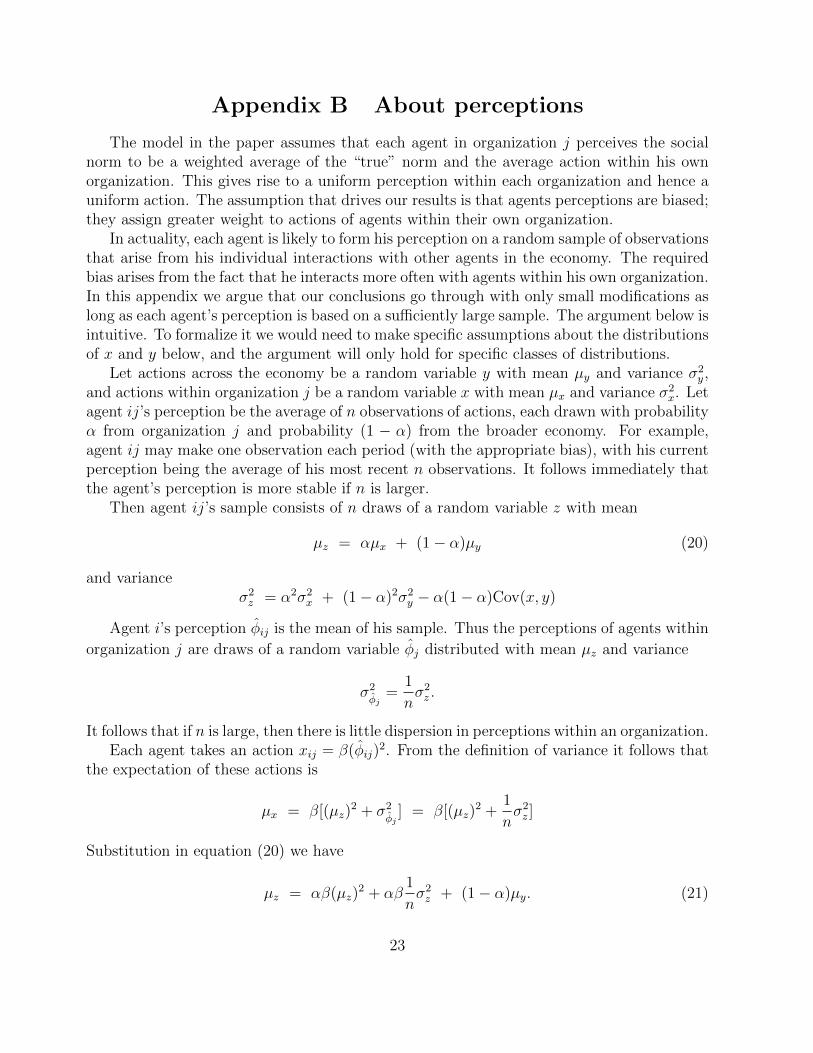
Appendix B About perceptions

The model in the paper assumes that each agent in organization j perceives the socialnorm to be a weighted average of the “true” norm and the average action within his ownorganization. This gives rise to a uniform perception within each organization and hence auniform action. The assumption that drives our results is that agents perceptions are biased;they assign greater weight to actions of agents within their own organization.

In actuality, each agent is likely to form his perception on a random sample of observationsthat arise from his individual interactions with other agents in the economy. The requiredbias arises from the fact that he interacts more often with agents within his own organization.In this appendix we argue that our conclusions go through with only small modifications aslong as each agent’s perception is based on a sufficiently large sample. The argument below isintuitive. To formalize it we would need to make specific assumptions about the distributionsof x and y below, and the argument will only hold for specific classes of distributions.

Let actions across the economy be a random variable y with mean µy and variance σ2y,

and actions within organization j be a random variable x with mean µx and variance σ2x. Let

agent ij’s perception be the average of n observations of actions, each drawn with probabilityα from organization j and probability (1 − α) from the broader economy. For example,agent ij may make one observation each period (with the appropriate bias), with his currentperception being the average of his most recent n observations. It follows immediately thatthe agent’s perception is more stable if n is larger.

Then agent ij’s sample consists of n draws of a random variable z with mean

µz = αµx + (1− α)µy (20)

and varianceσ2z = α2σ2

x + (1− α)2σ2y − α(1− α)Cov(x, y)

Agent i’s perception φij is the mean of his sample. Thus the perceptions of agents within

organization j are draws of a random variable φj distributed with mean µz and variance

σ2φj

=1

nσ2z .

It follows that if n is large, then there is little dispersion in perceptions within an organization.Each agent takes an action xij = β(φij)

2. From the definition of variance it follows thatthe expectation of these actions is

µx = β[(µz)2 + σ2

φj] = β[(µz)

2 +1

nσ2z ]

Substitution in equation (20) we have

µz = αβ(µz)2 + αβ

1

nσ2z + (1− α)µy. (21)

23

Recall that µz = E(φj) is the mean of the organization’s perceptions. The model in thepaper assumes that all agents in j have the same perception φj. µy is the mean action inthe economy, or θ in the notation of the model. If n is very large so that we can ignore thesecond term on the right-hand-side of (21), then equation (21) reduces to equation (14), andwe recover the model in the paper. For finite n, equation (14) has an extra additive termαβ 1

nσ2z , which yields solutions that are close to those for (14) if n is large.

In particular, consider a stable focus φj of the economy yielded by a solution for equation(14). Then there is a neighborhood N(φj) of φj such that a small displacement in perceptionwill result in dynamics that correct this displacement (see Definition 1). If n is large enough,then the corresponding solution for µz in (21) is in the interior of N(φj). Further as n −→∞,

µz −→ φj and σ2φj−→ 0. Hence for any p ∈ (0, 1), there is n such that prob{φij /∈ N(φj)} <

p. Hence with probability (1− p)Nj the perceptions of all Nj agents in j remain close to φj.The arguments in the paper go through with this slightly modified conceptions of focus andstability.

Conversely, for any n and k we can calculate the probability that k or more membersof j will develop perceptions outside N(φj). It seems a reasonable conjecture that the or-ganization’s “culture” will be disrupted if several of the agents have perceptions outside thestable neighborhood. This may have implications for anti-corruption policy. For example,a perception that “things are changing” as a result of anti-corruption initiatives may leadagents to disregard observations made in the past, and hence reduce the number of obser-vations on which perceptions are based. This would make perceptions more volatile, andhence organizational cultures more prone to breaking down.

24