Organisations, C2-Entropy and Military CommandDr Alexander KalloniatisJoint Operations Division

13th ICCRTS “C2 for Complex Endeavours”Seattle, WA, USAJune 17-19 2008

Outline

0. The elements of C2-Entropy1. Historical Motivation2. Theoretical Development of C2-Entropy

Concept3. Return to History4. Implications for Future C2(Appendix: Supplementary Material)

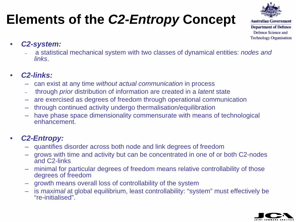
Elements of the C2-Entropy Concept• C2-system:

– a statistical mechanical system with two classes of dynamical entities: nodes and links.

• C2-links:– can exist at any time without actual communication in process– through prior distribution of information are created in a latent state– are exercised as degrees of freedom through operational communication– through continued activity undergo thermalisation/equilibration– have phase space dimensionality commensurate with means of technological

enhancement.

• C2-Entropy:– quantifies disorder across both node and link degrees of freedom– grows with time and activity but can be concentrated in one of or both C2-nodes

and C2-links– minimal for particular degrees of freedom means relative controllability of those

degrees of freedom– growth means overall loss of controllability of the system– is maximal at global equilibrium, least controllability: “system” must effectively be

“re-initialised”.

1. Historical Motivation

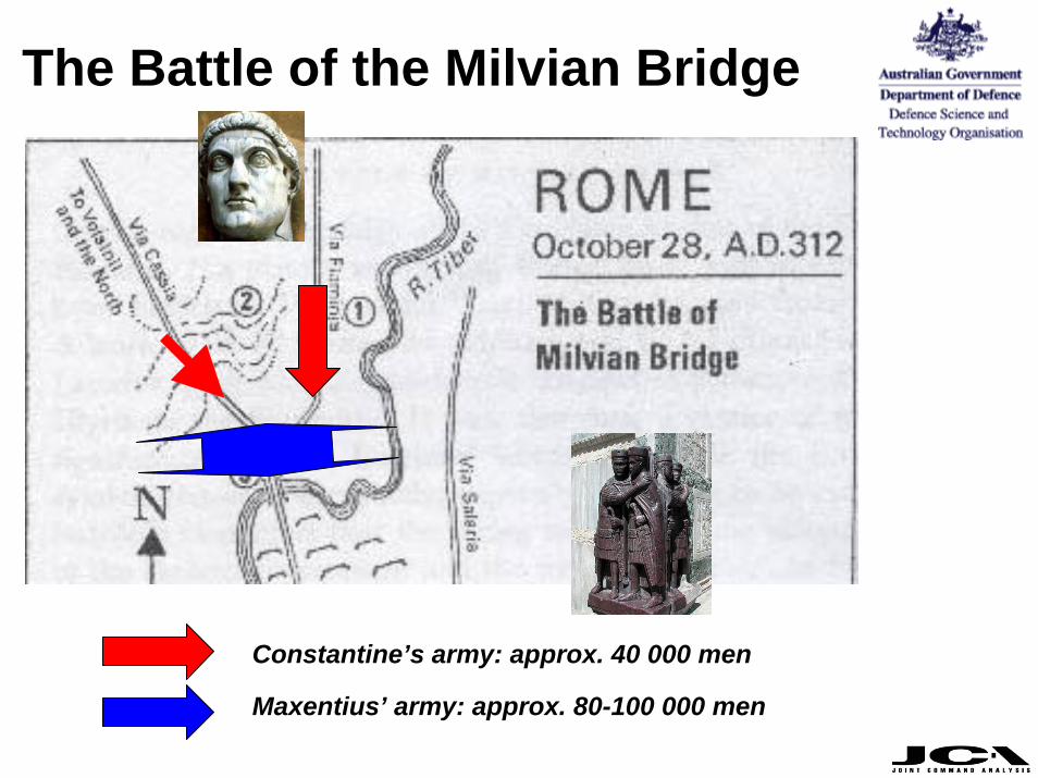
Constantine’s army: approx. 40 000 men

Maxentius’ army: approx. 80-100 000 men

The Battle of the Milvian Bridge

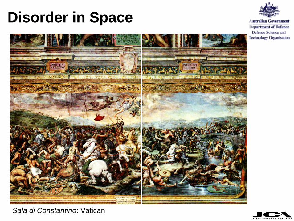
Disorder in Space

Sala di Constantino: Vatican

Irreversibility in War

“… as long as Maxentius’ cavalry offered resistance there seemed some hope left for him. But when his horsemen gave up he took to flight along with the rest and made for the city via the bridge acrossthe river the timbers could not sustain the pressure of the host, but broke …”

Zosimus, Historia Nova

= Maxentius’ defeat was irreversible after capitulation of cavalry.

…… there is no other general measure for the irreversibility of a there is no other general measure for the irreversibility of a process than the amount of increase in entropy.process than the amount of increase in entropy.

Max Planck, 1905.

C2 and Maxentius’ Defeat

• Entropy of Maxentius’ army increased with time: spatial disorder.

• C2-system was available (Roman military doctrine, chain of command, primitive comms) but not used.

• C2 can reverse spatial disorder – does this contradict growing entropy?

• Not necessarily: C2 degrees of freedom are part of the system.

2. Theoretical Considerations

Command and Control

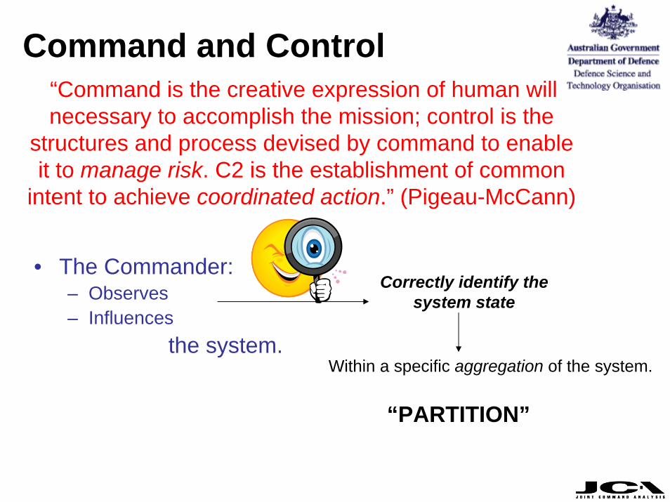
• The Commander: – Observes– Influences

the system.

“Command is the creative expression of human will necessary to accomplish the mission; control is the

structures and process devised by command to enable it to manage risk. C2 is the establishment of common

intent to achieve coordinated action.” (Pigeau-McCann)

Correctly identify the system state

Within a specific aggregation of the system.

“PARTITION”

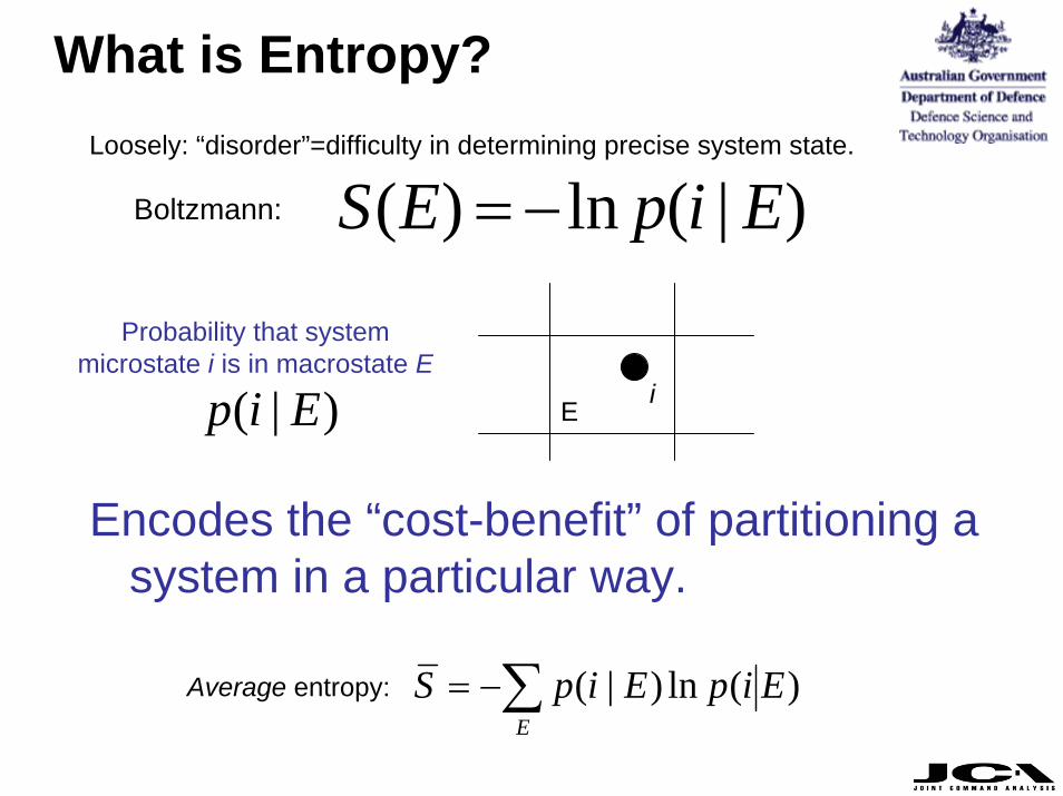
What is Entropy?

Encodes the “cost-benefit” of partitioning a system in a particular way.

)(ln)|( EipEipSE∑−=

Ei

)|(ln)( EipES −=

)|( Eip

Probability that system microstate i is in macrostate E

Average entropy:

Boltzmann:

Loosely: “disorder”=difficulty in determining precise system state.

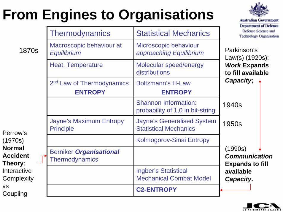
From Engines to OrganisationsThermodynamics Statistical MechanicsMacroscopic behaviour at Equilibrium

Microscopic behaviour approaching Equilibrium

Heat, Temperature Molecular speed/energy distributions

2nd Law of ThermodynamicsENTROPY

Boltzmann’s H-LawENTROPY

Shannon Information: probability of 1,0 in bit-string

Jayne’s Maximum Entropy Principle

Jayne’s Generalised System Statistical Mechanics

Kolmogorov-Sinai Entropy

Berniker Organisational Thermodynamics

Ingber’s Statistical Mechanical Combat Model

C2-ENTROPY

Perrow’s(1970s)Normal Accident Theory:Interactive Complexity vsCoupling

Parkinson’s Law(s) (1920s):Work Expands to fill available Capacity;

(1990s)CommunicationExpands to fill available Capacity.

1940s

1950s

1870s

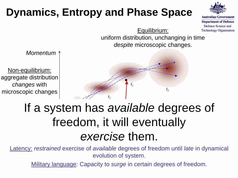
Dynamics, Entropy and Phase Space

Momentum

Position1 axis for each cptand for each system entity

Equilibrium:uniform distribution, unchanging in time

despite microscopic changes.

Non-equilibrium: aggregate distribution

changes with microscopic changes

Entropy:roughly, the spread of distribution

about actual system state

System state:a point in phase (or state) space.

If a system has available degrees of freedom, it will eventually

exercise them.Latency: restrained exercise of available degrees of freedom until late in dynamical

evolution of system.Military language: Capacity to surge in certain degrees of freedom.

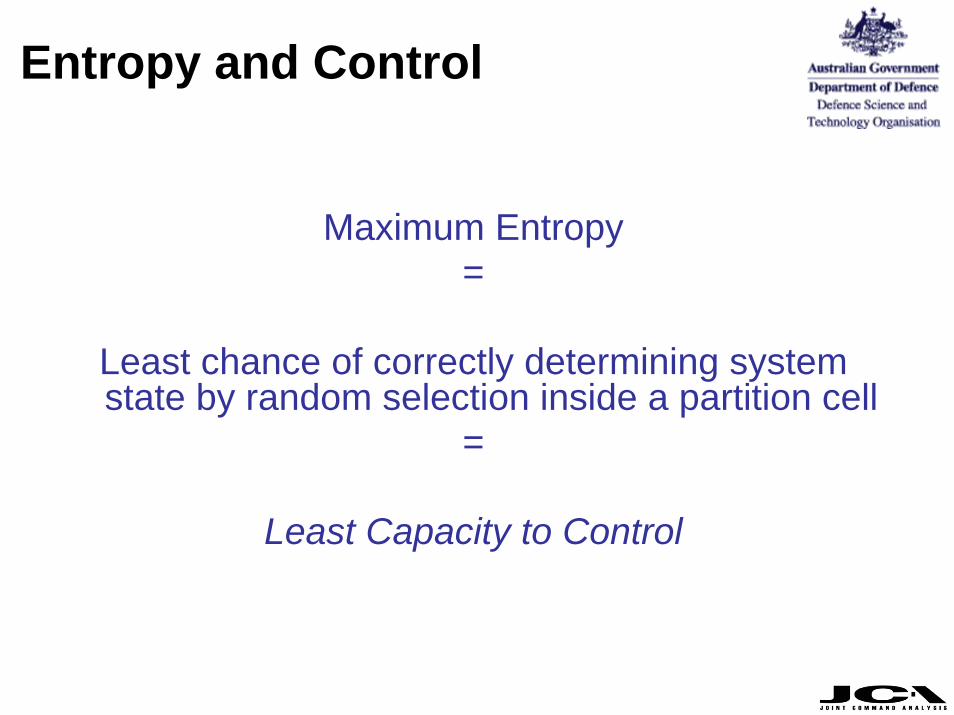
Entropy and Control

Maximum Entropy=

Least chance of correctly determining system state by random selection inside a partition cell

=

Least Capacity to Control

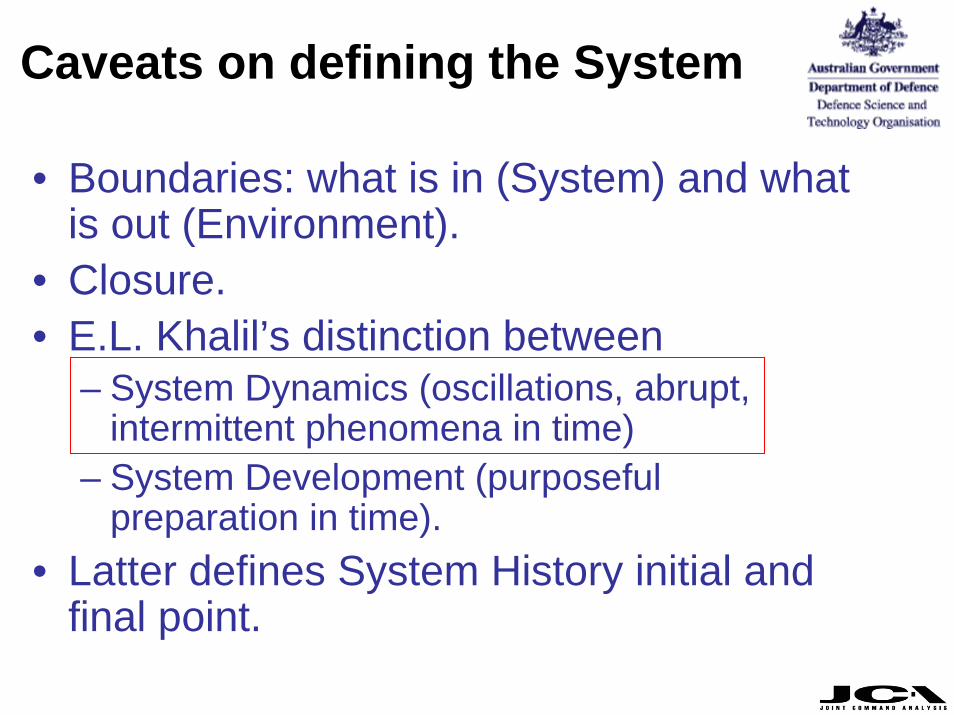
Caveats on defining the System

• Boundaries: what is in (System) and what is out (Environment).

• Closure.• E.L. Khalil’s distinction between

– System Dynamics (oscillations, abrupt, intermittent phenomena in time)

– System Development (purposeful preparation in time).

• Latter defines System History initial and final point.

3. Back to History

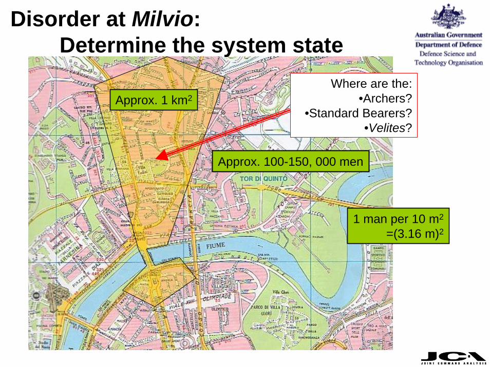
Approx. 100-150, 000 men

Approx. 1 km2

1 man per 10 m2

=(3.16 m)2

Disorder at Milvio: Determine the system state

Where are the:•Archers?

•Standard Bearers?•Velites?

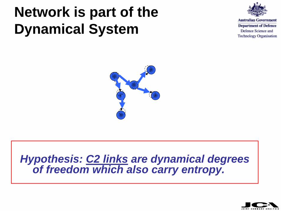
Network is part of the Dynamical System

Hypothesis: C2 links are dynamical degrees of freedom which also carry entropy.

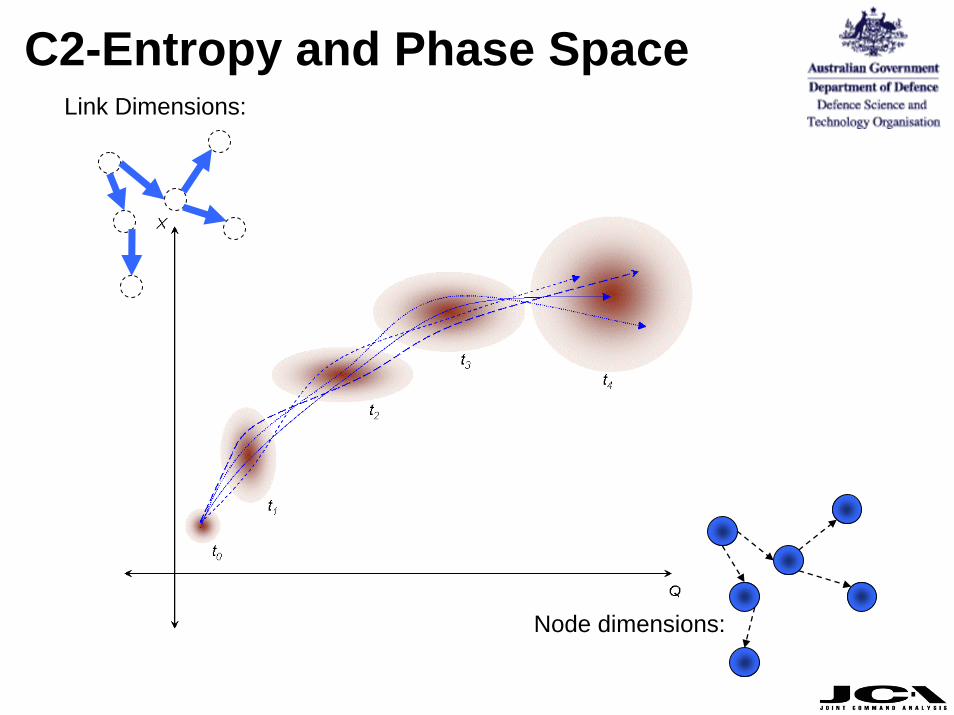
C2-Entropy and Phase SpaceLink Dimensions:

Node dimensions:

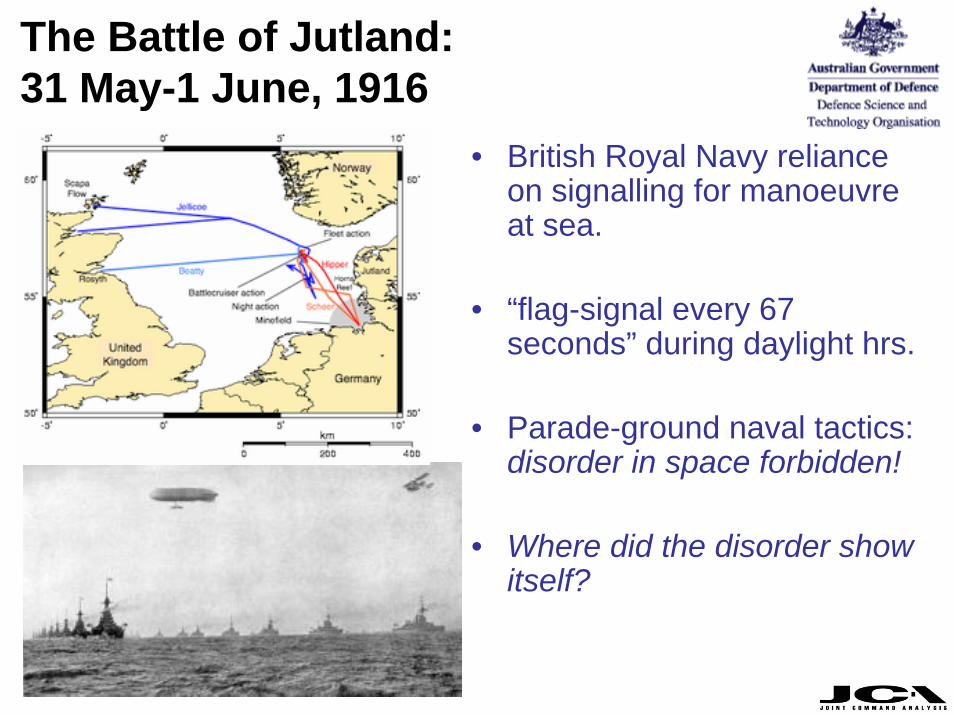
The Battle of Jutland: 31 May-1 June, 1916

• British Royal Navy reliance on signalling for manoeuvre at sea.

• “flag-signal every 67 seconds” during daylight hrs.

• Parade-ground naval tactics: disorder in space forbidden!

• Where did the disorder show itself?

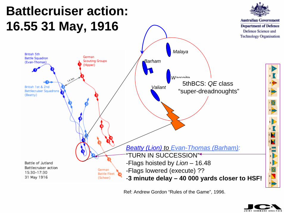
Battlecruiser action: 16.55 31 May, 1916

Beatty (Lion) to Evan-Thomas (Barham):“TURN IN SUCCESSION”-Flags hoisted by Lion – 16.48-Flags lowered (execute) ??-3 minute delay – 40 000 yards closer to HSF!

Barham

Valiant

Warspite

Malaya

Ref: Andrew Gordon “Rules of the Game”, 1996.

5thBCS: QE class “super-dreadnoughts”

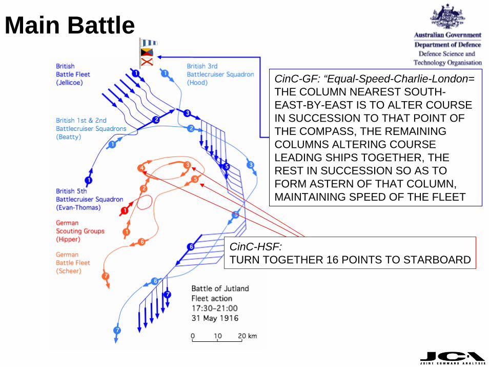
Main Battle

CinC-GF: “Equal-Speed-Charlie-London=THE COLUMN NEAREST SOUTH-EAST-BY-EAST IS TO ALTER COURSE IN SUCCESSION TO THAT POINT OF THE COMPASS, THE REMAINING COLUMNS ALTERING COURSE LEADING SHIPS TOGETHER, THE REST IN SUCCESSION SO AS TO FORM ASTERN OF THAT COLUMN, MAINTAINING SPEED OF THE FLEET

CinC-HSF:TURN TOGETHER 16 POINTS TO STARBOARD

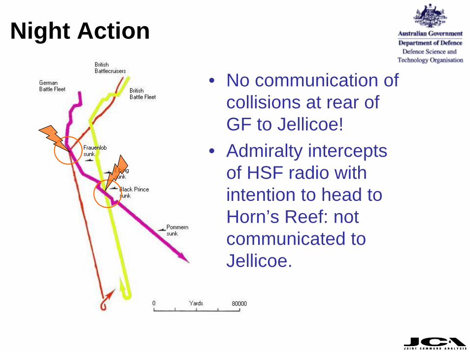
Night Action

• No communication of collisions at rear of GF to Jellicoe!

• Admiralty intercepts of HSF radio with intention to head to Horn’s Reef: not communicated to Jellicoe.

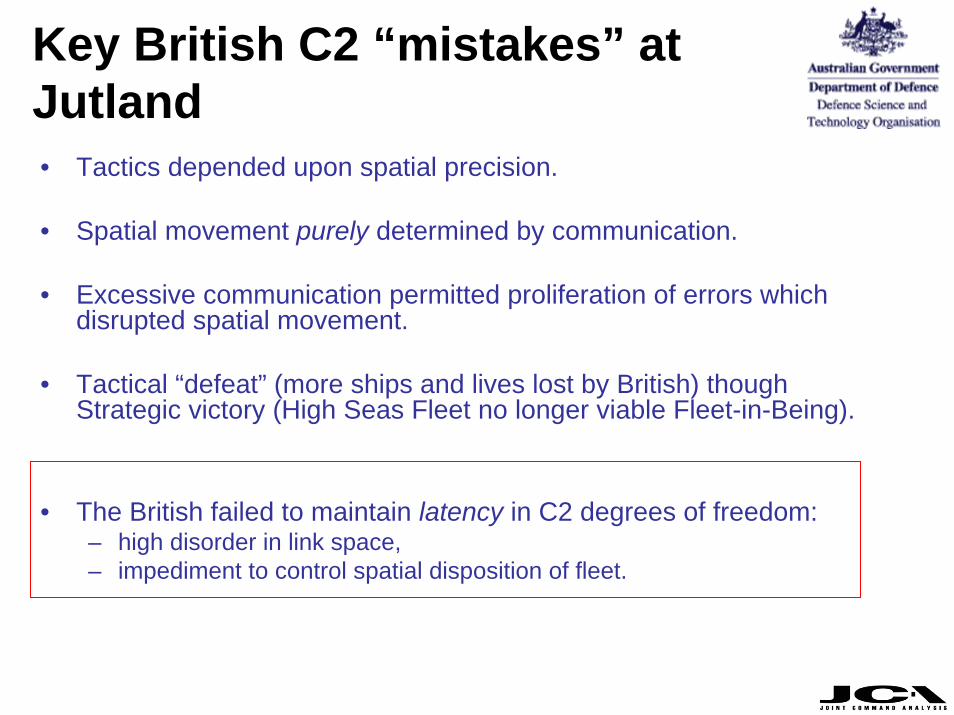
Key British C2 “mistakes” at Jutland• Tactics depended upon spatial precision.

• Spatial movement purely determined by communication.

• Excessive communication permitted proliferation of errors which disrupted spatial movement.

• Tactical “defeat” (more ships and lives lost by British) though Strategic victory (High Seas Fleet no longer viable Fleet-in-Being).

• The British failed to maintain latency in C2 degrees of freedom: – high disorder in link space, – impediment to control spatial disposition of fleet.

4. Implications for the Future Command and Control

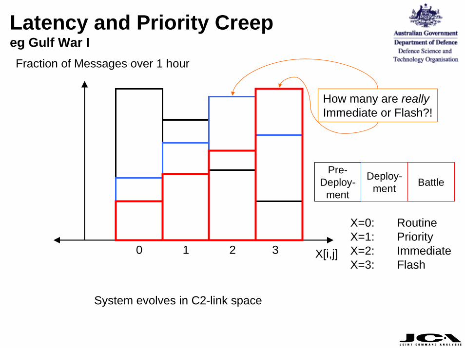
Latency and Priority Creepeg Gulf War I

X[i,j]

Fraction of Messages over 1 hour

0 1 2

X=0: RoutineX=1: PriorityX=2: ImmediateX=3: Flash

3

Pre-Deploy-

ment

Deploy-ment Battle

How many are really Immediate or Flash?!

System evolves in C2-link space

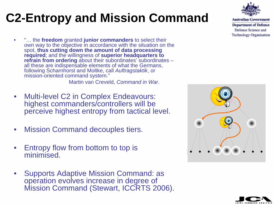
C2-Entropy and Mission Command• “… the freedom granted junior commanders to select their

own way to the objective in accordance with the situation on thespot, thus cutting down the amount of data processing required; and the willingness of superior headquarters to refrain from ordering about their subordinates’ subordinates –all these are indispensable elements of what the Germans, following Scharnhorst and Moltke, call Auftragstaktik, or mission-oriented command system.”

Martin van Creveld, Command in War.

• Multi-level C2 in Complex Endeavours: highest commanders/controllers will be perceive highest entropy from tactical level.

• Mission Command decouples tiers.

• Entropy flow from bottom to top is minimised.

• Supports Adaptive Mission Command: as operation evolves increase in degree of Mission Command (Stewart, ICCRTS 2006).

Lessons for NCW

• Technologically enhanced C2: Vast numbers of degrees of freedom.

• Disorder is a necessary evil.

• How to “deal with it”:– structured use of C2 degrees of freedom, – channel appropriately between nodes and links,– Maintain capacity to surge (latency) in those degrees of freedom.

• The C2-Entropy Concept:

– C2-Entropy is a construct to manage disorder in a C2-system by channelling between node and link degrees of freedom in order to make the system flexible/adaptable.

5. Supplementary Material

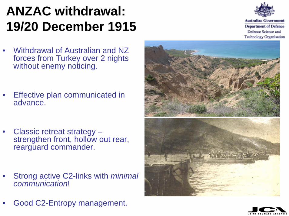
ANZAC withdrawal: 19/20 December 1915

• Withdrawal of Australian and NZ forces from Turkey over 2 nights without enemy noticing.

• Effective plan communicated in advance.

• Classic retreat strategy –strengthen front, hollow out rear, rearguard commander.

• Strong active C2-links with minimal communication!

• Good C2-Entropy management.

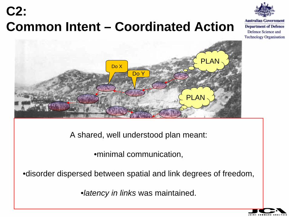
C2: Common Intent – Coordinated Action

Do XDo Y

PLAN

PLAN

A shared, well understood plan meant:

•minimal communication,

•disorder dispersed between spatial and link degrees of freedom,

•latency in links was maintained.

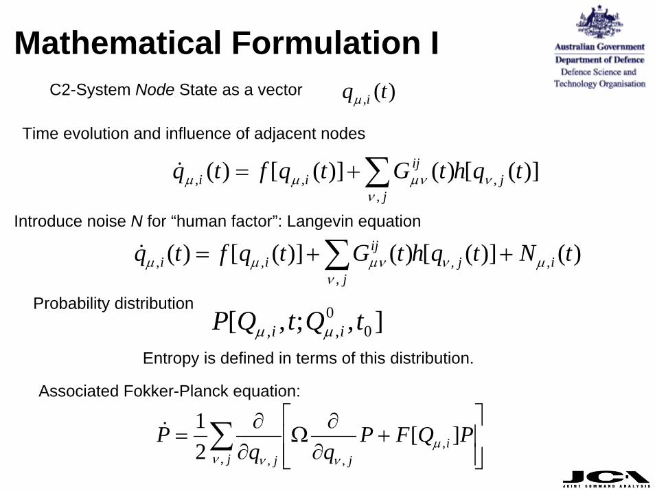
Mathematical Formulation IC2-System Node State as a vector )(, tq iμ

)]([)()]([)( ,,

,, tqhtGtqftq jj

ijii ν

νμνμμ ∑+=&

Time evolution and influence of adjacent nodes

)()]([)()]([)( ,,,

,, tNtqhtGtqftq ijj

ijii μν

νμνμμ ++= ∑&

],;,[ 00

,, tQtQP ii μμ

Probability distribution

Introduce noise N for “human factor”: Langevin equation

⎥⎥⎦

⎤

⎢⎢⎣

⎡+

∂∂

Ω∂∂

= ∑ PQFPqq

P ijj j

][21

,,, ,

μνν ν

&

Associated Fokker-Planck equation:

Entropy is defined in terms of this distribution.

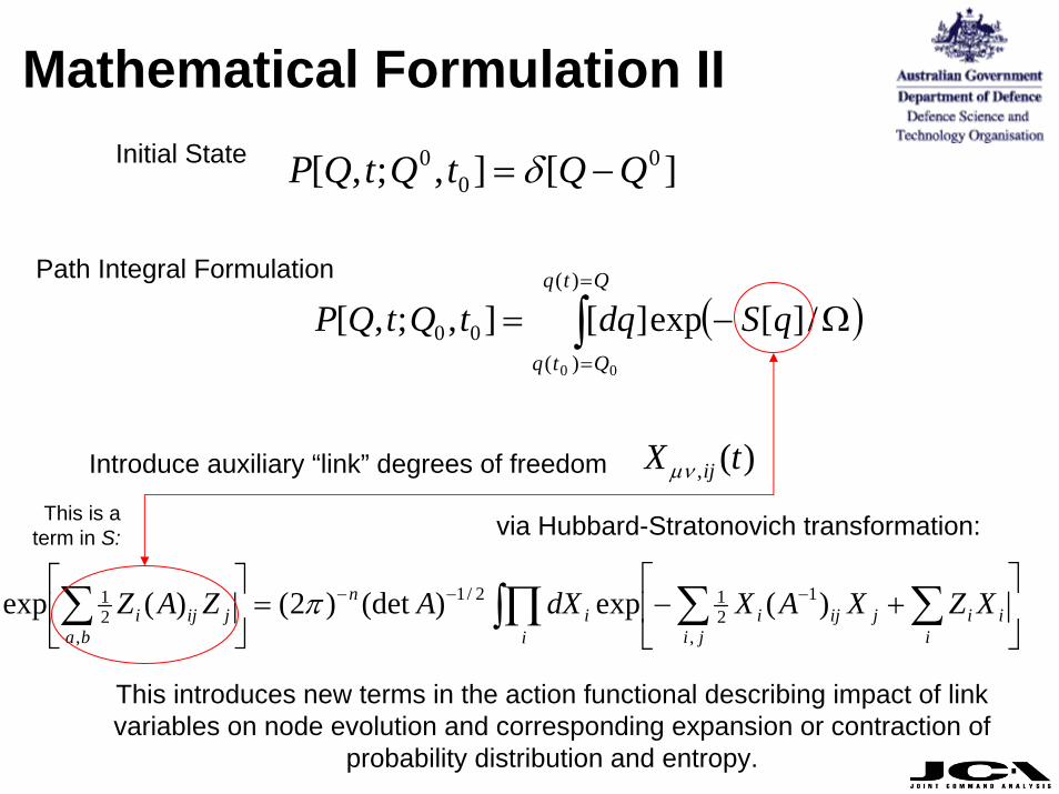
Mathematical Formulation II

][],;,[ 00

0 QQtQtQP −= δ

( )Ω−= ∫=

=

/][exp][],;,[)(

)(00

00

qSdqtQtQPQtq

Qtq

)(, tX ijμν

∫ ∑ ∑∏∑ ⎥⎦

⎤⎢⎣

⎡+−=⎥

⎦

⎤⎢⎣

⎡ −−−

ji iiijiji

ii

n

bajiji XZXAXdXAZAZ

,

1212/1

,21 )(exp)(det)2()(exp π

Path Integral Formulation

Introduce auxiliary “link” degrees of freedom

via Hubbard-Stratonovich transformation:This is a term in S:

Initial State

This introduces new terms in the action functional describing impact of link variables on node evolution and corresponding expansion or contraction of

probability distribution and entropy.

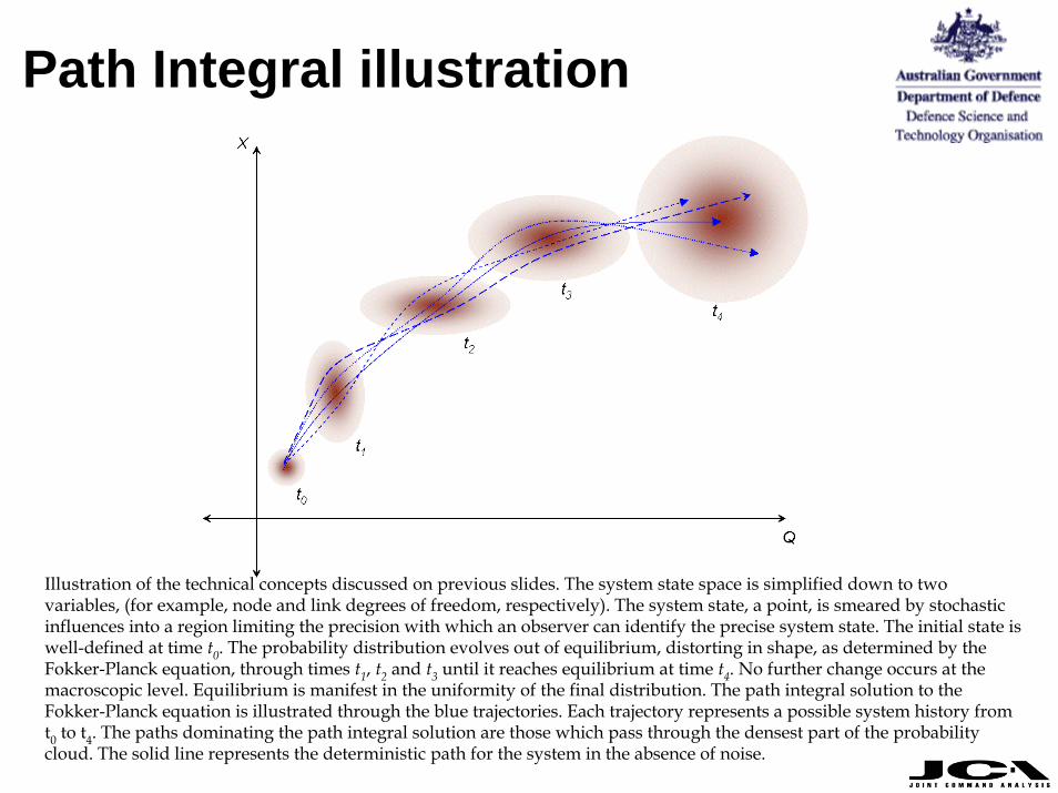
Path Integral illustration

Illustration of the technical concepts discussed on previous slides. The system state space is simplified down to two variables, (for example, node and link degrees of freedom, respectively). The system state, a point, is smeared by stochastic influences into a region limiting the precision with which an observer can identify the precise system state. The initial state is well-defined at time t0. The probability distribution evolves out of equilibrium, distorting in shape, as determined by the Fokker-Planck equation, through times t1, t2 and t3 until it reaches equilibrium at time t4. No further change occurs at the macroscopic level. Equilibrium is manifest in the uniformity of the final distribution. The path integral solution to the Fokker-Planck equation is illustrated through the blue trajectories. Each trajectory represents a possible system history from t0 to t4. The paths dominating the path integral solution are those which pass through the densest part of the probability cloud. The solid line represents the deterministic path for the system in the absence of noise.