organic matter sources, composition, and quality in …
TRANSCRIPT

ORGANIC MATTER SOURCES, COMPOSITION, AND QUALITY
IN RIVERS AND EXPERIMENTAL STREAMS
by
Julia E. Kelso
A dissertation submitted in partial fulfillment
of the requirements for the degree
of
DOCTOR OF PHILOSOPHY
in
Ecology
Approved:
______________________ ____________________
Michelle A. Baker, Ph.D. John Stark, Ph.D.
Major Professor Committee Member
______________________ ____________________
Bethany Neilson, Ph.D. Matthew Miller, Ph.D.
Committee Member Committee Member
______________________ ____________________
Zachary Aanderud, Ph.D. Laurens H. Smith, Ph.D.
Committee Member Interim Vice President for Research and
Dean of the School of Graduate Studies
UTAH STATE UNIVERSITY
Logan, Utah
2018

ii
Copyright ©Julia E. Kelso 2018
All Rights Reserved

iii
ABSTRACT
Organic Matter Sources, Composition, and Quality
in Rivers and Experimental Streams
by
Julia E. Kelso, Doctor of Philosophy
Utah State University, 2018
Major Professor: Michelle A. Baker
Department: Biology
Organic matter (OM) regulates important ecosystem functions such as nutrient
and pollutant retention, ecosystem respiration, and primary production. Through these
processes, rivers remove or slow transport of inorganic nutrients and OM that cause
eutrophication, and transform pollutants that otherwise are be transported to downstream
receiving waters. My study was motivated by research questions such as: How does OM
source and composition differ in reference versus urban watersheds with wastewater
inputs? How does OM source and quality (i.e. lability) differ across watersheds that vary
in land cover associated with human development? How much faster does labile OM
decay than semi-labile OM in rivers? What is the effect on decay rates when labile and
semi-labile OM pools of varying lability are mixed? To address these questions, I

iv
collected particulate OM (POM) and dissolved OM (DOM) in four watersheds of
Northeastern Utah. I also measured decay rates of DOM from various experimentally
derived OM sources in experimental streams. I identified and quantified the proportion of
autochthonous, terrestrial, and anthropogenic sources of OM within an entirely urban
watershed, and found significant contribution from anthropogenic sources such as a
eutrophic lake and wastewater treatment plant (WWTP) effluent. I evaluated the effects
of different land covers including urban and suburban development, crops, and other
agriculture on OM composition, and found that OM from WWTPs was distinct from
terrestrial and autochthonous OM in the same watersheds. Lastly, I measured microbial
rates of OM consumption that varied in source and quality, including high quality OM
such as algal leachates and lower quality OM such as soil and plant leachates. These
experiments revealed extremely fast DOM decay rates in experimental streams (1.7/day).
Forty percent of impaired rivers and streams in the U.S. are impaired due to
sedimentation and OM enrichment. My study identified OM sources, characterized
lability, and quantified microbial consumption of common OM sources to rivers. This
information will inform management decisions aimed at reducing organic matter loads in
rivers, such as whether to focus on reducing primary production of autochthonous
sources, or regulating terrestrial and anthropogenic OM inputs.
(212 pages)

v
PUBLIC ABSTRACT
Organic Matter Sources, Composition and Quality
in Rivers and Experimental Streams
Julia E. Kelso
Organic matter (OM) is often considered the “currency” for ecosystem processes,
such as respiration and primary production. OM in aquatic ecosystems is derived from
multiple sources, and is a complex mixture of thousands of different chemical
constituents. Therefore, it is difficult to identify all the sources of OM that enter and exit
aquatic ecosystems. As humans develop undisturbed land, the rate at which terrestrial
OM (e.g. soil and plants) and associated nutrients (e.g. nitrogen) enters rivers has
increased. Increased nutrients may lead to increased primary production from aquatic
plants and algae, potentially causing eutrophication and harmful algal blooms. In this
study, I identified and characterized different sources of OM in four watersheds of
Northeastern Utah with multiple land covers such as cities, forests, and crops. I expected
OM in watersheds with human-altered land cover would have more OM produced
instream by algae and other primary producers, than OM in less disturbed watersheds,
which typically have OM from terrestrial sources. I found that OM at river sites with high
human impact had high amounts of OM from instream primary production, but there was
also OM produced in-steam at sites with low human impact. The greatest differences in
OM across watersheds was due to wastewater treatment effluent. I also measured
microbial consumption rates of algal derived and terrestrially derived DOM in
experimental streams to quantify how much faster algal derived OM was consumed than

vi
terrestrial OM. I found algal derived OM was consumed extremely fast, so fast that
realistic measurements of its consumption in some river ecosystems may not be possible.
It is important to identify and characterize sources of OM to rivers, so watershed
managers can devise effective OM reduction plans appropriate for the constituent of
concern unique to that watershed or region. Constituents of concern associated with OM
include pathogens affiliated with manure, toxins in harmful algal blooms, metals, and
pharmaceuticals from wastewater treatment effluent. Each pollutant requires a unique
mitigation strategy and therefore the first step to pollution mitigation is source
identification.

vii
ACKNOWLEDGMENTS
We thank our funders at Utah State University, including the School of Graduate
Studies, Department of Biology, Ecology Center. This research was also supported by the
National Science Foundation (awards IIA 12-08732 and DEB 17-54216).
I would like to thank my advisor Dr. Michelle Baker for her support and
guidance. Through her mentorship I learned how to research, analyze, write, edit, and
communicate scientific questions. She also provided me and others with invaluable
interdisciplinary experience through her leadership of iUTAH. I would also like to thank
my committee members, John Stark, Beth Neilson, Matt Miller and Zach Aanderud for
their guidance and thoughtful comments.
I thank the Biology Department and Ecology Center staff for their help with field
vehicles, lab supplies, and all the details of research and graduate school they helped me
navigate. Specifically, I would like to thank Nancy Huntly for her work as director of the
Ecology Center and as a guru of transdisciplinary science. She provided myself, and
other graduate students with the opportunity to work as a science reporter for Utah Pubic
Radio, a unique experience I will draw on for the rest of my career.
I thank my family and friends for support and encouragement throughout all my
graduate studies.

viii
CONTENTS
ABSTRACT……………………………………………………………………………...iii
PUBLIC ABSTRACT…………………………………………………………………….v
ACKNOWLEDGMENTS………………………………………………………………vii
LIST OF TABLES………………………………………………………………………...x
LIST OF FIGURES……………………………………………………………………....xi
CHAPTER
I. INTRODUCTION………………………………………………………………1
Literature Cited…………………………………………………………………8
II. ORGANIC MATTER IS A MIXTURE OF TERRESTRIAL,
AUTOCHTHONOUS, AND ANTHROPOGENIC SOURCES IN AN URBAN
RIVER 13
Abstract………………………………………………………………………..13
Introduction……………………………………………………………………14
Methods…………………………………………………………………….….18
Results…………………………………………………………………………28
Discussion……………………………………………………………………..32
Literature Cited………………………………………………………………..40
Tables………………………………………………………………………….49
Figures…………………………………………………………………………52
Supplement……………………………………………………………………60
III. ORGANIC MATTER SOURCES AND COMPOSITION IN RIVERS WITH
MIXED LAND COVER…………………………………………………………65
Abstract………………………………………………………………………..65
Introduction……………………………………………………………………66
Methods………………………………………………………………………..70
Results…………………………………………………………………………82
Discussion……………………………………………………………………..87
Literature Cited………………………………………………………………..97
Tables………………………………………………………………………...107
Figures………………………………………………………………………..111
Supplement…………………………………………………………………..118

ix
IV. DOM DEMAND AND NON-ADDITIVE EFFECTS OF
AUTOCHTHONOUS AND TERRESTRIAL LEACHATES IN BIOASSAYS
AND EXPERIMENTAL STREAMS…………………………………………..130
Abstract………………………………………………………………………130
Introduction…………………………………………………………………..131
Methods………………………………………………………………………135
Results………………………………………………………………………..144
Discussion……………………………………………………………………149
Literature Cited………………………………………………………………156
Tables………………………………………………………………………...167
Figures………………………………………………………………………..170
Supplement…………………………………………………………………..175
V. CONCLUSIONS………...……………………………………….………….189
Literature Cited………………………………………………………………194
VI. CURRICULUM VITAE………...…………………………….……………196

x
LIST OF TABLES
Table Page
1-1 Fluorescence indices used to characterize and identify potential sources of DOM
in an urban river……………………………………………………………….…49
1-2 Carbon, nitrogen, and hydrogen isotope mean and standard deviation for potential
sources of Jordan River (JR) organic matter…………………………………….50
1-3 Pearson’s correlations between spectroscopic indices FI, YFI, BIX, HIX, and
SUVA and water quality metrics Chla, DOC, and TDN………………………51
2-1 Carbon, nitrogen and hydrogen isotopes values of sources used in the SIMMR
isotope mixing model………………………………………………………...…107
2-2 Watershed characteristics, water quality, and DOM spectrofluormetrics averaged
among sub-watersheds within each watershed. ………………………..............108
2-3 PARAFAC components and descriptions from references with > 97% match in
the OpenFluor database and descriptions determined for this study …………..109
2-4 PCA correlation coefficients (r) for DOM water quality metrics, PARAFAC
components, and fluorescence indices. ………………………………………...110
3-1 Single source decay rates (ktot,/d) calculated after 6, 24, and 70 hours using
equation two…………………………………………………………………….167
3-2 Descriptions of 5 components identified by PARAFAC and references that a
tucker’s congruency coefficient of 0.95 or more in the OpenFluor library…….168
3-2 Estimated decay rates (1/d) for the labile, 𝑘𝑓𝑎𝑠𝑡 and semi-labile, 𝑘𝑠𝑙𝑜𝑤 pools of
DOM in the prime-algae and prime-light experiment after 6, 24, and 70
hours…………………………………………………………………………….169

xi
LIST OF FIGURES
Figure Page
1-1 Study sites (A-I) and wastewater treatment plants (WWTP) located along the
Jordan River from Utah Lake to terminus in wetlands of the Great Salt
Lake………………………………………………………………………………52
1-2 Above the dotted line are average δ2H values of potential sources. Below the
dotted are average δ2H values of 3 size-classes of organic matter………………53
1-3 The percent feasible contributions to CPOM for 3 sources depending on
season…………………………………………………………………………….54
1-4 Percent feasible contributions to FPOM from 4 sources depending on the
month…………………………………………………………………………….55
1-5 Deuterium values of FPOM compared to deuterium of Jordan River water (top)
and FPOM δ13C values compared to δ13C of Jordan River dissolved inorganic
carbon (DIC; bottom)………………………………………………………….....56
1-6 Percent feasible contributions to DOM from 4 sources depending on the month.
Contributions were estimated using SIMMR with 2 isotope tracers…………….57
1-7 Deuterium values of DOM compared to δ2H-water (top) and δ13C-DOM
compared to δ13C of dissolved inorganic carbon (DIC; bottom)………………...58
1-8 Water quality metrics, chlorphyll a (Chla), dissolved organic carbon (DOC), and
total dissolved nitrogen (TDN), regressed against 5 spectroscopic indices,
freshness index (BIX), fluorescence index (FI), Yeomin index (YFI), humification
index (HIX) and SUVA254…………………………………………………….…59
2-1 Eight to 9 sites were sampled in each of four watersheds, the Logan River
(watershed area 1756 km2), Provo River (1810 km2), and Red Butte Creek (189
km2), a tributary of the Jordan River (2067 km2), were sampled over three
sampling efforts……………………………………………………...…………111
2-2 Principle components 1(PC1) and 2 (PC2) of a PCA with 82 DOM samples from
34 sites…………………………………………………..…………………...…112
2-3 Percent feasible contributions of 4 sources to 50 DOM samples collected in all
watersheds. Contributions were estimated with 3 isotope tracers……………...113
2-4 DOM-δ13C values compared to DIC-δ13C of river water (A), and DOM-δ2H
values compared to δ2H value of river water (B)……………………………….114

xii
2-5 Correlations between chlorophyll a (µg/L) and fluorescence indices of
microbially- derived DOM (FI, YFI), dissolved organic carbon to totoal dissolved
nitrogen ratio (DOC:TDN), and percent protein-like DOM. …………………..115
2-6 Percent feasible contributions of 4 sources to 75 FPOM samples collected in all
watersheds. Contributions were estimated with 3 isotope tracers……………...116
2-7 FPOM-δ13C values compared to DIC-δ13C of river water (A), and FPOM -δ2H
values compared to δ2H value of river water (B)……………………………….117
3-1 Eight experimental streams and 8 bottle-bioassays were used to compare decay in
bioassays versus experimental streams and test the hypothesis labile DOM would
increase the decay rate of semi-labile DOM…………………………………....170
3-2 Light streams (n=4) had significantly higher fluorescence index (FI) values than
dark streams (n=4) and all streams had higher FI values than bottles
(n=8)…………………………………………………………………………….171
3-3 Percent fluorescence contribution compared components 1 through 5 (C1, C2, C3,
C4, C5) after 1, 24 hours and 70 hours…..…………………………………..…172
3-4 Dissolved organic carbon (DOC) decay rates, bioassays, experimental streams,
and natural stream……………………………………………………………....173
3-5 Average bioavailable DOC (BDOC) was significantly greater for experimental
streams compared to bottles across all experiments except soil, which had
significantly higher BDOC than bottles, and there were no other significant
differences among experiments………………………………………………...174
INTRODUCTION
Rivers are bioreactors of organic matter (OM) that can efficiently utilize energy
from terrestrial OM inputs that would otherwise be lost to the atmosphere, or transported
to downstream waters (Fisher and Likens 1972). OM processing mediates important
ecosystem functions, such as nutrient retention and transformation, which influences
water quality in rivers and downstream lakes and estuaries. Constituents of concern that
are transformed or retained due to OM processing include trace metals (Mulholland et al.
1981, Kikuchi et al. 2017) such as mercury (Creed et al. 2018), phosphorus (Guillemette

2
et al. 2013, Larsen et al. 2015), nitrate (Taylor and Townsend 2010), and surfactants
(Sickman et al. 2007, DeBruyn and Rasmussen 2012). The balance of OM supply and
demand within a watershed regulates the net export of these constituents of concern to
downstream waters (Wollheim et al. 2018). Therefore, it is important to identify potential
sources of OM, so managers can plan to reduce and effectively limit OM supply or
possibly manipulate OM retention or transformation to increase OM demand.
The majority of particulate OM (POM) and dissolved (DOM) is presumed to
originate from terrestrial sources, and the remainder is attributed to autochthonous
sources, which are produced instream (Findlay and Sinsabaugh 2003, Findlay and Parr
2017). However, depending on OM size-class, stream order, reservoir and lake inputs,
and watershed land cover, the proportion of terrestrial versus autochthonous sources of
OM in rivers and streams (hereafter rivers) varies greatly (Wilkinson et al. 2013). Coarse
POM (CPOM is POM >1 mm) from terrestrial ecosystems is an important energy source
for consumers and higher trophic levels. CPOM is also major source of fine POM
(FPOM, POM > 0.45 µm and < 1mm) and DOM, but sources of autochthonous CPOM in
rivers is rarely reported (Wallace et al. 1982, Tank et al. 2010). FPOM has a large surface
area compared to DOM and therefore affects sorption, and nutrient and metal transport in
watersheds (Yoshimura et al. 2010, Larsen et al. 2015). While FPOM is assumed to be
primarily terrestrial, estimates of autochthonous sources of FPOM in rivers range from
less than 1% to as much as 50% (Kendall et al. 2007, Ostapenia et al. 2009, Larsen et al.
2015). Likewise, the majority of DOM is assumed to be resistant to microbial
consumption, but portions of humic-like DOM may support a significant portion of
microbial OM demand (Volk et al. 1997, Fellman et al. 2008) and the proportion of

3
humic-like OM may better predict the magnitude of microbial OM processing than more
labile OM (Amon and Benner 1996). It is hard to identify and separate autochthonous
versus terrestrial sources in the ambient DOM pool. Therefore, estimates of the
proportional contributions of each source remain unconstrained (Wilkinson et al. 2013).
As the urban footprint of metropolitan areas expands (Ng 2016), OM loads to
rivers have increased (Kaushal and Belt 2012), and the diversity of OM sources has also
increased (Stanley et al. 2012). Anthropogenic sources of POM include plastics
(McCormick et al. 2016) and wastewater treatment plant (WWTP) effluent (Sickman et
al. 2007, Gücker et al. 2011). Human land use has also altered DOM composition as a
result of impervious surfaces and agricultural landscapes which transport pollutants such
as pesticides, surfactants, and other petroleum products (Griffith et al. 2009, Sickman et
al. 2010, McElmurry et al. 2013). WWTP effluent is a source of hydrocarbons,
pharmaceuticals, and illicit drugs that WWTPs are not designed to remove during the
wastewater treatment process (Bridgeman et al. 2014). Typically anthropogenic sources
are expected to be more labile than terrestrial sources, but their relative lability compared
to autochthonous sources is not quantified. Therefore, understanding the ecological
effects of increased labile OM loads to rivers, is necessary to advance watershed
management paradigms from simple sanitation to sustainable urban landscapes (Kaushal
and Belt 2012, Parr et al. 2016).
I have introduced OM as a pool divided into unknown proportions of three
sources: terrestrial, autochthonous, and anthropogenic. The source of OM may predict
OM composition and quality (Chen and Jaffé 2014). Throughout the literature, aquatic
OM composition of terrestrial origin is described as high in aromatic and humic content,

4
which is correlated with lower proportions of amino acids and protein-like OM (Findlay
and Sinsabaugh 1999, del Giorgio and Davis 2003). Consequently, terrestrially derived
aquatic OM has a high organic carbon to organic nitrogen ratio (C:N; range of 20 to 100
in aquatic ecosystems) compared to autochthonous sources (5 to 20 C:N range; Knapik et
al. 2015, Parr et al. 2015). It is also typically composed of larger, more complex OM
constituents than autochthonous sources, which makes it less likely to be assimilated
and/or respired by microbes (Guillemette et al. 2013). Therefore, terrestrially derived OM
in rivers is characterized as a low quality carbon source for microbial consumption. In
contrast, autochthonous OM sources have greater proportions of small, simple, aliphatic,
nitrogen rich, protein-like compounds, and are classified as high quality OM (Findlay and
Sinsabaugh 1999, del Giorgio and Davis 2003, Mostofa et al. 2013). Measures of OM
composition and quality are also used as proxies of OM bioavailability, where high
quality OM is considered more bioavailable than low quality OM. Bioavailable (or labile)
OM is “preferred” by microbes, that is, rapidly consumed within hours, days, or weeks in
aquatic ecosystems versus semi-labile (or recalcitrant) OM, which is lost over months,
years, or centuries (Cory and Kaplan 2012).
Current estimates of microbial consumption or OM decay rates are highly
variable among OM sources and across aquatic ecosystems. Decay rates calculated from
natural sources of DOM in rivers, such as soil or algal leachate, range from 0.0003/d to
62.8/d (Webster and Meyer 1997, Kaplan et al. 2008). One reason for this wide range is
due to the many methods used to quantify DOM decay, including bioassays, reach-scale
tracer experiments, and ecosystem models. Bioassays, which include any closed system
incubation (e.g., dark bottles and plug-flow reactors), are commonly used to measure

5
DOM decay as bacterial respiration and/or organic carbon loss. However, most
incubations do not include a proxy for the benthic zones of lotic ecosystems (Catalán et
al. 2016, Mineau et al. 2016, Bengtsson et al. 2018), and benthic habitats are responsible
for at least half of DOM consumption (Cory and Kaplan 2012, Risse-Buhl et al. 2012,
Mineau et al. 2016). Further, results are difficult to compare across studies because
incubation times vary from days to years (Mineau et al. 2016), and are often conducted in
the dark, so bioassays do not account for effects of photodegradation, an important
abiotic driver of DOM decay (Moran and Zepp 2000, Findlay and Parr 2017). Thus to
better estimate DOM processing rates in streams, more empirical measures of
autochthonous and terrestrial OM decay that include benthic OM consumption are
needed (Mineau et al. 2016, Bengtsson et al. 2018).
The effects of increased proportions of autochthonous and/or anthropogenic OM
sources on river ecosystem function remains unclear. Increased human influence within a
watershed has increased the proportion of labile OM compared to semi-labile OM in
freshwater ecosystems (Hosen et al. 2014, Parr et al. 2015, Williams et al. 2016). It is
proposed that the smaller proportion of labile, autochthonous OM has non-additive
effects on the decay rates of semi-labile OM, such that when labile and semi-labile OM
are mixed, labile OM stimulates microbial consumption of semi-labile OM resulting in a
positive non-additive effect or “priming” effect (Bengtsson et al. 2018). Terrestrial
studies of OM non-additive effects identified positive non-additive effects over 50 years
ago (Kuzyakov et al. 2000), but results remain unclear for aquatic ecosystems (Guenet et
al. 2010, Bengtsson et al. 2018). In theory, increased anthropogenic inputs of labile OM
may increase mineralization of terrestrial OM in rivers due to non-additive effects of
6
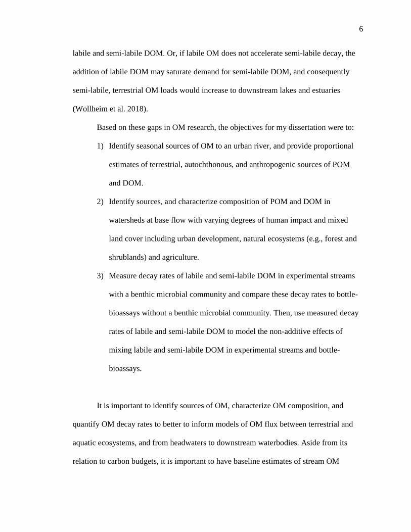
labile and semi-labile DOM. Or, if labile OM does not accelerate semi-labile decay, the
addition of labile DOM may saturate demand for semi-labile DOM, and consequently
semi-labile, terrestrial OM loads would increase to downstream lakes and estuaries
(Wollheim et al. 2018).
Based on these gaps in OM research, the objectives for my dissertation were to:
1) Identify seasonal sources of OM to an urban river, and provide proportional
estimates of terrestrial, autochthonous, and anthropogenic sources of POM
and DOM.
2) Identify sources, and characterize composition of POM and DOM in
watersheds at base flow with varying degrees of human impact and mixed
land cover including urban development, natural ecosystems (e.g., forest and
shrublands) and agriculture.
3) Measure decay rates of labile and semi-labile DOM in experimental streams
with a benthic microbial community and compare these decay rates to bottle-
bioassays without a benthic microbial community. Then, use measured decay
rates of labile and semi-labile DOM to model the non-additive effects of
mixing labile and semi-labile DOM in experimental streams and bottle-
bioassays.
It is important to identify sources of OM, characterize OM composition, and
quantify OM decay rates to better to inform models of OM flux between terrestrial and
aquatic ecosystems, and from headwaters to downstream waterbodies. Aside from its
relation to carbon budgets, it is important to have baseline estimates of stream OM

7
transformations for managers who aim to reduce OM loads, as well as to mitigate for
pathogens and contaminants associated with OM in human-altered watersheds (Edmonds
and Grimm 2011, Stanley et al. 2012). DOM can contribute to biochemical oxygen
demand, the formation of disinfection by-products, and adsorb metal contaminants
(Stanley et al. 2012, Kaushal et al. 2014). Also, OM inputs to rivers from terrestrial and
human altered landscapes needs further study at the reach, and watershed scale (as in this
study) to understand OM dynamics within larger aquatic networks of wetlands, lakes,
reservoirs, and urban or agricultural infrastructure (as in Williams et al. 2016). The study
of novel sources of DOM in anthropogenically altered landscapes is just beginning
(Stanley et al. 2012, Creed et al. 2015), and estimates of the proportional contributions of
autochthonous and terrestrial sources, as well as empirical measures of DOM decay, will
help put the ecological consequences of less studied sources of DOM in perspective. My
study provides proportional estimates of anthropogenic sources of OM in rivers and
empirical measurements of OM decay and carbon spiraling metrics that will help predict
the implications of DOM processing in streams with respect to downstream water quality.

8
Literature Cited
Amon, R. M., and R. Benner. 1996. Bacterial utilization of different size-classes of
dissolved organic matter. Limnology and Oceanography 41:41-51.
Bengtsson, M. M., K. Attermeyer, and N. Catalán. 2018. Interactive effects on organic
matter processing from soils to the ocean: are priming effects relevant in aquatic
ecosystems? Hydrobiologia 822:1-17.
Bridgeman, J., P. Gulliver, J. Roe, and A. Baker. 2014. Carbon isotopic characterisation
of dissolved organic matter during water treatment. Water Research 48:119-125.
Butman, D., S. Stackpoole, E. Stets, C. P. McDonald, D. W. Clow, and R. G. Striegl.
2016. Aquatic carbon cycling in the conterminous United States and implications for
terrestrial carbon accounting. Proceedings of the National Academy of Sciences 113:58-
63.
Catalán, N., R. Marcé, D. N. Kothawala, and L. J. Tranvik. 2016. Organic carbon
decomposition rates controlled by water retention time across inland waters. Nature
Geoscience 9:501-504.
Chen, M., and R. Jaffé. 2014. Photo-and bio-reactivity patterns of dissolved organic
matter from biomass and soil leachates and surface waters in a subtropical wetland.
Water Research 61:181-190.
Cory, R. M., and L. A. Kaplan. 2012. Biological lability of streamwater fluorescent
dissolved organic matter. Limnology and Oceanography 57:1347-1360.
Creed, I. F., A. K. Bergström, C. G. Trick, N. B. Grimm, D. O. Hessen, J. Karlsson, K. A.
Kidd, E. Kritzberg, D. M. McKnight, and E. C. Freeman. 2018. Global change‐driven
effects on dissolved organic matter composition: Implications for food webs of northern
lakes. Global Change Biology.24:3692-3714.
Creed, I. F., D. M. McKnight, B. A. Pellerin, M. B. Green, B. A. Bergamaschi, G. R.
Aiken, D. A. Burns, S. E. Findlay, J. B. Shanley, and R. G. Striegl. 2015. The river as a
chemostat: fresh perspectives on dissolved organic matter flowing down the river
continuum. Canadian Journal of Fisheries and Aquatic Sciences 72:1272-1285
DeBruyn, A. M., and J. B. Rasmussen. 2002. Quantifying assimilation of sewage‐derived
organic matter by riverine benthos. Ecological Applications 12:511-520.
del Giorgio, P., and J. Davis. 2003. Patterns in dissolved organic matter lability and
consumption across aquatic ecosystems. Pages 399-424 in S.E.G. Findlay and R.L.
Sinsabaugh (editors). Aquatic Ecosystems. Elsevier, Amsterdam.

9
Edmonds, J. W., and N. B. Grimm. 2011. Abiotic and biotic controls of organic matter
cycling in a managed stream. Journal of Geophysical Research: Biogeosciences 116.
G02015, doi:10.1029/2010JG001429.
Fellman, J. B., D. V. D’Amore, E. Hood, and R. D. Boone. 2008. Fluorescence
characteristics and biodegradability of dissolved organic matter in forest and wetland
soils from coastal temperate watersheds in southeast Alaska. Biogeochemistry 88:169-
184.
Findlay, S. E. G., and T. B. Parr. 2017. Dissolved Organic Matter. Pages 21-35 in F. R.
Hauer and G. A. Lamberti (editors). Methods in Stream Ecology. Elsevier, Amsterdam.
Findlay, S., and R. L. Sinsabaugh. 1999. Unravelling the sources and bioavailability of
dissolved organic matter in lotic aquatic ecosystems. Marine and Freshwater Research
50:781-790.
Findlay, S., and R. L. Sinsabaugh. 2003. Aquatic ecosystems: Interactivity of dissolved
organic matter. Academic Press, San Diego, California.
Fisher, S. G., and G. E. Likens. 1972. Stream ecosystem: organic energy budget.
BioScience 22:33-35.
Griffith, D. R., R. T. Barnes, and P. A. Raymond. 2009. Inputs of fossil carbon from
wastewater treatment plants to US rivers and oceans. Environmental Science and
Technology 43:5647-5651.
Gücker, B., M. Brauns, A. G. Solimini, M. Voss, N. Walz, and M. T. Pusch. 2011. Urban
stressors alter the trophic basis of secondary production in an agricultural stream.
Canadian Journal of Fisheries and Aquatic Sciences 68:74-88.
Guenet, B., M. Danger, L. Abbadie, and G. Lacroix. 2010. Priming effect: bridging the
gap between terrestrial and aquatic ecology. Ecology 91:2850-2861.
Guillemette, F., S. L. McCallister, and P. A. Giorgio. 2013. Differentiating the
degradation dynamics of algal and terrestrial carbon within complex natural dissolved
organic carbon in temperate lakes. Journal of Geophysical Research: Biogeosciences
118:963-973.
Hosen, J. D., O. T. McDonough, C. M. Febria, and M. A. Palmer. 2014. Dissolved
Organic Matter Quality and Bioavailability Changes across an Urbanization Gradient in
Headwater Streams. Environmental Science and Technology 48:7817-7824.
Kaplan, L. A., T. N. Wiegner, J. Newbold, P. H. Ostrom, and H. Gandhi. 2008.
Untangling the complex issue of dissolved organic carbon uptake: a stable isotope
approach. Freshwater Biology 53:855-864.

10
Kaushal, S. S., and K. T. Belt. 2012. The urban watershed continuum: evolving spatial
and temporal dimensions. Urban Ecosystems 15:409-435.
Kaushal, S. S., P. M. Mayer, P. G. Vidon, R. M. Smith, M. J. Pennino, T. A. Newcomer,
S. Duan, C. Welty, and K. T. Belt. 2014. Land use and climate variability amplify carbon,
nutrient, and contaminant pulses: a review with management implications. JAWRA
Journal of the American Water Resources Association 50:585-614.
Kendall, C., E. M. Elliott, and S. D. Wankel. 2007. Tracing anthropogenic inputs of
nitrogen to ecosystems.Pages 375-499 in R. Michener and K. Lajtha (editors) Stable
Isotopes in Ecology and Environmental Science, Second Edition. Blackwell Publishing,
Malden Massachusetts.
Kikuchi, T., M. Fujii, K. Terao, R. Jiwei, Y. P. Lee, and C. Yoshimura. 2017.
Correlations between aromaticity of dissolved organic matter and trace metal
concentrations in natural and effluent waters: a case study in the Sagami River Basin,
Japan. Science of The Total Environment 576:36-45.
Knapik, H. G., C. V. Fernandes, J. C. R. de Azevedo, M. M. dos Santos, P. Dall’Agnol,
and D. G. Fontane. 2015. Biodegradability of anthropogenic organic matter in polluted
rivers using fluorescence, UV, and BDOC measurements. Environmental Monitoring and
Assessment 187:104-119.
Kuzyakov, Y., J. Friedel, and K. Stahr. 2000. Review of mechanisms and quantification
of priming effects. Soil Biology and Biochemistry 32:1485-1498.
Larsen, L., J. Harvey, K. Skalak, and M. Goodman. 2015. Fluorescence‐based source
tracking of organic sediment in restored and unrestored urban streams. Limnology and
Oceanography 60:1439-1461.
McCormick, A. R., T. J. Hoellein, M. G. London, J. Hittie, J. W. Scott, and J. J. Kelly.
2016. Microplastic in surface waters of urban rivers: concentration, sources, and
associated bacterial assemblages. Ecosphere 7: e01556.
McElmurry, S. P., D. T. Long, and T. C. Voice. 2013. Stormwater dissolved organic
matter: influence of land cover and environmental factors. Environmental Science and
Technology 48:45-53.
Mineau, M. M., W. M. Wollheim, I. Buffam, S. E. Findlay, R. O. Hall, E. R. Hotchkiss,
L. E. Koenig, W. H. McDowell, and T. B. Parr. 2016. Dissolved organic carbon uptake in
streams: A review and assessment of reach‐scale measurements. Journal of Geophysical
Research: Biogeosciences 121:2019-2029.
Moran, M., and R. Zepp. 2000. UV radiation effects on microbes and microbial
processes. Microbial Ecology of the Oceans 1:201-228.

11
Mostofa, K. M., C.-q. Liu, D. Minakata, F. Wu, D. Vione, M. A. Mottaleb, T. Yoshioka,
and H. Sakugawa. 2013. Photoinduced and microbial degradation of dissolved organic
matter in natural waters. Pages 273-364 in K. Mostofa, T. Yoshioka, A. Mottableb, D.
Visone(editors) Photobiogeochemistry of Organic Matter. Springer, Berline, Heidelberg.
Mulholland, P. J., L. A. Yarbro, R. P. Sniffen, and E. J. Kuenzler. 1981. Effects of floods
on nutrient and metal concentrations in a coastal plain stream. Water Resources Research
17:758-764.
Ng, M. K. 2016. The right to healthy place-making and well-being. Planning Theory &
Practice 17:3-6.
Ostapenia, A. P., A. Parparov, and T. Berman. 2009. Lability of organic carbon in lakes
of different trophic status. Freshwater Biology 54:1312-1323.
Parr, T. B., C. S. Cronan, T. Ohno, S. E. G. Findlay, S. M. C. Smith, and K. S. Simon.
2015. Urbanization changes the composition and bioavailability of dissolved organic
matter in headwater streams. Limnology and Oceanography 60:885-900.
Parr, T. B., N. J. Smucker, C. N. Bentsen, and M. W. Neale. 2016. Potential roles of past,
present, and future urbanization characteristics in producing varied stream responses.
Freshwater Science 35:436-443.
Risse-Buhl, U., N. Trefzger, A.-G. Seifert, W. Schönborn, G. Gleixner, and K. Küsel.
2012. Tracking the autochthonous carbon transfer in stream biofilm food webs. FEMS
Microbiology Ecology 79:118-131.
Sickman, J. O., C. L. DiGiorgio, M. L. Davisson, D. M. Lucero, and B. Bergamaschi.
2010. Identifying sources of dissolved organic carbon in agriculturally dominated rivers
using radiocarbon age dating: Sacramento–San Joaquin River Basin, California.
Biogeochemistry 99:79-96.
Sickman, J., M. Zanoli, and H. Mann. 2007. Effects of urbanization on organic carbon
loads in the Sacramento River, California. Water Resources Research 43: W11422
Stanley, E. H., S. M. Powers, N. R. Lottig, I. Buffam, and J. T. Crawford. 2012.
Contemporary changes in dissolved organic carbon (DOC) in human‐dominated rivers: is
there a role for DOC management? Freshwater Biology 57:26-42.
Tank, J. L., E. J. Rosi-Marshall, N. A. Griffiths, S. A. Entrekin, and M. L. Stephen. 2010.
A review of allochthonous organic matter dynamics and metabolism in streams. Journal
of the North American Benthological Society 29:118-146.
Taylor, P. G., and A. R. Townsend. 2010. Stoichiometric control of organic carbon–
nitrate relationships from soils to the sea. Nature 464:1178-1181.

12
Volk, C. J., C. B. Volk, and L. A. Kaplan. 1997. Chemical composition of biodegradable
dissolved organic matter in streamwater. Limnology and Oceanography 42:39-44.
Wallace, J. B., D. H. Ross, and J. L. Meyer. 1982. Seston and dissolved organic carbon
dynamics in a southern Appalachian stream. Ecology 63:824-838.
Webster, J., and J. L. Meyer. 1997. Organic matter budgets for streams: a synthesis.
Journal of the North American Benthological Society 16:141-161.
Wilkinson, G. M., M. L. Pace, and J. J. Cole. 2013. Terrestrial dominance of organic
matter in north temperate lakes. Global Biogeochemical Cycles 27:43-51.
Williams, C. J., P. C. Frost, A. M. Morales‐Williams, J. H. Larson, W. B. Richardson, A.
S. Chiandet, and M. A. Xenopoulos. 2016. Human activities cause distinct dissolved
organic matter composition across freshwater ecosystems. Global Change Biology
22:613-626.
Wollheim, W., S. Bernal, D. Burns, J. Czuba, C. Driscoll, A. Hansen, R. Hensley, J.
Hosen, S. Inamdar, and S. Kaushal. 2018. River network saturation concept: factors
influencing the balance of biogeochemical supply and demand of river networks.
Biogeochemistry: doi:10.1007/s10533-018-0488-0.
Yoshimura, C., M. Fujii, T. Omura, and K. Tockner. 2010. Instream release of dissolved
organic matter from coarse and fine particulate organic matter of different origins.
Biogeochemistry 100:151-165.

13
CHAPTER II
ORGANIC MATTER IS A MIXTURE OF TERRESTRIAL, AUTOCHONOUS,
AND ANTHROPOGENIC SOURCES IN AN URBAN RIVER
Abstract: The first step to reducing organic matter (OM) loads that contribute to poor
water quality in urban watersheds is to identify the sources of OM inputs. Autochthonous
sources of OM are predicted to increase compared to terrestrial sources in urban rivers
due to higher nutrient concentrations and light availability than reference watersheds, and
anthropogenic sources of OM to urban rivers (e.g. wastewater effluent) are hard to
distinguish from other sources. Our objective was to identify sources of three size-classes
of OM to an urban river, the Jordan River, in the Salt Lake Basin, Utah, USA. Stable
isotopes of carbon, nitrogen and hydrogen were used as tracers of OM sources for
samples of coarse particulate OM (CPOM), fine particulate OM (FPOM), and dissolved
OM (DOM). Isotopes were used in a Bayesian mixing model and a graphical gradient-
based mixing model to identify autochthonous, terrestrial, and anthropogenic sources of
OM. optical properties of DOM were also used to identify the sources and composition of
DOM. We found CPOM was mostly terrestrially derived with increased autochthonous
inputs in warm months. FPOM was a mixture of terrestrially derived OM, wastewater
influenced OM, and OM from the eutrophic Utah lake. DOM was primarily from Lake-

14
DOM with increasingly significant contributions from WWTP effluent in fall. Based on
proportional estimates of autochthonous, terrestrial, lake and wastewater effluent sources
managers can better target specific sources of problematic OM loads to the Jordan River.
Additionally, baseline estimates of terrestrial versus autochthonous OM sources in an
urban river will inform developing theoretical frameworks (e.g. Urban Watershed
Continuum) that aim to understand ecosystem functions of urban watersheds.
Keywords: urban ecology, wastewater, water quality, dissolved organic matter,
particulate organic matter, natural abundance stable isotope tracer, mixing models,
deuterium
Introduction
Rivers and streams are hotspots of organic matter (OM) transport and
transformation (McClain et al. 2003, Battin et al. 2008). River metabolism is often fueled
by terrestrial inputs, and rivers have high metabolic efficiency considering their surface
area at the global scale (Fisher and Likens 1973, Duarte and Prairie 2005, Raymond et al.
2013). Recent data revealed the global surface area of streams and rivers was previously
underestimated by 40%, so they likely contribute significantly more to global carbon
cycling than previously thought (Allen and Pavelsky 2018). By storing, transporting, and
transforming OM, rivers provide important ecosystem services, such as nutrient retention
and removal that maintain water quality and ecological integrity of downstream lakes,
estuaries, and oceans. For example, river networks efficiently transform terrestrial inputs

15
into biomass that are used as energy for organisms occupying higher trophic levels
(Wallace 1997, Kominoski and Rosemond 2012). Rivers also store or mineralize
terrestrial inputs which helps to mitigate excessive nutrients (Alexander et al. 2009,
Kaushal et al. 2014) and sediment loads (Larsen and Harvey 2017) to downstream
waterbodies.
Increased urbanization has altered river geomorphology, flow regimes, and
biological community structure, potentially reducing the capacity of urban watersheds to
retain and transform OM (Meyer et al. 2001, Kominoski and Rosemond 2011, Smith and
Kaushal 2015). Hydrologic connectivity among streets, storm drains, pipe networks, and
ditches results in high drainage densities (i.e., stream length per unit watershed area) in
urban watersheds compared to natural watersheds (Baruch et al. 2018). As a result, OM
loads to urban rivers are larger than to their reference counterparts (Kaushal and Belt
2012). Excessive particulate OM (POM) loads in rivers increases nutrient concentrations
associated with POM (Larsen and Harvey 2017), thereby exacerbating symptoms of
eutrophication in urban rivers. Greater light availability and higher inorganic nutrient
concentrations in urban rivers may also increase autochthonous OM production (Bernot
et al. 2010, Smith and Kaushal 2015). A greater proportion of autochthonously derived
OM compared to terrestrially derived, is problematic because autochthonous OM sources
are more bioavailable than terrestrial sources (Kaplan and Bott 1989, del Giorgio and
Pace 2008, Parr et al. 2015). More bioavailable OM in urban watersheds compared to
reference watersheds augments microbial activity (McCallister and del Giorgio 2012)
again exacerbating symptoms of eutrophication such as increased dissolved oxygen
demand.

16
In addition to increased autochthonous sources, urban OM loads include less
studied OM sources such as storm water, impervious surface and lawn runoff (Edmonds
and Grimm 2011, Hosen et al. 2014), as well as hydrocarbons and pharmaceuticals
(Griffith et al. 2009, McElmurry et al. 2013), all of which occur at unknown quantities in
urban watersheds. Effluent from wastewater treatment plants (WWTPs) is another
possible source of labile DOM (Westerhoff and Anning 2000, Figueroa-Nieves et al.
2014) which again, would spur primary production and microbial metabolism in reaches
downstream of WWTPs. Anthropogenic OM released from wastewater treatment has
been studied for decades (Ma et al. 2001, Debryyn and Rasmussen 2002, Gücker et al.
2006), the downstream consequences of OM are often ignored (Wassenaar et al. 2010).
Also, due to the interacting effects of landuse, geomorphology, and climate it remains
difficult to quantify the downstream ecological impact of a single WWTP (Wassenaar et
al. 2010). ).
Robust estimates of autochthonous, terrestrial, and anthropogenic OM sources is
important information for watershed managers to reduce excess OM loads in impaired
urban rivers. Studies have estimated the proportion of terrestrial versus autochthonous
particulate OM (POM) in pristine freshwater ecosystems and found terrestrial sources
dominated POM (Karlsson et al. 2003, Mohamed and Taylor 2009, Solomon et al. 2011),
or was a mixture of autochthonous and terrestrial sources (Wilkinson et al 2013).
Reported proportions autochthonous dissolved OM (DOM) in lakes, ranges from 0 to
20% , and the remainder of DOM is considered terrestrial (Kritzberg et al. 2004, Bade et
al. 2007, Ostapenia et al. 2009, Wilkinson et al. 2013).

17
Proportional estimates of autochthonous, terrestrial and WWTP effluent OM
sources in rivers are limited. Autochthonous dissolved organic carbon (DOC) accounted
for upwards of 25% of total primary production per day in a nutrient-rich stream (Lyon
and Ziegler 2009), and almost 16% in a reference stream (Hotchkiss and Hall 2015).
Autochthonous sources of POM were found to increase with greater watershed area, and
represent at least half of POM in large rivers of the United States (drainage area >10,000
km2; Kendall et al 2001). In small urban streams, POM was derived from both
agricultural (15%) and WWTP (85%) sources (Gücker et al. 2011), or contributions of
autochthonous sources ranged from 20 to 50% all POM and the remainder was terrestrial
(Imberger et al. 2014). However, estimates remain uncertain because source proportions
were based on carbon and nitrogen isotope mixing models with endmember δ13C values
that overlapped.
Reference watershed DOM is dominated by terrestrial sources (Palmer et al.
2001, Hood et al. 2005, Cartwright 2010, Wilkinson et al. 2013), while urban watersheds
have an unknown proportion of laabile (Hosen et al. 2014, Imberger et al. 2014), recently
derived (Williams et al. 2016), and autochthonous DOM sources (Parr et al. 2015). Labile
DOM in urban waterways can originate from anthropogenic sources, such as runoff from
lawns and impervious surfaces, leaky septic tanks, and treated wastewater (Smith and
Kaushal 2015, Fork et al. 2018), but the proportions of anthropogenic, autochthonous,
and terrestrial sources of DOM in urban rivers remains unknown. In addition to
informing management strategies to reduce OM loads, baseline estimates of terrestrial
versus autochthonous OM sources in an urban river will inform current theoretical
frameworks, for example the urban watershed continuum that aim to extend conceptual

18
models of organic matter in reference watersheds to urban ecosystems (Vannote et al.
1980, Kaushal and Belt 2012, Kominoski and Rosemond 2012).
Our objective was to provide proportional estimates of terrestrial, autochthonous,
and anthropogenic sources of POM and DOM to an urban river, and identify how these
sources may vary across 4 watersheds within a matrix of land covers. We collected
CPOM (POM, >1mm), FPOM (POM, 1mm-0.7m and DOM throughout the year in the
Jordan River, an urban river in the Great Salt Lake Basin (Fig. 1). Optical properties of
DOM were used to identify sources and characterize DOM composition, and naturally
occurring stable isotopes of carbon, nitrogen, and hydrogen were used as tracers in
mixing models to identify OM sources. Proportional estimates of OM sources can test the
hypothesis that urbanization increases autochthonous OM in rivers, and this study
provides one of few proportional estimates of terrestrial, autochthonous, and
anthropogenic sources in a river.
Methods
Study sites and sampling regime
The Jordan River begins at Utah Lake, a shallow, eutrophic lake in the southern
portion of the Great Salt Lake Basin, and flows north 82 km where it terminates in
wetlands that connect to the Great Salt Lake. Utah Lake receives water from the Provo
River, Spanish Fork River, and American Fork River as well as wastewater effluent from
6 WWTP in these drainages (Psomas, 2009). Three WWTPs discharge effluent into the
Jordan River and are located 22, 37, and 50 km downstream from Utah Lake (Fig. 1).

19
Discharge from Utah Lake to the Jordan River is highly regulated for irrigation,
and flood control in the Salt Lake metropolitan area; average daily discharge has ranged
from 0.05 to 8.9 m3 s-1 since 1985 (Cirrus and Stantex 2009; Supplement 1). Since 1985
the river has been regulated never to exceed 9.8 cubic meters per second (CMS) as a
result of extensive flooding in 1983-1985 (Supplement 1; Hooten 2011). Depth and width
range from 0.57 m and 16 m in the first 50 km below Utah Lake to 1 m depth and 39 m
width at lower reaches (Epstein et al. 2016). The dominant substrate is gravel in the upper
reaches and fine sediments in lower reaches (Epstein et al. 2016).
Three size-classes of OM were collected at 9 sites. OM in the Jordan River is
dominated by the dissolved size-class, which makes up 94% of total annual carbon
transport, compared to 6% and 1% of FPOM and CPOM (Epstein et al. 2016). CPOM,
FPOM, and DOM were collected in April, July, September, and November of 2014, and
December of 2015 for δ13C, δ15N, and δ2H stable isotope analysis. We collected OM in
April and July to characterize OM before and after snowmelt-runoff which typically
occurs in mid-June. OM was collected in September, November, and December to
characterize OM before and after leaf senescence in October. We also collected Jordan
River water for deuterium (δ2H-water), and carbon isotopes of DIC (δ13C-DIC), at the
same time as OM (but DIC was not collected in December 2015).
Organic matter isotope sampling of CPOM, FPOM and DOM
In addition to samples collected in 2014 and 2015, CPOM samples collected from
a previous study of the Jordan River were also analyzed for δ13C, δ15N, and δ2H. Samples
from Epstein et al. (2016) were collected in February, May, July, August, and October of

20
2013. All CPOM was sampled with bedload samplers based on the Helley-Smith bedload
sampler design (Helley and Smith 1971). One-mm mesh nets were attached to the bottom
and top of a steel pole. Nets were held perpendicular to flow for 6 minutes to collect
CPOM in transit along the bottom and on the surface of the river. CPOM was then picked
from the nets and transported back to the laboratory in a cooler.
FPOM was collected as grab samples in the field with a 1-liter bottle from each
site and then transported back to the laboratory for filtering. FPOM for δ13C and δ15N
isotope analysis was filtered on 25 mm diameter glass fiber filters of 0.7 µm pore size
(Whatman GF/F, Maidstone, UK). Filters were dried at 50 °C, rewet with deionized
water, and acidified by fumigation in a desiccator with 25% HCl for 6 hours (Brodie et al.
2011). FPOM for δ2H isotope analysis was collected on 0.45 µm nylon filters (Whatman
polyamide membrane filters, Maidstone, UK) then backwashed into deionized water, and
dehydrated at 50 °C in a drying oven (Wilkinson et al. 2013). The remaining solid was
scraped from glass dishes and sent for δ 2H isotope analyses.
DOM was collected as grab samples in the field with two, 1-liter bottles at each
site and filtered in the laboratory through 0.7 µm glass fiber filters (Whatman GF/F,
Maidstone, UK). One liter was acidified to pH 2.5-3 with concentrated HCl to remove
inorganic carbon. Acidified DOM was then evaporated in 8-inch diameter glass dishes at
50 °C, residue was scraped from plates (Wilkinson et al 2013), and stored in scintillation
vials. DOM from November 2014 and December 2015 was freeze dried because several
previously collected DOM samples congealed after dehydration and were not submitted
for isotope analysis. Non-acidified DOM was also dehydrated and residue was sent for δ
2H isotope analysis.

21
Organic matter source sampling
Five endmember categories were evaluated as possible sources for each size-class
of OM: terrestrial, autochthonous, benthic organic matter (BOM), WWTP effluent and
lake sources. Except for WWTP and lake sources, 1 to 2 samples of each source were
collected from each site and dried at 50°C for stable isotope analysis. Terrestrial sources
included leaf-litter (senesced), tree leaves (not senesced), and Phragmites.
Autochthonous sources included macrophytes, biofilm, and algae. Macrophytes were cut
from large submerged aquatic vegetation anchored to the benthic zone. Biofilm was
scraped from benthic rocks, and algae were collected from green mats floating on the
water surface. Autochthonous sources were transported back to the laboratory, rinsed
with DI water, and large macroinvertebrates (>1 mm) were removed. BOM was collected
by sinking a stove-pipe 5 to 10 cm into river sediment, agitating with a meter stick, then a
100 mL sample of the sediment-water mixture was collected and stored in coolers for
transport (Wallace et al. 2006). WWTP and lake sources included OM of each-size-class
from Utah Lake (Lake-CPOM, Lake-FPOM, Lake-DOM) and WWTP effluent (WWTP-
CPOM, WWTP-FPOM, WWTP-DOM), and were collected identically to each size-class
of OM at sampling sites. Lake OM was collected directly below the Utah Lake pumping
station in a large depositional area below the pumping station (Supplement 2).
WWTP and lake sources included OM of each-size-class from Utah Lake (Lake-
CPOM, Lake-FPOM, Lake-DOM) and WWTP effluent (WWTP-CPOM, WWTP-FPOM,
WWTP-DOM), and were collected identically to each size-class of OM at sampling sites.

22
Lake OM was collected in a large depositional area below the Utah Lake pumping station
(Supplement 2). WWTP effluent was sampled directly below the effluent outfall of the
Central Valley Water Reclamation Facility on Mill Creek (Mille Creek WWTP) ca. 2 km
from the confluence of the Jordan River (Supplement 2). Effluent was only collected
from the Mill Creek WWTP because the effluent stream of the most upstream WWTP,
South Valley Water Reclamation Facility (South Valley WWTP) was difficult to
distinguish from irrigation return flows, and was very small compared to mainstem river
flow. The 3 most downstream WWTPs on the Jordan River were outside our study
domain. The South Valley and Mill Creek WWTPs are both tertiary treatment facilities
with UV disinfection, and were constructed in the early 1980s (Mill Creek 1981-1989
www.svwater.com, South Valley 1985 www.cvwrf.org). The South Valley WWTP has a
smaller capacity (25 million gallons per day) than Central Valley WWTP (75 million
gallons per day), and contributes up to half of total discharge to the Jordan River, or more
during low flow periods (Cirrus and Stantex 2009).
Stable isotope analysis
Organic matter samples for isotope analysis were prepared and analyzed using
standard methods (Hershey et al. 2017). Briefly, acidified OM samples were packed in
silver, and non-acidified samples were packed in tin capsules for stable isotope analysis.
All dried POM samples were ground in a coffee bean grinder. Samples for δ13C and δ15N
analysis were sent to the Stable Isotope Facility (SIF) at University of California Davis
on a PDZ Europa ANCA-GSL elemental analyzer interfaced to a PDZ Europa 20-20
isotope ratio mass spectrometer (Sercon Ltd., Cheshire, UK) with a long term standard

23
deviation of 0.2 ‰ for 13C and 0.3‰ 15N. Deuterium analysis was conducted at the
Colorado Plateau Stable Isotope Laboratory (CPSIL) at Northern Arizona University.
Samples were pyrolyzed to H2 gas following the procedures of Doucett et al (2007) and
analyzed with a Thermo-Finnigan TC/EA and DeltaPLUS-XL (Thermo Electron
Corporation, Bremen, Germany; precision 2‰). Samples analyzed for δ2H were
corrected for exchange of H atoms between sample and ambient water vapor using the
bench top equilibration method (Doucett et al. 2007). The δ13C of DIC was obtained by
filling helium-flushed, 12 mL exetainer vials with 1 mL of 85% phosphoric acid and 4
mL of filtered river water (Taipale and Sonninen 2009). DIC samples were analyzed
using a GasBench II system interfaced to a Delta V Plus IRMS (Thermo Scientific,
Bremen, Germany) with a long term standard deviation of 0.1 ‰. Jordan River water was
analyzed for δ2H (precision 2‰) and δ18O (precision 1‰) isotopes at the Utah State
University Stable Isotope Lab. Samples were run using a GasBench II with GC PAL
auto-sampler interfaced to a Delta V Plus IRMS (Thermo Scientific, Bremen, Germany;
precision 2‰ 2H and 1‰ 18O).
Isotope mixing model
The Stable Isotope Mixing Model in R package (SIMMR) provided a Bayesian
inference mixing model designed to estimate the proportional contribution of sources to a
mixture (Parnell and Inger 2016). SIMMR incorporates variability of end-members into
the model and estimates source contributions to a mixture regardless of the number of
isotope tracers (Parnell et al. 2013). Three isotope tracers (δ13C, δ15N, δ2H) were used to
24
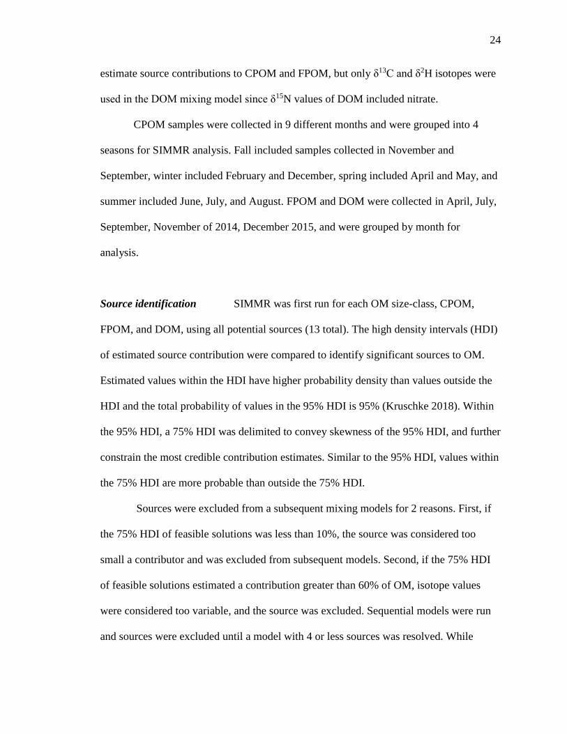
estimate source contributions to CPOM and FPOM, but only δ13C and δ2H isotopes were
used in the DOM mixing model since δ15N values of DOM included nitrate.
CPOM samples were collected in 9 different months and were grouped into 4
seasons for SIMMR analysis. Fall included samples collected in November and
September, winter included February and December, spring included April and May, and
summer included June, July, and August. FPOM and DOM were collected in April, July,
September, November of 2014, December 2015, and were grouped by month for
analysis.
Source identification SIMMR was first run for each OM size-class, CPOM,
FPOM, and DOM, using all potential sources (13 total). The high density intervals (HDI)
of estimated source contribution were compared to identify significant sources to OM.
Estimated values within the HDI have higher probability density than values outside the
HDI and the total probability of values in the 95% HDI is 95% (Kruschke 2018). Within
the 95% HDI, a 75% HDI was delimited to convey skewness of the 95% HDI, and further
constrain the most credible contribution estimates. Similar to the 95% HDI, values within
the 75% HDI are more probable than outside the 75% HDI.
Sources were excluded from a subsequent mixing models for 2 reasons. First, if
the 75% HDI of feasible solutions was less than 10%, the source was considered too
small a contributor and was excluded from subsequent models. Second, if the 75% HDI
of feasible solutions estimated a contribution greater than 60% of OM, isotope values
were considered too variable, and the source was excluded. Sequential models were run
and sources were excluded until a model with 4 or less sources was resolved. While

25
SIMMR can estimate any number of sources, we constrained our CPOM and FPOM
models to 4 sources since we had 3 isotope tracers (δ13C, δ15N and δ2H). Models for
DOM were constrained to 3 sources since we had only 2 isotope tracers for DOM (δ13C
and δ2H) because dehydrated DOM contained 15N from nitrate.
FPOM and DOM gradient-based mixing model
In addition to the Bayesian mixing model, a graphical, gradient-based mixing
model was used to partition OM sources as either terrestrial or autochthonous (Mohamed
and Taylor 2009, Rasmussen 2010, Wilkinson et al. 2013). If DOM was primarily
derived from terrestrial inputs, δ13C-DOM or δ2H-DOM would not vary systematically
with δ13C-DIC or δ2H-water, and yield a flat line with a y-intercept at the average δ13C or
δ2H terrestrial isotope values. If DOM was primarily derived from autochthonous
production, the δ13C and δ2H values would vary linearly with aqueous δ13C-DIC or δ2H-
water values (Wilkinson et al. 2013).
Water quality metrics
DOC, total dissolved nitrogen (TDN), and Chlorophyll a (Chla) were collected in
April, July, September, November, and December along with OM samples. DOC and
TDN samples were filtered through 0.7 µm glass fiber filters into 40 mL amber vials and
acidified with HCl to a pH of 2.5 for storage until carbon analysis. Acidified DOC and
TDN samples were run on a Shimadzu TOC-L analyzer via catalytic oxidation
combustion at 720 °C (DOC MDL 0.2 mg/L, TDN MDL 0.1 mg/L; Shimadzu Corp.,
Kyoto, Japan). Chla was collected on glass fiber filters, in-stream, with a drill-pump

26
(Kelso and Baker 2015), wrapped in foil, frozen, and subsequently analyzed on a Turner
handheld fluorometer (Turner Designs, Sunnyvale, CA; MDL 0.1 mg/L) following
Steinman et al (2007).
DOM spectroscopic indices
Six spectroscopic indices were calculated from excitation emission matrices
(EEMs), which were produced on a Horiba Aqualog spectrofluorometer (Horiba
Scientific, Edison, New Jersey). EEMs were collected over excitation wavelengths 248-
830 nm at 6 nm increments and over emissions 249.4-827.7 nm at 4.7 nm (8 pixel)
increments. All samples were collected in ratio mode (S/R), and run at an integration time
resulting in a maximum emission intensity of 5,000 to 50,000 counts per second,
typically 0.25 to 1 second. Samples that exceeded 0.3 absorbance units at excitation 254
nm were diluted with deionized water. All samples were corrected for inner filter effects,
Rayleigh scatter, and blank subtracted in MATLABTM (version 6.9; MathWorks, Natick,
Massachusetts) as described in Murphy et al (2013).
The fluorescence index (FI), Yeomin fluorescence index (YFI), freshness index
(BIX), humification index (HIX), peak T to peak C ratio (TC), and SUVA254 were
calculated from corrected EEMs in MATLABTM (Table 1). The FI was calculated at
excitation 370 nm as the ratio of emission intensities at 470 and 520 nm (Cory and
McKnight 2005). The YFI was calculated as the average intensity over emission 350-400
nm divided by the average intensity over emission 400-500 nm at excitation 280 nm (Heo
et al 2016). YFI was calculated in addition to the FI because the YFI can better
differentiate fluorophore precursor materials than the FI, and it is less sensitive to

27
concentration-dependent effects (Heo et al. 2016). For example, the YFI has a wide index
range for fulvic, humic, aminosugar-like, and protein-like fluorophores (0.30-6.41). In
contrast, the FI has a narrower index range (0.82-2.14), and cannot distinguish between
protein-like and aminosugar-like standards (Heo et al. 2016). The β:α index (BIX), also
called the freshness index, was calculated as the intensity at excitation 380 nm divided by
the max intensity between emission 420-435 nm, where higher values represent more
recently derived DOM (Parlanti et al. 2000). The HIX was calculated at excitation 254
nm as the area under emission 435-480 divided by the area under emission 300-450 nm +
435-480 nm; higher HIX values represent more humic-like material (Zsolnay et al. 1999).
The TC index is the ratio of maximum fluorescence in the peak T region (protein-like)
versus peak C region (humic-like) with higher values representing more protein-like
DOM, which are also associated with WWTP effluent (Baker 2001). TC was calculated
as the ratio of maximum fluorescence at excitation 275/em350 nm to max intensity
within excitation 320-340nm/emission 410-430 nm (Gabor et al. 2014). Last, SUVA254,
an indicator of aromaticity, was calculated from DOM absorbance at 254 nm normalized
by DOC concentration (Weishaar et al. 2003). Nitrate and iron interferences with
fluorescence and absorbance indices were ruled out following Weishaar et al. (2003)
given iron concentrations were < 1 mg/L (Jordan River maximum 0.08 mg/L) and nitrate
concentrations were < 40 mg/L (maximum 20.4 mg/L TDN this study, maximum NO2-
+NO3-N 8 mg/L, Epstein et al. 2016).
Spectroscopic indices were correlated to water quality metrics with all months
combined. Correlations were conducted with the GGally package in R (Schloerke et al.

28
2014). Correlations were considered significant when correlation coefficients were
greater than 0.35 (Rohlf and Sokal 1995).
Results
Source isotope values
Deuterium was the only isotope that sufficiently separated autochthonous and
terrestrial sources (Fig. 2). Biofilm, algae, and macrophytes had the most negative δ2H
values (-222.6 ‰, standard deviation (sd) 35.9; Table 2). WWTP-FPOM, WWTP-DOM,
and Lake-DOM had the most positive δ2H values (Fig. 2). All other sources had average
δ2H values between -150 to -200‰. Variation in δ13C and δ2H values of autochthonous
sources (mean coefficient of variation, 0.22 δ13C ‰ and 0.12 δ2H ‰) was greater than
terrestrial sources (mean coefficient of variation, 0.04 δ13C ‰ and 0.07 δ2H ‰). Average
δ15N for all sources were between 5 ‰ and 10 ‰ except for WWTP-DOM which had
more positive values (29.4 δ15N ‰) because it included enriched WWTP-derived nitrate.
Average δ13C values from autochthonous sources overlapped the range of terrestrial δ13C
values, again highlighting that only δ2H isotopes may be able to differentiate between
autochthonous and terrestrial sources (Table 2).
Carbon and hydrogen isotope values were similar between leaf-litter and tree leaf
sources (Table 2). Therefore if SIMMR did not distinguish sources depending on the
δ15N isotope value of an OM size-class, as was the case with FPOM and DOM, these leaf
sources were averaged together and modeled as one terrestrial source
(Litter+TreeLeaves). However, because leaf-litter had depleted δ15N values (mean 3.9, sd

29
2.4‰) compared to living tree leaves (mean 6.9, sd 3.5‰), SIMMR was able to
distinguish litter and tree leaves as different sources to CPOM (see below).
CPOM
Bayesian model Three possible sources of CPOM were identified: biofilms,
macrophytes and leaf-litter. Algae, BOM, living tree leaves, Lake-FPOM, Lake-DOM,
WWTP-FPOM, and WWTP-FPOM were excluded from the model because proportional
estimates were <10%, and all other excluded sources had proportional estimates with
variability >60% (Supplement 3.1). Leaf-litter always represented the greatest feasible
proportion of CPOM, except in summer when leaf-litter and macrophyte contributions
were roughly equal (Fig. 3). Macrophytes were the second most likely source of CPOM;
contributions ranged from 4 to 38% in fall, increased in winter and spring, and greatest
feasible proportions were in summer (15-64%). Biofilm was the least likely source of
CPOM with higher contributions estimated in spring (3-34%), and summer (5 to 26%)
compared to fall and winter.
FPOM
Bayesian model Four potential sources of FPOM were identified by SIMMR,
including Lake-FPOM, WWTP-FPOM, Litter+TreeLeavess and BOM. Autochthonous
sources, Phragmites, and WWTP-DOM were excluded from the model because
proportional estimates were <10%, and all other excluded sources had proportional
estimates with variability >60% (Supplement 3.1). BOM and Lake-FPOM had higher
feasible proportions in July and September, than November and December, ranging from

30
9 to 82% in July and 8 to 58% in September (Fig. 4). Litter+TreeLeaves increased from
July to December with median percent contributions of 12 % in July and 18% in
December. WWTP-FPOM was greatest in September and November, and ranged from 16
to 69% over both months. In sum, terrestrial sources of FPOM increased in autumn, with
possible autochthonous contributions from Lake-FPOM in July and September, and from
WWTP-FPOM in September and November. April was not included because there was
not enough particulate for analysis of δ2H.
Graphical gradient model If FPOM was derived from 100% autochthonous sources,
we expected δ2H-FPOM and δ13C-FPOM values to have a positive relationship with δ2H-
water and δ13C-DIC. Lake samples were excluded from δ13C gradient models because
Lake DIC-δ13C values were extremely high compared to all other OM (Fig. 5).There
were no significant linear relationships between δ2H-FPOM and δ2H-water within
months, or among all months combined (Fig. 5 top, Supplement 4). FPOM δ2H values
averaged -166.3 ‰ (sd 13.6) which was similar to average terrestrial sources (-163.8 ‰,
sd 11.5). WWTP FPOM had δ2H-FPOM values (mean -140‰, sd 16.2) that were more
positive than terrestrial δ2H values (Fig. 5 top). Several FPOM samples from July had
lower δ2H values than terrestrial sources, suggesting autochthonous contributions to
FPOM in July. November δ13C-FPOM and δ13C-DIC values had a positive relationship (r
= 0.44, p = 0.04); all other months were not significantly correlated. The results of both
models indicated FPOM was primarily terrestrial in November and December with
possible autochthonous contributions from Lake-FPOM and BOM in July, and increased
contributions from WWTP-FPOM in September and November.

31
DOM
Bayesian model DOM was composed of 3 sources, Lake-DOM, WWTP-DOM and
Litter+TreeLeaves. SIMMR predicted average terrestrial contributions of 16%, and
WWTP-DOM contributions averaged 27% throughout the year. Lake-DOM was always
the most likely DOM source and averaged 57% throughout the year. Autochthonous
sources, Phragmites, BOM, Lake-CPOM, Lake-FPOM, and WWTP-CPOM were
excluded from the model because proportional estimates were <10%, and WWTP-FPOM
was excluded because proportional estimates of WWTP-FPOM were too variable (75%
HDI >60%; Supplement 3.1). Lake-DOM was the primary source of Jordan River DOM,
with median contributions that ranged from 48 to 70 % throughout the year (Fig. 6).
WWTP-DOM was the second most likely source of DOM, with median values ranging
from 20 to 33% in all months. Litter+Tree leaves contributions were similar among July,
November, and December (mean 11%, sd 7), but were greater in September (mean 29%,
sd 10).
Graphical-gradient model If DOM was derived from 100 % terrestrial sources, we
expected no relationship between δ2H-DOM and δ13C-DOM versus δ2H-water and δ13C-
DIC, and a flat line near terrestrial values. All δ2H-DOM values were more positive
(mean –103.6 ‰, sd 19.3) than average δ2H values of terrestrial sources (Fig.7), and there
were no significant linear relationships between δ2H-DOM and δ2H-water (Supplement
4). There were positive relationships between δ13C-DOM and δ13C-DIC in April and
November (Fig. 7), but these relationships were dependent on WWTP-DOM values,

32
which had more positive δ13C-DOM values than other sites in each month. Both models
indicated Lake-DOM was a major source of DOM in the Jordan River, and DOM was
neither autochthonous nor terrestrial but had major contributions from WWTPs
throughout the year.
Relationships between spectroscopic indices and water quality
Correlations of spectroscopic indices and water quality metrics indicated DOM
was microbial derived but not necessarily autochthonously derived. Chla was negatively
correlated with FI (r = -0.43) and YFI (r = -0.48) values (Table 3, Fig. 8). This negative
relationship was due to higher Chla concentrations and low FI/YFI values in July,
compared to higher FI/YFI values and low Chla in November and December (Table 3,
Fig. 8). DOC was positively correlated with FI (r = 0.51) and YFI (r = 0.45) values and
negatively correlated with HIX (r= -0.28) and SUVA (r = -0.42; Table 3, Fig. 8).
Therefore, samples with high DOC concentrations were more microbial-derived, and less
aromatic, than samples with low DOC concentrations. SUVA values were also
significantly higher in September than all other months, indicating increased aromatic
content of DOM in September (Supplement 5). TC values were too variable to interpret
as biologically significant, likely due to highly correlated Peak T and Peak C.
Discussion
The POM sources we identified were consistent with previous OM studies in
urban watersheds, which found POM was a mixture of sources including periphyton,

33
leaves, and grass (Newcomer et al. 2012), WWTP effluent (Gücker et al. 2011), as well
as algae and macrophytes (Imberger et al. 2013). In the Jordan River, CPOM was
primarily terrestrial with a greater proportion of autochthonous sources in warm months.
Macrophytes and biofilms contributed the most to CPOM in summer, an average of 40%
and 18%, respectively (Fig. 3). FPOM was at least 12% terrestrially-derived throughout
the year and increased to an average of 56% in December (Fig. 4). SIMMR predicted 3
other sources of FPOM including WWTP-FPOM, Lake-FPOM, and BOM. WWTP-
FPOM contributions were greatest in fall due to less dilution from Lake-FPOM after
irrigation season (Supplement 1). Water is released from Utah Lake during spring to late
summer to regulate spring runoff and meet irrigation requirements and then water
released from Utah lake decreases in fall (Cirrus and Stantec 2009). Similarly, a recent
study of the Jordan River found Utah Lake accounted for roughly 50% of discharge in the
upstream reach in summer, versus 20% in fall, and WWTP effluent was consistently
between 30 and 50% throughout the year (personal communication, Jennifer Follstad
Shah, University of Utah).
Consistent with lake discharge to the river, Lake-FPOM contributions were
greatest in July, and we assumed Lake-FPOM was mostly autochthonous for two reasons.
First, Chla concentrations were highest at all sites in July and reached up to 30 µg/L in
Utah Lake (Fig. 8). Second, δ2H-FPOM values were lower than average terrestrial δ2H
values in July indicative of autochthonous sources which have lower δ2H values than
terrestrial sources (Fig. 5; Doucett et al. 2007).
We found the majority of DOM was neither autochthonous nor terrestrial
throughout the year. Median terrestrial contributions from Litter+TreeLeaves averaged

34
15% for all 4 months, and the highest average contributions were in September (29%, sd
12.5; Fig. 6). Fluorescence indices and δ2H isotope values indicated the remainder of
DOM was microbial-derived, but not from autochthonous sources. High FI/YFI values
(>2) indicated microbial derived DOM (Heo et al. 2016, Ateia et al. 2017), and high
FI/YFI were associated with WWTP river locations, and were negatively correlated to
Chla (Fig. 8). The FI was designed to distinguish between autochthonous and terrestrial
endmembers, based on fulvic acids isolated from a black water river in Georgia (the
Suawannee, FI = 1.2), and a productive lake in Antarctica (Pony Lake, FI = 1.5; Cory and
McKnight 2005, Cory et al. 2010). The FI has since been broadly applied to bulk DOM
samples across ecosystem types with typical values ranging between 1.1 and 1.8 (Jaffé et
al. 2008). However, at high DOC concentrations the relationship between fluorescence
intensity and DOC concentration is not linear and therefore when comparing samples
over a wide range of concentrations the change in FI may not represent the degree of
change in DOM composition (Korak et al. 2014). FI values above 2 have been attributed
to WWTP-sourced DOM specifically (Dong and Rosario-Ortiz 2012, Hansen et al. 2016,
Ateia et al. 2017).
In addition to high FI and YFI, all δ2H-DOM and most δ13C-DOM values were
more positive than average terrestrial isotope values collected in this study (Fig. 7), as),
as well as more positive than terrestrial values in a similar study of Midwestern lakes
(Wilkinson et al. 2013). In the literature, terrestrial sources range from -124 to -161 δ2H
‰ which is much more negative than Jordan River δ2H-DOM values (Doucett et al.
2007, Collins et al. 2016). We concluded DOM was primarily microbial derived from

35
WWTP effluent sources and Utah Lake, or a combination of the 2 considering Utah Lake
receives effluent from 6 WWTPs.
We cannot know the source or mechanism for enriched δ2H-DOM values, but we
propose 3 possible explanations. First, assuming WWTP OM is primarily derived from
humans, δ2H-DOM would reflect human δ2H values. Human hair directly correlates with
local tap water δ2H values (Ehleringer et al. 2008) which range from -131.9 to -93.6‰ in
the Salt Lake Valley (Jameel et al. 2016). Additionally, one other study reported a δ2H-
WWTP value of -52 ‰ (Spies et al. 1989), but this value was produced prior to
development of standard methods that account for exchangeable hydrogen of OM and
may not be comparable to other δ2H ‰ values (Wassenaar and Hobson 2000). Second,
Lake-DOM was the primary source of DOM which also had enriched δ2H-DOM values (-
86.1‰, sd 18.2) compared to all other sources (Table 2). While we expected Utah Lake
DOM to have more negative δ2H values due to autochthonous production of DOM, Utah
Lake had enriched δ2H-DOM values due to evaporative enrichment of δ2H-water in Utah
Lake (Jameel et al. 2016). While water was retained in Utah Lake, microorganisms likely
used enriched lake water for photosynthesis which would enrich microbial-derived δ2H-
DOM. However, Utah Lake also receives effluent from 6 WWTPs, and therefore, WWTP
as a source of DOM in Utah Lake cannot be discounted. Third, since δ2H-DOM samples
were not acidified, DOM may have included bicarbonate, which might make δ2H-DOM
more positive. We believe bicarbonate contamination was minimal because δ13C-DOM
samples were acidified, and also had more positive δ13C values than other sources.
Additionally, FPOM δ2H would have contained bicarbonate contamination as well, but
36
FPOM δ2H values were in the same range as terrestrial values suggesting minimal
bicarbonate contamination even though samples were not acidified.
This study highlights a gap in evolving urban aquatic ecosystem frameworks
which have yet to incorporate the role of higher order streams/rivers (e.g. > 1000 km2), as
well as the effects of reservoirs or inlet/outlet lakes within urban watersheds on OM
source and quality. The Urban Stream Syndrome (Walsh et al. 2005) characterized urban
stream hydrology of engineered headwaters and stream networks as flashy, which is the
opposite of urban rivers like the Jordan River which are highly regulated, and largely
sourced as a lake outlet. Likewise the Urban Watershed Continuum is based on low order
streams of the Baltimore Long Term Ecological Research (Kaushal and Belt 2012, Smith
and Kaushal 2015) and calls for further research in OM dynamics from human influenced
headwaters, to rivers, and estuaries to better mitigate the effects of urban pollution that
result in hypoxic dead zones, as observed in the Chesapeake Bay (Baskin et al. 2002) or
in the case of the Jordan River, pollution of the Great Salt Lake (Naftz et al. 2008). There
are many examples of studies of OM quality and quantity in large, urban rivers with
WWTP inputs, including foundational work in the Santa Cruz and Gila Rivers of
Phoenix, AZ (Westerhoff and Anning 2000, Edmonds and Grimm 2011), Hudson River,
NY (Findlay 2005, del Giorgio and Pace 2008, Caraco et al. 2010) and Sacramento River,
CA (Sickman et al. 2007), but the results of these studies have yet to be incorporated into
a larger framework that links headwaters to estuaries in human impacted watersheds
(Kaushal and Belt 2012). Evidence from studies on the Jordan River indicate reaches
directly downstream of the dam-controlled lake are metabolically autotrophic, and lower
reaches are heterotrophic because of fine sediments and turbidity that limit light

37
penetration in the water column (Epstein et al. 2016). Our findings suggest heterotrophic
activity in lower reaches may also be spurred by labile WWTP effluent inputs.
Specifically, this study informs the total maximum daily load (TMDL) plan
developed by the state of Utah. The plan identifies OM as the cause of low dissolved
oxygen concentrations in the lower section of the Jordan (Cirrus and Stantec 2009). The
TMDL identified 35 possible sources of POM to the Jordan River, primarily from storm
water runoff and tributaries. We narrowed primary sources of POM and DOM throughout
the year, and found sources from Utah Lake and WWTPs contributed greatly to DOM,
the largest pool of OM (Epstein et al. 2016). Dilution from non-WWTP water is a
common mechanism to mitigate adverse effects of excessive nutrient and OM loads from
(Edmonds and Grimm 2011, Gücker et al. 2011), and this study can help water
companies and managers to effectively plan and allocate water released from Utah Lake
throughout the year to mitigate excessive OM loads of concern (Cirrus and Stantex
2009). Since Utah Lake was the primary DOM source to the Jordan River, reducing OM
loads or improving water quality in the river would also require improved water quality
of Utah Lake.
OM load reduction and regulation begins with source identification, and therefore,
this study informs future management of urban river water quality. Excessive OM loads
may increase the cost of wastewater treatment and make treatment less effective (Chow
et al. 2005). For example, algal-derived DOM reduces WWTP effectiveness through
increased coagulant demand and membrane fouling (Nyguen et al. 2005, Henderson et al.
2008). Likewise, microbial and algal-derived DOM is produced and persists throughout
the treatment process, and upon chlorination may form hazardous disinfection-products

38
by (Nyguen et. al. 2005, Bridgeman et al. 2014). To prevent increased WWTP costs and
energy use in the future managers could consider strategies that may reduce
autochthonous sources in the Jordan River such as reducing autochthonous inputs from
Utah Lake, decreasing inorganic nutrient inputs at base flow, and/or mitigating inorganic
nutrient pulses during storms. Increased habitat heterogeneity through construction of
riffle and pool sequences along the Jordan River could increase retention and microbial
processing of OM. However, this strategy would have to balance the benefits of increased
OM retention with flood hazards, and construction of new depositional areas that may
increase primary production in oxic habitats or methanogenesis in anoxic habitats. This
study can inform efforts to effectively manage OM loads in urban ecosystems, as well as
inform future studies that aim to understand the ecological consequences of
anthropogenic OM inputs to rivers and streams.
Acknowledgements
We would like to thank Dave Epstein, Joe Crawford, and Hayden Campbell for
help in the field and laboratory. This manuscript was improved by thoughtful comments
from Zach Aanderud, Matt Miller, Beth Neilson, and John Stark. We thank Melanie
Caron at the Colorado Plateau Stable Isotope Facility and staff at the U.C. Davis Stable
Isotope Facility for isotope analysis guidance. This research was supported in part by
NSF EPSCoR cooperative agreement IIA- 1208732 awarded to Utah State University, as
part of the State of Utah EPSCoR Research Infrastructure Improvement Award.
Additional support was provided by the South Valley Water Reclamation Facility and

39
Utah Department of Environmental Quality. Any opinions, findings, and conclusions or
recommendations expressed are those of the author(s) and do not necessarily reflect the
views of the National Science Foundation, South Valley Water Reclamation Facility, or
the State of Utah.

40
Literature Cited
Alexander, R. B., J. K. Böhlke, E. W. Boyer, M. B. David, J. W. Harvey, P. J.
Mulholland, S. P. Seitzinger, C. R. Tobias, C. Tonitto, and W. M. Wollheim. 2009.
Dynamic modeling of nitrogen losses in river networks unravels the coupled effects of
hydrological and biogeochemical processes. Biogeochemistry 93:91-116.
Allen, G. H., and T. M. Pavelsky. 2018. Global extent of rivers and streams. Science
361:585-588.
Ateia, M., O. G. Apul, Y. Shimizu, A. Muflihah, C. Yoshimura, and T. Karanfil. 2017.
Elucidating adsorptive fractions of natural organic matter on carbon nanotubes.
Environmental Science and Technology 51:7101-7110.
Bade, D. L., S. R. Carpenter, J. J. Cole, M. L. Pace, E. Kritzberg, M. C. Van de Bogert,
R. M. Cory, and D. M. McKnight. 2007. Sources and fates of dissolved organic carbon in
lakes as determined by whole-lake carbon isotope additions. Biogeochemistry 84:115-
129.
Baker, A. 2001. Fluorescence excitation− emission matrix characterization of some
sewage-impacted rivers. Environmental Science and Technology 35:948-953.
Baruch, E. M., K. A. Voss, J. R. Blaszczak, J. Delesantro, D. L. Urban, and E. S.
Bernhardt. 2018. Not all pavements lead to streams: variation in impervious surface
connectivity affects urban stream ecosystems. Freshwater Science 37:673-684.
Baskin, R. L., K. M. Waddell, S. A. Thiros, E. M. Giddings, H. K. Hadley, D. W.
Stephens, and S. J. Gerner 2002. Water-Quality assessment of the Great Salt Lake basins,
Utah, Idaho, and Wyoming—Environmental setting and study design. U.S. Geological
Survey. Salt Lake City, UT.
Battin, T. J., L. A. Kaplan, S. Findlay, C. S. Hopkinson, E. Marti, A. I. Packman, J. D.
Newbold, and F. Sabater. 2008. Biophysical controls on organic carbon fluxes in fluvial
networks. Nature Geoscience 1:95-100.
Bernot, M. J., D. J. Sobota, R. O. Hall, P. J. Mulholland, W. K. Dodds, J. R. Webster, J.
L. Tank, L. R. Ashkenas, L. W. Cooper, and C. N. Dahm. 2010. Inter‐regional
comparison of land‐use effects on stream metabolism. Freshwater Biology 55:1874-1890.
Bridgeman, J., P. Gulliver, J. Roe, and A. Baker. 2014. Carbon isotopic characterisation
of dissolved organic matter during water treatment. Water Research 48:119-125.
Brodie, C. R., M. J. Leng, J. S. Casford, C. P. Kendrick, J. M. Lloyd, Z. Yongqiang, and
M. I. Bird. 2011. Evidence for bias in C and N concentrations and δ13C composition of
terrestrial and aquatic organic materials due to pre-analysis acid preparation methods.
Chemical Geology 282:67-83.

41
Caraco, N., J. E. Bauer, J. J. Cole, S. Petsch, and P. Raymond. 2010. Millennial-aged
organic carbon subsidies to a modern river food web. Ecology 91:2385-2393.
Cartwright, I. 2010. The origins and behaviour of carbon in a major semi-arid river, the
Murray River, Australia, as constrained by carbon isotopes and hydrochemistry. Applied
Geochemistry 25:1734-1745.
Chow, A. T., S. Gao, and R. A. Dahlgren. 2005. Physical and chemical fractionation of
dissolved organic matter and trihalomethane precursors: A review. Journal of Water
Supply: Research and Technology-AQUA 54:475-507.
Cirrus Ecological Solutions, LC, and Stantec Consulting Inc. 2009. Jordan River total
maximum daily load water quality study – Phase 1. Utah Department of Environmental
Quality. Salt Lake City, UT.
Collins, S. M., T. J. Kohler, S. A. Thomas, W. W. Fetzer, and A. S. Flecker. 2016. The
importance of terrestrial subsidies in stream food webs varies along a stream size
gradient. Oikos 125:674-685.
Cory, R. M., and D. M. McKnight. 2005. Fluorescence spectroscopy reveals ubiquitous
presence of oxidized and reduced quinones in dissolved organic matter. Environmental
Science and Technology 39:8142-814.
Cory, R. M., M. P. Miller, D. M. McKnight, J. J. Guerard, and P. L. Miller. 2010. Effect
of instrument-specific response on the analysis of fulvic acid fluorescence spectra.
Limnology and Oceanography: Methods 8:67-78.
DeBruyn, A. M., and J. B. Rasmussen. 2002. Quantifying assimilation of sewage‐derived
organic matter by riverine benthos. Ecological Applications 12:511-520.
del Giorgio, P. A., and M. L. Pace. 2008. Relative independence of organic carbon
transport and processing in a large temperate river: The Hudson River as both pipe and
reactor. Limnology and Oceanography 53:185-197.
Doucett, R. R., J. C. Marks, D. W. Blinn, M. Caron, and B. A. Hungate. 2007. Measuring
terrestrial subsidies to aquatic food webs using stable isotopes of hydrogen. Ecology
88:1587-1592.
Dong, M. M., and F. L. Rosario-Ortiz. 2012. Photochemical formation of hydroxyl
radical from effluent organic matter. Environmental Science and Technology 46:3788-
3794.
Duarte, C. M., and Y. T. Prairie. 2005. Prevalence of heterotrophy and atmospheric CO2
emissions from aquatic ecosystems. Ecosystems 8:862-870.

42
Edmonds, J. W., and N. B. Grimm. 2011. Abiotic and biotic controls of organic matter
cycling in a managed stream. Journal of Geophysical Research: Biogeosciences
116:G02015.
Ehleringer, J. R., G. J. Bowen, L. A. Chesson, A. G. West, D. W. Podlesak, and T. E.
Cerling. 2008. Hydrogen and oxygen isotope ratios in human hair are related to
geography. Proceedings of the National Academy of Sciences 105:2788-2793.
Epstein, D. M., J. E. Kelso, and M. A. Baker. 2016. Beyond the urban stream syndrome:
organic matter budget for diagnostics and restoration of an impaired urban river. Urban
Ecosystems 19:1041-1061.
Figueroa-Nieves, D., W. H. McDowell, J. D. Potter, G. Martínez, and J. R. Ortiz-Zayas.
2014. Effects of sewage effluents on water quality in tropical streams. Journal of
Environmental Quality 43:2053-2063.
Findlay, S. E. 2005. Increased carbon transport in the Hudson River: unexpected
consequence of nitrogen deposition? Frontiers in Ecology and the Environment 3:133-
137.
Fisher, S. G., and G. E. Likens. 1973. Energy flow in Bear Brook, New Hampshire: an
integrative approach to stream ecosystem metabolism. Ecological Monographs 43:421-
439.
Fork, M. L., J. R. Blaszczak, J. M. Delesantro, and J. B. Heffernan. 2018. Engineered
headwaters can act as sources of dissolved organic matter and nitrogen to urban stream
networks. Limnology and Oceanography Letters 3:215-224.
Gabor, R. S., A. Baker, D. M. McKnight, and M. P. Miller. 2014. Fluorescence indices
and their interpretation. Pages 303:338 in P.G. Coble, J. Lead, A. Baker, D.M. Reynolds,
R.G.M. Spencer (editors) Aquatic Organic Matter Fluorescence. Cambridge University
Press, New York, New York.
Griffith, D. R., R. T. Barnes, and P. A. Raymond. 2009. Inputs of fossil carbon from
wastewater treatment plants to US rivers and oceans. Environmental Science and
Technology 43:5647-5651.
Gücker, B., M. Brauns, and M. T. Pusch. 2006. Effects of wastewater treatment plant
discharge on ecosystem structure and function of lowland streams. Journal of the North
American Benthological Society 25:313-329.
Gücker, B., M. Brauns, A. G. Solimini, M. Voss, N. Walz, and M. T. Pusch. 2011. Urban
stressors alter the trophic basis of secondary production in an agricultural stream.
Canadian Journal of Fisheries and Aquatic Sciences 68:74-88.

43
Hansen, A. M., T. E. C. Kraus, B. A. Pellerin, J. A. Fleck, B. D. Downing, and B. A.
Bergamaschi. 2016. Optical properties of dissolved organic matter (DOM): Effects of
biological and photolytic degradation. Limnology and Oceanography 61:1015-1032.
Helley, E. J., and W. Smith. 1971. Development and calibration of a pressure-difference
bedload sampler. U.S. Geological Survey Open-File Report 73-108.
Henderson, R. K., A. Baker, S. A. Parsons, and B. Jefferson. 2008. Characterisation of
algogenic organic matter extracted from cyanobacteria, green algae and diatoms. Water
Research 42:3435-3445.
Henderson, R. K., A. Baker, K. Murphy, A. Hambly, R. Stuetz, and S. Khan. 2009.
Fluorescence as a potential monitoring tool for recycled water systems: a review. Water
Research 43:863-881.
Heo, J., Y. Yoon, D.-H. Kim, H. Lee, D. Lee, and N. Her. 2016. A new fluorescence
index with a fluorescence excitation-emission matrix for dissolved organic matter (DOM)
characterization. Desalination and Water Treatment 57:20270-20282.
Hershey, A.H., R. M. Northington, J.C. Finlay, and B.J. Peterson. 2017. Stable isotopes
in stream food webs. Pages 3-20 in F. R. Hauer and G. A. Lamberti (editors). Methods in
Stream Ecology. Elsevier, Amsterdam.
Hood, E., M. W. Williams, and D. M. McKnight. 2005. Sources of dissolved organic
matter (DOM) in a Rocky Mountain stream using chemical fractionation and stable
isotopes. Biogeochemistry 74:231-255.
Hooten, L.H. 2011 Utah Lake and The Jordan River Flood Control. Acessed, April 20,
2013 http://www.slcdocs.com/utilities/NewsEvents/news2011/news6282011.htm.
Hosen, J. D., O. T. McDonough, C. M. Febria, and M. A. Palmer. 2014. Dissolved
organic matter quality and bioavailability changes across an urbanization gradient in
headwater streams. Environmental Science and Technology 48:7817-7824.
Hotchkiss, E. R., and R. O. Hall. 2015. Whole-stream 13C tracer addition reveals distinct
fates of newly fixed carbon. Ecology 96:403-416.
Imberger, S. J., P. L. Cook, M. R. Grace, and R. M. Thompson. 2014. Tracing carbon
sources in small urbanising streams: catchment‐scale stormwater drainage overwhelms
the effects of reach‐scale riparian vegetation. Freshwater Biology 59:168-186.
Jaffé, R., D. McKnight, N. Maie, R. Cory, W. McDowell, and J. Campbell. 2008. Spatial
and temporal variations in DOM composition in ecosystems: The importance of long-
term monitoring of optical properties. Journal of Geophysical Research 113:G04032.

44
Jameel, Y., S. Brewer, S. P. Good, B. J. Tipple, J. R. Ehleringer, and G. J. Bowen. 2016.
Tap water isotope ratios reflect urban water system structure and dynamics across a
semiarid metropolitan area. Water Resources Research 52:5891-5910.
Kaplan, L. A., and T. L. Bott. 1989. Diel fluctuations in bacterial activity on streambed
substrata during vernal algal blooms: effects of temperature, water chemistry, and habitat.
Limnology and Oceanography 34:718-733.
Karlsson, J., A. Jonsson, M. Meili, and M. Jansson. 2003. Control of zooplankton
dependence on allochthonous organic carbon in humic and clear-water lakes in northern
Sweden. Limnology and Oceanography 48:269-276.
Kaushal, S. S., and K. T. Belt. 2012. The urban watershed continuum: evolving spatial
and temporal dimensions. Urban Ecosystems 15:409-435.
Kaushal, S. S., P. M. Mayer, P. G. Vidon, R. M. Smith, M. J. Pennino, T. A. Newcomer,
S. Duan, C. Welty, and K. T. Belt. 2014. Land use and climate variability amplify carbon,
nutrient, and contaminant pulses: a review with management implications. JAWRA
Journal of the American Water Resources Association 50:585-614.
Kelso, J. E., and M. A. Baker. 2015. Filtering with a drill pump: an efficient method to
collect suspended sediment. Journal of the American Water Resources Association. 52:1-
7.
Kendall, C., S. R. Silva, and V. J. Kelly. 2001. Carbon and nitrogen isotopic
compositions of particulate organic matter in four large river systems across the United
States. Hydrological Processes 15:1301-1346.
Korak, J. A., A. D. Dotson, R. S. Summers, and F. L. Rosario-Ortiz. 2014. Critical
analysis of commonly used fluorescence metrics to characterize dissolved organic matter.
Water Research 49:327-338.
Kominoski, J. S., and A. D. Rosemond. 2012. Conservation from the bottom up:
forecasting effects of global change on dynamics of organic matter and management
needs for river networks. Freshwater Science 31:51-68.
Kritzberg, E. S., J. J. Cole, M. L. Pace, W. Granéli, and D. L. Bade. 2004. Autochthonous
versus allochthonous carbon sources of bacteria: Results from whole‐lake 13C addition
experiments. Limnology and Oceanography 49:588-596.
Kruschke, J. K. 2018. Rejecting or accepting parameter values in Bayesian estimation.
Advances in Methods and Practices in Psychological Science 1:270-280.
Larsen, L., and J. Harvey. 2017. Disrupted carbon cycling in restored and unrestored
urban streams: Critical timescales and controls. Limnology and Oceanography 62.

45
Lyon, D. R., and S. E. Ziegler. 2009. Carbon cycling within epilithic biofilm
communities across a nutrient gradient of headwater streams. Limnology and
Oceanography 54:439-449.
Ma, H., H. E. Allen, and Y. Yin. 2001. Characterization of isolated fractions of dissolved
organic matter from natural waters and a wastewater effluent. Water research 35:985-
996.
McCallister, S. L., and P. A. del Giorgio. 2012. Evidence for the respiration of ancient
terrestrial organic C in northern temperate lakes and streams. Proceedings of the National
Academy of Sciences 109:16963-16968.
McClain, M. E., E. W. Boyer, C. L. Dent, S. E. Gergel, N. B. Grimm, P. M. Groffman, S.
C. Hart, J. W. Harvey, C. A. Johnston, and E. Mayorga. 2003. Biogeochemical hot spots
and hot moments at the interface of terrestrial and aquatic ecosystems. Ecosystems 6:301-
312.
McElmurry, S. P., D. T. Long, and T. C. Voice. 2013. Stormwater dissolved organic
matter: influence of land cover and environmental factors. Environmental Science and
Technology 48:45-53.
Meyer, J. L., M. J. Paul, and W. K. Taulbee. 2005. Stream ecosystem function in
urbanizing landscapes. Journal of the North American Benthological Society 24:602-612.
Mohamed, N. M., and W. D. Taylor. 2009. Relative contribution of autochthonous and
allochthonous carbon to limnetic zooplankton: A new cross-system approach. Archiv für
Hydrobiologie 175:113-124.
Murphy, K. R., C. A. Stedmon, D. Graeber, and R. Bro. 2013. Fluorescence spectroscopy
and multi-way techniques. PARAFAC. Analytical Methods 5:6557-6566.
Naftz, D., C. Angeroth, T. Kenney, B. Waddell, N. Darnall, S. Silva, C. Perschon, and J.
Whitehead. 2008. Anthropogenic influences on the input and biogeochemical cycling of
nutrients and mercury in Great Salt Lake, Utah, USA. Applied Geochemistry 23:1731-
1744.
Newcomer, T. A., S. S. Kaushal, P. M. Mayer, A. R. Shields, E. A. Canuel, P. M.
Groffman, and A. J. Gold. 2012. Influence of natural and novel organic carbon sources
on denitrification in forest, degraded urban, and restored streams. Ecological Monographs
82:449-466.
Nguyen, M.-L., P. Westerhoff, L. Baker, Q. Hu, M. Esparza-Soto, and M. Sommerfeld.
2005. Characteristics and reactivity of algae-produced dissolved organic carbon. Journal
of Environmental Engineering 131:1574-1582.

46
Ostapenia, A. P., A. Parparov, and T. Berman. 2009. Lability of organic carbon in lakes
of different trophic status. Freshwater Biology 54:1312-1323.
Palmer, S. M., D. Hope, M. F. Billett, J. J. Dawson, and C. L. Bryant. 2001. Sources of
organic and inorganic carbon in a headwater stream: evidence from carbon isotope
studies. Biogeochemistry 52:321-338.
Parlanti, E., K. Wörz, L. Geoffroy, and M. Lamotte. 2000. Dissolved organic matter
fluorescence spectroscopy as a tool to estimate biological activity in a coastal zone
submitted to anthropogenic inputs. Organic Geochemistry 31:1765-1781.
Parnell, A., and R. Inger 2016. Stable isotope mixing models in R with SIMMR. R
package version 0.3. R Project for Statistical Computing, Vienna Austria. (Available
from: https://cran.r-project.org/web/packages/simmr/vignettes/simmr.html)
Parnell, A. C., D. L. Phillips, S. Bearhop, B. X. Semmens, E. J. Ward, J. W. Moore, A. L.
Jackson, J. Grey, D. J. Kelly, and R. Inger. 2013. Bayesian stable isotope mixing models.
Environmetrics 24:387-399.
Parr, T. B., C. S. Cronan, T. Ohno, S. E. G. Findlay, S. M. C. Smith, and K. S. Simon.
2015. Urbanization changes the composition and bioavailability of dissolved organic
matter in headwater streams. Limnology and Oceanography 60:885-900.
Psomas Consulting. 2009. Utah Lake TMDL: pollutant loading assessment & designated
beneficial use impairment assessment. Utah Division of Water Quality.
Rasmussen, J. B. 2010. Estimating terrestrial contribution to stream invertebrates and
periphyton using a gradient‐based mixing model for δ13C. Journal of Animal Ecology
79:393-402.
Raymond, P. A., J. Hartmann, R. Lauerwald, S. Sobek, C. McDonald, M. Hoover, D.
Butman, R. Striegl, E. Mayorga, and C. Humborg. 2013. Global carbon dioxide
emissions from inland waters. Nature 503:355-359.
Revelle, W. R. 2017. psych: Procedures for personality and psychological research.
Rouder, J. N., R. D. Morey, P. L. Speckman, and J. M. Province. 2012. Default Bayes
factors for ANOVA designs. Journal of Mathematical Psychology 56:356-374.
Rohlf, F. J., and R. R. Sokal. 1995. Statistical tables. Freeman & Comp, San Francisco,
CA.
Schloerke, B., J. Crowley, D. Cook, H. Hofmann, H. Wickham, F. Briatte, M. Marbach,
and E. Thoen. 2014. GGally: Extension to ggplot2. R package version 1.4. R Project for
Statistical Computing, Vienna, Austria. (Available from: https://cran.r-
project.org/web/packages/GGally/index.html)

47
Sickman, J., M. Zanoli, and H. Mann. 2007. Effects of urbanization on organic carbon
loads in the Sacramento River, California. Water Resources Research 43.
Smith, R. M., and S. S. Kaushal. 2015. Carbon cycle of an urban watershed: exports,
sources, and metabolism. Biogeochemistry 126:173-195.
Smith, R. M., and S. S. Kaushal. 2015. Carbon cycle of an urban watershed: exports,
sources, and metabolism. Biogeochemistry 126:173-195.
Solomon, C. T., S. R. Carpenter, M. K. Clayton, J. J. Cole, J. J. Coloso, M. L. Pace, M. J.
Vander Zanden, and B. C. Weidel. 2011. Terrestrial, benthic, and pelagic resource use in
lakes: results from a three-isotope Bayesian mixing model. Ecology 92:1115-1125.
Spies, R. B., H. Kruger, R. Ireland, and D. W. Rice Jr. 1989. Stable isotope ratios and
contaminant concentrations in a sewage-distorted food web. Marine Ecology Progress
Series 54:157-170.
Steinman, A. D., G. A. Lamberti, and P. R. Leavitt. 2007. Biomass and Pigments of
Benthic Algae. Pages 357-379 in F. R. Hauer and G. A. Lamberti (editors). Methods in
Stream Ecology. Elsevier, Amsterdam.
Taipale, S. J., and E. Sonninen. 2009. The influence of preservation method and time on
the δ13C value of dissolved inorganic carbon in water samples. Rapid Communications in
Mass Spectrometry 23:2507-2510.
Vannote, R. L., G. W. Minshall, K. W. Cummins, J. R. Sedell, and C. E. Cushing. 1980.
The river continuum concept. Canadian Journal of Fisheries and Aquatic Sciences
37:130-137.
Wallace, J. B., J. R. Webster, and W. R. Woodall. 1977. The role of filter feeders in
flowing waters. Archiv für Hydrobiologie 79:506-S32.
Wallace, J. B., J. J. Hutchens, and J. W. Grubaugh. 2006. Transport and Storage of
FPOM. Pages 249-271 in F. R. Hauer and G. A. Lamberti (editors). Methods in Stream
Ecology. Elsevier, Amsterdam.
Walsh, C. J., A. H. Roy, J. W. Feminella, P. D. Cottingham, P. M. Groffman, and R. P.
Morgan II. 2005. The urban stream syndrome: current knowledge and the search for a
cure. Journal of the North American Benthological Society 24:706-723.
Wassenaar, L. I., and K. A. Hobson. 2000. Improved method for determining the stable-
hydrogen isotopic composition (δD) of complex organic materials of environmental
interest. Environmental Science and Technology 34:2354-2360.
Wassenaar, L., J. Venkiteswaran, S. Schiff, and G. Koehler. 2010. Aquatic community
metabolism response to municipal effluent inputs in rivers quantified using diel δ 18O

48
values of dissolved oxygen. Canadian Journal of Fisheries and Aquatic Sciences 67:1232-
1246.
Weishaar, J. L., G. R. Aiken, B. A. Bergamaschi, M. S. Fram, R. Fujii, and K. Mopper.
2003. Evaluation of specific ultraviolet absorbance as an indicator of the chemical
composition and reactivity of dissolved organic carbon. Environmental Science and
Technology 37:4702-4708.
Westerhoff, P., and D. Anning. 2000. Concentrations and characteristics of organic
carbon in surface water in Arizona: influence of urbanization. Journal of Hydrology
236:202-222.
Wilkinson, G. M., M. L. Pace, and J. J. Cole. 2013. Terrestrial dominance of organic
matter in north temperate lakes. Global Biogeochemical Cycles 27:43-51.
Williams, C. J., P. C. Frost, A. M. Morales‐Williams, J. H. Larson, W. B. Richardson, A.
S. Chiandet, and M. A. Xenopoulos. 2016. Human activities cause distinct dissolved
organic matter composition across freshwater ecosystems. Global Change Biology
22:613-626.
Zsolnay, A., E. Baigar, M. Jimenez, B. Steinweg, and F. Saccomandi. 1999.
Differentiating with fluorescence spectroscopy the sources of dissolved organic matter in
soils subjected to drying. Chemosphere 38:45-50.

49
Tables
Table 1. Fluorescence indices used to characterize and identify potential sources of DOM in the Jordan River, Salt Lake City,
Utah. High and low values represent index ranges expected in developed watershedsa and do not encompass all possible values
of each index.
Index Abbreviation high values
indicate:
Low values
indicate: Reference
Fluorescence index FI 1.8 microbial
derived 1.2
terrestrial
derived
Cory and
McKnight 2005
Yeomin
fluorescence index YFI 2-7
aminosugar and
protein-like 0-2 humic-like
Heo et al.
2016
Freshness index
(β:α) BIX 0.7-0.9 recently derived 0.3-0.5
less recently
derived
Parlanti et al.
2000
Humification index HIX variable
lower H/C
ratios
indicative of
humification
variable
lower degree
of
humification
Zsolnay et al.
1999
Peak T to Peak C
ratio TC 1
wastewater-like,
high
biochemical
oxygen demand
0
low
biochemical
oxygen
demand
Baker 2001
Specific UV
absorbance
at 254 nm
SUVA 3-6
greater
proportion
aromatic content
0-3
lower
proportion
aromatic
content
Weishaar et al.
2003
a See Hosen et al. 2014, Parr et al. 2015, Williams et al. 2016

50
Table 2. Mean isotope values and standard deviation for potential sources of Jordan River
organic matter (OM) including autochhtonous and terrestrial sources, OM from Utah
Lake and WWTP effluent, and average isotope values for each size-class of OM. Stable
Isototpe Analsysis In R (SIMMR) was conducted on all size-classes, and gradient-based
mixing models were conducted for FPOM and DOM. Nitrogen isotope values were not
used as a tracer in the SIMMR DOM model due to nitrate contamination of DOM.
Sources n δ13C ‰ δ15N ‰ δ2H ‰
Average Autochthonous -25.5 ± 5.7 8.7 ± 4.9 -222.6 ± 27.7
Macrophytes 24 -26.5 ± 4.6 10.4 ± 5.4 -198.0 ± 21.1
Biofilm 30 -22.4 ± 5.6 9.3 ± 3.8 -244.2 ± 29.4
Algae 10 -29.6 ± 7.1 6.3 ± 5.4 -255.6 ± 32.6
Average Terrestrial -27.2 ± 1.2 5.8 ± 3.1 -163.8 ± 11.5
Senesced leaf-litter 11 -27.8 ± 0.6 3.9 ± 2.4 -165.8 ± 10.0
Living tree leaves 17 -28.5 ± 1.4 6.9 ± 3.5 -159.4 ± 9.1
Phragmites 11 -28.4 ± 1.7 9.6 ± 3.5 -170.4 ± 15.4
BOM 21 -22.9 ± 4.8 5.1 ± 2.1 -202.3 ± 24.0
Lake-CPOM 2 -25.6 ± 0.5 7.4 ± 1.8 -164.4 ± 5.3
Lake-FPOM 5 -19.1 ± 6.1 6.8 ± 1.8 -186.7 ± 19.3
Lake-DOM 6 -25.9 ± 2.0 5.0 ± 3.9 -86.1 ± 18.2
WWTP-CPOM 5 -25.6 ± 1.7 10.4 ± 3.2 -182.4 ± 12.4
WWTP-FPOM 5 -23.9 ± 0.5 8.5 ± 1.2 -140.4 ± 16.2
WWTP-DOM 5 -23.5 ± 3.5 29.4 ± 12.4a -121.5 ± 15.2
Jordan River OM CPOM 49 -27.0 ± 1.4 8.6 ± 2.5 -182.2 ± 28.3
FPOM 28 -22.1 ± 2.9 7.2 ± 1.6 -166.8 ± 13.6
DOM 30 -25.4 ± 1.7 25.1 ± 15.4 a -117.2 ± 19.3
DIC and water River-DIC 34 -9.4 ± 0.9 Lake-DIC 8 -2.7 ± 0.9 WWTP-DIC 8 -8.3 ± 0.6 River-water 49 -98.0 ± 15.9
Lake-water 8 -77.6 ± 30.9
WWTP-water 11 -111.7 ± 9.2
a - DOM nitrogen isotope values include nitrate and were not included in the Bayesian
mixing models

51
Table 3. Pearson’s correlations between spectroscopic indices FI, YFI, BIX, HIX, and
SUVA and water quality metrics Chla, DOC, and TDN. Correlations were run between
indices and water quality metrics for all months combined (see Fig. 8).
Chla µg/L DOC mg/L TDN mg/L
BIX 0.05 -0.2 -0.43
HIX 0.15 -0.28 -0.29
FI -0.43 0.51 0.86
YFI -0.48 0.45 0.63
SUVA -0.11 -0.42 -0.12

52
Figures
Figure 1. Study sites (A-I) and wastewater treatment plant (WWTP) located along the
Jordan River from Utah Lake to terminus in wetlands of the Great Salt Lake. Light grey
represents urban land-cover.

53
Figure 2. Above the dotted line are average δ2H values of potential sources. Below the
dotted are average δ2H values of 3 size-classes of organic matter. Dots represent the
means and whiskers are 1 standard deviation. Autochthonous sources were the average of
macrophytes, biofilms and algae. Terrestrial sources were the average of senesced leaf-
litter, living tree-leaves and Phragmites (Table 2).

54
Figure 3. The percent feasible contributions of 3 sources to CPOM depending on season.
Contributions were estimated using SIMMR with 3 isotope tracers, δ13C, δ15N, and δ2H.
Boxes represent the 75% high density interval; whiskers represent the 95% high density
interval.

55
Figure 4. Percent feasible contributions to FPOM from 4 sources depending on the
month. Contributions were estimated using SIMMR with 3 isotope tracers, δ13C, δ15N,
and δ2H. Boxes represent the median and 75% high density interval; whiskers represent
the 95% high density interval.

56
Figure 5. Deuterium values of FPOM compared to δ2H-water (top) and δ13C-FPOM
compared to δ13C of dissolved inorganic carbon (DIC; bottom). The dashed lines and
grey areas represent the average deuterium and carbon isotope values of terrestrial
sources collected in this study (see Table 2). Grey circles represent FPOM collected from
WWTP effluent, black circles are FPOM collected from Utah Lake and open circles are
all other sites.

57
Figure 6. Percent feasible contributions to DOM from 4 sources depending on the month
collected. Contributions were estimated using SIMMR with 2 isotope tracers, δ13C and
δ2H. Boxes represent the median and 75% high density interval; whiskers represent the
95% high density interval.

58
Figure 7. Deuterium values of DOM compared to δ2H-water (top) and δ13C-DOM
compared to δ13C of dissolved inorganic carbon (DIC; bottom). The dashed lines and
grey area represent the average δ2H and δ13C values of terrestrial sources collected in this
study (see Table 2). Grey circles represent FPOM collected from WWTP effluent, black
circles are FPOM collected from Utah Lake and open circles are all other sites.

59
Figure 8. Water quality metrics, chlorphyll a (Chla µg/L), dissolved organic carbon
(DOC mg/L), and total dissolved nitrogen (TDN mg/L), correlated to 5 fluorescence
indices,freshness index (BIX), flourescence index (FI), Yeomin index (YFI),
humification index (HIX) and SUVA.

60
Supplement
Supplement 1. Top: Mean daily discharge for the Jordan River (JR) at site H (Figure 1) in
2014 and 2015 (gage 10171000). A 10-day moving average was calculated for each year
of daily discharge. Upside-down triangles (4) represent sampling dates in 2014 and the
triangle represents the sampling date in 2015. Bottom: Flow duration curve since 1985
until sampling period. After 1985 Utah Lake was regulated so the JR would never exceed
9.8 m3/s (Hooten 2011). Discharge exceedance probability represents the percent of time
discharge is predicted to be met or exceeded over the period of record.

61
Supplement 2. Locations where Lake and WWTP OM endmembers were collected. Top:
just below the Jordan River pumping station Lake samples were collected by wading into
the thalweg. Bottom: WWTP OM collection site at Central Valley Water Reclamation
Facility on Mill Creek just below effluent outfall. Samples were collected by floating into
the thalweg on a one-man raft.

62
Supplement 3. Table of sources that were included and excluded for each SIMMR model.
If a source had a 75% HDI that was <10% it was excluded, and if the 75% HDI had a
range >60% the source was excluded.
CPOM FPOM DOM
Macrophytes Included <10% <10%
Biofilm Included <10% <10%
Algae <10% <10% <10%
Senesced leaf-litter Included Included Included
Living tree leaves 0-80% Included Included
Phragmites 0-60% <10% <10%
BOM <10% Included <10%
Lake-CPOM 0-60% 0-60% <10%
Lake-FPOM <10% Included <10%
Lake-DOM <10% 0-100% Included
WWTP-CPOM 0-100% 0-60% <10%
WWTP-FPOM <10% Included 0-60%
WWTP-DOM <10% <10% Included

63
Supplement 4. Table of linear regressions results for graphical analysis of gradient based
mixing models of FPOM (top) and DOM (bottom). Analyses were run for each month
and for all months combined.
δ2H-FPOM vs δ2H-Water δ13C-FPOM vs δ13C-DIC
Month n slope r p n slope R p
Apr - - - - 7 -0.33 0.16 0.2
Jul 8 -0.29 0.35 0.07 8 -0.29 -0.14 0.72
Sep 7 -0.59 0.627 0.02 7 -0.69 -0.19 0.95
Nov 8 -0.17 -0.08 0.51 8 0.45 0.44 0.04
Dec 6 0.45 -0.15 0.58 - - - -
All Months 29 -0.29 0.05 0.12 30 0.17 0.19 0.01
δ2H-DOM vs δ2H-Water δ13C-DOM vs δ13C-DIC
Month n slope r p n slope r p
Apr - - - - 6 1.18 0.55 0.05
Jul 8 0.13 -0.07 0.49 8 0.21 -0.03 0.41
Sep 8 0.82 0.09 0.24 7 0.03 -0.16 0.71
Nov 6 0.38 0.41 0.09 7 0.31 0.49 0.05
Dec 7 -0.12 0.03 0.32 - - - -
All Months 29 -0.19 0.05 0.13 28 -0.02 0.04 0.82

64
Supplement 5. Boxplots of water quality metrics, Chlorophyll a (Chla, µg/L), dissolved
organic carbon (DOC, mg/L), and total dissolved nitrogen (TDN, mg/L) and index values
for Fluorescence Index (FI), Yeomin Flourescence Index (YFI), Biological index (BIX),
PeakT to PeakC ratio (TC), humification index (HIX) and SUVA grouped by month.

65
CHAPTER III
ORGANIC MATTER SOURCES AND COMPOSITION IN
RIVERS WITH MIXED LAND COVER
Abstract: As human dominated landscapes have expanded, the diversity of organic
matter (OM) sources to rivers has increased and knowledge of the composition and
quality of these sources is lacking. The source and quality of OM regulate ecosystem
functions that affect material retention and transport within a watershed. Aquatic OM is a
complex mixture of thousands of organic molecules, which makes OM source difficult to
identify within a matrix of land covers. We collected fine particulate OM (FPOM) and
dissolved OM (DOM), in 4 watersheds of north-east Utah with a mixture of urban, forest,
and agricultural land cover. We used the natural abundance of 13C, 15N, and 2H isotopes
in mixing models to quantify the proportion of terrestrial, autochthonous, and
anthropogenic OM. We also used the fluorescence and absorbance properties of DOM to
characterize OM composition as microbial versus humic derived, and bioavailability
based on percent protein-like DOM. Percent land cover within a watershed did not
explain differences in proportional sources of OM among sites. The greatest differences
in OM composition was due to the influence of wastewater treatment plants (WWTP) at a
subset of the urban sites. FPOM and DOM were primarily derived from terrestrial
sources, except at sites influenced by wastewater which had significant contributions

66
from WWTP derived OM. In addition, sites influenced by WWTPs had more
homogenous DOM that consistently had ~ 35% protein-like DOM. All other sites had
much more percent protein-like DOM. Further study is needed to understand landscape
drivers of DOM bioavailability and composition, and studies in watersheds with WWTPs
should incorporate direct measures of WWTP OM when comparing OM composition
across land covers.
Keywords: dissolved organic matter, fine particulate organic matter, mixing models,
land cover, water quality, urban ecology, PARAFAC, wastewater
Introduction
Organic matter (OM) across aquatic and terrestrial ecosystems is a complex
mixture of thousands of organic molecules and exists in in every compartment of the
hydrologic cycle. OM source, composition, and bioavailability to microbes (i.e. quality)
are directly linked. Identification of OM sources is a challenge, due to the multiple
origins of OM in rivers, including inputs from terrestrial and anthropogenic sources, as
well as OM produced in situ through primary production. OM source identification is
helpful so watershed managers can understand the origins of excessive OM loads, and
infer its bioavailability. OM produced in-stream, autochthonous OM, is considered more
bioavailable (i.e. labile) to microbes compared to terrestrial sources because microbial
activity associated with photosynthesis produces exudates of simple, low molecular
weight compounds that are easy for microbes to consume (Guillemette et al. 2013, Wyatt

67
et al. 2014). Autochthonously derived OM has proportionally more nitrogen rich
compounds (e.g. amino acids, DNA), than terrestrial sources and therefore is also
considered high quality OM that is preferentially consumed in nutrient limited conditions
(Knapik et al. 2014, Guenet et al. 2010).
The quality of OM in rivers regulates functions such as decomposition and
nutrient assimilation that affect material retention and transport within watersheds.
Excessive labile OM and inorganic nutrient loads to rivers can saturate microbial demand
for high quality OM, thereby reducing transformation and retention of semi-labile OM
(Edmonds and Grimm 2011, Wollheim et al. 2018). Consequently, OM and associated
nutrients and pathogens are transported downstream to lakes and estuaries causing
pollution and eutrophication which pose significant public health risks, and increase the
cost of drinking water treatment (Chow et al. 2005, Shutova et al. 2014). Therefore, it is
important to identify the sources and composition of OM in rivers to inform management
strategies aimed at improving water quality in both rivers and downstream water bodies.
With increased urbanization and other land-use changes, the diversity of
anthropogenic OM inputs to rivers has increased (Stanley et al. 2012, Fork et al. 2018)
adding to the complexity, and difficulty, of characterizing OM sources and composition.
For example, conversion of wetlands to agriculture was thought to destabilize fossil-aged
soil OM, which contributed large OM loads to the Sacramento River (Sickman et al.
2007). However, the same indicators of fossil soil OM (radiocarbon values) may also
signify the contribution of anthropogenic sources of petroleum products from wastewater
effluent, urban runoff, or pesticides (Sickman et al. 2010, Butman et al. 2015). Other
anthropogenic sources of OM include detergents, pharmaceuticals (Kolpin et al. 2002),

68
microplastics (McCormick et al. 2016), leaky sewage pipes and septic tanks (Kaushal and
Belt 2012), grass clippings, and pet waste (Mallin et al. 2006). Many of these
anthropogenic sources are discharged from wastewater treatment plants (WWTPs), which
are not equipped to remove pharmaceuticals and petroleum products (Bridgeman et al.
2014). The ‘ecological footprint’ of wastewater effluent on downstream organic matter
processing and production, and effects at higher trophic levels needs further study in
rivers to understand the consequences of anthropogenic sources of OM to downstream
lakes and estuaries (Wassenaar et al. 2010, Figueroa-Nieves et al. 2014, Hansen et al.
2016).
Numerous studies have aimed to describe OM sources and quality in watersheds
with different land covers and gradients of human impact. Fine particulate OM (FPOM),
OM between 0.45 and 1000 µm (Hutchens et al. 2017), was more autochthonously
derived in agricultural and urban watersheds compared to watersheds with less human
influence (Newcomer et al. 2012, Imberger et al. 2014). Dissolved OM (< 0.45 µm) in
urban watersheds was more bioavailable (Hosen et al. 2014,), autochthonous (Petrone et
al. 2011, Parr et al. 2015), and had greater proportions of hydrophobic/petroleum OM
(McElmurry et al. 2013), than DOM in non-urban watersheds. Agricultural land use was
associated with less complex, more microbial-derived OM compared to forest land cover
(Wilson and Xenopoulos 2008, Williams et al. 2010). But, only one study has
successfully distinguished DOM associated with urban versus agricultural land cover,
and differences were dependent on the scale of comparison, and type of waterbody (e.g.
lake vs. river, Williams et al. 2016).

69
The ability to link OM sources and composition to OM bioavailability is an
exciting frontier in OM research. Traditional methods to assess bioavailability with
bioassays that measure dissolved organic carbon (DOC) decay, biochemical oxygen
demand (BOD), or bioavailable dissolved organic carbon (BDOC), are informative but
labor intensive. Development of spectrofluorometers that can rapidly analyze DOM
samples and produce 3-dimensional fluorescence excitation-emission matrices (EEMs)
has driven advancements in characterizing DOM character and function (Shutova et al.
2014). EEMs produce peaks over a range of excitation and emission wavelengths, and
depending on peak location, DOM can be characterized as humic-like or protein-like
(Coble 1996). The percent protein-like DOM in a sample has been directly correlated to
DOC decay rate (Parr et al. 2015), BOD (Baker and Inverarity 2004), and BDOC
(Fellman et al. 2008, Balcarczyk et al. 2009, Petrone et al. 2011, Hosen et al. 2014),
making spectrofluorometry an inexpensive and efficient tool to describe DOM
bioavailability.
Our first objective was to identify sources of FPOM and DOM in watersheds with
varying land covers including urban, suburban, forest, shrub/scrub, and agriculture. We
hypothesized that OM at sites with urban or agricultural development would have a
greater proportion of autochthonously derived DOM due to increased inorganic nutrient
concentrations and primary production, compared to forest and shrub/scrub land covers.
Our second objective was to use spectrofluorometric properties of DOM to infer DOM
composition and relative lability at sites with varying land use. We used fluorescent
properties of DOM, and the natural abundance of carbon (δ13C), nitrogen (δ15N), and
deuterium (δ2H) stable isotopes, to estimate the proportion of autochthonous, terrestrial,

70
and anthropogenic sources of OM collected in rivers across 4 watersheds with a mixture
of land cover.
Methods
Study sites and land cover
Four watersheds located in the Central Basin and Wasatch Mountain Ecoregions
(Woods et al. 2001) were sampled in Northeastern Utah. The Logan River, Provo River,
and Red Butte Creek watersheds all transition from forested, nationally protected areas
(USDA National Forest and Wilderness Areas) to downstream reaches surrounded by
either urban or suburban/rural land covers (Hall et al. 2015). The Jordan River flows
north through the Salt Lake Valley metropolitan area. The source of the Jordan River is
Utah Lake, a shallow, eutrophic lake that receives wastewater effluent from 6 WWTPs in
the Orem, Provo, and Spanish Fork urban areas (Hogsett 2015; Fig. 1). The Jordan River
also receives effluent from 3 WWTPs located 22, 37, and 50 km downstream of Utah
Lake. It also receives runoff from six major tributaries with headwaters in the Wasatch
Range (Epstein et al. 2016). There were 8 to 9 sampling sites within each of the 4
watersheds (Supplement 1). Nine sites were sampled on the Jordan River, 2 of which
were above and below a WWTP on Mill Creek, a Jordan River tributary 37 km
downstream of Utah Lake. Study site locations were chosen to sample river reaches that
represented either, or both natural and developed land covers.
Watersheds and sub-watersheds were delineated for each site in ArcGIS (version
10.4.1; Environmental Systems Research Institute, Redlands, California) and the USGS

71
StreamStats web application (https://water.usgs.gov/osw/streamstats). Land cover metrics
were derived from the 2011 National Land Cover Dataset (Homer et al. 2015); 18 land
covers were reduced to 6 types expected to explain DOM concentrations and composition
at a site (Petrone et al. 2011, Williams et al. 2016). Initial land cover classes included
forest, scrub-grassland, wetland, pasture, cultivated crops, and developed. Percent land
cover within a sub-watershed was calculated for each the 8 or 9 sites within a watershed.
Correlations of percent land cover classes among the 34 sites sampled revealed
land covers indicative of human influence were positively correlated. For example,
percent crop and pasture were correlated (r = 0.97), and both crop and pasture were
correlated with development (r = 0.56 and r = 0.54; Supplement 2A). Percent
development within a sub-watershed was negatively correlated with percent forest (p =
0.73) and percent scrub-grassland was positively correlated with both crop (p = 0.31) and
pasture land cover (p = 0.27). A principal components analysis (PCA) of percent land
cover within sub-watersheds of 34 sites revealed forest-dominated sites were different
from development-dominated sites, but there were no significant differences between
sites with agricultural versus urban development, or scrub versus forest land cover
(Supplement 2B). Furthermore, a PCA of water quality and land cover metrics among
sites also revealed differences in OM composition among sites were better explained by
watershed than land cover (see below). Therefore, further analysis of OM composition
and quality at each site were compared by watershed and not land cover.
Isotope mixing models

72
Two isotope mixing models were used to identify the sources of FPOM and
DOM, a Bayesian mixing model, and a graphical gradient-base mixing model. The Stable
Isotope Mixing Model in R package (SIMMR) used three isotope tracers (δ13C, δ15N,
δ2H) to estimate source contributions to FPOM and DOM. SIMMR is a Bayesian
inference mixing model that can incorporate variability of end-members into the model,
and estimate source contributions to a mixture regardless of the number of isotope tracers
(Parnell and Inger 2016). Significant differences among source contributions for each
land cover classification were assessed by comparing the 95% high density intervals
(HDI) of the posterior probability densities of each source. Parameter values within the
HDI have higher probability density than values outside the HDI and the total probability
of values in the 95% HDI is 95% (Kruschke 2018). Within the 95% HDI, a 75% HDI was
delimited to convey skewness of the 95% HDI, and further constrain the most credible
estimates.
A graphical, gradient-based mixing model was used to partition OM sources as
either terrestrial or autochthonous (Mohamed and Taylor 2009, Rasmussen 2010,
Wilkinson et al. 2013). If OM was primarily derived from terrestrial inputs, OM- δ13C or
OM- δ2H will not vary systematically with DIC δ13C or water-δ2H, yielding a flat line
with a y-intercept at the average δ13C or δ2H terrestrial isotope values. If OM was
primarily derived from autochthonous sources, the δ13C and δ2H values will vary linearly
with aqueous DIC- δ13C or water- δ2H values since autochthonous sources (e.g. algae)
used river water to fix carbon, and terrestrial sources did not (Wilkinson et al. 2013).
OM sampling

73
FPOM and DOM were collected at 34 sites in all 4 watersheds (Fig. 1). Samples
were collected during baseflow in September and November of 2014, and November of
2015. Five OM endmembers were evaluated as possible sources of FPOM and DOM for
the SIMMR mixing model. Endmembers included benthic organic matter (BOM),
autochthonous sources (macrophytes, biofilm, and algae), tree leaves (both senesced and
live), soil, and WWTP-DOM or WWTP-FPOM. All OM samples were analyzed for
δ13C, δ15N, and δ2H stable isotopes.
DOM was collected with 2, 1-liter grab samples at each site and filtered in the
laboratory through 0.7 µm glass fiber filters (Whatman GF/F, Maidstone, UK). One liter
was acidified to pH 2.5-3 with concentrated HCl to remove inorganic carbon. Acidified
DOM was then evaporated in 8-inch diameter glass dishes at 50 °C, residue was scraped
from plates (Wilkinson et al 2013), and stored in coin envelopes or scintillation vials.
DOM was then freeze dried, packed in silver capsules, and sent for δ13C and δ15N
analysis. One liter of non-acidified DOM was also dehydrated in glass dishes, stored in
coin envelopes or scintillation vials, and residue was sent to be packed and analyzed for δ
2H analysis.
FPOM for δ2H samples was collected instream with a 1-liter bottle from each site
and transported back to the laboratory for filtering. FPOM was collected on 0.45 µm
nylon filters (Whatman polyamide membrane filters, Maidstone, UK) then backwashed
into deionized water, and dehydrated at 50 °C in a drying oven (Wilkinson et al. 2013).
This material was packed in tin capsules. FPOM for δ13C and δ15N isotope analysis was
collected instream with a drill-pump (Kelso and Baker 2015) and filtered onto a 25-mm
diameter glass fiber filters of 0.7 µm pore size (Whatman GF/F, Maidstone, UK). Filters

74
were transported back to the laboratory in foil, dried at 50 °C, rewet with deionized
water, and acidified by fumigation in a desiccator with 25% HCl for six hours (Brodie et
al. 2011) before being packed into silver capsules.
OM endmembers were collected in all watersheds throughout the 3 sampling
efforts, but not all sources were sampled in each sampling effort. Autochthonous sources
of OM were collected in July and September of 2014 in the Jordan River and September
of 2014 in all other watersheds (Table 1). The autochthonous endmember was
represented by the average isotope values of macrophytes, algae, and biofilm. Large
submerged aquatic vegetation was classified as macrophytes, biofilm was scraped from
benthic rocks, and algae were collected from green mats floating on the water surface.
Tree leaves were sampled as a proxy for terrestrial vegetation in all watersheds in either
November of 2014 or December of 2015 at sites that had Elm trees (Ulmus pumila)
because elm trees were a deciduous tree present in all 4 watersheds (Hall et al. 2015).
Senesced tree leaves were collected from riparian zones and tree leaves were collected
from live elm trees. BOM and soil was collected in December 2015. BOM was collected
at two sites, a reference site, and a development-dominated site in each of the four
watersheds. BOM was collected by sinking a stove-pipe 5 to 10 cm into river sediment,
agitating with a meter stick, and then a 100 mL sample of the sediment-water mixture
was collected, transported back to the laboratory, and filtered through 0.7 µm glass fiber
filters. Soil was collected at four sites along the Jordan, two upstream, and two
downstream of the WWTP effluent input on Mill Creek, and four sites on the Logan
River at two forested, and two urban sites. Soil was collected by inserting a 10 x 1 inch
soil auger into soil at the riparian zone of sites. One inch of soil was removed from the

75
bottom of the of the auger. WWTP-FROM and WWTP-DOM were collected instream at
the WWTP effluent outfall of the Central Valley Water Reclamation Facility on the Mill
Creek tributary of the Jordan River. WWTP-DOM and WWTP-FPOM were collected in
all three sampling efforts. WWTP OM was processed for isotopes as described for all
FPOM and DOM isotope samples. In the laboratory all isotope samples were dried for at
least 48 hours in a drying oven at 50°C, ground in a coffee grinder, and packed for
isotope analysis.
Isotope analysis
OM stable isotope analysis Samples were sent to the Stable Isotope Facility (SIF) at
University of California Davis for δ13C and δ15N analysis on a PDZ Europa ANCA-GSL
elemental analyzer interfaced to a PDZ Europa 20-20 isotope ratio mass spectrometer
(Sercon Ltd., Cheshire, UK). Deuterium analysis was conducted at the Colorado Plateau
Stable Isotope Laboratory (CPSIL) at Northern Arizona University. Samples were
pyrolyzed to H2 gas following the procedures of Doucett et al (2007),and analyzed on a
Thermo-Finnigan TC/EA and DeltaPLUS-XL IRMS (Thermo Scientific, Bremen,
Germany).
Samples analyzed for deuterium were corrected for exchange of H atoms between
sample and water vapor using the bench top equilibration method (Wassenaar and
Hobsob 2000). To account for exchangeable hydrogen of a sample OM is equilibrated in
a vacuum, at a high temperature (> 100º C), using water vapor with a known δ2H value.
This equilibration process effectively replaces all exchangeable hydrogen with non-
exchangeable hydrogen of a known δ2H value (Wassenaar and Hobsob 2000). Then a 2

76
endmember isotopic equilibration procedure is used to calculate the proportion of
exchangeable hydrogen.
OM isotope analysis challenges Many DOM samples collected in the first sampling
effort could not be successfully analyzed for carbon and nitrogen isotopes because some
acidified samples that were stored in coin envelopes turned into gel, which degraded coin
envelopes and could not be packed for isotope analysis. Additionally, DOM samples
from low DOC sites (e.g. < 1 mg/L) did not produce enough DOM solid when
dehydrated for deuterium isotope analysis. Likewise, for FPOM, it was often hard to
backwash and dehydrate sufficient FPOM material for deuterium analysis. These issues
were rectified for subsequent samples by freeze-drying DOM, storing OM in scintillation
vials, and collecting more water to filter for FPOM at low DOC sites. However, only
samples that were successfully analyzed for all three isotopes could be included in the
SIMMR mixing models. Because of these issues the DOM and FPOM SIMMR models
included 50 and 75 samples, respectively.
Organic nitrogen isotope correction The 15N content of DOM samples was
corrected for 15N of nitrate. First, TDN-δ15N values obtained from DOM residue were
converted to TDN-15N atom percent (AP), and then values were corrected with nitrate-
15N AP to obtain DON-15N AP. TDN-15N AP was corrected for 15N of nitrate using the
following equation,
TDN-15N AP *[TDN] = DON-15N AP *[DON] + nitrate-15N AP *[nitrate]
77
where TDN-15N AP was the 15N AP value of residue submitted for 15N analysis, and the
concentration of DON was calculated by subtracting the concentration of nitrate, from
TDN. The corrected DON-15N AP value were then converted to DON-δ15N values for
DOM stable isotope mixing models. TDN residue was not corrected for ammonium-15N
isotope values, so DON concentrations and DON-δ15N included ammonium. However,
we assumed the influence of ammonium was minimal because, on average, ammonium
was 6.4% of TDN (sd 5.6), while nitrate was 56% of TDN (sd 39.2).
For nitrate-δ15N analysis filtered water was frozen in 40 mL centrifuge tubes and
sent to the UC Davis Stable Isotope Facility. Samples were prepared by bacterial
denitrification (Sigman et al. 2001) and measured with a GasBench + PreCon trace gas
concentration system (Thermo Scientific, Bremen, Germany) interfaced to a Delta V Plus
IRMS. Filtered samples, collected concurrently with DOM, were frozen in 60 mL high
density polyethylene bottles for analysis of nitrate and ammonium. Nitrate was
determined by nitrate-nitrite calorimetric, automated, cadmium reduction, and
ammonium nitrogen was determined by semi-automated colorimetry on an Astoria
Autoanalyzer (nitrate method detection limit (MDL) 0.005 mg/L, ammonium MDL 0.001
mg/L).
Inorganic tracers of OM Carbon isotopes of dissolved inorganic carbon (DIC) and
deuterium isotopes of river water were collected in September and November 2014 for
use in the graphical gradient-based mixing models. The DIC-δ13C was obtained by filling
helium-flushed, 12 mL Exetainer® vials (Labco, Lampeter, United Kingdom) with 1 mL
of 85% phosphoric acid and 4 mL of 0.7µm filtered river water (Taipale and Sonninen

78
2009). DIC samples were analyzed at SIF using a GasBench II system interfaced to a
Delta V Plus IRMS (Thermo Scientific, Bremen, Germany). Unfiltered river water was
collected in scintillation vials and stored at 6º C until analyzed. δ2H and δ18O isotopes of
water were obtained with a GasBench II with GC PAL auto-sampler interfaced to a Delta
V Plus IRMS at the Utah State University Stable Isotope Lab.
Water quality metrics
We collected samples for analysis of chlorophyll a (Chla) dissolved organic
carbon (DOC) and total dissolved nitrogen (TDN) concurrently with organic matter
sampling described above. DOC and TDN samples were filtered through 0.7 µm glass
fiber filters into 40 mL amber vials and acidified with HCl to a pH of 2.5 for storage until
carbon analysis. Acidified DOC and TDN samples were run on a Shimadzu TOC-L
analyzer via catalytic oxidation combustion at 720 °C (DOC MDL 0.2 mg/L, TDN MDL
0.1 mg/L; Shimadzu Corp., Kyoto, Japan). Chla was collected on glass fiber filters, in-
stream, with a drill-pump, wrapped in foil, frozen, and subsequently analyzed on a Turner
handheld fluorometer (Turner Designs, Sunnyvale, CA) following Steinman et al. (2007).
DOM fluorescence
Fluorescence characteristics of DOM were collected to characterize DOM as
microbial derived versus terrestrially derived using fluorescence indices and protein-like
versus humic-like fluorophores identified by parallel factor analysis (PARAFAC).
Filtered water from each site and sampling effort was analyzed for DOM
spectrofluorometric properties obtained from EEMs collected on a Horiba Aqualog
79
spectrofluorometer (Horiba Scientific, Edison, New Jersey). EEMs were collected over
excitation wavelengths 248-830 nm at 6 nm increments and over emissions 249.4-827.7
nm at 4.7 nm (8 pixel) increments. All samples were collected in ratio mode (S/R), and
run at an integration time resulting in a maximum emission intensity of 5,000 to 50,000
counts per second. Samples that exceeded 0.3 absorbance units at excitation 254 nm were
diluted with deionized water. All samples were corrected for inner filter effects, Rayleigh
scatter, and blank subtracted in MATLABTM (version 6.9; MathWorks, Natick,
Massachusetts) as described in Murphy et al. (2013).
Five optical indices were calculated from EEMs: the fluorescence index (FI),
Yeomin fluorescence index (YFI), freshness index (BIX), humification index (HIX),
peak T to peak C ratio (TC), and one index, SUVA254 (SUVA) was calculated from
sample absorbance. The FI was calculated at excitation 370 nm as the ratio of emission
intensities at 470 and 520 nm (McKnight et al. 2001, Cory et al. 2010). The YFI was
calculated as the average intensity over emission 350-400 nm divided by the average
intensity over emission 400-500 nm at excitation 280 nm (Heo et al. 2016). The YFI
differs from FI in that it has a wider range of values used to characterize fulvic, humic,
aminosugar-like and protein-like fluorophores (0.30-6.41), the last two of which are
prevalent in WWTP effluent (Heo et al. 2016). In contrast, the FI has a narrower index
range (0.82-2.14), and cannot distinguish between protein-like and aminosugar-like
standards (Heo et al. 2016). The β:α index (BIX), also called the freshness index, was
calculated as the intensity at excitation 380 nm divided by the max intensity between
emission 420-435 nm, where higher values represent more recently derived DOM
(Parlanti et al. 2000). The HIX was calculated at excitation 254 nm as the area under

80
emission 435-480 divided by the area under emission 300-450 nm + 435-480 nm; higher
HIX values represent more humic-like material (Zsolnay et al. 1999). The TC index is the
ratio of maximum fluorescence in the peak T region (protein-like) versus peak C region
(humic-like) with higher values representing more protein-like DOM, which are also
associated with WWTP effluent (Baker 2001). TC was calculated as the ratio of
fluorescence intensity of peak T, at excitation 275/emission 350 nm, to the maximum
intensity of peak C within excitation 320-340nm/emission 410-430 nm (Gabor et al.
2014). Lastly, SUVA, an indicator of aromaticity, was calculated from DOM absorbance
at 254 nm normalized by DOC concentration (Weishaar et al. 2003). In addition to
fluorescence indices, we calculated a DOC:TDN ratio to compare the proportion of
organic carbon to inorganic plus organic nitrogen in DOM samples.
PARAFAC was used to identify humic and protein-like fluorescent components
of DOM to elucidate differences in DOM that varied by watershed and water quality
within a watershed. PARAFAC decomposes a collection of EEMs into groups of organic
compounds with similar fluorescent characteristics (Stedmon and Bro 2008, Murphy et
al. 2013) The drEEM toolbox was used to create a PARAFAC model in MATLABTM
following Murphy et al. (2013). Resolved PARAFAC components were then compared
to previously found fluorophores in the open source library OpenFluor (Murphy et al.
2014). A total of 499 EEMs, collected as part of a previous synoptic sampling effort from
July 2014 to December 2015, were used to create the PARAFAC model. The model
included EEMs from all 4 watersheds, each of which composed 11-36% of all EEMs
used for the model. Of the EEMs from the model, 97 were collected concurrent with OM
for this study, and were used for further analysis.

81
DOM source and composition analysis
Wilcoxon sign-ranked t-tests were conducted in R to identify water quality and
DOM composition indices that differentiated high and low human impact sites (version
3.4.3; R Project for Statistical Computing, Vienna, Austria). Multi-way ANOVAs were
conducted in R and significant differences among watersheds were assessed with Tukey’s
HSD post-hoc test. Metrics included four water quality variables (DOC, TDN,
DOC:TDN, Chla), 6 indices (BIX, FI, YFI, HIX, SUVA, TC), and four PARAFAC
components (C1, C2, C3, C4). Metrics that were significantly different between high and
low human impact sites were used in a principal component analysis (PCA) of DOM.
However, DOC and TDN were excluded from the PCA to emphasize DOM composition
and not concentration. Prior to conducting the PCA all variables were Z-score
standardized. The PCA was conducted with using the FactoMineR package (Lê et al.
2008), and visualized with the factoextra package (Kassambara 2015).
Pearson’s correlations were conducted among water quality metrics, isotope
values, fluorescence indices, and PARAFAC components for DOM grouped by
watershed to identify variables that revealed the source or character of DOM among
watersheds. Correlations were conducted with the GGally package using all DOM
samples and grouped by watershed (Schloerke et al. 2014). Correlations were considered
significant when correlation coefficients were greater than 0.35 (Rohlf and Sokal 1995)

82
Results
Watershed characteristics
The 4 watersheds differed substantially in area and less so in land cover. The
Jordan River had the most human developed land cover and largest watershed area of all
4 watersheds equal to1191 km2 upstream of the Mill Creek confluence, and 1683 km2 at
the most downstream site. The Provo and Logan Rivers were similar in area, 1900 km2
and 1526 km2 respectively, and Red Butte Creek was the smallest watershed (186 km2;
Table 2). The Jordan River watershed was the most human impacted watershed with the
greatest percent urban development within a sub-watershed (mean 26%, sd 6%) and
agriculture land cover (mean 7%, sd 3%) compared to other watersheds. The 3 other
watersheds had similar levels of percent development (mean 3%) and agriculture (1%)
and were dominated by forest (mean 73%) and scrub-grassland (mean 21%) land covers.
Average DOC (4.0 mg/L sd 1.5), TDN (5.1 mg/L sd 3.2) and Chla (3.9 µg/L sd 3.7)
concentrations were all highest among Jordan River sites and lowest among Logan River
sites (DOC 0.7 mg/L sd 0.2), TDN (0.2 mg/L sd 0.1) and Chla (1.4 µg/L sd 1.1)
Deconstructing influence of land cover on watershed DOM composition
PARAFAC A 4 component PARAFAC model was resolved and validated with split-
half analysis (Supplement 3). Components 1 and 2 (C1, C2) were humic-like, and
components 3 and 4 (C3, C4) were protein-like (Table 3). Previous studies identified C1
and C2 as fulvic-acid derived (Walker et al. 2009, Yamashita et al. 2011), and C2 was
also characterized as terrestrial with high molecular weight content (Amaral et al. 2016).
Protein-like C3 was identified as tryptophan-like (Graeber et al. 2012) and protein-like

83
C4 was identified as both tyrosine and tryptophan- like (Walker et al. 2009, Murphy et al.
2011, Yamashita et al. 2013). In this study, percent C2 and C4 were correlated with
percent forest land cover within a sub-watershed and percent C1 and C3 were correlated
with developed land cover (Supplement 4).
DOM by watershed analysis To better understand variability in DOM composition
among watersheds we assessed differences in water quality, fluorescence indices, and
PARAFAC components grouped by watershed with multi-way ANOVAs and a PCA.
DOC, TDN, and Chla were significantly higher for the Jordan River than all other
watersheds (ANOVAs, Supplement 5). The FI, YFI, BIX, percent humic-like C1, and
percent protein-like C3 were also higher for the Jordan River than all other watersheds.
The Provo River had the highest HIX (range 5 to 10 and lowest percent protein (22 to
35%) compared to all other watersheds, and had high SUVA values (range 2.2 to 5.3)
compared to all watersheds except for Red Butte Creek which had variable SUVA (range
0.3 to 5.4).
The first 3 components of the PCA explained 45%, 21% and 10% of variation
among DOM samples (Fig. 2, Supplement 6). The FI, YFI, TC, BIX and percent protein-
like C3 had significant positive correlations with PC1, and SUVA, HIX, DOC:TDN, and
percent C2 were negatively correlated to PC1 (Table 4). The FI and percent humic-like
C1, which were greatest at Jordan River sites, were positively correlated with PC2.
Positive PC1 coordinate values separated Jordan River sites with more microbial-derived
DOM (high FI, YFI, TC, and BIX) from negative PC1 coordinate values and Provo sites
with more humic-like DOM (high SUVA and HIX). DOM at sites in the Logan and Red
84
Butte Creek watersheds were more humic-like than Jordan River DOM, but not as humic-
like as Provo DOM as indicated by overlap of 95% confidence ellipses. Chla was only
significantly correlated to PC3 (Supplement 6). Positive C3 coordinate values were
correlated with Chla, and distinguished Utah Lake and upstream Jordan River sites from
WWTP sites and lower reaches with negative PC3 coordinates. Significantly more
microbial-derived and protein-like DOM at Jordan River sites compared to all others was
attributed to the influence of Utah Lake and WWTP effluent.
Attribution of OM sources
DOM isotope mixing models DOM in the Jordan River was primarily WWTP-
derived while DOM from all other watersheds was primarily terrestrially-derived (Fig. 3).
WWTP-derived DOM ranged from 8 to 85% in the Jordan River and terrestrial
contributions from tree leaves ranged from 3 to 68%. In other watersheds, contributions
from tree leaves ranged from 53 to 93% in the Provo River and Red Butte Creek, with
slightly lower tree leaf contribution estimated for the Logan River (95% HDI 26 to 79%).
Maximum feasible autochthonous contributions were estimated for the Jordan River
(95% HDI 1 to 46%, median 11%), but median feasible autochthonous contributions
were highest for the Logan River (95% HDI 3 to 43%, median 18%). Estimated
contributions of BOM as a source of DOM were similar to estimates of autochthonous
sources across watersheds likely due to similar mean δ13C and δ2H values between these
sources (Table 1).
DOM carbon gradient-based mixing models indicated most DOM was
terrestrially derived, while DOM hydrogen gradient-based mixing models indicated

85
DOM was only terrestrial at some Provo and Red Butte sites and not terrestrial in other
watersheds. DOM-δ13C and DIC-δ13C were in the same range as terrestrial δ13C values
and were not positively correlated in any watershed or among all watersheds (Fig. 4A,
Supplement 7) indicating terrestrial sources of DOM. All DOM δ2H values were more
positive than terrestrial δ2H values for the Jordan River, as were over half of Red Butte
samples and all but one Logan DOM sample (Fig. 4B). A wide range in δ2H values of
water was due to differences in water-δ2H values in each of the 4 watersheds
(Supplement 8). Water δ2H values in the Logan and Provo rivers averaged -128.4 ‰ and
-122.9 ‰ (sd 3.4 and sd 4.4) which were lower than values in Red Butte Creek (mean -
115.8 ‰, sd 10.3) and the Jordan River (mean –97.4 ‰, sd 21.9). DOM- δ2H values were
higher at WWTP sites than all other sites (Fig. 4B). Carbon isotope values between
autochthonous and terrestrial sources were not different (means -25.5 versus -25.4), but
hydrogen isotope values were different (mean -222.6 versus -176.5 δ2H), and therefore
the hydrogen gradient based mixing models were considered more informative. Results
from SIMMR and the hydrogen gradient-based mixing model indicated most sites had
primarily terrestrially-derived DOM, except in the Jordan River primarily a WWTP-
derived DOM.
Microbial versus autochthonous DOM sources We expected microbial derived
DOM to be derived from autochthonous DOM, and therefore expected a positive
relationship between Chla and microbial indices of DOM, Chla, and percent protein-like
DOM, and a negative relationship between Chla and DOC:TDN. In contrast to this
expectation, Chla and FI/YFI microbial indices were negatively correlated for the Jordan

86
River (r = -0.69, r = -0.62), and there were no strong relationships between Chla and
FI/YFI in other watersheds (Fig. 5; Supplement 9). Also counter to our expectation, there
was a positive relationship between Chla and DOC:TDN for the Jordan River, but
DOC:TDN was extremely low for the Jordan River (mean 0.9, sd 0.6) compared to all
other watersheds (mean 6.1, sd 4.9). Chla and percent protein-like DOM were positively
correlated at WWTP sites (r = 0.52), but this relationship was driven by one very low
Chla concentration (0.45 µg/L) at the WWTP site. We reasoned that autochthonous
sources were present at WWTP sites, but a different microbial source also contributed to
significant portion of DOM at WWTP sites.
FPOM isotope mixing models Similar to DOM results, FPOM was primarily from
terrestrial sources in all watersheds except the Jordan River (Fig. 6). Estimated
contribution of WWTP-FPOM for the Jordan River ranged from 47 to 77% and ranged
from 1 to 34% for other watersheds. Compared to all other watersheds the Logan River
had the greatest variability in estimated source contributions with autochthonous and
BOM sources ranging from 2 to 69% and terrestrial contributions ranging from 5 to 85%.
In contrast, autochthonous and BOM sources ranged from 1 to 30% for all other
watersheds, and terrestrial sources ranged from 33 to 91% in the Provo and Red Butte
Creek watersheds.
Graphical gradient-based isotope mixing models were consistent with SIMMR
mixing model results and indicated FPOM was terrestrially derived across watersheds
except for the Jordan River. FPOM δ13C and δ13C-DIC isotope values were positively
correlated for the Jordan River (r = 0.68), and δ13C values were not in the terrestrial range

87
suggesting autochthonous sources of OM (Fig. 4A, Supplement 7). The Logan River also
had positively correlated δ13C and δ13C-DIC (r = 0.53), but, FPOM δ13C values were
clustered within the range of terrestrial δ13C values, and therefore we assumed FPOM
was primarily terrestrial. In contrast to the carbon graphical gradient-based model, the
hydrogen gradient-based model suggested Jordan River FPOM were primarily terrestrial,
and from a variety of sources in all other watersheds as indicated by a variable range of
δ2H-FPOM values (-198 to -120 δ2H ‰; Fig 4B).
Discussion
The greatest differences in OM composition among sites were not elucidated by
differences in land cover. OM composition was significantly different in the Jordan River
due to the influence of WWTP effluent and autochthonously derived OM from Utah
Lake, and OM composition was more variable for the Logan River due to human
activities at forested sites (e.g. cattle grazing and recreation).
Despite numerous studies, it remains difficult to detect differences in DOM
composition in response to gradients of urban development, and across multiple land
covers. Studies of DOM quality among multiple land covers (e.g. agriculture, wetland,
forest) (Petrone et al. 2011, Parr et al. 2015, Williams et al. 2016), and watersheds that
included WWTP effluent, or leaky sewage infrastructure, have found human impact
increased DOM lability (Harbott and Grace 2005, Newcomer et al. 2012, Hosen et al.
2014). But, only one study has successfully distinguished the effect of agricultural versus
urban land cover on DOM composition and results were dependent on landscape scale of
analysis (Williams et al. 2016). Several studies that reported a WWTP influence did not

88
directly sample WWTP effluent OM (Stedmon et al. 2003, Sickman et al. 2007, Petrone
et al. 2011, Hossler and Bauer 2012, Lambert et al. 2017) or did not consider wastewater
effluent sources in the initial study design (Harbott and Grace 2005, Newcomer et al.
2012, Hosen et al. 2014). A few studies directly sampled DOM from WWTPs to compare
to other land uses and found DOM was less aromatic, (Westerhoff and Anning 2000), and
had lower C:N ratios (Gücker et al. 2011) than non-WWTP or agricultural DOM. Duan et
al. (2014) compared wastewater OM stable isotopes to surrounding urban, non-urban, and
storm water DOM, and found terrestrial derived OM was replaced by wastewater and
autochthonous sources of DOM. We had similar results to Duan et al. (2014), but ours is
the first study to report proportional contributions of autochthonous, terrestrial, and
WWTP sources in watersheds with multiple land covers. Proportional estimates of OM
sources can then inform OM reduction strategies to focus on WWTP effluent versus
autochthonous sources, non-point sources from agriculture, or terrestrial sources within a
watershed.
Identifying relative proportions of DOM sources can also help to characterize the
quality of DOM, or bioavailability to microbes. The composition of DOM at sites
influenced by WWTP effluent were likely of high quality for microbial assimilation and
mineralization. DOM in the Jordan River was directly correlated with indices of
microbial-derived DOM including FI, YFI, BIX, and had very low DOC:TDN values
indicating it was more bioavailable than DOM of other watersheds. It is important to note
that FI values are based on the assumption that OM concentration varies proportionally
with fluorescence intensity, which is generally true except at high DOC concentrations
(e.g. >5 mg/L , and FI values above 2 are rarely, if ever, reported for non-human

89
impacted water bodies. However, several studies have reported FI values greater than 2
from samples of algal leachate and WWTP effluent (Dong and Rosario-Ortiz 2012,
Hansen et al. 2016, Ateia et al. 2017). Furthermore, Ateia et al. (2017) described DOM
with FI values between 1.2 and 1.8 as a mixture of terrestrially- and microbial-derived
DOM and values above 1.8 represented entirely microbial-derived DOM. We concluded
DOM from the Jordan River was dominated by microbial-derived DOM, some from Utah
Lake and some from wastewater effluent.
It was likely autochthonous sources of DOM from high primary production in
Utah Lake contributed some degree to indicators of DOM bioavailability at Jordan River
sites, but several lines of evidence suggest significant sources of microbial-derived DOM
from WWTP effluent. First, Chla was not significantly correlated to Jordan River sites
along the axis that explained the most variation of the DOM PCA, and Chla was
negatively correlated to WWTP effluent sites along PC3. Second, the gradient-based
mixing model did not indicate contributions from autochthonous sources, and δ2H values
of WWTP DOM were much higher than both terrestrial and autochthonous δ2H values.
Third, Chla was negatively correlated with FI, and YFI, and positively correlated with the
DOC:TDN ratio, which was lower for the Jordan River compared to other watersheds
(e.g. <2.5). Although percent protein was significantly correlated to Chla at for the Jordan
River, percent protein never exceeded 35% in that watershed. Thus, we characterized
DOM at WWTP sites as a more consistently produced, protein-like, homogenous source
of microbial DOM compared to other watersheds that had a wider range of DOM
composition. Previous studies in watersheds with mixed land cover identified wastewater
effluent as a likely source of DOM, or estimated 25% of DOM was petroleum-based,

90
through sources such as WWTP effluent (Griffith et al. 2009, McElmurry et al. 2013).
We posit DOM at WWTP sites was derived from a consistent, homogenous, microbial
derived source, such as lysed microbes or microbial exudates from a “microbe factory”
like a WWTP.
The primary indications that WWTP DOM was a homogeneous, protein-like
source was percent protein was never above 35%; and SUVA and DOC:TDN values
were less variable than for other watersheds. DOM from other watersheds was
characterized as more variable because percent protein values ranged from 21 to 54%,
and DOC:TDN and SUVA values were also more variable than at Jordan River sites.
Surprisingly, the site with lowest percent protein was one of the WWTP-DOM samples,
and the 3 highest percent protein values were on the Logan River from forested sites (54
and 46 % percent protein), and an urban site (52% percent protein). A possible source of
labile DOM at forested sites on the Logan River is cattle grazing. Forested sites in the
along the Logan River were historically grazed by cattle from 1935 to 2005, and
currently have cattle trailed up tributaries of the river each fall (Hough-Snee et al. 2013).
In addition, the National Forest in the southern portion of the Logan River watershed
includes a network of trails and two-track dirt roads used for recreation throughout the
year. Sediment from dirt roads or exhaust from vehicles could contribute inorganic
nutrients to upper sites of the Logan River, stimulating microbial activity, resulting in
possible increases in the proportion of protein-like DOM.
Similar to DOM, FPOM at all sites was primarily terrestrially-derived, except for
the Jordan River, which was dominated by contributions from WWTP effluent derived
FPOM. WWTP effluent has enriched nitrate- δ15N values due the δ15N signature of

91
human waste, and wastewater treatment processes that induce isotopic fractionation such
as ammonia volatilization and denitrification (Ulseth and Hershey 2005, Finlay and
Kendall 2007, Gücker et al. 2011). FPOM is a mixture of detritus and microorganisms
(DeBruyn and Rasmussen 2002, Gücker et al. 2011) and therefore, 2 possible pathways
for enriched δ15N FPOM values below WWTP sites were FPOM discharged in effluent,
or microbial assimilation of enriched nitrate-δ15N.
FPOM at WWTP influenced sites also had contributions from autochthonous and
BOM sources (ranging from 2-27%) which was consistent with previous studies that
found FPOM in urban streams was a mixture of autochthonous, terrestrial, and BOM
sources (Newcomer et al. 2012, Imberger et al. 2014), and had significant WWTP
contributions at WWTP influenced sites (Duan et al. 2014). A positive relationship
between FPOM-δ13C and DIC-δ13C for the Jordan River indicated autochthonous sources
of FPOM, but there was no linear relationship between FPOM-δ2H and water-δ2H. This
was due to a wider range of water-δ2H than expected for the Jordan River (range -120 to -
40 δ2H ‰), compared to other watersheds (range -130 to -100 δ2H), and compared to
values of precipitation across Utah (range -127 to -92 δ2H‰, Bowen et al. 2007). More
positive and variable δ2H values for the Jordan Rivers may be attributed to the enriched
δ2H values of humans (Ehleringer et al. 2008), and a wide range of OM sources
processed within WWTPs. We concluded there were small contributions of
autochthonous, terrestrial and BOM derived sources for the Jordan River, but WWTP-
FPOM was the dominant source. In contrast, FPOM in the Provo and Red Butte Creek
watersheds was dominated by terrestrial sources, and a mixture of sources for the Logan
watershed. Greater variability in FPOM source estimates for the Logan River could have

92
been due to cattle grazing activity or recreation in forested reaches of the watershed. We
did not have a metric to assess FPOM lability (e.g. C:N or BOD), but similar studies
found that WWTP FPOM was preferred by microbes compared to autochthonous and
terrestrial sources (DeBruyn and Rasmussen 2002), and considering the very high FI and
YFI values combined with very low DOC:TDN values we concluded WWTP-FPOM was
likely more labile than other FPOM sources.
We did not identify a human land cover metric that could adequately predict OM
composition or bioavailability. Typical land cover metrics that predict DOM quality
include wetland land cover (Wilson and Xenopoulos 2008, Williams et al. 2010, Petrone
et al. 2011, Williams et al. 2016) and impervious surface area (Harbott and Grace 2005,
Hosen et al. 2014, Parr et al. 2015). Impervious surface area within a sub-watershed
might have better distinguished low and high human impact sites in this study. However,
the influence of impervious surface area can vary greatly depending on the degree of
hydrologic connection above and below ground, and within urban infrastructure (Baruch
et al. 2018), and therefore, measures of impervious surface may also be meaningless
unless detailed water infrastructure information is available. More importantly, land
cover in this study did not account for stark differences in DOM quality due to the
influence of WWTPs, and human activity in forested reaches of the Logan River. We
recommend all OM studies in watersheds with WWTP effluent obtain a representative
WWTP sample, and incorporate wastewater OM into study designs that compare land
cover across watersheds.
We also did not consider how storms or seasonal changes in hydrology could
influence DOM source and bioavailability. The effect of storms in urban watersheds may

93
supersede the influence of urban land cover as storms may replace autochthonous derived
OM with terrestrial OM (Imberger et al. 2013, Smith and Kaushal 2015). In general,
lower flows in summer result in more autochthonous OM compared to terrestrial OM in
other seasons (Kendall et al. 2001, Hudson et al. 2007). Autochthonous sources during
low flow in summer transition to terrestrial sources in autumn due to allochthonous
inputs in temperate ecosystems (Kendall et al. 2001). In contrast, terrestrial sources are
greater in spring during runoff in snowmelt driven ecosystems with little deciduous
riparian cover (Hornberger et al. 1994, Hood et al. 2005). In addition, the influence of
WWTP effluent can increase during low flows in summer due to decreased dilution from
other sources (e.g. tributaries and groundwater), and results in greater autochthonous OM
production (Wassenaar et al. 2010, Edmonds and Grimm 2011, Duan et al. 2014 While
there has been extensive research on the effect of hydrology to OM sources and
composition, studies of OM at large spatial scales that include multiple land cover and
aquatic ecosystem types (e.g. Spencer et al. 2012, Williams et al. 2016), will help
elucidate anthropogenic controls on OM composition.
DOM composition of freshwaters in wet, temperate ecoregions, such as the
Eastern United States, is controlled by different parameters than in the arid west, such as
the influence of reservoirs and large dams, legacy land cover, and differences in urban
growth patterns (Grimm et al. 2000). In this study, percent and total area of wetland land
cover was near zero, and therefore had little influence on DOM composition. Wetland
land cover is less extensive in the west (4% of sites sampled by EPA in 2011) compared
to eastern ecoregions (EPA 2016). This could be due to the arid climate, sparse
assessment of western wetlands, or incomparable wetland typology between western and

94
eastern ecoregions. Regardless of the reason for low wetland cover in west, wetlands
appear to play a smaller role in DOM composition in the arid west compared to regions
such as the Great Lakes (Wilson and Xenopoulos 2008, Williams et al. 2016), the boreal
forest (Kothawala et al. 2014), eastern U.S (Newcomer et al. 2012, Parr et al. 2015), and
coastal ecosystems (Sickman et al. 2007, Yamashita et al. 2008, Fellman et al. 2011).
It is important to identify and quantify the sources and lability of OM in rivers to
better understand controls on OM supply and demand within and among watersheds. OM
is a common currency of energy across watersheds that influences biological processes
such as nutrient retention and primary production (Smith and Kaushal et al. 2015), as
well as abiotic processes such as metal sorption and sediment transport (Casas-Ruiz et al.
2017). Knowing OM source can inform management decisions to reduce supply of OM
through point and non-point sources, or increase retention and removal or OM by altering
flow regimes or stream geomorphology. Constituent removal, a common goal of
watershed management is tightly linked with OM supply and demand (Wollheim et al.
2018) which also depends on OM quality. For example, the ratio of dissolved iron and
copper to DOM increases with increased aromatic DOM content (Kikuchi et al. 2017).
Therefore, management practices aimed at reducing labile OM inputs (e.g. WWTP
effluent or autochthonous sources) would not sufficiently address iron and copper
constituent transport and accumulation. Similarly, if in-stream nutrient reduction is the
primary management goal, targeted reduction of labile OM might be effective, but
identification of the primary labile OM source, e.g. point sources or urban/agricultural
runoff would be crucial. Thus for constituents of concern, whether it be transport to

95
downstream waters or accumulation within the watersheds, management of constituent
fluxes can be improved through knowledge of OM source, composition and quality.
Conclusions
Traditional land use metrics, such as percent developed land cover within a
watershed, did not account for the greatest differences in FPOM and DOM composition.
Sites influenced by WWTP effluent had OM with significant WWTP-OM contributions,
and WWTP-DOM was a consistent source of microbial derived, protein-like DOM.
Likewise, greater variability in OM composition in forested sub-watersheds of the Logan
River associated with cattle grazing or recreational activity were also not accounted for
by land cover. This study also highlights that arid regions have different drivers of DOM
composition compared to wetter ecoregions, and further study is needed to link,
hydrology, land cover and OM source and composition.
As human dominated landscapes increase it will become more important to
understand the sources and quality of OM in rivers. Depending on source and
composition OM can degrade or improve river ecosystem functions such as constituent
removal and retention. With increased human development, impervious surfaces, dams,
and diversions, sources of OM to rivers will increase and become more variable (Kaushal
and Belt 2012). Therefore, scientists and watershed managers need access to information
that describes OM composition in rivers with varying land cover to predict how OM
composition will influence ecosystem functions such primary production, decomposition,
pollutant transport, and nutrient retention and transformation. In addition to management
implications, understanding OM source and composition will also provide baseline

96
estimates of organic carbon flux from terrestrial to aquatic ecosystems and inform
ecosystem models of carbon cycling.
Acknowledgements
We would like to thank Dave Ericksson, Dave Epstein, Joe Crawford, Chris Cox,
Richard Walker, Kavoka Jackson, and Erin Jones for their help in the field. We thank
Lindsay Capito, and Hayden Campbell for help in the lab. This manuscript was improved
by comments from Zach Aanderud, Matt Miller, Beth Neilson and John Stark. We thank
Melanie Caron (CPSIL), Dennis Newell (USUSIL), and Joy Matthews (SIF) for their
help with stable isotope samples and results. We thank our funders, Utah State University
Office of Graduate and Research Studies, the Ecology Center at Utah State University
and the National Science Foundation (IIA-1208732).

97
Literature Cited
Amaral, V., D. Graeber, D. Calliari, and C. Alonso. 2016. Strong linkages between DOM
optical properties and main clades of aquatic bacteria. Limnology and Oceanography
61:906-918.
Ateia, M., O. G. Apul, Y. Shimizu, A. Muflihah, C. Yoshimura, and T. Karanfil. 2017.
Elucidating Adsorptive Fractions of Natural Organic Matter on Carbon Nanotubes.
Environmental Science and Technology 51:7101-7110.
Baker, A. 2001. Fluorescence excitation− emission matrix characterization of some
sewage-impacted rivers. Environmental Science and Technology 35:948-953.
Baker, A., and R. Inverarity. 2004. Protein‐like fluorescence intensity as a possible tool
for determining river water quality. Hydrological Processes 18:2927-2945.
Balcarczyk, K. L., J. B. Jones, R. Jaffé, and N. Maie. 2009. Stream dissolved organic
matter bioavailability and composition in watersheds underlain with discontinuous
permafrost. Biogeochemistry 94:255-270.
Baruch, E. M., K. A. Voss, J. R. Blaszczak, J. Delesantro, D. L. Urban, and E. S.
Bernhardt. 2018. Not all pavements lead to streams: variation in impervious surface
connectivity affects urban stream ecosystems. Freshwater Science 37:000-000.
Bittar, T. B., S. A. Berger, L. M. Birsa, T. L. Walters, M. E. Thompson, R. G. Spencer, E.
L. Mann, A. Stubbins, M. E. Frischer, and J. A. Brandes. 2016. Seasonal dynamics of
dissolved, particulate and microbial components of a tidal saltmarsh-dominated estuary
under contrasting levels of freshwater discharge. Estuarine, Coastal and Shelf Science
182:72-85.
Bowen, G. J., J. R. Ehleringer, L. A. Chesson, E. Stange, and T. E. Cerling. 2007. Stable
isotope ratios of tap water in the contiguous United States. Water Resources Research 43.
Bridgeman, J., P. Gulliver, J. Roe, and A. Baker. 2014. Carbon isotopic characterisation
of dissolved organic matter during water treatment. Water Research 48:119-125.
Brodie, C. R., M. J. Leng, J. S. Casford, C. P. Kendrick, J. M. Lloyd, Z. Yongqiang, and
M. I. Bird. 2011. Evidence for bias in C and N concentrations and δ13C composition of
terrestrial and aquatic organic materials due to pre-analysis acid preparation methods.
Chemical Geology 282:67-83.
Butman, D. E., H. F. Wilson, R. T. Barnes, M. A. Xenopoulos, and P. A. Raymond.
2015. Increased mobilization of aged carbon to rivers by human disturbance. Nature
Geoscience 8:112-116
98
Casas‐Ruiz, J. P., N. Catalán, L. Gómez‐Gener, D. von Schiller, B. Obrador, D. N.
Kothawala, P. López, S. Sabater, and R. Marcé. 2017. A tale of pipes and reactors:
Controls on the in‐stream dynamics of dissolved organic matter in rivers. Limnology and
Oceanography 62:585-594.
Chow, A. T., S. Gao, and R. A. Dahlgren. 2005. Physical and chemical fractionation of
dissolved organic matter and trihalomethane precursors: A review. Journal of Water
Supply: Research and Technology-AQUA 54:475-507.
Coble, P. G. 1996. Characterization of marine and terrestrial DOM in seawater using
excitation-emission matrix spectroscopy. Marine Chemistry 51:325-346.
Cory, R. M., K. McNeill, J. P. Cotner, A. Amado, J. M. Purcell, and A. G. Marshall.
2010. Singlet oxygen in the coupled photochemical and biochemical oxidation of
dissolved organic matter. Environmental Science and Technology 44:3683-3689.
DeBruyn, A. M., and J. B. Rasmussen. 2002. Quantifying assimilation of sewage‐derived
organic matter by riverine benthos. Ecological Applications 12:511-520.
Dong, M. M., and F. L. Rosario-Ortiz. 2012. Photochemical Formation of Hydroxyl
Radical from Effluent Organic Matter. Environmental Science and Technology 46:3788-
3794.
Doucett, R. R., J. C. Marks, D. W. Blinn, M. Caron, and B. A. Hungate. 2007. Measuring
terrestrial subsidies to aquatic food webs using stable isotopes of hydrogen. Ecology
88:1587-1592.
Duan, S., R. M. Amon, and R. L. Brinkmeyer. 2014. Tracing sources of organic matter in
adjacent urban streams having different degrees of channel modification. Science of the
Total Environment 485:252-262.
Edmonds, J. W., and N. B. Grimm. 2011. Abiotic and biotic controls of organic matter
cycling in a managed stream. Journal of Geophysical Research: Biogeosciences
116:G02015.
Ehleringer, J. R., G. J. Bowen, L. A. Chesson, A. G. West, D. W. Podlesak, and T. E.
Cerling. 2008. Hydrogen and oxygen isotope ratios in human hair are related to
geography. Proceedings of the National Academy of Sciences 105:2788-2793.
Epstein, D. M., J. E. Kelso, and M. A. Baker. 2016. Beyond the urban stream syndrome:
organic matter budget for diagnostics and restoration of an impaired urban river. Urban
Ecosystems 19:1041-1061.
Fellman, J. B., K. C. Petrone, and P. F. Grierson. 2011. Source, biogeochemical cycling,
and fluorescence characteristics of dissolved organic matter in an agro‐urban estuary.
Limnology and Oceanography 56:243-256.

99
Fellman, J. B., D. V. D’Amore, E. Hood, and R. D. Boone. 2008. Fluorescence
characteristics and biodegradability of dissolved organic matter in forest and wetland
soils from coastal temperate watersheds in southeast Alaska. Biogeochemistry 88:169-
184.
Figueroa-Nieves, D., W. H. McDowell, J. D. Potter, G. Martínez, and J. R. Ortiz-Zayas.
2014. Effects of sewage effluents on water quality in tropical streams. Journal of
Environmental Quality 43:2053-2063.
Findlay, S. E. G., and T. B. Parr. 2017. Dissolved Organic Matter. Pages 21-35 in F. R.
Hauer and G. A. Lamberti (editors). Methods in Stream Ecology. Elsevier, Amsterdam.
Finlay, J. C., and C. Kendall. 2007. Stable isotope tracing of temporal and spatial
variability in organic matter sources to freshwater ecosystems in R. Michener and K.
Lajtha (editors) Stable Isotopes in Ecology and Environmental Science. Blackwell
Publishing, Malden, MA
Fork, M. L., J. R. Blaszczak, J. M. Delesantro, and J. B. Heffernan. 2018. Engineered
headwaters can act as sources of dissolved organic matter and nitrogen to urban stream
networks. Limnology and Oceanography Letters 3:215-224.
Gabor, R. S., A. Baker, D. M. McKnight, and M. P. Miller. 2014. Fluorescence indices
and their interpretation. Pages 303-338 in P.G. Coble, J. Lead, A. Baker, D.M. Reynolds,
R.G.M. Spencer (editors) Aquatic Organic Matter Fluorescence. Cambridge University
Press, New York, New York.
Graeber, D., J. Gelbrecht, M. T. Pusch, C. Anlanger, and D. von Schiller. 2012.
Agriculture has changed the amount and composition of dissolved organic matter in
Central European headwater streams. Science of the Total Environment 438:435-446.
Griffith, D. R., R. T. Barnes, and P. A. Raymond. 2009. Inputs of fossil carbon from
wastewater treatment plants to US rivers and oceans. Environmental Science and
Technology 43:5647-5651.
Grimm, N. B., J. G. Grove, S. T. Pickett, and C. L. Redman. 2000. Integrated approaches
to long-term studies of urban ecological systems: Urban ecological systems present
multiple challenges to ecologists—Pervasive human impact and extreme heterogeneity of
cities, and the need to integrate social and ecological approaches, concepts, and theory.
AIBS Bulletin 50:571-584.
Gücker, B., M. Brauns, A. G. Solimini, M. Voss, N. Walz, and M. T. Pusch. 2011. Urban
stressors alter the trophic basis of secondary production in an agricultural stream.
Canadian Journal of Fisheries and Aquatic Sciences 68:74-88.

100
Guenet, B., M. Danger, L. Abbadie, and G. Lacroix. 2010. Priming effect: bridging the
gap between terrestrial and aquatic ecology. Ecology 91:2850-2861.
Hall, S. J., G. Maurer, S. W. Hoch, R. Taylor, and D. R. Bowling. 2014. Impacts of
anthropogenic emissions and cold air pools on urban to montane gradients of snowpack
ion concentrations in the Wasatch Mountains, Utah. Atmospheric environment 98:231-
241.
Hall, S. J., R. L. Hale, M. A. Baker, D. R. Bowling, and J. R. Ehleringer. 2015. Riparian
plant isotopes reflect anthropogenic nitrogen perturbations: robust patterns across land
use gradients. Ecosphere 6:1-16.
Hansen, A. M., T. E. C. Kraus, B. A. Pellerin, J. A. Fleck, B. D. Downing, and B. A.
Bergamaschi. 2016. Optical properties of dissolved organic matter (DOM): Effects of
biological and photolytic degradation. Limnology and Oceanography 61:1015-1032.
Harbott, E. L., and M. R. Grace. 2005. Extracellular enzyme response to bioavailability
of dissolved organic C in streams of varying catchment urbanization. Journal of the North
American Benthological Society 24:588-601.
Heo, J., Y. Yoon, D.-H. Kim, H. Lee, D. Lee, and N. Her. 2016. A new fluorescence
index with a fluorescence excitation-emission matrix for dissolved organic matter (DOM)
characterization. Desalination and Water Treatment 57:20270-20282.
Hogsett, M.C. Water quality and sediment biogeochemistry in the urban Jordan River,
UT. 2015. Dissertation University of Utah, Salt Lake City, UT.
Homer, C.G., Dewitz, J.A., Yang, L., Jin, S., Danielson, P., Xian, G., Coulston, J.,
Herold, N.D., Wickham, J.D., and Megown, K., 2015, Completion of the 2011 National
Land Cover Database for the conterminous United States-Representing a decade of land
cover change information. Photogrammetric Engineering and Remote Sensing 81: 345-
354
Hood, E., M. W. Williams, and D. M. McKnight. 2005. Sources of dissolved organic
matter (DOM) in a Rocky Mountain stream using chemical fractionation and stable
isotopes. Biogeochemistry 74:231-255.
Hornberger, G., K. Bencala, and D. McKnight. 1994. Hydrological controls on dissolved
organic carbon during snowmelt in the Snake River near Montezuma, Colorado.
Biogeochemistry 25:147-165.
Hosen, J. D., O. T. McDonough, C. M. Febria, and M. A. Palmer. 2014. Dissolved
Organic Matter Quality and Bioavailability Changes across an Urbanization Gradient in
Headwater Streams. Environmental Science and Technology 48:7817-7824.

101
Hossler, K., and J. E. Bauer. 2012. Estimation of riverine carbon and organic matter
source contributions using time‐based isotope mixing models. Journal of Geophysical
Research: Biogeosciences 117: G03035, doi:10.1029/2012JG001988.
Hough-Snee, N., B. B. Roper, J. M. Wheaton, P. Budy, and R. L. Lokteff. 2013. Riparian
vegetation communities change rapidly following passive restoration at a northern Utah
stream. Ecological Engineering 58:371-377.
Hudson, N., A. Baker, and D. Reynolds. 2007. Fluorescence analysis of dissolved organic
matter in natural, waste and polluted waters—a review. River Research and Applications
23:631-649.
Hutchens, J. J., J. B. Wallace, and J. W. Grubaugh. 2017. Transport and Storage of Fine
Particulate Organic Matter. Pages 37-53 in F. R. Hauer and G. A. Lamberti (editors)
Methods in Stream Ecology Third Edition. Elsevier, Amsterdam.
Imberger, S. J., P. L. Cook, M. R. Grace, and R. M. Thompson. 2014. Tracing carbon
sources in small urbanising streams: catchment‐scale stormwater drainage overwhelms
the effects of reach‐scale riparian vegetation. Freshwater Biology 59:168-186.
Kassambara, A. 2015. factoextra: Extract and visualize the results of PCA, CA and MCA.
R package version 1.0.3. R project for statistical computing, Vienna, Austria. (Available
from: https://cran.r-project.org/web/packages/factoextra/index.html)
Kaushal, S. S., and K. T. Belt. 2012. The urban watershed continuum: evolving spatial
and temporal dimensions. Urban Ecosystems 15:409-435.
Kelso, J. E., and M. A. Baker. 2015. Filtering with a drill pump: an efficient method to
collect suspended sediment. JAWRA Journal of the American Water Resources
Association 52:262-268.
Kendall, C., S. R. Silva, and V. J. Kelly. 2001. Carbon and nitrogen isotopic
compositions of particulate organic matter in four large river systems across the United
States. Hydrological Processes 15:1301-1346.
Kikuchi, T., M. Fujii, K. Terao, R. Jiwei, Y. P. Lee, and C. Yoshimura. 2017.
Correlations between aromaticity of dissolved organic matter and trace metal
concentrations in natural and effluent waters: a case study in the Sagami River Basin,
Japan. Science of The Total Environment 576:36-45.
Knapik, H. G., C. V. Fernandes, J. C. R. de Azevedo, M. M. dos Santos, P. Dall’Agnol,
and D. G. Fontane. 2015. Biodegradability of anthropogenic organic matter in polluted
rivers using fluorescence, UV, and BDOC measurements. Environmental Monitoring and
Assessment 187:104.

102
Kolpin, D. W., E. T. Furlong, M. T. Meyer, E. M. Thurman, S. D. Zaugg, L. B. Barber,
and H. T. Buxton. 2002. Pharmaceuticals, hormones, and other organic wastewater
contaminants in US streams, 1999− 2000: A national reconnaissance. Environmental
Science and Technology 36:1202-1211.
Korak, J. A., E. C. Wert, and F. L. Rosario-Ortiz. 2015. Evaluating fluorescence
spectroscopy as a tool to characterize cyanobacteria intracellular organic matter upon
simulated release and oxidation in natural water. Water Research 68:432-443.
Kothawala, D. N., C. A. Stedmon, R. A. Müller, G. A. Weyhenmeyer, S. J. Köhler, and
L. J. Tranvik. 2014. Controls of dissolved organic matter quality: Evidence from a large‐scale boreal lake survey. Global Change Biology 20:1101-1114.
Kruschke, J. K. 2018. Rejecting or accepting parameter values in Bayesian estimation.
Advances in Methods and Practices in Psychological Science 1:270-280.
Lambert, T., S. Bouillon, F. Darchambeau, C. Morana, F. A. Roland, J.-P. Descy, and A.
V. Borges. 2017. Effects of human land use on the terrestrial and aquatic sources of
fluvial organic matter in a temperate river basin (The Meuse River, Belgium).
Biogeochemistry 136:191-211.
Lê, S., J. Josse, and F. Husson. 2008. FactoMineR: an R package for multivariate
analysis. Journal of Statistical Software 25:1-18.
Mallin, M. A., V. L. Johnson, S. H. Ensign, and T. A. MacPherson. 2006. Factors
contributing to hypoxia in rivers, lakes, and streams. Limnology and Oceanography
51:690-701.
McCormick, A. R., T. J. Hoellein, M. G. London, J. Hittie, J. W. Scott, and J. J. Kelly.
2016. Microplastic in surface waters of urban rivers: concentration, sources, and
associated bacterial assemblages. Ecosphere 7(11):e01556. 10.1002/ ecs2.1556
McElmurry, S. P., D. T. Long, and T. C. Voice. 2013. Stormwater dissolved organic
matter: influence of land cover and environmental factors. Environmental Science and
Technology 48:45-53.
McKnight, D. M., E. W. Boyer, P. K. Westerhoff, P. T. Doran, T. Kulbe, and D. T.
Andersen. 2001. Spectrofluorometric characterization of dissolved organic matter for
indication of precursor organic material and aromaticity. Limnology and Oceanography
46:38-48.
Mohamed, N. M., and W. D. Taylor. 2009. Relative contribution of autochthonous and
allochthonous carbon to limnetic zooplankton: A new cross-system approach. Archiv für
Hydrobiologie 175:113-124.

103
Murphy, K. R., A. Hambly, S. Singh, R. K. Henderson, A. Baker, R. Stuetz, and S. J.
Khan. 2011. Organic matter fluorescence in municipal water recycling schemes: toward a
unified PARAFAC model. Environmental Science and Technology 45:2909-2916.
Murphy, K. R., C. A. Stedmon, D. Graeber, and R. Bro. 2013. Fluorescence spectroscopy
and multi-way techniques. PARAFAC. Analytical Methods 5:6557-6566.
Murphy, K. R., C. A. Stedmon, P. Wenig, and R. Bro. 2014. OpenFluor–an online
spectral library of auto-fluorescence by organic compounds in the environment.
Analytical Methods 6:658-661.
Newcomer, T. A., S. S. Kaushal, P. M. Mayer, A. R. Shields, E. A. Canuel, P. M.
Groffman, and A. J. Gold. 2012. Influence of natural and novel organic carbon sources
on denitrification in forest, degraded urban, and restored streams. Ecological Monographs
82:449-466.
O'Donnell, J. A., G. R. Aiken, E. S. Kane, and J. B. Jones. 2010. Source water controls
on the character and origin of dissolved organic matter in streams of the Yukon River
basin, Alaska. Journal of Geophysical Research: Biogeosciences 115: G03025.
Parlanti, E., K. Wörz, L. Geoffroy, and M. Lamotte. 2000. Dissolved organic matter
fluorescence spectroscopy as a tool to estimate biological activity in a coastal zone
submitted to anthropogenic inputs. Organic Geochemistry 31:1765-1781.
Parnell, A., and R. Inger 2016. Stable isotope mixing models in R with SIMMR. R
package version 0.3. R Project for Statistical Computing, Vienna Austria. (Available
from: https://cran.r-project.org/web/packages/simmr/vignettes/simmr.html)
Parr, T. B., C. S. Cronan, T. Ohno, S. E. G. Findlay, S. M. C. Smith, and K. S. Simon.
2015. Urbanization changes the composition and bioavailability of dissolved organic
matter in headwater streams. Limnology and Oceanography 60:885-900.
Petrone, K. C., J. B. Fellman, E. Hood, M. J. Donn, and P. F. Grierson. 2011. The origin
and function of dissolved organic matter in agro‐urban coastal streams. Journal of
Geophysical Research: Biogeosciences 116.G01028.
Rasmussen, J. B. 2010. Estimating terrestrial contribution to stream invertebrates and
periphyton using a gradient‐based mixing model for δ13C. Journal of Animal Ecology
79:393-402.
Schloerke, B., J. Crowley, D. Cook, H. Hofmann, H. Wickham, F. Briatte, M. Marbach,
and E. Thoen. 2014. GGally: Extension to ggplot2. R package version 1.4. R Project for
Statistical Computing, Vienna, Austria. (Available from: https://cran.r-
project.org/web/packages/GGally/index.html)

104
Shutova, Y., A. Baker, J. Bridgeman, and R. K. Henderson. 2014. Spectroscopic
characterisation of dissolved organic matter changes in drinking water treatment: From
PARAFAC analysis to online monitoring wavelengths. Water Research 54:159-169.
Sickman, J., M. Zanoli, and H. Mann. 2007. Effects of urbanization on organic carbon
loads in the Sacramento River, California. Water Resources Research 43: W11422.
Sickman, J. O., C. L. DiGiorgio, M. L. Davisson, D. M. Lucero, and B. Bergamaschi.
2010. Identifying sources of dissolved organic carbon in agriculturally dominated rivers
using radiocarbon age dating: Sacramento–San Joaquin River Basin, California.
Biogeochemistry 99:79-96.
Sigman, D., K. Casciotti, M. Andreani, C. Barford, M. Galanter, and J. Böhlke. 2001. A
bacterial method for the nitrogen isotopic analysis of nitrate in seawater and freshwater.
Analytical Chemistry 73:4145-4153.
Spencer, R. G., K. D. Butler, and G. R. Aiken. 2012. Dissolved organic carbon and
chromophoric dissolved organic matter properties of rivers in the USA. Journal of
Geophysical Research: Biogeosciences 117: G03001.
Stanley, E. H., S. M. Powers, N. R. Lottig, I. Buffam, and J. T. Crawford. 2012.
Contemporary changes in dissolved organic carbon (DOC) in human‐dominated rivers: is
there a role for DOC management? Freshwater Biology 57:26-42.
Stedmon, C. A., and R. Bro. 2008. Characterizing dissolved organic matter fluorescence
with parallel factor analysis: a tutorial. . Limnology and Oceanography Methods 6:572-
579.
Stedmon, C. A., S. Markager, and R. Bro. 2003. Tracing dissolved organic matter in
aquatic environments using a new approach to fluorescence spectroscopy. Marine
Chemistry 82:239-254.
Steinman, A. D., G. A. Lamberti, and P. R. Leavitt. 2007. Biomass and Pigments of
Benthic Algae. Pages 357-379 in F. R. Hauer and G. A. Lamberti (editors). Methods in
Stream Ecology. Elsevier, Amsterdam.
Taipale, S. J., and E. Sonninen. 2009. The influence of preservation method and time on
the δ13C value of dissolved inorganic carbon in water samples. Rapid Communications
in Mass Spectrometry 23:2507-2510.
Ulseth, A. J., and A. E. Hershey. 2005. Natural abundances of stable isotopes trace
anthropogenic N and C in an urban stream. Journal of the North American Benthological
Society 24:270-289.

105
US Environmental Protection Agency. 2016. National Wetland Condition Assessment:
2011 Technical Report. EPA-843-R-15-006. US Environmental Protection Agency,
Washington, DC.
Walker, S. A., R. M. Amon, C. Stedmon, S. Duan, and P. Louchouarn. 2009. The use of
PARAFAC modeling to trace terrestrial dissolved organic matter and fingerprint water
masses in coastal Canadian Arctic surface waters. Journal of Geophysical Research:
Biogeosciences 114.
Wassenaar, L., J. Venkiteswaran, S. Schiff, and G. Koehler. 2010. Aquatic community
metabolism response to municipal effluent inputs in rivers quantified using diel 18O
values of dissolved oxygen. Canadian Journal of Fisheries and Aquatic Sciences 67:1232-
1246.
Weishaar, J. L., G. R. Aiken, B. A. Bergamaschi, M. S. Fram, R. Fujii, and K. Mopper.
2003. Evaluation of specific ultraviolet absorbance as an indicator of the chemical
composition and reactivity of dissolved organic carbon. Environmental Science and
Technology 37:4702-4708.
Westerhoff, P., and D. Anning. 2000. Concentrations and characteristics of organic
carbon in surface water in Arizona: influence of urbanization. Journal of Hydrology
236:202-222.
Wilkinson, G. M., M. L. Pace, and J. J. Cole. 2013. Terrestrial dominance of organic
matter in north temperate lakes. Global Biogeochemical Cycles 27:43-51.
Williams, C. J., Y. Yamashita, H. F. Wilson, R. Jaffé, and M. A. Xenopoulos. 2010.
Unraveling the role of land use and microbial activity in shaping dissolved organic matter
characteristics in stream ecosystems. Limnology and Oceanography 55:1159-1171.
Williams, C. J., P. C. Frost, A. M. Morales‐Williams, J. H. Larson, W. B. Richardson, A.
S. Chiandet, and M. A. Xenopoulos. 2016. Human activities cause distinct dissolved
organic matter composition across freshwater ecosystems. Global Change Biology
22:613-626.
Wilson, H. F., and M. A. Xenopoulos. 2008. Effects of agricultural land use on the
composition of fluvial dissolved organic matter. Nature Geoscience 2:37-41.
Wollheim, W., S. Bernal, D. Burns, J. Czuba, C. Driscoll, A. Hansen, R. Hensley, J.
Hosen, S. Inamdar, and S. Kaushal. 2018. River network saturation concept: factors
influencing the balance of biogeochemical supply and demand of river networks.
Biogeochemistry: doi:10.1007/s10533-018-0488-0.
Woods, A.J., Lammers, D.A., Bryce, S.A., Omernik, J.M., Denton, R.L., Domeier, M.,
and Comstock, J.A., 2001. Ecoregions of Utah (color poster with map, descriptive text,

106
summary tables, and photographs, map scale 1:1,175,000). U.S. Geological Survey,
Reston, VA.
Yamashita, Y., J. N. Boyer, and R. Jaffé. 2013. Evaluating the distribution of terrestrial
dissolved organic matter in a complex coastal ecosystem using fluorescence
spectroscopy. Continental Shelf Research 66:136-144.
Yamashita, Y., R. Jaffé, N. Maie, and E. Tanoue. 2008. Assessing the dynamics of
dissolved organic matter (DOM) in coastal environments by excitation emission matrix
fluorescence and parallel factor analysis (EEM‐PARAFAC). Limnology and
Oceanography 53:1900-1908.
Yamashita, Y., B. D. Kloeppel, J. Knoepp, G. L. Zausen, and R. Jaffé. 2011. Effects of
watershed history on dissolved organic matter characteristics in headwater streams.
Ecosystems 14:1110-1122.
Zsolnay, A., E. Baigar, M. Jimenez, B. Steinweg, and F. Saccomandi. 1999.
Differentiating with fluorescence spectroscopy the sources of dissolved organic matter in
soils subjected to drying. Chemosphere 38:45-50.
Yamashita, Y., J. N. Boyer, and R. Jaffé. 2013. Evaluating the distribution of terrestrial
dissolved organic matter in a complex coastal ecosystem using fluorescence
spectroscopy. Continental shelf research 66:136-144.

107
Tables
Table 1. Carbon, nitrogen and hydrogen isotopes values of sources used in the SIMMR
isotope mixing model. Tree leaves were the average of both sceneced and living tree
leaves collected in site riparian zone. Macrophytes were defined as rooted, submerged
aquatic vegetation, biofilms were scaped from benthic rocks, and algae was collected
from floating matts.
Sources n δ13C ‰ δ15N ‰ δ2H ‰
Avg. Autochthonous -25.5 ± 6.2 8.7 ± 4.9 -222.6 ± 35.9
Macrophytes 24 -26.5 ± 4.6 10.4 ± 5.4 -198.0 ± 21.1
Biofilm 30 -22.4 ± 5.6 9.3 ± 3.8 -244.2 ± 29.4
Algae 10 -29.6 ± 7.1 6.3 ± 5.4 -255.6 ± 32.6
Avg. Terrestrial -25.4 ± 6.1 5.2 ± 3.0 -176.5 ± 29.8
Soil 4 -27.8 ± 0.6 3.9 ± 2.4 -168.2 ± 14.4
Tree leaves 25 -28.5 ± 1.4 6.9 ± 3.7 -165.1 ± 14.0
BOM 21 -22.9 ± 4.8 5.1 ± 2.1 -202.3 ± 24.0
WWTP-FPOM 5 -23.9 ± 0.5 11.9 ± 1.2 -140.4 ± 16.2
WWTP-DOM 5 -23.5 ± 3.5 38.4 ± 11.9b -121.5 ± 15.2
FPOM 75 -26.2 ± 3.3 5.6 ± 2.1 -168.9 ± 16.9
DOM 50 a -27.2 ± 1.9 11.9 ± 20.4b -140.2 ± 32.6 a There were less DOM than FPOM samples because only samples that were successfully
analyzed for all 3 isotopes were included in mixing models (see methods). b δ15N-DOM and δ15N-WWTP-FPOM includes a correction for δ15N-nitrate that was
included in the DOM sample.

108
Table 2. Watershed characteristics, water quality, and DOM optical metrics averaged
among sub-watersheds within each watershed. Percent agriculture was the sum of crop
and pasture land cover within each sub-watershed. Percent protein was the sum of
protein-like PARAFAC components C3 and C4 (see table 3).
Jordan Logan Provo Red Butte
Mean % development 20.6 (7.0) 0.5 (0.4) 0.6 (0.3) 3.6 (6.5)
Mean % Agriculture 7.6 (4.3) 0.7 (0.8) 3.6 (2.0) 0.1 (0.1)
Mean % Forest 34.0 (19.6) 68.7 (4.2) 71.0 (5.9) 79.0 (10.6)
Mean % Scrub 21.3 (10.1) 28.4 (3.1) 18.9 (5.7) 16.5 (3.4)
Mean % Wetland 1.1 (0.8) 0.2 (0.1) 0.4 (0.3) 0.1 (0.1)
Mean sub-watershed
area (km) 1175 (307) 725 (501) 893 (655) 40 (60)
DOC (mg/L) 4.0 (1.5) 0.7 (0.2) 2.4 (1.2) 1.6 (1.2)
TDN (mg/L) 5.1 (3.2) 0.2 (0.1) 0.5 (0.3) 0.4 (0.6)
Chlorophyll a (µg/L) 3.9 (3.7) 1.4 (1.1) 1.7 (1.7) 1.2 (1.8)
BIX 0.8 (<0.01) 0.8 (<0.01) 0.7 (0.1) 0.8 (0.0)
FI 1.9 (0.2) 1.7 (<0.01) 1.6 (0.1) 1.7 (0.1)
YFI 0.9 (0.1) 0.7 (0.1) 0.6 (0.1) 0.7 (0.1)
TC 0.7 (0.1) 0.7 (0.2) 0.5 (0.1) 0.7 (0.2)
SUVA 2.0 (0.3) 2.3 (1.1) 3.2 (1.0) 2.6 (1.5)
HIX 4.3 (0.9) 4.9 (1.5) 7.4 (1.5) 5.7 (1.9)
Percent.protein 32.3 (3.8) 34.5 (6.3) 27.1 (3.8) 31.2 (6.0)

109
Table 3. PARAFAC components and descriptions from references matched in the OpenFluor database and descriptions for this
study.
Component Excitation/
Emission (nm.) Reference Description- Reference Description - This study
C1 320/415 Yamashita et al. 2011 Humic, fulvic-acid-type Humic-like:
Walker et al. 2009 Humic
Amaral et al. 2016 Humic, fulvic-acid-type C2 368/490 Amaral et al. 2016 Humic, terrestrial, aromatic Humic-like,
Walker et al. 2009 Humic-like
C3 290/355 Graeber 2012 Tryptophan-like Protein-like
Bittar et al. 2016 Protein-like
C4 275/315 Yamashita et al. 2011 B peak; Tyrosine-like Protein-like
Walker et al. 2009 Tryptophan-Tyrosine mixture
Yamashita et al. 2013 Tyrosine-like
Murphy et al. 2011 Tryptophan-like

110
Table 4. PCA correlation coefficients (r) for DOM water quality metrics, PARAFAC
components, and optical indices. Variables are listed in order of correlation to PC1 and
were considered significantly correlated to an axis (bold) with correlation coefficients
>0.35 (Rohlf and Sokal 1995).
Variable PC1
45%
PC2
21%
PC3
10%
r r r
percentC2 -0.90 -0.33 0.13
HIX -0.89 0.22 0.14
DOC:TDN -0.48 0.08 0.22
SUVA -0.47 -0.09 -0.04
percentC1 -0.08 0.96 -0.13
Chla 0.20 0.02 0.76
percentC4 0.31 -0.87 -0.24
FI 0.64 0.47 -0.41
TC 0.72 -0.55 0.09
percentC3 0.76 0.29 0.42
BIX 0.87 0.06 0.20
YFI 0.96 0.05 -0.06

111
Figures
Figure 1. Eight to 9 sites were sampled in each of 4 watersheds, the Logan River
(watershed area 1756 km2), Provo River (1810 km2), and Red Butte Creek (189 km2), a
tributary of the Jordan River (2067 km2). Sites were sampled in each watershed in
September and November of 2014 and November of 2015.

112
Figure 2. Principle components 1(PC1) and 2 (PC2) of a PCA with 82 DOM samples
from 34 sites (A). The larger symbol at the center of the 95% confidence ellipses
represents the mean of PC1 and PC2 values within a watershed. If 95% confidence
ellipses do not overlap DOM composition between watersheds was different. Covariates
inlcuded 2 humic-like flourescent components (percent C1 and C2), 2 protein-like
components (percet to C3 and C4), Chla concetrations, the ratio of DOC and TDN
concentrations (DOC:TDN), and flourescence indices of microbial derived DOM (FI,
BIX), protein-like peak T to :humic-like peak C ratio (TC), and humic DOM (SUVA,
HIX).

113
Figure 3. Percent feasible contributions of 4 sources to 50 DOM samples collected in all
watersheds. Contributions were estimated with 3 isotope tracers, δ13C, δ15N, and δ2H. The
autochthonous endmember was the average of algae, biofilm and macrophyte isotope
values (Table 1). Boxes represent 75% high density interval (HDI), the 75% most
credible values, and whiskers represent the 95% HDI.

114
Figure 4. DOM-δ13C values compared to DIC-δ13C of river water (A), and DOM-δ2H
values compared to δ2H value of river water (B). The solid and dashed lines represent the
average and standard deviation of δ2H and δ13C values of tree leaves (Table 1). If DOM
was dominated by autochthonous sources, DOM-δ13C and DOM-δ2H would vary linearly
with aqueous δ13C and δ2H.
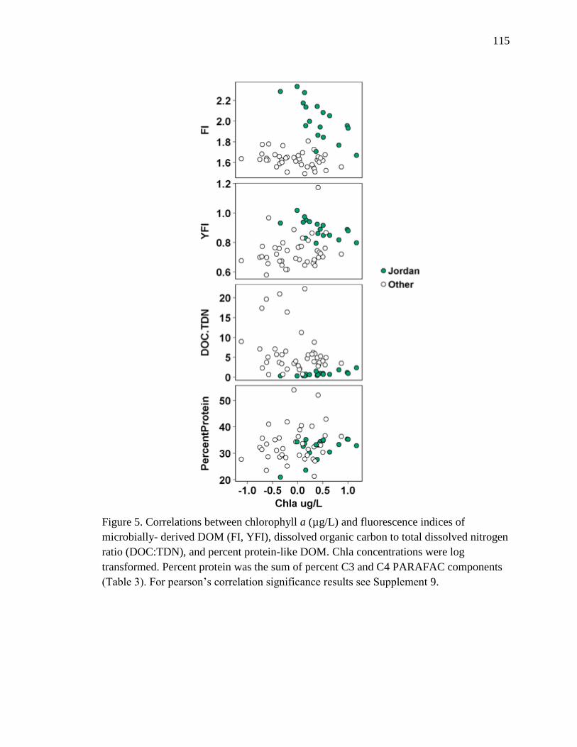
115
Figure 5. Correlations between chlorophyll a (µg/L) and fluorescence indices of
microbially- derived DOM (FI, YFI), dissolved organic carbon to total dissolved nitrogen
ratio (DOC:TDN), and percent protein-like DOM. Chla concentrations were log
transformed. Percent protein was the sum of percent C3 and C4 PARAFAC components
(Table 3). For pearson’s correlation significance results see Supplement 9.

116
Figure 6. Percent feasible contributions of 4 sources to 75 FPOM samples collected in all
watersheds. Contributions were estimated with 3 isotope tracers, δ13C, δ15N, and δ2H. The
autochthonous endmember was the average of algae, biofilm and macrophyte isotope
values (Table 1). Boxes represent 75% high density interval (HDI), the 75% most
credible values, and whiskers represent the 95% HDI.

117
Figure 7. FPOM-δ13C values compared to DIC-δ13C of river water (A), and FPOM -δ2H
values compared to δ2H of river water (B). The solid and dashed lines represent the
average and standard deviation of δ2H and δ13C values of tree leaves; Table 1). If FPOM
was dominated by autochthonous sources, FPOM-δ13C and FPOM-δ2H would vary
linearly with aqueous δ13C and δ2H.

118
Supplement
Supplement 1A. Maps of study sites for Red Butte Creek (n=8, 2nd highest site not
shown) and the Provo River (n=8).

119
Supplement 1B. Study sites on the Logan River (n=8) and Blacksmith Fork (n=1).

120
Supplement 2A. Six land covers were expected to influence OM composition including
wetland, forest, cultivated cropland (crops), pasture, scrub-grassland and development.
These land covers were derived by summing land covers that were ecologically similar
and positively correlated with each other including developed (open+ low+ medium+
high), forest (deciduous + evergreen + mixed), wetland (woody + emergent), scrub-
grassland (Shrub/Scrub + Grassland).

121
Supplement 2B. PCA of land cover by site grouped by watershed.

122
Supplement 3. Contour maps of excitation and emission intensities of the 4 components
resolved by a PRAFAC model with 213 EEMs. Intensities are in Raman units.
Components 1 and 2 (C1, C2) were humic-like and components 3 and 4 (C3,C4) were
protein-like. (B) Split half validation of excitation (dotted lines) and emission (solid
lines) loadings. Validation indicates samples were split into 6 halves and recombined into
3 models and all components in the split models found a match with Tucker correlation
coefficient > .95 (Murphy et al. 2013).

123
Supplement 4. PCA of land cover and sites grouped by watershed and percent
PARAFAC components projected onto the PCA. C1 and C2 were humic-like components
and C3 and C4 were protein-like components (See table 3).

124
Supplement 5.1. Multi-way ANOVAs of water quality metrics, fluorescence indices and
PARAFAC components among watersheds. Tukey HSD significant differences are in the
multiple comparisons table below.

125
Supplement 5.2. Table of Tukey HSD multiple comparisons for ANOVAs of water
quality and DOM fluorescence metrics. DOC and TDN units were mg/L and Chla units
were µg/L.
Watershed Comparison DOC TDN DOC:TDN Chla FI YFI BIX HIX SUVA TC
JR v LR 0 0 0.4 0.03 0 0 0 0.45 0.68 0.11
JR v PR 0 0 0 0.05 0 0 0 0 0 0.03
JR v RB 0 0 0 0 0 0 0 0.01 0.08 0.91
LR v PR 0 0.19 0 1 0.05 0 0 0 0.08 0
LR v RB 0 0.99 0.02 0.11 1 1 0.3 0.28 0.61 0.39
RB v PR 0.01 0.31 0.94 0.06 0.03 0 0 0 0.59 0.01
Watershed Comparison % C1 % C2 % C3 % C4 % Protein
JR v LR 0 0 0 0 0.36
JR v PR 0.01 0 0 1 0.01
JR v RB 0 0 0 0.12 0.99
LR v PR 0 0.12 0.95 0 0
LR v RB 0.14 1 0.07 0.02 0.22 RB v PR 0.19 0.12 0 0.23 0.02

126
Supplement 6. PCA graphs of DOM grouped by watershed and table of covariate
correlations to PC1, PC2, and PC3. Principle components 1(PC1) and 2 (PC2) explained
66% of variation total variation in DOM composition (Figure 2), and PC3 explained
10%. Larger points in 95% confidence ellipses represent the mean of PC1 and PC3
values for sites in a watershed. The table was sorted by correlation to PC1 and values in
bold are signifianct correlations (r > 0.35; Rohlf and Sokal 1995).
Variable PC1
45%
PC2
21%
PC3
10%
r r r
percentC2 -0.90 -0.33 0.13
HIX -0.89 0.22 0.14
DOC:TDN -0.48 0.08 0.22
SUVA -0.47 -0.09 -0.04
percentC1 -0.08 0.96 -0.13
Chla 0.20 0.02 0.76
percentC4 0.31 -0.87 -0.24
FI 0.64 0.47 -0.41
TC 0.72 -0.55 0.09
percentC3 0.76 0.29 0.42
BIX 0.87 0.06 0.20
YFI 0.96 0.05 -0.06

127
Supplement 7. Correlation r squared values for OM-δ13C versus DIC-δ13C, and OM- δ2H,
versus water-δ2H for DOM and FPOM.
DOM OM-δ13C v DIC-δ13C OM- δ2H v water- δ2H
Jordan -0.16 -0.23
Logan -0.54 0.49
Provo -0.4 0.06
Red Butte -0.56 0.13
FPOM Jordan 0.68 -0.19
Logan 0.53 0.03
Provo 0.17 0.39
Red Butte -0.61 -0.11

128
Supplement 8. River water δ18O and δ2H values of 4 watersheds sampled. Most sites fall
along the local meteoric water line (δ2H = 7.45 X δ18O-1.66). Groundwater dominated
sites that receive snow melt at higher elevations had lower δ18O and δ2H values (Logan
River and Provo River) compared to sites at lower elevations (Red Butte) that also
received water with an evaporative signature from Utah lake (Jordan River).

129
Supplement 9. Pearson’s correlation values for chlorophyll a and fluorescence indices by
watershed.

130
CHAPTER IV
DOM DEMAND AND NON-ADDITIVE EFFECTS OF AUTOCHTHONOUS AND
TERRESTRIAL LEACHATES IN BIOASSAYS AND EXPERIMENTAL STREAMS
Abstract: Dissolved organic matter (DOM) is the largest pool of OM in aquatic systems,
and as a primary substrate for microbial respiration in streams, it is important to
understand the drivers of DOM decay. Often, DOM decay measurements are based on
proxies of DOM (e.g. sugar or leaf-litter leachate) or by compartmentalizing DOM into 2
pools of labile and semi-labile DOM. Many DOM decay rates were quantified with
bioassays, which may underestimate DOM decay in streams because they do not include
a benthic zone, and do not account for downstream transport of DOM. In both
experimental streams and dark bottle bioassays we measured decay of 2 types of labile
DOM, algae and light-degraded soil and light-degraded plant leachates, and 2 types of
semi-labile DOM, plant and soil leachates. We also quantified decay rate constants of
labile and semi-labile pools of DOM when mixed to test for non-additive effects, or
priming, of semi-labile DOM by labile DOM. We compared dissolved organic carbon
(DOC) decay from bioassays and experimental streams to previous studies that quantified
DOC loss in bioassays or stream reaches. Bioavailable DOC (BDOC) was greater in
experimental streams (mode 52.6 % ± 20.3),compared to bottle bioassays (mode 22.8% ±
12.3), but there was no significant difference in DOC decay rate constants between

131
bottles and experimental streams. Mixing of labile and semi-labile DOM resulted in both
positive and negative non-additive effects. Consistent non-additive effects were difficult
to quantify due to extremely fast decay of algal (2.06/d ± 0.66), and light-degraded,
terrestrial DOM (1.54/d ± 0.74 ). Decay rates calculated in this study are needed for
models that aim to estimate the proportion and quantity of OM transformed and evaded to
the atmosphere by rivers at the interface of terrestrial and aquatic ecosystems.
Keywords: priming, dissolved organic matter, non-additive effects, light degradation,
first order decay, biexponential decay, biphasic decay, PARAFAC
Introduction
Dissolved organic matter (DOM) is the largest pool of organic matter (OM) in
aquatic ecosystems (Webster and Meyer 1997, Wetzel 2001) and the flux of DOM from
terrestrial ecosystems to inland waters is recognized as an important component of
organic carbon budgets at watershed (Moody et al. 2013) to global scales (Battin et al
2008, Butman et al. 2016). Continental and global estimates show that carbon dioxide
evasion from streams and rivers (hereafter streams) is at least as large as terrestrial net
ecosystem production (Battin et al. 2008, Butman et al. 2016). However, empirical
measures of whole-ecosystem DOM transformations are lacking, and the rate at which
streams process terrestrial DOM inputs remains poorly understood (Battin et al. 2009,
Mineau et al. 2016).

132
Aside from its relation to carbon budgets, it is important to have baseline
estimates of stream DOM transformations for managers who aim to reduce OM loads, as
well as to mitigate for pathogens and contaminants associated with OM in human-altered
watersheds (Edmonds and Grimm 2011, Stanley et al. 2012). DOM can contribute to
biochemical oxygen demand, the formation of disinfection by-products, and adsorb metal
contaminants (Stanley et al. 2012, Kaushal et al. 2014). DOM decay in streams is
controlled by several factors, including hydrologic dilution, sorption to sediments,
microbial metabolism, and photodegradation (Edmonds and Grimm 2011). Managers
may not have control of all these factors, but dilution is a relatively common DOC
reduction strategy (Gücker et al. 2006, Edmonds and Grimm 2011) that may decrease
stream ecosystem functions such as nutrient, pollutant, and pathogen retention, (Bunch
and Bernot 2011, Kaushal et al. 2014). More reach-scale measures of DOM removal,
such as DOC decay, that are valid for use at the watershed scale are needed (Mineau et al.
2016, Seybold and McGlynn 2018), and will inform OM management in streams, as with
similar investigations into nitrate removal in streams (Mulholland et al. 2008).
Bioassays, which include any closed system incubation (e.g. dark bottles,
Erlenmeyer flasks), are commonly used to measure DOM decay as bacterial respiration
and/or organic carbon loss. Bioassay decay rates are problematic because most
incubations do not include a proxy for the benthic zones (benthos) of aquatic systems
(Catalán et al. 2016, Mineau et al. 2016, Bengtsson et al. 2018). These habitats contribute
to at least half of DOM consumption in marine and lake sediments (Bengtsson et al
2018), and at least half of stream DOM demand (Cory and Kaplan 2012, Risse-Buhl et al.
2012, Mineau et al. 2016). In addition, bioassays typically are conducted in the dark, so

133
they do not account for effects of photodegradation. Further, results are difficult to
compare across studies because incubation times vary from days to years, and may or
may not include sediment (van Nugteren et al. 2009), inorganic substrates (e.g. glass
beads; Catalán García et al. 2015, Ward et al. 2016), or circulation to maintain realistic
dissolved oxygen concentrations (Lock and Hynes 1976, Qualls and Haines 1992).
DOM decay rates are difficult to constrain because DOM is a complex, highly
variable mixture of compounds (Seitzinger et al. 2005, Kaplan et al. 2008). The chemical
composition and quality of DOM influences the ability of microbes to consume DOM,
and is therefore an important control of decay rate (Koehler et al. 2012, Mostovaya et al.
2016). The majority of DOM is considered semi-labile (i.e. recalcitrant), derived from
terrestrial sources, such as soil and plant leachates, and is typically rich in humic
constituents (Findlay and Sinsabaugh 2003). The quality of terrestrial DOM can also
change because of exposure to sunlight. Photodegradation can reduce the molecular
weight of DOM constituents but the degree of degradation depends greatly on DOM
chemical composition (Moran and Zepp 2000, Chen and Jaffé 2014). For example, the
greater the proportion of aromatic content, the greater the effect of sunlight on
bioavailability (Moran and Zepp 2000, Tranvik and Bertilsson 2001). The effects of
photodegradation can increase (Moran and Zepp 1997), decrease (Tranvik and Bertilsson
2001), or have no effect (Wiegner and Seitzinger 2001) on DOM lability to microbes.
Autochthonous DOM, OM produced instream by biofilms, filamentous algae, and/or
macrophytes, is considered extremely labile because it consists of low molecular weight,
protein-rich cellular exudates produced during photosynthesis (Guillemette et al. 2013).

134
We do not understand the interactions between labile and semi-labile DOM pools.
When mixed, these two pools are hypothesized to have non-additive effects on microbial
degradation rates (Guenet et al. 2010, Bengtsson et al. 2018). Non-additive effects refer
to a change in decay rates, usually of the semi-labile pool, when 2 pools are mixed
compared to when the 2 pools remain separate (Bengtsson et al. 2018). The concept of
non-additive effects, also referred to as the priming effect, originated in soil science, but
has been proposed by aquatic ecologists as a possible mechanism to explain the rapid
transformation of semi-labile DOM over short distances in stream networks (Hotchkiss et
al. 2014, Mineau et al. 2016). The priming effect in streams is predicted to occur when a
small pool of autochthonous DOM is mixed with the semi-labile pool, which then
accelerates microbial degradation of semi-labile DOM to a faster decay rate than without
the labile DOM (Guenet et al. 2010, Danger et al. 2013).
We had 2 objectives, first to compare decay rate constants of labile and semi-
labile DOM in experimental streams that included a benthic zone, exposure to sunlight,
and constant reaeration versus bottle bioassays that did not include these effects. Second,
we aimed to quantify the non-additive effects of mixing labile and semi-labile DOM in
experimental streams and bioassays. We designed experiments to test 2 hypotheses: 1)
that bioassays in bottles underestimate stream DOM decay because they exclude benthic
microbes, and 2) that semi-labile DOM decay rates are increased by addition of labile
DOM (i.e. priming).
Seven consecutive 3-day experiments were conducted in experimental streams
and in dark-bottles (bioassays). To confirm that semi-labile sources of DOM decayed at a
faster rate than labile DOM we conducted 5 single-source experiments which measured

135
decay of 2 types of semi-labile DOM (soil and plant leachates) and 3 types of labile
DOM (algal derived, light-degraded plant leachate, and light-degraded soil leachate).
Then we converted decay rate constants to uptake lengths and uptake velocities, to
compare DOM uptake in bottles, experimental streams, and previously reported DOM
uptake metrics from previous studies. Following single-source experiments we conducted
2 priming experiments by mixing labile DOM, either algae or light-degraded plant DOM,
with semi-labile, plant DOM (Fig. 1). Decay rates calculated from single-source
experiments were then used to inform 2-compartment models of semi-labile and labile
decay when mixed. We expected DOM decay rates to be faster in streams compared to
bottles, and we expected that DOC decay rates of semi-labile DOM would be faster when
mixed with labile DOM, compared to semi-labile decay rates without labile DOM.
Methods
Experimental streams
Experiments were conducted in 8 experimental streams at the Cary Institute of
Ecosystem Studies Artificial Stream Facility in Millbrook, New York. Streams were
housed in a greenhouse covered with eight mm high-impact double skinned acrylic and
estimated to transmit 84% of photosynthetically active radiation (Acrylic Building
Products, Mississauga, Canada). In all experiments the fiberglass artificial streams (4 x
0.3 x 0.15 m) were filled with 33 L of groundwater that had low levels of DOC (< 1.0
mg/L, Fig. 1). Water in the streams was circulated at 45 rotations/min using stainless
steel paddle wheels propelled by Dayton DC gear motors (Dayton, Niles, Illinois),

136
yielding a mean velocity of 0.6 m/sec. Forty cobbles covered with periphyton were added
to each stream to compare DOC consumption in experimental stream with benthic
biofilms versus bottle-bioassays without biofilms. Cobbles were collected from an open
canopy section of East Branch Wappinger Creek within the Cary Institute of Ecosystem
Studies conservation research area.
Experimental design and leachates
We conducted 5 single-source experiments followed by 2 priming experiments
over the course of 22 days in July 2016. One dark-bottle was incubated in each stream to
compare decay in bottles-bioassays and experimental streams during each 3-day
experiment (Fig. 1). To ensure DOC concentrations declined over time, 4 experimental
streams were covered with cardboard and designated as dark treatments. The remaining 4
streams were not covered and were designated as light treatments. Light streams
experienced natural daily fluctuations in sunlight to observe more realistic decay rates
than in dark treatments, and dark streams were used to eliminate labile DOM production
from photosynthesis and to be more comparable to dark bottles. At the beginning of
single-source experiments, 12 liters of leachate were added at sunset resulting in 26% of
total stream volume as leachate (Fig. 1). Leachates were added at sunset to maximize the
duration of darkness at the beginning of each experiment, and ensure DOC decline in
light treatment streams prior to sunrise when DOC production would begin in light
streams. Single-source experiments were referred to as algae, soil, light-degraded soil
(soil-light), plant, and light-degraded plant (plant-light). For each priming experiment 10
liters of plant leachate were mixed with 4 liters of labile DOM, either as algae (prime-

137
algae experiment) or light-degraded plant leachate (prime-light experiment). After
leachate was added and allowed to mix, 500 mL dark-bottles were filled with
experimental stream water and sampled for constituents at the same time as experimental
streams.
Algal leachate was made by scrubbing the biofilm off cobbles from East Branch
Wappinger Creek within the Cary Institute of Ecosystem Studies conservation research
area and mixing this slurry with groundwater. The leachate was then incubated in 5
gallon buckets for 1-2 hours. Soil leachate was made by mixing 4 liters of soil with 10
liters of groundwater, stirred and allowed to settle for 2-4 hours. Plant leachate was made
from concentrated roasted barley leachate. Barley concentrate was made by adding 60 g
of ground, roasted barley to one liter of groundwater. Plant leachate was then made by
adding 5 mL of concentrate to a liter of groundwater. Light-degraded soil and plant
leachates were made by incubating leachate in 0.5 x 1 x 0.2 m trays in full sun for 3-4
hours. Terrestrial leachates were exposed for what we considered the minimum amount
of time DOM would be exposed to natural sunlight in a temperate stream with a short
travel time (<1 day). All leachates were filter-sterilized using 0.2 µm pore size in-line
cartridge filters (Waterra, Mississauga, Ontario, CA).
DOC was sampled prior to adding leachate and 1, 3, 6, 24, and 70 hours after
leachate additions (Fig. 1). Experimental stream and bottle samples were filtered with 0.7
µm glass fiber filters (Whatman GF/F) into 40 mL amber vials and acidified to a pH of
2.5 for storage until carbon analysis. Acidified DOC samples were run on a Shimadzu
TOC-L analyzer via catalytic oxidation combustion at 720 °C (MDL 0.62 mg/L DOC;
Shimadzu Corp., Kyoto, Japan). Streams and bottles were sampled for

138
spectrofluorometric analysis after 1, 24, and 70 hours. Samples were filtered and stored in
amber vials at 6°C until analysis. Periphyton in the experimental streams were also
collected after 1, 24, and 70 hours to obtain chlorophyll a and ash-free dry mass of
benthic biomass.
DOM fluorescence
Excitation emission matrices (EEMs) were collected on an Aqualog
spectrofluorometer to assess changes in DOM character though each 3-day experiment
and to calculate DOM fluorescence indices that characterized DOM as either microbial or
humic-like. EEMs were collected with excitation wavelengths from 248 to 830 at 6 nm
increments and over emissions 249.4 to 827.7 at 4.7 nm (8 pixel) increments. All samples
were collected in ratio mode (S/R) and run at an integration time resulting in a maximum
emission intensity of 5,000 to 50,000 counts per second. Samples that exceeded 0.3
absorbance at excitation 254 nm were diluted with deionized water. All samples were
corrected for inner filter effects, Rayleigh scatter, and blank subtracted in MATLABTM
(version 6.9; MathWorks, Natick, Massachusetts) as described in Murphy et al (2013).
From EEMs, the fluorescence index (FI), β:α index or freshness index (BIX),
humification index (HIX), and peak T to peak C ratio (TC) were calculated. High versus
low FI values indicate microbial versus terrestrially derived DOM (Cory and McKnight
2005). Higher values of the BIX indicate more recently derived DOM (Parlanti et al.
2000), and more humic-like DOM for higher values of the HIX (Zsolnay et al. 1999). The
TC index represents the ratio of the protein-like peak (T) to humic-like peak (C)
intensities (Baker 2001). SUVA (SUVA), an indicator of DOM aromatic content, was

139
calculated by normalizing the absorbance at 254 nm by the DOC concentration of each
sample (Weishaar et al. 2003).
Parallel factor analysis (PARAFAC) was used to identify fluorescence
components of DOM to assess changes in DOM throughout each experiment (e.g., a
decline in humic-like components due to light exposure). PARAFAC decomposes a
collection of EEMs into groups of organic compounds with similar fluorescent
characteristics (Stedmon and Markager 2005). MATLAB was used to create a
PARAFAC model with 213 EEMS using the drEEM toolbox following Murphy et al.
(2013). The model was then validated with split-half analysis, and resolved components
were compared to previously found fluorophores in the open source library OpenFluor
(Murphy et al. 2014). Percentage of each PARAFAC component was correlated with
fluorescence indices using Pearson correlations in R with the psych v1.7.8 package
(Revelle 2017).
Five linear models were run to identify treatments that best described variation in
fluorescence indices and PARAFAC components. Linear models tested the fixed effects
of 1) treatment, 2) treatment plus bottles versus streams, 3) treatment light streams versus
dark streams, and 4) the interaction of treatment and light versus dark streams. Samples
collected after 70 hours were used to assess differences in fluorescence indices and
PARAFAC components since that is when differences were greatest. Bayes factors were
calculated to identify the linear model that best described variation in dependent
variables. The Bayes factor (B01) can be generalized as the probability ratio between two
models (𝑀0, 𝑀1) (Eqn. 1).

140
𝐵01 =
Pr(Data|𝑀0)
Pr(Data|𝑀1)
(1)
The R package BayesFactor was used with uninformative priors (Morey et al. 2018).
Bayes factors were calculated for models normalized by the effect of treatment alone.
Significant differences in treatments were then tested using multiple comparisons of
means and Tukey HSD.
DOC decay models
To estimate decay rates constants for single-source experiments we used an
inverse modeling approach with Bayesian parameter estimation. Decay rates constants
were calculated for all experiments after 6, 24, and 70 hours. Single-source decay rates
were estimated using a first order exponential decay model (Eqn. 2):
𝐶𝑡 = 𝐶0𝑒−𝑘𝑡𝑜𝑡𝑡 (2)
where 𝐶0 and 𝐶𝑡 represent DOC concentrations at the start and end of the period
over which −𝑘𝑡𝑜𝑡 was calculated over time (𝑡). The difference in mean decay rates for
labile and semi-labile DOM estimated from single-sources models were then used to test
the hypothesis that labile sources of DOM (algae, soil-light, plant-light) decayed faster
than semi-labile sources (soil, plant). The difference was calculated by subtracting the
95% high density interval (HDI) of semi-labile DOM from the 95% HDI of labile DOM.
If the median difference was greater than zero the decay rates were considered
significantly different (Hotchkiss et al. 2014). Parameter values within the 95% HDI are
more likely than outside the HDI, and all values within the HDI represent 95% of all
possible values (Kruschke 2015).

141
Two different models were used to estimate DOC decay rates in priming
experiments. First, a two-compartment, biexponential decay model assumed the labile
(𝑘𝑓𝑎𝑠𝑡), and semi-labile (𝑘𝑠𝑙𝑜𝑤), pools of DOC decayed simultaneously starting at time
zero 𝑡0 (Eqn. 3):
𝐶𝑡 = 𝑝1𝐶1(𝑡0)𝑒−𝑘𝑓𝑎𝑠𝑡𝑡 + 𝑝2𝐶2(𝑡0)𝑒−𝑘𝑠𝑙𝑜𝑤𝑡 (3)
where 𝐶𝑡 is the total concentration of both labile (𝐶1), and semi-labile (𝐶2), pools at the
start of the experiment, and 𝑝1and 𝑝2 are the proportional volumes of each leachate
(Hotchkiss et al 2014; Supplement 1).
Second, a 2-compartment, biphasic decay model assumed there was a fast period
of decay, followed by a slow period of decay (Eichmiller et al. 2016, Brouwer et al.
2017). For the biphasic model, 𝑘𝑓𝑎𝑠𝑡 was estimated using first order exponential decay up
to a breakpoint at time 𝑡∗ (Eqn. 4), and 𝑘𝑠𝑙𝑜𝑤was estimated for the period of decay after
the breakpoint using the value estimated for 𝑘𝑓𝑎𝑠𝑡 prior to the breakpoint (Eqn. 5;
Supplement 1).
𝐶𝑡∗ = 𝐶0𝑒−𝑘𝑓𝑎𝑠𝑡𝑡 𝑡 < 𝑡∗ (4)
𝐶𝑡 = 𝐶0𝑒−𝑘𝑓𝑎𝑠𝑡𝑡∗𝑒−𝑘𝑠𝑙𝑜𝑤(𝑡−𝑡∗) 𝑡 > 𝑡∗ (5)
There were not enough time points to identify the breakpoint between fast and slow
periods of decay using traditional methods of breakpoint analysis (e.g., segmented or
changepoint analysis). Therefore, breakpoints were estimated visually from raw DOC
concentrations plotted over 70 hours.
The decay rates of each compartment were estimated using Bayes Rule where the
posterior probability distribution of 𝑘𝑓𝑎𝑠𝑡 and 𝑘𝑠𝑙𝑜𝑤, given the DOC data, is proportional
to the product of the likelihood of the decay model, and the prior probability distributions

142
of the decay parameters (Hotchkiss et al 2014). The posterior probability distributions of
𝑘𝑓𝑎𝑠𝑡 and 𝑘𝑠𝑙𝑜𝑤 were simulated with the rjags package using Markov Chain Monte Carlo
(MCMC) sampling from an informed prior distribution (Plummer 2018). Each model was
run for 150,000 iterations, using three different starting values for each chain, and the
first 10,000 samples were not included in parameter estimation. Model fit was assessed
through linear regression of measured versus predicted values of DOC concentrations at
the last modeled time point.
To determine if positive non-additive effects were significant (priming effect), we
subtracted the posterior probability distribution for single-source plant decay (𝑘𝑡𝑜𝑡) from
the posterior distribution of the slow-decay compartment (𝑘𝑠𝑙𝑜𝑤). A positive non-additive
was considered significant if the median difference in the 95% HDI of the two
distributions (𝑘𝑠𝑙𝑜𝑤 − 𝑘𝑡𝑜𝑡) was greater than zero (Hotchkiss et al. 2014).
Bioassay versus experimental stream DOC decay
To test the hypothesis that bioassays underestimate DOC decay, differences in
single-source DOC decay constants and BDOC were compared using the BEST test
(Bayesian estimation superseded t-Test) in R (Kruschke 2013). If the difference in
posterior probability densities estimated for the mean of each group includes zero, the
BEST test is considered not significant. BDOC was calculated as the percent loss in DOC
concentration from 3 to 70 hours in streams (Fellman et al. 2008). BDOC in bottles and
streams was calculated from 6 to 70 because, for the first 6 hours of 4 experiments, DOC
concentrations increased due to DOM production, (as seen previously Hosen et al. 2014)
after which concentrations declined for the duration of the experiment. To further

143
compare bioassays and stream DOM decay, we compared DOM decay rate constants
from studies that used bottles (Hotchkiss et al. 2014) to decay rate constants calculated
from stream reach additions (Webster and Meyer 1997, Griffiths et al. 2012, Epstein et al.
2016, Hall et al. 2016; Supplement 2).
Benthic biomass
Benthic biomass was measured to assure that any differences in DOM decay were
due to differences in DOM source rather than biomass effects. To collect periphyton
biomass one cobble was taken from each experimental stream after 1, 24, and 70 hours,
scrubbed with a toothbrush and washed with an aliquot of groundwater. Periphyton slurry
from each cobble was subsampled and filtered through GF/F filters and analyzed for
chlorophyll a and ash free dry mass (AFDM) analysis following Steinman et al. (2007).
A picture of each cobble was taken to calculate surface area using ImageJ (Schneider et
al. 2012). Chlorophyll a and AFDM then were normalized by area of each cobble
sampled. We detected no significant differences across experiments in benthic biomass
measured as AFDM which confirmed that biomass did not factor into differences among
experiments (Supplement 3). Chlorophyll a concentrations were lower in priming
experiments than single-source experiments, but did not differ among other experiments
(Supplement 3). As priming experiments occurred at the end of the 22 day period during
which the experiments were conducted, we interpret this to indicate aging of the biofilm.
Benthic biomass data are not discussed further in this paper (see Supplement 3).

144
Results
Were decay rates of algal labile DOM faster than semi-labile DOM?
To confirm the hypothesis that labile DOM decay rates (algae and light-degraded)
were faster than semi-labile DOM decay rates (soil and plant) we tested the difference
between estimated values of labile and semi-labile decay rates (Table 1, Supplement 4).
The difference in mean decay rates of light versus dark treatments of experimental
streams were not significantly different after 6 hours (95 %, HDI -2.61, 3.96), 24 hours
(HDI -0.99, 0.45) or 70 hours (HDI -0.38, 0.23; Supplement 5). Therefore, we assessed
decay rates among treatments for all 8 streams combined.
Algal DOM decay rates were always faster than soil and plant DOM decay rates
in both bottles and streams, except after 70 hours, algal decay was not faster in streams
(Table 1, Supplement 4). Soil and soil-light DOM decay rates were highly variable in
streams, and there was little to no decay of both treatments in bottles. Light-degraded
plant DOM decay rates were faster than soil and plant decay rates over the first 6 hours of
the experiment but were not significantly faster after 24 and 70 hours in both bottles and
streams. Overall labile DOM decay rates of algal and plant-light DOM were hard to
estimate (i.e. high variation) in the first 6 to 24 hours of each experiment, and their decay
rates declined significantly after 70 hours.
Did sunlight alter DOM composition?
DOM composition Fluorescence indices were calculated to characterize DOM from
different leachates and to identify changes in DOM composition during each experiment.
In all experiments, FI values were higher in light streams (mean 1.65, sd 0.09) than dark

145
streams (mean 1.61, sd 0.09) indicating more microbial-derived DOM in light streams
(Fig. 2). SUVA and HIX values were significantly lower in the soil-light experiment than
the soil experiment indicating a decrease in aromatic content of soil-derived DOM after
exposure to sunlight (Fig2, Supplement 6). Likewise, indices of recently derived DOM
(BIX) and protein-like DOM (TC) were higher in the soil-light than soil experiment
(Supplement 6). Plant DOM had lower aromatic content (SUVA mean 0.63, sd 0.19) than
algal and soil derived DOM (SUVA mean 3.02 sd 2.9; mean 2.6, sd 0.29; Fig. 2).
A 5 component PARFAC model (hereafter C1 to C5) was resolved and validated
with split-half analysis to identify major fluorophores (Supplement 7). Components 1
through 5 were at least 95% identical to fluorophores identified within the OpenFluor
library (Murphy et al. 2014). C1, C2, and C3 were described as humic-like in previous
studies and this study (Table 2). Earlier studies described C4 as recently transformed or
microbial-derived (Murphy et al. 2013). In this study, percent C4 was greatest for plant
derived DOM (Fig. 3) which had less aromatic content than soil DOM (Fig. 2), and was
more recently derived than soil DOM as indicated by higher BIX values than soil derived
DOM (Supplement 6). C5 was protein derived, tryptophan-like DOM in both this, and
previous studies (Coble et al 1996, Yamashita and Tanoue 2003).
Percent C2 was lower in light streams at the end of all experiments, except the
algae experiment, indicating it was susceptible to light degradation in terrestrially derived
DOM (Fig. 3). The greatest concentrations of C3 were in the soil and soil-light
experiments (range 23-29%) were associated with older humic DOM because C3 was
positively correlated with the HIX and SUVA (r = 0.64, r = 0.75; Supplement 8). C3
appeared to be “produced” from light exposure as it increased in proportion to other

146
components in the light streams of all plant experiments (Fig. 3). But, C3 also increased
slightly in dark streams with plant DOM, therefore microbial activity that consumed C2
may have created C3 in the process. C4 had highest concentrations in plant experiments
(range 24 to 31%) and was negatively correlated with the HIX and SUVA (r =-0.72, r = -
0.81; Supplement 8). C5 the protein-like component, declined in all experiments except
for the soil experiment which had the lowest percent protein out of all experiments (range
10-16%).
Do bioassays underestimate microbial DOM demand when compared to
experimental or real streams?
To assess whether DOM consumption measured in bioassays was comparable to
that measured in experimental streams, we compared DOC decay rate constants, and
BDOC between bioassays versus experimental streams, and bioassay versus experimental
streams and real streams. Decay rate constants were excluded from comparisons if the
coefficient of variation (CV) among 8 streams and bottles within a treatment were greater
than 100% to ensure only consistently estimated decay rates were used in comparisons.
Excluded decay rate constants included 2 experimental stream decay rates calculated
after 24 hours (CV SoilLight 128% and Soil 287%) and 4 bottle decay rates (Plant -24
hrs 183%, Soil-70 hrs 377%, SoilLight-70 hrs 612%, Soil-24 hrs 866%). Again, there
was no difference in mean decay of light versus dark experimental streams, so results
from light and dark experimental streams were pooled (Supplement 4).
Decay rate constants Decay rates constants from single-source experiments of
experimental streams (n= 13, mode 0.23/d, sd 0.89) were not different from decay rate

147
constants of bioassays (n = 11, mode 0.199 /d, sd 0.527; 95 % HDI -0.426, 0.901; Fig. 4).
Decay rate constants of bioassays in previous studies tended to be lower (n = 33,
0.041/d, sd 0.028), than for real streams (n = 25, mode 0.003/d, sd 0.004), but the
probability density of difference in means included zero ( 95 % HDI -0.004, 0.057), and
therefore was not significant.
Bioavailable DOC BDOC was calculated to compare the proportion of DOC lost
during each single-source experiment between bottles and experimental streams. Soil
leachate BDOC in streams was significantly lower (<0 %) than all other experimental
stream experiments, and there were no other significant differences in BDOC among
treatment experiments in streams (F = 0.94, p = 0.46). Overall, percent BDOC was
greater in streams (mode 52.6 %, sd 20.3) than bottles (mode 22.8%, sd 12.3; 95 % HDI
22.6, 36.7; Fig. 5).
Do positive non-additive effects result from mixing DOM pools?
We used plant-leachate as the semi-labile source of DOM in priming experiments
because single-source soil leachate experiments reached maximum concentrations of ca.
4 mg/L DOC so it was difficult to detect significant declines in DOC concentrations and
estimate decay rates for soil leachate. Variation in single-source estimates of plant
leachate decay in bottles were extremely high (CV mean 111%) compared to
experimental streams (CV mean 20%), so meaningful effect sizes for non-additive
effects in bottles could not be calculated, and are not discussed further.
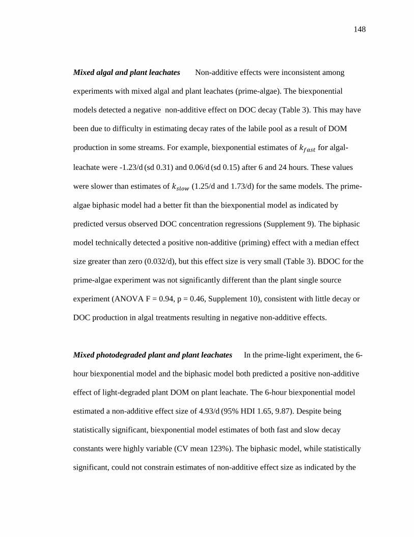
148
Mixed algal and plant leachates Non-additive effects were inconsistent among
experiments with mixed algal and plant leachates (prime-algae). The biexponential
models detected a negative non-additive effect on DOC decay (Table 3). This may have
been due to difficulty in estimating decay rates of the labile pool as a result of DOM
production in some streams. For example, biexponential estimates of 𝑘𝑓𝑎𝑠𝑡 for algal-
leachate were -1.23/d (sd 0.31) and 0.06/d (sd 0.15) after 6 and 24 hours. These values
were slower than estimates of 𝑘𝑠𝑙𝑜𝑤 (1.25/d and 1.73/d) for the same models. The prime-
algae biphasic model had a better fit than the biexponential model as indicated by
predicted versus observed DOC concentration regressions (Supplement 9). The biphasic
model technically detected a positive non-additive (priming) effect with a median effect
size greater than zero (0.032/d), but this effect size is very small (Table 3). BDOC for the
prime-algae experiment was not significantly different than the plant single source
experiment (ANOVA F = 0.94, p = 0.46, Supplement 10), consistent with little decay or
DOC production in algal treatments resulting in negative non-additive effects.
Mixed photodegraded plant and plant leachates In the prime-light experiment, the 6-
hour biexponential model and the biphasic model both predicted a positive non-additive
effect of light-degraded plant DOM on plant leachate. The 6-hour biexponential model
estimated a non-additive effect size of 4.93/d (95% HDI 1.65, 9.87). Despite being
statistically significant, biexponential model estimates of both fast and slow decay
constants were highly variable (CV mean 123%). The biphasic model, while statistically
significant, could not constrain estimates of non-additive effect size as indicated by the

149
broad posterior probability density around the estimated median of 0.88/d (95% HDI -
0.76, 2.99). While BDOC tended to be higher in streams in the prime-light versus plant
experiment, there was no significant difference between experiments (Supplement 10).
Discussion
Bioassays may underestimate DOC demand in streams
Average BDOC in experimental streams was 2 times greater than in bottles,
which suggests bioassays underestimated DOC decay in experimental streams.
Experimental stream BDOC was similar to the estimated percent DOC consumed at the
watershed scale which ranged from 27 to 45% for 7 north-east watersheds (Mineau et al.
2016). Bioassay decay rate constants also tended to be slower than decay rates calculated
from mass balance models at the watershed scale, but the ideal comparison to test our
hypothesis would compare bioassay decay rates constants calculated from mass balance
models to decay rate constants calculated for ambient DOM in bioassays from the same
watershed. While we cannot conclude if bioassays underestimated DOC demand in real
streams, evidence suggests given then same OM substrate, bioassays would likely
underestimate DOM demand compared to a lotic system with a benthic component.
In addition, first order decay rates estimated from bioassays and experimental
streams include products of microbial production less than 0.7 µm, or whatever filter pore
size is used to collect DOM. As a result, decay rate constants estimated were based on net
changes in DOC concentration, not gross DOC consumption, another factor to suggest
such experiments underestimate DOM demand. Without an isotope tracer, DOC demand

150
estimated from bulk DOM additions is likely not comparable to DOM demand in lotic
ecosystems. Thus, the role of bioassays and experimental streams as a tool to predict
carbon cycling at the watershed scale needs further study (Mineau et al. 2016) to help
further constrain estimates of DOM transformation in rivers.
We recommend future studies of stream DOM supplement bioassay decay rates
with additional measures of DOC mineralization such as reach-scale measurements
and/or mass balance models. Bioassays not only exclude DOC consumption by benthic
biofilms, they also exclude the effect of abiotic factors that increase DOC decay such as
photodegradation, adsorption, and sedimentation (Cory and Kaplan 2012, Catalan et al.
2016). As noted by Catalan et al. (2016), field studies better integrate all processes of
DOC loss and production which may have minimal consequences for bioassays of
aquatic systems with long water residence times (e.g. > 1 year), but could significantly
influence bioassay decay rates in water bodies with short residence times such as streams.
Our study would have benefitted from an experimental stream control without benthic
periphyton to help elucidate physical versus biological drivers of DOC decay.
Supplementing bioassays with field studies, or lotic mesocosms, such as experimental
streams or plug-flow reactors, would help account for all physical and biological factors
that influence DOC decay in streams.
Extremely fast labile DOM decay
Our estimates of decay for labile sources of DOM in experimental streams, (i.e.
algae and light-degraded plant) were an order of magnitude greater than estimates of
labile pools calculated from previous bioassays and field-based models (Griffiths et al.

151
2012, Hotchkiss et al. 2014, Epstein et al. 2016, Hall et al. 2016). For both bottles and
experimental streams, decay rate constants were faster when calculated within the first 6
or 24 hours of the experiment compared to 70 hours. Few studies have estimated DOM
decay within the first 12 to 24 hours of incubation (but see Lyon and Zeigler 2009, Cory
et al. 2007). Incubation durations range over days (Bernhardt and Likens 2002, Hotchkiss
et al. 2014), weeks (Guillemette and del Giorgio 2011, Catalan et al. 2015), months
(Danger et al. 2013) and years (Vahatalo and Wetzel 2008, Evans et al. 2017). The only
study to report a decay rate constant faster than this study was for the labile portion of
stream DOM incubated in bioreactors with an empty bed contact time < 15 min. resulting
in a decay rate constant of 1.59/day and uptake velocity of 1.23 mm/min (Kaplan et al.
2008). While most DOM decay studies assume a constant first order decay rate
(Guillemette et al. 2013), if differences in decay rate constants depend on the time over
which decay is calculated, as in this study, first order decay may not be an appropriate
model of DOC decay. Recent DOM decay studies have investigated the reactivity
continuum model that assumes overall decay is the result of an infinite number of
reactive pools with decay constants that decrease over time and indeed found that decay
rates vary over time (Koehler et al. 2012, Guillemette et al. 2013).
Regardless of the model used to describe decay, labile DOM pools in freshwater
are known to decay within hours to one day (Guillemette and del Giorgio 2011, Cory and
Kaplan 2012, Hotchkiss et al. 2014, Mostovaya et al 2016, Ward et al. 2016), or even
within minutes (Pollard et al 2013). Future studies that aim to quantify consumption of
autochthonous DOM, or other labile DOM, should increase sampling frequency and
replication within the first 24 hours of experiments. Furthermore, it may be impossible to

152
measure the most bioavailable DOM in streams since it is consumed so quickly
(Hotchkiss et al. 2014). Bulk DOM samples that are typically collected from streams
likely constitute only the semi-labile DOM that remains “leftover” after labile DOM has
been consumed (Hotchkiss et al. 2014, Findlay and Parr 2017).
Light reduced aromatic content in soil leachate
Exposure to natural sunlight decreased aromatic content in DOM and increased
BDOC of light-degraded soil compared to the single-source soil experiment. Our indices
of DOM degradation by natural sunlight may differ from previous studies because
sunlight exposure time was much shorter than previous experiments. One other study,
conducted in streams, found significant changes in tyrosine-like DOM within 4 to 7 hours
of sunlight exposure (Cory et al. 2007), but most studies investigated the effect of light
over 24 to 48 hours (Skully et al. 2004, Bittar et al. 2015) or up to 5 weeks (Guillemette
and del Giorgio 2011, Catalán et al. 2015). Our study highlights the effect sunlight had on
DOM quality after just 3 to 4 hours of exposure, a duration that represented the minimum
duration of sunlight exposure for a stream in the warm months, of a temperate ecosystem.
Non-additive effects were difficult to quantify
It was hard to quantify the non-additive effect of mixing labile and semi-labile
DOM because it was difficult to measure net DOM decay. All but 2 experiments included
DOM production after leachate was added resulting in highly variable decay rates that
may have underestimated the total amount of DOM assimilated or mineralized. We did
not account for DOM production (as in Hosen et al. 2014), which may have reduced

153
variation in estimates of single-source decay, and therefore could have better informed
biexponential models. The biphasic model better predicted final DOC concentrations for
both non-additive effects experiments because, as opposed to the biexponential model,
the labile and semi-labile pool were distinctly separated by the modeler. A stable isotope
tracer of terrestrially derived DOM would have helped differentiate fast and slow pools
and therefore models could have better estimated fast versus slow decay rates.
While non-additive effects on DOM decay have been studied in soil ecosystems
since the mid 1900s (Bingeman et al. 1953), interactive effects of labile and semi-labile
DOM in aquatic ecosystems have only been studied over the last decade (Guenet et al.
2010, Bengtsson et al. 2018). A recent review identified 17 studies since 2010 that
explicitly tested for non-additive effects in aquatic ecosystems, and found 7 studies
measured a positive non-additive effect, 6 did not, and 4 had mixed results (Bengtsson et
al. 2018). It is worth noting that all studies were conducted as lab incubations, and 65%
of studies used naturally occurring labile OM such as algal leachates, while the other
studies used glucose or other simple compounds (Bengtsson et al. 2018). Laboratory
conditions and the use of non-natural DOM reiterate the difficulty of separating labile
and semi-labile pools due the high variability and complexity of DOM. In addition,
studies of non-additive effects that include a benthic component are vastly
underrepresented in the literature (Bengtsson et al. 2018). We conclude if positive non-
additive effects do occur in aquatic systems, it is extremely hard to detect because
variation in DOM lability is so great that it remains difficult to model separate decay
rates of 2 different DOM pools.

154
Conclusions
It is important to quantify DOM decay and compare decay rates among
ecosystems to better estimate carbon fluxes to the atmosphere from freshwater
ecosystems. The relative lability and processing rate of autochthonous and terrestrial OM
sources remains elusive. Our results emphasize the need to better quantify both fast and
slow decaying OM pools in streams. Direct measurements of known sources of DOM in
an experimental setting can help define the lability of DOM along a continuum of
minutes to years, rather than from correlations of chemical and biological parameters of
DOM to infer lability (Cory and Kaplan 2012, Koehler et al. 2012). More empirical
measurements of OM decay and carbon spiraling metrics for pools with varying lability
will help predict the biological implications of DOM processing in streams.
Excessive OM in streams is a problem worldwide that contributes to cultural
eutrophication, the transport of contaminants to downstream waters, and can increase the
cost of wastewater treatment (Chow et al. 2005, Volkmar and Dahlgren 2006, Solomon et
al. 2015). In addition to informing models of organic carbon flux from streams, better
estimates of DOM decay in streams from varying sources can inform management
decisions aimed at reducing DOM loads at the watershed-scale. If autotrophic production
in human altered watersheds is increased, it is likely the proportion of autochthonously
derived, labile DOM compared to the proportion of semi-labile DOM is also increased. A
greater proportion of labile DOM could saturate microbial demand, and therefore more
semi-labile DOM would remain untransformed and transported downstream to receiving
waters. If managers are to mitigate increased OM loads in rivers, the rate at which labile
and semi-labile DOM is transformed, and the interactive effects of these pools on bulk

155
DOM transformation are useful information for managers. The study of novel sources of
DOM in anthropogenically altered landscapes is just beginning, and baseline measures of
autochthonous and terrestrial rates of DOM decay will help put the ecological
implications of less studied sources of DOM in perspective.
Acknowledgements
We would like to thank the scientists and staff of the Cary Institute of Ecosystem
Studies for their help at the Artificial Stream Facility, as well as Lindsay Capito, Autumn
Slade, and Dave Epstein for their help in the laboratory. The manuscript was improved by
thoughtful comments from Zachary Aanderud, Bethany Neilson, John Stark and Matt
Milller. We thank our funders at Utah State University, including the School of Graduate
Studies, Department of Biology, and Ecology Center. This research was also supported
by the National Science Foundation (awards IIA 12-08732 and DEB 17-54216).
156
Literature Cited
Alexander, R. B., R. A. Smith, and G. E. Schwarz. 2000. Effect of stream channel size on
the delivery of nitrogen to the Gulf of Mexico. Nature 403:758-761.
Attermeyer, K., J. Tittel, M. Allgaier, K. Frindte, C. Wurzbacher, S. Hilt, N. Kamjunke,
and H.-P. Grossart. 2015. Effects of light and autochthonous carbon additions on
microbial turnover of allochthonous organic carbon and community composition.
Microbial Ecology 69:361-371.
Baker, A. 2001. Fluorescence excitation− emission matrix characterization of some
sewage-impacted rivers. Environmental Science and Technology 35:948-953.
Baker, M. A., and J. R. Webster. 2017. Conservative and Reactive Solute Dynamics.
Pages 129-145 in F. R. Hauer and G. A. Lamberti (editors). Methods in Stream Ecology.
Elsevier, Amsterdam.
Battin, T. J., L. A. Kaplan, S. Findlay, C. S. Hopkinson, E. Marti, A. I. Packman, J. D.
Newbold, and F. Sabater. 2008. Biophysical controls on organic carbon fluxes in fluvial
networks. Nature Geoscience 1:95-100.
Battin, T. J., L. A. Kaplan, S. Findlay, C. S. Hopkinson, E. Marti, A. I. Packman, J. D.
Newbold, and F. Sabater. 2009. Biophysical controls on organic carbon fluxes in fluvial
networks. Nature Geoscience 1:95-100.
Bengtsson, M. M., K. Attermeyer, and N. Catalán. 2018. Interactive effects on organic
matter processing from soils to the ocean: are priming effects relevant in aquatic
ecosystems? Hydrobiologia 822:1-17.
Bernhardt, E. S., and G. E. Likens. 2002. Dissolved organic carbon enrichment alters
nitrogen dynamics in a forest stream. Ecology 83:1689-1700.
Bertilsson, S., and L. J. Stefan. 1998. Photochemically produced carboxylic acids as
substrates for freshwater bacterioplankton. Limnology and Oceanography 43:885-895.
Bianchi, T. S. 2011. The role of terrestrially derived organic carbon in the coastal ocean:
A changing paradigm and the priming effect. Proceedings of the National Academy of
Sciences 108:19473-19481.
Bianchi, T. S., D. C. Thornton, S. A. Yvon‐Lewis, G. M. King, T. I. Eglinton, M. R.
Shields, N. D. Ward, and J. Curtis. 2015. Positive priming of terrestrially derived
dissolved organic matter in a freshwater microcosm system. Geophysical Research
Letters 42:5460-5467.

157
Bingeman, C. W., J. Varner, and W. Martin. 1953. The Effect of the Addition of Organic
Materials on the Decomposition of an Organic Soil. Soil Science Society of America
Journal 17:34-38.
Bittar, T. B., A. A. Vieira, A. Stubbins, and K. Mopper. 2015. Competition between
photochemical and biological degradation of dissolved organic matter from the
cyanobacteria Microcystis aeruginosa. Limnology and Oceanography 60:1172-1194.
Blagodatskaya, E., T. Yuyukina, S. Blagodatsky, and Y. Kuzyakov. 2011. Three-source-
partitioning of microbial biomass and of CO2 efflux from soil to evaluate mechanisms of
priming effects. Soil Biology and Biochemistry 43:778-786.
Brouwer, A. F., M. C. Eisenberg, J. V. Remais, P. A. Collender, R. Meza, and J. N.
Eisenberg. 2017. Modeling biphasic environmental decay of pathogens and implications
for risk analysis. Environmental Science and Technology 51:2186-2196.
Bunch, A. R., and M. J. Bernot. 2011. Distribution of nonprescription pharmaceuticals in
central Indiana streams and effects on sediment microbial activity. Ecotoxicology 20:97-
109.
Burd, A. B., S. Frey, A. Cabre, T. Ito, N. M. Levine, C. Lønborg, M. Long, M. Mauritz,
R. Q. Thomas, and B. M. Stephens. 2016. Terrestrial and marine perspectives on
modeling organic matter degradation pathways. Global Change Biology 22:121-136.
Butman, D., S. Stackpoole, E. Stets, C. P. McDonald, D. W. Clow, and R. G. Striegl.
2016. Aquatic carbon cycling in the conterminous United States and implications for
terrestrial carbon accounting. Proceedings of the National Academy of Sciences 113:58-
63.
Catalán García, N., A. M. Kellerman, H. Peter, F. Carmona Pontaque, and L. J. Tranvik.
2015. Absence of a priming effect on dissolved organic carbon degradation in lake water.
Limnology and Oceanography 60:159-168.
Catalán, N., R. Marcé, D. N. Kothawala, and L. J. Tranvik. 2016. Organic carbon
decomposition rates controlled by water retention time across inland waters. Nature
Geoscience 9:501-504.
Chapra, S., and G. Pelletier. 2008. QUAL2Kw theory and documentation (version 5.1) A
modeling framework for simulating river and stream water quality. Environmental
Assessment Program, Washington State University, Olympia, WA.
Chen, M., and R. Jaffé. 2014. Photo-and bio-reactivity patterns of dissolved organic
matter from biomass and soil leachates and surface waters in a subtropical wetland.
Water Research 61:181-190.

158
Chen, M., and R. Jaffé. 2016. Quantitative assessment of photo-and bio-reactivity of
chromophoric and fluorescent dissolved organic matter from biomass and soil leachates
and from surface waters in a subtropical wetland. Biogeochemistry 129:273-289.
Chow, A. T., S. Gao, and R. A. Dahlgren. 2005. Physical and chemical fractionation of
dissolved organic matter and trihalomethane precursors: A review. Journal of Water
Supply: Research and Technology-AQUA 54:475-507.
Coble, P. G. 1996. Characterization of marine and terrestrial DOM in seawater using
excitation-emission matrix spectroscopy. Marine Chemistry 51:325-346.
Cole, J. J., and N. F. Caraco. 2001. Carbon in catchments: connecting terrestrial carbon
losses with aquatic metabolism. Marine and Freshwater Research 52:101-110.
Cory, R. M., and D. M. McKnight. 2005. Fluorescence spectroscopy reveals ubiquitous
presence of oxidized and reduced quinones in dissolved organic matter. Environmental
Science and Technology 39:8142-8149.
Cory, R. M., and L. A. Kaplan. 2012. Biological lability of streamwater fluorescent
dissolved organic matter. Limnology and Oceanography 57:1347-1360.
Cory, R. M., B. C. Crump, J. A. Dobkowski, and G. W. Kling. 2013. Surface exposure to
sunlight stimulates CO2 release from permafrost soil carbon in the Arctic. Proceedings of
the National Academy of Sciences 110:3429-3434.
Cory, R. M., D. M. McKnight, Y. P. Chin, P. Miller, and C. L. Jaros. 2007. Chemical
characteristics of fulvic acids from Arctic surface waters: Microbial contributions and
photochemical transformations. Journal of Geophysical Research: Biogeosciences 112:1-
12.
Danger, M., J. Cornut, E. Chauvet, P. Chavez, A. Elger, and A. Lecerf. 2013. Benthic
algae stimulate leaf litter decomposition in detritus‐based headwater streams: a case of
aquatic priming effect? Ecology 94:1604-1613.
Davis, J., and R. Benner. 2007. Quantitative estimates of labile and semi‐labile dissolved
organic carbon in the western Arctic Ocean: A molecular approach. Limnology and
Oceanography 52:2434-2444.
Edmonds, J. W., and N. B. Grimm. 2011. Abiotic and biotic controls of organic matter
cycling in a managed stream. Journal of Geophysical Research: Biogeosciences 116:
G02015.
Eichmiller, J. J., S. a. E. Best, and P. W. Sorensen. 2016. Effects of temperature and
trophic state on degradation of environmental DNA in lake water. Environmental Science
and Technology 50:1859-1867.

159
Epstein, D. M., J. E. Kelso, and M. A. Baker. 2016. Beyond the urban stream syndrome:
organic matter budget for diagnostics and restoration of an impaired urban river. Urban
Ecosystems 19:1041-1061.
Evans, C. D., M. N. Futter, F. Moldan, S. Valinia, Z. Frogbrook, and D. N. Kothawala.
2017. Variability in organic carbon reactivity across lake residence time and trophic
gradients. Nature Geoscience 10:832-835.
Fellman et al. 2008. Flourescent characteristics and biodegradability of dissolved organic
matter in forest and wetland soild from coastal temperate watersheds in southeast Alaska.
Biogeochemistry 88:166-184.
Fellman, J. B., E. Hood, R. T. Edwards, and J. B. Jones. 2009. Uptake of allochthonous
dissolved organic matter from soil and salmon in coastal temperate rainforest streams.
Ecosystems 12: 747-759.
Findlay, S., and R. L. Sinsabaugh. 2003. Aquatic Ecosystems: Interactivity of Dissolved
Organic Matter. Academic Press, San Diego, CA.
Findlay, S. E. G., and T. B. Parr. 2017. Dissolved Organic Matter. Pages 21-35 in F. R.
Hauer and G. A. Lamberti (editors). Methods in Stream Ecology. Elsevier, Amsterdam.
Fontaine, S., S. Barot, P. Barré, N. Bdioui, B. Mary, and C. Rumpel. 2007. Stability of
organic carbon in deep soil layers controlled by fresh carbon supply. Nature 450:277-280.
Griffiths, N. A., J. L. Tank, T. V. Royer, T. J. Warrner, T. C. Frauendorf, E. J. Rosi-
Marshall, and M. R. Whiles. 2012. Temporal variation in organic carbon spiraling in
Midwestern agricultural streams. Biogeochemistry 108:149-169.
Guenet, B., M. Danger, L. Abbadie, and G. Lacroix. 2010. Priming effect: bridging the
gap between terrestrial and aquatic ecology. Ecology 91:2850-2861.
Guenet, B., M. Danger, L. Harrault, B. Allard, M. Jauset-Alcala, G. Bardoux, D. Benest,
L. Abbadie, and G. Lacroix. 2013. Fast mineralization of land-born C in inland waters:
first experimental evidences of aquatic priming effect. Hydrobiologia 721:35-44.
Guillemette, F., and P. A. del Giorgio. 2011. Reconstructing the various facets of
dissolved organic carbon bioavailability in freshwater ecosystems. Limnology and
Oceanography 56:734-748.
Guillemette, F., S. L. McCallister, and P. A. Giorgio. 2013. Differentiating the
degradation dynamics of algal and terrestrial carbon within complex natural dissolved
organic carbon in temperate lakes. Journal of Geophysical Research: Biogeosciences
118:963-973.

160
Hall, R. O., and E. R. Hotchkiss. 2017. Stream Metabolism. Pages 219-233 in F. R.
Hauer and G. A. Lamberti (editors). Methods in Stream Ecology. Elsevier, Amsterdam.
Hall, R. O., J. L. Tank, M. A. Baker, E. J. Rosi-Marshall, and E. R. Hotchkiss. 2016.
Metabolism, gas exchange, and carbon spiraling in rivers. Ecosystems 19:73-86.
Helms, J. R., A. Stubbins, J. D. Ritchie, E. C. Minor, D. J. Kieber, and K. Mopper. 2008.
Absorption spectral slopes and slope ratios as indicators of molecular weight, source, and
photobleaching of chromophoric dissolved organic matter. Limnology and Oceanography
53:955-969.
Helms, J. R., A. Stubbins, E. M. Perdue, N. W. Green, H. Chen, and K. Mopper. 2013.
Photochemical bleaching of oceanic dissolved organic matter and its effect on absorption
spectral slope and fluorescence. Marine Chemistry 155:81-91.
Holtgrieve, G. W., D. E. Schindler, T. A. Branch, and Z. Teresa A'mar. 2010.
Simultaneous quantification of aquatic ecosystem metabolism and reaeration using a
Bayesian statistical model of oxygen dynamics. Limnology and Oceanography 55:1047-
1063.
Hosen, J. D., O. T. McDonough, C. M. Febria, and M. A. Palmer. 2014. Dissolved
organic matter quality and bioavailability changes across an urbanization gradient in
headwater streams. Environmental Science and Technology 48:7817-7824.
Hotchkiss, E., R. Hall, M. Baker, E. Rosi‐Marshall, and J. Tank. 2014. Modeling priming
effects on microbial consumption of dissolved organic carbon in rivers. Journal of
Geophysical Research: Biogeosciences 119:982-995.
Hotchkiss, E., R. Hall Jr, R. Sponseller, D. Butman, J. Klaminder, H. Laudon, M.
Rosvall, and J. Karlsson. 2015. Sources of and processes controlling CO2 emissions
change with the size of streams and rivers. Nature Geoscience 8:696:701.
Imberger, S. J., P. L. Cook, M. R. Grace, and R. M. Thompson. 2014. Tracing carbon
sources in small urbanising streams: catchment‐scale stormwater drainage overwhelms
the effects of reach‐scale riparian vegetation. Freshwater Biology 59:168-186.
Jouanneau, S., L. Recoules, M. Durand, A. Boukabache, V. Picot, Y. Primault, A. Lakel,
M. Sengelin, B. Barillon, and G. Thouand. 2014. Methods for assessing biochemical
oxygen demand (BOD): A review. Water Research 49:62-82.
Kannel, P. R., S. R. Kanel, S. Lee, Y.-S. Lee, and T. Y. Gan. 2011. A review of public
domain water quality models for simulating dissolved oxygen in rivers and streams.
Environmental Modeling and Assessment 16:183-204.

161
Kaplan, L. A., and T. L. Bott. 1989. Diel fluctuations in bacterial activity on streambed
substrata during vernal algal blooms: effects of temperature, water chemistry, and habitat.
Limnology and Oceanography 34:718-733.
Kaplan, L. A., T. N. Wiegner, J. Newbold, P. H. Ostrom, and H. Gandhi. 2008.
Untangling the complex issue of dissolved organic carbon uptake: a stable isotope
approach. Freshwater Biology 53:855-864.
Kaushal, S. S., P. M. Mayer, P. G. Vidon, R. M. Smith, M. J. Pennino, T. A. Newcomer,
S. Duan, C. Welty, and K. T. Belt. 2014. Land use and climate variability amplify carbon,
nutrient, and contaminant pulses: a review with management implications. JAWRA
Journal of the American Water Resources Association 50:585-614.
Koehler, B., E. Wachenfeldt, D. Kothawala, and L. J. Tranvik. 2012. Reactivity
continuum of dissolved organic carbon decomposition in lake water. Journal of
Geophysical Research: Biogeosciences 117: G01024.
Kragh, T., M. Søndergaard, and L. Tranvik. 2008. Effect of exposure to sunlight and
phosphorus-limitation on bacterial degradation of coloured dissolved organic matter
(CDOM) in freshwater. FEMS Microbiology Ecology 64:230-239.
Kruschke, J. K. 2013. Bayesian estimation supersedes the t test. Journal of Experimental
Psychology: General 142:573-603.
Kruschke, J. 2015. Doing Bayesian data analysis: A tutorial with R, JAGS, and Stan.
Elsevier, Amsterdam.
Kuzyakov, Y., J. Friedel, and K. Stahr. 2000. Review of mechanisms and quantification
of priming effects. Soil Biology and Biochemistry 32:1485-1498.
Lock, A. M., and H. B. N. Hynes. 1976. The fate of “dissolved” organic carbon derived
from autumn‐shed maple leaves (Acer saccharum) in a temperate hard‐water stream.
Limnology and Oceanography 21:436-443.
Lyon, D. R., and S. E. Ziegler. 2009. Carbon cycling within epilithic biofilm
communities across a nutrient gradient of headwater streams. Limnology and
Oceanography 54:439-449.
McClain, M. E., E. W. Boyer, C. L. Dent, S. E. Gergel, N. B. Grimm, P. M. Groffman, S.
C. Hart, J. W. Harvey, C. A. Johnston, and E. Mayorga. 2003. Biogeochemical hot spots
and hot moments at the interface of terrestrial and aquatic ecosystems. Ecosystems 6:301-
312.
McKnight, D. M., and G. R. Aiken. 1998. Sources and age of aquatic humus. Pages 9-39
in Heesen, D.O and L.J.Tranvik (editors). Aquatic Humic Substances. Springer, Berlin,
Heidelberg.

162
Meyer, J. L. 1986. Dissolved organic carbon dynamics in two subtropical blackwater
rivers. Archiv für Hydrobiologie 108:119-134.
Mineau, M. M., W. M. Wollheim, I. Buffam, S. E. Findlay, R. O. Hall, E. R. Hotchkiss,
L. E. Koenig, W. H. McDowell, and T. B. Parr. 2016. Dissolved organic carbon uptake in
streams: A review and assessment of reach‐scale measurements. Journal of Geophysical
Research: Biogeosciences 121:2019-2029.
Moody, C., F. Worrall, C. Evans, and T. Jones. 2013. The rate of loss of dissolved
organic carbon (DOC) through a catchment. Journal of Hydrology 492:139-150.
Moran, M. A., and R. E. Hodson. 1990. Bacterial production on humic and nonhumic
components of dissolved organic carbon. Limnology and Oceanography 35:1744-1756.
Moran, M. A., and R. G. Zepp. 1997. Role of photoreactions in the formation of
biologically labile compounds from dissolved organic matter. Limnology and
Oceanography 42:1307-1316.
Mostofa, K. M., C.-q. Liu, D. Minakata, F. Wu, D. Vione, M. A. Mottaleb, T. Yoshioka,
and H. Sakugawa. 2013. Photoinduced and microbial degradation of dissolved organic
matter in natural waters. Pages 273-364. in K.M Mostofa, T. Yoshioka, A.M. Mottaleb,
D. Vione (editors). Photobiogeochemistry of Organic Matter. Springer, Berlin,
Heidelberg.
Mostovaya, A., B. Koehler, F. Guillemette, A. K. Brunberg, and L. J. Tranvik. 2016.
Effects of compositional changes on reactivity continuum and decomposition kinetics of
lake dissolved organic matter. Journal of Geophysical Research: Biogeosciences
121:1733-1746.
Mostovaya, A., J. A. Hawkes, B. Koehler, T. Dittmar, and L. J. Tranvik. 2017.
Emergence of the reactivity continuum of organic matter from kinetics of a multitude of
individual molecular constituents. Environmental Science and Technology 51:11571-
11579.
Mulholland, P. J., A. M. Helton, G. C. Poole, R. O. Hall, S. K. Hamilton, B. J. Peterson,
J. L. Tank, L. R. Ashkenas, L. W. Cooper, and C. N. Dahm. 2008. Stream denitrification
across biomes and its response to anthropogenic nitrate loading. Nature 452:202:206.
Murphy, K. R., C. A. Stedmon, D. Graeber, and R. Bro. 2013. Fluorescence spectroscopy
and multi-way techniques. PARAFAC. Analytical Methods 5:6557-6566.
Murphy, K. R., C. A. Stedmon, P. Wenig, and R. Bro. 2014. OpenFluor–an online
spectral library of auto-fluorescence by organic compounds in the environment.
Analytical Methods 6:658-661.

163
Obernosterer, I., and R. Benner. 2004. Competition between biological and
photochemical processes in the mineralization of dissolved organic carbon. Limnology
and Oceanography 49:117-124.
Odum, H. T. 1956. Primary production in flowing waters. Limnology and Oceanography
1:102-117.
Ortega-Retuerta, E., I. Reche, E. Pulido-Villena, S. Agustí, and C. M. Duarte. 2010.
Distribution and photoreactivity of chromophoric dissolved organic matter in the
Antarctic Peninsula (Southern Ocean). Marine Chemistry 118:129-139.
Osburn, C. L., and C. A. Stedmon. 2011. Linking the chemical and optical properties of
dissolved organic matter in the Baltic–North Sea transition zone to differentiate three
allochthonous inputs. Marine Chemistry 126:281-294.
Ostapenia, A. P., A. Parparov, and T. Berman. 2009. Lability of organic carbon in lakes
of different trophic status. Freshwater Biology 54:1312-1323.
Parlanti, E., K. Wörz, L. Geoffroy, and M. Lamotte. 2000. Dissolved organic matter
fluorescence spectroscopy as a tool to estimate biological activity in a coastal zone
submitted to anthropogenic inputs. Organic Geochemistry 31:1765-1781.
Plummer, M., 2018. rjags: bayesian graphical models using MCMC. R package version
4-7. R Project for Statistical Computing, Vienna, Austria.(Available from: https://cran.r-
project.org/web/packages/rjags/index.html)
Pollard, P. C. 2013. In situ rapid measures of total respiration rate capture the super labile
DOC bacterial substrates of freshwater. Limnology and Oceanography: Methods 11:584-
593.
Qualls, R. G., and B. L. Haines. 1992. Biodegradability of dissolved organic matter in
forest throughfall, soil solution, and stream water. Soil Science Society of America
Journal 56:578-586.
Raymond, P. A., J. Hartmann, R. Lauerwald, S. Sobek, C. McDonald, M. Hoover, D.
Butman, R. Striegl, E. Mayorga, and C. Humborg. 2013. Global carbon dioxide
emissions from inland waters. Nature 503:355-359.
Revelle, W. R. 2017. psych: Procedures for personality and psychological research.
Rouder, J. N., R. D. Morey, P. L. Speckman, and J. M. Province. 2012. Default Bayes
factors for ANOVA designs. Journal of Mathematical Psychology 56:356-374.
Risse-Buhl, U., N. Trefzger, A.-G. Seifert, W. Schönborn, G. Gleixner, and K. Küsel.
2012. Tracking the autochthonous carbon transfer in stream biofilm food webs. FEMS
Microbiology Ecology 79:118-131.

164
Morey, R.D., Rouder, J.N., Jamil, T., Urbanek, S., Forner, K., Ly, A. 2018. BayesFactor:
computation of bayes factors for comon designs. R package version 0.9.12-4.2. R Project
for Statistical Computing, Vienna, Austria. (Available from: https://cran.r-
project.org/web/packages/BayesFactor/index.html).
Schlesinger, W. H., and E. S. Bernhardt. 2013. Biogeochemistry: an analysis of global
change. Academic Pres,. Waltham, Massachusettes.
Schneider, C. A., W. S. Rasband, and K. W. Eliceiri. 2012. NIH Image to ImageJ: 25
years of image analysis. Nature Methods 9:671-675.
Scully, N. M., N. Maie, S. K. Dailey, J. N. Boyer, R. D. Jones, and R. Jaffé. 2004. Early
diagenesis of plant‐derived dissolved organic matter along a wetland, mangrove, estuary
ecotone. Limnology and Oceanography 49:1667-1678.
Seitzinger, S., H. Hartnett, R. Lauck, M. Mazurek, T. Minegishi, G. Spyres, and R.
Styles. 2005. Molecular‐level chemical characterization and bioavailability of dissolved
organic matter in stream water using electrospray‐ionization mass spectrometry.
Limnology and Oceanography 50:1-12.
Seybold, E., and B. McGlynn. 2018. Hydrologic and biogeochemical drivers of dissolved
organic carbon and nitrate uptake in a headwater stream network. Biogeochemistry
138:23-48.
Shutova, Y., A. Baker, J. Bridgeman, and R. K. Henderson. 2014. Spectroscopic
characterisation of dissolved organic matter changes in drinking water treatment: From
PARAFAC analysis to online monitoring wavelengths. Water Research 54:159-169.
Solomon, C. T., S. E. Jones, B. C. Weidel, I. Buffam, M. L. Fork, J. Karlsson, S. Larsen,
J. T. Lennon, J. S. Read, and S. Sadro. 2015. Ecosystem consequences of changing inputs
of terrestrial dissolved organic matter to lakes: current knowledge and future challenges.
Ecosystems 18:376-389.
Søndergaard, M., and M. Middelboe. 1995. A cross-system analysis of labile dissolved
organic carbon. Marine Ecology Progress Series 118:283-294.
Stedmon, C. A., and S. Markager. 2005. Tracing the production and degradation of
autochthonous fractions of dissolved organic matter by fluorescence analysis. Limnology
and Oceanography 50:1415-1426.
Stedmon, C. A., D. N. Thomas, M. Granskog, H. Kaartokallio, S. Papadimitriou, and H.
Kuosa. 2007. Characteristics of dissolved organic matter in Baltic coastal sea ice:
allochthonous or autochthonous origins? Environmental Science and Technology
41:7273-7279.

165
Steinman, A. D., G. A. Lamberti, and P. R. Leavitt. 2007. Biomass and Pigments of
Benthic Algae. Pages 357-379 in F. R. Hauer and G. A. Lamberti (editors). Methods in
Stream Ecology. Elsevier, Amsterdam.
Stanley, E. H., S. M. Powers, N. R. Lottig, I. Buffam, and J. T. Crawford. 2012.
Contemporary changes in dissolved organic carbon (DOC) in human‐dominated rivers: is
there a role for DOC management? Freshwater Biology 57:26-42.
Strome, D. J., and M. C. Miller. 1978. Photolytic changes in dissolved humic substances.
Internationale Vereinigung für theoretische und angewandte. Limnologie: Verhandlungen
20:1248-1254.
Tranvik, L. J., and S. Bertilsson. 2001. Contrasting effects of solar UV radiation on
dissolved organic sources for bacterial growth. Ecology Letters 4:458-463.
Vähätalo, A. V., and R. G. Wetzel. 2008. Long‐term photochemical and microbial
decomposition of wetland‐derived dissolved organic matter with alteration of 13C: 12C
mass ratio. Limnology and Oceanography 53:1387-1392.
van Nugteren, P., L. Moodley, G.-J. Brummer, C. H. Heip, P. M. Herman, and J. J.
Middelburg. 2009. Seafloor ecosystem functioning: the importance of organic matter
priming. Marine Biology 156:2277-2287.
Volk, C. J., C. B. Volk, and L. A. Kaplan. 1997. Chemical composition of biodegradable
dissolved organic matter in streamwater. Limnology and Oceanography 42:39-44.
Volkmar, E. C., and R. A. Dahlgren. 2006. Biological oxygen demand dynamics in the
lower San Joaquin River, California. Environmental Science and Technology 40:5653-
5660.
Walker, S. A., R. M. Amon, C. Stedmon, S. Duan, and P. Louchouarn. 2009. The use of
PARAFAC modeling to trace terrestrial dissolved organic matter and fingerprint water
masses in coastal Canadian Arctic surface waters. Journal of Geophysical Research:
Biogeosciences 114.G00F06.
Ward, N. D., T. S. Bianchi, H. O. Sawakuchi, W. Gagne‐Maynard, A. C. Cunha, D. C.
Brito, V. Neu, A. Matos Valerio, R. Silva, and A. V. Krusche. 2016. The reactivity of
plant‐derived organic matter and the potential importance of priming effects along the
lower Amazon River. Journal of Geophysical Research: Biogeosciences 121:1522-1539.
Webster, J., and J. L. Meyer. 1997. Organic matter budgets for streams: a synthesis.
Journal of the North American Benthological Society 16:3-13.
Webster, J., and H. M. Valett. 2007. Solute Dynamics. Pages 169-185 in F. R. Hauer and
G. A. Lamberti (editors). Methods in stream ecology. Elsevier, Amsterdam.

166
Weishaar, J. L., G. R. Aiken, B. A. Bergamaschi, M. S. Fram, R. Fujii, and K. Mopper.
2003. Evaluation of specific ultraviolet absorbance as an indicator of the chemical
composition and reactivity of dissolved organic carbon. Environmental Science and
Technology 37:4702-4708.
Wetzel, R. 2001. Limnology: Lake and River Ecosystems, 3rd Edition. Academic Press,
London, United Kingdom.
Wetzel, R. G., P. G. Hatcher, and T. S. Bianchi. 1995. Natural photolysis by ultraviolet
irradiance of recalcitrant dissolved organic matter to simple substrates for rapidbacterial
metabolism. Limnology and Oceanography 40:1369-1380.
Wiegner, T. N., and S. P. Seitzinger. 2001. Photochemical and microbial degradation of
external dissolved organic matter inputs to rivers. Aquatic Microbial Ecology 24:27-40.
Wiegner, T. N., L. A. Kaplan, J. D. Newbold, and P. H. Ostrom. 2005. Contribution of
dissolved organic C to stream metabolism: a mesocosm study using 13C-enriched tree-
tissue leachate. Journal of the North American Benthological Society 24:48-67.
Yamashita, Y., J. N. Boyer, and R. Jaffé. 2013. Evaluating the distribution of terrestrial
dissolved organic matter in a complex coastal ecosystem using fluorescence
spectroscopy. Continental Shelf Research 66:136-144.
Yamashita, Y., and E. Tanoue. 2003. Chemical characterization of protein-like
fluorophores in DOM in relation to aromatic amino acids. Marine Chemistry 82:255-271.
Zsolnay, A., E. Baigar, M. Jimenez, B. Steinweg, and F. Saccomandi. 1999.
Differentiating with fluorescence spectroscopy the sources of dissolved organic matter in
soils subjected to drying. Chemosphere 38:45-50.
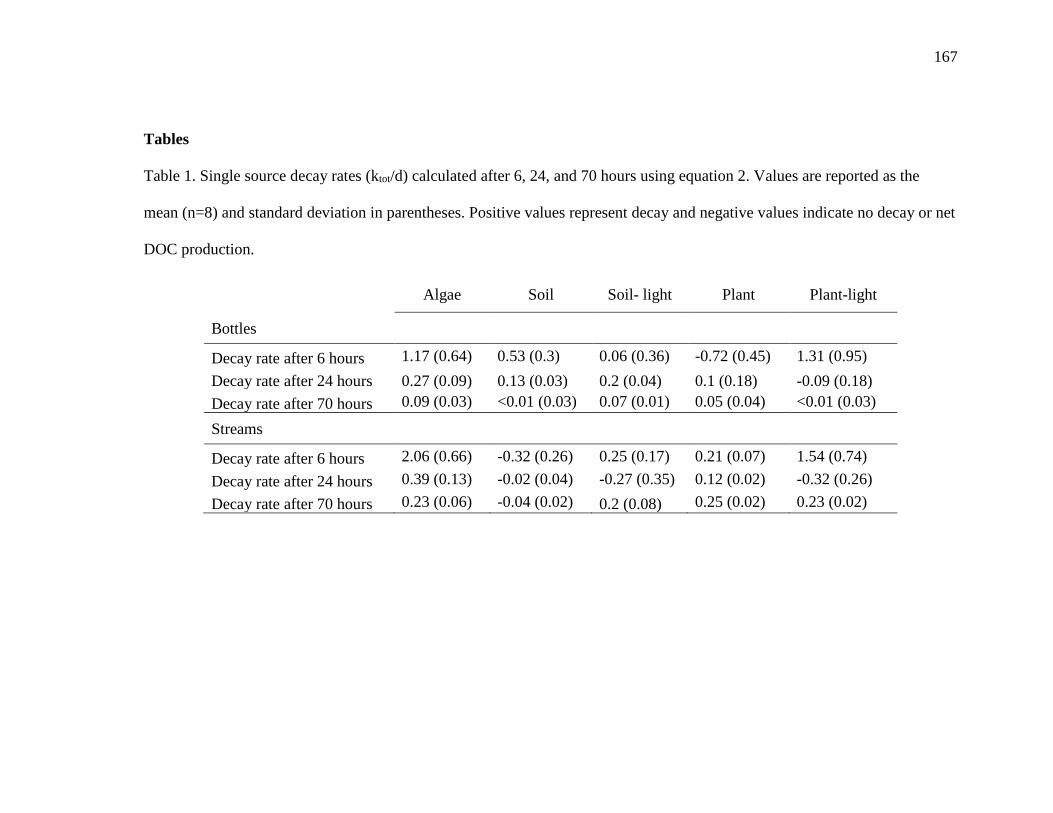
167
Tables
Table 1. Single source decay rates (ktot/d) calculated after 6, 24, and 70 hours using equation 2. Values are reported as the
mean (n=8) and standard deviation in parentheses. Positive values represent decay and negative values indicate no decay or net
DOC production.
Algae Soil Soil- light Plant Plant-light
Bottles
Decay rate after 6 hours 1.17 (0.64) 0.53 (0.3) 0.06 (0.36) -0.72 (0.45) 1.31 (0.95)
Decay rate after 24 hours 0.27 (0.09) 0.13 (0.03) 0.2 (0.04) 0.1 (0.18) -0.09 (0.18)
Decay rate after 70 hours 0.09 (0.03) <0.01 (0.03) 0.07 (0.01) 0.05 (0.04) <0.01 (0.03)
Streams
Decay rate after 6 hours 2.06 (0.66) -0.32 (0.26) 0.25 (0.17) 0.21 (0.07) 1.54 (0.74)
Decay rate after 24 hours 0.39 (0.13) -0.02 (0.04) -0.27 (0.35) 0.12 (0.02) -0.32 (0.26)
Decay rate after 70 hours 0.23 (0.06) -0.04 (0.02) 0.2 (0.08) 0.25 (0.02) 0.23 (0.02)

168
Table 2. Descriptions of 5 components identified by PARAFAC and references that had a
tucker’s congruency coefficient of 0.95 or more for previously identified fluorophores in
the OpenFluor library (Murphy et al. 2014).
Excitation
emission
(nm)
References Reference description This study
description
C1 ex 340
em 435-440
Osburn et al 2011;
Stedmon et al 2007 Humic-like Humic-like
C2 ex 255-260
em 495-500
Walker 2009,
Yamashita et al 2008 Humic-like
Humic-like,
susceptible to
light degradation
C3 ex 248
em 430-440
Shutova et al 2014;
Osburn et al 2016 Humic-like
Humic-like,
product of light
degradation
C4 ex 315
em 385-390
Osburn et al 2011;
Shutova et al 2014
Recently derived or
microbial-derived
Recently derived,
terrestrial
C5 ex 278
em 330-335
Coble et al 1996;
Yamashita and
Tanoue 2003
Protein-like,
tryptophan-like Protein-like

169
Table 3. Estimated decay rates (1/d) for the labile, 𝑘𝑓𝑎𝑠𝑡 and semi-labile, 𝑘𝑠𝑙𝑜𝑤 pools of DOM in the prime-algae and prime-
light experiment at 6, 24 and 70 hours. Biexponential models were fit using equation 2 and biphasic models were fit using
equations 3 and 4. Model fit was assessed through linear regression of measured versus modeled final DOC concentrations
(Supplement 9). The high density interval (HDI) of effect-size was calculated as the difference in the HDI of the posterior
probability distribution of 𝑘𝑠𝑙𝑜𝑤and 𝑘𝑝𝑙𝑎𝑛𝑡 where a positive median effect size indicated a positive non-additive (priming)
effect.
t Model 𝑘𝑠𝑙𝑜𝑤 𝑘𝑓𝑎𝑠𝑡 Model fit Effect size
Hours mean (1/d), mean
(1/d), slope, r2 2.50% 50% 97.50%
Prime-Algae 6 Biexponential 1.25, 2.88 -1.23, 0.31 0.36, '0.94 -1.835 -1.459 -0.887 24 Biexponential 1.73, 1.89 0.06, 0.15 0.11, '0.61 -0.258 -0.068 0.235 70 Biexponential 2.55, 2.14 0.12, 0.05 0.13, 0.95 -0.180 -0.136 -0.037 70 Biphasic fixed = 0.31 0.28, 0.06 0.43, 0.88 -0.041 0.032 0.134
Prime-Light 6 Biexponential 3.19, 2.67 5.37, 2.18 0.20, 0.56 1.655 4.931 9.871 24 Biexponential 2.68, 2.32 4.52, 3.96 0.42, 0.13 -4.252 4.634 11.702
24 Biphasic fixed = 2.0 1.05, 0.96 0.55, 0.83 -0.764 0.880 2.990
a 𝑘𝑓𝑎𝑠𝑡 was fixed at 0.31 /d which was estimated from time zero to the breakpoint at 0.5 days using equation 3.
b 𝑘𝑓𝑎𝑠𝑡 was fixed at 2.0 /d which was estimated from time zero to the breakpoint at 0.25 days using equation 3.

170
Figures
Figure 1. Eight experimental streams and 8 bottle-bioassays were used to compare decay
in bioassays versus experimental streams and test the hypothesis labile DOM would
increase the decay rate of semi-labile DOM. Streams were in a greenhouse; half of
streams were covered with cardboard for the dark treatment (4 replicates), and half were
not for the light treatment (4 replicates; see picture of light treatments). Seven, 3-day
experiments were conducted as, 5 single-source experiments and 2 priming experiments.

171
Figure 2. Light streams (n=4) had significantly higher fluorescence index (FI) values than
dark streams (n=4) and all streams had higher FI values than bottles (n=8). SUVA was
not significantly different among bottles and streams. Letters indicate treatments that
differed by average FI or SUVA values. High FI values indicated more microbial derived
DOM and high SUVA values represented greater aromatic content of DOM.

172
Figure 3. Percent fluorescence contribution compared among components 1 through 5
(C1, C2, C3, C4, C5) after 1, 24 hours and 70 hours. Black lines represent dark streams;
dashed lines represent light streams. C1, C2 and C3 were humic-like, C4 was recently
derived humic-like, and C5 was protein-like (Table 2). All components were significantly
different by treatment, except C2 which had an interactive effect between dark (n=4) and
light streams (n=4).

173
Figure 4. Dissolved organic carbon (DOC) decay rates for bioassays, experimental
streams, and natural streams. Bottles include decay rate constants calculated for DOM
leachates from this study and Hotchkiss et al. 2015. Experimental streams values are
from this study, and streams values were calculated from modeled decay rates for real
streams (Griffiths et al. 2009, Epstein et al. 2016, Hall et al. 2016).

174
Figure 5. Average bioavailable DOC (BDOC) was significantly greater for experimental
streams compared to bottles across all experiments except soil, which had significantly
higher BDOC in bottles compared to experimental streams, and there were no other
significant differences among experiments. Boxes represent the median and interquartile
range, whiskers represent 2.5 and 97.5, and dots are outliers.

175
Supplement
Supplement 1. Text file of R code for biexponential and biphasic models.
### Biexponential model ###
modelString = "
model {
for ( i in 1:Ntotal ) {
y[i] ~ dt(mu[i], 1/sigma^2, nu)
mu[i] <- pr1*C1*exp(k1[s[i]]*x[i]) + pr2*C2*exp(k2[s[i]]*x[i])
}
for ( j in 1:Nsubj ) {
k1[j] ~ dnorm( k1mu , 1/(k1sigma)^2)
k2[j] ~ dnorm( k2mu , 1/(k2sigma)^2 )
}
# Priors
k1mu ~ dnorm( -1.57, 0.05 )
k2mu ~ dnorm( -0.21,0.05 )
sigma ~ dgamma( 1 , 0.05 )
k1sigma ~ dgamma( 1 , 0.05 )
k2sigma ~ dgamma( 1 , 0.05 )
nu ~ dexp(1/30.0)
}
### Biphasic model ###
modelString = "
model {
for ( i in 1:Ntotal ) {
y[i] ~ dt(mu[i], 1/sigma^2, nu)
mu[i] <- Co*exp(k1[s[i]]*tp)*exp(k2[s[i]]*(x[i]-tp))
}
for ( j in 1:Nsubj ) {
k1[j] ~ dnorm( k1mu , 1/(k1sigma)^2)
k2[j] ~ dnorm( k2mu , 1/(k2sigma)^2 )
}
# Priors
k1mu ~ dnorm( -2, 0.5 )
k2mu ~ dnorm( -0.21, 0.05 )
sigma ~ dgamma( 1 , 0.05 )
k1sigma ~ dgamma( 1 , 0.05 )
k2sigma ~ dgamma( 1 , 0.05 )
nu ~ dexp(1/30.0)
}

176
Supplement 2. References and values used to create figure 4. Depth and velocity are for
the stream or experimental stream DOM was collected from.
Reference DOM source Stream Assay
Decay (1/d)
Depth (m)
Velocity (m/s)
Epstein et al 2016 Natural Stream 0.6 1.04 0.36
Epstein et al 2016 Natural Stream 1.6 0.57 1.22
Epstein et al 2016 Natural Stream 2 0.7 0.86
Griffiths et al 2012 Natural Stream 0.001 - -
Griffiths et al 2012 Natural Stream 0.002 - -
Griffiths et al 2012 Natural Stream 0.002 - -
Griffiths et al 2012 Natural Stream 0.002 - -
Griffiths et al 2012 Natural Stream 0.003 - -
Griffiths et al 2012 Natural Stream 0.004 - -
Griffiths et al 2012 Natural Stream 0.007 - -
Griffiths et al 2012 Natural Stream 0.008 - -
Griffiths et al 2012 Natural Stream 0.009 - -
Griffiths et al 2012 Natural Stream 0.01 - -
Griffiths et al 2012 Natural Stream 0.013 - -
Griffiths et al 2012 Natural Stream 0.019 - -
Hall et al 2016 Natural Stream 0.041 1.3 0.57
Hall et al 2016 Natural Stream 0.045 1.3 0.39
Hall et al 2016 Natural Stream 0.048 1 0.45
Hall et al 2016 Natural Stream 0.109 0.6 0.53
Hall et al 2016 Natural Stream 0.258 1.1 0.49
Hall et al 2016 Natural Stream 0.337 1 0.98
Hall et al 2016 Natural Stream 0.416 1.4 0.52
Hall et al 2016 Natural Stream 0.495 0.6 0.59
Hall et al 2016 Natural Stream 0.819 0.8 0.36
Hotchkiss et al 2014 Algae Bioassay 0.038 0.6 0.59
Hotchkiss et al 2014 Algae Bioassay 0.074 0.8 0.36
Hotchkiss et al 2014 Algae Bioassay 0.075 1.1 0.49
Hotchkiss et al 2014 Algae Bioassay 0.092 1.2 0.43
Hotchkiss et al 2014 Algae Bioassay 0.098 1.4 0.52
Hotchkiss et al 2014 Soil Bioassay 0.001 1.1 0.49
Hotchkiss et al 2014 Soil Bioassay 0.004 0.8 0.36
Hotchkiss et al 2014 Soil Bioassay 0.011 1 0.45
Hotchkiss et al 2014 Soil Bioassay 0.017 1 0.98
Hotchkiss et al 2014 Soil Bioassay 0.023 1.4 0.52
Hotchkiss et al 2014 Soil Bioassay 0.024 0.6 0.59
Hotchkiss et al 2014 Soil Bioassay 0.024 1.2 0.43
Hotchkiss et al 2014 Soil Bioassay 0.026 1.3 0.39

177
Hotchkiss et al 2014 Soil Bioassay 0.052 1.3 0.57
Hotchkiss et al 2014 Soil Bioassay 0.058 0.6 0.53
This study Algae - 24 hr Stream 0.39 0.07 -
This study Algae - 6 hr Stream 2.06 0.07 0.6
This study Algae - 70 hr Stream 0.234 0.07 -
This study Algae -24 hr Bioassay 0.27 0.07 -
This study Algae -6 hr Bioassay 1.18 0.07 0.6
This study Algae -70 hr Bioassay 0.088 0.07 -
This study Light-plant - 6 hr Bioassay 1.31 0.07 0.6
This study Light-plant - 6 hr Stream 1.53 0.07 0.6
This study Light-plant - 70 hr Stream 0.225 0.07 -
This study Light-soil - 24 hr Bioassay 0.2 0.07 -
This study Light-soil - 6 hr Bioassay 0.06 0.07 0.6
This study Light-soil - 70 hr Bioassay 0.074 0.07 -
This study Light-soil - 70 hr Stream 0.202 0.07 -
This study Plant - 24 hr Stream 0.12 0.07 -
This study Plant - 6 hr Stream 0.21 0.07 0.6
This study Plant - 70 hr Stream 0.25 0.07 -
This study Plant-24 hr Bioassay 0.1 0.07 -
This study Plant-70 hr Bioassay 0.048 0.07 -
This study Soil - 24 hr Bioassay 0.13 0.07 -
This study Soil - 6 hr Bioassay 0.54 0.07 0.6
This study Soil - 70 hr Bioassay 0.014 0.07 -

178
Supplement 3. Benthic biomass measured as ash free dry mass (AFDM) and chlorophyll
a (Chla) for each experiment. Boxplots represent the average concentration per area of
AFDM and Chla for 3 samples collected during each experiment from each stream.
Concentration of each variable was multiplied by the total volume of slurry produced
from scrubbing the cobble and normalized by the area of the cobble.

179
Supplement 4. High density intervals (HDI) of the difference between labile (algae, soil-
light, plant-light) and semi-labile (soil, plant) decay rate HDIs. A positive median
difference in decay rate indicated a significant difference in decay rate constants (bold)
estimated by the single-source model (Eqn. 2).
Algae-Soil Algae-Plant
Streams 2.5% 50% 97.5% 2.5% 50% 97.5%
6 hours 0.75 1.18 1.60 0.25 0.90 1.53
24 hours 0.08 0.20 0.29 -0.03 0.13 0.25
70 hours -0.09 0.05 0.15 -0.18 -0.07 0.02
Bottle
6 hours --0.05 0.30 0.66 0.76 0.94 1.14
24 hours -0.03 0.06 0.12 0.28 0.13 -0.02
70 hours 0.00 0.03 0.05 0.09 0.05 0.02
Plant-light-Soil Plant-light-Plant
Streams 2.5% 50% 97.5% 2.5% 50% 97.5%
6 hours 0.39 0.90 1.43 -0.11 0.62 1.36
24 hours -0.39 -0.16 0.06 -0.50 -0.23 0.02
70 hours 0.00 0.00 0.00 -0.09 -0.11 -0.12
Bottle
6 hours -0.31 0.36 1.02 0.50 0.99 1.51
24 hours -0.18 -0.12 -0.07 0.13 -0.05 -0.21
70 hours -0.10 -0.05 -0.02 0.00 -0.03 -0.05
Soil-light-Soil Soil-light-Plant
Streams 2.5% 50% 97.5% 2.5% 50% 97.5%
6 hours -0.17 1.45 3.21 -0.67 1.17 3.13
24 hours -0.75 -0.20 0.17 -0.86 -0.28 0.12
70 hours -0.19 0.05 0.15 -0.28 -0.07 0.03
Bottle
6 hours -0.30 -0.24 -0.17 0.50 0.39 0.31
24 hours 0.02 0.03 0.04 -0.10 0.10 0.33
70 hours 0.00 0.01 0.02 -0.01 0.03 0.10

180
Supplement 5. Comparison of decay rates calculated over 6 hours for light and dark
streams.

181
Supplement 6.1. Differences in the BIX, HIX, FI and SUVA between treatments. Letters
at the top of panels represent results of the Tukey HSD test.

182
Supplement 6.2. Bayes factor results for 5 linear models that described variation in fluorescence indices. The biological index
(BIX), the humification index (HIX), the fluorescence index (FI), the peak T to peak C ratio (TC) and SUVA at absorbance
wavelength 254 nm (SUVA), were compared after 70 hours in each experiment. Linear models were also fit using the percent
contribution of each component from the PARAFAC model (C1-C5). The higher the Bayes Factor the better the model
explained variation in the dependent variable. Bold cells are the highest Bayes Factor in each row.
Treatment Treatment +
Bottle/Stream
Treatment +
Bottle/Stream
+ interaction
Treatment +
Dark/Light/Bottleb
Treatment +
Dark/Light/Bottlea +
interaction
BIX 2.1 E 44 0.3 0.3 0.2 0.1
HIX 3.3 E 31 4.4 1.5 E 3 1.9 2.5 E 4
FI 1.6 E 19 1.5 E 11 9.6 E 11 3.7 E 25 1.5 E 30
TC 9.7 E 8 1.2 0.55 0.8 1.1
SUVA 7.6 E 31 1.3 E 14 1.2 E 17 2.5 E 47 2.5 E 49
Percent C1 1.6 E 27 22.6 2.2 E 3 29.6 1.7 E 3
Percent C2 4.4 E 15 4.5 E 8 6.1 E 9 6.6 E 17 2.7 E 20
Percent C3 1.2 E 51 3.4E 2 3.5 E 13 6.1 E 4 2.2 E 21
Percent C4 2.4 E 70 61.3 4.6 E 9 38.1 4.4 E 10
Percent C5 7.7 E 10 4.5 21.2 3.1 8.7

183
Supplement 7. Spectral characteristics of five components resolved by PARAFAC.
Fluorescence intensities are in Raman units (top). Ex = excitation and Em = emission
wavelengths. Split-half validation of reverse normalized model that produced
components 1 to 5 (bottom).

184
Supplement 8. Pearson’s correlations between components and fluorescence indices. All
fluorescence samples were included.

185
Supplement 9.1. Left panels are modeled biexponential DOC decay (red) and actual DOC
decay (black) for the prime algae experiment after 70, 24, and 6 hours. Right panels are
the modeled data points in black and the modeled versus actual 1:1 line in red.
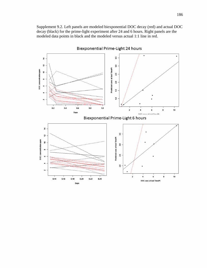
186
Supplement 9.2. Left panels are modeled biexponential DOC decay (red) and actual DOC
decay (black) for the prime-light experiment after 24 and 6 hours. Right panels are the
modeled data points in black and the modeled versus actual 1:1 line in red.

187
Supplement 9.3. Left panels are modeled biphasic DOC decay (red) and actual DOC
decay (black) for the prime-algae experiment (top) and prime-light experiment (bottom).
Right panels are the modeled data points in black and the modeled versus actual 1:1 line
in red.

188
Supplement 10. Bioavailable DOC (BDOC) in the single-source plant experiment and the
2 priming experiments. More BDOC in priming experiments than in the plant experiment
would indicate a possible positive non-additive effect. While BDOC was higher in the
streams of the prime-light experiment there was not significant difference across
treatments (ANOVA F = 0.94, p = 0.46).

189
CONCLUSIONS
Despite the difficulty in distinguishing sources of OM in watersheds with mixed
land use, I identified major sources of OM to the Jordan River including WWTP effluent,
OM derived from Utah Lake, and autochthonous and terrestrial sources. WWTP effluent
OM sources were incorporated into FPOM in the Jordan River and had increased
influence on FPOM during low flow periods in fall. There were also increased
autochthonous sources of CPOM in spring and summer. These results support the
hypothesis outlined in the Urban Watershed Continuum (Kaushal and Belt 2012) that
urbanization can increase the proportion of autochthonous sources of OM and in effect,
replace terrestrial OM with more labile sources of OM.
I did not identify any land cover metrics that correlated with OM source or
composition across multiple watersheds. The greatest differences in OM were due to the
influence of WWTP effluent, OM sources from Utah Lake, and human activity within
federally designated national forests. None of these human activities were accounted for
in land cover categories of the National Land Cover Dataset. Further study is needed to
understand the influence of landcover on OM source and composition, especially in arid
regions which have different flow regimes than temperate systems, and are influenced by
large lakes and reservoirs within multiple land cover types. While some previous studies
have specifically compared WWTP OM to other OM sources within the landscape
(Wassenaar et al. 2010, Gucker et al. 2011, Duan et al. 2014), I think more OM studies
conducted in watersheds with wastewater effluent should directly incorporate OM
samples from WWTPs into their sampling regimes. Likewise, researchers of wastewater
treatment engineering and biogeochemistry are disconnected from sociology, biology and

190
ecology researchers, areas of study that all inform watershed management. Increased
collaboration across disciplines could rapidly advance our understanding of the sources
and composition of OM within a matrix of land cover, and the ecological impacts of
differences in land cover on rivers.
It is important to identify and quantify the sources and lability of OM in rivers to
inform management decisions aimed at OM load and associated pollutant reduction.
Here, I outline how OM source identification can help reduce OM loads of either
autochthonous or terrestrial sources. Possible strategies to reduce terrestrial OM loads
include geomorphic alterations of riparian and benthic habitat to increase OM retention
time within a reach. Greater habitat heterogeneity through the addition of bio swales,
large benthic substrates (e.g. boulders), and wood additions may increase OM retention
and/or reduce benthic embeddedness, consequently increasing hyporheic exchange
(Hester and Gooseff 2010). Greater retention and hyporheic exchange increase the
amount of habitat and time available for microbial OM processing, thereby reducing OM
export from a reach (Wollheim et al. 2018). However, geomorphic alterations should be
considered with extreme caution because reach-scale restoration studies suggest they are
not effective at improving ecosystem function (Bernhardt and Palmer 2011).
To reduce autochthonous OM sources, effective reduction strategies must occur at
the multi-watershed scale. As is the case with the Jordan River, the primary source of
problematic OM is from Utah Lake, which receives water from 6 other major watersheds
(Psomas 2009). Reduced inorganic nutrients could reduce in-stream primary production.
Potential nutrient reduction strategies include updating stormwater infrastructure to
reduce urban and agricultural runoff during storms, and encouraging best management

191
practices when applying fertilizer in urban and agricultural areas (Parr et al. 2016). Other
possible, but costly, nutrient reduction strategies in urban watersheds are wastewater
treatment facility updates, such as upstream filtration for membrane treatment and UV
disinfection (Henderson et al. 2009).
However, replacing infrastructure is expensive, and changing human behavior is
hard. I think future research to reduce OM loads in the Great Salt Lake Basin should
focus on how reservoirs and diversions have altered the natural flow regime (Miller et al.
2018, Wurtsbaugh et al. 2017). A recent study identified consumptive use of water in the
Great Salt Lake Basin as the cause of reduced lake levels (Wurtsbaugh et al. 2017). This
implies that water available to dilute OM loads is lacking. A study to assess the effect of
reservoirs and diversions on river flow regimes before and after impoundment
installations could reveal alterations to organic matter source and transport dynamics. It is
not realistic to remove dams and diversions, but knowledge of the flow regimes prior to
impoundment could outline strategies to return portions of the watershed to their natural
flow regimes. Then, management strategies could be specifically tailored to flow regimes
and problematic OM for each watershed. For example, if floodplain areas were lost,
perhaps constructed wetlands would help simulate ecological services provided by
floodplains.
In addition to knowledge of source identity and quantity, understanding OM
bioavailability can directly inform regional and global models of organic carbon cycling
(Cole et al. 2007, Raymond et al. 2013). Decay rates for terrestrial sources of DOM span
10 orders of magnitude due to variation in OM substrate, and methods used to quantify
dissolved organic carbon uptake (Cory and Kaplan 2012, Mineau et al. 2016). Likewise,

192
microbial transformation rates of labile DOM sources, especially naturally derived labile
DOM, are poorly constrained. Uncertainty of DOM transformation rates, combined with
unknown proportions of labile OM within the DOM pool, has limited robust estimates of
inorganic carbon evasion to the atmosphere from rivers (Wollheim et al. 2015).
Autochthonous and terrestrially derived DOM decay rates from this study can
inform future studies that aim to constrain OM transformation rates in rivers. DOM
reactivity and removal from rivers has been described as moderate (Wollheim et al. 2015)
to high (Hall et al. 2016). Uncertainty of DOM removal rates is derived from the portion
of the DOM pool for which removal is measured. For example, removal rates are
calculated for the entire DOM pool (Hall et al. 2016 and references), the terrestrial
portion (Mineau et al. 2016), or fractions separated by molecular weight (Skully et al.
2004) or hydrophobicity (Wollheim et al. 2015). My results emphasize the need to better
quantify both fast and slow decaying OM pools in rivers. Many measures of OM decay
are based on bioassays which likely underestimate OM demand in rivers. Direct
measurements of known sources of DOM in an experimental setting can help define the
lability of DOM along a continuum of minutes to millennia.
I have highlighted that the study of OM source, composition, and quality can
inform both watershed management and the study of carbon cycling at the watershed
scale. The management implications I discussed focused on source identification of OM
loads such as labile versus semi-labile sources of autochthonous, anthropogenic, or
terrestrial inputs. It is important to note these are water quality issues largely faced by
developed nations that have wastewater treatment infrastructure, while many developing
nations do not treat wastewater. I also believe estimates of OM demand for

193
autochthonous and terrestrial DOM from this study may inform models of OM
transformation and carbon dioxide evasion to the atmosphere. But, I emphasize that
further study is needed to standardize metrics and definitions of OM demand across
disciplines, and to identify measures of anthropogenic influence within watersheds that
can predict OM composition at a specified spatial scale.
194
Literature Cited
Bernhardt, E. S., and M. A. Palmer. 2011. River restoration: the fuzzy logic of repairing
reaches to reverse catchment scale degradation. Ecological applications 21:1926-1931.
Cole, J. J., Y. T. Prairie, N. F. Caraco, W. H. McDowell, L. J. Tranvik, R. G. Striegl, C.
M. Duarte, P. Kortelainen, J. A. Downing, and J. J. Middelburg. 2007. Plumbing the
global carbon cycle: integrating inland waters into the terrestrial carbon budget.
Ecosystems 10:172-185.
Cory, R. M., and L. A. Kaplan. 2012. Biological lability of streamwater fluorescent
dissolved organic matter. Limnology and Oceanography 57:1347-1360.
Duan, S., R. M. Amon, and R. L. Brinkmeyer. 2014. Tracing sources of organic matter in
adjacent urban streams having different degrees of channel modification. Science of the
Total Environment 485:252-262.
Gücker, B., M. Brauns, A. G. Solimini, M. Voss, N. Walz, and M. T. Pusch. 2011. Urban
stressors alter the trophic basis of secondary production in an agricultural stream.
Canadian Journal of Fisheries and Aquatic Sciences 68:74-88.
Hester, E. T., and M. N. Gooseff. 2010. Moving beyond the banks: hyporheic restoration
is fundamental to restoring ecological services and functions of streams. Environmental
Science and Technology 44:1521-1525.
Henderson, R. K., A. Baker, K. Murphy, A. Hambly, R. Stuetz, and S. Khan. 2009.
Fluorescence as a potential monitoring tool for recycled water systems: a review. Water
research 43:863-881.
Kaushal, S. S., and K. T. Belt. 2012. The urban watershed continuum: evolving spatial
and temporal dimensions. Urban Ecosystems 15:409-435.
Miller, M. P., D. M. Carlisle, D. M. Wolock, and M. Wieczorek. 2018. A database of
natural monthly streamflow estimates from 1950 to 2015 for the conterminous united
states. Journal of the American Water Resources Association.
Mineau, M. M., W. M. Wollheim, I. Buffam, S. E. Findlay, R. O. Hall, E. R. Hotchkiss,
L. E. Koenig, W. H. McDowell, and T. B. Parr. 2016. Dissolved organic carbon uptake in
streams: A review and assessment of reach‐scale measurements. Journal of Geophysical
Research: Biogeosciences 121:2019-2029.
Psomas Consulting. 2009. Utah Lake TMDL: pollutant loading assessment & designated
beneficial use impairment assessment. Utah Division of Water Quality.

195
Raymond, P. A., J. Hartmann, R. Lauerwald, S. Sobek, C. McDonald, M. Hoover, D.
Butman, R. Striegl, E. Mayorga, and C. Humborg. 2013. Global carbon dioxide
emissions from inland waters. Nature 503:355-359.
Scully, N. M., N. Maie, S. K. Dailey, J. N. Boyer, R. D. Jones, and R. Jaffé. 2004. Early diagenesis of plant‐derived
dissolved organic matter along a wetland, mangrove, estuary ecotone. Limnology and oceanography
49:1667-1678.
Wassenaar, L., J. Venkiteswaran, S. Schiff, and G. Koehler. 2010. Aquatic community
metabolism response to municipal effluent inputs in rivers quantified using diel 18O
values of dissolved oxygen. Canadian Journal of Fisheries and Aquatic Sciences 67:1232-
1246.
Wollheim, W., R. Stewart, G. R. Aiken, K. D. Butler, N. B. Morse, and J. Salisbury.
2015. Removal of terrestrial DOC in aquatic ecosystems of a temperate river network.
Geophysical Research Letters 42:6671-6679.
Wollheim, W., S. Bernal, D. Burns, J. Czuba, C. Driscoll, A. Hansen, R. Hensley, J.
Hosen, S. Inamdar, and S. Kaushal. 2018. River network saturation concept: factors
influencing the balance of biogeochemical supply and demand of river networks.
Biogeochemistry: doi:10.1007/s10533-018-0488-0.
Wurtsbaugh, W. A., C. Miller, S. E. Null, R. J. DeRose, P. Wilcock, M. Hahnenberger, F.
Howe, and J. Moore. 2017. Decline of the world's saline lakes. Nature Geoscience
10:816.
196
JULIE KELSO
Utah State University, Department of Biology, Ph.D. Ecology
juliekelso.weebly.com
EDUCATION
Utah State University, Logan, UT - Ph.D., Biology and Ecology
2013 - present
University of Central Arkansas, Conway, AR - M.S. Biology
2010 - 2012
Tulane University, New Orleans, LA - B.A. Environmental Policy
2002 - 2005
RESEARCH AND RELATED EXPERIENCE
Research and Teaching - Utah State University, Logan, UT……………Jan-13 to Dec 18
• Collected and analyzed water quality metrics of the Jordan River to for the Utah
Division of Water Quality to develop recommendations for Total Maximum Daily
Load allocations of phosphorus and organic matter
• Developed research questions and managed all water quality data collected for the
NSF funded project, iUTAH – innovative Urban Transitions and Aridregion
Hydro-sustainability
• Responsibilities included sampling of surface waters for nutrients and other water
quality constituents, QA-QC of water quality data for iUTAH database,
maintenance and sample analysis of Shimadzu carbon and total dissolved nitrogen
analyzer and Aqualog spectrofluorometer
• Teaching assistant for human anatomy, elementary microbiology, and
introductory biology
Science Reporter - Utah Public Radio, Logan, UT……………………...Jan-17 to Dec-17
• Researched, wrote, recorded, mixed audio and published online content for
weekly news segment on science related topics in Utah
• Feature writer on issues related to global climate change and water
Research and Teaching - University Central Arkansas, Conway, AR….Aug-10 to Dec-12
• Monitored macroinvertebrate communities in 17 streams in north central
Arkansas for potential effects of natural gas drilling
• Installed and maintained photo-monitored gages in 6 stream reaches to
characterize intermittent stream hydrology
• Compiled and analyzed macroinvertebrate density and biomass data for 3-year
sampling effort
• Collected storm samples of total and volatile suspended solids from siphon
samplers
• Teaching assistant for non-majors biology lab

197
PROFESSIONAL EXPERIENCE
Biological Technician
Wildlife Conservation Society, Prudhoe Bay, AK……………………….Apr-10 to Jun-10
• Banded migrating shorebirds for research investigating the effect of gas drilling
on nest predation
• Assisted with game camera monitoring of nest predators
Assistant Outreach Coordinator
Alliance for the Great Lakes, Chicago, IL……………………………….Apr-08 to Sep-08
• Helped recruit and coordinate volunteers in Illinois and Indiana for annual Great
Lakes beach cleanup in collaboration with the Ocean Conservancy’s
international beach cleanup day
• Organized and conducted three team leadership trainings for principal
volunteers
• Maintained an online database to track volunteers and citizen science data
• Promoted event to media outlets including web, radio, print, and television
Noxious Weed Inventory Intern
U.S. Forest Service, Salmon, ID………………………………………..May-06 to Nov-06
• Inventoried wilderness sites for US Forest Service noxious week inventory
program
• Used ESRI ArcPad and GIS to document and map noxious weed sites.
Fisheries Intern
U.S. Army Corps of Engineers, Bonneville Lock and Dam, OR Feb-06 to May-06
• Monitored sea lion predation of fishes from Bonneville Dam
• Identified predated fishes including shad, lamprey, Chinook, or Steelhead
Wildland Fire Prevention Intern
Bureau of Indian Affairs, Cloquet, MN Jun-05 to Nov-05
• Assessed over 1000 homes for risk to wildland fire on the Fond du Lac
Reservation
• Developed and implemented wildland fire prevention curriculum for grades K-5
PUBLICATIONS
Austin, J.B., J. E. Kelso, M. A. Evans-White, S.A. Entrekin. 2018. Can high volume
hydraulic fracturing effects be detected in large watersheds? A case study of the South
Fork Little Red River. Current Opinion in Environmental Sciences & Health.
DOI:10.1016/j.coesh.2018.04.003
Kelso, J.E. and S.A. Entrekin. 2017. Intermittent and perennial macroinvertebrate
communities had similar richness but differed in species trait composition depending on
flow duration. Hydrobiologia. DOI:10.1007/s10750-017-3393

198
Epstein, D.M., J.E. Kelso, and M.A. Baker. 2016. Beyond the urban stream syndrome:
Organic matter budgets for diagnostics and restoration of an impaired urban river. Urban
Ecosystems. 19:1041-1061. DOI:10.1007/s11252-016-0556
Kelso, J.E. and M.A. Baker. 2015. Filtering with a drill pump: an efficient method to
collect suspended sediment and filtrate. Journal of American Water Resources
Association. 52:1536-1541. DOI:10.1111/1752-1688.12368
PUBLISHED DATASETS
Kelso, J., M.A. Baker (2017). Dissolved organic matter spectrofluorometric properties
along a mountain to urban gradient in North East Utah, HydroShare,
http://www.hydroshare.org/resource/7722d73be4b348a9ad874fe29086c1fb
Kelso, J., M.A. Baker (2017). FPOM and DOM isotope values, HydroShare,
http://www.hydroshare.org/resource/4eb5c9c871e34aa4ae6951ce6d15020d
PRESENTATIONS
Kelso, J., and M.A. Baker. Characterization of organic matter sources within a matrix of
land use in Northeast Utah. Ecological Society of America. August 2017.
Kelso, J., E.Rosi, and M.A. Baker. Light-degraded dissolved organic matter increased the
decay rate of terrestrial organic matter in experimental streams. Society for Freshwater
Science Meeting. June 2017.
Kelso, J., and M.A. Baker. Characterization of dissolved organic matter sources along a
mountain to urban gradient. Society for Freshwater Science Meeting. May 2016.
Kelso, J., D.M. Epstein, and M.A. Baker. Characterization of riverine organic matter in
an urban landscape. Society for Freshwater Science Meeting. May 2015.
Epstein, D.M., J. Kelso and M.A. Baker. Organic matter budget for an impacted urban
river stream. Society for Freshwater Science Meeting. May 2014.
Kelso, J., D.M. Epstein, and M.A. Baker. Characterization of sources of organic matter to
an urban river. Society for Freshwater Science Meeting. May 2014.
Kelso, J., D.M. Epstein, and M.A. Baker. Characterization of sources of organic matter
to the Jordan River, UT. Symposium on Urbanization and Stream Ecology. May 2014.
Musto, A., S.A. Entrekin, N. Jensen, J.E. Kelso, B. Haggard, C. Gallipeau, E. Inlander,
and L.Massey, The relationship between land disturbance and trace elements in streams
of north-central Arkansas. Society for Freshwater Science Meeting. May 2013.

199
Kelso, J.E. and S.A. Entrekin. Use of the hyporheic zone as refuge by macroinvertebrates
in an intermittent and perennial Ozark stream. Society for Freshwater Science Meeting.
May 2013.
Kelso, J.E. and S.A. Entrekin. Macroinvertebrate communities in intermittent and
perennial Ozark streams. Great Plains Limnology Association. October 2012.
Kelso, J.E., and S.A. Entrekin. Macroinvertebrate communities in intermittent and
perennial Ozark streams. Society for Freshwater Science Meeting. May 2012.
POSTERS
Kelso, J., M.A. Baker. Characterization of riverine organic matter within a matrix of land
use in northeast Utah. American Geophysical Union, December 2017.
Gabor, R., R.M. Smith, J.F. Shah, J.E. Kelso, M.A. Baker, P.D. Brooks. The urban
watershed as a transformer of dissolved organic matter chemistry. American Geophysical
Union, December 2017.
Kelso, J., D. Epstein, M.A. Baker. Light-degraded dissolved organic matter may have
increased the decay rate of terrestrial organic matter in experimental streams. Utah State
University, Spring Runoff Conference. March 2017.
Kelso, J., D. Epstein, M.A. Baker. Characterization of dissolved organic matter along a
mountain to urban gradient. Utah State University, Spring Runoff Conference. March
2016.
Capito, L.M., J.E. Kelso, M.A. Baker. Diving into Utah’s water with spectrofluorometry.
Utah State University, Undergraduate Research Symposium. December 2015.
Entrekin, S.A., B. Austin, J.E. Kelso, S. Polaskey, A. Musto, and M. Evans-White. Does
hydrology and activity from natural gas development interact to alter quality of
communities in small streams? Society for Freshwater Science Meeting. May 2015.
Butterfield, A., J.E. Kelso, M.A. Baker. Photodegradation of dissolved organic matter in
the Jordan River, UT. National Conference on Undergraduate Research, April 2015.
Kelso, J., D. Epstein, M.A. Baker. Spectrofluorometric and isotopic characterization of
organic matter along a gradient of urban land use. Utah State University, Spring Runoff
Conference. March 2015.
Kelso, J. and M.A. Baker. Characterization of sources of organic matter to an urban river.
Utah State University, Spring Runoff Conference. April 2014.
Kelso, J. and S.A. Entrekin. Macroinvertebrate community structure in intermittent and
perennial Ozark streams. UCA Student Research Symposium. April 2012.

200
Kelso, J. and S.A. Entrekin. Does refuge affect macroinvertebrate communities in
intermittent Ozark streams? Society for Freshwater Science Meeting. May 2011.
Kelso, J. and S.A. Entrekin. Refuge use by macroinvertebrates in intermittent Ozark
streams. University of Central Arkansas College of Natural Sciences
and Mathematics Symposium. April 2011.
STUDENT MENTORING
Lindsay Capito, Utah State University, Logan, Utah – 2015-2016
• Trained in analytical laboratory methods including spectrofluorometric analysis
of dissolved organic matter, chlorophyll a, isotope sample preparation, and
volatile suspended solids analysis
• Assisted with experiment at the Cary Institute of Ecosystem Studies
Experimental Stream Facility in July 2016
Simone Jackson, University of Utah, Salt Lake City – Summer 2015
• Trained to collect aquatic macroinvertebrates and periphyton for stable isotope
analysis
• Helped identify macroinvertebrates to family
• Helped summarize data for poster presented at the Society for Freshwater
Science meeting
Andrew Butterfield, Westminster College, Salt Lake City – Summer 2014
• Conducted an experiment on the Jordan River in which Andrew collected,
analyzed and presented results at the National Conference on Undergraduate
Research 2015
Chelsea Miller, Carolyn Pollard, David Hiltenbrand, Loren Biggs, University of Central
Arkansas – 2011-2012
• Trained and managed undergraduate student workers hired to sort and identify
macroinvertebrates and process organic matter biomass samples.
• Lead macroinvertebrate sampling field campaigns in headwater streams.
GUEST LECTURER
BIO 1010 Science for the Citizen, Ecosystem Ecology, April 21-24, 2016
BIO 2220 Ecology, Community Structure, November 7, 2017
GRANTS AND AWARDS
USU Student Association Enhancement Award Jan 2017 – $4,000
USU Dissertation Enhancement Award Jan 2016 – $10,000
USU Ecology Center Graduate Research Award, Apr 2015 – $3,700
Society for Freshwater Science, Mulholland Fund Research, Mar 2015 – $1000
USU Research and Graduate Studies Student Travel Award, Feb 2015 – $300
USU Ecology Center Graduate Research Award, Apr 2014 – $4000
Center for Woman and Gender Graduate Student Travel Award, Apr 2013 – $500

201
UCA University Research Council Student Research Grant, Sep 2011 – $800
Arkansas Game and Fish Conservation Scholarship, Jul 2011 – $1000
UCA Travel Award, Feb 2010 – $500
Outstanding Student Poster, Spring Runoff Conference, Logan, UT, Apr 2014
MEMBERSHIPS AND SERVICE
American Geophysical Union (2017-2018)
Biology Graduate Program Committee – Student representative (Jan 2014- Aug 2015)
USU Ecology Center Seminar Series Committee – (2013-2015)
American Water Works Association (2013-2014)
Society for Freshwater Science (2010 - present)
Merchandise Committee Chair – 2017 Annual Meeting
American Fisheries Society (2010-2012)
Ecofest Volunteer (2010-2012)
Annual public outreach event for city of Conway, AR
Backyard water quality sampling workshop, Clinton, AR – 2010
REVIEWER
Hydrobiologia
Science of the Total Environment
PROFESSIONAL DEVELOPMENT
Alan Alda Center for Communicating Science Workshop, Logan, UT, Oct 2016
Software Carpentry Workshop, Logan, UT, Mar 2015
Dissolved Organic Matter Fluorescence Workshop, Boulder, CO, Jul 2014
One-dimensional Transport with Inflow and Storage (OTIS) solute transport workshop,
Portland, OR, May 2014
Getting Started as a Successful Proposal Writer and Academician, Logan, UT, Feb 2013
Aquatic GIS Workshop, St. Louis, MO, Jun 2011
Wilderness First Aid, Salmon, ID, Jun 2006