oradea journal of business and...
TRANSCRIPT
1
University of Oradea Faculty of Economic Sciences Doctoral School of Economics
with the support of the Research Centre for Competitiveness and
Sustainable Development and Department of Economics
Oradea Journal of Business and Economics
Volume 2/2017, Issue 1
ISSN 2501-1596, ISSN-L 2501-1596

2
This page intentionally left blank.
EDITORIAL TEAM Editor-in-chief:
Daniel Bădulescu, PhD., University of Oradea, Faculty of Economic Sciences, Romania Associate Editors-in-chief:
Adriana Giurgiu, PhD., University of Oradea, Faculty of Economic Sciences, Romania, Alina Bădulescu, PhD., University of Oradea, Faculty of Economic Sciences, Romania, Executive editor:
Tomina Săveanu, PhD., University of Oradea, Faculty of Economic Sciences, Research Centre for Competitiveness and Sustainable Development, Romania Scientific and editorial board:
Nicolae Istudor, PhD., Bucharest University of Economic Studies, Faculty of Agri-Food and Environmental Economics, Romania Piero Mella, PhD., University of Pavia, Department of Economics and Management, Italy Mihai Berinde, PhD., University of Oradea, Faculty of Economic Sciences, Romania Xavier Galiegue, PhD., University of Orleans, Laboratory of Economics of Orleans, France Patrizia Gazzola, PhD., University of Insubria, Department of Economics, Italy Ruslan Pavlov, PhD., Central Economics and Mathematics Institute of the Russian Academy of Science, Russian Federation Gerardo Gomez, PhD., National University of Piura, Faculty of Accounting and Finance, Peru Christian Cancino, PhD., University of Chile, Faculty of Economics and Business, Chile Ion Popa, PhD., Bucharest University of Economic Studies, Faculty of Management, Romania Maria Chiara Demartini, PdD., University of Pavia, Department of Economics and Management, Italy Laura Cismas, PhD., West University of Timisoara, Faculty of Economics and Business Administration, Romania Gheorghe Hurduzeu, PhD., Bucharest University of Economic Studies, Faculty of International Business and Economics, Romania Mariana Golumbeanu, PhD., National Institute for Marine Research and Development “Grigore Antipa”, Romania Istvan Hoffman, PhD., Eötvös Loránd University (ELTE) Faculty of Law, Hungary
Ivo Zdahal, PhD., Mendel University in Brno, Faculty of Regional Development and International Studies, Czech Republic Valentin Hapenciuc, PhD., “Stefan cel Mare” University Suceava, Faculty of Economic Sciences and Public Administration, Romania, Zoran Čekerevac, PhD., “Union – Nikola Tesla” Belgarde University, Faculty of Business and Industrial Management, Republic of Serbia Emre Ozan Aksoz, PhD., Anadolu University, Faculty of Tourism, Turkey Nicolae Petria, PhD., University Lucian Blaga Sibiu, Faculty of Economic Sciences, Romania Olimpia Ban, PhD., University of Oradea, Faculty of Economic Sciences, Romania Ioana Teodora Meșter, PhD., University of Oradea, Faculty of Economic Sciences, Romania Adrian Florea, PhD., University of Oradea, Faculty of Economic Sciences, Romania Dorin Paul Bâc, PhD., University of Oradea, Faculty of Economic Sciences, Romania Adalberto Rangone, PhD., University of Pavia, Faculty of Business Administration, Italy Mariana Sehleanu, PhD., University of Oradea, Faculty of Economic Sciences, Romania Diana Perțicas, PhD., University of Oradea, Faculty of Economic Sciences, Romania Ramona Simuț, PhD., University of Oradea, Faculty of Economic Sciences, Romania Roxana Hatos, PhD., University of Oradea, Faculty of Economic Sciences, Research Center for Competitiveness and Sustainable Development, Romania
Oradea Journal of Business and Economics (OJBE) is an open access, peer-reviewed journal, publishing researches in all fields of business and economics. The Journal is published exclusively in English. It publishes two regular issues per year, in March and September, and occasionally one special issue, on a special theme (if case). Articles published are double-blind peer-reviewed and included into one of the following categories: theoretical and methodological studies, original research papers, case studies, research notes, book reviews. Volume 2, Issue 1, March 2017 ISSN 2501-1596 (in printed format). ISSN-L 2501-1596 (electronic format) Journal site: http://ojbe.steconomiceuoradea.ro/.
Acknowledgement Oradea Journal of Business and Economics wishes to acknowledge the following individuals for their assistance with the peer reviewing of manuscripts for this issue, translation and IT support, in on-line and print publishing, as well as international database indexing: Dr. Laurentiu Droj, Dr. Cornel Nicu Sabau, Adrian Nicula, Cătălin Zmole, Andrei Bădulescu. Their help and contributions in maintaining the quality of the journal are greatly appreciated.
Contents
Regular papers
Customer Satisfaction and Loyalty: A Study of Interrelationships and Effects in Nigerian
Domestic Airline Industry
Rahim A. Ganiyu…….………………………………………………………….……………..7
Can There Be a Competitor to Traditional Arable Crops in Romania?
Margit Csipkés…………………………………………………………………………………21
Using Wavelets in Economics. An Application on the Analysis of Wage-Price Relation
Vasile-Aurel Caus, Daniel Badulescu, Mircea Cristian Gherman ……………….……….32
The Link Between Bank Credit and Private Sector Investment in Nigeria from 1980-2014
Ephraim Ugwu, Johnson Okoh, Stella Mbah… …………………………………….………43
Papers selected from the Doctoral Symposyum 2016
The Structural Evolution of the Banking System in Romania under the Impact of FDI
Vasile Cocriş, Maria-Ramona Sârbu ……………………………………………….………55
Analysis of the Trinom Migration - FDI - Competitiveness. Case Study: Romania
(2004-2015)
Ana Maria Talmaciu (Banu), Laura-Mariana Cismaş…………………………………..…..63
The Price Evolution in the Context of Economic Crisis
Doriana Andreea Rămescu, Nicoleta Sîrghi………………………………………………..72
The Differences between Women Executives in Japan and Romania
Irina Roibu, Paula Alexandra Roibu (Crucianu)………..……………………………........81
Exploring the Obstacles and the Limits of Sustainable Development. A Theoretical Approach
Paula-Carmen Roșca ………………………………………………………………….…….91
Miscellaneous
The Doctoral Symposiyum - Oradea 2016: an overview ..................................................... 99

This page intentionally left blank.
Oradea Journal of Business and Economics, Volume II Issue 1 Published on March 2017
7
CUSTOMER SATISFACTION AND LOYALTY: A STUDY OF INTERRELATIONSHIPS AND EFFECTS IN NIGERIAN DOMESTIC AIRLINE INDUSTRY Rahim A. Ganiyu Department of Business Administration, University of Lagos, Lagos, Nigeria [email protected]
Abstract: The debate concerning the interrelationships and effects between customer satisfaction and loyalty has been tossed back and forth, without a consensus opinion. This study examines the linkages between customer satisfaction and loyalty in Nigerian domestic airline industry. The study adopted correlation research design to elicit information via questionnaire from 600 domestic air passengers drawn through convenience sampling technique. The data obtained from the respondents were analysed with Pearson correlation analysis, linear regression, and One-way analysis of variance. Based on 383 completed data, the results provide support for the association and influence of customer satisfaction on customer loyalty. The study also found out that frequent air travelers displayed more loyalty tendency towards airline carriers compared to non-frequent air passengers. On the basis of aforementioned findings, the study concludes that customer satisfaction is extremely important in building and enhancing customer loyalty. Therefore, airline carriers should implement strategies that will guarantee long-term relationship with air travellers by offering service quality that will meet and exceeds their expectations and by extension customer satisfaction. Keywords: customer satisfaction, loyalty, loyalty programme, service failure, domestic air travel, airline industry. JEL classification: M30, M31. 1. Background to the study Across the globe, the airline industry is a progressively growing segment of most economy and it has developed rapidly to become one of the most common means of travel. Specifically, airline industry facilitates economic development, world trade, tourism and global investment among other numerous benefits. Nonetheless, the importance of this industry is not only related with the combined significance of connectivity, but its contribution to the growth of numerous businesses which depend on airlines, such as hotels businesses, car hire operators, tourism etc. Currently, customer satisfaction with the service quality offered by airlines has become the most significant factor for success and survival in the airline industry. Customer satisfaction, according to Oliver (1997) is derived from the Latin word Satis (enough) and Facere (to do or make). In general, satisfaction is an internal view which offshoot from customers own experience of a consumption or service experience. Although the connection between customer satisfaction and company success has traditionally been tied to faith, and numerous satisfaction studies have supported this position (Hill and Alexander, 2000). Notwithstanding the aforementioned position, customer satisfaction has always been considered a vital business goal because of its crucial role in the formation of customer’s desire for future purchase or tendency to buy more (Mittal and Kamakura, 2001). Customer satisfaction, according to Pizam and Ellis (1999) refer to psychological notion that encompasses the feeling of comfort and pleasure that emanates from obtaining what one
Oradea Journal of Business and Economics, Volume II Issue 1 Published on March 2017
8
hopes for and expects. According to Kotler (2001: 58) “satisfaction is the feeling of pleasure or disappointment resulting from comparing the performance (or outcome) of a product or service perceived quality in relation to the buyer’s expectation”. However, in spite of the significance of customer satisfaction, many firms still experience a high level of customer switching despite been satisfied (Oliver, 1997; Taylor, 1998). This scenario has prompted a number of academics such as Jones and Sasser (1995), Reichheld (1996) and Egan (2004) to condemn the focus of attention on customer satisfaction and appeal for a paradigm shift to the pursuit of loyalty as a strategic business objective. No doubt, the quality of service offered to air passengers is crucial for enhancing customer satisfaction (Gilbert and Wong, 2003; Rahim, 2015). Likewise, customer satisfaction is pivotal to loyalty formation. For instance, Reichheld and Sasser (1990) discover that loyal customers are keen to (1) re-buy products despite attractive competitive alternatives that might propel them to try out competing products, (2) commit substantial amount of money on firm’s product line and service, (3) endorse and promote the firm’s goods or services to other customers, and (4) offer the firm truthful feedback as regards the performance of their products/services. According to Too, Souchon, and Thirkell (2001), loyalty refers to commitment to rebuy the favorite product or service in the future, despite situational and marketing efforts which can alter the behaviour. To a substantial number of researchers, loyalty is strongly connected to customer repeat patronage and retention (Too et al, 2001; Samaha, Palmatier and Dant, 2011). Statement of the problem Passengers loyalty is what all airlines seek, and retaining customers imply lesser costs (compared with that of attracting new ones), particularly in such a time of economic depression leading to declining demand for air transportation and increasingly competitive markets. No doubt, one of the most vital issues that have greater influence on loyalty formation is creating a good flight experience (quality of service). The inherent characteristics of airline services have lent themselves to a relationship marketing tactic, however, several customer-related approaches of airlines focus on customer loyalty initiatives which increase short-term sales instead of focusing on long-term quality relationships between the airline operators and air travellers (Bejou and Palmer, 1998). Therefore, for airline operators to balance their short-term and long-term business objectives, they must devise strategies to deliver their services more satisfactorily than their competitors (Nadiri, Hussain, Ekiz, and Erdogan, 2008; Rahim, 2016a). A remarkable service experience, no doubt will enhance customer satisfaction, builds positive emotions and customer loyalty towards the service provider. Rahim (2015) observes that perceived service quality of domestic airline operators in Nigeria has generally been adjudged to be poor; consequently, the level of passengers’ satisfaction and loyalty is low. However, to a dissatisfied air passengers’, the only available option is to switch to alternative airline as refund is impossible once the flight trip has been accomplished. The immediate consequence of this scenario is negative word of mouth communication from customers that experience bad flight experience and this will lead to a devastating effect such as loss of revenue, customer’s complaints etc. A review of extant literature related to airline industry revealed that the relationship between customer satisfaction and loyalty has generated a lot of debate and controversy. To date, the controversy is unsettled. Likewise, the claim that customer satisfaction leads to loyalty appears less convincing to many researchers (Rahim, Ignateous, and Adeoti, 2012; Egan, 2004; Pritchard and Silverstro, 2005). Similarly, some scholars have reported instances where despite improving customer satisfaction level, many firms still experience challenges in enhancing their profitability (Timothy, Bruce, Lerzan, Tor, and Jay, 2007; Tim, Lerzan, Alexander, and Luke, 2009). Despite the significance of the above-mentioned issues, researchers have paid scant attention regarding the subject matter in the context of the
Oradea Journal of Business and Economics, Volume II Issue 1 Published on March 2017
9
Nigerian airline industry. Against the aforementioned backdrops, this study seeks to achieve the following objectives: (1) to study the relationship between customer satisfaction and loyalty in Nigerian domestic airline industry, (2) to evaluate whether flight frequency is related to passengers loyalty in Nigerian domestic airline industry. Research hypotheses The following relationships were hypothesized.
1. There is no significant relationship between customer satisfaction and loyalty in Nigerian domestic airline industry.
2. Compared with infrequent travellers, frequent air passengers are not likely to display more loyalty tendency in Nigerian domestic airline industry.
2. Theoretical and literature review Confirmation and disconfirmation theory of satisfaction There are several theoretical approaches to explain the relationship between disconfirmation and dissatisfaction as the framework for customer satisfaction theory. Some of these approaches are variants of the consistency theories and they focus on the nature of the process of matching and comparing the consumer’s post-usage behaviour (Peyton, Pitts and Kamery, 2003). Foremost among these approaches are: the theory of assimilation, the theory of contrast, the theory of assimilation-contrast, the theory of negativity, and the theory of hypothesis testing. Adee (2004) maintains that numerous theories have been used to comprehend the process through which customers form satisfaction judgments. These theories according to him can be broadly classified under three groups: expectancy disconfirmation, equity, and attribution. Drawing on Helson (1964) adaptation level theory, Oliver (1977, 1980) develops expectation-disconfirmation paradigm (EDP) as a foundational theory for the assessment of customer satisfaction. The fundamental principle of EDP model is that, customer satisfaction is connected to the magnitude and direction of the disconfirmation experience (Oliver, 1980). According to Paterson (1993), disconfirmation represents the gap between consumer pre-purchase expectations and perceived performance of the product or service. Which suggests that consumers buying decision is contingent on prior expectations about the expected performance, which form the yardstick for evaluating product or service performance. Hence, if the assessment meets consumer prior expectation confirmation occurs which leads to satisfaction. On the other hand, disconfirmation arises where there is a discrepancy between expectations and performance which causes dissatisfaction (Oliver, 1997). Similar to the instance of SERVQUAL model, scholars have questioned the validity of the expectancy-disconfirmation model. Miller (1977) notes that customers elicited several different types of expectations (ideal, minimum, predicted, and normative performance), which may be problematic to comprehend and may explain significant variations in the strength of expectations relationship with other concepts in the satisfaction model. Another inadequacy of the EDP model is that post-purchase evaluations may not directly relate to original expectations, as such consumers may demonstrate satisfaction or dissatisfaction in some occasions where expectations never occurred (McGill and Iacobucci, 1992). Correspondingly, Iacobucci, Grayson, and Ostrom (1994) document another drawback of the EDP model which accentuates that customers will appraise a service favourably, as long as it meet or exceeds their expectations. Contrary to this claim, in a context where customers are manipulated to purchase a low-grade or less desirable brand due to scarcity of their preferred brand, then consumers may not automatically experience disconfirmation of a pre-experience assessment. Based on the aforementioned criticisms, a number of customer satisfaction theories have been advocated namely: value-precept theory,
Oradea Journal of Business and Economics, Volume II Issue 1 Published on March 2017
10
evaluative congruity model (or the social cognition model) among others to address the shortcomings of the EDP model. Towards a definition of customer satisfaction Customer satisfaction is a construct that has appeared in many fields of study and has been central to the marketing concept for several decades. The process of appraising customer expectations with the product or service’s performance is the heart of satisfaction development and this process has conventionally been labeled as the ‘confirmation/disconfirmation’ (Vavra, 1997). Thus, if perceived performance is less than expected, assimilation will occur, but if perceived performance varies from expectations significantly, contrast will occur, and the gap in the perceived performance will be inflated (Vavra, 1997). The performance of a company in terms of the quality of its product/services leads to customer satisfaction (Huang and Feng, 2009). Generally, satisfaction can be observed by subjective factors (i.e. customer needs, emotions) and objective factors (e.g. product and service attributes). By and large, satisfaction is an attitude molded by the customer to compare their pre-purchase expectations to their subjective perceptions of the performance of the product or service (Oliver, 1980). According to Yi (1990), customer satisfaction refers to collective outcome of perception, evaluation and the resulting psychological reactions to the consumption experience with a product/service. Chang, Wang, and Yang (2009) defined customer satisfaction as a psychological response or an evaluation of emotions from the customer. According to Garbarino and Johnson (1999) and Gronholdt, Martensen, Kristensen (2000), satisfaction is the outcome or assessment of what the customer initially expected and what they actually experienced during use and consumption of the product/service. Giese and Cote (2002) observe that there is no universal definition of customer satisfaction; hence, they view it as a recognised form of response (cognitive or affective) that relates to a particular context (e.g. a purchase experience and/or the related product) and arises at a certain time (i.e. post-purchase, post-consumption). Determinants of customer satisfaction Customer satisfaction has become a fundamental goal of all business organisations; this position is derived from long held conviction that for a firm to be profitable, it must satisfy customers (Shin and Elliott, 2001; Ranaweera and Prabhu, 2003). Generally, academics and business practitioners have long admitted that customer satisfaction is one of the highest priorities of business organizations and research have also shown that customer satisfaction is a key determinant in maintaining and sustaining business relationship (Oliver, 1997; Ahmad, 2007; Rahim, 2016b). Essentially, customer satisfaction is influenced by overall quality/price expectations (Anderson, 1994), firm’s image (Aga and Okan, 2007), and persons’ desires (Spreng, MacKenzie and Olshavsky, 1996). According to Oliver (1997), the determinants of customer satisfaction can be categorized into: instrumental factors (the performance of the physical product) and expressive factors (the psychological performance of the product). He later maintained that for customer’s to be satisfied, the product or service must meet expectations on both instrumental and expressive outcomes. Perspectives on customer loyalty The term “loyalty” has its direct philological origin in old French word, however, its older linguistic roots comes from the Latin word “Fidelis” (Stanford Encyclopedia of Philosophy, 2013). In service domain, loyalty has been conceptualized in an extensive form such as “observed behaviors”; these behavioural expressions according to Caruana (2002) relate to the brand not just thoughts. Largely, it is difficult to advance a universal definition of customer loyalty as it has been defined and measured in a myriad of ways too numerous for a single study to completely discuss. From a general viewpoint, loyalty can be described as
Oradea Journal of Business and Economics, Volume II Issue 1 Published on March 2017
11
the response consumer’s exhibit to brands, services, stores, or product categories (Uncles, Grahame and Kathy, 2003). According to Jones and Sasser (1995), measurement of customer loyalty falls into three phases: willingness to repurchase, primary behaviour (transaction information) and secondary behaviour (tendency to recommend products and services). Yang, Jun and Paterson (2004) also indicate that loyal customers have the propensity to shun searching, locating, and evaluating competing brands; which predispose them to be loyal to a particular organisation. Therefore, a loyal customer is one who holds a favourable attitude toward the organisation, recommends the firm to other consumers and displays consistent repurchase behaviour (Dimitriades, 2006). According to Oliver (1997), loyalty is a dedication on the part of the buyer to uphold a relationship and a commitment to buy the product or service repeatedly. Therefore, loyalty encompasses a behavioral element which suggests a repurchase plan but also comprises an attitudinal constituent which is based on preferences and impression of the customers (Sheth and Mittal, 2004). However, some scholars support the view of customer loyalty from three perspectives: behavioural loyalty, attitudinal loyalty, and a composite approach of behavioural and attitudinal loyalty (Ahmad, 2007). Loyalty status at any point is influence by diverse factors collectively referred to as loyalty supporting and repressing factors (Bendapudi and Berry, 1997). Loyalty-supporting factors are those components (customer satisfaction, commitment etc.) that work to sustain or enhance customer loyalty (Nordman, 2004). Loyalty repressing factors, on the other hand, decrease customer loyalty status by causing disloyal behaviour (Nordman, 2004). These factors include, poor product quality, failure to keep to service promises, poor company reputation, and poor response to service failure among others. Is Customer Satisfaction an indicator of Customer Loyalty? Several scholars speculate that customer satisfaction is an important factor in explaining loyalty behaviour (Bendapudi and Berry, 1997; Eriksson and Vaghult, 2000; Rahim et al., 2012). However, within the same firm or industry, different customers could have diverse needs, goals and experiences that influence their expectations. On this note, Pizam and Ellis (1999) maintain that customer satisfaction is a psychological impression and not a universal phenomenon, which suggests that not all customers acquires similar satisfaction level out of related purchase or service encounter. The view that customer satisfaction leads to loyalty is founded on the evidence that by growing customer satisfaction, customers are likely to remain loyal to the service provider (Eriksson and Vaghult, 2000). Similarly, it is also not out of context to expect that dissatisfied customers are more prone to terminate a business relationship than satisfied customers, however, growing reservations have develop that satisfaction alone is enough to evaluate customer loyalty (Andreas, 2010). According to Shaw (cited in Ferreira, Faria, Carvalho, Assuncao, Silva and Ponzoa, 2013), loyalty is a seductive manifestation or rationality, which may not automatically reflect reality. In line with the above claims, Yu-Kai (2009) elucidates on the relationship between customer satisfaction and loyalty and states that it is possible in some occasions for customers to display loyalty tendency without being exceedingly satisfied (e.g. when there are few substitutes) and to be extremely satisfied and yet not loyal (i.e. when many substitutes are available). Against the aforementioned backdrops, a number of scholars have questioned the declaration that customer satisfaction is a driver of customer loyalty and instances have been documented where customer satisfaction and loyalty do not always relate positively (Oliver, 1997; Egan, 2004; Pritchard and Silvestro, 2005). For instance, Oliver (1999) notes that despite customer satisfaction many businesses still experience high rate of customer churning. Hence, satisfaction alone does not indicate customer loyalty, because it may not sufficiently expose how vulnerable company’s customers are to switching behaviour (Coyles and Gokey, 2002). On this note, Reichheld (2006) appeals that until all available options are
Oradea Journal of Business and Economics, Volume II Issue 1 Published on March 2017
12
unearthed; it can be rightly argued that existing customers can only express their disposition towards an organisation’s product/service, but not their loyalty status in totality. Consequently, the notion that customer satisfaction leads to loyalty hold in some situation, but the affirmation seems less reassuring in some context and is therefore, far from being considered a widespread philosophy (Egan, 2004). 3. Research methodology Research Design This study used the correlation research design because the intended purpose of the research was to investigate the relationship between the variables under investigation. According to Fraenkel and Wallen (2000), correlation research describes the nature of relationship between variables and provide basis for ascertaining the nature and strength of relationship between variables of interest. The main research paradigm adopted in this study is the positivistic paradigm. The choice of this research paradigm hinged on the fact that the study views the phenomena under investigation as a reality that should be analysed objectively, more importantly, most research work related to this study have been done using positivist paradigm (Whyte, 2011). Study area This study was undertaken at the two domestic airports in Lagos State, Nigeria (Murtala Muhammed Terminal One and Murtala Muhammed Airports Two). Currently, there are
twenty three (23) Domestic Airports in Nigeria. Nonetheless, most of the airlines operating in the domestic market fly to and from the two selected airports; hence, the choice of the airports is based on the fact that they serve as hubs of domestic airline operations in Nigeria (National Bureau of Statistics-NBS, 2014). Similarly, in comparison to the other domestic airports, Murtala Muhammed Terminal One and Murtala Muhammed Airports Two in Lagos state remain the busiest airports. Report released by NBS (2014) on domestic passengers’ traffic revealed that in 2013, Lagos airports gained 231,016 or 6.33% more passengers, bringing its annual total to 3,877,840 which is equivalent to 38.49% of the total load factor in Nigeria domestic air transportation. The upsurge can be attributed to increased flight routes and the emergence of new airline operators in Nigeria. All the selected airlines in this study cover all the major domestic airports which spread across six geo-political zones in Nigeria (North-Central, North-East, North-West, South-East, South-South, and South-West) within the period of the survey. Although year on year, air craft movement and passengers traffic both domestic and international passenger numbers were lower in Nigeria (NBS, 2015). According to the statistics released by NBS (2014), domestic passengers’ traffic by domestic airports ranked Lagos as the first follow by Abuja, Port Harcourt, Owerri, and Kano. Variables and measurements In this study, customer satisfaction is the independent variable, while, customer loyalty, is the dependent variable. A review of literature proposes that satisfaction scale of De-Wulf, Odekerken-Scroder and Lacobucci, (2001) is one of the most comprehensive and widely used measures of customer satisfaction in marketing research (Ahmad, 2007). On this note, this study adapted satisfaction scale of De-Wulf et al., (2001) because it has proved to be valid in different countries and across industries (Ahmad, 2007). Thus, customer satisfaction was measured with seven items (which include overall and relative satisfaction items). Similarly, this study, adapted Too et al., (2001) loyalty measurement scale which measures customer loyalty as a multi-dimensional construct. A total of eight items were used to measure customer loyalty. In particular, four of these items reflect each of behavioural, and attitudinal measure of loyalty. Consequently, questionnaires items were created in the light of the two variables, based on multi-item scales. The response options for all the items
Oradea Journal of Business and Economics, Volume II Issue 1 Published on March 2017
13
generated to measures these variables was based on 7 point Likert-scale with end points of “strongly disagree” (1) and “strongly agree” (7). Population of the study The target population of this study was the air passengers who travelled from Lagos with any of the selected domestic airlines (Arik Air, Aero Contractors, First Nations Airways, Overland Airways, Dana Air, and Med-view Airline) to any domestic destination in Nigeria from the two airports. The selected airlines covered in this study have been operating in Nigeria for quite a reasonable number of years, and with relatively high number of routes compared to those that are excluded from the study. The two airlines exempted (discovery airline and Azman airline services limited) were relatively new in the Nigerian airline industry as at the time the survey was carried out. Sample selection and technique The sample of this study consisted of 600 air passengers departing with the selected airlines to any destination in Nigeria. A non-probability convenience sampling was used to distribute questionnaires to the respondents. According to Starmass (2007), the benefits of convenience sampling are low cost and time saving; which is most comfortable for study with homogeneous population. A total of 496 copies of questionnaire were distributed, 18 were not returned, and a total of 383 were found useful and valid for data analysis. Thus, the response rate was 77.22%. Method of data collection This study is empirical and considered primary and secondary data sources. Primary data were mainly obtained through the questionnaires, while secondary sources emanated from previous published studies such as journal, theses, conference proceedings, working papers etc. that are relevant to the phenomena under investigation. Self-administered questionnaires was chosen as method of data collection because, it guarantee respondents privacy, which may encourage them to objectively disclose their true feelings and perceptions (Cooper and Schindler, 2011), and because of its attendant cost-effectiveness (Struwig and Stead, 2001). The survey questionnaire consisted of closed-ended questions on the following aspects: customer satisfaction, customer loyalty, and travel behaviour. Pilot testing and questionnaire administration A pilot study was conducted to check for vagueness and ambiguities in the questionnaire. Prior to the pilot study, the questionnaire was given to three marketing academics in the department of Business Administration, University of Lagos to peruse the instrument. Adjustments were made to the final questionnaire as suggested by them. The questionnaire was then piloted to test for reliability. The questionnaire was pre-tested among 30 air travellers three weeks to the main study. The reliability of the survey instrument was computed using Cronbach’s alpha coefficients (see Table 1). As shown in Table 1, the reliability coefficient for the two variables exceeded the cut-off of α = 0.70. Hence, the measurement instrument was adjudged to be reliable (Girden, 2001). Given the voluntary nature of the study, data were collected from the respondents directly by the researcher with the help of six research assistants. In order to ensure representativeness of the samples, the questionnaires were completed during the weekdays and weekends by the passengers waiting to board their flights at the two airports in Lagos state. Only departing passengers were included in the survey because, arriving passengers have very limited time to stay at the airport. The fieldworkers approached the passengers waiting at the departure point to discussed the purpose of the survey and solicit for their cooperation.
Oradea Journal of Business and Economics, Volume II Issue 1 Published on March 2017
14
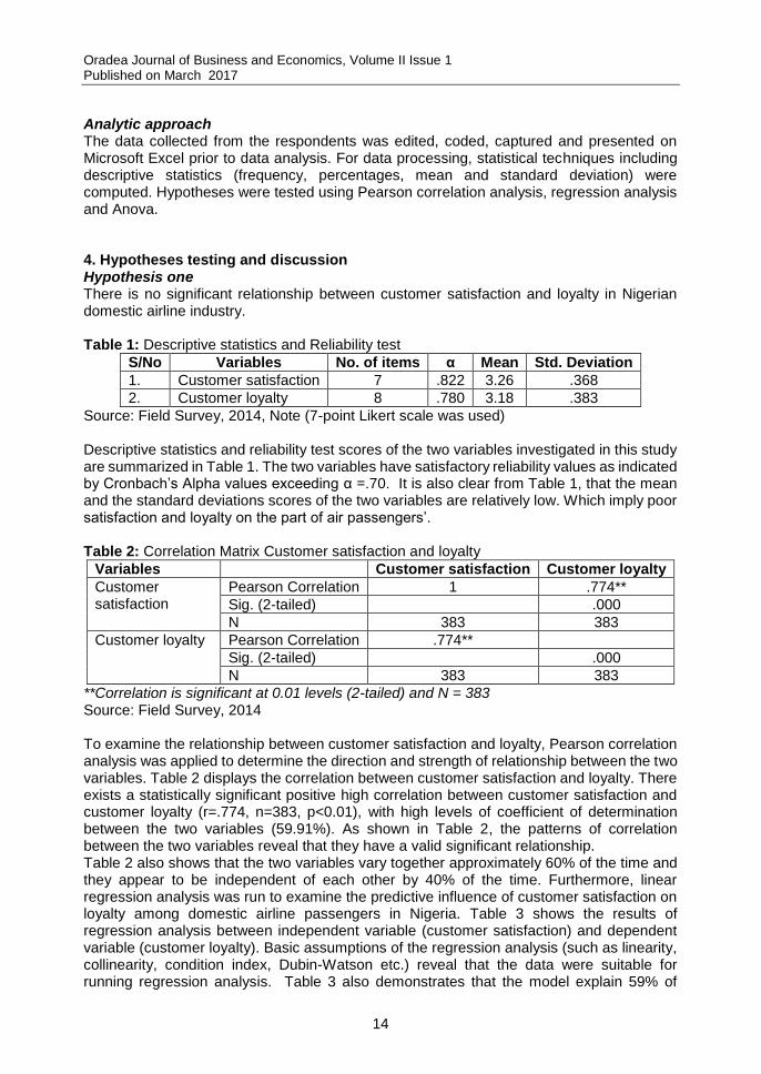
Analytic approach The data collected from the respondents was edited, coded, captured and presented on Microsoft Excel prior to data analysis. For data processing, statistical techniques including descriptive statistics (frequency, percentages, mean and standard deviation) were computed. Hypotheses were tested using Pearson correlation analysis, regression analysis and Anova. 4. Hypotheses testing and discussion Hypothesis one There is no significant relationship between customer satisfaction and loyalty in Nigerian domestic airline industry. Table 1: Descriptive statistics and Reliability test
S/No Variables No. of items α Mean Std. Deviation
1. Customer satisfaction 7 .822 3.26 .368
2. Customer loyalty 8 .780 3.18 .383
Source: Field Survey, 2014, Note (7-point Likert scale was used) Descriptive statistics and reliability test scores of the two variables investigated in this study are summarized in Table 1. The two variables have satisfactory reliability values as indicated by Cronbach’s Alpha values exceeding α =.70. It is also clear from Table 1, that the mean and the standard deviations scores of the two variables are relatively low. Which imply poor satisfaction and loyalty on the part of air passengers’. Table 2: Correlation Matrix Customer satisfaction and loyalty
Variables Customer satisfaction Customer loyalty
Customer satisfaction
Pearson Correlation 1 .774**
Sig. (2-tailed) .000
N 383 383
Customer loyalty Pearson Correlation .774**
Sig. (2-tailed) .000
N 383 383
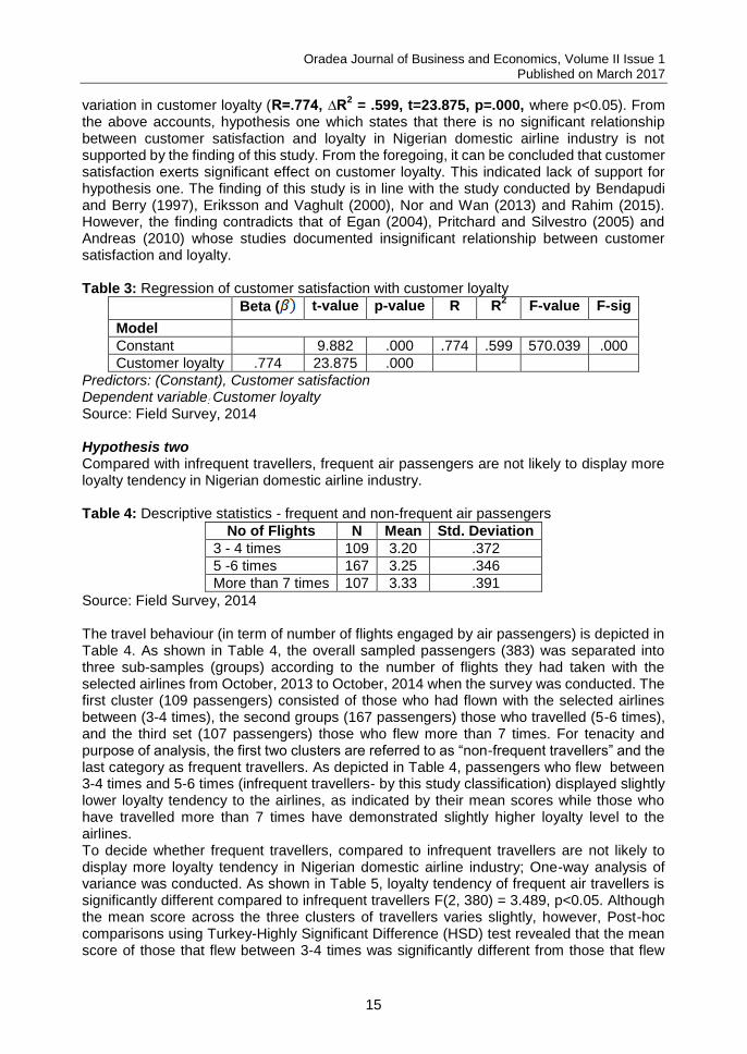
**Correlation is significant at 0.01 levels (2-tailed) and N = 383 Source: Field Survey, 2014 To examine the relationship between customer satisfaction and loyalty, Pearson correlation analysis was applied to determine the direction and strength of relationship between the two variables. Table 2 displays the correlation between customer satisfaction and loyalty. There exists a statistically significant positive high correlation between customer satisfaction and customer loyalty (r=.774, n=383, p<0.01), with high levels of coefficient of determination between the two variables (59.91%). As shown in Table 2, the patterns of correlation between the two variables reveal that they have a valid significant relationship. Table 2 also shows that the two variables vary together approximately 60% of the time and they appear to be independent of each other by 40% of the time. Furthermore, linear regression analysis was run to examine the predictive influence of customer satisfaction on loyalty among domestic airline passengers in Nigeria. Table 3 shows the results of regression analysis between independent variable (customer satisfaction) and dependent variable (customer loyalty). Basic assumptions of the regression analysis (such as linearity, collinearity, condition index, Dubin-Watson etc.) reveal that the data were suitable for running regression analysis. Table 3 also demonstrates that the model explain 59% of
Oradea Journal of Business and Economics, Volume II Issue 1 Published on March 2017
15
variation in customer loyalty (R=.774, ∆R2 = .599, t=23.875, p=.000, where p<0.05). From
the above accounts, hypothesis one which states that there is no significant relationship between customer satisfaction and loyalty in Nigerian domestic airline industry is not supported by the finding of this study. From the foregoing, it can be concluded that customer satisfaction exerts significant effect on customer loyalty. This indicated lack of support for hypothesis one. The finding of this study is in line with the study conducted by Bendapudi and Berry (1997), Eriksson and Vaghult (2000), Nor and Wan (2013) and Rahim (2015). However, the finding contradicts that of Egan (2004), Pritchard and Silvestro (2005) and Andreas (2010) whose studies documented insignificant relationship between customer satisfaction and loyalty. Table 3: Regression of customer satisfaction with customer loyalty
Beta ( t-value p-value R R2 F-value F-sig
Model
Constant 9.882 .000 .774 .599 570.039 .000
Customer loyalty .774 23.875 .000
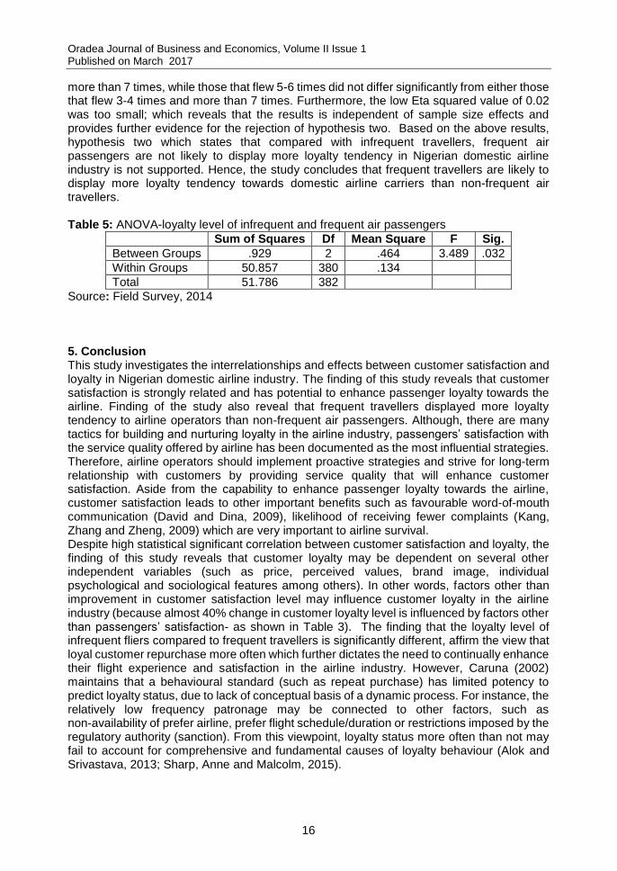
Predictors: (Constant), Customer satisfaction Dependent variable: Customer loyalty Source: Field Survey, 2014 Hypothesis two Compared with infrequent travellers, frequent air passengers are not likely to display more loyalty tendency in Nigerian domestic airline industry. Table 4: Descriptive statistics - frequent and non-frequent air passengers
No of Flights N Mean Std. Deviation
3 - 4 times 109 3.20 .372
5 -6 times 167 3.25 .346
More than 7 times 107 3.33 .391
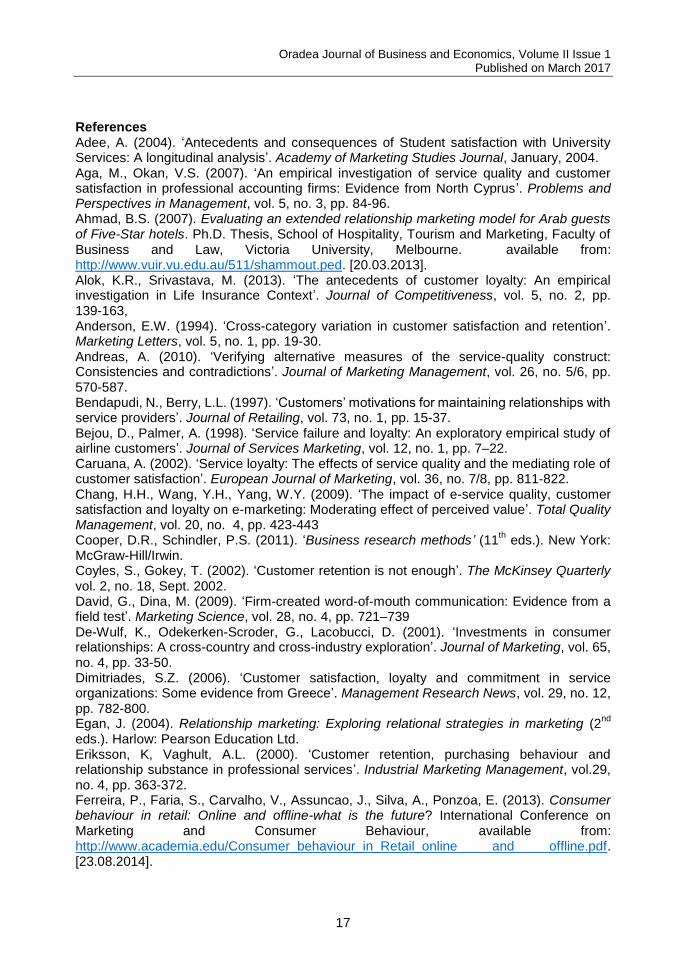
Source: Field Survey, 2014 The travel behaviour (in term of number of flights engaged by air passengers) is depicted in Table 4. As shown in Table 4, the overall sampled passengers (383) was separated into three sub-samples (groups) according to the number of flights they had taken with the selected airlines from October, 2013 to October, 2014 when the survey was conducted. The first cluster (109 passengers) consisted of those who had flown with the selected airlines between (3-4 times), the second groups (167 passengers) those who travelled (5-6 times), and the third set (107 passengers) those who flew more than 7 times. For tenacity and purpose of analysis, the first two clusters are referred to as “non-frequent travellers” and the last category as frequent travellers. As depicted in Table 4, passengers who flew between 3-4 times and 5-6 times (infrequent travellers- by this study classification) displayed slightly lower loyalty tendency to the airlines, as indicated by their mean scores while those who have travelled more than 7 times have demonstrated slightly higher loyalty level to the airlines. To decide whether frequent travellers, compared to infrequent travellers are not likely to display more loyalty tendency in Nigerian domestic airline industry; One-way analysis of variance was conducted. As shown in Table 5, loyalty tendency of frequent air travellers is significantly different compared to infrequent travellers F(2, 380) = 3.489, p<0.05. Although the mean score across the three clusters of travellers varies slightly, however, Post-hoc comparisons using Turkey-Highly Significant Difference (HSD) test revealed that the mean score of those that flew between 3-4 times was significantly different from those that flew
Oradea Journal of Business and Economics, Volume II Issue 1 Published on March 2017
16
more than 7 times, while those that flew 5-6 times did not differ significantly from either those that flew 3-4 times and more than 7 times. Furthermore, the low Eta squared value of 0.02 was too small; which reveals that the results is independent of sample size effects and provides further evidence for the rejection of hypothesis two. Based on the above results, hypothesis two which states that compared with infrequent travellers, frequent air passengers are not likely to display more loyalty tendency in Nigerian domestic airline industry is not supported. Hence, the study concludes that frequent travellers are likely to display more loyalty tendency towards domestic airline carriers than non-frequent air travellers. Table 5: ANOVA-loyalty level of infrequent and frequent air passengers
Sum of Squares Df Mean Square F Sig.
Between Groups .929 2 .464 3.489 .032
Within Groups 50.857 380 .134
Total 51.786 382
Source: Field Survey, 2014 5. Conclusion This study investigates the interrelationships and effects between customer satisfaction and loyalty in Nigerian domestic airline industry. The finding of this study reveals that customer satisfaction is strongly related and has potential to enhance passenger loyalty towards the airline. Finding of the study also reveal that frequent travellers displayed more loyalty tendency to airline operators than non-frequent air passengers. Although, there are many tactics for building and nurturing loyalty in the airline industry, passengers’ satisfaction with the service quality offered by airline has been documented as the most influential strategies. Therefore, airline operators should implement proactive strategies and strive for long-term relationship with customers by providing service quality that will enhance customer satisfaction. Aside from the capability to enhance passenger loyalty towards the airline, customer satisfaction leads to other important benefits such as favourable word-of-mouth communication (David and Dina, 2009), likelihood of receiving fewer complaints (Kang, Zhang and Zheng, 2009) which are very important to airline survival. Despite high statistical significant correlation between customer satisfaction and loyalty, the finding of this study reveals that customer loyalty may be dependent on several other independent variables (such as price, perceived values, brand image, individual psychological and sociological features among others). In other words, factors other than improvement in customer satisfaction level may influence customer loyalty in the airline industry (because almost 40% change in customer loyalty level is influenced by factors other than passengers’ satisfaction- as shown in Table 3). The finding that the loyalty level of infrequent fliers compared to frequent travellers is significantly different, affirm the view that loyal customer repurchase more often which further dictates the need to continually enhance their flight experience and satisfaction in the airline industry. However, Caruna (2002) maintains that a behavioural standard (such as repeat purchase) has limited potency to predict loyalty status, due to lack of conceptual basis of a dynamic process. For instance, the relatively low frequency patronage may be connected to other factors, such as non-availability of prefer airline, prefer flight schedule/duration or restrictions imposed by the regulatory authority (sanction). From this viewpoint, loyalty status more often than not may fail to account for comprehensive and fundamental causes of loyalty behaviour (Alok and Srivastava, 2013; Sharp, Anne and Malcolm, 2015).
Oradea Journal of Business and Economics, Volume II Issue 1 Published on March 2017
17
References Adee, A. (2004). ‘Antecedents and consequences of Student satisfaction with University Services: A longitudinal analysis’. Academy of Marketing Studies Journal, January, 2004. Aga, M., Okan, V.S. (2007). ‘An empirical investigation of service quality and customer satisfaction in professional accounting firms: Evidence from North Cyprus’. Problems and Perspectives in Management, vol. 5, no. 3, pp. 84-96. Ahmad, B.S. (2007). Evaluating an extended relationship marketing model for Arab guests of Five-Star hotels. Ph.D. Thesis, School of Hospitality, Tourism and Marketing, Faculty of Business and Law, Victoria University, Melbourne. available from: http://www.vuir.vu.edu.au/511/shammout.ped. [20.03.2013]. Alok, K.R., Srivastava, M. (2013). ‘The antecedents of customer loyalty: An empirical investigation in Life Insurance Context’. Journal of Competitiveness, vol. 5, no. 2, pp. 139-163, Anderson, E.W. (1994). ‘Cross-category variation in customer satisfaction and retention’. Marketing Letters, vol. 5, no. 1, pp. 19-30. Andreas, A. (2010). ‘Verifying alternative measures of the service-quality construct: Consistencies and contradictions’. Journal of Marketing Management, vol. 26, no. 5/6, pp. 570-587. Bendapudi, N., Berry, L.L. (1997). ‘Customers’ motivations for maintaining relationships with service providers’. Journal of Retailing, vol. 73, no. 1, pp. 15-37. Bejou, D., Palmer, A. (1998). ‘Service failure and loyalty: An exploratory empirical study of airline customers’. Journal of Services Marketing, vol. 12, no. 1, pp. 7–22. Caruana, A. (2002). ‘Service loyalty: The effects of service quality and the mediating role of customer satisfaction’. European Journal of Marketing, vol. 36, no. 7/8, pp. 811-822. Chang, H.H., Wang, Y.H., Yang, W.Y. (2009). ‘The impact of e-service quality, customer satisfaction and loyalty on e-marketing: Moderating effect of perceived value’. Total Quality Management, vol. 20, no. 4, pp. 423-443 Cooper, D.R., Schindler, P.S. (2011). ‘Business research methods’ (11
th eds.). New York:
McGraw-Hill/Irwin. Coyles, S., Gokey, T. (2002). ‘Customer retention is not enough’. The McKinsey Quarterly vol. 2, no. 18, Sept. 2002. David, G., Dina, M. (2009). ‘Firm-created word-of-mouth communication: Evidence from a field test’. Marketing Science, vol. 28, no. 4, pp. 721–739 De-Wulf, K., Odekerken-Scroder, G., Lacobucci, D. (2001). ‘Investments in consumer relationships: A cross-country and cross-industry exploration’. Journal of Marketing, vol. 65, no. 4, pp. 33-50. Dimitriades, S.Z. (2006). ‘Customer satisfaction, loyalty and commitment in service organizations: Some evidence from Greece’. Management Research News, vol. 29, no. 12, pp. 782-800. Egan, J. (2004). Relationship marketing: Exploring relational strategies in marketing (2
nd
eds.). Harlow: Pearson Education Ltd. Eriksson, K, Vaghult, A.L. (2000). ‘Customer retention, purchasing behaviour and relationship substance in professional services’. Industrial Marketing Management, vol.29, no. 4, pp. 363-372. Ferreira, P., Faria, S., Carvalho, V., Assuncao, J., Silva, A., Ponzoa, E. (2013). Consumer behaviour in retail: Online and offline-what is the future? International Conference on Marketing and Consumer Behaviour, available from: http://www.academia.edu/Consumer_behaviour_in_Retail_online and offline.pdf. [23.08.2014].
Oradea Journal of Business and Economics, Volume II Issue 1 Published on March 2017
18
Fraenkel, J.R., Wallen, N.E. (2000). How to design and evaluate research in education (4th ed.). New York: McGraw-Hill. Garbarino, E., Johnson, M.S. (1999). ‘The different roles of satisfaction, trust, and commitment in customer relationships’. Journal of Marketing, vol. 63 (April), pp. 70-87. Giese, J.L., Cote, J.A. (2002). ‘Defining consumer satisfaction’. Academy of Marketing Science Review, vol. 2, no. 1, pp. 1-24. Gilbert, D., Wong, R.K. C (2003). ‘Passenger expectations and airline services: A Hong Kong based study’. Tourism Management, vol. 24, pp. 519-532. Girden, E.R. (2001). Evaluating research articles (2
nd eds.). London: Sage Publications.
Gronholdt, L., Martensen, A., Kristensen, K. (2000). ‘The relationship between customer satisfaction and loyalty: Cross-industry differences’. Total Quality Management, vol. 11, no. 4-6, pp. 509-514 Helson, H. (1964). Adaptation-level theory. New York: Harper and Row. Hill, N., Alexander, J. (2000). Handbook of customer satisfaction and loyalty measurement (2
nd eds.). England: Gower Publishing Ltd.
Huang, Y.K., Feng, C.M. (2009). ‘Why customers stay: An analysis of service quality and switching cost on choice behaviour by Catastrophe Model’. International Journal of Services Operations and Informatics, vol. 4, no. 2, pp. 107-122. Iacobucci, D., Grayson, K.A., Ostrom, A.L. (1994). ‘The calculus of service quality and customer satisfaction: Theoretical and empirical differentiation and integration’. Advances in Services Marketing and Management, vol. 3, no. 1, pp. 67. Jones, T.O., Sasser, E. (1995). ‘Why satisfied customer defect’. Harvard Business Review, vol. 73, no. 6, pp. 88-99. Kang, J., Zhang, X., Zheng, Z. (2009). ‘The relationship of customer complaints, satisfaction and loyalty: Evidence from China’s mobile phone industry’. Journal of Marketing, vol. 8, no. 12, pp. 22-36. Kotler, P. (2001). Marketing management (10
th eds.). London: Prentice Hall International
Editions. McGill, A.L., Iacobucci, D. (1992). ‘The role of post-experience comparison standards in the evaluation of unfamiliar services’. Advances in Consumer Research. vol. 19, 570- 578. Miller, J.A. (1977). Studying satisfaction, modifying models, eliciting expectations, posing problems, and making meaningful measurements. In H.K. Hunt (Eds,). Conceptualization and measurement of consumer satisfaction and dissatisfaction. (pp. 72-91). Bloomington, IN: Indiana University School of Business. Mittal, V., Kamakura, W.A. (2001). ‘Satisfaction, repurchase intent, and repurchase behaviour: Investigating the moderating effect of customer characteristics’. Journal of Marketing Research, vol. 38, no. 1, pp. 131-142. Nadiri, H., Hussain, K., Ekiz, E.H., Erdogan, S. (2008). ‘An investigation on the factors influencing passengers’ loyalty in the North Cyprus national airline’. TQM Journal, vol. 20, no. 3, pp. 265–280. National Bureau of Statistics (2014). Nigerian Aviation Sector-Summary report of passenger traffic: 2010-2013 and Quarter One 2014. Available from: http://www.nigeriastat.gov.ng. [20.05.2014,] National Bureau of Statistics (2015). Nigerian Aviation Sector- Summary Report: Q2, 2015. available from: http://www.nigeriastat.gov.ng. [24.11.2016], Nor, K.A., Wan, N.M. (2013). ‘Perceptions of service quality and behavioural intentions: A mediation effect of patient satisfaction in the private health care in Malaysia’. International Journal of Marketing Studies, vol. 5, no. 4, pp. 15-29 Nordman, C. (2004). Understanding customer loyalty and disloyalty-The effect of loyalty supporting and re-pressing factors. Doctoral Thesis No. 125, Swedish School of economics and Business Administration, Helsinki, Finland, available from: http://www. Faculty.mu.edu.saidownload.pap?fid=50833.pdf. [20.05.2013].
Oradea Journal of Business and Economics, Volume II Issue 1 Published on March 2017
19
Oliver, R.L. (1977). ‘Effect of expectation and disconfirmation on post exposure product evaluations: An alternative interpretation’. Journal of Applied Psychology, vol. 62, no. 4, pp. 480-486. Oliver, R.L. (1980). ‘A cognitive model of the antecedents and consequences of satisfaction decisions’. Journal of Marketing Research, vol. 17 (November), pp. 460-490. Oliver, R.L. (1997). Satisfaction: A behavioural perspective on the consumer. New York: Irwin/McGraw-Hill. Oliver, R.L. (1999). ‘Whence customer loyalty?’ Journal of Marketing, 63, 33-44. Patterson, P.G. (1993). ‘Expectations and product performance as determinants of satisfaction for a high-involvement purchase’. Psychology Marketing, vol. 10, no. 5, pp. 449-466. Peyton, R.M., Pitss P.S., Kamery, R.H. (2003). Consumer satisfaction/dissatisfaction (CS/D): A review of the literature prior to the 1990s. Proceedings of the Academy of Organizational Culture, Communications and Conflicts, vol. 7, no. 2. Allied Academies International Conference. Las Vegas. pp. 41-46. Pizam, A., Ellis, T. (1999). ‘Customer satisfaction and its measurement in hospitality enterprises’. International Journal of Contemporary Hospitality Management, vol. 11, no. 7, pp. 326-339. Pritchard, M., Silvestro, R. (2005). ‘Applying the Service Profit Chain to analyse retail performance: The case of the Managerial Strait-jacket?’ International Journal of Service Industry Management, vol. 16, no. 4, pp. 337-356. Rahim, A.G., Ignatius, I.U., Adeoti, O.E. (2012). ‘Is customer satisfaction an indicator of customer loyalty?’ Australian Journal of Business and Management Research, vol. 2, no. 07, pp. 14-20. Rahim, A.G. (2015). Customer satisfaction and loyalty towards perceived service quality of domestic airlines in Nigeria. Unpublished Doctoral Thesis, University of Lagos, Lagos. Rahim, A.G. (2016a). ‘Perceptions of service quality: An empirical assessment of modified SERVQUAL Model among Domestic Airline Carriers in Nigeria’. Acta University Sapientiae, Economics and Business, vol. 4, pp. 5–31 Rahim, A.G. (2016b). ‘Perceived service quality and customer loyalty: The mediating effect of passenger satisfaction in the Nigerian Airline Industry’. International Journal of Management and Economics, vol. 52, October–December 2016, pp. 94–117 Ranaweera, C., Prabhu, J. (2003). ‘On the relative importance of customer satisfaction and trust as determinants of customer retention and positive word of mouth’. Journal of Targeting, Measurement and Analysis for Marketing, vol.12, no. 1, pp. 82-98. Reichheld, F. (2006). The ultimate question: Driving good profits and true growth (pp.1-28). Boston, Massachusetts: Harvard Business School Publishing Corporation. Reichheld, F.F., Sasser, Jr., W.E. (1990). ‘Zero defections: Quality comes to service’. Harvard Business Review, (September-October), pp. 105-111. Reichheld, F.F. (1996). ‘Learning from customer defections’. Harvard Business Review, (March/April), pp.56–69. Samaha, S.A., Palmatier, R.W., Dant, R.P. (2011). ‘Poisoning relationships: Perceived unfairness in channels of distribution’. Journal of Marketing, vol. 75, pp. 99-117. Sharp, B., Anne, S., Malcolm, W. (2015). Questioning the value of the “True” brand loyalty distinction. Marketing Science Centre, University of South Australia, available from: https://www.marketingscience.info/wp-content/uploads/staff/2015/08/6427.pdf. [12.11.2014].
Sheth, J.N., Mittal, B. (2004). Customer behavior: A managerial perspective (2nd
eds.). Mason, Ohio: Thomson/South-Western Shin, D., Elliott, K.M. (2001). ‘Measuring customers’ overall satisfaction: A multi-attributes assessment’. Services Marketing Quarterly, vol. 22, no. (1), pp. 3-19.
Oradea Journal of Business and Economics, Volume II Issue 1 Published on March 2017
20
Spreng, R.A., MacKenzie, S.B., Olshavsky, R.W. (1996). ‘A reexamination of the determinants of consumer satisfaction’. Journal of Marketing, vol. 60, no. 3, pp. 15- 32. Stanford Encyclopedia of Philosophy (2013). Loyalty, available from http://www. platostanford.edu/entries/loyalty/pdf. [24.12.2014]. StarmassInternational (2007). Your key to business success in China, available from: http://www.starmass.com/en/research_sampling_method.htm. [24.12.2014]. Struwig, F.W., Stead, G.B. (2001). Planning, designing and reporting research. Cape Town: Pearson Education South Africa. Swan, J.E., Oliver, R.L. (1989). ‘Post-purchase communications by consumers’. Journal of Retailing, vol. 65, no. 4, pp. 516–553. Taylor, T.B. (1998). ‘Better loyalty measurement leads to business solutions’. Marketing News, vol. 32, no. 22, pp. 41-42. Tim, K., Lerzan, A., Alexander, B., Luke, W. (2009). ‘Why a loyal customer isn’t always a profitable one’. The Wall Street Journal, (Monday June 22, 2009), CCL111(144). Timothy, L.K., Bruce,C., Lerzan, A., Tor, W.A., Jay, W. (2007). ‘The value of different customer satisfaction and loyalty metrics in predicting customer retention, recommendation and share-of-wallet’. Managing Service Quality, vol. 17, no. 4, pp. 361-384. Too, H.Y., Souchon, A.L., Thirkell, P.C. (2001). ‘Relationship marketing and customer loyalty in a retail setting: A dyadic exploration’. Journal of Marketing Management, vol. 17, no. 1, pp. 89-93. Uncles, M.D., Grahame, D.D, Kathy, H. (2003). ‘Customer loyalty and customer loyalty programs’. Journal of Consumer Marketing, vol. 20, no. 4, pp. 294–317. Vavra, T.G. (1997). Improving your measurement of customer satisfaction: A guide to creating, conducting, analyzing, and reporting customer satisfaction measurement programs. American Society for Quality. Whyte, R.D. (2011). Strategic windows: Australian European Union “open skies” agreement creates new entrant oppourtunity for long-haul low cost- airline model. Ph.D. Thesis, James Cook University, available from http://www.eprints.JCU.edu.au/23470. [24.06.2014]. Yang, Z., Jun, M., Peterson, R.T. (2004). ‘Measuring customer perceived online service quality’. International Journal of Operations and Production Management, vol. 24, no. 11, pp. 1149-1174. Yi, Y. (1990). A critical review of consumer satisfaction. In V. Zeithaml, (Eds.). Review of marketing (pp. 68-123). Chicago, IL: American Marekting Association. Yu-Kai, H. (2009). ‘The effect of airline service quality on passengers’ behavioural intentions using SERVQUAL scores: A Taiwan case study’. Journal of the Eastern Asia Society for Transportation Studies, vol. 8, pp. 1-17. Bio-note Rahim Ajao Ganiyu is lecturer in the Department of Business Administration, University of Lagos, Nigeria. Rahim moved into academic in 2016 with over 12 years industrial working experience in different industries/tasks. His employment experiences were primarily in marketing of industrial goods, oil and gas and property consulting. His research has been published in local and international journals. His areas of research interest include service quality, brand management, entrepreneurship, relationship marketing, project management, change management, consumer behavior, and development studies.
Oradea Journal of Business and Economics, Volume II Issue 1 Published on March 2017
21
CAN THERE BE A COMPETITOR TO TRADITIONAL ARABLE CROPS IN ROMANIA? Margit Csipkés Institute of Sectoral Economics and Methodology, Faculty of Economics and Business, University of Debrecen, Debrecen, Hungary [email protected] Abstract: Regarding land use, in the member states of the European Union it can be established that maize is the most productive traditional arable crop. The annual productive area of maize in 2015 was approximately 9.33 million hectares in the EU 28, which was 3% less than that of 2014. There was also a reduction in average production, which, according to member states’ figures decreased to 6.15 tonnes/ hectare. This reduction is due to the worsening natural conditions. Consequently, the year’s production was about 57 million tonnes at the end of 2015. This represented a reduction of 25% compared to 2014. The second largest production crop in the EU 28 is wheat, although here, too, a reduction can be observed when the data for the last 5 years is examined. This reduction in crop production prompts arable farmers to engage in the production of other crops in those areas where there is a continual reduction in crop production. In my study I will introduce the profitability and risks associated with those plants suited for energy extraction, which can be competitive with the traditional arable plant cultivation. Keywords: traditional arable crop, risk, energy, energy plants. JEL classification: O13, P18, Q42. 1. Romanian agriculture in 2015
On the basis of data from the National Institute of Statistics, the extent of agricultural territory decreased, compared to the previous year. On the basis of data for the last 10 years (NISA, 2012, OECD-FAO, 2010), this reduction is equivalent to about 1 million hectares. The official data records that agricultural areas (arable, pasture, feed crops) hardly reached 13 million hectares at the end of 2014. This means that Romania accounts for about 7 per cent of the Union’s agricultural territory. In first place is France with 28 per cent (~27.8 million hectares), followed by Spain with 13.60 per cent (23.75 million hectares), Great Britain with 9.7 per cent (16.88 million hectares), Germany with 9.6 per cent (16.7 million hectares) and Poland with 8.3 per cent (14.4 million hectares) (NISA, 2016). In Romania the average farm size is 3.6 hectares, which is four times smaller than the Union average (14.2 hectares). The greatest farm size in the EU 28 member states in 2015 is found in the Czech Republic, with 152.4 hectares, followed by Great Britain (90.4 hectares), Italy (79 hectares), Germany (55.8 hectares) and France (54 hectares). Naturally, the average does not give sufficient information about the size of the owning entities, since owners without a legal entity (e.g. farms maintained by sole proprietors) had farms which averaged 2 hectares, whereas farms with legal entity owners were about 200 hectares in size, according to figures for 2015. Despite the small size of farms compared to the Union average, about one third of all farms operating in the EU are found in Romania (32%). The division of agricultural land is 63 per cent arable, 33.7 per cent pasture and feed crops, 2.3 per cent fruit and vines, and 1.2 per cent family gardens.
Oradea Journal of Business and Economics, Volume II Issue 1 Published on March 2017
22
In plant production – according to the size of the area devoted to different crops – Romania is in the leading position for maize and sunflowers, since almost a quarter of the area devoted to these crops can be found in Romania. In the case of wheat, Romania is in fifth place, behind France, Germany, Poland and Spain. 2. The economic importance of energy crops
From the brief introduction to Romanian agriculture it can be seen that at the present time about 13 million hectares of land are given over to arable crops, while at the same time there are several hundred thousand hectares where even with the current support system it is difficult to ensure a profitable production from traditional arable crops. However, on these low productivity soils woody and herbaceous energy plants can be grown productively. In fields with high water tables these are primarily types of willow tree, while in areas with less water, they include the poplar, the acacia, Miscanthus (Chinese reed); and in clearly dry areas, energy grass. A more recent possibility is the Italian reed (Arundo D.) and giant Silphium perfoliatum. In addition to herbaceous energy plants, there is a possibility to grow energy seedlings, a method which does not require any change in the way the arable land is farmed, which also means that the subsidy for arable crops will be received by the farmer. The crop production cycle of the energy plants is, however, longer than that of arable crops. Through long term supplier contracts energy crops can represent a reliable and safe source of income, which, given the continually changing market conditions, the extremes of climate and the expected reduction in the European Union agricultural support, is something which is increasingly important for farmers. 3. Brief introduction to energy plants
One of the advantages of energy plants is that there is no (or hardly any) need for basic technical-technological changes in the cultivation method, and the biomass produce can be harvested annually - in some cases more frequently -, and because of the plants’ life cycle the number of harvests is high and they cannot be delayed. Herbaceous plants (the monocot species among them) make up the significant share of agricultural crops (the main ones include cereals, such as wheat, barley, oats and rye; and to a lesser extent sugar beet and cane sugar etc.). The seeds, roots and sometimes stalks of these plants are high sources of starch, and through various processes can thus be sources of bio-fuels and energy. The other herbaceous group are the perennial herbaceous plants, which are rapidly growing grass and reed species (e.g. the Italian reed – Arundo Donax), which can serve as both a source of high energy feed and basic energy material. Outside these two groups there is, for example, the energy reed (Miscanthus) group, which requires less water and so can be a good crop for agricultural areas with lower water supplies. 3.1. The biomass potential of energy plants
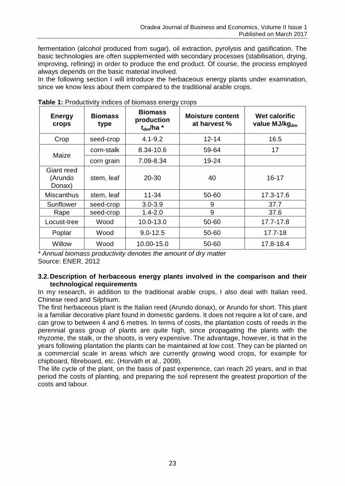
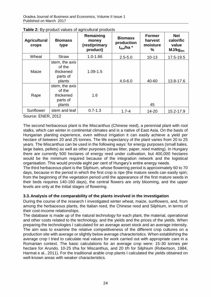
Agriculture is one of the sectors with the greatest biomass potential, since energy plants - and the bi-products of agricultural production - can be introduced into energy production. The biomass potential of individual energy plants can be seen in Table 1. As can be seen, in Romania, too, maize is the leading traditional arable crop, and so the energy potential of maize bi-products must also be investigated, since bi-products and waste material also have a significant energy potential, which can contribute to energy management (Table 2). The energy sources listed in Tables 1 and 2 can be processed by the help of various basic technologies: direct burning (electricity/heat production), anaerobic decomposition,
Oradea Journal of Business and Economics, Volume II Issue 1 Published on March 2017
23
fermentation (alcohol produced from sugar), oil extraction, pyrolysis and gasification. The basic technologies are often supplemented with secondary processes (stabilisation, drying, improving, refining) in order to produce the end product. Of course, the process employed always depends on the basic material involved. In the following section I will introduce the herbaceous energy plants under examination, since we know less about them compared to the traditional arable crops. Table 1: Productivity indices of biomass energy crops
Energy crops
Biomass type
Biomass production
tdm/ha *
Moisture content at harvest %
Wet calorific value MJ/kgdm
Crop seed-crop 4.1-9.2 12-14 16.5
Maize corn-stalk 8.34-10.6 59-64 17
corn grain 7.09-8.34 19-24
Giant reed (Arundo Donax)
stem, leaf 20-30 40 16-17
Miscanthus stem, leaf 11-34 50-60 17.3-17.6
Sunflower seed-crop 3.0-3.9 9 37.7
Rape seed-crop 1.4-2.0 9 37.6
Locust-tree Wood 10.0-13.0 50-60 17.7-17.8
Poplar Wood 9.0-12.5 50-60 17.7-18
Willow Wood 10.00-15.0 50-60 17.8-18.4
* Annual biomass productivity denotes the amount of dry matter Source: ENER, 2012 3.2. Description of herbaceous energy plants involved in the comparison and their
technological requirements In my research, in addition to the traditional arable crops, I also deal with Italian reed, Chinese reed and Silphium. The first herbaceous plant is the Italian reed (Arundo donax), or Arundo for short. This plant is a familiar decorative plant found in domestic gardens. It does not require a lot of care, and can grow to between 4 and 6 metres. In terms of costs, the plantation costs of reeds in the perennial grass group of plants are quite high, since propagating the plants with the rhyzome, the stalk, or the shoots, is very expensive. The advantage, however, is that in the years following plantation the plants can be maintained at low cost. They can be planted on a commercial scale in areas which are currently growing wood crops, for example for chipboard, fibreboard, etc. (Horváth et al., 2009). The life cycle of the plant, on the basis of past experience, can reach 20 years, and in that period the costs of planting, and preparing the soil represent the greatest proportion of the costs and labour.
Oradea Journal of Business and Economics, Volume II Issue 1 Published on March 2017
24
Table 2: By-product values of agricultural products
Agricultural crops
Biomass type
Remaining money
(rest/primary product)
Biomass production
tdm/ha *
Former harvest
moisture %
Net calorific
value MJ/kgdm
Wheat Straw 1.0-1.66 2.5-5.0 10-13 17.5-19.5
Maize
stem, the axis of the
thickened parts of plants
1.09-1.5
4.0-6.0 40-60 13.8-17.6
Rape
stem, the axis of the
thickened parts of plants
1.6
45
Sunflower stem and leaf 0.7-1.3 1.7-4 14-20 15.2-17.9
Source: ENER, 2012 The second herbaceous plant is the Miscanthus (Chinese reed), a perennial plant with root stalks, which can winter in continental climates and is a native of East Asia. On the basis of Hungarian planting experience, even without irrigation it can easily achieve a yield per hectare of between 20 and 25 tonnes. The life expectancy of the plant varies from 20 to 25 years. The Miscanthus can be used in the following ways: for energy purposes (small bales, large bales, pellets) as well as other purposes (straw litter, paper, reed matting). In Hungary there are currently 500 hectares of energy reed under cultivation, but 400,000 hectares would be the minimum required because of the integration network and the logistical organisation. This would provide eight per cent of Hungary’s entire energy needs. The third herbaceous plant is the Silphium, whose flowering period is approximately 60 to 70 days, because in the period in which the first crop is ripe (the mature seeds can easily spin; from the beginning of the vegetation period until the appearance of the first mature seeds in their beds requires 140-160 days), the central flowers are only blooming, and the upper levels are only at the initial stages of flowering. 3.3. Analysis of the comparability of the plants involved in the investigation
During the course of the research I investigated winter wheat, maize, sunflowers, and, from among the herbaceous plants, the Italian reed, the Chinese reed and Silphium, in terms of their cost-income relationships. The database is made up of the natural technology for each plant, the material, operational and other costs related to the technology, and the yields and the prices of the yields. When preparing the technologies I calculated for an average asset stock and an average intensity. The aim was to examine the relative competitiveness of the different crop cultures on a production site with average or slightly below average characteristics. When establishing the average crop I tried to calculate real values for work carried out with appropriate care in a Romanian context. The basic calculations for an average crop were: 15-30 tonnes per hectare for Arundo, 10-25 t/ha for Miscanthus, and 20 t/h for Silphium (Robertson, 1984, Harmat e al., 2011). For the traditional arable crop plants I calculated the yields obtained on well-known areas with weaker characteristics.
Oradea Journal of Business and Economics, Volume II Issue 1 Published on March 2017
25
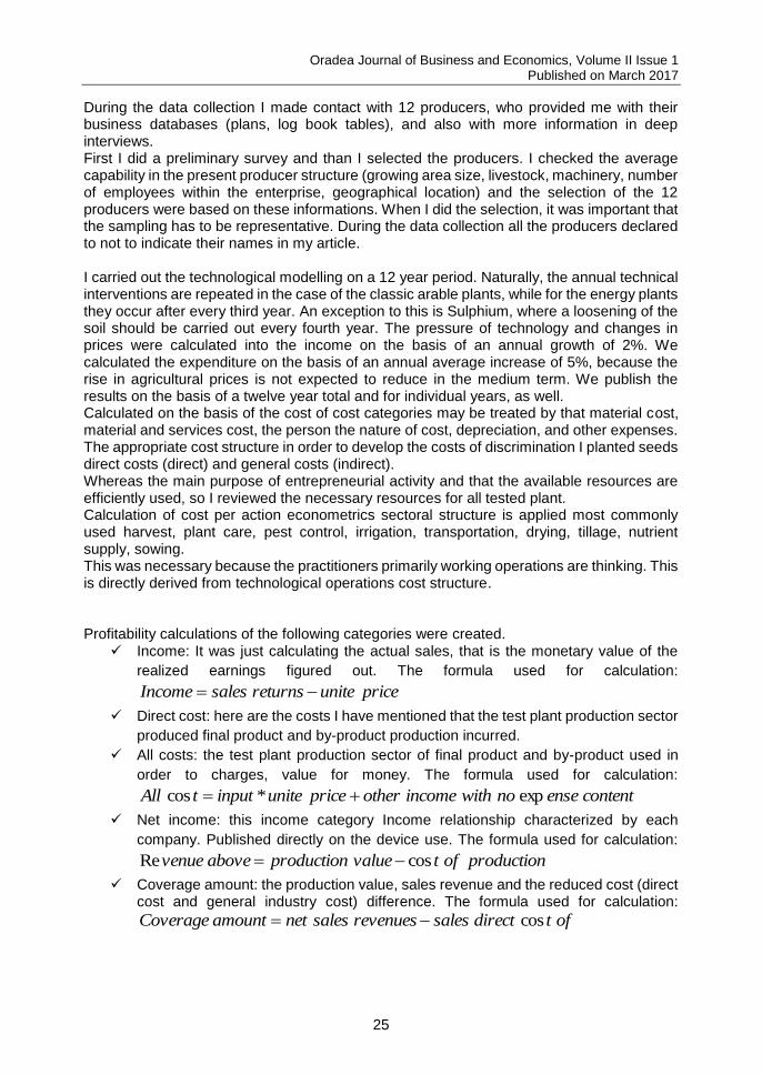
During the data collection I made contact with 12 producers, who provided me with their business databases (plans, log book tables), and also with more information in deep interviews. First I did a preliminary survey and than I selected the producers. I checked the average capability in the present producer structure (growing area size, livestock, machinery, number of employees within the enterprise, geographical location) and the selection of the 12 producers were based on these informations. When I did the selection, it was important that the sampling has to be representative. During the data collection all the producers declared to not to indicate their names in my article. I carried out the technological modelling on a 12 year period. Naturally, the annual technical interventions are repeated in the case of the classic arable plants, while for the energy plants they occur after every third year. An exception to this is Sulphium, where a loosening of the soil should be carried out every fourth year. The pressure of technology and changes in prices were calculated into the income on the basis of an annual growth of 2%. We calculated the expenditure on the basis of an annual average increase of 5%, because the rise in agricultural prices is not expected to reduce in the medium term. We publish the results on the basis of a twelve year total and for individual years, as well. Calculated on the basis of the cost of cost categories may be treated by that material cost, material and services cost, the person the nature of cost, depreciation, and other expenses. The appropriate cost structure in order to develop the costs of discrimination I planted seeds direct costs (direct) and general costs (indirect). Whereas the main purpose of entrepreneurial activity and that the available resources are efficiently used, so I reviewed the necessary resources for all tested plant. Calculation of cost per action econometrics sectoral structure is applied most commonly used harvest, plant care, pest control, irrigation, transportation, drying, tillage, nutrient supply, sowing. This was necessary because the practitioners primarily working operations are thinking. This is directly derived from technological operations cost structure. Profitability calculations of the following categories were created.
Income: It was just calculating the actual sales, that is the monetary value of the
realized earnings figured out. The formula used for calculation:
priceunitereturnssalesIncome
Direct cost: here are the costs I have mentioned that the test plant production sector
produced final product and by-product production incurred.
All costs: the test plant production sector of final product and by-product used in
order to charges, value for money. The formula used for calculation:
contentensenowithincomeotherpriceuniteinputtAll exp*cos
Net income: this income category Income relationship characterized by each
company. Published directly on the device use. The formula used for calculation:
productionoftvalueproductionabovevenue cosRe
Coverage amount: the production value, sales revenue and the reduced cost (direct cost and general industry cost) difference. The formula used for calculation:
oftdirectsalesrevenuessalesnetamountCoverage cos
Oradea Journal of Business and Economics, Volume II Issue 1 Published on March 2017
26
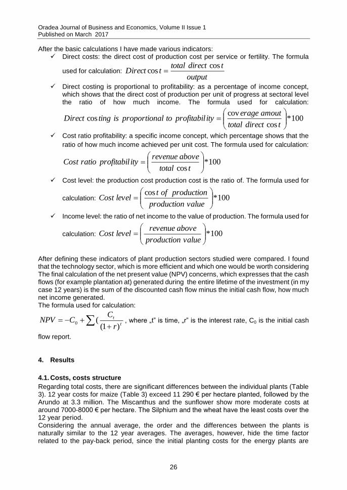
After the basic calculations I have made various indicators: Direct costs: the direct cost of production cost per service or fertility. The formula
used for calculation: output
tdirecttotaltDirect
coscos
Direct costing is proportional to profitability: as a percentage of income concept, which shows that the direct cost of production per unit of progress at sectoral level the ratio of how much income. The formula used for calculation:
100*cos
covcos
tdirecttotal
amouterageityprofitabiltoalproportionistingDirect
Cost ratio profitability: a specific income concept, which percentage shows that the
ratio of how much income achieved per unit cost. The formula used for calculation:
100*cos
ttotal
aboverevenueityprofitabilratioCost
Cost level: the production cost production cost is the ratio of. The formula used for
calculation: 100*cos
valueproduction
productionoftlevelCost
Income level: the ratio of net income to the value of production. The formula used for
calculation: 100*
valueproduction
aboverevenuelevelCost
After defining these indicators of plant production sectors studied were compared. I found that the technology sector, which is more efficient and which one would be worth considering The final calculation of the net present value (NPV) concerns, which expresses that the cash flows (for example plantation at) generated during the entire lifetime of the investment (in my case 12 years) is the sum of the discounted cash flow minus the initial cash flow, how much net income generated. The formula used for calculation:
t
t
r
CCNPV
)1((0
, where „t” is time, „r” is the interest rate, C0 is the initial cash
flow report. 4. Results
4.1. Costs, costs structure
Regarding total costs, there are significant differences between the individual plants (Table 3). 12 year costs for maize (Table 3) exceed 11 290 € per hectare planted, followed by the Arundo at 3.3 million. The Miscanthus and the sunflower show more moderate costs at around 7000-8000 € per hectare. The Silphium and the wheat have the least costs over the 12 year period. Considering the annual average, the order and the differences between the plants is naturally similar to the 12 year averages. The averages, however, hide the time factor related to the pay-back period, since the initial planting costs for the energy plants are
Oradea Journal of Business and Economics, Volume II Issue 1 Published on March 2017
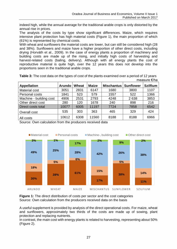
27
indeed high, while the annual average for the traditional arable crops is only distorted by the annual rise in prices. The analysis of the costs by type show significant differences. Maize, which requires intensive plant protection has high material costs (Figure 1), the main proportion of which (61%) is represented by chemical costs. With wheat and sunflowers the material costs are lower, but can still be considered high (28 and 38%). Sunflowers and maize have a higher proportion of other direct costs, including drying (Horváth et al., 2009). In the case of energy plants a proportion of machinery and building costs are made up of the rising, and initially high costs of harvesting and harvest-related costs (baling, delivery). Although with all energy plants the cost of reproductive material is quite high, over the 12 years this does not develop into the proportions seen in the traditional arable crops. Table 3: The cost data on the types of cost of the plants examined over a period of 12 years
measure €/ha
Appellation Arundo Wheat Maize Mischantus Sunflower Szilfium
Material cost 3051 2831 6147 1680 3800 1107
Personal costs 1841 523 579 1557 522 1366
Machine - building cost 4906 2531 2793 4248 2 638 3853
Other direct cost 280 120 1678 240 898 216
Direct costs total 10077 6005 11197 7724 7858 6542
Overall cost 535 303 363 465 329 424
All costs 10612 6308 11560 8188 8188 6966
Source: Own calculation from the producers received data
30%
28%61%
17%
38%
11%
18%
5%6%
15%
5%
14%
49%25%
28%42% 26%
38%
3% 1%17%
2%9%
2%
ARUNDO WHEAT MAIZE MISCHANTUS SUNFLOWER SZILF IUM
Material cost Personal costs Machine-, building cost Other direct cost
Figure 1: The direct distribution of costs per sector and the cost categories Source: Own calculation from the producers received data on the basis A useful supplement is provided by analysis of the direct operational costs. For maize, wheat and sunflowers, approximately two thirds of the costs are made up of sowing, plant protection and replacing nutrients. In contrast, the main cost with energy plants is related to harvesting, representing about 50% (Figure 2).
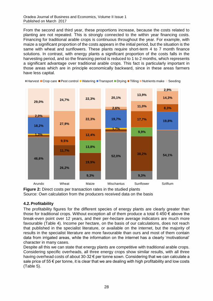
Oradea Journal of Business and Economics, Volume II Issue 1 Published on March 2017
28
From the second and third year, these proportions increase, because the costs related to planting are not repeated. This is strongly connected to the within year financing costs. Financing for traditional arable crops is continuous throughout the year. For example, with maize a significant proportion of the costs appears in the initial period, but the situation is the same with wheat and sunflowers. These plants require short-term 4 to 7 month finance solutions. In contrast, with energy plants a significant proportion of the costs falls in the harvesting period, and so the financing period is reduced to 1 to 2 months, which represents a significant advantage over traditional arable crops. This fact is particularly important in those areas which are in principle economically backward, since in these areas farmers have less capital.
46,6%
26,2%
9,3%
52,0%
9,3%
54,1%
11,7%
19,9%
38,2%
1,3%
1,7%18,2%
19,7%19,8%
13,8%
9,9%
9,5%
12,4%
17,7%
8,3%
2,0%
27,9%
22,3%
2,6%11,0%
14,3%
29,0%24,7% 22,3% 20,1%
13,9%
2,9%
Arundo Wheat Maize Mischantus Sunflower Szilfium
Harvest Crop care Pest control Watering Transport Drying Tilling Nutrients make Seeding
Figure 2: Direct costs per transaction rates in the studied plants Source: Own calculation from the producers received data on the basis 4.2. Profitability
The profitability figures for the different species of energy plants are clearly greater than those for traditional crops. Without exception all of them produce a total 6 450 € above the break-even point over 12 years, and their per-hectare average indicators are much more favourable (Table 4). Income per hectare, on the basis of our calculations, does not reach that published in the specialist literature, or available on the internet, but the majority of results in the specialist literature are more favourable than ours and most of them contain data from irrigated areas, while the information on the internet has a clearly ‘motivational’ character in many cases. Despite all this we can state that energy plants are competitive with traditional arable crops. Considering specific overheads, all three energy crops show similar results, with all three having overhead costs of about 30-32 € per tonne sown. Considering that we can calculate a sale price of 55 € per tonne, it is clear that we are dealing with high profitability and low costs (Table 5).
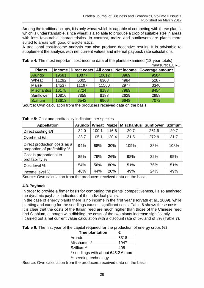
Oradea Journal of Business and Economics, Volume II Issue 1 Published on March 2017
29
Among the traditional crops, it is only wheat which is capable of competing with these plants, which is understandable, since wheat is also able to produce a crop of suitable size in areas with less favourable characteristics. In contrast, maize and sunflowers are plants more suited to areas with good characteristics. A traditional cost-income analysis can also produce deceptive results. It is advisable to supplement the analysis with net current values and internal payback rate calculations. Table 4: The most important cost-income data of the plants examined (12-year totals)
measure: EURO Plants Income Direct costs All costs Net income Coverage amount
Arundo 19581 10077 10612 8969 9504
Wheat 11292 6005 6308 4984 5287
Maize 14537 11197 11560 2977 3340
Mischantus 16178 7724 8188 7989 8454
Sunflower 10816 7858 8188 2629 2958
Szilfium 13613 6542 6966 6648 7072
Source: Own calculation from the producers received data on the basis Table 5: Cost and profitability indicators per species
Appellation Arundo Wheat Maize Mischantus Sunflower Szilfium
Direct costing €/t 32.0 100.1 116.6 29.7 261.9 29.7
Overhead €/t 33.7 105.1 120.4 31.5 272.9 31.7
Direct production costs as a proportion of profitability %
94% 88% 30% 109% 38% 108%
Cost is proportional to profitability %
85% 79% 26% 98% 32% 95%
Cost level % 54% 56% 80% 51% 76% 51%
Income level % 46% 44% 20% 49% 24% 49%
Source: Own calculation from the producers received data on the basis 4.3. Payback
In order to provide a firmer basis for comparing the plants’ competitiveness, I also analysed the dynamic payback indicators of the individual plants. In the case of energy plants there is no income in the first year (Horváth et al., 2009), while planting and caring for the seedlings causes significant costs. Table 6 shows these costs. It is clear that the costs of the Italian reed are much higher than those of the Chinese reed and Silphium, although with dibbling the costs of the two plants increase significantly. I carried out a net current value calculation with a discount rate of 5% and of 8% (Table 7). Table 6: The first year of the capital required for the production of energy crops (€)
Tree plantation €
Arundo 3318
Mischantus* 1947
Szilfium** 408
* seedlings with about 645.2 € more
** seeding technology
Source: Own calculation from the producers received data on the basis
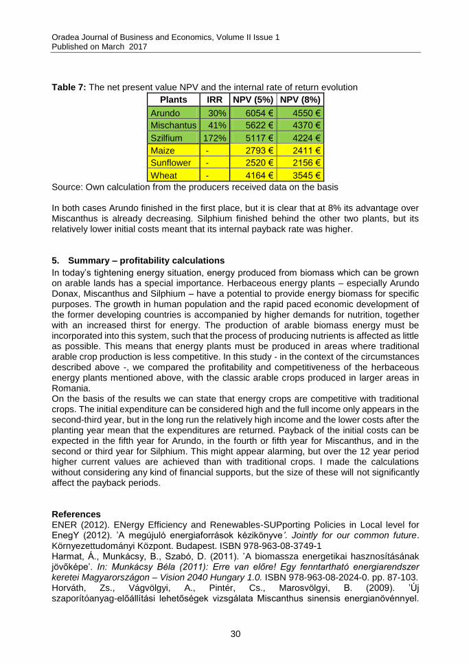
Oradea Journal of Business and Economics, Volume II Issue 1 Published on March 2017
30
Table 7: The net present value NPV and the internal rate of return evolution
Plants IRR NPV (5%) NPV (8%)
Arundo 30% 6054 € 4550 €
Mischantus 41% 5622 € 4370 €
Szilfium 172% 5117 € 4224 €
Maize - 2793 € 2411 €
Sunflower - 2520 € 2156 €
Wheat - 4164 € 3545 €
Source: Own calculation from the producers received data on the basis In both cases Arundo finished in the first place, but it is clear that at 8% its advantage over Miscanthus is already decreasing. Silphium finished behind the other two plants, but its relatively lower initial costs meant that its internal payback rate was higher. 5. Summary – profitability calculations
In today’s tightening energy situation, energy produced from biomass which can be grown on arable lands has a special importance. Herbaceous energy plants – especially Arundo Donax, Miscanthus and Silphium – have a potential to provide energy biomass for specific purposes. The growth in human population and the rapid paced economic development of the former developing countries is accompanied by higher demands for nutrition, together with an increased thirst for energy. The production of arable biomass energy must be incorporated into this system, such that the process of producing nutrients is affected as little as possible. This means that energy plants must be produced in areas where traditional arable crop production is less competitive. In this study - in the context of the circumstances described above -, we compared the profitability and competitiveness of the herbaceous energy plants mentioned above, with the classic arable crops produced in larger areas in Romania. On the basis of the results we can state that energy crops are competitive with traditional crops. The initial expenditure can be considered high and the full income only appears in the second-third year, but in the long run the relatively high income and the lower costs after the planting year mean that the expenditures are returned. Payback of the initial costs can be expected in the fifth year for Arundo, in the fourth or fifth year for Miscanthus, and in the second or third year for Silphium. This might appear alarming, but over the 12 year period higher current values are achieved than with traditional crops. I made the calculations without considering any kind of financial supports, but the size of these will not significantly affect the payback periods. References ENER (2012). ENergy Efficiency and Renewables-SUPporting Policies in Local level for EnegY (2012). ’A megújuló energiaforrások kézikönyve’. Jointly for our common future. Környezettudományi Központ. Budapest. ISBN 978-963-08-3749-1 Harmat, Á., Munkácsy, B., Szabó, D. (2011). ’A biomassza energetikai hasznosításának jövőképe’. In: Munkácsy Béla (2011): Erre van előre! Egy fenntartható energiarendszer keretei Magyarországon – Vision 2040 Hungary 1.0. ISBN 978-963-08-2024-0. pp. 87-103. Horváth, Zs., Vágvölgyi, A., Pintér, Cs., Marosvölgyi, B. (2009). ’Új szaporítóanyag-előállítási lehetőségek vizsgálata Miscanthus sinensis energianövénnyel.
Oradea Journal of Business and Economics, Volume II Issue 1 Published on March 2017
31
Nyíradony-Gúthpuszta Konferenciakiadvány. Alföldi Erdőkért Egyesület. Kutatói nap. Tudományos eredmények a gyakorlatban. pp. 89-93. INS, (2012). National Institute of Statistics. ’Agricultural holdings, number of persons, by gender, and number of worked days, by size classes of number of worked days, by legal status of agricultural holding’, available from http://www.insse.ro/cms/ro/content/ancheta-structural%C4%83-%C3%AEn-agricultur%C4%83-2013-date-pe-macroregiuni-regiuni-de-dezvoltare-%C5%9Fi-jude%C5%A3e [05.02.2017]. INS (2016). National Institute of Statistics. ’Ancheta Structurală în Agricultură 2016 Date pe Macroregiuni, regiuni de dezvoltare şi judeţe - Volumul II’, available from http://www.insse.ro/cms/ro/content/ancheta-structural%C4%83-%C3%AEn-agricultur%C4%83-2016-date-pe-macroregiuni-regiuni-de-dezvoltare-%C5%9Fi-jude%C5%A3e [17.01.2017]. OECD-FAO (2010). OECD-FAO (Food and Agriculture Organization of the United Nations) Agricultural Outlook 2015-2024. ’Overview of the OECD-FAO Agricultural Outlook 2015-2024.’ Paris. ISBN 978-92-64-23190-0 Robertson, A.W., Khail, M.A.K. (1984). ’Conifers for Biomass production’. Vol. I. Forest Energy Program, Canadian Forestry Service and I.E.A. In. W. Palz – J. Coombs – D.O. Hall: Energy from biomass 3rd E.C. Conference Elsevier applied science publishers. Brussels and Luxemburg. ISBN 0-85334-3969. pp. 303-315. Bio-note
Margit Csipkés, Ph.D. is a senior lecturer at University of Debrecen Faculty of Economics and Business, Institute of Sectoral Economics and Methodology. Her research topic is the traditional arable crops, energy crops and land use role. She earned PhD in economic analysis of individual power plants as well as their impact on land use. She is currently researching the energy management policies of Hungary and surrounding countries. In this respect, she typically uses statistical methods, R program, linear programming and economic analysis.
Oradea Journal of Business and Economics, Volume II Issue 1 Published on March 2017
32
USING WAVELETS IN ECONOMICS. AN APPLICATION ON THE ANALYSIS OF WAGE-PRICE RELATION
Vasile-Aurel Caus1, Daniel Badulescu
2, Mircea Cristian Gherman3
1Department of Mathematics, University of Oradea, Oradea, Romania
2Department of Economics, University of Oradea, Oradea, Romania
3Technical University of Cluj-Napoca, Romania
[email protected] [email protected] [email protected] Abstract: In the last decades, more and more approaches of economic issues have used mathematical tools, and among the most recent ones, spectral and wavelet methods are to be distinguished. If in the case of spectral analysis the approaches and results are sufficiently clear, while the use of wavelet decomposition, especially in the analysis of time series, is not fully valorized. The purpose of this paper is to emphasize how these methods are useful for time series analysis. After theoretical considerations on Fourier transforms versus wavelet transforms, we have presented the methodology we have used and the results obtained by using wavelets in the analysis of wage-price relation, based on some empirical data. The data we have used is concerning the Romanian economy - the inflation and the average nominal wage denominated in US dollars, between January 1991 and May 2016, highlighting that the relation between nominal salary and prices can be revealed more accurately by use of wavelets.
Key-words: wage-price spiral, wavelet transforms, Fourier transforms, spectral analysis. JEL classification: C02, C32, E31. 1. Introduction The last decades witnessed the development of mathematical tools dedicated to economic analysis. Starting with Nash’s pioneering work, there is an increased concern for searching economic applications of mathematical methods and tools. In the same time, the problem of evaluating and testing the utility of used mathematical methods has emerged. Analysis of economic phenomena is, by its nature, intended to identify components and their impact on the fulfillment of economic processes. Most often this operation is difficult and involves the use of mathematically complex tools, among which wavelet method is to be mention. The objective of this article is to emphasize the usefulness of these methods in time series analysis. The article is organized as follows. In the first part we present how Fourier and wavelet transforms are used in economics, and the differences between the two methods. In the second part we present the methodology used, in the third part we present the findings and results obtained by using wavelet analysis applied on wage-price relation, based on some empirical data, and finally we conclude.
Corresponding author
Oradea Journal of Business and Economics, Volume II Issue 1 Published on March 2017
33
2. Theoretical overview on wavelet transforms used in economics The wavelets theory has developed very rapidly in the last twenty years. There are various applications of wavelets, related to: signal analysis, astronomy, medicine (especially imagistic), geology, meteorology, physics, etc. We would have expect that dual time-frequency properties and the ability to work both on stationary and non-stationary series recommend wavelets as an effective mathematical tool in economics, especially in financial macroeconomics. However, there are few works dealing with the application of wavelets in economics. Therefore, we consider that any contribution highlighting the efficiency and consistency of the "wavelet analysis" in economics is useful in developing economic modeling techniques. Time series analysis is probably the most important chapter of econometrics (and not only). The main purpose (in economic terms) of this type of analysis is to identify a function or at least an argument to allow a forecast of the future values of the series in question. In other words, in most cases, it is about predicting the future based on past analysis. Economic phenomena represented by time series and subject of analysis are not always simple; on the contrary, they are often difficult to analyze. This is due, in most cases, to the difficulty of identifying and isolating the analyzed components of the phenomenon (trend, seasonality, etc.). Therefore, the analysis of the economic phenomena, time related, although efficient in many situations, is insufficient in other cases. Graphs, so common in economic presentations, are mostly in the time-amplitude area: on the horizontal axis time is represented, and on the vertical axis the values - measured, calculated or predicted – of the time-dependent variable. This representation, while very often useful, hides, in the case of complex phenomena, the most important features. This is the main reason for developing mathematical tools to transform these representations into more suggestive ones. The stated purpose of applying transforms on economic time series is to identify the main components of the phenomena, the frequency and the amplitude of them. Once identified and isolated these components, they can be easier analyzed and their behavior can be predicted with a higher degree of accuracy than in the case of the time-analysis of the original series. Since the original series can be reconstructed based on the components, the prediction arguments developed on the latter ones can be extended to the original series, considering, of course, the interdependence between them. A first transform used in many economic analyses is the Fourier transform (continuous, discrete, fast etc.). Basically, by applying this transformation, we pass from the time-domain into the frequency-domain. In other words, the horizontal axis shows frequencies, and the vertical axis shows amplitudes. A crucial observation is that, when using Fourier transform, the graph does not contain time. Specifically, Fourier transform can tell us which are the frequencies of the main components of the analyzed phenomenon, but it cannot provide information about the moments, in time, when these frequencies occur. Even if, as we mentioned, the original series can be reconstructed from Fourier transform, in other words we can pass anytime from one representation to another (from the time domain to frequency domain and vice versa) we cannot obtain simultaneously information on time, frequency, amplitude. For this reason Fourier transformation is used only for stationary series (series which do not change their frequency structure over time). There is a rich literature on Fourier analysis (or spectral analysis). The first important treaty is C.W.J. Granger’s "Spectral analysis of economic time series" (1964). Another master work is M.B. Priestley’s "Spectral analysis and time series" (1981), but also dedicated book chapters in Hamilton’s "Time Series Analysis" (1994) or Handbook of Econometrics, Volume II (Griliches and Intriligator, editors) (1984). Among the recent works, we mention Bloomfield’s "Fourier Analysis of Time Series" (2000) and Broersen’s "Automatic Autocorrelation and Spectral Analysis” (2006). Of course, there are hundreds of articles published in academic journals.
Oradea Journal of Business and Economics, Volume II Issue 1 Published on March 2017
34
Unfortunately, as we mentioned, the Fourier transform is inefficient for non-stationary series because it provides single information: the spectral composition or spectrum (which frequencies and amplitudes do the components of the analyzed series have), without being able to highlight the changes during time of the spectrum. As expected, the spectral analysis relies on the term “light spectrum”. Just as light, it can be split into several components with different frequency composing the spectrum and which are invisible to the eye unless a transformation is used (e.g. a prism in the beam path), so that a phenomenon represented by a time series may contain components undetectable in the absence of transformation. The Fourier transform default is related to the failure to provide information on the time location of the spectral structure. If an economic series needs a time-frequency representation it is necessary to use another transform. Before presenting this more powerful transformation, we have to remember that the use of Fourier transform with some restrictions generate variants (short time Fourier transform, windowed Fourier transform) that allow a time-frequency analysis. This can be done, for example, by using frequency filters which decompose the signal in frequency bands with given width. The 3D representation of this decomposition uses one time axis, one for frequencies and one for amplitude. This representation is most of the time unsatisfactory because doesn’t allow to modify the resolution (more information about this scale is found in the works mentioned in the bibliography, especially those relating to wavelets). This brings us, finally, to wavelets. Wavelets, as suggested by their names, are small waves. The most important feature is that they have local support, in other words, their value is different than zero on a finite and bounded interval, but in the rest they have the zero value. Why is this important? Let us return to Fourier transform. Although we haven’t presented the analytical expression of this transformation, we can imagine that changing a coefficient in the expression of Fourier transform attached to a function or to a discrete series produces changes spread through all the period (i.e. changes cannot be located in time). In other words, let’s suppose that we intervene on a point of a metal band swing. Our intervention will affect the band swings from one end to another. Thus, we cannot analyze the effect of spectral changes at some given moment as these changes are transmitted through the whole series. There is an essential difference between wavelet transform and Fourier transform. Because wavelets have non-zero values on sufficiently small intervals, when you change the coefficients in the series representation through wavelets, the effect diminishes quickly enough. Because, finally, everything comes down to this: the determination of the values or analytical expressions of some coefficients in order to obtain a better (or the best) approximation of the dynamics of an economic phenomenon. As we mentioned, there is yet another important distinction between Fourier transform and wavelet transform. The latter allows a multi-resolution analysis, while Fourier analysis does not allow changing the resolution. The resolution adaptation (or change) on the spectrum series is very important. It is obvious that, at a low resolution, the image can be seen entirely, but details are lost; while at high resolution we identify details, but the overall picture is lost. Therefore, the multi-resolution analysis uses high resolution for time and small for frequency in the case of high frequencies, respectively small resolutions for time and high resolutions for frequencies in the case of low frequencies. The reason for which we cannot use simultaneously high resolutions for both time and frequencies is derived from Heisenberg's uncertainty principle. This is the reason determining, when necessary, the use of transformations (as it is the wavelet transformation) allowing the adaptation of the resolution. If we consider economic time series, in most cases they contain a low frequency and longtime duration trend and seasonality or disturbance of (relatively) high frequency with a short event. The wavelet transformation consists mainly in the application of an operator on the regression function constructed on the base of previous observations.
Oradea Journal of Business and Economics, Volume II Issue 1 Published on March 2017
35
First, we note that this transformation uses two categories of wavelets: mother wavelets and father wavelets. The mother wavelets have the property that:
0)( dtt ,
and father wavelets have the property that:
1)( dtt .
Any function )(tf can be represented as a linear combination of mother and father
wavelets. If, for example, )(t and )(t are symmetrical mother and father wavelets (so
called symmlets), then they can be expressed as:
Zkjkttj
j
kj
, ),2(2)( 2,
and
Zkjkttj
j
kj
, ),2(2)( 2,
. Obviously, symmetrical wavelets are not the only wavelets that can be used in practical applications.
The )(tf function can therefore be represented as:
k k
kkkNkN
k k
kNkNkNkN tdtdtdtstf )(...)()()()( ,1,1,1,1,,,,
where dtttfs kNkN )()( ,, and },...,2,1{ ,)()( ,, Njdtttfd kjkj are the
transformation coefficients. In this representation j is the scale used, and k is the number of translations corresponding to each scale, while N is the maximum value of the scale used in the representation. The
functions )(, tkN and )(, tkN must fulfill the condition that they form an orthogonal basis.
If we denote
k
kNkNN tsS )(,,
and
k
kNkNN tdD )(,, , then multi-resolution
decomposition of the function )(tf is given by },...,,,{ 11 DDDS NNN .
The described representation corresponds to a discrete variable (the most common case encountered in economic data analysis) and the transformation is called transformation by discrete wavelets, unlike the continuous case (wavelets continuous transformation) using integral operators. The information on time series are obtained by the analysis of partial sums,
)(...)()()()( 11 tDtDtDtStS jNNNj ,
providing information on the dynamics (frequency and time) of the components that are most relevant for the series’ behavior. Once these components are identified, they can be "cleaned" and assembled in order to build an approximation of the original series.
Oradea Journal of Business and Economics, Volume II Issue 1 Published on March 2017
36
A graphical scheme that explains easy the algorithm of using the discrete transformation by wavelets and the use of the inverse transform (for the series’ reconstruction) can be found in Crowley (2007). 3. Methodology: thresholding with wavelets Economic time series and financial data contain information which is sometimes considered to be un-useful or unwanted. For better prediction accuracy, it is necessary to smooth the data or to filter out the noise (perturbation). This technique is often called de-noising and can be accomplished with wavelets transforms too, see Donoho and Johnstone (1995). A de-noising algorithm could be used in order to “clean” any signal (time series) that contains the unwanted noise (Karim, et al., 2011). Since the wavelet transform is a set of coefficients representing the time series in a wavelet domain, the techniques applied in this domain will affect also the series in the time domain. One reason of performing some processing on other domain is that the detail and approximations scales are very well defined and also very clearly represented in such kind of transformations. As a consequence, wavelet filtering acts as a smoothing operator. Not the same can be affirmed about Fourier basis. By shrinking Fourier coefficients, we can get bad results in terms of mean square error. Also, some visual artifacts can be observed in the filtered time series as stated in Donoho (1993). The filtering technique in wavelet domain is often called thresholding and it is based on the idea that the majority of wavelet coefficients correspond to details (Al Wadi, et al., 2011). When details are small, they might be omitted without substantially affecting the "general picture." Thus the idea of thresholding wavelet coefficients is a way of cleaning out "unimportant" details considered to be noise. Thresholding is a good technique in time series processing due to the fact that the parsimony of wavelet transformations ensures that the signal of interest can be well described by a relatively small number of wavelet coefficients. The process of thresholding wavelet coefficients can be divided into two steps. The first step is the choice of the threshold function T. There are two main rules of thresholding: soft thresholding or hard thresholding. Given a wavelet coefficient w and threshold value λ, the corresponding transformation for hard threshold value of the coefficient can be written as (Karim, et al., 2011):
)|(|),( wwIwThard ,
On the other hand, for the soft threshold the previous transformation becomes:
)|(|)|)(|(),( wIwwsignwTsoft , Where I is the usual indicator function.
In other words, “hard” means “keep or kill” while “soft” means “shrink or kill”, see Hardle et al. (1998) or Van Fleet (2008). The commonly adopted rule is to use soft thresholding. Although the hard thresholding is able to preserve the peak, it also produces more spurious oscillations and close discontinuities (Karim et al., 2011). The second step is the choice of a threshold. In the following sections we briefly present some considerations about methods of selecting a threshold. In financial applications (Ramsey, 2002), soft thresholding methods or some combined method between the two are often used. Depending on the application, other types of thresholding can be used, which have several approaches. Wang (1994) generalizes Nason's cross validation technique by removing more than half of the data each time. The motivation is to improve the robustness of the threshold selection procedure against the effect of a correlated noise (with long range dependence). Saito (1994) incorporates the hard thresholding into a minimum description length procedure. Vidakovic (1994) describes wavelet shrinkage via Bayes rules and Bayesian testing of hypothesis.
Oradea Journal of Business and Economics, Volume II Issue 1 Published on March 2017
37
In this study we have applied the modified thresholding algorithm based on the Donoho and Johnstone (1995) threshold method. This is based on some prerequisite assumptions. If z is
a random variable having its elements iz independent and normal identically distributed
(i.i.d. - )1,0(~ Nzi ), then it can be defined the following variable:
ninzA in ,1};log2{max .
The nA is defined in such a way that nAP nn ,0)( . In addition, if
}}log2{max)( ntztB in for every sample of the z dataset (i=1,n), then
2/2
))((t
n etBP .
That motivates the following threshold: ˆlog2 nU
, which is meant to be universal. In
this expression the variance of the analyzed data is considered to be ̂ .This threshold is one of
the first proposed and provides a fast and, in the same time, easy and automatic thresholding. The reason behind this is to remove all wavelet coefficients that are smaller than the expected maximum of an assumed i.i.d. noise sequence of given size (n). Hence, there are several
possibilities to estimate the variance ̂ from the above expression.
Almost all thresholding methods involve the wavelet coefficients of the finest scale which are considered to be strongly related to the noise since these scales represent the most detailed elements of the analyzed time series. The signal-to-noise ratio is smallest at high resolutions in wavelet decomposition for almost all signals. Some standard estimators are:
2/
1
2,1
2)(
12/
1ˆ
N
i in wwN
or a more robust
})2/,1,({6745.0/1ˆ ,12 NiwMAD in
Where n is the highest level of the wavelet transform. In some applications, especially if using the first estimator and the data sets are large , and when is overestimated like in the case when using the second estimator, the universal
thresholding can give under-fitted models. As a matter of fact one can use a simple algorithm in order to de-noise a financial time series. The step of this kind of algorithm can be resumed as following: 1) First, based on its properties, choose the basis wavelet function and the number of scale levels for signal decomposition 2) Apply a wavelet transform to the original signal (time series) and create the matrix transformation 3) Remove the small (detail/wavelets) coefficients by using a thresholding method 4) Perform other processing or adjustments to the wavelet coefficients, if needed 5) Reconstruct the original signal by applying the inverse wavelet transform to the processed transformation. After applying all these steps we obtain the reconstruct time series having some “new” properties based on which one can take different decisions in the economic field, including here the relation between inflation and nominal wages.
Oradea Journal of Business and Economics, Volume II Issue 1 Published on March 2017
38
4. An application on wage-price relation. Findings and results In this section we consider an application concerning the relation between salaries (wages) and inflation (prices). We will briefly present a short theoretical overview on the relation investigated, and then present our findings related to the applied method regarding filtering and thresholding the economic time series. During the last decades, finding a relation between wage growth and periodic inflation kept the attention of economists, hoping to understand the developments on the labor market which may be a good predictor of inflationary pressures. A clear argument for how labor costs tend to push up prices, i.e. the so-called wage-price spiral, is synthesized in Layard, Nickell and Jackman (1994). They stated that “when buoyant demand reduces unemployment (at least relative to recent experienced levels), inflationary pressure develops. Therefore, the companies start bidding against each other for labor, and workers feel more confident in pressing wage claims. If the inflationary pressure is too great, inflation starts spiraling upwards: higher wages lead to higher price rises, leading to still higher wage rises, and so on” (Layard et al., 1994). This is the wage-price spiral presented in the mentioned work. In respect to this, we can notice a re-evaluation of the cost push type models of inflation, the estimations and statistical analysis trying to see if the production cost channel is a credible mechanism for price increases. Another important approach is mentioned in Aristide (2007). Thus, if the aggregate demand is maintained constant, then the productivity, the competitive pressures and the profit rate of enterprises will increase the labor costs (also with fiscal taxes and raw materials) which will be reflected in increased economic prices (Badulescu and Caus, 2011). Tracking statistics data indicates, at least apparently, an "in tandem" movement of wages and prices, but this cannot convince the researchers to unanimously consider that wages growth leads to rising prices, i.e. inflation. In fact, the last decades show that there are two main approaches analyzing and interpreting statistical data in wage-inflation relation. On one hand, works such as Gordon (1988), Rissman (1995) quoted in Hess and Schweitzer (2000), Clark (1998), and, partially, Jonsson and Palmqvist (2004) state that there is no strong evidence of the relation between these two variables. On the other hand, we can mention the works of Ghali (1999) or Aaronson (2001) sustaining a significant relation between wage growth and inflation. In the same trend, some papers and works undertaken by the European Central Bank show that, on the short run, an inflationary process can result from increases in factors such as consumption, investment, widening budget deficits, energy costs or wages uncorrelated with productivity gains. Inflationary pressure may also occur if the "workers and unions would have doubts about future inflation, and therefore they would require a considerable increase of nominal wages to avoid a strong future inflation leading to significant decreases in real wages" (European Central Bank, 2011). As a conclusion to these approaches, we can say that increasing the unit labor cost may be an important element for a series of economic variables (such as the trade deficit), but it affects in lower measure the prices adjusted with productivity (Badulescu and Caus, 2010). We will try to identify whether there is or there is not a strong relation between wages and prices (inflation). The data we have used is concerning the Romanian economy and it has been provided by the Romanian Institute of Statistics. The two economic series, the inflation and the average nominal wage denominated in US dollars are considered on a monthly basis. The covered period is from January 1991 to May 2016.
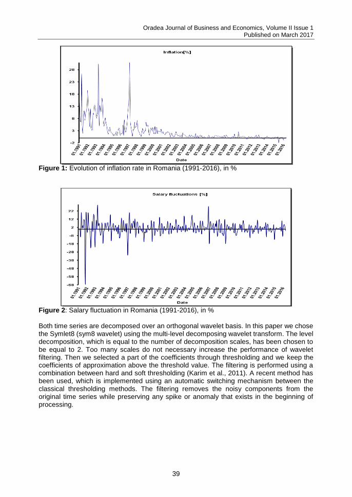
Oradea Journal of Business and Economics, Volume II Issue 1 Published on March 2017
39
Figure 1: Evolution of inflation rate in Romania (1991-2016), in %
Figure 2: Salary fluctuation in Romania (1991-2016), in % Both time series are decomposed over an orthogonal wavelet basis. In this paper we chose the Symlet8 (sym8 wavelet) using the multi-level decomposing wavelet transform. The level decomposition, which is equal to the number of decomposition scales, has been chosen to be equal to 2. Too many scales do not necessary increase the performance of wavelet filtering. Then we selected a part of the coefficients through thresholding and we keep the coefficients of approximation above the threshold value. The filtering is performed using a combination between hard and soft thresholding (Karim et al., 2011). A recent method has been used, which is implemented using an automatic switching mechanism between the classical thresholding methods. The filtering removes the noisy components from the original time series while preserving any spike or anomaly that exists in the beginning of processing.
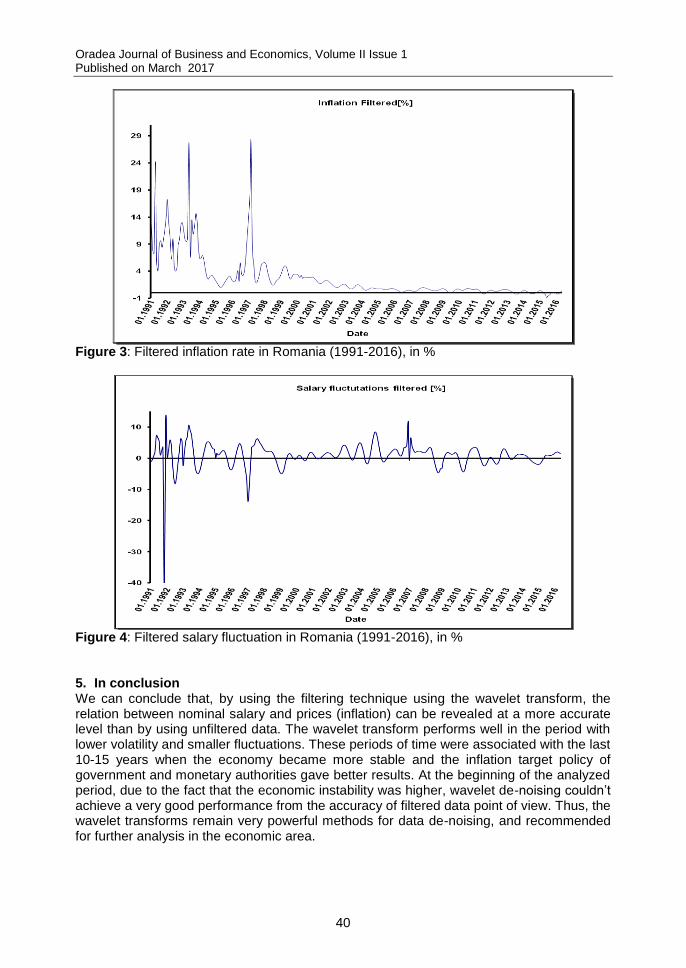
Oradea Journal of Business and Economics, Volume II Issue 1 Published on March 2017
40
Figure 3: Filtered inflation rate in Romania (1991-2016), in %
Figure 4: Filtered salary fluctuation in Romania (1991-2016), in % 5. In conclusion We can conclude that, by using the filtering technique using the wavelet transform, the relation between nominal salary and prices (inflation) can be revealed at a more accurate level than by using unfiltered data. The wavelet transform performs well in the period with lower volatility and smaller fluctuations. These periods of time were associated with the last 10-15 years when the economy became more stable and the inflation target policy of government and monetary authorities gave better results. At the beginning of the analyzed period, due to the fact that the economic instability was higher, wavelet de-noising couldn’t achieve a very good performance from the accuracy of filtered data point of view. Thus, the wavelet transforms remain very powerful methods for data de-noising, and recommended for further analysis in the economic area.
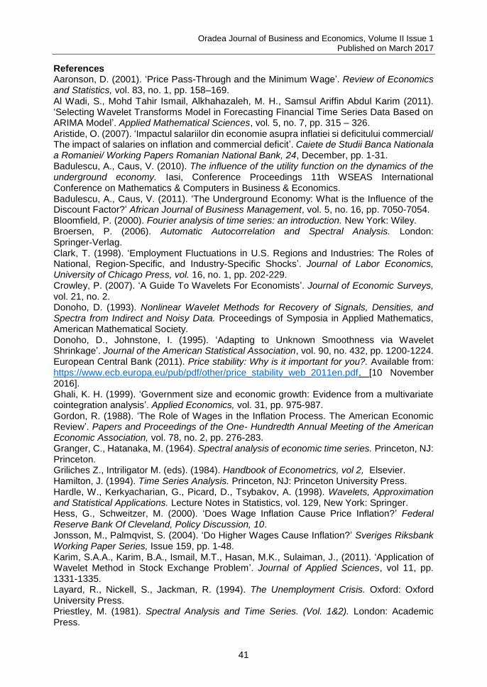
Oradea Journal of Business and Economics, Volume II Issue 1 Published on March 2017
41
References Aaronson, D. (2001). ‘Price Pass-Through and the Minimum Wage’. Review of Economics and Statistics, vol. 83, no. 1, pp. 158–169. Al Wadi, S., Mohd Tahir Ismail, Alkhahazaleh, M. H., Samsul Ariffin Abdul Karim (2011). ‘Selecting Wavelet Transforms Model in Forecasting Financial Time Series Data Based on ARIMA Model’. Applied Mathematical Sciences, vol. 5, no. 7, pp. 315 – 326. Aristide, O. (2007). ‘Impactul salariilor din economie asupra inflatiei si deficitului commercial/ The impact of salaries on inflation and commercial deficit’. Caiete de Studii Banca Nationala a Romaniei/ Working Papers Romanian National Bank, 24, December, pp. 1-31. Badulescu, A., Caus, V. (2010). The influence of the utility function on the dynamics of the underground economy. Iasi, Conference Proceedings 11th WSEAS International Conference on Mathematics & Computers in Business & Economics. Badulescu, A., Caus, V. (2011). ‘The Underground Economy: What is the Influence of the Discount Factor?’ African Journal of Business Management, vol. 5, no. 16, pp. 7050-7054. Bloomfield, P. (2000). Fourier analysis of time series: an introduction. New York: Wiley. Broersen, P. (2006). Automatic Autocorrelation and Spectral Analysis. London: Springer-Verlag. Clark, T. (1998). ‘Employment Fluctuations in U.S. Regions and Industries: The Roles of National, Region-Specific, and Industry-Specific Shocks’. Journal of Labor Economics, University of Chicago Press, vol. 16, no. 1, pp. 202-229. Crowley, P. (2007). ‘A Guide To Wavelets For Economists’. Journal of Economic Surveys, vol. 21, no. 2. Donoho, D. (1993). Nonlinear Wavelet Methods for Recovery of Signals, Densities, and Spectra from Indirect and Noisy Data. Proceedings of Symposia in Applied Mathematics, American Mathematical Society. Donoho, D., Johnstone, I. (1995). ‘Adapting to Unknown Smoothness via Wavelet Shrinkage’. Journal of the American Statistical Association, vol. 90, no. 432, pp. 1200-1224. European Central Bank (2011). Price stability: Why is it important for you?. Available from: https://www.ecb.europa.eu/pub/pdf/other/price_stability_web_2011en.pdf. [10 November 2016]. Ghali, K. H. (1999). ‘Government size and economic growth: Evidence from a multivariate cointegration analysis’. Applied Economics, vol. 31, pp. 975-987. Gordon, R. (1988). ‘The Role of Wages in the Inflation Process. The American Economic Review’. Papers and Proceedings of the One- Hundredth Annual Meeting of the American Economic Association, vol. 78, no. 2, pp. 276-283. Granger, C., Hatanaka, M. (1964). Spectral analysis of economic time series. Princeton, NJ: Princeton. Griliches Z., Intriligator M. (eds). (1984). Handbook of Econometrics, vol 2, Elsevier. Hamilton, J. (1994). Time Series Analysis. Princeton, NJ: Princeton University Press. Hardle, W., Kerkyacharian, G., Picard, D., Tsybakov, A. (1998). Wavelets, Approximation and Statistical Applications. Lecture Notes in Statistics, vol. 129, New York: Springer. Hess, G., Schweitzer, M. (2000). ‘Does Wage Inflation Cause Price Inflation?’ Federal Reserve Bank Of Cleveland, Policy Discussion, 10. Jonsson, M., Palmqvist, S. (2004). ‘Do Higher Wages Cause Inflation?’ Sveriges Riksbank Working Paper Series, Issue 159, pp. 1-48. Karim, S.A.A., Karim, B.A., Ismail, M.T., Hasan, M.K., Sulaiman, J., (2011). ‘Application of Wavelet Method in Stock Exchange Problem’. Journal of Applied Sciences, vol 11, pp. 1331-1335. Layard, R., Nickell, S., Jackman, R. (1994). The Unemployment Crisis. Oxford: Oxford University Press. Priestley, M. (1981). Spectral Analysis and Time Series. (Vol. 1&2). London: Academic Press.
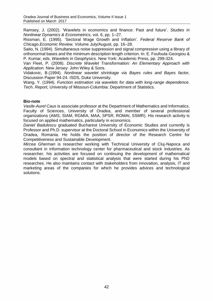
Oradea Journal of Business and Economics, Volume II Issue 1 Published on March 2017
42
Ramsey, J. (2002). ‘Wavelets in economics and finance: Past and future’. Studies in Nonlinear Dynamics & Econometrics, vol. 6, pp. 1–27. Rissman, E. (1995). ‘Sectoral Wage Growth and Inflation’. Federal Reserve Bank of Chicago.Economic Review, Volume July/August, pp. 16–28. Saito, N. (1994). Simultaneous noise suppression and signal compression using a library of orthonormal bases and the minimum description length criterion. In: E. Foufoula-Georgiou & P. Kumar, eds. Wavelets in Geophysics. New York: Academic Press, pp. 299-324. Van Fleet, P. (2008). Discrete Wavelet Transformation: An Elementary Approach with Application. New Jersey: John Wiley & Sons. Vidakovic, B.(1994). Nonlinear wavelet shrinkage via Bayes rules and Bayes factor, Discussion Paper 94-24. ISDS, Duke University. Wang, Y. (1994). Function estimation via wavelets for data with long-range dependence. Tech. Report, University of Missouri-Columbia: Department of Statistics. Bio-note Vasile-Aurel Caus is associate professor at the Department of Mathematics and Informatics, Faculty of Sciences, University of Oradea, and member of several professional organizations (AMS, SIAM, RGMIA, MAA, SPSR, ROMAI, SSMR). His research activity is focused on applied mathematics, particularly in economics. Daniel Badulescu graduated Bucharest University of Economic Studies and currently is Professor and Ph.D. supervisor at the Doctoral School in Economics within the University of Oradea, Romania. He holds the position of director of the Research Centre for Competitiveness and Sustainable Development. Mircea Gherman is researcher working with Technical University of Cluj-Napoca and consultant in information technology center for pharmaceutical and stock industries. As researcher, his activities are focused on continuing the development of mathematical models based on spectral and statistical analysis that were started during his PhD researches. He also maintains contact with stakeholders from innovation, analysis, IT and marketing areas of the companies for which he provides advices and technological solutions.
Oradea Journal of Business and Economics, Volume II Issue 1 Published on March 2017
43
THE LINK BETWEEN BANK CREDIT AND PRIVATE SECTOR INVESTMENT IN NIGERIA FROM 1980-2014
Ephraim Ugwu1
, Johnson Okoh2, Stella Mbah
3
1Department of Economics and Development Studies, Faculty of Social Sciences, Federal
University, Oye-Ekiti, Ekiti State, Nigeria. 2Department of Banking and Finance, National Open University of Nigeria, Lagos State,
Nigeria. 3Department of Economics and Development Studies, Faculty of Social Sciences, Federal
University, Oye-Ekiti, Ekiti State, Nigeria. [email protected] [email protected] [email protected] Abstract: This study attempts to investigate the link between bank credit and private sector investment in Nigeria from 1980 to 2014 using Ordinary Least Square (OLS) regression procedure. The study also employs other preliminary investigations which include, unit root, cointegration and Granger causality test procedures. The OLS result indicates that the coefficients of the variables which include, banks credit to the private sector (CRPRIVAT), trade openness (OPEN), exchange rate (EXCHR) and total bank saving (BSAVING) exhibit positive signs to the dependent variable, private investment (INVEST) during the period under review, while the coefficients of two other variables, capital expenditure (CAP) and interest rate (INTR) indicate negative signs to the dependent variable. The stationarity test result shows that all the variables under consideration are stationary and integrated of order one at 5% significance level. Also, the cointegration test result indicates at most five cointegrating equations at 5% level of significance. The Granger causality test result shows that a bi-directional causality exists between banks credit and private investment and also between private investment and capital expenditure, while a uni-directional causality exists from exchange rate to private investment.Statistically, the descriptive statistics result indicates that all the variables have a positive mean values which ranges from 18.05390 to 2427052 with 34 observations.The correlation test result obtained shows that four variables, CRPRIVAT, OPEN, EXCHR and BSAVING have positive relationships with the dependent variable INVEST. The t-statistic result shows that five of the variables which includes, CRPRIVAT, OPEN, CAP, INTR and EXCHR are statistically significant at 5% significance level. The study recommends that there is a need for increased Federal government support to banks in terms of policies that would encourage lending to the private sector in Nigeria. Keywords: Bank credit, Private investment, OLS regression, cointegration, Granger causality. JEL classification: B22, B26, E44, E50, G21, N27. 1. Introduction Banks have a strategic role to play in national development as a result of their basic function as financial intermediaries, saving mobilization especially from the surplus to sectors that are deficient. Bank credit plays an important role in the funding of capital investment in
Corresponding author
Oradea Journal of Business and Economics, Volume II Issue 1 Published on March 2017
44
Nigeria. The corporate finance structure in Nigeria has been characterized by strong bank-lending relationships. The size of the banking sectors’ assets relative to GDP determines its strategic role it plays in the economy. Banks’ assets are predominately loans and the ease with which companies can access credit is an appropriate measure for the financial sector’s contribution to economic growth, which implies that the failure of the banking system brings host implications for the real economy. Sichei and Njenga (2012) stated that monetary policy is transmitted to the real economy through different channels which are collectively known as monetary policy transmission mechanisms. There are four channels of monetary policy transmissions in any modern economy; interest rate channel, credit channel (balance-sheet and bank-lending channels), exchange rate channel and other asset (equity and real estate) prices channel. The interest rate channel is the basic transmission mechanism. Changes in the average interest rates will also have cash flow effects on borrowers and lenders (Sichei and Njenga, 2012). Banks play a pivotal role in the credit transmission channel of the economy, developed or developing, liberalised or centrally controlled. By its very nature, banking is an attempt to manage multiple and seemingly opposing needs. Banks accept deposits, by assuring savers that their deposits are liquid and secured. In recognition of the fact that a well-equipped and capitalized bank would go along in strengthening the banking sector, the CBN raised the minimum capitalization for banks from N2billion (naira) to N25 billionin 2004. The recapitalization of the country’s banking sector was aimed at establishing a diversified, strong and reliable banking sector which will ensure the safety of the depositors’ money, play active developmental roles in Nigerian economy, and be competent and competitive in the African regional and global financial system (Soludo, 2007). 1.1. Statement of the problem In Nigeria, the problem of mobilizing savings and deposits has always been the bane of economic growth and development. Savings and investment are very minimal in Nigeria due to high inflation and currency devaluations (Uremadu, 2007). As financial resources are a very vital factor in economic development, its mobilization will lead to increased capital formation. Capital formation or gross domestic investment (GDI) requires the release of domestic goods and services for real asset investment or the import of resources from outside or, as it is usually the case, a combination of the two (Uremadu, 2006). The financial mobilization problem is closely linked with savings problems, and developing countries are commonly characterized by a low rate of domestic savings. Nonetheless, gross domestic savings is still relatively reasonable in most Least Developing Countries (LDCs), but the efficiency in translating accumulated savings into productive investments is lacking. Thus the Private sector continues to face challenges in terms of asses to credit in the face of growth of the financial sector and interventions by the nation’s apex body, the Central Bank of Nigeria (CBN) in boosting liquidity. The CBN also introduced a low interest policy in order to stimulate lending to the private sector. But the deposit money banks are still reluctant to extend credit mainly due to the high risk perception in the market. The question this study tends to answer is therefore stated as follows: Does bank credit impact on private investment in Nigeria? What is the direction of causality between bank credit, other monetary policy variables and private investment growth in Nigeria? 1.2. Objectives of the study The broad objective of this study is to investigate the link between banks credit and private sector investment in Nigeria. The specific objectives are:
a. To determine the impact of other macroeconomic variables on private investment in Nigeria
b. To determine the direction of causality between bank credit, macroeconomic variables and private investment growth in Nigeria
Oradea Journal of Business and Economics, Volume II Issue 1 Published on March 2017
45
c. To proffer measures aimed at improving access to bank credit facilities by the private sector in the country.
1.3. Hypothesis of the study The research hypotheses that would guide this study is therefore stated as follows: i. There is no link between banks credit and private sector investment growth in
Nigeria ii. There is no link between other macroeconomic variables and private investment
growth in Nigeria iii. There is no direction of causality between banks credit, macroeconomic variables
and private investment in Nigeria 1.4. Scope of the study This study covers the period from 1980 to 2014.The choice of this particular period is motivated by the availability of data. 2. Literature review The role of financial services sector which involves deposit mobilization and credit supplies to the economic units of the polity is widely acknowledged in Literature .Some of these works that concern environmental factors that affect credit availability to private sector investment and the overall impact on the economy will be reviewed. Traditionally, there are four key channels of monetary policy transmission mechanism which include interest rate, credit aggregates, asset prices and exchange rate channels. Bernanke and Gertler (1995) noted interest rate channel as the dominant transmission mechanism of monetary policy. According the authors, an expansionary monetary policy is expected to lead to a lowering cost of loanable funds, which would lead to a rise in investment and consumption demand and equally be reflected in aggregate output and prices. Mohan (2008) stated that a fifth channel –expectation- has taken a prominent role in the conduct of forward looking monetary policy as a result of its influence on the traditional four channels. According to the author, the interaction between short and long run real rates is widely acknowledged to move from the expectational hypothesis of the term structure of interest rates. The expectations channel of monetary policy states that the vies of economic agents about future shocks to the economy as the central bank’s reactions can impact the variables that are determined in a forward looking approach(Mohan, 2008). Also, Knoop (2008) identifies two important features of the above mentioned channels of monetary policy transmission. First, these channels are not mutually exclusive. This means monetary policy can operate through all the channels at the same time. Second, each of these channels operates through their effect on aggregate demand and investment. When the central bank increases money supply and lowers interest rates, the profits and cash flows of borrowers increase and increase in money supply also improves the financial position of lenders by increasing liquidity and asset prices. Lenders respond to these improvements by reducing their lending rates as well as lowering other costs of credit intermediation. These lower costs of credit intermediation increase credit and spur consumption and investment. 2.1. Bank level environment According to Love and Mylenko (2003), in Sub-Saharan Africa (SSA), a sharp rise in banks’ investment in government securities has been recorded. As a result, commercial banks hold a very large part of their domestic assets in the form of government securities. The authors further argued that the increased return on government paper and bank bills provides banks with an alternative opportunity for high return low risk investment. From the supply side, securities issuance was increased through government borrowing to finance fiscal deficits.
Oradea Journal of Business and Economics, Volume II Issue 1 Published on March 2017
46
In SSA, banks plays an important role as result of their dominance in the financial systems and due to limitations of informal finance. The extent of banks’ lending especially to Small and Medium Scale Enterprises (SMEs) depend on a range of country and bank specific factors (Beck, Demirgüç – Kunt and Martinez Peria, 2011). The factors according to the authors, include macroeconomic environment, the legal and regulatory framework, the state of the financial sector infrastructure, banks internal limitations in terms of capacity utilization and technology. Other factors include SME specific factors especially the SME landscape in terms of size, number and focus of operation. The SMEs are typically more credit constrained in SSA than large firms and this affects their growth (Beck et al, 2011). A cross-country study on the drivers of bank financing according to Berg and Fuchs (2013) indicate that the share of lending to the SMEs in the overall portfolios of banks varies between ten to twenty percent. The authors noted that banks in Kenya, Rwanda and Tanzania are more involved with SMEs in terms of the share loan book moving to the SMEs than banks in Nigeria and South Africa. The most important contributing factors to banks’ lending include the structure and size of the economy, the extent of Government borrowing, the degree of innovation as regards SME lending; and the state of the financial sector infrastructure as well as the enabling environment including Government support programmes (Berg and Fuchs, 2013). 2.2. Investment in Nigeria From 2004, investment in the Nigerian economy has continuously witnessed a decline which has fallen below any other level of loss ever recorded in this sector since independence. With as low as N1921.2 million in 2005 to as drastically low as N114,484.4 million in the year 2008, the levels of domestic investment in the Nigeria economy was about 145% lower than 2004 level (Donwa and Agbontaen, 2010). The authors noted that the level of technical know-how is still very low while supply of infrastructural facilities remains inadequate. These evidence of inconsistencies in both policy prescription and prudent fiscal measures have resulted to huge capital flights. The instability in the polity have led to decline in the level of investment activities (Donwa and Agbontaen, 2010). However, in 2014 as result of rapidly growing contribution to the Nigerian economy from sectors such as telecommunication, banking and film industry, the Government rebased its Gross Domestic Product (GDP) to $510 billion (United States Dollars).Thus making the economy one of the largest in Sub-Saharan Africa. 2.3. Empirical review Sinevičienė (2015) examines relationship between government expenditure and private investment in the case of small open economies using cross-correlations and Granger causality tests on time series data of Bulgaria, Estonia, Latvia, Lithuania and Slovenia from 1996 – 2012. The results show that impact of public spending increase on private investment is very weak except in the case of Bulgaria. The study also notes that the impact of private investment increase on public spending is very different in analyzed countries. Omorokunwa and Ikponmwosa (2014) investigate the dynamic relationship between exchange rate volatility and foreign private investment in Nigeria from 1980 to 2011. Using Error Correction Model (ECM) techniques, the result shows that exchange rate shows negative effect on Foreign Direct Investment (FDI) to Nigeria. The result shows a strong positive effect on portfolio in the long run. Zardashty (2014) analyze the impacts of real exchange rate on private sector investment in Iran from 1961-2008 using an EGARCH model. The results indicate that the index of real exchange rate has a negative effect on private investment, GDP ratio, and imports of capital commodity. The result equally indicates that inflation have negative effects on private investment to GDP ratio.
Oradea Journal of Business and Economics, Volume II Issue 1 Published on March 2017
47
Oyieke (2011) examines the relationship between public investment and it’s financing on private sector investment in Kenya from 1964 to 2006. Using an error correction framework and time series data for the fiscal years 1964-2006, the study indicates that agricultural investment has a significant positive effect on private investment and domestic debt has a negative effect. Rahila, Rehmat and Zakir (2010) examine long run and short run relationship between private investment, savings, real interest rate on Bank deposits and Bank Credit to the private sector in Pakistan for the period 1973 to 2007. Applying ARDL Bounds Testing Approach, the results show that Private Investment is positively affected by Savings, Real interest rate on bank deposits, Bank credit to private sector and Public investment in the long run. 3. Methodology of the research 3.1. Sources of data The research utilizes data generated from the Central Bank of Nigeria statistical bulletin on private sector investment, data on total bank savings, interest rate, exchange rate, trade openness, government capital expenditure and total bank credit to private sector from 1980-2014. 3.2. Data analysis method The study employed OLS regression for the data analysis. The private investment is the dependent variable, while, banks credit, trade openness, capital expenditure, interest rate, exchange rate and bank saving, are the independent variables. The model for the impact of banks credit on private investment in Nigeria could be stated as follows: 3.3. Model specification
INVEST =( CRPRIVAT, OPEN, CAP, INTR, EXCHR, BSAVING)………………..(1)
SET DEFINITION INVEST = private investment CRPRIVAT = Banks credit to the private sector OPEN= Trade openness CAP= Federal capital expenditure INTR = Interest rate EXCHR= Exchange rate BSAING= Total bank saving Assuming a linear relationship between the dependent variable and independent variables, and using the multiple regression model can be specified as follows:
0 1 2 3 4 5 6 tINVEST = + CRPRIVAT+ OPEN+ CAP+ INTR+ EXCHR+ BSAVING + (2)
where t = Error term
3.4. Estimation Procedures Unit root test To test for stationarity is done using the Augmented Dickey Fuller test (ADF). The ADF test equation is specified as follows:
1 1
1
k
t t t t
i
u u u
……………………………………..……..………..(3)
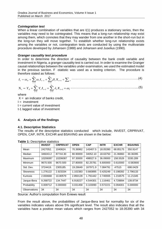
Oradea Journal of Business and Economics, Volume II Issue 1 Published on March 2017
48
Cointegration test When a linear combination of variables that are I(1) produces a stationary series, then the variables may need to be cointegrated. This means that a long-run relationship may exist among them, which connotes that they may wander from one another in the short-run but in the long-run they will move together. To establish whether long-run relationship exists among the variables or not, cointegration tests are conducted by using the multivariate procedure developed by Johansen (1988) and Johansen and Juselius (1990).
Granger causality test procedure In order to determine the direction of causality between the bank credit variable and investment in Nigeria, a granger causality test is carried out. In order to examine the Granger causal relationships between the variables under examination, we used the estimated model in the previous section. F -statistic was used as a testing criterion. The procedure is therefore stated as follows:
1 2
0 1 1
1 1
k k
t i t i t t
i i
I I X
……………………………………………………….(4)
3 4
t 0 1 1
1 1
Xk k
i t i t t
i i
I X
.……………………………………………….……....(5)
where X = an indicator of banks credit, I = investment t = current value of investment t-1 lagged value of investment 4. Analysis of the findings
4.1. Descriptive Statistics The results of the descriptive statistics conducted which include, INVEST, CRPRIVAT, OPEN, CAP, INTR, EXCHR and BSAVING are shown in the below: Table 1: Descriptive statistics
INVEST CRPRIVAT OPEN CAP INTR EXCHR BSAVING
Mean 2427052. 1040624. 70.36962 143407.5 18.05390 68.85175 350.9147
Median 346043.2 87744.30 80.90000 34052.10 18.63750 21.96860 30.36395
Maximum 10206087 10206087 97.30000 498027.6 36.09000 158.5526 3330.289
Minimum 9670.500 9670.500 27.80000 82.25781 6.600000 0.610000 -0.583900
Std. Dev. 3724419. 2305185. 19.26649 167971.9 7.084791 .47515 698.0429
Skewness 1.276122 2.923334 1.102383 0.660895 0.425249 0.198392 2.796133
Kurtosis 2.830668 10.80579 2.850128 1.791442 2.745555 1.216575 11.21345
Jarque-Bera 9.268722 134.7447 6.918227 4.544301 1.116461 4.728894 139.8734
Probability 0.009712 0.000000 0.031458 0.103090 0.572221 0.094001 0.000000
Observations 34 34 34 34 34 34 34
Source: Author’s computation from Eviews result From the result above, the probabilities of Jarque-Bera test for normality for six of the variables indicates values above 5% significant level. The result also indicates that all the variables have a positive mean values which ranges from 2427052 to 18.05390 with 34
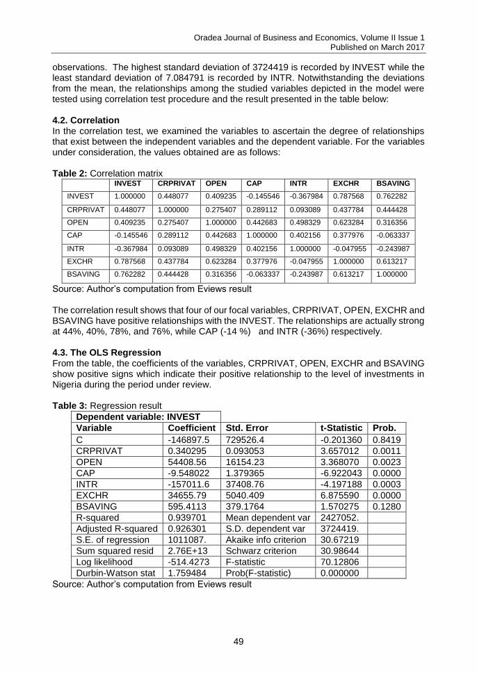
Oradea Journal of Business and Economics, Volume II Issue 1 Published on March 2017
49
observations. The highest standard deviation of 3724419 is recorded by INVEST while the least standard deviation of 7.084791 is recorded by INTR. Notwithstanding the deviations from the mean, the relationships among the studied variables depicted in the model were tested using correlation test procedure and the result presented in the table below: 4.2. Correlation In the correlation test, we examined the variables to ascertain the degree of relationships that exist between the independent variables and the dependent variable. For the variables under consideration, the values obtained are as follows: Table 2: Correlation matrix
INVEST CRPRIVAT OPEN CAP INTR EXCHR BSAVING
INVEST 1.000000 0.448077 0.409235 -0.145546 -0.367984 0.787568 0.762282
CRPRIVAT 0.448077 1.000000 0.275407 0.289112 0.093089 0.437784 0.444428
OPEN 0.409235 0.275407 1.000000 0.442683 0.498329 0.623284 0.316356
CAP -0.145546 0.289112 0.442683 1.000000 0.402156 0.377976 -0.063337
INTR -0.367984 0.093089 0.498329 0.402156 1.000000 -0.047955 -0.243987
EXCHR 0.787568 0.437784 0.623284 0.377976 -0.047955 1.000000 0.613217
BSAVING 0.762282 0.444428 0.316356 -0.063337 -0.243987 0.613217 1.000000
Source: Author’s computation from Eviews result The correlation result shows that four of our focal variables, CRPRIVAT, OPEN, EXCHR and BSAVING have positive relationships with the INVEST. The relationships are actually strong at 44%, 40%, 78%, and 76%, while CAP (-14 %) and INTR (-36%) respectively. 4.3. The OLS Regression From the table, the coefficients of the variables, CRPRIVAT, OPEN, EXCHR and BSAVING show positive signs which indicate their positive relationship to the level of investments in Nigeria during the period under review. Table 3: Regression result
Dependent variable: INVEST
Variable Coefficient Std. Error t-Statistic Prob.
C -146897.5 729526.4 -0.201360 0.8419
CRPRIVAT 0.340295 0.093053 3.657012 0.0011
OPEN 54408.56 16154.23 3.368070 0.0023
CAP -9.548022 1.379365 -6.922043 0.0000
INTR -157011.6 37408.76 -4.197188 0.0003
EXCHR 34655.79 5040.409 6.875590 0.0000
BSAVING 595.4113 379.1764 1.570275 0.1280
R-squared 0.939701 Mean dependent var 2427052.
Adjusted R-squared 0.926301 S.D. dependent var 3724419.
S.E. of regression 1011087. Akaike info criterion 30.67219
Sum squared resid 2.76E+13 Schwarz criterion 30.98644
Log likelihood -514.4273 F-statistic 70.12806
Durbin-Watson stat 1.759484 Prob(F-statistic) 0.000000
Source: Author’s computation from Eviews result
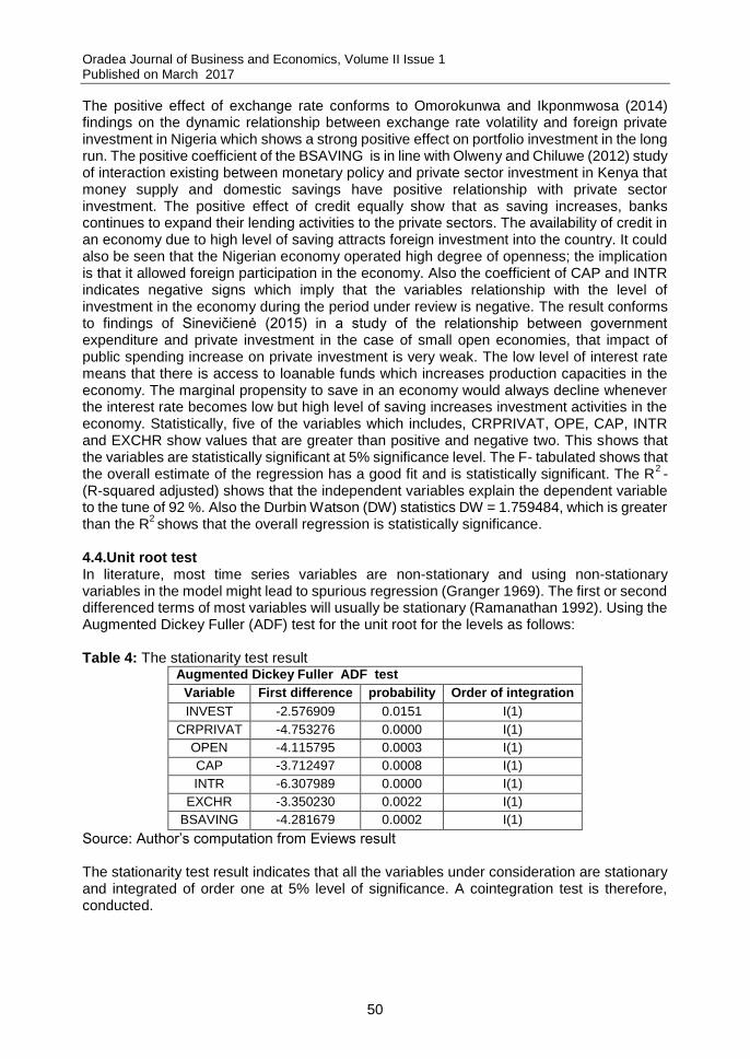
Oradea Journal of Business and Economics, Volume II Issue 1 Published on March 2017
50
The positive effect of exchange rate conforms to Omorokunwa and Ikponmwosa (2014) findings on the dynamic relationship between exchange rate volatility and foreign private investment in Nigeria which shows a strong positive effect on portfolio investment in the long run. The positive coefficient of the BSAVING is in line with Olweny and Chiluwe (2012) study of interaction existing between monetary policy and private sector investment in Kenya that money supply and domestic savings have positive relationship with private sector investment. The positive effect of credit equally show that as saving increases, banks continues to expand their lending activities to the private sectors. The availability of credit in an economy due to high level of saving attracts foreign investment into the country. It could also be seen that the Nigerian economy operated high degree of openness; the implication is that it allowed foreign participation in the economy. Also the coefficient of CAP and INTR indicates negative signs which imply that the variables relationship with the level of investment in the economy during the period under review is negative. The result conforms to findings of Sinevičienė (2015) in a study of the relationship between government expenditure and private investment in the case of small open economies, that impact of public spending increase on private investment is very weak. The low level of interest rate means that there is access to loanable funds which increases production capacities in the economy. The marginal propensity to save in an economy would always decline whenever the interest rate becomes low but high level of saving increases investment activities in the economy. Statistically, five of the variables which includes, CRPRIVAT, OPE, CAP, INTR and EXCHR show values that are greater than positive and negative two. This shows that the variables are statistically significant at 5% significance level. The F- tabulated shows that the overall estimate of the regression has a good fit and is statistically significant. The R
2 -
(R-squared adjusted) shows that the independent variables explain the dependent variable to the tune of 92 %. Also the Durbin Watson (DW) statistics DW = 1.759484, which is greater than the R
2 shows that the overall regression is statistically significance.
4.4.Unit root test In literature, most time series variables are non-stationary and using non-stationary variables in the model might lead to spurious regression (Granger 1969). The first or second differenced terms of most variables will usually be stationary (Ramanathan 1992). Using the Augmented Dickey Fuller (ADF) test for the unit root for the levels as follows: Table 4: The stationarity test result
Augmented Dickey Fuller ADF test
Variable First difference probability Order of integration
INVEST -2.576909 0.0151 I(1)
CRPRIVAT -4.753276 0.0000 I(1)
OPEN -4.115795 0.0003 I(1)
CAP -3.712497 0.0008 I(1)
INTR -6.307989 0.0000 I(1)
EXCHR -3.350230 0.0022 I(1)
BSAVING -4.281679 0.0002 I(1)
Source: Author’s computation from Eviews result The stationarity test result indicates that all the variables under consideration are stationary and integrated of order one at 5% level of significance. A cointegration test is therefore, conducted.
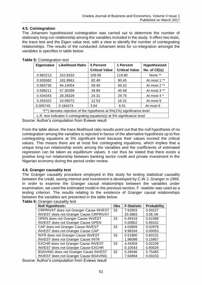
Oradea Journal of Business and Economics, Volume II Issue 1 Published on March 2017
51
4.5. Cointegration The Johansen hypothesized cointegration was carried out to determine the number of stationary long-run relationship among the variables included in the study. It offers two tests, the trace test and the Eigen value test, with a view to identify the number of cointegrating relationships. The results of the conducted Johansen tests for co-integration amongst the variables is specifies in table below: Table 5: Cointegration test
Eigenvalue Likelihood Ratio 5 Percent
Critical Value
1 Percent
Critical Value
Hypothesized
No. of CE(s)
0.982213 310.8333 109.99 119.80 None **
0.935582 181.8961 82.49 90.45 At most 1 **
0.683736 94.14054 59.46 66.52 At most 2 **
0.596211 57.30289 39.89 45.58 At most 3 **
0.434343 28.28329 24.31 29.75 At most 4 *
0.265322 10.05072 12.53 16.31 At most 5
0.005745 0.184374 3.84 6.51 At most 6
*(**) denotes rejection of the hypothesis at 5%(1%) significance level
L.R. test indicates 5 cointegrating equation(s) at 5% significance level
Source: Author’s computation from Eviews result From the table above, the trace likelihood ratio results point out that the null hypothesis of no cointegration among the variables is rejected in favour of the alternative hypothesis up to five cointegrating equations at 5% significant level because their values exceed the critical values. This means there are at most five cointegrating equations, which implies that a unique long-run relationship exists among the variables and the coefficients of estimated regression can be taken as equilibrium values. It can thus be stated that there exists a positive long run relationship between banking sector credit and private investment in the Nigerian economy during the period under review. 4.6. Granger causality test The Granger causality procedure employed in this study for testing statistical causality between the credit, saving interest and investment is developed by C.W.J. Granger in 1969. In order to examine the Granger causal relationships between the variables under examination, we used the estimated model in the previous section. F -statistic was used as a testing criterion. The results relating to the existence of Granger causal relationships between the variables are presented in the table below: Table 6: Granger causality test
Null Hypothesis: Obs F-Statistic Probability
CRPRIVAT does not Granger Cause INVEST INVEST does not Granger Cause CRPRIVAT
33 7.62803 20.3683
0.00227 3.5E-06
OPEN does not Granger Cause INVEST INVEST does not Granger Cause OPEN
33 0.49319 0.00852
0.61588 0.99152
CAP does not Granger Cause INVEST INVEST does not Granger Cause CAP
33 4.03809 9.98334
0.02878 0.00053
INTR does not Granger Cause INVEST INVEST does not Granger Cause INTR
33 0.51800 1.96098
0.60131 0.15957
EXCHR does not Granger Cause INVEST INVEST does not Granger Cause EXCHR
33 4.44304 0.10543
0.02109 0.90029
BSAVING does not Granger Cause INVEST INVEST does not Granger Cause BSAVING
32 0.28446 7.64894
0.75465 0.00233
Source: Author’s computation from Eviews result
Oradea Journal of Business and Economics, Volume II Issue 1 Published on March 2017
52
The results given above suggest that there exists a bi-directional causality between banks credit and private investment. There is no direction of causality between trade openness and private investment. The study shows that there is bi-directional causality between private investment and capital expenditure. The result table indicates no direction of causality between interest rate and private investment. The result equally indicates that there is a uni-directional causality from exchange rate to private investment. A uni-directional causality exists from private investment to bank saving. 5. Conclusion It has been noted that credit plays an important role in the funding of new investments in Nigeria. Monetary policy is transmitted to the real economy through different channels which are collectively known as monetary policy transmission mechanisms. The OLS regression result obtained shows that the coefficients of the variables, CRPRIVAT, OPEN, EXCHR and BSAVING show positive signs which indicates their positive relationship to the level of investments in Nigeria during the period under review. Also the coefficient of CAP and INTR indicates negative signs which imply that the variables relationship with the level of investment in the economy during the period under review is negative. Statistically, the t-statistic result shows that five of the variables which includes, CRPRIVAT, OPE, CAP, INTR and EXCHR are statistically significant at 5% significance level. The stationarity test result obtained indicates that all the variables under consideration are stationary and integrated of order one at 5% level of significance. The Johansen hypothesized cointegration test result shows that the trace likelihood ratio results point out that the null hypothesis of no cointegration among the variables is rejected in favour of the alternative hypothesis up to five cointegrating equations at 5% significant level. The Granger causality procedure conducted indicates that there exists a bi-directional causality between banks credit and private investment; also, there is bi-directional causality between private investment and capital expenditure. While a uni-directional causality exists from exchange rate to private investment. Furthermore, the positive relationship between bank credit to the private sector variable, (CRPRIVAT) and the private investment in Nigeria during the period under review ensures that the major objective of the study which is to investigate the link between banks credit and private sector investment in Nigeria has been achieved; and as result, we accept the hypothesis that there is a link between banks credit and private sector investment growth in Nigeria. The study therefore recommends that there is a need for increased Federal government support to banks in terms of policies that would encourage lending to private sector in Nigeria. Banks should place more emphasis on human capacity building to ensure funding of viable projects for enhanced economic growth and development. The Central Bank should focus on market driven interest rate regime in order to encourage savings as well as boosting investment activities in the country. References Beck, T., Demirgüç -Kunt, A., Martinez Peria, M. (2011). ‘Bank financing for SMEs: Evidence across countries and bank-ownership types’. Journal of Financial Services, Vol. 39, pp. 35–54. Berg, G., Fuchs, M. (2013). ‘Bank Financing of SMEs in Five Sub-Saharan African Countries: The Role of Competition, Innovation, and the Government’, The World Bank Policy Research Working Paper 6563.
Oradea Journal of Business and Economics, Volume II Issue 1 Published on March 2017
53
Bernanke, B., Gertler, M. (1995). ‘Inside the black box: the credit channel of monetary policy transmission’, Journal of Economic Perspectives, vol. 9, no. 4. Available from: http://www.nber.org/papers/w5146. [02.02.2017] Donwa, P., Agbontaen, O.O. (2010). ‘Trends and dynamics of the determinants of investment in Nigeria’, International Review of Business Research Papers, vol. 6, no. 6, pp. 153 –163. Granger, C. W. J. (1969). ‘Investigating Causal Relationship by Econometric models and Gross-spectral Methods’, Econometrics, vol. 37, no 3, pp. 242-238. Johansen, S. (1988). ‘Statistical analysis of cointegration vectors’, Journal of Economic Dynamics and Control, vol. 12, pp. 231-54. Johansen, S., Juselius, K. (1990). ‘Maximum likelihood estimation and inference on cointegration with applications to the demand for money’, Oxf. Bull. Econ. Stat. vol. 52, pp. 169-210. Knoop, T. (2008). Modern Financial Macroeconomics: Panics, Crashes, and Crises, Wiley Blackwell publishing. Love, I., Mylenko, N. (2003). ‘Credit reporting and financing constraints’, World Bank Policy Research, Working Paper No. 3142. Mohan, R. (2008). ‘Monetary policy transmission in India’, BIS working papers no 35. Available from: http://www.bis.org/publ/bppdf/bispap35m.pdf. [02.02.2017] Olweny, T., Chiluwe, M. (2012). ‘The Effect of Monetary Policy on Private Sector Investment in Kenya’, Journal of Applied Finance & Banking, vol. 2, no. 2, pp. 239-287. Omorokunwa, O.G., Ikponmwosa, N. (2014). ‘Exchange Rate Volatility and Foreign Private Investment in Nigeria’, Asian Journal of Business Management, vol. 6, no. 4, pp. 146-154. Oyieke, S. O. (2011). ‘Government Capital Spending and Financing and its Impact on Private Investment in Kenya: 1964-2006’, African Economic Research Consortium, Nairobi, Research Paper No. 236. Sacerdoti, E. (2005). ‘Access to Bank Credit in Sub-Saharan Africa: Key Issues and Reform Strategies’, International Monetary Fund, Monetary and Financial Systems Department, Working Paper WP/05/166. Ramanathan, R. (1992). Introductory Econometrics with Applications, Second Edition. Harcourt New York, Brace Jovanovich. Sichei, M.M., Njenga G. (2012). ‘Does Bank Lending Channel Exist in Kenya: Bank Level Panel Data Analysis’, African Economic Research Consortium Research Paper 249. Available online from http://aercafrica.org/index.php/publications/view_document/346-does-bank-lending-channel-exist-in-kenya-bank-level-panel-data-analysis. [02.02.2017] Sinevičienė L.(2015). ‘Testing the Relationship between Government Expenditure and Private Investment: The Case of Small Open Economies’, Journal of Economics, Business and Management, vol. 3, no. 6. pp. 1-2. Soludo, C. C. (2007). ‘Monetary and Financial Sector Developments in Nigeria’; available from CBN website: www.cenbank.org. [02.02.2017] Rahila, M., Rehmat U. A., Zakir, H. (2010). ‘Investment, Savings, Interest Rate and Bank Credit to the Private Sector Nexus in Pakistan’, International Journal of Marketing Studies, vol.2, no.1, pp. 1-2. Uremadu, S.O. (2007). ‘Core Determinants of Financial Savings in Nigeria: An Empirical Analysis for National Monetary Policy Formulation’, International Review of Business Research Papers, pp. 356-367. Uremadu, S.O.(2006).‘The Impact of Real Interest Rate on Savings Mobilization in Nigeria’; An Unpublished Ph.D thesis, cited in Uremadu, S.O.(2011) ‘Foreign Direct Investment, Liquidity and Real Country Growth Evidence From Nigeria’, International Review of Business Research Papers, vol. 7, no. 3, pp. 170 -193.
Oradea Journal of Business and Economics, Volume II Issue 1 Published on March 2017
54
Zardashty, G. R. (2014). ‘The impact of real exchange rate uncertainty on private investment in Iran’, Kuwait Chapter of Arabian Journal of Business and Management Review, vol.3, no.10, pp.1-2. Bio-note Ugwu Ephraim is currently an Assistant Lecturer at the Federal University, Oye Ekiti (FUOYE), Ekiti State, Nigeria. He was previously a Project Manager at the Innovation and Research Centre, FUOYE. He studied Economics at the University of Nigeria, Nsukka and graduated with Bachelor of Science degree in Economics with Second Class Upper division and a Master of Science degree in Economics (Public Finance). As a researcher, Mr. Ephraim's interest is focused on issues relating to public finance and developments especially in the developing economies. Okoh Johnson holds a PhD in Banking and Finance from Nnamdi Azikiwe University, Awka Anambra State, Nigeria. He has a master’s degree in Banking and Finance and holds a B.Sc in Accountancy (2nd Class Upper Division). He had over 10years practical banking experience before he joined academics in 2012. He lectures Accounting, Banking & Finance in the University. Mbah Stella is a Lecturer 11 with the Department of Economic and Development Studies in Federal University Oye-Ekiti, Ekiti State, Nigeria. She holds a master’s degree in Economics and her research field is in Development Economics.
Oradea Journal of Business and Economics, Volume II Issue 1 Published on March 2017
55
THE STRUCTURAL EVOLUTION OF THE BANKING SYSTEM IN ROMANIA UNDER THE IMPACT OF FDI
Vasile Cocriş1, Maria-Ramona Sârbu
2 1,2
Department of Finance, Money and Public Administration, Faculty of Economics and Business Administration, „Alexandru Ioan Cuza” University of Iasi, Iasi, Romania [email protected] [email protected] Abstract: Foreign banks represent important channels for the transfer of productive resources, managerial and organizational skills and experience accumulated on international level, which led to increased competition in the banking market in Romania, which contributed to some extent to the profitability of the Romanian banking sector. The purpose of the current attempt of research is the analysis of the structural evolution of the banking sector in Romania, under the impact of foreign direct investments (FDI). Analyzing the structural evolution of the Romanian banking sector, there can be observed that in 2015, FDI has influenced some important merger operations on a level with branches of foreign banks in Romania, and over 85% of the total capital of the banking system in our country belongs to credit institutions with foreign majority ownership and to their branches. Regarding the origin of the foreign capital of credit institutions, it originates from the member states of the European Union (EU). It is also worthy of note that in 2015, the top ten banks in the banking sector of Romania held 71.6% of the assets, while the remaining 26 banks held a share of only 28.4% of the market. Banca Comercială Română, BRD - Groupe Société Générale and Banca Transilvania are in 2015 the main banks in the Romanian banking system, with a major market share. Keywords: credit institutions, market share, Herfindahl – Hirschman Index, profitability, structural developments. JEL classification: F21, G21, G31.
1. Introduction In the last years, the entrance on the market of foreign banks has contributed to the development and progress of the Romanian banking system, thus fulfilling an important role in the Romanian economy. In this context, the purpose of the current paper is the analysis of the structural evolution of the banking sector in Romania, under the impact of FDI. Because of the globalization phenomenon and the growing financial integration, many foreign banks have entered the market of developing countries. Although most foreign banks are coming from countries with a high income, recently the banks in developing countries have followed their example (Van Horen, 2007). The availability of resources and the international experience already gained by the mother-banks have a positive effect on their decision to carry out direct investment abroad (Mutinelli and Piscitello, 2001). Thus, an increasing share of the banking sector is controlled by foreign capital in most crossover countries, where on average, foreign owned banks are more efficient than domestic owned banks (Weill, 2003). Simpasa (2013), evaluates the degree of competition in the Zambian banking sector, using the Panzar-Rosse H-statistic and the Lerner Index, as a way to
Corresponding author
Oradea Journal of Business and Economics, Volume II Issue 1 Published on March 2017
56
measure competition. The findings of the study show that the entry of foreign banks and privatisation of the state-owned bank can intensify competitive pressures in the banking industry. Banks appear beyond frontiers also because economies differ in their endowment with production factors and in the efficiency of their banking sectors. From this perspective, international connections between banks played a crucial role in today’s global economy (Niepmann, 2015). To the boost of FDI activity have also contributed the lower costs of the local credit and the increase of local competition between local banks in each country through the deregulation of the interstate banking (Kandilov et. al., 2016). As foreign banks are more competitive than local banks, the entry of the foreign capital in the banking sector is important through its contribution in creating the competitive nature of the market (Mulyaningsih et. al., 2015). In this context, Morutan and Badulescu (2016) also point out that the entry is relevant for the development of the banks, but less than in the previous period, when banks entered the emerging markets of the Central and Eastern European (CEE) countries. Thus, many CEE economies are characterized by a very competitive position and successful corporate sectors, supported by a very high level of FDI penetration (Popovici, 2013: 571). Balaj (2015), compared financial performance of the domestic and foreign banks in the banking sector of Kosovo during the period of 2001-2007, using the DuPont financial analysis model in order to measure the comparative performance between domestic and foreign banks. The results from the research study showed, that foreign banks had been more efficient and profitable, thus having a higher ratio of Return on Assets (ROA) and Return on Equity (ROE), outlining that the foreign banks’ high ratio of Return on Equity is a result of a higher interest margin, which suggest that foreign banks have made a better costs management and a larger use regarding financial leverage. Ghosh (2016), using data on MENA banks for 2000-2012, examines how foreign bank presence impacts domestic bank performance. The author also analysis and the impact of foreign banks on the growth of domestic countries and its implications regarding the allocation of capital and labor. The findings suggest that foreign presence exerts significant spillover effects and increased foreign banks appear to impel domestic banks to cut back lending. Regarding its impact on growth, the results show that although labor does not exert any visible effect on GDP growth, capital exerts a positive impact on output but only when foreign bank entrance is high. In the Romanian banking system foreign banks contributed to increase efficiency in the overall banking system, therefore, the Romanian government authorities should encourage the entry of new foreign banks (Andries et. al., 2013: 195). Regarding the structure of this paper, besides the introductive chapter, the paper is structured in the following sections: section two provides an analysis regarding the structural evolution of the banking system in Romania under the impact of FDI, while the third section of the paper presents the performance of the banking sector in terms of profitability, followed by the main conclusions. 2. The structural evolution of the banking system in Romania under the impact of FDI The integration of Romania to the European Union attracted several financial groups from the community space, which considered that the local business environment is suitable to open their units in our country. From this perspective, Romania, as a member of the EU, had a high growth potential, concerning the banking sector, context in which foreign banks moved to grow along with the market. The increasing competition in the banking market and the significant entry of foreign capital have turned Romania in one of the major markets facing actors of European size (Spulbar and Nitoi, 2012: 460-461). The banking sector has played a determining role in Romania’s transition process to the market economy, given that it mediates the interface between the real economy and the nominal economy, shifting to the institutionalized mechanisms of competition. The entry of foreign capital in the banking sector in Romania was carried out through the following: (a) the
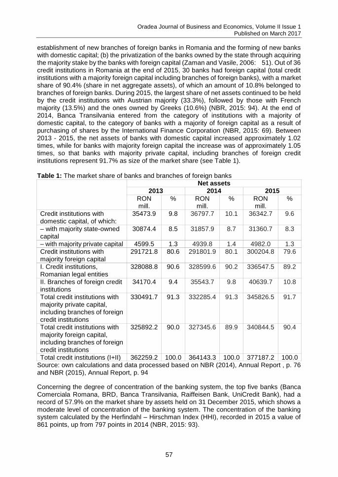
Oradea Journal of Business and Economics, Volume II Issue 1 Published on March 2017
57
establishment of new branches of foreign banks in Romania and the forming of new banks with domestic capital; (b) the privatization of the banks owned by the state through acquiring the majority stake by the banks with foreign capital (Zaman and Vasile, 2006: 51). Out of 36 credit institutions in Romania at the end of 2015, 30 banks had foreign capital (total credit institutions with a majority foreign capital including branches of foreign banks), with a market share of 90.4% (share in net aggregate assets), of which an amount of 10.8% belonged to branches of foreign banks. During 2015, the largest share of net assets continued to be held by the credit institutions with Austrian majority (33.3%), followed by those with French majority (13.5%) and the ones owned by Greeks (10.6%) (NBR, 2015: 94). At the end of 2014, Banca Transilvania entered from the category of institutions with a majority of domestic capital, to the category of banks with a majority of foreign capital as a result of purchasing of shares by the International Finance Corporation (NBR, 2015: 69). Between 2013 - 2015, the net assets of banks with domestic capital increased approximately 1.02 times, while for banks with majority foreign capital the increase was of approximately 1.05 times, so that banks with majority private capital, including branches of foreign credit institutions represent 91.7% as size of the market share (see Table 1).
Table 1: The market share of banks and branches of foreign banks
Net assets 2013 2014 2015
RON mill.
% RON mill.
% RON mill.
%
Credit institutions with domestic capital, of which:
35473.9 9.8
36797.7 10.1 36342.7 9.6
– with majority state-owned capital
30874.4 8.5 31857.9 8.7 31360.7 8.3
– with majority private capital 4599.5 1.3 4939.8 1.4 4982.0 1.3 Credit institutions with majority foreign capital
291721.8 80.6 291801.9 80.1 300204.8 79.6
I. Credit institutions, Romanian legal entities
328088.8 90.6 328599.6 90.2 336547.5 89.2
II. Branches of foreign credit institutions
34170.4 9.4 35543.7 9.8 40639.7 10.8
Total credit institutions with majority private capital, including branches of foreign credit institutions
330491.7 91.3 332285.4 91.3 345826.5 91.7
Total credit institutions with majority foreign capital, including branches of foreign credit institutions
325892.2 90.0 327345.6 89.9 340844.5 90.4
Total credit institutions (I+II) 362259.2 100.0 364143.3 100.0 377187.2 100.0 Source: own calculations and data processed based on NBR (2014), Annual Report , p. 76 and NBR (2015), Annual Report, p. 94
Concerning the degree of concentration of the banking system, the top five banks (Banca Comerciala Romana, BRD, Banca Transilvania, Raiffeisen Bank, UniCredit Bank), had a record of 57.9% on the market share by assets held on 31 December 2015, which shows a moderate level of concentration of the banking system. The concentration of the banking system calculated by the Herfindahl – Hirschman Index (HHI), recorded in 2015 a value of 861 points, up from 797 points in 2014 (NBR, 2015: 93).
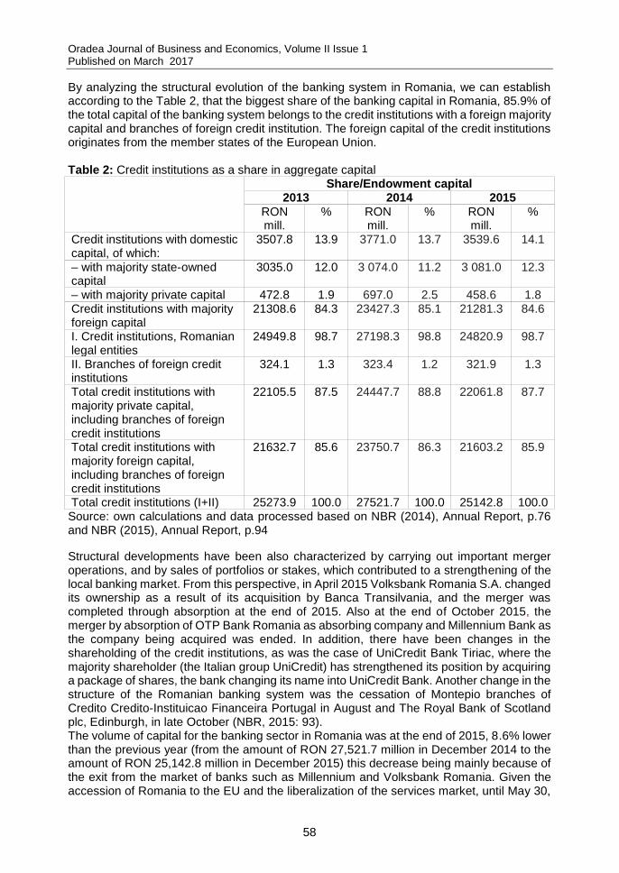
Oradea Journal of Business and Economics, Volume II Issue 1 Published on March 2017
58
By analyzing the structural evolution of the banking system in Romania, we can establish according to the Table 2, that the biggest share of the banking capital in Romania, 85.9% of the total capital of the banking system belongs to the credit institutions with a foreign majority capital and branches of foreign credit institution. The foreign capital of the credit institutions originates from the member states of the European Union.
Table 2: Credit institutions as a share in aggregate capital
Share/Endowment capital 2013 2014 2015
RON mill.
% RON mill.
% RON mill.
%
Credit institutions with domestic capital, of which:
3507.8 13.9 3771.0 13.7 3539.6 14.1
– with majority state-owned capital
3035.0 12.0 3 074.0 11.2 3 081.0 12.3
– with majority private capital 472.8 1.9 697.0 2.5 458.6 1.8 Credit institutions with majority foreign capital
21308.6 84.3 23427.3 85.1 21281.3 84.6
I. Credit institutions, Romanian legal entities
24949.8 98.7 27198.3 98.8 24820.9 98.7
II. Branches of foreign credit institutions
324.1 1.3 323.4 1.2 321.9 1.3
Total credit institutions with majority private capital, including branches of foreign credit institutions
22105.5 87.5 24447.7 88.8 22061.8 87.7
Total credit institutions with majority foreign capital, including branches of foreign credit institutions
21632.7 85.6 23750.7 86.3 21603.2 85.9
Total credit institutions (I+II) 25273.9 100.0 27521.7 100.0 25142.8 100.0 Source: own calculations and data processed based on NBR (2014), Annual Report, p.76 and NBR (2015), Annual Report, p.94
Structural developments have been also characterized by carrying out important merger operations, and by sales of portfolios or stakes, which contributed to a strengthening of the local banking market. From this perspective, in April 2015 Volksbank Romania S.A. changed its ownership as a result of its acquisition by Banca Transilvania, and the merger was completed through absorption at the end of 2015. Also at the end of October 2015, the merger by absorption of OTP Bank Romania as absorbing company and Millennium Bank as the company being acquired was ended. In addition, there have been changes in the shareholding of the credit institutions, as was the case of UniCredit Bank Tiriac, where the majority shareholder (the Italian group UniCredit) has strengthened its position by acquiring a package of shares, the bank changing its name into UniCredit Bank. Another change in the structure of the Romanian banking system was the cessation of Montepio branches of Credito Credito-Instituicao Financeira Portugal in August and The Royal Bank of Scotland plc, Edinburgh, in late October (NBR, 2015: 93). The volume of capital for the banking sector in Romania was at the end of 2015, 8.6% lower than the previous year (from the amount of RON 27,521.7 million in December 2014 to the amount of RON 25,142.8 million in December 2015) this decrease being mainly because of the exit from the market of banks such as Millennium and Volksbank Romania. Given the accession of Romania to the EU and the liberalization of the services market, until May 30,
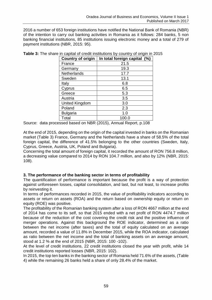
Oradea Journal of Business and Economics, Volume II Issue 1 Published on March 2017
59
2016 a number of 653 foreign institutions have notified the National Bank of Romania (NBR) of the intention to carry out banking activities in Romania as it follows: 284 banks, 5 non banking financial institutions, 85 institutions issuing electronic money and a total of 279 of payment institutions (NBR, 2015: 95).
Table 3: The share in capital of credit institutions by country of origin in 2015
Country of origin In total foreign capital (%)
France 21.5 Germany 19.3 Netherlands 17.7 Sweden 13.1 Italy 6.8 Cyprus 6.5 Greece 5.3 Austria 3.5 United Kingdom 3.0 Poland 2.3 Bulgaria 1.0 Total 100.0
Source: data processed based on NBR (2015), Annual Report, p.108 At the end of 2015, depending on the origin of the capital invested in banks on the Romanian market (Table 3) France, Germany and the Netherlands have a share of 58.5% of the total foreign capital, the difference of 41.5% belonging to the other countries (Sweden, Italy, Cyprus, Greece, Austria, UK, Poland and Bulgaria). Concerning the total amount of foreign capital, it recorded the amount of RON 756.8 million, a decreasing value compared to 2014 by RON 104.7 million, and also by 12% (NBR, 2015: 108). 3. The performance of the banking sector in terms of profitability The quantification of performance is important because the profit is a way of protection against unforeseen losses, capital consolidation, and last, but not least, to increase profits by reinvesting it. In terms of performances recorded in 2015, the value of profitability indicators according to assets or return on assets (ROA) and the return based on ownership equity or return on equity (ROE) was positive. The profitability of the Romanian banking system after a loss of RON 4667 million at the end of 2014 has come to its self, so that 2015 ended with a net profit of RON 4474.7 million because of the reduction of the cost covering the credit risk and the positive influence of merger operations. Against this background the ROE indicator, determined as a ratio between the net income (after taxes) and the total of equity calculated on an average amount, recorded a value of 11.8% in December 2015, while the ROA indicator, calculated as ratio between the net income and the total of banking assets on an average amount, stood at 1.2 % at the end of 2015 (NBR, 2015: 100 -102). At the level of credit institutions, 22 credit institutions closed the year with profit, while 14 credit institutions reported losses (NBR, 2015: 102). In 2015, the top ten banks in the banking sector of Romania held 71.6% of the assets, (Table 4) while the remaining 26 banks held a share of only 28.4% of the market.
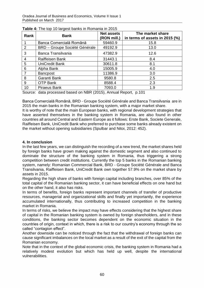
Oradea Journal of Business and Economics, Volume II Issue 1 Published on March 2017
60
Table 4: The top 10 largest banks in Romania in 2015
Rank Bank Net assets (RON mill.)
The market share in terms of assets in 2015 (%)
1 Banca Comercială Română 59460.9 15.8 2 BRD – Groupe Société Générale 49192.9 13.0
3 Banca Transilvania 47382.9 12.6
4 Raiffeisen Bank 31443.1 8.4 5 UniCredit Bank 30611.8 8.1 6 Alpha Bank 15005.9 4.0 7 Bancpost 11386.9 3.0 8 Garanti Bank 9580.8 2.5 9 OTP Bank 8588.4 2.3 10 Piraeus Bank 7093.0 1.9
Source: data processed based on NBR (2015), Annual Report, p.101
Banca Comercială Română, BRD - Groupe Société Générale and Banca Transilvania are in 2015 the main banks in the Romanian banking system, with a major market share. It is worthy of note that the main European banks, with regional development strategies that have asserted themselves in the banking system in Romania, are also found in other countries all around Central and Eastern Europe as it follows: Erste Bank, Societe Generale, Raiffeisen Bank, UniCredit Bank who preferred to purchase some banks already existent on the market without opening subsidiaries (Spulbar and Nitoi, 2012: 452). 4. In conclusion In the last few years, we can distinguish the recording of a new trend, the market shares held by foreign banks have grown making against the domestic segment and also continued to dominate the structure of the banking system in Romania, thus triggering a strong competition between credit institutions. Currently the top 5 banks in the Romanian banking system, namely: Romanian Commercial Bank, BRD - Groupe Société Générale and Banca Transilvania, Raiffeisen Bank, UniCredit Bank own together 57.9% on the market share by assets in 2015. Regarding the high share of banks with foreign capital including branches, over 85% of the total capital of the Romanian banking sector, it can have beneficial effects on one hand but on the other hand, it also has risks. In terms of benefits, foreign banks represent important channels of transfer of productive resources, managerial and organizational skills and finally yet importantly, the experience accumulated internationally, thus contributing to increased competition in the banking market in Romania. In terms of risks, we believe the impact may have effects considering that the highest share of capital in the Romanian banking system is owned by foreign shareholders, and in these conditions, the banking sector becomes dependent on the economic situation in the countries of origin, context in which, there is a risk to our country’s economy through the so called “contagion effect”. Another downside can be noticed through the fact that the withdrawal of foreign banks can cause significant imbalances on the local market as a result of the exit of the capital from the Romanian economy. Note that in the context of the global economic crisis, the banking system in Romania had a relatively modest evolution but which has held up well, despite the international vulnerabilities.
Oradea Journal of Business and Economics, Volume II Issue 1 Published on March 2017
61
References Andries, A., Mehdian, S., Stoica, O. (2013). 'Impact of European Integration on Efficiency and Productivity Growth of Romanian Banks', Engineering Economics, vol. 24, no. 3, pp. 187-197. Balaj, D. (2015). 'A Comparison of Financial Performance of Domestic and Foreign banks in Kosovo by Using DuPont Model', Acta Universitatis Danubius. Œconomica, vol.11, no. 6, pp. 71-86. Ghosh, S. (2016). 'Foreign banks in MENA countries: how important? How relevant?', Journal of Economic and Administrative Sciences, vol. 32, no 1, pp.77 – 98. Kandilov, I. T., Leblebicioğlu, A. and Petkova, N. (2016). 'The impact of banking deregulation on inbound foreign direct investment: Transaction-level evidence from the United States', Journal of International Economics, vol.100, pp. 138-159. Morutan, R. A. and Badulescu, D. (2016). 'State-Owned, Acquisition Or Greenfield Banks In The New Eu Member States. A Post-Crisis Analysis', Oradea Journal of Business and Economics, vol. 1, no. 2, pp. 62-71. Mulyaningsih, T., Daly, A. and Miranti, R. (2015). 'Foreign participation and banking competition: Evidence from the Indonesian banking industry', Journal of Financial Stability, vol. 19, pp. 70-82. Mutinelli, M. and Piscitello, L. (2001). 'Foreign direct investment in the banking sector: the case of Italian banks in the'90s', International Business Review, vol. 10, no. 6, pp. 661-685. National Bank of Romania (2014). Annual Report [online], available from:
http://www.bnr.ro/Regular-publications-2504.aspx. [15.07.2016]. National Bank of Romania (2015). Annual Report [online], available from:
http://www.bnr.ro/Regular-publications-2504.aspx. [15.07.2016]. National Bank of Romania (2015). Financial Stability Report [online], available from:
http://www.bnr.ro/Regular-publications-2504.aspx. [15.07.2016]. Niepmann, F. (2015). 'Banking across borders', Journal of International Economics, vol. 96, no. 2, pp. 244-265. Popovici, A. N. (2013). 'Mergers, Acquisitions and Banking Consolidation in Central and Eastern Europe', CES Working Papers, vol.4, pp. 567-576. Simpasa, A. M. (2013). 'Increased foreign bank presence, privatisation and competition in the Zambian banking sector', Managerial Finance, vol. 39, iss: 8, pp. 787 – 808. Spulbar, C. and Nitoi, M. (2012). Sisteme bancare comparate / Comparative analysis of baking systems, Craiova: Sitech. Van Horen, N. (2007). 'Foreign banking in developing countries; origin matters', Emerging Markets Review, vol. 8, no. 2, pp. 81-105. Weill, L. (2003). 'Banking efficiency in transition economies', Economics of transition, vol. 11, no. 3, pp. 569-592. Zaman, G., Vasile, V. (2006). Transferul tehnologic şi investiţiile–priorităţi ale dezvoltării durabile / Technological transfer and investments - priorities for sustainable development, Bucuresti: Expert-CIDE. Bio-note Vasile Cocriş is currently Vice-Dean and Professor at the Faculty of Economics and Business Administration of the “Alexandru Ioan Cuza” University of Iasi, Romania. He was a visiting professor at the University of Omaha, USA, University of Bologna, Italy, and University Nijmegen, Netherlands and his scientific articles have been published in various national and international journals.

Oradea Journal of Business and Economics, Volume II Issue 1 Published on March 2017
62
Maria-Ramona Sârbu is PhD student in Finance at the Doctoral School of Economics and Business Administration of the “Alexandru Ioan Cuza” University of Iasi, Romania, being supervised by Prof. Dr. Vasile Cocriş. As a PhD student, her research interests are related to international trade, economic growth, regional development and corporate social responsibility.
Oradea Journal of Business and Economics, Volume II Issue 1 Published on March 2017
63
ANALYSIS OF THE TRINOM MIGRATION - FDI - COMPETITIVENESS. CASE STUDY: ROMANIA (2004-2015)
Ana Maria Talmaciu (Banu)1, Laura-Mariana Cismaş
2
1 West University of Timisoara, Romania
2 Department of Economics and Business Modelling, Faculty of Economics and Business
Administration, West University of Timisoara, Timisoara, Romania [email protected] [email protected] Abstract: In the context of a global economy, increasingly competitive, the battle for the competitive advantage has become harsh. The attractiveness of countries which influence
the international migration, generate opposite or complementary effects in the countries of origin and destination. Labor migration among highly qualified people stirred controversy on the impact on the economies of the countries involved in the international transfer of human capital. Labor migration, highly qualified or not, produce a change in the investor’s behavior. They will be interested in investing in countries where the workforce is favoring either qualitatively, either financially, or both.The foreign direct investment fluctuates as the dynamics of migration increases. A country with a large number of highly skilled migrants can lose to foreign investors due to the lack of attractiveness of human capital, and, at the same time, a country with a large number of a trained environmental emigrant may be of interest to investors in search of cheap labor. This paper aims to examine the following hypothesis: to which extent the emigration influence the competitive level (measured by GDP) and the foreign direct investments in the origin country. The results confirm the economic theory, showing a correlation, but not a significative one, for the analized years. Keywords: migration, competitiveness, foreign direct investment, correlation. JEL classification: J21, J61, J31. 1. Introduction The international migration, as a globalization effect, is a process that requires effective management of its effects both positive and negative. The transfer of knowledge and the mobility of production factors led to the development of innovative technologies and to potential growth, as well as to improved living standards of the citizens. In the context of a global economy, increasingly competitive, the battle for the competitive advantage has become harsh. The attractiveness of countries which influence the international migration, generate opposite or complementary effects in countries of origin and the destination. Labor migration among highly qualified people stirred controversy on the impact on the economies of the countries involved in the international transfer of human capital. Most often this phenomenon is called "brain-drain" and usually, it occurs between low-income countries and high-income countries (Bein et al, 2008). Moreover, labor migration, highly qualified or not, produce a change in the investor’s behavior. They will be interested in investing in countries where manpower favoring either qualitatively, either financially or both.The foreign direct investment fluctuates as the dynamics of migration increases. A country with a large number of highly skilled migrants can lose to foreign investors due to the lack of
Corresponding author
Oradea Journal of Business and Economics, Volume II Issue 1 Published on March 2017
64
attractiveness of human capital, and, at the same time, a country with a large number of a trained environmental emigrant may be of interest to investors in search of cheap labor. This phenomenon is specific to Romania too, as a country characterized by low income, nd the proportions it has taken becomes worrisome. The local labor market relaxation caused by massive emigration has not changed for the better the lives of those left behind and influenced their behavior toward immigration. A recent study (Goschin, 20013) demonstrated the Romanian’s teenagers’ intention to leave the country at least temporarily. This paper aims to examine the following hypothesis: to which extent the emigration influence the competitive level (measured by GDP) and the foreign direct investments in the origin country. The first part of the paper consists of a review of the literature who studied
these relationships; we also present the work methodology. In the second part of the paper we use an econometric method to examine the relationship between these variables; finally, the data are interpreted. In the last part of the paper, we comment on the results and propose a number of policy lessons. 2. Literature review The link between migration and competitiveness, seen as economic growth, has been verified by numerous studies and their results are mixed. Some studies follow the idea that migration is negatively correlated with the convergence between regions (Blanchard, Katz, 1992 Dolado, 1993), while other case studies have shown positive effects on growth (Barro, Sala-i-Martin 1992 ). In terms of determining the reasons for the decision to migrate, they remain individual, so related to the personal choice. The purposes of the emigrants (especially those with higher education) refers to: the desire to improve the quality of life, the accumulation of resources, scholarships, (in which case the chances to return to the country drop dramatically), etc (Cismas et al, 2009). Regarding the migration of highly skilled labor, most studies have demonstrated that it has the tendency to migrate to countries or regions where the human capital is better rewarded (Roman et al, 2008). Migration depending on the skill level was tested by Hunt and Muller (2004). They reiterated, based on the realities of Canada and the USA, that highly qualified people are attracted to countries with higher wages. Traditional studies have shown that the labor product average and the average income per capita are negatively influenced by highly qualified labor migration (Bhagwati, Hamada, 1974). The impact on the labor market has not yet been well defined, especially in the source countries. Some papers claim that the positive effects predominate (the chance of returning to the country of origin through the transfer of knowledge), and other studies emphasize the negative consequences of loss of the human capital, and thus innovative potentially (Borjas, Card, 2005). Another point of view was studying the situation in which highly skilled labor migration may lead to the creation of business networks (Kim, Lee, 2016). By the highly skilled workforce influences, returned to their countries of origin, and by the large diasporas from the developed, new technologies and innovation resources are transferred to the source countries (Rauch, Trinidad, 2002; Stark et al., 1997). This process creates a network of highly qualified workforce related to country of origin, and further, raises the possibility of the foreign direct investment contracts between countries of origin and countries of destination. Recent studies have argued that the relatively high rates of highly qualified migrants generate increased volume of foreign direct investment in source economies (Docquier and Lodigiani, 2010). This idea is contrary to Samuelson's theory, who considers the relationship between migration and trade (FDI) is a relationship of substitutability, because trade contributes to factor price equalization and therefore, it lowers the incentives for factor mobility (Kim, Lee,
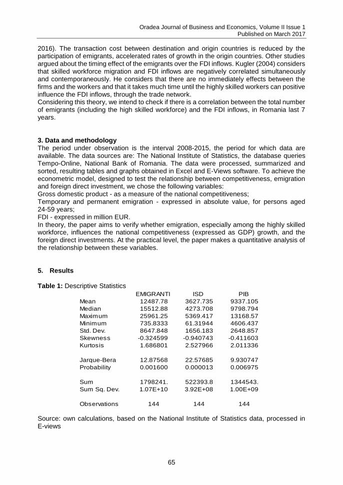
Oradea Journal of Business and Economics, Volume II Issue 1 Published on March 2017
65
2016). The transaction cost between destination and origin countries is reduced by the participation of emigrants, accelerated rates of growth in the origin countries. Other studies argued about the timing effect of the emigrants over the FDI inflows. Kugler (2004) considers that skilled workforce migration and FDI inflows are negatively correlated simultaneously and contemporaneously. He considers that there are no immediately effects between the firms and the workers and that it takes much time until the highly skilled workers can positive influence the FDI inflows, through the trade network. Considering this theory, we intend to check if there is a correlation between the total number of emigrants (including the high skilled workforce) and the FDI inflows, in Romania last 7 years. 3. Data and methodology The period under observation is the interval 2008-2015, the period for which data are available. The data sources are: The National Institute of Statistics, the database queries Tempo-Online, National Bank of Romania. The data were processed, summarized and sorted, resulting tables and graphs obtained in Excel and E-Views software. To achieve the econometric model, designed to test the relationship between competitiveness, emigration and foreign direct investment, we chose the following variables: Gross domestic product - as a measure of the national competitiveness; Temporary and permanent emigration - expressed in absolute value, for persons aged 24-59 years; FDI - expressed in million EUR. In theory, the paper aims to verify whether emigration, especially among the highly skilled workforce, influences the national competitiveness (expressed as GDP) growth, and the foreign direct investments. At the practical level, the paper makes a quantitative analysis of the relationship between these variables. 5. Results Table 1: Descriptive Statistics
EMIGRANTI ISD PIB
Mean 12487.78 3627.735 9337.105
Median 15512.88 4273.708 9798.794
Maximum 25961.25 5369.417 13168.57
Minimum 735.8333 61.31944 4606.437
Std. Dev. 8647.848 1656.183 2648.857
Skewness -0.324599 -0.940743 -0.411603
Kurtosis 1.686801 2.527966 2.011336
Jarque-Bera 12.87568 22.57685 9.930747
Probability 0.001600 0.000013 0.006975
Sum 1798241. 522393.8 1344543.
Sum Sq. Dev. 1.07E+10 3.92E+08 1.00E+09
Observations 144 144 144 Source: own calculations, based on the National Institute of Statistics data, processed in E-views
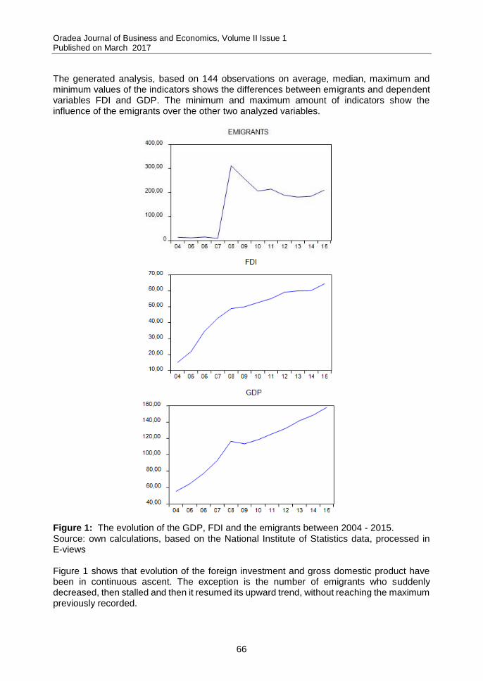
Oradea Journal of Business and Economics, Volume II Issue 1 Published on March 2017
66
The generated analysis, based on 144 observations on average, median, maximum and minimum values of the indicators shows the differences between emigrants and dependent variables FDI and GDP. The minimum and maximum amount of indicators show the influence of the emigrants over the other two analyzed variables.
Figure 1: The evolution of the GDP, FDI and the emigrants between 2004 - 2015. Source: own calculations, based on the National Institute of Statistics data, processed in E-views Figure 1 shows that evolution of the foreign investment and gross domestic product have been in continuous ascent. The exception is the number of emigrants who suddenly decreased, then stalled and then it resumed its upward trend, without reaching the maximum previously recorded.
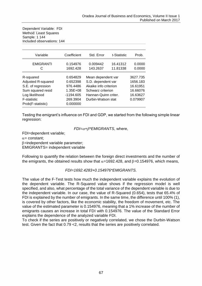
Oradea Journal of Business and Economics, Volume II Issue 1 Published on March 2017
67
Testing the emigrant’s influence on FDI and GDP, we started from the following simple linear regression:
FDI=+*EMIGRANTS, where, FDI=dependent variable;
= constant;
=independent variable parameter; EMIGRANTS= independent variable Following to quantify the relation between the foreign direct investments and the number of
the emigrants, the obtained results show that =1692.428, and =0.154976, which means,
FDI=1692.4283+0.154976*EMIGRANTS.
The value of the F-Test tests how much the independent variable explains the evolution of the dependent variable. The R-Squared value shows if the regression model is well specified, and also, what percentage of the total variance of the dependent variable is due to the independent variable. In our case, the value of R-Squared (0.654), tests that 65.4% of FDI is explained by the number of emigrants. In the same time, the difference until 100% (1), is covered by other factors, like the economic stability, the freedom of movement, etc. The value of the estimated parameter is 0.154976, meaning that a 1% increase of the number of emigrants causes an increase in total FDI with 0.154976. The value of the Standard Error explains the dependence of the analyzed variable FDI. To check if the series are positively or negatively correlated, we chose the Durbin-Watson test. Given the fact that 0.79 <2, results that the series are positively correlated.
Dependent Variable: FDI Method: Least Squares Sample: 1 144 Included observations: 144
Variable Coefficient Std. Error t-Statistic Prob.
EMIGRANTI 0.154976 0.009442 16.41312 0.0000 C 1692.428 143.2637 11.81338 0.0000
R-squared 0.654829 Mean dependent var 3627.735 Adjusted R-squared 0.652398 S.D. dependent var 1656.183 S.E. of regression 976.4486 Akaike info criterion 16.61951 Sum squared resid 1.35E+08 Schwarz criterion 16.66076 Log likelihood -1194.605 Hannan-Quinn criter. 16.63627 F-statistic 269.3904 Durbin-Watson stat 0.079907 Prob(F-statistic) 0.000000
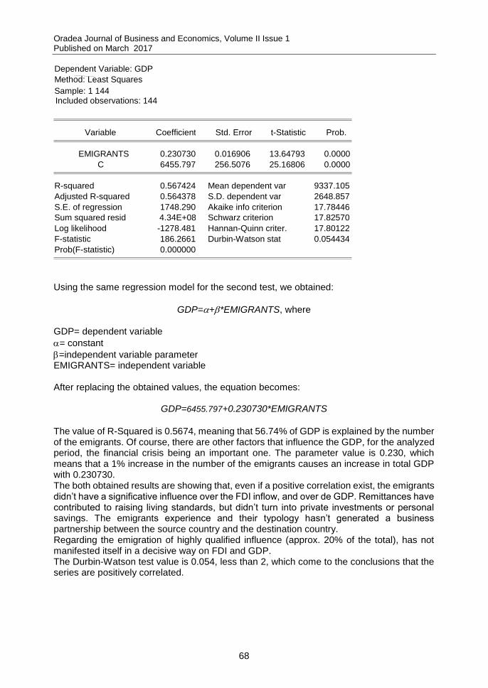
Oradea Journal of Business and Economics, Volume II Issue 1 Published on March 2017
68
Using the same regression model for the second test, we obtained:
GDP=+*EMIGRANTS, where GDP= dependent variable
= constant
=independent variable parameter EMIGRANTS= independent variable After replacing the obtained values, the equation becomes:
GDP=6455.797+0.230730*EMIGRANTS
The value of R-Squared is 0.5674, meaning that 56.74% of GDP is explained by the number of the emigrants. Of course, there are other factors that influence the GDP, for the analyzed period, the financial crisis being an important one. The parameter value is 0.230, which means that a 1% increase in the number of the emigrants causes an increase in total GDP with 0.230730. The both obtained results are showing that, even if a positive correlation exist, the emigrants didn’t have a significative influence over the FDI inflow, and over de GDP. Remittances have contributed to raising living standards, but didn’t turn into private investments or personal savings. The emigrants experience and their typology hasn’t generated a business partnership between the source country and the destination country. Regarding the emigration of highly qualified influence (approx. 20% of the total), has not manifested itself in a decisive way on FDI and GDP. The Durbin-Watson test value is 0.054, less than 2, which come to the conclusions that the series are positively correlated.
Dependent Variable: GDP Method: Least Squares
Sample: 1 144 Included observations: 144
Variable Coefficient Std. Error t-Statistic Prob.
EMIGRANTS 0.230730 0.016906 13.64793 0.0000 C 6455.797 256.5076 25.16806 0.0000
R-squared 0.567424 Mean dependent var 9337.105 Adjusted R-squared 0.564378 S.D. dependent var 2648.857 S.E. of regression 1748.290 Akaike info criterion 17.78446 Sum squared resid 4.34E+08 Schwarz criterion 17.82570 Log likelihood -1278.481 Hannan-Quinn criter. 17.80122 F-statistic 186.2661 Durbin-Watson stat 0.054434 Prob(F-statistic) 0.000000
Oradea Journal of Business and Economics, Volume II Issue 1 Published on March 2017
69
6. Conclusions The effects of the highly skilled migration on the labor market for Romanian and private sector performance is focused on: - the reduced degree of specialization of labor, the departure of highly qualified, unmet wage levels and working conditions; they are prone to remain in the country of destination, determined by the attractiveness of the environment; - lowering the quality of local goods and services by replacing permanent staff caused by the intention to migrate; this leads to increased labor costs and reduce productivity; Romanian private sector warned of the difficulty of recruiting qualified personnel and called on the national authorities to promote the country return; - Weakening the training effect on certain key areas of the Romanian economy, with high potential in the field of IT or research in medicine; reduced budgetary allocations for R&D hinders development areas in which Romania can become competitive and hence the related sectors; The statistical data and the forecasts are showing that, for Romania, human capital is a too "expensive" resource to be "exported" in such a large number. First, is a waste of added value that could be achieved in the country, a loss of economic growth sources in the long term, a lack of economic activities capitalization (with real expression in taxes, profits, salaries, contributions to foreign investment, etc.). Secondly, the lack of capitalization of public spending in education is equivalent to "sponsorship" the destination countries, with a highly qualified workforce at lower costs than the domestic ones. Lastly, the technological advancement and the innovation were weakened by the migratory attitude of the Romanian citizens. In this way the negative effects occur on productivity and national competitiveness, especially by raising employment deficits, depending on the level of education and areas of activity. The positive effects focus on easing the labor market, reducing the unemployment, and reducing the pressure on the state on the allocation of social funds from the public budget. Analyzing the cost-benefit of migratory flux in Romania, we find that, at present, increasing the number of emigrants would lead to weakening the competitive forces of Romania. Therefore we believe that the authorities should consider the following measures: - Promoting fiscal programs for the private sector, encouraging the employment of specialists in competitive wage. In fact, the intention to migrate is influenced by the dynamics and the productivity of the private sector, and local communities are those that can influence it to a large extent; - Initiating effective rewards to induce the emigrants to return home. This would involve implementing strategies to capitalize the human resources potential, guaranteeing higher requirements jobs, involving the best specialists in the local/regional recognition management, facilitating access to the labor market. - Improving the public-private partnership, by encouraging young highly skilled graduates to work in Romania. References Annoni, P., Dijkstra, L. (2013). EU Regional Competitiveness Index RCI 2013. Joint Research Center, Scientific and Policy Reports. European Commision. Arslan, C. et al. (2014). ‘A New Profile of Migrants in the Aftermath of the Recent Economic Crisis’, OECD Social, Employment and Migration Working Papers, no. 160, OECD Publishing. Barro, R., J., Sala-i-Martin-X. (1995). Economic Growth, New York: McGraw-Hill. Bhagwati, J., Hamado, K. (2003). ‘The Brain Drain International Integration of Markets for Professionals and Unemployment: A Theoretical Analysis’, Journal of Development Economics, vol. 1, no. 1, pp. 19-42.
Oradea Journal of Business and Economics, Volume II Issue 1 Published on March 2017
70
Blanchard, O., Kaptz, L. (1992). ‘Regional Evolutions’, Brooking Papers on Economic Activity, 1, pp. 1-61. Borjas, G., J. (2005). ‘The Labor Market Impact of High Skill Immigration’, American Economic Review, vol. 95, no. 2, pp. 56-60. Boshma, R. (2004). ‘Competitiveness of Region from an Evolutionary Perspective’, Regional studies, vol. 38, no. 9, pp.1001-1014. Card, D. (2005), ‘Is The New Immigration Really So Bad?’, Economic Journal, vol. 115, no. 507, pp. 300-323. Cismaş, L., M., Muţiu F., Asproniu, A. (2009). Globalisation, Migration, Mobility and Human Rights: Romanian Perspectives under the Influence of the Global Crisis, Universitatea de Vest din Timişoara. Cismas, L., Sîrghi, N. (2013). Quality Assurance in Education by Linking the Romanian Academic System to Europe 2020 Objectives. Timişoara. Gardiner, Martin, R., Tyler, P. (2004). Competitiveness, Productivity and Economic Growth across the European Regions, University of Cambridge. Kim, J., Lee, N., Y. (2016). ‘The Effect of High Skilled Emigration, Foreign Direct Investment and Policy on the Growth Rate of Source Countries: A Panel Analysis’. East Asian Economic Review, vol. 20, no. 2, pp. 229-275. Kugler, M. and H. Rapoport, (2004) “Skilled Emigration, Business Networks and Foreign
Direct Investment,” CESIFO Area Conference on Global Economy.Munich, available at
http://el.mouhoub.mouhoud.free.fr/wp-content/kuegler-et-rapoport.pdf, [28.01.2017]
Lindsay Lowell B., Findlay A. (2001). Migration Of Highly Skilled Persons From Developing Countries: Impact And Policy Responses Draft Synthesis Report, p.10, available from: https://www.researchgate.net/publication/237112464 [03.02.2017]. Lowell, B. L., Findlay, A. (2007). Migration of highly skilled persons from developing countries: impact and policy responses, International Labour Office Department for International Development, Uk Project Int/01/M09/Ukm: Skilled Labour Migration (The “Brain Drain”) From Developing Countries: Analysis Of Impact And Policy Issues. National Institute of Statistics, Tempo Online Statistics, available from: http://statistici.insse.ro/shop/?lang=ro [17.02.2017] OECD (1996). Trends in international migration, continuous reporting system on migration annual report, OECD. Roman, M., Jaba, E., Goschin, Z., Heanu, B. (2008). Human Capital of Romanian Emigrants in Europe, paper supported by CNCSIS grant IDEI 1829/2008: The Effects of Labor Force Migration and Demographical Structural Changes on the Dynamic of Economics. Stark, O., Helmenstein, C., Prskawetz, A. (1997). ‘A Brain Gain with a Brain Drain’, Economics Letters, vol. 55, no. 2, pp. 227-234. The National Bank of Romania, Foreign direct investment in Romania - annual report, available from: http://www.bnr.ro/PublicationDocuments.aspx?icid=9403 [02.02.2017]. Trinidate, V., Rauch, J., E. (2002). ‘Ethnic Chinese Networks in International Trade’, Review Of Economics And Statistics, vol. 84, no. 1, pp. 116-130. United Nations (2013). World Migration in Figures, A joint contribution by UN-DESA and the OECD to the United Nations High-Level Dialogue on Migration and Development, Department of economic and Social Affairs2013, OECD-UNDESA.
Oradea Journal of Business and Economics, Volume II Issue 1 Published on March 2017
71
Bio-note Ana Maria Talmaciu (Banu) is a Ph.D. candidate at Faculty of Economics and Business Administration, West University of Timisoara, Romania. Her interests include Economy, Competitiveness, Economic Forecast, European Union Economiy, Society. Her thesis is on Romania's competitiveness in relation to the Europe 2020 targets. Until now she presented 4 scientific papers at International Conferences and 1 at National Conferences. Prof. Laura-Mariana Cismaş, PhD., Director of the Economics and Business Modelling Department, West University of Timisoara, Faculty of Economy and Business Administration, Departament of Economy, is specialized in Economy, Microeconomics, Macroeconomics, Political economics, International Economics, European Union Economy, European Social Model Details. She has numerous scientific papers presented and published in prestigious journals along with books and courses.
Oradea Journal of Business and Economics, Volume II Issue 1 Published on March 2017
72
THE PRICE EVOLUTION IN THE CONTEXT OF ECONOMIC CRISIS
Doriana Andreea Rămescu1, Nicoleta Sîrghi
2
1, 2 Department of Economics and Business Modelling, Faculty of Economics and Business
Administration, West University of Timisoara, Timisoara, Romania [email protected] [email protected] Abstract: The economic crisis is a negative macroeconomic phenomenon with consequences both at European Union level and worldwide. The main objective of this paper is to analyse the variation of price levels in Romania, during the economic crisis until the end of 2015, compared with the Member States of the European Union and the countries of the European Free Trade Association. For this research, information provided by EUROSTAT was used, such as price level indices for actual individual consumption per capita, and for different goods and services, calculated based on purchasing power parity. The aim is to identify solutions to rising living standards, compared with more developed countries of the European Union. This paper presents possible solutions for avoiding a future economic crisis, caused by overconsumption. The paper is divided into four sections: introduction, part two which presents aspects of the economic crisis in Romania and in the European Union, the third part presents price level indices for different products and services in 2015, and the last part, the conclusions of the research. Keywords: Economic crisis, Price level, Consumption, Purchasing power parity. JEL classification: E37, E31, E29, C32. 1. Introduction One of the distinctive features of the economic crisis was a sudden collapse of credit on a global level, as banks stopped lending to each other, in fear of unknown and uncertain exposure to toxic debts (Roubini, Mihm, 2010). This effect was also experienced in South East Europe where a sudden stop in credit growth struck almost all the countries at the same time (Bartlett, Prica, 2012).The economic crisis that Romania has gone through was mainly a domestic crisis, caused by the wrong mix of macroeconomic policies taken in the recent years. Economic growth proved to be one of the unhealthy natures, and that's because Romania had in those years an economical growth based on excessive consumption financed by debt. (Donath, Cismaş, 2009). This state of affairs is valid for the government, for companies and for the population. In this paper, we aim to analyse the impact of economic crisis on the economy and price levels for consumer goods and services in Romania and the European Union (EU). We focus on price level indices (PLIs) which offer a comparison of price levels between countries in relation with the EU average, calculated based on purchasing power parity. The price levels for the following consumer goods are analysed: food and non-alcoholic beverages, alcoholic beverages and tobacco, clothing and footwear; and for the following services: water, electricity, gas and other fuels, health and education.
Corresponding author
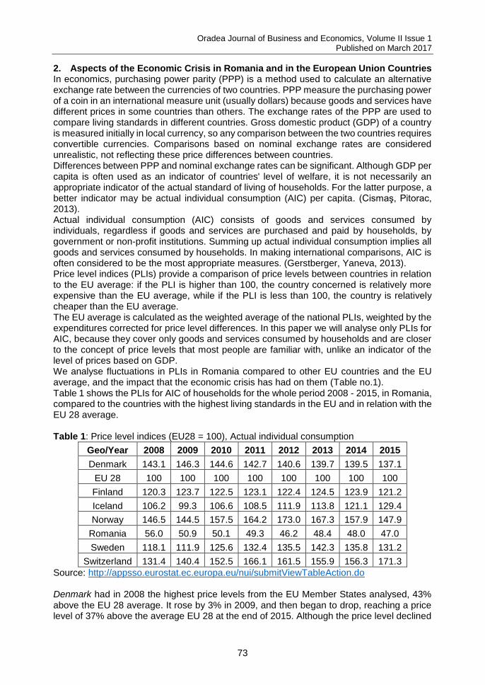
Oradea Journal of Business and Economics, Volume II Issue 1 Published on March 2017
73
2. Aspects of the Economic Crisis in Romania and in the European Union Countries In economics, purchasing power parity (PPP) is a method used to calculate an alternative exchange rate between the currencies of two countries. PPP measure the purchasing power of a coin in an international measure unit (usually dollars) because goods and services have different prices in some countries than others. The exchange rates of the PPP are used to compare living standards in different countries. Gross domestic product (GDP) of a country is measured initially in local currency, so any comparison between the two countries requires convertible currencies. Comparisons based on nominal exchange rates are considered unrealistic, not reflecting these price differences between countries. Differences between PPP and nominal exchange rates can be significant. Although GDP per capita is often used as an indicator of countries' level of welfare, it is not necessarily an appropriate indicator of the actual standard of living of households. For the latter purpose, a better indicator may be actual individual consumption (AIC) per capita. (Cismaş, Pitorac, 2013). Actual individual consumption (AIC) consists of goods and services consumed by individuals, regardless if goods and services are purchased and paid by households, by government or non-profit institutions. Summing up actual individual consumption implies all goods and services consumed by households. In making international comparisons, AIC is often considered to be the most appropriate measures. (Gerstberger, Yaneva, 2013). Price level indices (PLIs) provide a comparison of price levels between countries in relation to the EU average: if the PLI is higher than 100, the country concerned is relatively more expensive than the EU average, while if the PLI is less than 100, the country is relatively cheaper than the EU average. The EU average is calculated as the weighted average of the national PLIs, weighted by the expenditures corrected for price level differences. In this paper we will analyse only PLIs for AIC, because they cover only goods and services consumed by households and are closer to the concept of price levels that most people are familiar with, unlike an indicator of the level of prices based on GDP. We analyse fluctuations in PLIs in Romania compared to other EU countries and the EU average, and the impact that the economic crisis has had on them (Table no.1). Table 1 shows the PLIs for AIC of households for the whole period 2008 - 2015, in Romania, compared to the countries with the highest living standards in the EU and in relation with the EU 28 average. Table 1: Price level indices (EU28 = 100), Actual individual consumption
Geo/Year 2008 2009 2010 2011 2012 2013 2014 2015
Denmark 143.1 146.3 144.6 142.7 140.6 139.7 139.5 137.1
EU 28 100 100 100 100 100 100 100 100
Finland 120.3 123.7 122.5 123.1 122.4 124.5 123.9 121.2
Iceland 106.2 99.3 106.6 108.5 111.9 113.8 121.1 129.4
Norway 146.5 144.5 157.5 164.2 173.0 167.3 157.9 147.9
Romania 56.0 50.9 50.1 49.3 46.2 48.4 48.0 47.0
Sweden 118.1 111.9 125.6 132.4 135.5 142.3 135.8 131.2
Switzerland 131.4 140.4 152.5 166.1 161.5 155.9 156.3 171.3
Source: http://appsso.eurostat.ec.europa.eu/nui/submitViewTableAction.do Denmark had in 2008 the highest price levels from the EU Member States analysed, 43% above the EU 28 average. It rose by 3% in 2009, and then began to drop, reaching a price level of 37% above the average EU 28 at the end of 2015. Although the price level declined
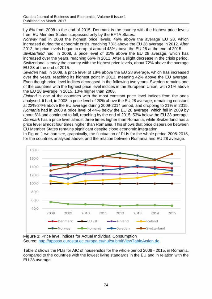
Oradea Journal of Business and Economics, Volume II Issue 1 Published on March 2017
74
by 6% from 2008 to the end of 2015, Denmark is the country with the highest price levels from EU Member States, surpassed only by the EFTA States. Norway had in 2008 the highest price levels, 46% above the average EU 28, which increased during the economic crisis, reaching 73% above the EU 28 average in 2012. After 2012 the price levels began to drop at around 48% above the EU 28 at the end of 2015. Switzerland had, in 2008, a price level of 31% above the EU 28 average, which has increased over the years, reaching 66% in 2011. After a slight decrease in the crisis period, Switzerland is today the country with the highest price levels, about 72% above the average EU 28 at the end of 2015. Sweden had, in 2008, a price level of 18% above the EU 28 average, which has increased over the years, reaching its highest point in 2013, meaning 42% above the EU average. Even though price level indices decreased in the following two years, Sweden remains one of the countries with the highest price level indices in the European Union, with 31% above the EU 28 average in 2015, 13% higher than 2008. Finland is one of the countries with the most constant price level indices from the ones analysed. It had, in 2008, a price level of 20% above the EU 28 average, remaining constant at 22%-24% above the EU average during 2009-2014 period, and dropping to 21% in 2015. Romania had in 2008 a price level of 44% below the EU 28 average, which fell in 2009 by about 6% and continued to fall, reaching by the end of 2015, 53% below the EU 28 average. Denmark has a price level almost three times higher than Romania, while Switzerland has a price level almost four times higher than Romania. This shows that price dispersion between EU Member States remains significant despite close economic integration. In Figure 1 we can see, graphically, the fluctuation of PLIs for the whole period 2008-2015, for the countries analysed above, and the relation between Romania and EU 28 average.
Figure 1: Price level indices for Actual Individual Consumption Source: http://appsso.eurostat.ec.europa.eu/nui/submitViewTableAction.do Table 2 shows the PLIs for AIC of households for the whole period 2008 - 2015, in Romania, compared to the countries with the lowest living standards in the EU and in relation with the EU 28 average.
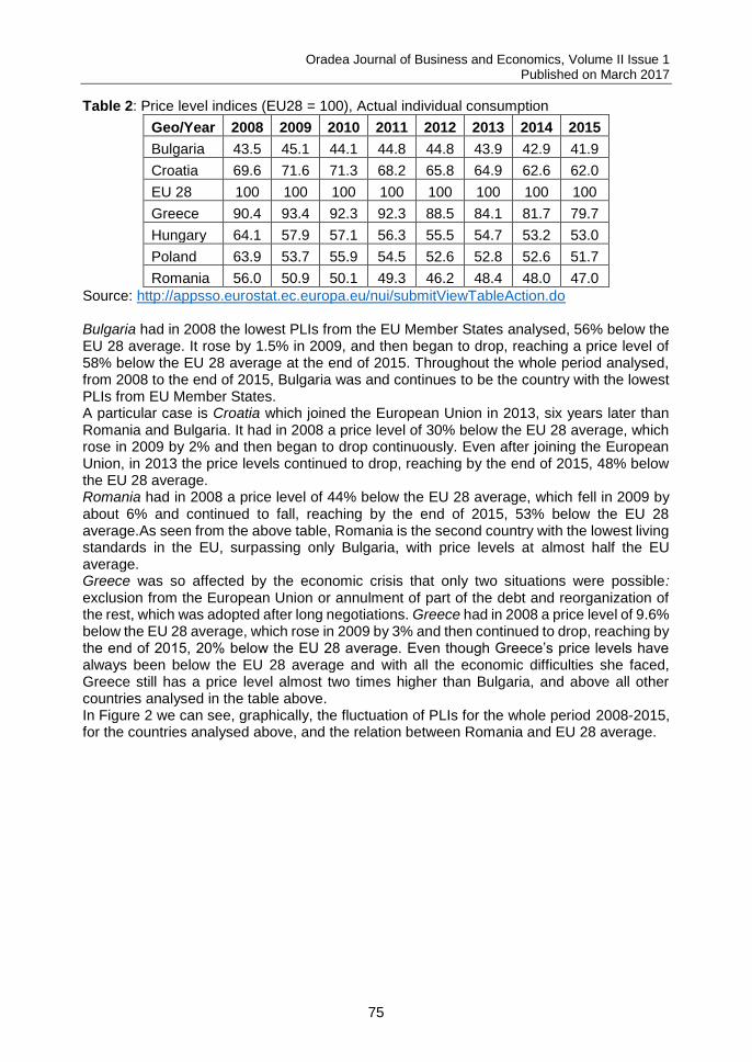
Oradea Journal of Business and Economics, Volume II Issue 1 Published on March 2017
75
Table 2: Price level indices (EU28 = 100), Actual individual consumption
Geo/Year 2008 2009 2010 2011 2012 2013 2014 2015
Bulgaria 43.5 45.1 44.1 44.8 44.8 43.9 42.9 41.9
Croatia 69.6 71.6 71.3 68.2 65.8 64.9 62.6 62.0
EU 28 100 100 100 100 100 100 100 100
Greece 90.4 93.4 92.3 92.3 88.5 84.1 81.7 79.7
Hungary 64.1 57.9 57.1 56.3 55.5 54.7 53.2 53.0
Poland 63.9 53.7 55.9 54.5 52.6 52.8 52.6 51.7
Romania 56.0 50.9 50.1 49.3 46.2 48.4 48.0 47.0
Source: http://appsso.eurostat.ec.europa.eu/nui/submitViewTableAction.do Bulgaria had in 2008 the lowest PLIs from the EU Member States analysed, 56% below the EU 28 average. It rose by 1.5% in 2009, and then began to drop, reaching a price level of 58% below the EU 28 average at the end of 2015. Throughout the whole period analysed, from 2008 to the end of 2015, Bulgaria was and continues to be the country with the lowest PLIs from EU Member States. A particular case is Croatia which joined the European Union in 2013, six years later than Romania and Bulgaria. It had in 2008 a price level of 30% below the EU 28 average, which rose in 2009 by 2% and then began to drop continuously. Even after joining the European Union, in 2013 the price levels continued to drop, reaching by the end of 2015, 48% below the EU 28 average. Romania had in 2008 a price level of 44% below the EU 28 average, which fell in 2009 by about 6% and continued to fall, reaching by the end of 2015, 53% below the EU 28 average.As seen from the above table, Romania is the second country with the lowest living standards in the EU, surpassing only Bulgaria, with price levels at almost half the EU average. Greece was so affected by the economic crisis that only two situations were possible: exclusion from the European Union or annulment of part of the debt and reorganization of the rest, which was adopted after long negotiations. Greece had in 2008 a price level of 9.6% below the EU 28 average, which rose in 2009 by 3% and then continued to drop, reaching by the end of 2015, 20% below the EU 28 average. Even though Greece’s price levels have always been below the EU 28 average and with all the economic difficulties she faced, Greece still has a price level almost two times higher than Bulgaria, and above all other countries analysed in the table above. In Figure 2 we can see, graphically, the fluctuation of PLIs for the whole period 2008-2015, for the countries analysed above, and the relation between Romania and EU 28 average.
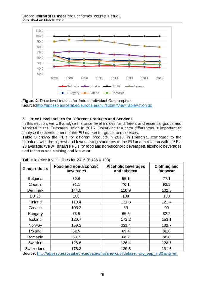
Oradea Journal of Business and Economics, Volume II Issue 1 Published on March 2017
76
Figure 2: Price level indices for Actual Individual Consumption Source:http://appsso.eurostat.ec.europa.eu/nui/submitViewTableAction.do 3. Price Level Indices for Different Products and Services In this section, we will analyse the price level indices for different and essential goods and services in the European Union in 2015. Observing the price differences is important to analyse the development of the EU market for goods and services. Table 3 shows the PLIs for different products in 2015, in Romania, compared to the countries with the highest and lowest living standards in the EU and in relation with the EU 28 average. We will analyse PLIs for food and non-alcoholic beverages, alcoholic beverages and tobacco and clothing and footwear. Table 3: Price level indices for 2015 (EU28 = 100)
Geo/products Food and non-alcoholic
beverages Alcoholic beverages
and tobacco Clothing and
footwear
Bulgaria 69.6 55.1 77.1
Croatia 91.1 70.1 93.3
Denmark 144.6 118.9 132.6
EU 28 100 100 100
Finland 119.4 131.8 121.4
Greece 103.2 89 99
Hungary 78.9 65.3 83.2
Iceland 129.7 173.2 153.1
Norway 159.2 221.4 132.7
Poland 62.5 69.4 92.6
Romania 63.7 68.7 88.8
Sweden 123.6 126.4 128.7
Switzerland 173.2 129.3 131.3
Source: http://appsso.eurostat.ec.europa.eu/nui/show.do?dataset=prc_ppp_ind&lang=en
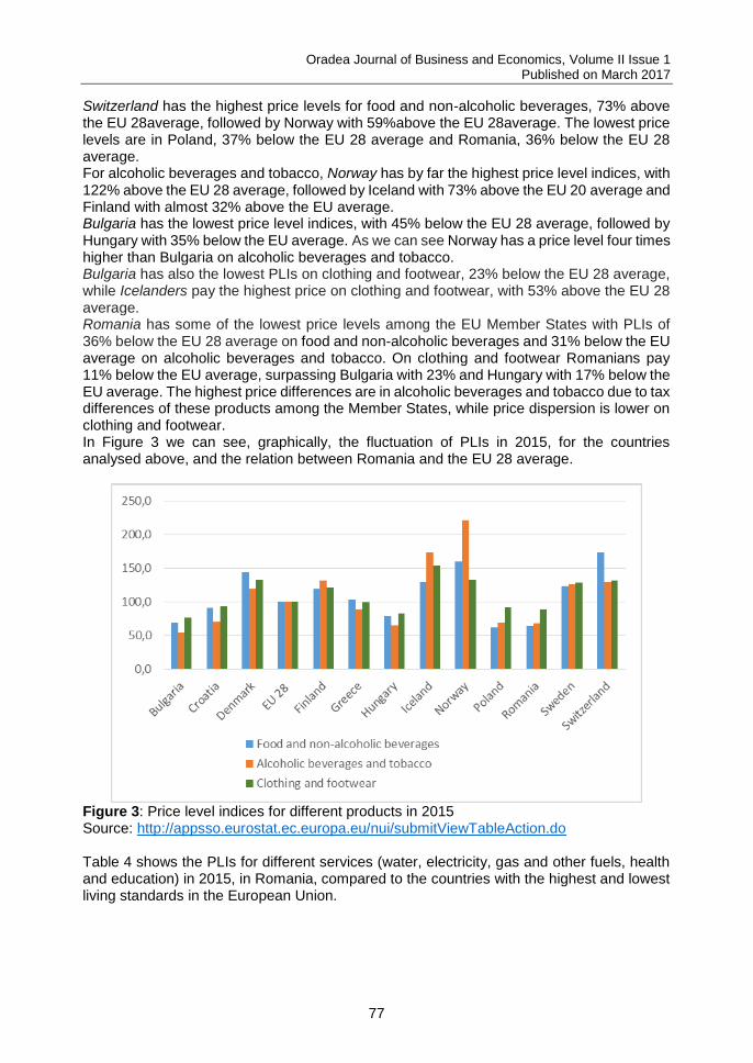
Oradea Journal of Business and Economics, Volume II Issue 1 Published on March 2017
77
Switzerland has the highest price levels for food and non-alcoholic beverages, 73% above the EU 28average, followed by Norway with 59%above the EU 28average. The lowest price levels are in Poland, 37% below the EU 28 average and Romania, 36% below the EU 28 average. For alcoholic beverages and tobacco, Norway has by far the highest price level indices, with 122% above the EU 28 average, followed by Iceland with 73% above the EU 20 average and Finland with almost 32% above the EU average. Bulgaria has the lowest price level indices, with 45% below the EU 28 average, followed by Hungary with 35% below the EU average. As we can see Norway has a price level four times higher than Bulgaria on alcoholic beverages and tobacco. Bulgaria has also the lowest PLIs on clothing and footwear, 23% below the EU 28 average, while Icelanders pay the highest price on clothing and footwear, with 53% above the EU 28 average. Romania has some of the lowest price levels among the EU Member States with PLIs of 36% below the EU 28 average on food and non-alcoholic beverages and 31% below the EU average on alcoholic beverages and tobacco. On clothing and footwear Romanians pay 11% below the EU average, surpassing Bulgaria with 23% and Hungary with 17% below the EU average. The highest price differences are in alcoholic beverages and tobacco due to tax differences of these products among the Member States, while price dispersion is lower on clothing and footwear. In Figure 3 we can see, graphically, the fluctuation of PLIs in 2015, for the countries analysed above, and the relation between Romania and the EU 28 average.
Figure 3: Price level indices for different products in 2015 Source: http://appsso.eurostat.ec.europa.eu/nui/submitViewTableAction.do Table 4 shows the PLIs for different services (water, electricity, gas and other fuels, health and education) in 2015, in Romania, compared to the countries with the highest and lowest living standards in the European Union.
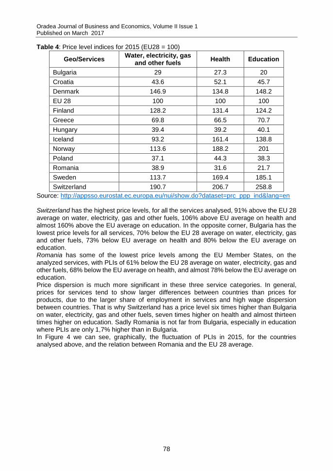
Oradea Journal of Business and Economics, Volume II Issue 1 Published on March 2017
78
Table 4: Price level indices for 2015 (EU28 = 100)
Geo/Services Water, electricity, gas
and other fuels Health Education
Bulgaria 29 27.3 20
Croatia 43.6 52.1 45.7
Denmark 146.9 134.8 148.2
EU 28 100 100 100
Finland 128.2 131.4 124.2
Greece 69.8 66.5 70.7
Hungary 39.4 39.2 40.1
Iceland 93.2 161.4 138.8
Norway 113.6 188.2 201
Poland 37.1 44.3 38.3
Romania 38.9 31.6 21.7
Sweden 113.7 169.4 185.1
Switzerland 190.7 206.7 258.8
Source: http://appsso.eurostat.ec.europa.eu/nui/show.do?dataset=prc_ppp_ind&lang=en Switzerland has the highest price levels, for all the services analysed, 91% above the EU 28 average on water, electricity, gas and other fuels, 106% above EU average on health and almost 160% above the EU average on education. In the opposite corner, Bulgaria has the lowest price levels for all services, 70% below the EU 28 average on water, electricity, gas and other fuels, 73% below EU average on health and 80% below the EU average on education. Romania has some of the lowest price levels among the EU Member States, on the analyzed services, with PLIs of 61% below the EU 28 average on water, electricity, gas and other fuels, 68% below the EU average on health, and almost 78% below the EU average on education. Price dispersion is much more significant in these three service categories. In general, prices for services tend to show larger differences between countries than prices for products, due to the larger share of employment in services and high wage dispersion between countries. That is why Switzerland has a price level six times higher than Bulgaria on water, electricity, gas and other fuels, seven times higher on health and almost thirteen times higher on education. Sadly Romania is not far from Bulgaria, especially in education where PLIs are only 1,7% higher than in Bulgaria. In Figure 4 we can see, graphically, the fluctuation of PLIs in 2015, for the countries analysed above, and the relation between Romania and the EU 28 average.
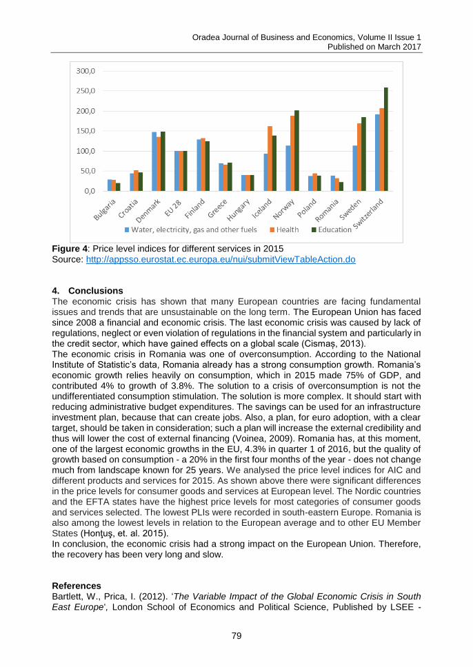
Oradea Journal of Business and Economics, Volume II Issue 1 Published on March 2017
79
Figure 4: Price level indices for different services in 2015 Source: http://appsso.eurostat.ec.europa.eu/nui/submitViewTableAction.do 4. Conclusions The economic crisis has shown that many European countries are facing fundamental issues and trends that are unsustainable on the long term. The European Union has faced since 2008 a financial and economic crisis. The last economic crisis was caused by lack of regulations, neglect or even violation of regulations in the financial system and particularly in the credit sector, which have gained effects on a global scale (Cismaș, 2013). The economic crisis in Romania was one of overconsumption. According to the National Institute of Statistic’s data, Romania already has a strong consumption growth. Romania’s economic growth relies heavily on consumption, which in 2015 made 75% of GDP, and contributed 4% to growth of 3.8%. The solution to a crisis of overconsumption is not the undifferentiated consumption stimulation. The solution is more complex. It should start with reducing administrative budget expenditures. The savings can be used for an infrastructure investment plan, because that can create jobs. Also, a plan, for euro adoption, with a clear target, should be taken in consideration; such a plan will increase the external credibility and thus will lower the cost of external financing (Voinea, 2009). Romania has, at this moment, one of the largest economic growths in the EU, 4.3% in quarter 1 of 2016, but the quality of growth based on consumption - a 20% in the first four months of the year - does not change much from landscape known for 25 years. We analysed the price level indices for AIC and different products and services for 2015. As shown above there were significant differences in the price levels for consumer goods and services at European level. The Nordic countries and the EFTA states have the highest price levels for most categories of consumer goods and services selected. The lowest PLIs were recorded in south-eastern Europe. Romania is also among the lowest levels in relation to the European average and to other EU Member States (Honţuş, et. al. 2015). In conclusion, the economic crisis had a strong impact on the European Union. Therefore, the recovery has been very long and slow. References Bartlett, W., Prica, I. (2012). ‘The Variable Impact of the Global Economic Crisis in South East Europe‘, London School of Economics and Political Science, Published by LSEE -
Oradea Journal of Business and Economics, Volume II Issue 1 Published on March 2017
80
Research on South Eastern Europe, [Online], Available from: http://www.lse.ac.uk/europeanInstitute/research/LSEE/PDFs/Publications/LSEE-PAPER-4.pdf. [30.10.2016]; Cismaş, L., Pitorac, R. (2013). ‘A new vision on competitiveness within the post-crisis economy. Causes, evolutions and possible innovative solutions to fight against the undesirable effects of the economic crisis’, Theoretical and Applied Economics, Vol.XX, no. 10(587), pp. 23-32; Donath, L., Cismaş, L. (2009). ‘The current financial crisis revisited. Causes and remedies’, The Romanian Economic Journal, Year XII, no. 31; Gerstberger, C., Yaneva, D. (2013). ‘Statistics in focus 2/2013 – Eurostat‘, Economy and Finance, [Online], Available from: http://ec.europa.eu/eurostat/documents/3433488/5585636/KS-SF-13-002-EN.PDF/a4a1ed61-bac7-4361-a3f0-4252140e1751?version=1.0. [30.10.2016]; Honţuş, A. C., Mărcuţă, A., Tindeche, C., Mărcuţă, L. (2015). ‘Impact Of The Economic Crisis On European Union During 2008 – 2015 Period’, Scientific Papers Series Management, Economic Engineering in Agriculture and Rural Development vol. 15, [Online], Available from: http://managementjournal.usamv.ro/pdf/vol.15_4/Art17.pdf. [02.02.2017] Roubini, N., Mihm, S. (2010). Crisis Economics, A crash course in the future of finance, The Penguin Press, New York; Voinea, L. (2009). Sfârșitul economiei iluziei, Criză și anticriză. O abordare heterodoxă, Bucuresti: Editura Publica, Ediția 1. Bio-note Doriana Andreea Rămescu is PhD Student, first year of study, at the Faculty of Economics and Business Administration, West University of Timişoara, Romania, and currently she is working on PhD thesis: „Relation competition - game theory in market structures”. Nicoleta Sîrghi, PhD is Professor PhD habil. of Economics at the Faculty of Economics and Business Administration, West University of Timisoara, Romania. Her current research focuses on applied economics, game theory with applications in economics. She has presented a great number of papers in these fields in scientific journals and conference proceedings (IBIMA International Conference, WSEAS International Conference etc.). She has been a regular referee of papers for International Business Information Management Conference (IBIMA). She has published in the International Journal of Bifurcation and Chaos (IJBC), in the Transformations in Business and Economics (TIBE).
Oradea Journal of Business and Economics, Volume II Issue 1 Published on March 2017
81
THE DIFFERENCES BETWEEN WOMEN EXECUTIVES IN JAPAN AND ROMANIA
Irina Roibu1, Paula Alexandra Roibu (Crucianu)
2
1Hankuk University of Foreign Studies, Department of Romanian Studies, Seoul, South
Korea 2Doctoral School of Economics and Business Administration, “Alexandru Ioan Cuza”
University, Iasi, Romania [email protected] [email protected] Abstract: Around the world employment of women on an equal bases allows companies, industries and countries to make better use of the available talent pool, generally with potential growth implication. In Japan, since 2013, Prime Minister Shinzo Abe has been a ceaseless advocate for the increase in the number of female employees for the revival of the economy, and many governmental programs in support of working women have been put in place. However, the traditional Japanese management systems of lifetime employment, enterprise unions, seniority systems, together with a group-oriented and risk-adverse orientation make things change slowly. In Romania, the second country analyzed in this article, women entrepreneurs also face professional stereotypes, difficulties in getting specific jobs, traditional prejudices and a collective mentality related to women’s place in society. This article explores and compares how Romanian and Japanese cultures, societies, and economies have either encouraged, or discouraged, the growth of female entrepreneurship on their own territories, and analyzes how the best emerging female executives can be supported in the future in order to maximize their potential. The analysis is based on the data provided by OECD, the World Bank, the Global entrepreneurship monitor, Japan statistics, the legislations of the two countries and the literature related to the two social environments. The findings indicate that although there are many similarities between the two countries, the percentage of female executives in Japan is much smaller than the one in Romania. This is due to the fact that Japan, with all the governmental programs in action, for the moment, still has a stricter social and work environment, a weaker maternity and childcare legislation and a higher gender gap. Keywords: women executives, Japan, Romania, Japanese business culture, Romanian business culture. JEL classification: B54, F43, R28. 1. Introduction Worldwide, the companies with more women in senior executive positions report stronger financial performance, better reputation and brand advantages. However, the number of female CEOs remains very small: on a global perspective, women make up only 5% of Fortune 500 CEO’s and only 4% of FTSE companies (Weber Shandwick, 2015). This issue is generally the effect of the cultural and organizational issues that prewmoving through the corporate pipeline. Also depending on the geographical area, the society, the culture, etc., the barriers that women executives face can be stronger or weaker, allowing them more or less access to high-level jobs.
Corresponding author
Oradea Journal of Business and Economics, Volume II Issue 1 Published on March 2017
82
As far as Japan and Romania are concerned, in the first chapter we chose to explore how the Japanese mentality, culture, politics and economics affected women entrepreneurship and the number of female executives, as well as the barriers that they have faced etc. The second chapter analyses the same aspects in Romania, while the third chapter makes a comparison between the two countries and suggests ideas on how the situation of female executives can be improved and how they can be supported to maximize their potential. The hypothesis that guided the analysis is that, despite the different historical, economic and cultural backgrounds, the situation of female executives in both countries is very similar. The reasons for choosing these two countries begin with the interest of the authors in the topic of female entrepreneurship, one for the Romanian side and the other for the Japanese one, their location (one in Romania and the other in East Asia) and the worldwide enthusiasm in topics related to Japan. The purpose of the paper is to show what are the development probabilities of executives women in the two countries, based on the premises that the two are located at different development levels and in both women have generally less chances for promotion than men have. 2. Women executives in Japan Traditionally, a Japanese woman’s work life was short: only until her marriage. If she continued working afterwards, it was considered a big loss of face to her husband. Due to this cultural expectation, employers would not “train female employees for jobs beyond making tea or greeting customers” (Subhash and Norton, 1993). At the same time, women were and, in many cases, are still considered as only part-timers and had/have jobs of auxiliary nature, with no supervisory capability (Subhash and Norton, 1993), smaller salaries and lesser opportunities for advancement. Moreover, because the Japanese companies use seniority (that discriminates the short-term employees) and life-time employment systems, women do not have many chances of becoming equal to men at work and gaining promotions to managerial positions. Last but not least, women are excluded from in-company rotation and training programs that are necessary in order to advance. The training received is a minimal one, only related to the way of greeting customers, how to bow, how to use the polite language and perform reception activities, such as answering the phone. One of the reasons for this is the fact that the training is expensive for the company and the costs can be balanced only after a new employee has gained several years of experience. Therefore, in the case of women, where the chance of quitting is high, it would be considered a loss for the company (Subhash and Norton, 1993). However, as anywhere else in the world, in Japan too, the role and status of women has been continuously changing based on economic, cultural and historic conditions. For example, if after the Second World War, Japanese women were needed in the workplace and a high number of them were employed, in the 1960’s, when the country became prosperous, women were sent back home by their husbands in order to look good in terms of social status (Cook and Hayashi, 1980) and as a sign of the family’s affluence. From the 1980s however, women began going back to work again and becoming approximately 50%
of the labor force in 1990 (Labor force participation rate, female; The World Bank). However, in the post bubble economy, they were laid off again, women being the first to lose their jobs in harsh economic situations. At school, girls are “pushed” to choose the major that is more feminine, such as arts, and boys to choose the one that is more masculine, such as science. In universities, the trend of choosing the “appropriate” major based on the student’s gender seems to continue. Women tend to study secretarial skills, English, international relations, psychology, literature and economics (Dirk, 2016) which gives them less chances of finding a good job with access to advancement in a company after graduation. The women who are granted access here are of a high status given by a high position in the company, government, etc. Nevertheless,
Oradea Journal of Business and Economics, Volume II Issue 1 Published on March 2017
83
(Hidaka, 2010), Japanese women are still perceived as inferior due to the fact that they don’t hold jobs of the same status as men do. However, some companies accepted women to hold managerial positions, but in divisions especially created for women. Also, the women who are in managerial positions are generally employed in medium and small size firms, not in large Japanese corporations. An analysis made in 1999 indicated that “most women managers work in their own family-run businesses (33%), or are employed by foreign firms (67%)” (Aggarwal, ed., 1999). Also, as previously mentioned, the most common types of companies run by women continue to be in fields such as clothing, real estate agencies, beauty industry, etc. The number of female presidents in the beauty sector amounted to 35.1% in 2014, 34.4 % in the cosmetic retail business and 29.9% of the total in the senior health care field (Kameda, 2014). It is important to mention that Japanese women are not held back only by patriarchy. Many women from wealthy places like Tokyo prefer to stay at home and enjoy the sansoku hirune tsuki (three meals and a nap) life style, instead of the stressful salaryman one (Japanese women and work. Holding back the half the nation, 2014). Mariko Brando, the author of the book “The dignity of a woman” (2006) points out that many women who are married with high-ranking executives of big companies prefer to have a part time job in a small company or even a supermarket, considering that they don’t need a high-status job to enjoy a high status (Ibid.). Among other reasons emphasized during the present research, the most important are: the lack of a system that ensures an easier access to loans for women, some banks being hesitant of lending money to women due to their gender (Kameda, 2014); lack of mentors and fright to start a business; intimidation by the majority of people’s choices; fear of maternity harassment (women are forced to retire when they become pregnant or give birth) or matahara in Japanese - in a survey conducted in 2014, 26.3 % of women reported experiencing matahara and 27.3 % said they know somebody who has experienced it (Ryan, 2015); the Japanese concepts of harmony preservation and conflict avoidance, which make many women give up instead of fighting for their rights; long working hours; nominication (nomu = to drink and communication) – which is an essential part of maintaining interpersonal relationships with the colleagues, customers, etc. and usually takes place after work, until late at night; short vacations, etc. For married women and working mothers these last mentioned obstacles are very difficult to surpass, due to the housework that also needs to be done by them and the time and attention their family needs. However, in the last years (more specifically since 2013), Abe Government has been encouraging more women to enter the workforce and has created hundreds of thousands of new jobs under Abenomics, even though many of these are part time. However, the rising demands of working women, do not come with better opportunities and work conditions provided by the Japanese corporations. In order for real changes to take place, the society has to be shaken to the core. Or at least, the companies that fail to meet the governmental requirements of the newly created environments should be punished. Nevertheless, the government has set a target of “30% female leadership representation in various fields of Japanese society” by 2020, when Tokyo will host the Olympics (Japan: Women in the workplace, 2015). Be that as it may, the numbers are ambitious, especially in a country where female representation in the parliament’s lower house was 8 % in 2013 and the female manager ratio was 10 % in 2013. Also, Japan is well known for a slow promotion pace, the age limit for getting promoted tending to be higher, especially in case of women (Ishizuka, 2014). Nevertheless, the Japanese Government has taken a step forward in including more women in the economic field and in creating more gender diversity at the management level, in order to fix the mounting fiscal deficits and the population problems (Ishizuka, 2014).
Oradea Journal of Business and Economics, Volume II Issue 1 Published on March 2017
84
3. Women executives in Romania Romania is a former communist country, still struggling with a deeply corrupted environment (Transparency International Romania, 2015). The long years spent under communist control reduced the female entrepreneurial capacities and in many cases, successful models for the young generations are missing. However, by becoming a member of NATO since 2004 and of EU since 2007, new challenges have arisen and the country had to learn how to activate and compete with its European counterparts. Also, by beginning to have access to structural funds from the EU, a financial support platform was created for opening new businesses and improve their skills (Piti, 2015). In time, women started to get more involved in different fields and have access to higher-level jobs. However, an analysis made by the European Commission in 2014 indicated that in Romania men receive a monthly payment with 9.7% better than women, with only 9% of the companies’ board members and 11% of the CEO’s being women. Moreover, Romania ranks 27 by the number of women in the Parliament (11.5%), as shown in the research performed by The Permanent Electoral Authority in 2013. Why these low numbers? As in many other countries, women executives from Romania are equally qualified and have similar competences with men, but at the decision level, the relations are discriminative and asymmetrical. The legislation that supports equality between sexes exists and is observing the strict standards of the European Union. However, in reality, it is just a “law for display”. The gender wage gap still exists (10% in 2014, OECD) and in some cases women receive a job just because the legislation requires that a certain type of company, political party, etc. should include a certain number of men and women. During communism, the party and the state supported women getting involved in the public sphere, breaking the economic barriers imposed by the old traditions and leaving the children in the care of public organizations, naming them “equal socialist workers” and “mothers of the nation” (Massino, 2014). There are two distinct phases during the communist regime regarding the status of women: 1. policies for empowerments at the beginning of communism (1948-1965) and 2. aggressive pro-natalist policies (decree after anti-abortion 1966-1989). The first phase represents the period when in Romania there was an acute need of women labor, thus generating an intense propaganda of emancipation and freedom for women through work (Padurariu, 2014) and second period (“Golden Age”) was characterized by a strict pro-natalist policy. After the fall of communism, many laws related to equality of chances had been adopted. Concerning the maternity leave, the 2005 law (updated several times until 2015) consists of: 63 days of pregnancy leave before birth and 63 days of maternity leave after birth. The monthly child allowance represents 85% of the net average income earned in the last 12 months. There is also a parental leave that both mothers and fathers can take: up to 2 years, with an allowance of 85% from the average net income earned in the last 12 months, maximum 1.200 lei / month (around 300 $) (European Commission). One of the most important aspects for a working woman is the law preventing the employer from firing a pregnant person or who is currently on maternity leave / parental leave. The company has to receive the person back on her/his previous position after the leave is finished. Statistics indicate that 95% of the persons who take parental leave resume their work at the end of it (Marinescu, 2016). This support is extremely important for women who want to combine career with motherhood. Regarding the Romanian career women, their profile is as follows: ambitious, married, with children, average age 36 years, university graduate, devoted to business, working 60 hours/week, independent. The main motivations for Romanian women to open a business are as follows: to be their own boss, personal desire to start a business, opportunity to increase the quality of life, money, contribution to society, etc. (Ramadani, Gërguri-Rashiti, Fayolle, 2015). Their strong points are social networking, intuition, patience, more
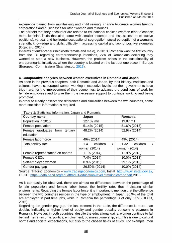
Oradea Journal of Business and Economics, Volume II Issue 1 Published on March 2017
85
experience gained from multitasking and child rearing, chance to create women friendly corporations and businesses for other women and minorities. The barriers that they encounter are related to educational choices (women tend to choose more feminine fields that also come with smaller incomes and less access to executive positions), vertical and horizontal occupational segregation, social perception of a woman’s strength, knowledge and skills, difficulty in accessing capital and lack of positive examples (Cojocaru, 2014). In terms of entrepreneurship (both female and male), in 2013, Romania was the first country from the EU regarding entrepreneurship intentions, 27% of Romanians declaring they wanted to start a new business. However, the problem arises in the sustainability of entrepreneurial initiatives, where the country is located on the last but one place in Europe (European Commission) (Scarlatescu, 2013). 4. Comparative analyses between women executives in Romania and Japan As seen in the previous chapters, both Romania and Japan, by their history, traditions and cultures, have discouraged women working in executive levels, but their governments have tried hard, for the improvement of their economies, to advance the conditions of work for female employees and to give them the necessary support to continue working and being promoted. In order to clearly observe the differences and similarities between the two countries, some more statistical information is required.
Table 1: Statistical information: Japan and Romania
Country name Japan Romania
Population in 2015 127.02 mil 19.87 mil
Female population 51.4% (2015) 51.6% (2015)
Female graduates from tertiary
education
48.2% (2014) 52.9% (2014)
Female labor force 49% (2014) 49% (2014)
Total fertility rate 1.4 children /
woman (2014)
1.32 children /
woman (2014)
Female representation on boards 1.1% (2014) 11.9% (2013)
Female CEOs 7.4% (2014) 10.0% (2013)
Self-employed women 0.9% (2015) 29.1% (2013)
Gender pay gap 26.59% (2014) 10.0% (2014)
Source: Trading Economics – www.tradingeconomics.com, Instat http://www.instat.gov.al/, OECD https://data.oecd.org/eduatt/adult-education-level.htm#indicator-chart,2015 As it can easily be observed, there are almost no differences between the percentage of female population and female labor force, the fertility rate, thus indicating similar environments. Regarding the female labor force, it is important to mention that the difference between the two countries resides in the type of employment: in Japan, 36.9% of the total are employed in part time jobs, while in Romania the percentage is of only 5.5% (OECD, 2015). Regarding the gender pay gap, the last element in the table, the difference is more than double, indicating a higher level of equity and gender equality concerning payment in Romania. However, in both countries, despite the educational gains, women continue to fall behind men in income, politics, employment, business ownership, etc. This is due to cultural norms and societal expectations, but also to the chosen fields of study. For example, men
Oradea Journal of Business and Economics, Volume II Issue 1 Published on March 2017
86
dominate majors such as engineering, computer sciences, manufacturing, while women focus on education, humanities and arts, health and welfare, fields that are less remunerative. Moreover, analyzing the percentages of male and female employed persons by occupation, Japan Statistics 2014 indicated that men are more prominent in construction and mining (98.4%), transport and machine operation (97.3%), while women were prominent among medical, health services (75.3%), clerical work (59.7%) and accommodation, eating and drinking services (62.1%). In Romania, women are prominent in health and social assistance (59%), private household (67%), other services (52%), education (49%), hotels and restaurants (42.6%) (Popescu, 2016). Compared to their Romanian counterparts, Japanese women are the managers of the family and the house, they assume total responsibility for the family, giving freedom to the husband to only be in charge of the economic production and no other aspects (Renshaw, 1999, p. 28). On the other side, Romanian women share with their husbands both the economic production and the house management, giving more time to women for other activities. The present social trends in Japan present a new type of men and women, called herbivore men and carnivore women. Carnivore women refer to women that are active and more internationally minded, while men are taking low-responsibility jobs and do not want to get married, living in the old model breadwinner / housewife style (Japanese women and work. Holding back the half the nation, 2014). Japanese women, as the author Lefcadio Hearn said, are the most wonderful aesthetic products of Japan. They are seen by foreigners and Japanese men as “precious possessions, pleasing to behold, docile and manageable” (Renshaw, 1999, p. 16). Also, the term Ryosaikenbo, which means good wife, wise mother, introduces the traditional idea of a woman as house organizer, child and husband caretaker. Another expression, onna ha sanpo sagatte, meaning that a woman should walk 3 steps behind her husband, represents the traditional view of how a couple should behave in public and what is the place of each of them in the society: man first, woman second. Moreover, the Confucian belief supported the supremacy of men and said “As a samurai, be with a woman in public itself is bad”, indicating again the place of a woman far from the man. All these theories indicate that a woman’s place is not near a man, in the public space at least, the same mentality being applied to the work environment. This adds to the idea of the filmmaker Juno Itami, who declared that a Japanese woman is supposed to renounce men and family in order to succeed “on the rough road to corporate success” (Renshaw, 1999), indicating the society’s inflexibility towards women working. Moreover, in a country like Japan, where the people’s opinion has a big influence upon others, if the attitudes toward women working are negative, most often they will give up trying, the biggest challenge for female executives in Japan being to reluct against this socio-cultural aspect. 5. Support for female executives to maximize their potential As previously mentioned, in the last years the Japanese Government tried to encourage women with business and career aspirations through a series of adopted policies. The press has been naming the prime minister’s approach as “Womenomics” (increased participation of women in the economy), and is considered a pillar for the prime minister’s campaign for economic revitalization. However, as the 2015 Female Entrepreneurship Index indicates, Japan ranks only forty-fourth place, substantially lower than other comparable economies. Romania, on the other hand, ranks 10 places higher, even though the political discourse is not as focused on
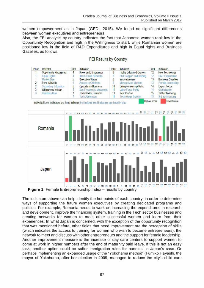
Oradea Journal of Business and Economics, Volume II Issue 1 Published on March 2017
87
women empowerment as in Japan (GEDI, 2015). We found no significant differences between women executives and entrepreneurs. Also, the FEI analysis by country indicates the fact that Japanese women rank low in the Opportunity Recognition and high in the Willingness to start, while Romanian women are positioned low in the field of R&D Expenditures and high in Equal rights and Business Gazelles, as follows:
Figure 1: Female Entrepreneurship Index – results by country
The indicators above can help identify the hot points of each country, in order to determine ways of supporting the future women executives by creating dedicated programs and policies. For example, Romania needs to work on increasing the expenditures in research and development, improve the financing system, training in the Tech sector businesses and creating networks for women to meet other successful women and learn from their experiences. In what Japan is concerned, with the exception of the opportunity recognition that was mentioned before, other fields that need improvement are the perception of skills (which indicates the access to training for women who wish to become entrepreneurs), the network to meet and discuss with other entrepreneurs and the support for female leadership. Another improvement measure is the increase of day care centers to support women to come at work in higher numbers after the end of maternity paid leave. If this is not an easy task, another option could be softer immigration rules for nannies, in Japan’s case. Or perhaps implementing an expanded usage of the “Yokohama method” (Fumiko Hayashi, the mayor of Yokohama, after her election in 2009, managed to reduce the city’s child-care
Oradea Journal of Business and Economics, Volume II Issue 1 Published on March 2017
88
waiting list, the longest in the country at that moment, to zero in just over three years, by bringing private firms into the sector and creating the necessary day care facilities). Based on OECD’s report, in 2014, Japan increased childcare leave benefits from 50% to 67% of the wages (comparable with Romania that has 85% of the average net income over the last 12 months) in support of a better work-life balance and labor market participation for women. Also, the Japanese Government has established a “new certification system for employers who create an employment environment that is favorable to raising children and encourages a better work-life balance” (OECD 2014) In the end, it is important to mention that, if the two countries do not work harder in accepting and promoting women in executive positions, they might lose a big number of high level and well prepared graduates to foreign companies. In Japan, if the international companies understand the necessity of complying with the working needs of Japanese women, such as support and encouragement to continue working after marriage, the same training and promotion opportunities as for their male colleagues, support in career development, no compulsory socialization or client care after work, so that women can also take care of their families (Subhash and Norton 1993), they can benefit greatly from the high number of highly educated Japanese women. In the case of Romanian women, there are many who tend to emigrate, considering the country poor, corrupted and without opportunities (Stanculescu and Stoiciu, 2012), Romania thus losing a high number of well trained and educated women who could contribute to the economic growth of the country. 6. Conclusions The time for change has come. Not using women in the labor force represents a waste of talent, money and time. In both countries analyzed in this article, half or more of university graduates are female and both countries are in need of well-trained executives in order to improve their activities in the fast changing business environment and in the purpose of economic growth. In order for this to happen, the two countries need to find ways of changing the mentality of their own population regarding working women, provide more understanding and support towards working mothers, sharing the household and children rearing responsibilities, better child care services, etc. Programs such as the ones suggested by the Japanese Prime Minister Shinzo Abe to increase the number of women in executive positions in the next years, are a step forward and make way to new perspectives. However, without the legal mechanisms and institutions to monitor and penalize discrimination of any kind against women at work, no major changes are possible. Problems such as maternity harassment (matahara in Japanese) and forcing women to quit working after getting married, not accepting them back on the same position after returning from maternity leave are urgent and need to be dealt with as soon as possible. Other issues are related to the traditional Japanese management systems of lifetime employment, where women are not included, enterprise unions, seniority systems, a group-oriented and risk-adverse orientation, the culture of maintaining the group harmony and conflict avoidance, as the expression shikata ga nai (there is nothing I can do about it) implies and finally the mentality of "the stake that sticks out gets pounded", indicating the conformity of the Japanese society. Romania ranks slightly better on this level, with stricter protective laws and real implementation, support for women to take parental leave and return to continue their work afterwards. Also, the work environment is more relaxed and there is no compulsory after work communication. However, Romanian women face discrimination regarding educational choices, vertical and horizontal occupational segregation, social perception of a woman’s place, difficulty in accessing capital and lack of positive examples, challenges which are also encountered at their Japanese counterparts.
Oradea Journal of Business and Economics, Volume II Issue 1 Published on March 2017
89
Despite their different backgrounds, the Romanian and Japanese women seem to have a similar fate and tend to be hindered in their successful careers by resembling barriers related to societal pressure and male attitudes towards working women. If these aspects will not change, the economies of both countries will have to suffer and will not have the opportunity to gain the economic growth they desire. References Aggarwal, R.. (ed.) (1999), Lituchy, T., Japanese women in the workplace, in Restructuring Japanese business for growth: strategy, finance, management and marketing perspective, Springer science and Business Media, New York.
Brando, Mariko (2006). The dignity of a woman, PHP 新書, Tokyo
Cojocaru, F. G., (2014). Women entrepreneurship – a solution for Romanian economy development. http://www.strategiimanageriale.ro/images/images_site/articole/article_be77209b9ad7c43df9b66aaffa2b9954.pdf. [06.2016]. Cook, A.H., Hayashi, Hiroko. (1980) Working Women in Japan: Discrimination, Resistance and Reform, New York School of Industrial and Labor Relations, Cornell University. Dirk, Van Damme (11 Jan 2016) Is the gender gap in higher education widening? http://oecdeducationtoday.blogspot.kr/2016/01/is-gender-gap-in-higher-education.html. [07.2016]. European Commission Maternity: http://ec.europa.eu/social/main.jsp?catId=1126&intPageId=3261&langId=en. [07.2016]. Global Entrepreneurship Monitor. Japan. http://www.gemconsortium.org/country-profile/76, 2015. (Accessed June 2016). Global Entrepreneurship Monitor. Romania. http://www.gemconsortium.org/country-profile/103, 2015. [06.2016]. Hidaka, T.,(2010) Salaryman masculinity : continuity and change in hegemonic masculinity in Japan, Leiden: Brill ; Biggleswade, Boston. Ishizuka, H., (17 Jul 2014), Are women really ‘shining’ in Japan?, World Economic Forum, https://www.weforum.org/agenda/2014/07/gender-diversity-management-japan/. [07.2016]. Japan: Women in the workplace. (6 July 2015) Financial Times. http://www.ft.com/cms/s/0/60729d68-20bb-11e5-aa5a-398b2169cf79.html#axzz4E0Mjmusn. [07.2016]. Japanese women and work. Holding back the half the nation. (29 March 2014), The Economist. http://www.economist.com/news/briefing/21599763-womens-lowly-status-japanese-workplace-has-barely-improved-decades-and-country. [06.2016]. Kameda, M., (12 Aug 2014). Only 7.4 percent of Japanese companies have female leader. Japan Times. http://www.japantimes.co.jp/news/2014/08/12/business/7-4-percent-japanese-companies-female-leader/#.V4iKSZN97Vo. [06.2016]. Labor force participation rate, female; The World Bank. http://data.worldbank.org/indicator/SL.TLF.CACT.FE.ZS. [07.2016]. Marinescu, C., (15 Febr 2016). Doar 4,5% dintre barbatii romani opteaza pentru un concediu de cresterea copilului (analiza). [Only 4,5% of Romanian men opt for parental leave (analysis)]. Agerpres. http://www.agerpres.ro/social/2016/02/15/doar-4-5-dintre-barbatii-romani-opteaza-pentru-un-concediu-de-crestere-a-copilului-analiza--10-57-57. [07.2016]. Massino, J., (2004) Anonimatul femeii in estetica Romaniei Ceausiste [Women’s anonymity in Ceausescu’s Romania’s aestetics]. Bucharest University. http://ebooks.unibuc.ro/istorie/ciupala/anonimatulfemeii.htm. [01.2016]
Oradea Journal of Business and Economics, Volume II Issue 1 Published on March 2017
90
OECD (2014) Better life index, http://www.oecdbetterlifeindex.org/topics/work-life-balance/. [5.2016]. OECD (2015) Part-time employment rate, women, https://data.oecd.org/emp/part-time-employment-rate.htm#indicator-chart [6.2016]. Pădurariu, Cezar. (2014). Statutul femeii in Romania Comunista. [Woman’s status during Communist Romania.] http://adevarul.ro/locale/iasi/statut-emancipat-1_531b15fe0d133766a8b878a7/index.html. [07. 2016] Piti, M., 2010. Antreprenor “made in Romania” [“Made in Romania” entrepreneur]. Fundatia post privatizare [Post-privatization Foundation]. http://www.postprivatizare.ro/romana/antreprenor-made-in-romania/). [07.2016]. Popescu, I., (8 Mar 2016). How many women do business in Romania and in what sectors. Romania Insider. http://www.romania-insider.com/how-many-women-do-business-in-romania-and-in-what-areas/. [06.2016]. Ramadani, V., Gërguri-Rashiti, S., Fayolle, A., (2015) Female Entrepreneurship in Transition Economies: Trends and Challenges, Palgrave Macmillan. Renshaw, J., (1999), Kimono in the Boardroom: The invisible evolution of Japanese women managers. Oxford University Press, New York Ryan, K., (11 Febr 2015). Maternity Harassment in Japan. The Diplomat. http://thediplomat.com/2015/02/maternity-harassment-in-japan/. [06.2016]. Scarlatescu, M., 2013. Antreprenoriatul in Romania [Entrepreneurship in Romania]. http://sisc.ro/antreprenoriatul-in-romania/. [07.2016]. Stanculescu, M., Stoiciu, V., (2012). The impact of the economic crisis on the labor migration from Romania. http://www.fes.ro/media/publications/Carte_migratiei_EN__final.pdf. Accessed March 2016. [06.2016]. Statistics Japan, http://www.stat.go.jp/english/data/handbook/c0117.htm. (Accessed July 2016). Subhash, D., Norton, M., (1993), Japanese Business. Cultural perspectives. State University of New York Press. The Global Entrepreneurship and Development Institute (GEDI). Female Entrepreneurship Index 2015 Report. https://thegedi.org/female-entrepreneurship-index-2015-report/ [07.2016]. Transparency International Romania, 2015, https://www.transparency.org.ro/politici_si_studii/indici/ipc/2015/IPC2015_TabelRegional_UE_si_WE_RO.pdf [07.2016]. Weber Shandwick (2015), Gender Equality in the Executive ranks: a paradox. The journey to 2030, available at http://www.webershandwick.com/uploads/news/files/gender-equality-in-the-executive-ranks-report.pdf [07.2016] Bio-note Irina Roibu is Assistant Profesor at Hankuk University of Foreign Studies, Department of Romanian Studies, Seoul, South Korea. Her research interests include East Asian Studies. Paula Alexandra Roibu (Crucianu) is Ph.D student at University at „Alexandru Ioan Cuza”, Iași, Doctoral School of Economic and Business Administration. Her main research interests include Economics. The subject of her PhD research is “The Entrepreneurship in economic theory and practice”.
Oradea Journal of Business and Economics, Volume II Issue 1 Published on March 2017
91
EXPLORING THE OBSTACLES AND THE LIMITS OF SUSTAINABLE DEVELOPMENT. A THEORETICAL APPROACH Paula-Carmen Roșca Doctoral School of Economics, Faculty of Economic Sciences, University of Oradea, Oradea, Romania [email protected] Abstract: The term “sustainable” or “sustainability” is currently used so much and in so many fields that it has become basically part of our everyday lives. It has been connected and linked to almost everything related to our living, to our lifestyle: energy, transport, housing, diet, clothing etc. But what does the term “sustainable” really mean? Many people may have heard about sustainable development or sustainability and may have even tried to have a sustainable living but their efforts might not be enough. The present paper is meant to bring forward a few of the limits of “sustainability” concept. Moreover, it is focused on revealing some arguments from the “other side” along with disagreements regarding some of the principles of “sustainable development” and even critics related to its progress, to its achievements. Another purpose of this paper is to draw attention over some of the issues and obstacles which may threaten the future of sustainability. The paper is also meant to highlight the impact that some stakeholders might have on the evolution of sustainable development due to their financial power, on a global scale. Keywords: sustainability; development; limits; criticism; obstacles; disagreements. JEL classification: Q01, Q50. 1. Introduction The idea that the future should be a healthier and a better place for us and for the next generations is known as “sustainable development” and it embraces a growing acceptance that human actions have a serious and negative impact on our planet’s ecosystems. The idea is not new and many researchers studied the phenomenon and a lot of debates took place over this topic, on a global scale, as there were many resistances and refusals along the way. Sustainable development is a concept that integrates several areas that need to be rethought and refocused and involves economic development as much as other areas of human life and activity. After all, the primary aim is to find a way to reconcile the interests of economic development with the social and environment ones (Rojanschi, 2006, Badulescu et al, 2014). One of the first researchers who was focused on studying sustainable development was Mahon Munasinghe who describes sustainable development as:
„a process for improving the range of opportunities that will enable individual human beings and communities to achieve their aspirations and full potential over a sustained period of time, while maintaining the resilience of economic, social and environmental systems. Thus, sustainable development requires both increases in adaptive capacity and opportunities for improving economic, social and ecological systems.”
(Munasinghe, 2007)
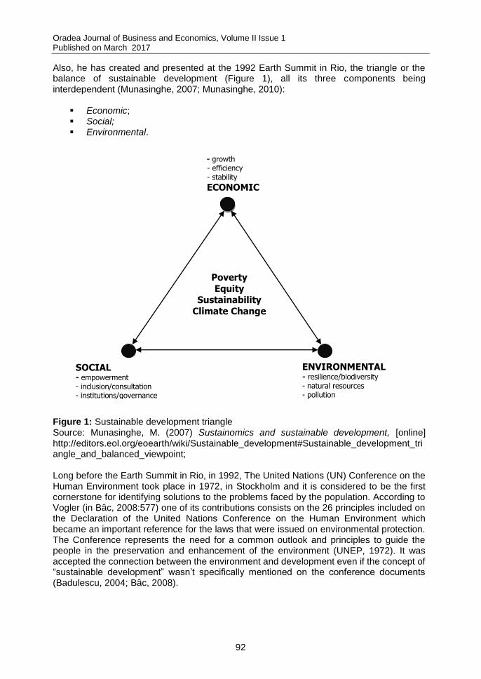
Oradea Journal of Business and Economics, Volume II Issue 1 Published on March 2017
92
Also, he has created and presented at the 1992 Earth Summit in Rio, the triangle or the balance of sustainable development (Figure 1), all its three components being interdependent (Munasinghe, 2007; Munasinghe, 2010):
Economic; Social; Environmental.
Figure 1: Sustainable development triangle Source: Munasinghe, M. (2007) Sustainomics and sustainable development, [online] http://editors.eol.org/eoearth/wiki/Sustainable_development#Sustainable_development_triangle_and_balanced_viewpoint; Long before the Earth Summit in Rio, in 1992, The United Nations (UN) Conference on the Human Environment took place in 1972, in Stockholm and it is considered to be the first cornerstone for identifying solutions to the problems faced by the population. According to Vogler (in Bâc, 2008:577) one of its contributions consists on the 26 principles included on the Declaration of the United Nations Conference on the Human Environment which became an important reference for the laws that were issued on environmental protection. The Conference represents the need for a common outlook and principles to guide the people in the preservation and enhancement of the environment (UNEP, 1972). It was accepted the connection between the environment and development even if the concept of “sustainable development” wasn’t specifically mentioned on the conference documents (Badulescu, 2004; Bâc, 2008).
SOCIAL - empowerment - inclusion/consultation - institutions/governance
ENVIRONMENTAL - resilience/biodiversity - natural resources - pollution
Poverty
Equity Sustainability
Climate Change
- growth - efficiency - stability
ECONOMIC
Oradea Journal of Business and Economics, Volume II Issue 1 Published on March 2017
93
Since then, other meetings, protocols and conferences were organized by UN on the topic of sustainable development:
The Brundtland Report (Our Common Future) - 1987; Rio de Janeiro Earth Summit - 1992; Kyoto Protocol - 1997; The World Summit on Sustainable Development (Johannesburg) - 2002; United Nations Climate Change Conference (Copenhaga) - 2009; United Nations Conference on Sustainable Development, Rio+20 (Rio de Janeiro) -
2012; United Nations Sustainable Development Summit (New York) – 2015.
The contributions of all the above meetings and conferences materialized in protocols, documents, agreements between states are often questioned by some authors and field experts. Despite all the debates, proposals and agreements that took place between states so far, there are several opinions according to which, sustainability, as approached during the last few decades has various drawbacks. The main criticisms are due to the results almost elusive in most areas of sustainable development. Thus, the future of sustainable development has been called into question. Our research is focused on presenting some of these critics and arguments against sustainability, in an attempt to highlight its limits. Our findings refer mainly to disagreements over some of the sustainability principles and critics regarding the vagueness of the concept or the lack of visible improvements throughout time. We also headed our research towards the limitations of the sustainability progress caused by obstacles like terrorism, population growth, lack of consensus regarding climate change etc. 2. Research methodology The main purpose of the research is to identify the issues that have sparked criticism and the arguments underlying them. We focused on finding the main concerns regarding the improvements made until now, if we are on the right path or even if we need to be concerned about something. The research is mostly a theoretical one and is based on other papers and studies written on this topic. The theoretical research is supported also by updated statistical information. For the statistical research we used as data sources, official information published on the webpages of organizations like World Bank, FAOSTAT, World Health Organization or
publications like Fortune 500. The research covers a long period of time, including recent years (2015-2016) and presents comparisons and evolutions throughout time for several indicators (e.g.: global food consumption, people undernourished, comparisons between corporations and national economies regarding revenue/GDP etc.). The findings of our research are split in four sections, starting with the criticism regarding the lack of progress and improvement and even the disagreements over the significance of this phenomenon. Moving forward, the second part presents aspects related to the vagueness of the concept while the last one lists a number of obstacles faced by the humanity in its way to a better future. 3. Research findings 3.1. Disagreements over the sustainability principles Speth (2008) presents some of the limits of sustainability, through the eyes of the environment component. He states that although some improvement was registered, most of the threats linked to the environment that are acknowledged and extensively discussed during all the conferences and summits held on this subject, have worsened. He concludes that the results of more than two decades of international negotiations are deeply
Oradea Journal of Business and Economics, Volume II Issue 1 Published on March 2017
94
disappointing. Treaties and agreements and their associated protocols cannot do the necessary changes. Typically, these agreements are the easiest option for governments to act because they seem impressive but it does not bind to the objectives of the Treaties, objectives are often not followed by the requirements, goals and clear timetables. And even when there are targets and timetables, they are often inadequate and the means of execution are missing (Speth, 2008). Regarding the disagreements, there are a few critics who argue against the principles of sustainable development. According to Beckerman (2002), future generations are likely to be much better off than the present generation due to the contribution of modern technology, which is rapidly increasing now and is more likely to remain so during the twenty-first century. He claims that we shouldn’t ask the present generation to make sacrifices for future generations. The greatest favor that the present generation can do to the future one is to establish peace and security and to ensure the implementation of the principles of human rights and democracy. Other critics believe that sustainable development can be damaging for the poor people. Thus, on the pretext of promoting sustainable development and environmental protection, rich countries are adopting protectionist policies by restricting imports of agriculture, forestry, and other products from developing countries. They also argue that, in the absence of concrete scientific evidence, environmentalists are recommending adopting precautionary principles, thus incurring a very high cost to control climate change, sea-level rise and ozone depletion which may or may not be significant threats to mankind. If such precautionary principles are not adopted, the resources can be utilized to satisfy the basic needs of the poor in developing countries (Rogers, Jalal, Bozd, 2008). 3.2 Denial of exaggerated predictions Another criticism is addressed to the environmentalists who oftentimes show dramatic trends in negative environmental changes and make their points to invest more in the environment. Lomborg (2003) argues that real State of the World is much better and healthier than many environmentalists claim. In the same 2003 study, Lomborg criticized Ehrlich (1968) who stated: “the world will experience starvation of tragic proportion–hundreds of millions will starve to death”. So, although the world population has doubled since 1961, the average calorie intake per capita has increased by 24% globally and 38% in developing countries. The statistics published by World Health Organization regarding food consumption at a global and regional level, reinforces Lomborg’s opinion (Table 1). Table 1: Evolution of global and regional food consumption (kcal per capita/day)
Region 1964 - 1966
1974 - 1976
1984 - 1986
1997 - 1999
2015 2030*
World 2358 2435 2655 2803 2940 3050
Developing countries 2054 2152 2450 2681 2850 2980
Near East and North Africa
2290 2591 2953 3006 3090 3170
Sub-Saharan Africa 2058 2079 2057 2195 2360 2540
Latin America and the Caribbean
2393 2546 2689 2824 2980 3140
East Asia 1957 2105 2559 2921 3060 3190
South Asia 2017 1986 2205 2403 2700 2900
Industrialized countries 2947 3065 3206 3380 3440 3500
Transition countries 3222 3385 3379 2906 3060 3180
*forecast
Oradea Journal of Business and Economics, Volume II Issue 1 Published on March 2017
95
Source: World Health Organization (2003) Diet, Nutrition and Prevention of Chronic Deseases [Online], Available: http://www.fao.org/docrep/005/AC911e/ac911e05.htm; More than that, the statistical data of Food and Agriculture Organization of the United Nations (FAO) proves that starting from 2006, the number of undernourished people is decreasing in all regions including Asia and Africa (Table 2). Table 2: Evolution of the number of people undernourished (millions) (3-year average)
Region 2000- 2002
2002- 2004
2004- 2006
2006- 2008
2008- 2010
2010- 2012
2012- 2014
2014- 2016
Africa 210.2 214.6 214.3 213.6 217.6 218.3 221.4 230.3
Asia 636.6 669.1 679.3 640.1 583.6 547 526.8 511.7
Latin America and the Caribbean
60.4 55.5 50.3 44 40.3 38.3 36 34.3
Oceania 1.3 1.4 1.4 1.3 1.2 1.3 1.4 1.4
World 929.6 959.2 961.7 913.8 857.9 820.6 800.3 792.5
Total 1890 1947 1949 1849 1733 1637 1597 1581
Source: the author based on the FAOSTAT data, [Online], Available http://www.fao.org/faostat/en/#data/FS; 3.3 The Limits and the Vagueness of the Concept Robinson (2004: 375) summarizes his three criticisms of sustainable development in the way it was debated so far, as: “vague, attracts hypocrites and fosters delusion”. Regarding the uncertainties, the author argues that the term “sustainable development” means different things to different people and organizations. The different concepts tend to reflect a variety of agendas, beliefs and conflicts; more than that, the exact meaning of the term is being discussed for more than 25 years. Disappointments and illusions refer to the social limits of growth which are impossible to reconcile with the global industrial production growth. Moving forward, the vagueness of the term opens ample opportunities for "greenwashing"; for example, the term “green” was very often commercialized to justify unsustainable practices and activities. Many if not most of the activities that are in fact not sustainable, can appear as “green” misleading the population for all sorts of marketing tricks. An example of this are green approaches of airports and airplanes such as "EcoFly" or “Project Green Flights" (Pargman and Raghavan, 2014). According to TerraChoice Environmental Marketing (in Dahl, 2010), although greenwashing is a concept known since the mid-1980s, its use has increased significantly in recent years because companies strove to meet the consumers’ demand for greener products. On its third Greenwashing Report (2010) issued on the subject (in the United States and Canada), TerraChoice identified 4744 products making green claims, showing an increase of 73% by comparison to the company’s second report (2009), 95.4% of those products being guilty of greenwashing. Among the multitude of green labels available today, only a few are recognized as highly reliable. Claudette Juska (in Dahl, 2010:6), a research specialist at Greenpeace, thinks that “people have become skeptical of any environmental claims. They don’t know what’s valid and what isn’t, so they disregard most of them.” Anyway, attaching the adjective sustainable to any type of activity - from construction to economic activities or ministries - cannot be suitable because it is hard to believe that all these activities are truly sustainable. He believes it is important to identify and accept the limitations of sustainability, in order to avoid losing the true sense of the term Marcuse (2006).
Oradea Journal of Business and Economics, Volume II Issue 1 Published on March 2017
96
3.4. The Main Obstacles and Challenges on the Path of Change Regarding the barriers that intervene in the path of sustainability, Rogers et al. (2008) offer a more complex list of obstacles that make hard to achieve the goal of becoming a sustainable planet: Terrorism. Worst case scenario concerning terrorism involves a situation in which a terrorist group will get nuclear weapons or other weapons of mass destruction; Climate change. This is a more complex issue due to the lack of consensus on the effects they may experience in the next years; Global food system. Lack of soil fertility is a problem faced by many countries. The use of chemicals is not a solution anymore because "the ground has become a junkie which needs chemicals as it’s no longer able to produce on its own”. Globalization. It has many manifestations of unsustainable behavior. The best example is the "export" of waste and polluting industries to other countries, which globally is not a solution. On the other hand, other opinions support the idea that population growth is the main obstacle to a sustainable society. Bartlett (2006) considers necessary to implement on a global scale, the family planning - and even reducing the aid granted to states that do not have sufficient measures in reducing national population. Another aspect that needs to be taken into consideration is the awareness of the impact that corporations might have on sustainable development. Steger (2004) emphasized the importance of large corporations and their involvement in efforts that are truly sustainable. In order to demonstrate the magnitude of the power owned by corporations, he presented in his work, the results of a study according to which, the aggregate turnover of the top 200 corporations in the world exceeded the economies of all countries of the world minus the cumulative top 10. Doing the same research but using the updated data, for 2015, we found that the situation has improved. Using the statistics published on fortune.com and worldbank.org, we cumulated the revenue of the top 200 biggest corporations in the world and compared it to the economies of all countries of the world minus the cumulative top 10 (based on a comparison of company revenue and country GDPs). We briefly present our research results as follows: -Top 200 corporations sums 18.3 trillion $ in revenue, representing 24.77% of the world GDP (compared to 27.5% in 1999); - The aggregate revenue of the top 500 corporations in the world (27.6 trillion $) exceeded the economies of all countries of the world minus the cumulative top 10 (24.8 trillion $). - Top 500 corporations employ only a tiny fraction of the world’s labor force (1.97%). Having as a starting point Anderson and Cavanagh’s research (2000) for 1999, we made a comparison between top 100 economies in the world and for that, we updated the information until 2015 using the statistical data available on www.fortune.com and www.worldbank.org. As a result, in 1999, 51% of the 100 largest economies in the world was owned by corporations while in 2015, the trend appears to be going in the reverse direction (66% countries, 34% corporations). Even if national economies won more power over the time, the fact that in 2015, 34% of the top 100 economies of the world is owned by corporations, can be considered an alarming statistic. In their research, Anderson and Cavanagh (2000) are bringing into question if these companies are truly providing what’s good for the countries and global society. The conclusion of their research is that widespread trade and investment liberalization have contributed to a climate in which big corporations have registered increasing levels of economic and political power that are out of balance with the real benefits they provide to society. The study presents results of a research conducted by Business Week magazine which revealed that between 72% and 82% of Americans believe that corporations have gained
Oradea Journal of Business and Economics, Volume II Issue 1 Published on March 2017
97
too much power over many aspects of their life and 74% agreed with Al Gore’s criticism of “a wide range of large corporations, including ‘big tobacco, big oil, the big polluters, the pharmaceutical companies, the HMOs’” (Anderson and Cavanagh, 2000). The conclusion is that big companies have a lot of influence over government policy and policy-makers. This is just one of numerous statistics that clearly indicate that active engagement of corporations is essential if the world wants to achieve changes in the patterns of production and consumption or on domestic and international laws that will be needed to align the planet on the path of sustainability. Sometimes, change is considered to be initiated by minorities or intellectual elite who run the risk of being pioneers. So it takes an impulse that can later cause chain reactions. In this way, people become aware of the problems they face and can seek solutions for them. Furthermore, Gorbachev (2006:160) draws attention to the people to exercise their voting power in the political establishment, which should be judged according to their facts, not their words. Therefore, he said, "we need a new Glasnost to inspire citizens to become actively involved in the struggle for a better future." Meadows (2006), believes in the need for a sustainability revolution. Like the Industrial Revolution in the past, it will require decades or centuries to achieve completely, but according to the author, "Sustainability Revolution" has already begun. 4. Conclusion There are a lot of other views regarding the sustainable development and its drawbacks and being such a complex matter, it may be the subject of a broader research. In conclusion, sustainable development is a mixture of many stories, actions, values and perspectives which require the capacity and availability to listen to others and leave aside established opinions. However, lack of information, confusion over cause and effect, no clear vision of sustainability, the underestimation of the impact that some stakeholders (such as corporations) might have on this matter, are only a few of the aspects that require more attention and which indicate shortcomings of our actions and attitudes towards sustainable development. References Anderson S., Cavanagh J. (2000). Top 200. The Rise of Corporate Global Power, Institute for Policy Studies, Washington. Bartlett (2006). `Reflections on sustainability, population growth, and the environment` in Keiner, M. (ed.) The Future of Sustainability, Springer, Dordrecht. Badulescu A., Badulescu D., Bac, D., Șipoș-Gug S., (2014). `Attitudes and intentions of business master students towards sustainable tourism and entrepreneurship`, Amfiteatru Economic, vol. 16, no. 8, pp.891-905. Badulescu, A (2004), Economia turismului, Editura Universităţii din Oradea, Oradea. Bâc, D. (2008). `A history of the concept of sustainable development: literature review` Annals of University of Oradea. Economic Sciences, vol.17, no.2, pp. 576-581. Beckerman, W. (2002). A Poverty of Reason: Sustainable Development and Economic Growth, The Independent Institute, Oakland. Dahl, R. (2010). ‘Green Washing: Do You Know What You're Buying?’Environmental Health Perspect, vol. 118, no. 6, pp. 246-252. Gorbachev, M. (2006). ‘A New Glasnost for Global Sustainability’, in Keiner, M. (ed.) The Future of Sustainability. Dordrecht: Springer. Lomborg, B. (2001). The Skeptical Environmentalist: Measuring the Real State of the World, Cambridge: Cambridge University Press.
Oradea Journal of Business and Economics, Volume II Issue 1 Published on March 2017
98
Marcuse, P. (2006). ‘Sustainability is Not Enough’, in Keiner, M. (ed.) The Future of Sustainability. Dordrecht: Springer. Meadows, D. (2006). Tools for the Transition to Sustainability’, in Keiner, M. (ed.) The Future of Sustainability. Dordrecht: Springer. Munasinghe, M. (2010). ‘Addressing the Sustainable Development and Climate Change Challenges Together: Applying the Sustainomics Framework’, Procedia Social and Behavioral Sciences, no. 41, pp. 6634–6640. Munasinghe, M. (2007). ‘Sustainomics and sustainable development”, [online], Available from: http://editors.eol.org/eoearth/wiki/ Sustainable_development#Sustainable_development_triangle_and_balanced_viewpoint. [12.10.2016]. Pargman, D., Raghavan, B. (2014). Rethinking Sustainability in Computing: From Buzzword to Non-negotiable Limits, [Online], Available from: https://www1.icsi.berkeley.edu/~barath/papers/sustainability-nordichi14.pdf. [12.10.2016]. Robinson, J. (2004). ‘Squaring the circle? Some thoughts on the idea of sustainable development’, Ecological Economics, vol 48, no. 4. Rogers, P., Jalal, K. Bozd, J. (2008). An Introduction to Sustainable Development, Oxford: Earthscan.
Rojanschi, V., Bran, F., Grigore, F., Ioan, I. (2006). Cuantificarea dezvoltării durabile, Bucuresti: Editura Economică. Speth, J.G (2008). The Bridge at the End of the World, London: Yale Univ. Press. Steger, U (2004). The Business of Sustainability, London: Palgrave Macmillan Publishers. World Health Organization (2003). Diet, Nutrition and Prevention of Chronic Deseases [Online], Available from: http://www.fao.org/docrep/005/AC911e/ ac911e05.htm. [19.01.2017]. The World Bank (2017). World Development Indicators, [online] Available from: http://data.worldbank.org/data-catalog/GDP-ranking-table [19.01.2017]. Fortune 500 (2016). [online] Available from: http://beta.fortune.com/fortune500/list. [19.01.2017]. UNEP (1972). Declaration of the United Nations Conference on the Human Environment, [online] Available from: http://www.unep.org/documents.multilingual/default.asp? documentid=97&articleid=1503. [19.01.2017]. FAOSTAT (2017). Food Security Indicators, [online] Available from: http://www.fao.org/ faostat/en/#data/FS. [18.01.2017]. Bio-note Paula-Carmen Roșca, is Ph.D. student at University of Oradea, Faculty of Economics Sciences. Her research interests include general aspects of sustainable development and her main focus for the PhD research is corporate sustainability.
Oradea Journal of Business and Economics, Volume II Issue 1 Published on March 2017
99
THE DOCTORAL SYMPOSIYUM - ORADEA 2016: AN OVERVIEW
Scientific research in economics plays, now more than ever, an important role in investigating issues and generating solutions and models of economic and social development. Moreover, in the contemporary world, development is inconceivable in the absence of sustained research and development activities. Undoubtedly, scientific research must be conducted primarily in higher education institutions, in academic and research laboratories. In this context, the scientific research of young people - students, master students and, in particular PhD students - acquires special meanings and its fostering a duty of honour to academics and supervisors at all levels. Recognizing and understanding all these realities, in the Faculty of Economic Studies and Doctoral School of Economic Sciences at the University of Oradea, there have been encouraged and supported the efforts and steps on the path of doctoral scientific research. Thus, since 2010 there is organized an Annual Doctoral Symposium of PhD students in Economics and related fields, and papers carefully selected after the peer-review process were published in a volume that encompassed the scientific contributions. On 23
rd of November, our Doctoral School organised the 7
th edition of the Doctoral
Symposium. A number of 52 papers were registered for the Conference, and they were presented on 5 panels, dealing with topics related to Microeconomics and Economics of the firm, Entrepreneurship and SMEs, Tourism and services, Macroeconomics etc. All submitted contributions were double-blind reviewed and 46 of them were accepted for publication in the proceeding book, namely the 4
th issue of the journal Emerging Markets
Economics and Business. Contributions of Young Researchers. Proceedings of the 7th Conference of Doctoral Students in Economic Sciences.
Let me congratulate all participants, and especially those authors whose contributions were
published. Moreover, few selected authors were invited to submit extended versions of their
contributions for considering in Oradea Journal of Business and Economics. They are
published in this issue, on the Papers selected from the Doctoral Symposyum 2016 section.
We have the strong belief that young researchers are, by training and audacity, a tank of
opinions, viewpoints, and especially solutions and proposals, and aware that they should be
encouraged and promoted as to enable them to confirm the hopes of their teachers and
supervisors.
Last but not least, let me address special thanks to the members of the Scientific Board, to reviewers, to the members of the Organizing Committee, and to all generous fellows who supported the Annual Doctoral Symposium held on 23
rd of November 2016 at the University
of Oradea. Oradea, March 2017 Professor Alina Badulescu Dean of the Faculty of Economic Sciences – University of Oradea President of the Doctoral Symposium