Option Values, Switches and Wages - An Analysis of the Employment Guarantee Scheme in India

Pasquale Scandizzo*, Raghav Gaiha** and Katsushi Imai***

*University of Rome “Tor Vergata”, **University of Delhi, and ***Royal Holloway, University of London

***Corresponding Author: Katsushi Imai (Dr) Department of Economics Royal Holloway, University of London Egham, Surrey TW20 0EX, UK Telephone: +44-(0)1784 -443309 Fax: +44-(0)1784-439534 E-mail: katsushi.imai@rhul.ac.uk

2

Abstract Consistent with the theory of real options, it is argued that the value of the Employment Guarantee Scheme (EGS) in the Indian state of Maharashtra and its impact on workers’ behaviour do not depend so much on its income supplementation as on enlargement of opportunities in an uncertain environment of the local labour market. The choice between the EGS and other activities in rural areas is modelled in a dynamic optimisation framework that takes into account a fixed wage rate and certainty of employment under the former and a stochastic wage rate in the latter. Besides, entry and exit costs of various employment options are taken into account. Finally, allowance is made for volatility of regular labour market activities (e.g. agricultural wage earnings). The predictions of this model are validated with the help of a panel household survey in a semi-arid region of south India. If this analysis has any validity, the incentive case for rural public works schemes such as the EGS in terms of screening and deterrent arguments, premised on a fixed wage rate differential, needs to be reformulated. Key words: options, uncertainty, entry and exit costs, incentives. JEL codes: D3, D8, H5, I3, J2.

3

Option Values, Switches and Wages - An Analysis of the Employment Guarantee Scheme in India

Pasquale Scandizzo, Raghav Gaiha and Katsushi Imai1

1. Introduction

Much of the earlier work focuses on the targeting and poverty alleviating potential of the

Employment Guarantee Scheme (hereafter EGS) in the Indian state of Maharashtra (e.g. Gaiha,

2001, Ravallion, 1991, Ravallion and Datt, 1995). Attention is given to various mechanisms

through which it impacts on the rural poor. These include direct transfer benefits as well as

indirect ones through a positive effect on agricultural wage rates. A point of departure of the

present study is the focus on switches into the Employment Guarantee Scheme in the Indian

state of Maharashtra in a framework consistent with the theory of real options. This theory

appears relevant for the problem on hand, because the value of the EGS scheme and its impact

on workers’ behaviour do not depend so much on its effects as an income supplement, but on the

enlarged set of opportunities that it provides in the uncertain environment of the local labour

market and farm and non farm activities. Thus, rather than actual increase in income and

employment, the EGS promises potential increases of these variables for given levels of

volatility in the regular labour market, or, alternatively, potential decreases in volatility for given

levels of income and employment. As in most insurance schemes, these effects, in turn, may

change workers’ behaviour in a way that may not be fully consistent with “ex ante” conditions.

For example, the extent to which workers diversify their portfolio of activities may be reduced

and a larger proportion of workers may participate in the regular labour market, rather than in

own farming or non- farm activities, since the EGS provides a form of employment of last resort,

at an institutional wage, that can be readily used to cover unemployment and wage risks.

The choice between the EGS and other activities in rural areas-including farm and non-

farm- is modelled in a dynamic optimisation framework that takes into account a fixed wage rate

and certainty of employment under the former (for a fixed period of time) and a stochastic wage

1 University of Rome “Tor Vergata”, University of Delhi, and Royal Holloway, University of London, respectively.

4

rate in the latter, over different seasons.2 Besides, entry and exit costs of various employment

options- specifically, the EGS and farm and non-farm activities- matter. Allowance is also made

for volatility of regular labour market activities – in the present case, agricultural wage earnings.

The focus therefore is on switches between these alternatives on the basis of a (discounted ) cash

flow analysis that encompasses these factors. Some interesting insights into participation in the

EGS emerge. The higher the EGS wages, for example, the higher would be the proportion of

higher income workers for two mutually reinforcing reasons: higher EGS wages (net of entry

costs) will induce more higher income workers to opt out of other labour market activities in

favour of the former; and higher EGS wages would also make fewer higher income participants

to opt out of this scheme in response to expected wage increases in other labour market

activities. Moreover, since higher expected incomes can be used to offset entry and exit costs, the

EGS would also tend to select a disproportionately higher proportion of higher income workers,

as they can afford to switch back and forth more easily than less affluent ones. Indeed, some of

these insights may throw new light on and explain better the worsening of mistargeting of the

EGS during the 1980s- a period marked by a sharp rise in EGS wages rates.3 But, more

generally, premised as they are on a given wage rate in regular labour market activities, the

screening and deterrent arguments that are invoked to support workfare programmes- of which

the EGS is a special case – lose some of their appeal.4

Guided by the option value model developed here, an empirical analysis of switches into the

EGS and non-farm activities is carried out, as these seem important in the context of a semi-arid

2 This is a significant point of departure from an earlier model of intrahousehold time allocation across various activities such

as wage labour, own farm work, self-employment, domestic work, etc. as a function of a vector of exogenous variables and the time spent on the EGS. The problem is one of household utility maximisation in which employment under the EGS is rationed. Although an interesting model, it has two limitations. One is that the entry and exit costs of various options are not considered. A second limitation is that rationing under the EGS became a serious concern only after the wage hike of 1988. This is an important issue as the data analysed cover the period 1979-84. For details, see Ravallion and Datt (1995).

3 For illustrative evidence on a worsening of the mistargeting of the EGS, see Gaiha (2000, 2001). 4 In an influential contribution, Besley and Coate (1992) elaborate the rationale of workfare programmes, given the

distribution of the population into low and high ability groups. The objective of workfare is to minimise the cost of poverty alleviation subject to the constraint that everybody obtains a fixed minimum income, z. The transfer package (b, c), where b refers to transfer amount and c denotes a cost in terms of a work-requirement, may induce high ability (and the more affluent) individuals to masquerade as low ability persons to benefit from it. Besides, the cost of poverty alleviation may rise to the extent low ability (poor ) individuals reduce their hours of work in the regular labour market. A solution is worked out in terms of a particular work-requirement, c*, that enables low ability individuals to obtain the minimum income and discourages high ability individuals from claiming the transfer amount. A limitation of this analysis, however, is that wage rates in the regular labour market and the benefits of workfare are taken as given. The point of the present analysis is to focus on choices in a context of changing option values.

5

region in south India.5 While consistent with a basic insight of the model, there are some striking

differences in the underlying factors.

The scheme is as follows. In Section 1, salient features of the EGS are described. This is

followed by a short description of the ICRISAT panel survey in Section 2, on which the

switching analysis is based. Section 3 contains a condensed version of the option value model of

participation in different activities including the EGS. In the next Section, an econometric

analysis of switching is given. The paper concludes with a brief review of the main findings from

a broad policy perspective.

Section 1

EGS – Salient Features6

In a large part of India – especially in the semi-arid region to which Maharashtra belongs –

agriculture is a highly seasonal activity. During the lean periods, large sections of rural

households eke out a bare subsistence through short spells of mostly unremunerative

employment. If employment opportunities expanded, the severity of hardships would lessen.

Motivated by this concern, Mr. V. C. Page initiated the EGS experimentally in 1965. (In fact, it

was known for some time as the Page scheme). It was subsequently expanded as part of an

integrated rural development project, culminating in the EGS Act (No. XX of 1978) and its

implementation in Maharashtra in 1979. From a modest beginning, the EGS expanded rapidly

into the most important poverty alleviation programme in Maharashtra.

The scheme guarantees that every adult who wants a job in rural areas will be given one,

provided that the person is willing to do unskilled manual work on a piece - rate basis.7 Self-

selection of the poor is built into the EGS. First, no choice of work is offered. Secondly, until

1988, the wage rate was usually below the agricultural wage rate.8 Thirdly, as the guarantee

5 Other related issues are addressed in a companion piece (Scandizzo, Gaiha and Imai, 2003). 6 This draws upon GOM (1997). 7 However, a person who is between 15-18 years old can be given employment if there is no earning member in the family. 8 Following the High Court directive, the EGS wage rate was hiked in conformity with the Minimum Wages Act. The piece-

rates for different types of manual/unskilled work are so fixed that an average person working diligently for 7 hours a day would earn a wage equal to the minimum wage prescribed for agricultural labour for the concerned zone, under the Minimum Wages Act (GOM, 1997).

6

holds at the district level, a person may be required to travel a long distance for a few days of

temporary work.

The employment seeker is required to work for a minimum of 30 days on the site assigned. The

person must present himself/herself for work within 7 days of offer of work. Failure to provide

employment within 15 days of registration entitles the person to an unemployment allowance (of

Rs.2 per day).9 Ex-gratia payment up to Rs.10, 000 is admissible in case of death or disablement

of a worker on the site. Some amenities provided on the site include potable water, crèches,

resting place and first aid.

The scheme operates through identification of projects which must satisfy two criteria: they

must be labour – intensive and create productive assets. The labour – intensity criterion is

defined rather strictly- the ratio of cost of unskilled labour to equipment, materials, supervision

charges and so on must be 51:49 or higher.10, 11 Productive works are, however, somewhat

loosely defined as those which directly or indirectly lead to an increase in production or which, if

not undertaken, would cause production to decline. With a view to minimising the recurrence of

droughts, priority is given to moisture conservation and water conservation works (e.g.

percolation and storage tanks). Other priorities are soil conservation and land development

works, afforestation, roads, and flood protection schemes. It is mandated that work under the

EGS should be so organised that it does not interfere with normal agricultural activities. Also,

this scheme is not activated when work is available on other plan or non-plan works in

progress.12

9 Hirway and Terhal (1994) draw attention to the use of an elaborate procedure which involves completing several documents,

contacting several different persons, and exasperating bureaucratic negligence and bribery. Consequently, the poor suffer more. To illustrate, lack of coordination between technical and revenue departments often results in delays in execution of EGS projects, forcing the poor to seek alternative sources of employment.

10 This is down from 60:40. A few exceptions include canal works of medium and major irrigation projects which involve rock cutting.

11 Often as a consequence of inflation of material costs some of these are deliberately included in labour costs in order to maintain this norm (Dev, 1993)

12 New projects under this scheme are undertaken only when (i) at least 50 labourers are available, and (ii) they cannot be absorbed in on-going works. However, exceptions can be made for works in hilly areas (GOM, 1997).

7

In recent years, some changes in the composition of EGS projects have occurred. These include

Shram Shaktidware Gram Vikas (integrated village development), promotion of horticulture and

subsidies for construction of wells.13

Over the period 1980-97, there was a decline in EGS participation – the person days of

employment fell from 20.55 crores to 9.01 crores14. The expenditure (at constant prices) also fell

over this period – from Rs.30.17 crores to Rs.24.66 crores. Although participation fluctuated,

there was a sharp reduction in 1989, following the hike in the EGS wage rate. Between 1987-89,

there was a reduction in person days of employment of over 5.50 crores. A large part of this

reduction was due to rationing.15 Soon after there was a gradual rise in EGS participation until

1993, followed by a steady decline in subsequent years.16 Considering that the peak of 1980 has

not been surpassed and the gap between it and participation has widened considerably –

especially during the 1990s – it may be inferred that the importance of the EGS as a

supplementary source of employment has diminished in recent years. However, as argued

elsewhere, the EGS continues to perform an important income stabilising role in backward

regions.

EGS employment continued to peak during the slack period i.e. April - June. Although the mean

EGS participation (about 2 lakhs/0.2million) remained unchanged over the period 1991-96, the

coefficient of variation declined slightly – from 53.24 to 49.11. EGS employment was slightly

more evenly spread from its peak in 1996 relative to 1991. Whether in fact this is a manifestation

of the changing composition of EGS activities cannot be ruled out. Digging of wells, for

example, is often spread over a few months as the subsidy is released in instalments at different

stages of completion. Since some small farmers are unable to raise loans to supplement the

subsidy quickly, the construction gets delayed. If this trend continues, EGS may have a stronger

effect on agricultural wage rate through a spillover of its activities into busier months.17

13 For details, see Gaiha (2001). 14 A crore is equivalent to 10 million. 15 About 50 per cent of the reduction in EGS participation between 1988 and 1989 was a direct consequence of the lowering of

the EGS expenditure and the hike in the wage rate. Taking this as an approximate measure of rationing, it follows that the extent of rationing was large. For details, see Gaiha (1997). Ravallion et al. (1993), however, attribute 86 per cent of the reduction to rationing.

16 Except for 1996 when there was a slight rise in EGS participation. 17 For an analysis of the effect of EGS on agricultural wage rate, see Gaiha (1997).

8

Section 2

ICRISAT Panel Survey

Agroclimatologically, the SAT includes those tropical regions where rainfall exceeds potential

evaporation four to six months in a year. Mean annual rainfall ranges from about 400 to 1,200

mm. India’s SAT is vast and covers about 15 to 20 large regions, each embracing several

districts.

Based on cropping, soil and climatic criteria, three contrasting dryland agricultural regions were

selected by ICRISAT: the Telengana region in Andhra Pradesh, the Bombay Deccan in

Maharashtra, and the Vidarbha region also in Maharashtra. Three representative districts viz.

Mahbubnagar in the Telengana region, Sholapur in the Bombay Deccan and Akola in the

Vidarbha region were selected on rainfall, soil and cropping criteria. Next, typical talukas (i.e.

smaller administrative units) within these districts were selected, followed by the selection of 6

Fig.1 Monthly EGS Attendance in 1991 and 1996

0

0.5

1

1.5

2

2.5

3

3.5

4

Jan Feb Mar Apr May Jun Jul Aug Sep Oct Nov DecMonth

Pers

on D

ays

(Lak

hs)

90-91

95-96

9

representative villages within these talukas. 18 Finally, a random stratified sample of 40

households was selected in each village. This comprised a sample of 30 cultivator and 10

landless labour households. To ensure equal representation of different farm size groups, the

cultivating households were first divided into three strata, each having an equal number of

households. A random sample of 10 households was drawn from each tercile. 10 landless labour

households were also randomly selected. Landless labour households were defined as those

operating less than half an acre (0.2 ha) and whose main source of income was agricultural wage

earnings. All households were interviewed by investigators who resided in the sample villages,

had a university degree in agricultural economics, came from rural backgrounds, and spoke the

local language.

A fixed sample size of cultivator and landless labour households in each village means that the

sampling fractions and relative farm sizes that demarcate the cultivator terciles vary from village

to village. The likelihood that a village household was in the sample ranged from about one in

four in the smaller Akola villages to about one in ten in the larger Mahbubnagar villages.

Landless labour households are somewhat underrepresented in the sample. On average across the

6 villages, they comprise about one-third of the households in the household population of

interest, but their share in the sample is only one-quarter. However, since their mean household

size is less than that of cultivator households, a one-quarter representation is a fair reflection of

their presence in the individual population of interest (Walker and Ryan, 1990).

The data collected are based on panel surveys carried out at regular intervals from 1975 to 1984

covering production, expenditure, time allocation, prices, wages, and socio-economic

characteristics for 240 households in 6 villages representing 3 agro-climatic zones in the semi-

arid region in South India. Given the agro-climatic conditions and purposive selection of the

villages, the VLS data are not representative of all of rural south India or, for that matter, even of

its semi-arid region. Nevertheless, the longitudinal nature and richness in terms of variables

included are what make the ICRISAT VLS data unique.

18 Two villages in each district were selected: Aurepalle and Dokur in Mahbubnagar, Shirapur and Kalman in Sholapur, and

Kanzara and Kinkheda in Akola.

10

As part of the ICRISAT VLS, detailed data on time allocation, especially time spent on public

employment schemes, were collected continuously for 3 villages from the sample households for

the period 1979 to 1984. Of these, 2 (Shirapur and Kanzara) are located in Maharashtra where

the EGS operates. Some of the data files (including those covering the EGS) were updated for

1989. Given the sample design, 12 households were selected randomly from each stratum in the

sample villages. However, only a fraction of the original panel of households could be retrieved.

The present analysis is based on the samples for these two villages and mainly on panel data

collected over the period 1979-84.

Section 3

The Model

The traditional approach to the analysis of employment programmes has considered the

benefits of a separating equilibrium, based on the self selection characteristics of the work -

salary combination (see, for example, Besley and Coate, 1992). In a situation of dynamic

uncertainty, however, we may conjecture that self selection may be less effective, for several

reasons. First, rather than acting on a once – and – for - all allocation of labour, the employment

programme may motivate workers to switch back and forth between the programme and the

labour market in response to threats and opportunities provided by stochastic wages. Because

higher skilled workers are better off economically and more secure in their market positions,

they may be expected to afford entry and exit costs much more easily than low skilled workers.

While its impact is more difficult to hypothesise, uncertainty appears to be an additional,

important factor in determining differential behaviour between poorer and richer workers, since,

while higher wages may be more volatile, lower wages are generally associated with higher risks

of unemployment.

In order to explore these factors and their impact on the EGS, we have resorted to the use of real

option theory. This is a recent innovation in decision theory, which promises to be of great

relevance to analyse and model all problems where decisions are taken, not only under

conditions of imperfect information, but also of dynamic uncertainty. This last term indicates a

situation where uncertainty evolves over time, as a consequence of the new information that

becomes available as sequences of different states of nature materialise. Unlike traditional

11

decision making analysis, which concentrates exclusively on expected present values of future

benefits and costs, methodologies based on real option theory are based on the idea that the

decision maker holds one or more “options”, i.e. rights, but not obligations, to undertake certain

actions whose outcomes are uncertain. As a consequence, these methodologies focus on the risks

and opportunities arising from the uncertain unfolding of events over time.

In the case of an agricultural worker, in particular, the traditional analysis considers his

decision problem as one of optimal allocation of his labour resources, given certain expectations

on the levels of variables, such as wage levels and the probability of finding employment, in

agricultural and non- agricultural markets. According to real option theory, we consider instead

the worker to be endowed with a real option reflecting the working opportunities open to him,

given his present status. In particular, we consider the case of an agricultural worker who may

choose to allocate his labour supply to two alternative uses. On one hand, he may work in the

regular market for a wage whose size depends on market conditions as well as on the probability

and the length of employment. On the other hand, he may decide to join an employment scheme

with a fixed wage and a known portion (possibly all) of his employment time. Joining the

scheme, however, will entail a cost for three reasons: first, it will cause average employment

time in the formal market to fall; second, it will entail administrative expenses (red tape) in the

form of money and time loss; third, it may cause a loss of reputation of the worker on the formal

market.

We assume that participation and exit costs consist of commitment of non-recoverable resources

and that workers decide for every period (say, different seasons) the regime that they will follow,

by predicting the discounted cash flow (DCF), possibly adjusted for risk aversion, that they will

obtain by choosing one of the employment alternatives. For simplicity, we assume that the

worker evaluates his position as if the corresponding income stream were to last indefinitely19.

We model the employment in the regular market as a search process, whereby the worker

samples jobs for openings and salaries from an underlying random distribution. Within a given

interval of time (for example, a season), wage income in the regular market is assumed to

19 It would be possible to assume that the worker expected net present value were calculated with reference to a given predicted duration of the job (for example, up to the end of the season), but this would not add anything to the analysis, while making the notation more cumbersome.

12

change, in such a way that the variance of mean income shift, expressed in percentage terms,

grows linearly with time, as participation in the labour market increases and labourers confront a

higher degree of job and task differentiation. Employment in the regular market is thus assumed

to yield a net cash flow y evolving according to a stochastic process of the geometric, Brownian

motion variety with zero drift:

ydzdy σ=)1( ,

where σ2 is the variance and dz is a normally distributed random variable such that Edz=0 and

dtEdz =2 .

The option to participate in the public employment scheme can be considered a “put” option, i.e.

a faculty, given to the workers employed in the regular labour market, to join the programme,

should the regular salary or wage (or the probability of employment) fall below a certain critical

level20. The value of such an option, F(y), can either be determined by replicating it with a

portfolio of assets and liabilities (see Dixit and Pyndick, 1994, p.189) or, more simply, by using

dynamic programming. The Bellman equation, in fact, prescribes that, in the so called

“continuation region”:

)()()2( yEdFyF =ρ

where ρ is an appropriate rate of discount reflecting the worker’s opportunity cost for delaying

consumption as well as his degree of risk aversion.

Equation (2) states that, in order to maximise the present value of the option, the worker is to

equate, in the continuation region (that is, at the margin between holding and exercising the

option), the value that he would obtain by exercising the option, to the expected present value of

the future capital gains obtained by holding the option. This equation may be used to determine

20 More generally, we can assume that the stochastic process y concerns the income obtained by the worker by dividing his labour among on farm and off farm activities. Note also that regular market salary is used synonymously with wages.

13

the functional form of the option value function. After applying Ito's lemma, in fact, it yields a

partial differential equation whose general solution is:

2

21

1)()3( ββ yAyAyF +=

where A1 and A2 are constants determined by boundary conditions and β1 and β2 are, respectively,

the positive and the negative root of the characteristic equation:

( ) 012

)4( 2 =−− σββρ

We consider the case in which the worker is supposed to change his status only once in

each season. In this case, we can think of the options available to the worker as triggered by a

spline of stochastic processes of the same type as in equation (1), but whose parameters change

at each turn of the season. In this case, the worker’s problem becomes a sequential one

(Knudsen and Scandizzo, 2002). Exit from the programme and entry into the programme have to

meet the two “value matching” conditions (Dixit and Pindyck, 1994, p.218):

(5) 1 1 21 1 2

1 1

i i

tn ns

i i e i i ei it

w C A y y e ds A y A yτ

τ τ τβ β βρτ τ τ τ τ τ τρ

+ + −−+ + + +

= =

− + = + +∑ ∑∫

(6) iiii

n

i

T

tt

suii

n

iu yAEdseyyAyAw +++

++=+

−+++

=++ ∑∫∑ +−=++ τ

τ

ττ βττ

ρτ

βττ

βττρ

11111

211

2111

where τ indicates the low season, with duration from 0 to τt , and 1+τ the high season, with

duration from 1+τt to T and the subscripts e and u denoting, respectively, entry and exit levels

from the programme. Expression (5) states that at any time t the worker decides to join the

programme, if the expected income from the programme over the same time span, minus entry

costs, plus the value of the option to go back to the market in future seasons equals his expected

income from remaining in the (slack season) labour market, plus the value of the option to join

14

the programme at any time in the future within the slack season, plus the value of the options to

enter the market in any of the next seasons. Because the options to enter the labour market in any

of the future seasons are common to both conditions (i.e. being in the market and being in the

programme), their expression drops out, so that equation (5) depends only on the option to join

the programme.

Equation (6), on the other hand, states that, during the busy season, at any time tt +τ the worker

may switch from the programme back to the labour market. At the time of the switch, the

discounted value of his income from the programme over the remaining part of the season plus

the value of the options to re –enter the labour market in the same season, or in one of the future

ones, must equal the expected value of his income from the market minus re –entry costs, plus

the value of the option to enter again the market in the next season or in any of the future ones.

Applying the smooth pasting condition to the equation for the th−τ season, (5), we obtain:

(7) )1)((12

2τρρ

τ

ττ

ρββ

ρ tte

eeCwy

−− −−

+=

Thus, the entry level of income that causes the worker to join the programme is higher, the

higher is the programme wage, the lower are programme entry costs, the closer the timing to the

end of the season, and the lower is the uncertainty (the higher the beta parameter)21. Similarly, if

we consider the condition to exit the programme (i.e. 6), applying again the smooth pasting

condition and substituting into (6):

21 To see the relation between entry level and uncertainty, differentiate equation (7) with respect to σ , using also the characteristic equation (4) to obtain:

0)241)(

)1(1)(1)(()( 2

222

≤++−

−−= −− σσρ

βρρ τρρ

ττ

dee

Cwyd tte A symmetric result obtains for equation

(8):

0)241)(

)1(1)(1)(()( 2

21

211

11

≥+−−

+=++

−−+

+σ

σρ

βρρ ττρρ

ττ

dee

Ewyd Ttu .

15

(8) )1)((1 1

11

111Tt

u

eeEwy

ρρτ

τττρβ

βρ −−

+

++

−+

−=

+

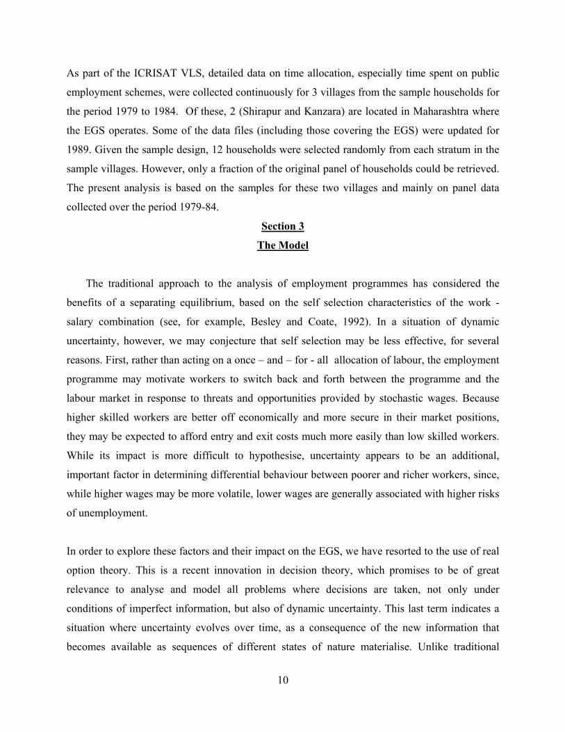
Expression (8) indicates that the salary at which the worker decides to re-enter the market in the

busy season is higher the higher the programme wage, the higher the re-entry costs, the closer the

timing to the end of the season, and the higher is the uncertainty.

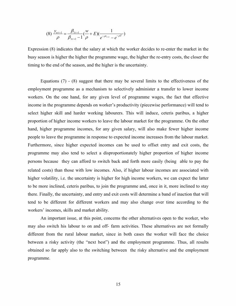
Equations (7) - (8) suggest that there may be several limits to the effectiveness of the

employment programme as a mechanism to selectively administer a transfer to lower income

workers. On the one hand, for any given level of programme wages, the fact that effective

income in the programme depends on worker’s productivity (piecewise performance) will tend to

select higher skill and harder working labourers. This will induce, ceteris paribus, a higher

proportion of higher income workers to leave the labour market for the programme. On the other

hand, higher programme incomes, for any given salary, will also make fewer higher income

people to leave the programme in response to expected income increases from the labour market.

Furthermore, since higher expected incomes can be used to offset entry and exit costs, the

programme may also tend to select a disproportionately higher proportion of higher income

persons because they can afford to switch back and forth more easily (being able to pay the

related costs) than those with low incomes. Also, if higher labour incomes are associated with

higher volatility, i.e. the uncertainty is higher for high income workers, we can expect the latter

to be more inclined, ceteris paribus, to join the programme and, once in it, more inclined to stay

there. Finally, the uncertainty, and entry and exit costs will determine a band of inaction that will

tend to be different for different workers and may also change over time according to the

workers’ incomes, skills and market ability.

An important issue, at this point, concerns the other alternatives open to the worker, who

may also switch his labour to on and off- farm activities. These alternatives are not formally

different from the rural labour market, since in both cases the worker will face the choice

between a risky activity (the “next best”) and the employment programme. Thus, all results

obtained so far apply also to the switching between the risky alternative and the employment

programme.

16

In order to see more clearly what the results obtained imply for programme participation,

assume that at the beginning of the year all workers make their decision by comparing the

realized value of y (i.e. the salary offered on the labour market for their skill group) with the

entry value ey . For the same skill group, we will thus have a participation rate equal to 0 if the

wage in the labour market is above the critical value and 100 per cent otherwise. Similarly, if the

market wage changes are such that it is no longer remunerative to stay in the regular market

compared to the programme, participation would revert to 100% . For any given skill group, the

number of switches to and from the programme should be a function of the entry and exit critical

levels of the stochastic market wage. More specifically, denoting by te and tu the number of

switches respectively into and out of the programme at time t for workers, respectively, in the

labour market or in the employment programme, we can write: ))((1 ettt yGFee += − and

))(1(1 uttt yGHuu −+= − , where )(yGt is the distribution function of the market wage at time t

and (.)F and (.)H are two functions with positive first derivative. In other words, for any given

interval of time, the number of workers switching from the market into the programme should be

a positive function of the probability that market wage is below the programme entry level, ey ,

while the number of people switching out of the programme should be a positive function of the

probability that the market wage is above the programme exit level, uy . By assumption, the

wage distribution is log-normal with mean equal to 0y and variance equal to )1(22

0 −tey σ so

that, if this distribution corresponds to the true income distribution over time, we should observe

that (prob )(()))((log 2iit yhtyhy φσ =≤ , where ,0/)(' ≥∂∂= ii yyhh uei ,= .

By integrating the two difference equations corresponding to te and tu , for t = T, where t

denotes the numbers of units of time considered (for example, the number of working days in a

year), we obtain:

(9) ),,,,())((00

tCwyFyGFe iT

T

i

T

tetTT σ−

==− ∑∑ == , where the expected pattern of signs for the

partial derivatives is, according to (7): ),,,,( +−−+− .

17

(10) ∑∑=

−=

− =−=T

iiT

T

tutTT tEwyHyGHu

00),,,,())(1( σ , where the expected pattern of signs is,

according to (8): ),,,,( −−+−+ .

Equations (9) and (10) can be tested against the empirical data by nesting them in a regression

model of the type:

(11) Tjj

Tj

T

ijjjjjjiTTj XbECrwyFe νσ ++= ∑∑

=−

0, ),;,,,(

where j denotes the j-th worker, TjX a vector of shifters and Tjν a well behaved random

disturbance and r is the interest rate or any other acceptable proxy for the worker’s subjective

discount rate.

Section 4

Estimation and Results

(a) Wage Equation

The ICRISAT panel survey does not contain estimates of wage rates for farm and non-farm

activities and the EGS. As these variables have an important role in the option value model, we

have constructed two alternative sets. In the first set, actual wage earnings in these activities are

divided by the number of days worked by each individual in a year and then ratios of wage rates

are computed. In the second, ratios of wage rates in the EGS and in farm activities, and in non-

farm and farm activities are posited to be endogenous to individual, household and village

characteristics. A random-effects Tobit specification is used to estimate the wage ratio functions,

as shown below.

As specified in equation (12), the ratio of EGS and farm wage rates is determined by a health

(12) Wegs itv /Wagr itv = fitv (H itv, S itv, A itv, B itv, V itv, R tv,,αiv)

indicator viz. body mass index, BMI, denoted by H, a schooling index (number of years) denoted

by S, a vector of socio-demographic characteristics (viz. age, gender, caste, whether married),

denoted by A, other household characteristics (viz. schooling and occupation of household head,

household debt) denoted by B, a measure of wealth (landowned or net worth) denoted by V, a

18

measure of aggregate risk faced by households (viz. coefficient of variation of monthly rainfall)

denoted by R, an unobserved factor (say, ability) denoted by α, and i indexes individual, t

represents year ((t= 1 for 1979, ---, t=6 for 1984) and v denotes village.

As shown in equation (13), a similar set of factors influences the ratio of off or non farm and

agricultural wage rates except that there are a few interaction terms involving the gender

(13) Woff_farm itv /Wagr itv = fitv (H itv, S itv, A itv, B itv, V itv, R tv,,αiv)

dummy and a few other explanatory variables.

Column (a) of Table 1 contains the results on the determinants of the ratio of EGS and

agricultural wage rates. While the BMI and its square do not influence this ratio, age has a

negative effect. This is plausible given that EGS wage rates are piece rates calculated on the

basis of work done. The female dummy has a negative coefficient, implying much lower wages

for female participants in the EGS. Relative to the lowest caste individuals, the medium low

caste individuals have higher wage ratios presumably as a result of higher EGS wage rates.

Individuals belonging to agricultural labour households also have higher wage ratios – especially

because of higher EGS wage rates. The lagged unemployment rate has a positive coefficient,

implying a stronger dampening effect of unemployment on farm wage rates of a lowering of

reservation wage rates22. The overall specification is validated by a Wald test.

Column (b) of Table 1 contains results on the determinants of the ratio of non-farm and farm

wage rates. As both wage rates are market determined, some determinants of this ratio are likely

to be different. Both high and medium high caste individuals have significantly higher wage

ratios than those belonging to the lowest castes. Schooling has a negative coefficient, presumably

as a result of a positive effect on agricultural wage rates. Individuals belonging to agricultural

labour households have a significantly higher wage ratio. The underlying reason is unclear. A

higher debt is associated with a lower wage ratio, consistent with (relatively) unattractive non-

farm wage options. The dummy for Shirapur has a positive coefficient presumably because of

19

low farm wage rates in the more backward of the two ICRISAT villages. The measure of

aggregate risk (i.e. the cv of monthly rain ) is associated with a higher wage ratio, reflecting a

risk premium. The lagged unemployment rate also has a positive coefficient, mainly because of

a stronger dampening effect on farm wage rates. Female dummies interacted with caste and

Shirapur dummies have negative coefficients, implying significantly lower wage ratios. The

overall specification is validated by a Wald test.

(b) Switching Equations

The number of switches between different activities over the entire sample period of six years

(1979-84) is calculated as follows: total number of switches of all individuals in the workforce

aggregated over 6 years/ total number of individuals in the workforce x 6. Thus the switches

denote average switches of a worker in a year. A striking feature is that generally switches into

and out of the EGS and non-farm activities are relatively high. So, for validation of our option

value model, we shall concentrate on the switches into the EGS and non-farm/off-farm sector

(denoted by e for the EGS and by u for the non-farm sector). These switches are determined as

specified below:

(14) e it = e it (WEGS it /WAGR it , L it-1, H it, S it, A it, B it )

(15) u it = u it (Wnon-farm it /WAGR it , L it, H it, S it, A it, B it )

22 A two-year lagged unemployment rate did not yield a significant coefficient.

20

Table 1

The Random EffectsTobit Estimation Result of the Ratios of Wage Rates

Explanatory Variables

(a) Dependent Variable:

EGS Wage / Daily Agricultural Wage

(b) Dependent Variable: Non-farm Wage / Daily Agricultural Wage

Coefficient (z value)

Coefficient (z value)

Constant -0.35 (-0.68)

-0.64 (-1.19)

H_bmi (body mass index)

0.006 (1.11)

0.007 (1.24)

H_bmi2 (square of body mass index)

-0.00016 (-1.11)

-0.00018 (-1.14)

A_ age (years) -0.002 (-1.72)†

-0.003 (-1.41)

A_ female (whether female)

-0.89 (-2.63)**

0.04 (0.29)

A_ high caste 0.02 (0.35)

0.11 (1.74)†

A_ medium high caste 0.03 (0.58)

0.13 (1.88)†

A_ medium low caste 0.11 (1.96)*

0.05 (0.73)

S_ schooling (years) --- -0.01 (-2.84)**

B _ agri labourer (whether household head is agricultural labourer)

0.17 (3.86)**

0.10 (2.19)*

B_ debt (total borrowing of household)

--- -0.000006 (-2.05)*

V_ land (land owned: acre)

-0.002 (-1.46)

-0.001 (-0.59)

I_ Shirapur (whether from Shirapur)

-0.04 (-1.07)

0.10 (1.83)†

R _cv rain (The cv of rainfall)

-0.00008 (-0.10)

0.002 (2.64)*

R _unemp (-1) (The first lagged unemployment rate)

0.002 (4.06)**

0.001 (3.15)**

A_ female* A_ age --- -0.00007 (-0.03)

A_ female* A_ high caste

--- -0.17 (-1.81) †

A_ female* A_ medium high caste

--- -0.31 (-3.19)**

A_ female* A_ medium

--- -0.12 (-1.15)

21

low caste A_ female* V_ land --- 0.001

(0.53) A_ female* I_ Shirapur --- -0.16 (-1.94) † Number of observations Joint significance (Wald Chi Square)

892 χ2(12)=55.82**

892 χ2 (20)=80.26**

** denote significance at 1 % level, * denotes significance at 5 % level and †denotes significance at 10 % level.

These equations are estimated as Poisson regressions, as the sample size is large and the number

of switches is small (more specifically, because of a preponderance of zeros and small positive

values).23 The results are given in Tables 2 and 3.

As stated earlier, in the absence of direct estimates of EGS and farm/agricultural wage rates, two

ratios are used: those based on actual earnings in these activities, and estimated values. Some

results are similar. In both cases, as predicted by the model, the switches into the EGS are greater

the higher is the ratio of EGS wage rate to farm wage rate. Besides, the switches into the EGS

are also greater among those who participated in this scheme earlier, presumably as a result of

lower entry costs. Thirdly, the higher the coefficient of agricultural wages, the lower the switches

into the EGS. Fourthly, the positive coefficient of agricultural wages being in the highest interval

(i.e. the top 5 per cent) implies that those in this interval switch into the EGS more often. This

coefficient is, however, significant only in the case of the actual wage ratio. But other results

differ in a more striking way. In the case of the actual wage ratio, the dummy for 1981 has a

negative coefficient, implying lower switches in this year. In the predicted wage ratio case, on

the other hand, the occupational dummy (i.e. whether the household head was an agricultural

labourer) has a negative coefficient, implying lower switches into the EGS. Since agricultural

labour households are highly poverty prone or mostly at the lowest tail of income distribution,

the lower number of switches among them could well be due to high entry costs or negative

23 As the Poisson is a special case of the negative binomial, a test will be used for its appropriateness in the present context.

But in general the Poisson provides a close approximation when the sample is large and the number of events is small (n ≥ 100 and n θ ≤ 10). See, for example, Freund and Walpole (1987), and Greene (1993).

22

reputation effects (given the nature of labour contracts in rural India). Also, the coefficient of the

dummy for 1982 has a positive coefficient, implying more switches into the EGS in this year.

The goodness-of-fit test does not reject the Poisson functional form and the joint significance test

confirms the overall specification of this regression.

The switches into the non-farm sector are linked positively to the actual and estimated non-

farm/farm wage ratios. Also, the switches are greater among those who worked in this sector in

the previous year. (The coefficient of the latter is, however, significant only in the predicted

wage ratio case). As noted above, experience and entry costs are presumably inversely related,

other things being given. A third similarity in the results with both wage ratios is that among

high caste individuals the switches are lower. To the extent that many among them are relatively

well-off, the switches into non-farm activities are likely to be higher because they can afford

higher entry and exit costs. However, they may have a stronger aversion to loss of reputation and

social status as a consequence of a switch out of agriculture. Yet another similarity is that the

higher the coefficient of variation of agricultural wages the lower is the number of switches into

non-farm activities, reflecting a larger band of inertia from the previous activity. A fifth

similarity is the negative coefficient of the dummy for 1982, implying lower switches into non-

farm activities. A few dissimilarities may also be noted. To avoid repetition, we shall refer only

to the results with the actual wage ratio. The BMI and its square have positive and negative

coefficients, respectively. Since the ratio of wage rates is given, the positive effect of BMI may

reflect fewer entry barriers or lower entry costs. But this advantage diminishes with higher

BMI.24 On the other hand, the negative coefficient of the female dummy implies lower switches

among females presumably because of higher entry costs. The positive coefficient of Shirapur

suggests that higher switches into non-farm activities may be motivated by minimisation of

higher unemployment risks in agriculture. Also, all year dummies except that for 1983 have

negative coefficients, implying lower switches. The Poisson functional form is not rejected by

the goodness-of-fit test and the overall specification is validated by the joint significance test.

What then are the implications of these results ? The first important point is that switches into the

EGS and non –farm activities are governed by the (corresponding) wage ratio. The higher is this

24 This could be rationalised in terms of a nutrition poverty trap. For an exposition, see Dasgupta (1995).

23

ratio (say, the EGS/farm wage ratio), the greater are the switches into the EGS, in accordance

with a higher discounted cash flow. The wage ratios do not, however, reflect fully the entry and

exit costs. It is therefore significant that the switches are greater among those who worked in the

same activity in the previous year. To the extent that this reflects lower entry costs into the EGS

(e.g. due to greater familiarity with registration procedure) or non-farm activities, this further

corroborates

Table 2

Poisson Regression Analysis of Switches into the EGS

Dependent Variable: Explanatory Variables

Case 1 Based on the actual wage ratio: [EGS wage rate /Agricultural wage rate] Number of switches into the EGS (ENTRY)

Case 2 Based on the predicted wage ratio: [EGS wage rate /Agricultural wage rate] Number of switches into the EGS (ENTRY)

Coefficient (z value) 1) Coefficient (z value) 1) Constant 3.23

(0.69) 2.07

(0.37) EGS Participation Dummy (-1) 2) (whether participates in the EGS in the previous year)

0.37 (1.66)†

0.61 (2.79)**

The actual wage ratio: [EGS wage rate /Agricultural wage rate]

1.82 (8.92)**

---

The predicted wage ratio: [EGS wage rate /Agricultural wage rate]

--- 3.19 (1.97)*

H_bmi (body mass index) 0.35 (-0.76)

-0.28 (-0.48)

H_bmi2 (square of body mass index)

0.0079 (0.67)

0.0073 (0.49)

S (schooling years: years) -0.05

(-1.19) -0.05

(-1.09) A_ female (Whether female or not) -0.27

(-0.47) -0.68

(-1.15) A_ age (age: years) -0.02

(-1.55) -0.01

(-1.27) A_ high caste 2) -0.14

(-0.38) -0.22

(-0.60) A_ medium high caste 2) 0.39

(0.98) -0.06

(-0.14) A_ medium low caste 2) 0.12

(0.24) -0.09

(-0.18) A_ CV (coefficient of variation) in agricultural wage for each year

-0.007 (-3.03)**

-0.010 (-5.24)**

A_ whether the lagged agricultural 0.75 0.59

24

wage is in top 5 %

(1.98)* (1.51)

B _ agri labourer 2) (whether household head is agricultural labourer)

0.03 (0.13)

-0.75 (-1.73)†

I_ Shirapur (Whether from Shirapur)

2) 0.41

(1.23) 0.29

(0.87) A_ female* A_ high caste -0.50

(-0.66) 0.39

(0.52) A_ female* A_ medium high caste -0.48

(-0.72) 0.39

(0.52) A_ female* A_ medium low caste -0.48

(-0.66) -0.46

(-0.66) A_ female* I_ Shirapur 0.49

(0.81) 0.79

(1.40) Year Dummy (Year 80) -1.04

(-1.71) † 0.29

(0.65) Year Dummy (Year 81) -0.99

(-1.56) -

Year Dummy (Year 82) 0.16 (-0.28)

0.68 (1.66) †

Year Dummy (Year 83) -0.78 (-1.32)

0.29 (0.62)

Year Dummy (Year 84) -0.86 (-1.48)

0.70 (1.51)

Number of Observations Joint Significance (LR χ2) test*

Goodness-of-fit (χ2) test

367 χ2 (23)=212.03** χ2 (343)= 151.44

356 χ2 (22)=116.34** χ2 (333) = 232.29

Note: 1) **denote significance at 1% level; *denotes significance at 5% level, and + denotes significance at 10% level. the central argument of the option value model. Higher switches among a top subset of

agricultural wage earners (i.e. the top 5 per cent) lend additional support to this argument. A

third important point is that greater volatility of agricultural wages has a dampening effect on

switches into the EGS and non-farm activities, consistent with a larger band of inertia from the

previous activity (in the present context, agriculture). Apart from some gender and caste related

variables that are also arguably linked to entry and exit costs, the results point to the more

significant role of the year dummies in the context of switches into the non-farm activities. This

suggests that environmental factors (controlling for the effects of wage ratio) matter more in

regular labour market activities through their implications for unemployment risks and re -entry

costs.

25

The results given in Table 4 point to a worsening of the targeting of the EGS over the period

1979-89. During 1988, there was a sharp upward hike in the EGS wage rate. In fact,

Table 3

Poisson Regression Analysis of Switches into the Non-Farm Sector

Dependent Variable: Explanatory Variables

Case 1 Based on the actual wage ratio: [Non=farm wage rate/Agricultural wage rate] Number of switches into the Non-Farm Sector (ENTRY)

Case 2 Based on the predicted wage ratio: [Non-farm wage rate /Agricultural wage rate] Number of switches into the Non-Farm Sector (ENTRY)

Coefficient (z value) 1) Coefficient (z value) 1) Constant -15.30

(-2.35) -12.29 (-1.65)

Off-Farm Participation Dummy (-1) (whether participates in the EGS in the previous year)

0.38 (1.41)

1.01 (3.60)**

The actual wage ratio: [Non-farm wage rate /Agricultural wage rate]

1.33 (7.56)**

---

The predicted wage ratio: [Non-farm wage rate /Agricultural wage rate]

--- 3.70 (2.86)**

H_bmi (The BMI index) 1.39 (2.16)*

0.09 (1.28)

H_bmi2 (The square of the BMI index)

-0.34 (-2.14)*

-2.40 (-1.23)

S (schooling years: years) 0.04 (0.99)

0.06 (1.43)

A_ female (Whether female or not)

-0.59 (-1.82)†

-0.53 (-1.45)

A_ age (age: years) 0.010 (1.04)

0.02 (1.88) †

A_ high caste -0.57 (-1.97)*

-0.93 (-2.71)**

A_ medium high caste -0.31 (-0.90)

-0.81 (-2.15)*

A_ medium low caste -0.39 (-0.77)

-0.73 (-1.39)

A_ CV (coefficient of variation) in agricultural wage for each year

-0.005 (-2.64)**

-0.005 (-3.02)**

A_ whether the lagged agricultural wage is ranked top 5 % or not

0.06 (0.18)

0.15 (0.39)

26

B _ agri labourer (whether household head is agricultural labourer)

0.08 (0.26)

-0.40 (-1.24)

I_ Shirapur (Whether from Shirapur)

0.68 (2.25)*

0.17 (0.52)

Year Dummy (Year 80) -0.65 (-1.72)†

0.34 (1.04)

Year Dummy (Year 81) -1.24 (-2.92)**

-

Year Dummy (Year 82) -0.72 (-1.74) †

-0.29 (-2.79)**

Year Dummy (Year 83) --- -0.16 (-0.40)

Year Dummy (Year 84) -1.27 (-2.87)**

-0.07 (-0.16)

Number of Observations Joint Significance (LR χ2) test*

Goodness-of-fit (χ2) test

367 χ2 (19)=192.05** χ2(347) = 125.65**

356 χ2 (18)=138.51** χ2(337) =164.195

Note: 1)Number in parentheses are t ratios; **denote significance at 1% level; *denotes significance at 5% level and + denotes significance at 10% level. over the period 1983-91, with one exception, the EGS wage rate has exceeded the farm wage rate

and the gap widened sharply in 1989.25As shown below, the targeting of the EGS also worsened

with a much higher share of participants belonging to (relatively) affluent households.

Table 4

Descriptive Statistics of EGS Distributions

Distribution

EGS Participants by Income in 1979 EGS Participants by Income in 1989

Mean Income (Rs.)

188.32

226.64

Skewness

1.28

1.63

Kurtosis

3.88

6.25

Source: Gaiha (2001).

25 For details, see Gaiha (1997).

27

In both years, the mean income of the EGS participants exceeded the poverty threshold and the

excess was greater in 1989 than in 1979. Both the distributions were positively skewed, implying

a greater concentration at higher income levels. In both cases, the distributions were leptokurtic,

with the peaks to the right of the poverty threshold. A worsening of the targeting of the EGS is

also confirmed by tests of stochastic dominance.26

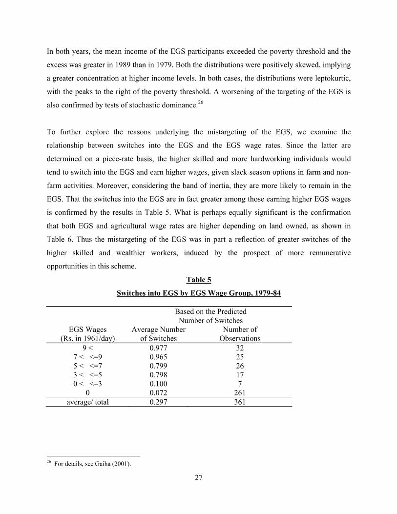
To further explore the reasons underlying the mistargeting of the EGS, we examine the

relationship between switches into the EGS and the EGS wage rates. Since the latter are

determined on a piece-rate basis, the higher skilled and more hardworking individuals would

tend to switch into the EGS and earn higher wages, given slack season options in farm and non-

farm activities. Moreover, considering the band of inertia, they are more likely to remain in the

EGS. That the switches into the EGS are in fact greater among those earning higher EGS wages

is confirmed by the results in Table 5. What is perhaps equally significant is the confirmation

that both EGS and agricultural wage rates are higher depending on land owned, as shown in

Table 6. Thus the mistargeting of the EGS was in part a reflection of greater switches of the

higher skilled and wealthier workers, induced by the prospect of more remunerative

opportunities in this scheme.

Table 5

Switches into EGS by EGS Wage Group, 1979-84 Based on the Predicted Number of Switches

EGS Wages Average Number Number of (Rs. in 1961/day) of Switches Observations

9 < 0.977 32 7 < <=9 0.965 25 5 < <=7 0.799 26 3 < <=5 0.798 17 0 < <=3 0.100 7

0 0.072 261 average/ total 0.297 361

26 For details, see Gaiha (2001).

28

Table 6 Agricultural and EGS Wage Rates by Land Owned, 1979-84

Agricultural Wage Rate

EGS Wage Rate

Owned Area

Mean Wage rate Number of Mean Wage rate Number of (Rs. In 1961/ day) Observations (Rs. In 1961/ day) Observations

10 Acres < 11.41 30 15.00 4 5 < <=10 Acres 10.95 57 9.93 18 2 < <=5 Acres 7.42 128 7.49 35 1 < <=2 Acres 5.99 129 7.12 47 0 < <=1 Acres 5.99 138 5.88 60

0 6.14 386 6.39 166 average/ total 6.78 868 6.81 330

What the preceding analysis suggests is that, while the wage ratio matters, this by itself cannot

explain the worsening of the targeting. The choice between the EGS and regular labour market

activities (in the present context, agriculture) must take into account discounted cash flows

associated with them, the entry and exit costs, and the volatility of agricultural wage rates. The

option value model used here demonstrates how these considerations could be incorporated in a

dynamic optimisation framework. In particular, what emerges from this analysis is that the case

for rural public works is a more complex one, as it must go beyond the screening and deterrent

arguments premised on a fixed wage differential.

5. Concluding Observations

Some observations are made to put the main findings in perspective. A point of departure of this

analysis is the focus on the switches that occur between the EGS- a rural public works scheme

with guaranteed employment at a fixed wage rate- and regular labour market activities with a

market determined stochastic wage rate. As a result, the emphasis is on employment options

judged on the basis of their discounted cash flows. So not just the wages in different activities

but also entry and exit costs matter in labour supply decisions in the option value framework.

The econometric evidence confirms that switches into the EGS are positively linked to the ratio

of EGS/farm wage ratio. It also suggests that switches are linked to variables that proxy some of

29

the entry and exit costs (e.g. employment in the EGS in the previous year). There is also some

evidence confirming greater participation of a top subset of agricultural wage earners in the EGS,

reflecting their ability to better afford higher entry and exit costs. Besides, volatility of

agricultural wage rates matters a great deal. As far as non-farm activities are concerned,

environmental factors reflecting unemployment risks have a more significant role. Taking some

of these factors into account in a dynamic optimisation framework, the analysis suggests that the

selective power of the EGS may be impaired by several biases in favour of higher income

individuals and by the fact that programme entry and exit are not determined by a single income

level but by bands of inertia of different size. An explanation based on these factors may help

understand better the worsening of the targeting of the EGS during the 1980s. But perhaps

equally importantly the fact that switches into the EGS and regular labour market activities are a

result of the joint influence of all these factors suggests that the risk of those benefiting from

public support- especially the poor- becoming dependent on it is considerably exaggerated.

In conclusion, if this analysis has any validity, the incentive case for rural public works schemes

such as the EGS in terms of screening and deterrent arguments needs to be reformulated in a

dynamic optimisation framework, taking into account discounted cash flows, entry and exit costs

and volatility of agricultural wage rates. If an allowance is also made for bands of inertia,

dependent on incomes and individual levels of uncertainty, the incentive case for workfare is

further weakened.

30

Annex: Definitions and Descriptive Statistics of Variables

Variable Name/(Definition): Observations Mean Standard

Deviation CV_wage (Coefficient of Variation of real monthly wage earning) 977 157.91 101.73 CV_wage Ls (CV_wage of Landless) 703 171.37 102.08 Legs_dum (Dummy variable: 1 if one participates in the EGS and 0 Otherwise)

2846 0.12 0.32

Legs_day (Days of participation in the EGS in a crop year: Day) 2846 6.98 27.75 Legs_ern (Earning from the EGS in a crop year: Rs.) 2846 42.07 172.05 L_dumLs (Dummy variable: 1 if the landless participates in the EGS and 0 otherwise)

2271 0.09 0.29

L_dayLs (Days of participation in the EGS in a crop year: positive only in the case of landless: Day)

2271 4.71 21.46

Legs_ern (Earning from the EGS in a crop year, positive only In the case of landless: Rs.)

2271 29.97 140.41

W_ agr (Rreal daily agricultural wage in a crop year) 2846 2.07 4.04 W_ egs (Real daily agricultural wage in a crop year) 2846 0.79 2.49 H_bmi (The BMI index: Weight (in kilograms) devided by height (in metres) squared)

1113 0.19 0.026

H_bmi2 (The square of the BMI index) 1113 0.035 0.0097 School (Years of education: years) 2846 2.48 3.63 A_ age (age: years) 2846 25.19 18.63 A_ female (1 if female and 0 otherwise) 2846 0.48 0.50 A_ high caste (1 if high caste and 0 otherwise) 2846 0.41 0.49 A_ medium high caste (1 if medium high caste and 0 otherwise) 2846 0.25 0.43 A_ medium low caste (1 if medium low caste and 0 otherwise) 2846 0.10 0.30 B _ School (education of household head: years) 2846 2.81 3.87 B _ agri labourer 2) (1 if household head is agricultural labourer and 0 otherwise)

2846 0.28 0.45

B_ debt (household’s debt: Rs.) 2846 3080.87 4705.80 B_ no. of female earner (no. of female earner) 2846 0.72 0.94 B_ no. of male earner (no. of male earner) 2846 1.13 1.37 B_ female household head (whether household head is female) 2846 0.11 0.31

31

B_availability of non-farm employment (total days worked by all household members in non-farm sector)

2846 32.22 86.82

B_ age of household head 2846 48.91 10.50 B_ dependency burden (the share of children under 15 years in a household). 2846 32.08 20.05 V_ land (Land owned by household: Acre) 2846 8.08 14.55 V_ networth (Net- Worth : Total assets of household minus liabilities: Rs.) 2846 13393.28 17451.49 I_ Shirapur (1 if located in Shirapur and 0 otherwise) 2846 0.50 0.500 R _cvrain (CV of rainfall in a year) 2846 59.49 12.87 ε _egs (previous participation in the EGS: days) 2846 29.15 89.64

32

References

Besley, T. and S. Coate (1992) “Workfare versus Welfare: Incentive Arguments for Work-Requirements in Poverty Alleviation Programmes”, The American Economic Review, Vol. 82. Dasgupta, P. (1995) “ Nutritional Status, the Capacity for Work, and Poverty Traps”, London: STICERD, London School of Economics, mimeo. Dev, S. (1993) “India’s (Maharashtra’s) Employment Guarantee Scheme : Lessons from Long Experience”, Bombay : Indira Gandhi Institute of Development Research, mimeo. Dixit, A. K. and R. S. Pindyck (1994) Investment under Uncertainty, Chichester: Princeton University Press. Freund, J. E. and R.E. Walpole (1987) Mathematical Statistics, Fourth edition, New Delhi: Prentice Hall. Gaiha, R. (1997) “Rural Public Works and the Poor: The Case of the Employment Guarantee Scheme in India”, in S. Polachek (ed.) Research in Labour Economics, Vol.16, Conn: JAI Press. Gaiha, R. (2000) “On the Targeting of the Employment Guarantee Scheme in the Indian State of Maharashtra”, Economics of Planning, October. Gaiha, R. (2001) “ Rural Public Works and the Poor- A Review of the Employment Guarantee Scheme in Maharashtra”, Accepted for presentation at the 13th World Congress of the International Economic Association, Lisbon, September, 2002. A revised version was presented at a seminar at Columbia University, November, 2002. Gaiha, R. P.D. Kaushik and Vani Kulkarani (1998) “Jawahar Rozgar Yojana, Panchayats and the Rural Poor in India”, Asian Survey, Vol. XXXVIII. Greene, W. H. (1993) Econometric Analysis, Second edition, New York: Macmillan. Govt. of Maharashtra (GOM, 1997) “Employment Guarantee Scheme”, Mumbai: Planning Department, mimeo. Hirway, I. And P. Terhal (1994) Towards Employment Guarantee in India, New Delhi : Sage Publications. Knudsen, O.K. and P. Scandizzo (2002) An Options Approach to Sustainable Development, Working Paper, World Bank and University of Rome “ Tor Vergata”, mimeo. Ravallion, M. (1991) “Market Responses to Anti-Hunger Policies : Wages, Prices and Employment”, in J. Dreze and A. Sen (eds.) The Political Economy of Hunger, Vol.II, Oxford : Clarendon Press.

33

Ravallion, M., G. Datt and S. Chaudhuri (1993) “Does Maharashtra’s Employment Guarantee Sheme Guarantee Employment? Effects of the 1988 Wage Increase”, Economic Development and Cultural Change, Vol.42. Ravallion, M. and G. Datt (1995) “ Is Targeting through a Work-Requirement Efficient?”, in D. van de Walle and K. Nead (eds.) Public Spending and the Poor, Baltimore: Johns Hopkins University Press. Scandizzo, P., R. Gaiha and K. Imai (2003) Income Stabilisation through the Employment Guarantee Scheme in India, ( in preparation ). Walker, T.S. and J.G. Ryan (1990) Village and Household Economies in India’s Tropics, Baltimore : Johns Hopkins University Press.