Option Exercises, Dilution, and Earnings

Management: Evidence from a Regression

Discontinuity∗

Xing Gao and Mathias Kronlund

University of Illinois at Urbana-Champaign

December 2018

∗A previous draft of this paper was circulated under the title: “Does Dilution from Option Exercises CauseShare Repurchases?”. We thank Heitor Almeida, Alice Bonaime, Felipe Cortes (discussant), Peter Haslag, ScottWeisbenner, Ryan Williams (discussant), Yuhai Xuan and seminar and conference participants at the Universityof Illinois at Urbana-Champaign, NFA Charlevoix, FMA San Diego, and UIC for many helpful comments andsuggestions. Xing Gao is at the University of Illinois at Urbana-Champaign; Department of Economics; 1407 WGregory Dr; Urbana, IL 61801; U.S.A.; Email: hgao12@illinois.edu. Mathias Kronlund is at the Universityof Illinois at Urbana-Champaign; Gies College of Business; 1206 South Sixth Street; Champaign, IL, 61820;U.S.A.; Email: kronlund@illinois.edu

Option Exercises, Dilution, and Earnings

Management: Evidence from a Regression

Discontinuity

December 2018

Abstract

Option exercises increase a firm’s shares outstanding and dilute earnings per share

(EPS), giving the firm an incentive to manage EPS, either by increasing earnings or

through buybacks. We examine what firms do in response to plausibly exogenous option

exercises using a fuzzy regression discontinuity framework, by focusing on close-to-the-

money options near their expiration. If the firm’s share price is just above an option’s

strike price on the expiration date, the option is significantly more likely to be exercised

compared to if the share price ends up just below the strike. We show that these “just-in-

the-money” exercises put pressure on EPS, and firms respond by engaging in both real-

and accruals-based earnings management. These effects are stronger when the exercise is

larger and more dilutive, and hold only when earnings are positive. However, firms do

not engage in more repurchases, suggesting that dilution from options compensation are

not a significant driver of buybacks.

JEL category: 35

Keywords: option exercises, regression discontinuity, earnings management, share repur-

chases, EPS, dilution, executive compensation

1 Introduction

Equity-based compensation for corporate executives, in the form of restricted stock and

stock options, has increased substantially over the last couple of decades. For example, in

2015, CEOs among S&P 1500 firms on average were awarded around $1 million in option

awards (Black-Scholes value), and exercised previously granted options for a value of $3

million. The intended purpose of equity-based pay is to align the interests of managers

and shareholders more closely. Researchers and practitioners have nevertheless recognized

that equity-based pay can have unintended consequences, for example, by encouraging

manipulation of stock prices or by distorting corporate decisions.

This paper investigates one such distortion, namely whether the increase in the firm’s

outstanding shares that results from options compensation can cause firms to manage

their EPS. The basic argument is the following: When executives exercise options, those

options turn into new shares, which causes the number of shares outstanding to expand.

The increased share count mechanically causes per-share performance metrics (such as

EPS) to contract because of the growth in the denominator.1 Analysts and stock market

investors pay careful attention to these per-share metrics, and missing an EPS target,

even if only by a very narrow margin, can disappoint investors and result in negative

stock market returns (Skinner and Sloan, 2002). Furthermore, executives themselves are

often explicitly compensated in the form of bonuses that are tied to meeting or beating

EPS targets, which gives these executives an added incentive to avoid any negative impacts

to EPS. Firms may thus seek to counter the negative effect on EPS that result from option

exercises.

Firms have two main ways of strategically managing EPS: 1) doing a buyback, which

reduces the denominator, or 2) by increasing the earnings (the numerator) through earn-

ings management. Several academic papers have argued that the former mechanism, anti-

dilutive buybacks in response to options compensation, is an important driver of buybacks

(Bens, Nagar, Skinner, and Wong, 2003; Kahle, 2002), and this view is also prevalent in

1The effect from exercises on EPS is bigger for “basic EPS” and relatively smaller for “diluted EPS”,especially for options that are far in the money, because diluted EPS already accounts for the possibility offuture exercises. We will focus on a set of options that are close-to-the-money and thus represent significantshocks to both “basic” and “diluted EPS”.

1

the press, see e.g. (Coggan, 2015). If firms buy back the same number of shares as the

number of options that were exercised, they can perfectly undo the dilution caused by the

exercise and limit the adverse effect on EPS (Coggan, 2015).2 Executives themselves have

also claimed that this channel is important: In a survey of executives, two-thirds of CFOs

cited options anti-dilution as a “very important” or “important” driver of repurchases

(Brav, Graham, Harvey, and Michaely, 2005).

Even though earnings management around option exercises has not received as much

attention, there are nevertheless good reasons to believe that real- and accruals-based

earnings management could be at least as important as repurchases when it comes to

managing EPS around options exercises. For example, in a survey of 400 executives,

Graham, Harvey, and Rajgopal (2005) asked what executives would do if it looked like

their company might come in below the desired EPS target. 80% of executives reported

that they would “decrease discretionary spending (e.g., R&D, advertising, maintenance,

etc.)”, making it the most popular option, and 40% reported they would “book revenues

now rather than next quarter” (i.e., accruals management, making it the third-most

popular option). By contrast, only 12% of executive reported they would repurchase

shares if faced with this situation.

The primary goal of this paper is to employ a novel identification strategy to examine

to what extent firms do share buybacks or engage in other forms of earnings management

strategies to counter the EPS dilution from option exercises. What firms do in about

dilution from options is important. Excessive share buybacks can have real consequences

when the money spent on repurchases instead could have been used to invest in plants,

R&D, or to hire more employees (Almeida, Fos, and Kronlund, 2016). Direct cuts to R&D

and other discretionary spending could, in turn, result in worsened firm performance going

forward (Bens, Nagar, and Wong, 2002, e.g.,).

While previous research has shown that dilution from options and repurchases indeed

2While most buybacks do increase EPS, they do not always do so. Specifically, a repurchase will increase EPSwhen the firm’s earnings-to-price ratio is higher than the opportunity cost of funds (e.g., the after-tax interestearnings on cash holdings or the marginal cost of debt used to pay for the buyback). As an obvious example,a firm with negative earnings would only cause its EPS to become even more negative if doing a buyback toreduce the number of shares.

2

are strongly correlated (Bens et al., 2003; Kahle, 2002, e.g.,), it is naturally challenging

to establish whether options have a causal impact on repurchases as implied by the “anti-

dilution” hypothesis. The reason is that both the extent to which executives receive

options, when and whether those options are dilutive or end up being exercised, as well as

the extent of share buybacks are endogenous outcomes that depend on multiple industry-,

firm-, and executive-level factors that are difficult to control for in a regression framework.

Options can also put pressure on diluted EPS even before they are exercised, raising the

question whether firms should manage “basic” or “diluted” EPS.3 For outstanding options

to have a significant impact on diluted EPS, that implies that the firm in the past has

awarded many options and also that the firm’s stock price has performed well since then,

so that the options are now (far) in-the-money. A wide range of firm characteristics,

including recent firm performance, growth opportunities, life cycle, and liquidity position

can affect both a firm’s use of options compensation and its payout policy. These kinds of

factors could plausibly introduce a spurious correlation between exercises and repurchases,

in which case their relationship may not be causal.4

Consider a firm that has experienced strong returns—that firm is more likely to ex-

perience exercises because its options are more likely to be in-the-money, but strong

stock performance often goes hand-in-hand with high cash flows that the firm can use for

buybacks. Similarly, younger firms are more likely to use stock options as part of their

compensation packages because they are “cash-poor”; but these firms may also not want

to commit to regular dividend payments but instead use repurchases to distribute any

excess cash. Causal inference in this setting is challenging precisely because factors like a

firm’s life cycle and financial constraints can be hard to measure well and perfectly control

for in a regression framework (see, for example, Erickson and Whited (2000). The direc-

tion of causality could even go the other way, from repurchases to options: for example,

3The effect of outstanding but yet-unexercised options on diluted EPS—based on the “treasury stockmethod”—is calculated by assuming that any cash the firm receives as the strike price in the exercise would beused to buy back shares. The resulting formula for the “impact” of each option is max{0, 1-X/P}, where X isthe strike price and P is the firm’s share price. The treasury stock method thus implies that, for example, ifa firm has 1000 outstanding options with a strike price of $25 and a share price of $50, the number of sharesthat are added to current shares when calculating diluted EPS is 500 (1000*(1-25/50)). Conversely, outstandingoptions that are out-of-the-money or at-the-money do not affect diluted EPS.

4Larcker (2003) makes this argument in a concurrent comment on Bens et al. (2003).

3

Babenko (2009) show that buybacks increase employees’ pay-performance sensitivity and

cause employees to carry more risk, which in turn encourages employees to exercise their

options.

To examine the causal effect of exercises on EPS management (share repurchases and

earnings management), this paper employs a “fuzzy regression discontinuity” (fuzzy RD)

framework. The idea behind the experiment we have in mind is the following: Imagine

two firms, A and B, that both awarded their executives 100,000 options in 2006 that are

set to expire in 2016; both firms’ stock prices on the grant date were $25, and as is typical

for executive options, the strike price for these options was the same as the stock price

when they were granted (i.e., “at-the-money”). Fast-forward to 2016 when these options

are about to expire; now, suppose the stock prices of these firms have been fairly stagnant,

and so their stock prices remain around $25. Firm A has nevertheless performed slightly

better than firm B: Firm A has a stock price of $25.50, while firm B has a stock price of

$24.50 on the day when the options are about to expire. Despite similar characteristics

and almost-identical performance, the executives in firm A are more likely to exercise

their options which would increase the number of shares outstanding, compared to firm

B. This framework thus provides a quasi-exogenous shock to exercises, and according to

the anti-dilution hypothesis, we might then expect firm A to buy back shares or engage in

other forms of earnings management in response to these exercises to maintain its EPS,

compared to firm B that experiences no dilution. One prominent example of this kind of

situation involves Goldman Sachs CEO Lloyd Blankfein and Bank of America CEO Brian

Moynihan, both of whom received around 200,000 options in late 2006 and early 2007.

Goldman’s stock price was almost perfectly flat over the 10-year period after Blankfein’s

options were granted, but narrowly rose above the strike price (by around 2%) by the

time the options were about to expire, causing Blankfein to exercise his options, whereas

Moynihan’s options expired worthless.5

In our empirical framework, we first define the variable price gap as the difference on

the option expiration date between the firm’s share price and the option’s strike price

5See the Wall Street Journal (Feb 16, 2017) at https://www.wsj.com/articles/bank-of-america-misses-a-big-options-payday-goldman-cashes-in-1487154601

4

(adjusted for splits and stock dividends since the grant), normalized by the adjusted

strike price. In the example above, this was $0.5/25=+2% for firm A and $-0.50/25=-2%

for firm B, respectively. At a price gap of zero, there is a discrete jump in the level of

exercises, where executives with options to the right of the gap are more likely to exercise

their options because they end up slightly in-the-money. We then limit the observations

to only instances of price gaps that fall within a narrow price gap window of 20% around

the strike price and examine how the discontinuity around the zero-price-gap relates to

changes in firm outcomes (while controlling for any linear relation with the price gap).6

The RD is “fuzzy” (Angrist and Lavy, 1999; Van der Klaauw, 2002), because a stock

price above the strike price on the expiration date does not guarantee that the option

is exercised and that no options are exercised below, but it nevertheless increases the

likelihood that an option is exercised.

There are several reasons why the price gap does not produce a “sharp” discontinuity.

First, options can be forfeited or re-structured throughout an option’s life (usually 10

years), for example, if an executive leaves the firm or if there is a reorganization such

as an acquisition or a merger. Second, even though most options have vesting require-

ments that require executives to continue holding an option for several years, an option

can be exercised early anytime after the vesting period, and many executives do exercise

early (Klein and Maug, 2011). Theoretically, a risk-neutral executive should never exer-

cise a call option early except possibly before a dividend payment (Merton, 1973), and

even risk-averse executives should not exercise early unless the option is far in-the-money

(Carpenter, Stanton, and Wallace, 2010). In our setting, early exercises are less common,

precisely because the options that we focus on are by construction out of the money or

only barely in the money for most of their lives. Third, executives sometimes exercise

options even if they are slightly out-of-the-money, i.e. when the price gap is negative (Fos

and Jiang, 2015). The fact that we do not have a sharp discontinuity for many of these

reasons is not a threat to the validity of the identification strategy, but it nevertheless

affects how we should interpret the resulting regression coefficients. Specifically, the re-

sults from the fuzzy RD are a local average treatment effect (LATE) which captures the

6Our results are robust to alternative definitions of the bandwidth around the threshold.

5

effect among firms where the executive’s decision to exercise or not depends on whether

the price is above or below the strike price on expiration (“compliers”). We nevertheless

do require that at least some executives hold their options until close to the expiration

for there to be a statistically strong “first stage”, so that the likelihood that an option is

exercised indeed increases discontinuously around the zero-price-gap threshold.

Our data starts with all executive options in the Execucomp database that have been

granted after 1992 and that also expired by the end of 2016. Every firm has several

executives, all of whom in turn can hold several options, but our primary outcome variables

are defined at the firm-quarter level, which implies that we need to carefully aggregate our

data across options to get a firm-quarter level measure of the price gap. To do so, if a firm

has multiple options that have the same expiration day and strike price, we treat them

as one but sum across the number of shares that underlie the options. We further drop

options that have been fully exercised before the quarter when the option expires, or if

the still-unexercised size is smaller than 0.1% of shares outstanding. If a firm has multiple

options that expire in the same quarter, but with different strike prices or expiration dates,

we further select only the largest option. This process results in a total of 5,183 options

that are unique to a firm-quarter. When we limit the sample to only those options that

fall within the 20% price gap range, we end up with 899 options, which makes up the core

of our sample. These options on average represent around 0.4% of shares outstanding.

This magnitude is similar to the level of quarterly repurchases—which means that if these

options were to be offset by repurchases that would in turn represent a sizeable shock to

buyback activity.

In our empirical analysis, we start by showing that the first stage—i.e., the relation

between the zero-price-gap threshold and exercises—is strong. When we plot exercises on

the price gap on the expiration date (Figure 1), we see that there is a discontinuity in

the level of exercises right around the zero-threshold. There are very few exercises to the

left of the threshold and many exercises to the right of the threshold.7 Importantly, the

7We also observe that there are some exercises also in the price gap region between -2% and 0. This isconsistent with the “out-of-the-money” exercises studied by Fos and Jiang (2015) and Jensen and Pedersen(2016). Another reason for observing exercises with a negative price gap is that these exercises could have beendone a few days or hours before the close on the expiration date when the price gap might have still been positive,

6

strength of the first stage is stronger when the underlying option is large. We further show

that the higher level of exercises results in an increase in the number of shares outstanding

and a mechanical decrease in EPS due to the increase in the denominator.

If firms seek to counter the dilutive effect of these plausibly exogenous option exercises,

we should then observe more repurchases and/or more earnings management just to the

right of the zero-price-gap threshold compared to the left. On the other hand, it is also

possible that firms do not respond to these exercises—for example, if managers count on

investors and analysts realizing that any negative effect on EPS was purely “mechanical”—

in which case we would not observe any jump in repurchases or earnings management

around the threshold. Crucially, the positive price gap indicator is plausibly uncorrelated

with the many other reasons firms may have to engage in earnings management or share

buybacks—which is one of the main advantages of this empirical strategy.8

Contrary to a positive relation between option exercises and repurchases, we show that

firms do not engage in increased share buybacks in response to these quasi-exogenous

exercises. Firms on either side of the zero-price-gap threshold have remarkably similar

repurchase patterns, both repurchasing around 0.6% of total assets. This is true even

for the largest options, which represent the greatest shock to shares outstanding, and

also among firms that explicitly compensate their managers based on EPS and may have

the strongest incentive to respond. We also see no delayed response over the following

quarter or year, suggesting that the firms that experience exercises do not buy back the

newly issued shares even with a delay. In sum, these results suggest that share dilution

from exercises is not a significant causal driver of share repurchases. Firms thus appear

willing to tolerate the resulting share expansion and not significantly alter buyback plans

in response.

but that the stock price subsequently drifted down to end up with a negative price gap. Such mismeasurementaround the threshold has the potential to shrink our regression coefficients but is small enough that it doesnot affect the first stage significantly. However, as an added robustness test, we also estimate our results usinga “Donut RD” strategy which throws out the observations in a region of 1% around the threshold; see, e.g.,Almond and Doyle (2011); Cahuc, Carcillo, and Le Barbanchon (2014); Rau, Sarzosa, and Urzua (2015) forother examples of Donut RD.

8For example, common reasons for buybacks include tax-efficiency (Desai and Jin, 2011), optimal leverage(Bagwell and Shoven, 1989), undervaluation (Ikenberry, Lakonishok, and Vermaelen, 1995), agency problems(Jensen, 1986), liquidity (Cook, Krigman, and Leach, 2003; Hillert, Maug, and Obernberger, 2016), or fendingoff takeovers (Bagwell, 1991; Billett and Xue, 2007).

7

Instead, we show that firms strongly engage in earnings management around these

exercises. This happens both in the form of reduced R&D spending and higher accruals.

These effects are stronger and only significant for firms that have positive earnings—firms

with negative earnings naturally have no incentive to manage earnings around option ex-

ercises, since an expansion in shares makes their EPS better. We also show that especially

accruals management is much stronger for firms where managers are explicitly compen-

sated based on EPS. As a result of this earnings management, even though we observe a

“mechanical” decrease in EPS that’s driven by the denominator, the firms to the right of

the threshold actually report higher increases in EPS because of higher growth in earnings

(the numerator) compared to the firms on the left of the threshold. In sum, our results

show that firms manage earnings when faced with a need to counter adverse shocks to

EPS, but that repurchases are not affected.

We conduct several robustness tests to support the assumptions behind the quasi-

experimental RD design. One possible threat to the identification could arise if firms

manipulate the share price around exercises. Previous studies have shown that managers

manage share prices around option grants (Baker, Collins, and Reitenga, 2003; Chauvin

and Shenoy, 2001; Yermack, 1997, e.g.,), although there is less evidence of manipulation

around option exercises (Carpenter and Remmers, 2001). Intuitively, executives do not

have a particularly strong incentive to manage the share price precisely around the price

gap threshold, because if the firm ends up just narrowly to the right of the price gap,

then executives profit only based on the small difference between the strike price and the

share price. In other words, the payoff from options as a function of the share price is

continuous and exhibits no discrete jumps. Furthermore, to pose a threat to the identifica-

tion strategy, it would have to be that managers to the right of the threshold manipulate

differently from managers on the left, which is even harder to believe. Nevertheless, if

managers do manipulate share prices so that they end up just-in-the-money, we would

expect to see a mass of observations to the right of the threshold. We formally investigate

this possibility but observe no “bunching” on either side of the threshold, but firms are

smoothly distributed around the zero price gap threshold, which is thus consistent with

“non-manipulation” of the assignment variable. Further, there are no systematic differ-

8

ences in other observable characteristics of the firms that end up on either side of the

threshold. We also examine possible pre-trends and show that the firms that end up on

the left and the right were also on similar trends before the expiration quarter. These

tests thus support the notion that it is truly random which firms ended up on the right

side of the threshold and which firms ended up on the left.

Our paper proceeds as follows. The next section describes the related literature. Sec-

tion 3 describes our data and measurement. Section 4 presents summary statistics. Section

5 describes the results from OLS correlations, and Section 6 describes the fuzzy RD em-

pirical strategy and the first-stage results on exercises. Section 7 presents results for firm

responses to exercises. Section 8 discusses robustness tests, and Section 9 concludes the

paper.

2 Literature

This paper relates to the literature that links executive compensation—and specifically

exercises—to payout decisions. Weisbenner (2000), Kahle (2002), Bens et al. (2003) were

among the first to study the relation between options compensation and payout policy.

A more recent paper is by Ferri and Li (2016) who consider the relation between options

compensation and payout policy using a diff-in-diff design. Ferri and Li (2016) specifi-

cally exploit a change to accounting standards (FAS123R) that mandated option grants

to be expensed, which has been followed by firms awarding fewer options. They find

that firms that were most “exposed” to FAS123R (the firms that had previously awarded

the most options) did not change their dividends or buybacks after the law compared to

other firms. Their question is slightly different from ours, as they focus on the effect of

option grants on payout policy, and thus do not directly consider whether the channel

between repurchases and options goes through dilution. Option grants can importantly

affect payout policy even independent of dilution because dividend payments decrease the

value of options, which can encourage firms to substitute repurchases for dividends—a

“dividend-substitution hypothesis” (Fenn and Liang, 2001; Kahle, 2002; Lambert, Lanen,

and Larcker, 1989; Liljeblom and Pasternack, 2006). Our empirical strategy instead ex-

9

plicitly tests the “anti-dilution hypothesis” under which repurchases are driven by dilution

and exercises but not directly by grants; if options were granted but did not end up in-

the-money, there would be no dilution. In contrast, under the “dividend-substitution”

hypothesis, the grants themselves cause firms to substitute away from dividends, and that

incentive is not related to whether the options end up being exercised or not.

This paper also relates to the literature that studies the link between repurchases

and earnings management. Hribar, Jenkins, and Johnson (2006) and Almeida, Fos, and

Kronlund (2016) document an abnormally high number of EPS-increasing repurchases

among firms that otherwise would have small negative earnings surprises. Almeida et al.

(2016) further show that this effect is particularly strong for firms that use EPS as an

incentive measure for executives. Cheng, Harford, and Zhang (2015) also find that firms

are more likely to do repurchases if executives’ incentive plans are tied to earnings per

share. In contrast to this literature, we find that in the setting of EPS dilution due to

exercises, firms do not use repurchases as a tool to manage EPS. We find that firms instead

are more likely to use earnings management when faced with adverse shocks to EPS from

exercises, which is consistent. Bergstresser and Philippon (2006) also show a correlation

between option exercises and high accruals, although their story behind this association

is one of opportunistic (i.e., endogenous) exercises in times when accruals are high, and

not of earnings management as a response to dilution. In contrast to Bergstresser and

Philippon (2006), we thus show that there is a causal link that also goes from (exogenous)

exercises to earnings management.

Other papers have studied the relation between options and other corporate policies

such as investment. Chava and Purnanandam (2010) find that executives with risk-

increasing incentives adopt riskier corporate policies, such as higher leverage, lower cash

holdings, and shorter debt maturities. Babenko, Lemmon, and Tserlukevich (2011) show

that an increase in cash flows to the firm from exercises can increase real investment,

especially for firms with high external financing costs. The empirical setting that Babenko

et al. (2011) employ is most similar to ours as they proxy for the level of exercises using the

ratio of the end-of-year stock price divided by average strike price for outstanding options

(across all employees in a firm). They show that as employee options “on average” are

10

more in the money, we observe more exercises. The main difference in the empirical setup

between Babenko et al. (2011) and this paper is that because Babenko et al. average

across a lot of different options for all executive and non-executive employees (who may

have received their options at different times with different strike prices, and which may

not be exercisable), they do not observe any jumps in the likelihood of exercises as a

function of the “price ratio” they use. Their identification instead principally relies on

changes in the slope of exercise intensity over a wide domain of the ratio.

3 Data and Measurement

3.1 Measuring Options

We collect data on options that were awarded starting from 1992 and that expired be-

fore the end of 2016. Our data source for option grant data is Compustat’s Execucomp

database. Because the SEC changed the disclosure requirements and reporting format of

option grants in 2006, we employ two different tables from Execucomp before and after

the disclosure reform.9 For options that expire from 2007 onwards, we use the “Plan-

Based Awards” table, which lists both new options granted in a fiscal year as well as the

previously-granted-and-still-outstanding options as of the fiscal year-end. Because options

are listed in this table every year between the grant year until the option disappears, we

limit the observations to options that are scheduled to expire during the upcoming fiscal

year. Filtering the sample of options in this manner eliminates any duplicate observations

from the same option being listed across multiple years, and also by construction elimi-

nates any options that have been forfeited, restructured, or exercised early before the start

of the last fiscal year of the option’s life. For options that expire before 2007 and thus are

not covered by the “Plan-Based Awards” table, we instead use the “Stock Option Grants

Awards” table. Because most options have a 10-year life, this mostly includes options

that were granted between 1992 and 1996. The “Stock Option Grants Awards” table lists

all options as of the year when they are granted. Because we cannot directly filter the

9See the SEC’s final rule on “executive compensation and related person disclosure” at:https://www.sec.gov/rules/final/2006/33-8732a.pdf

11

options from this table based on whether these options are still “live” as of the last fiscal

year before the option expires, we expect the first stage for this subset of options to be

slightly weaker compared to the observations from the “Plan-Based Awards” table.

For each option, we get data on the number of underlying shares, the grant date,

expiration date, and strike price. Our identification strategy compares firms with options

that end up narrowly in-the-money and thus are more likely to be exercised versus firms

with options that expire out-of-the-money. To measure whether an option is in-the-money

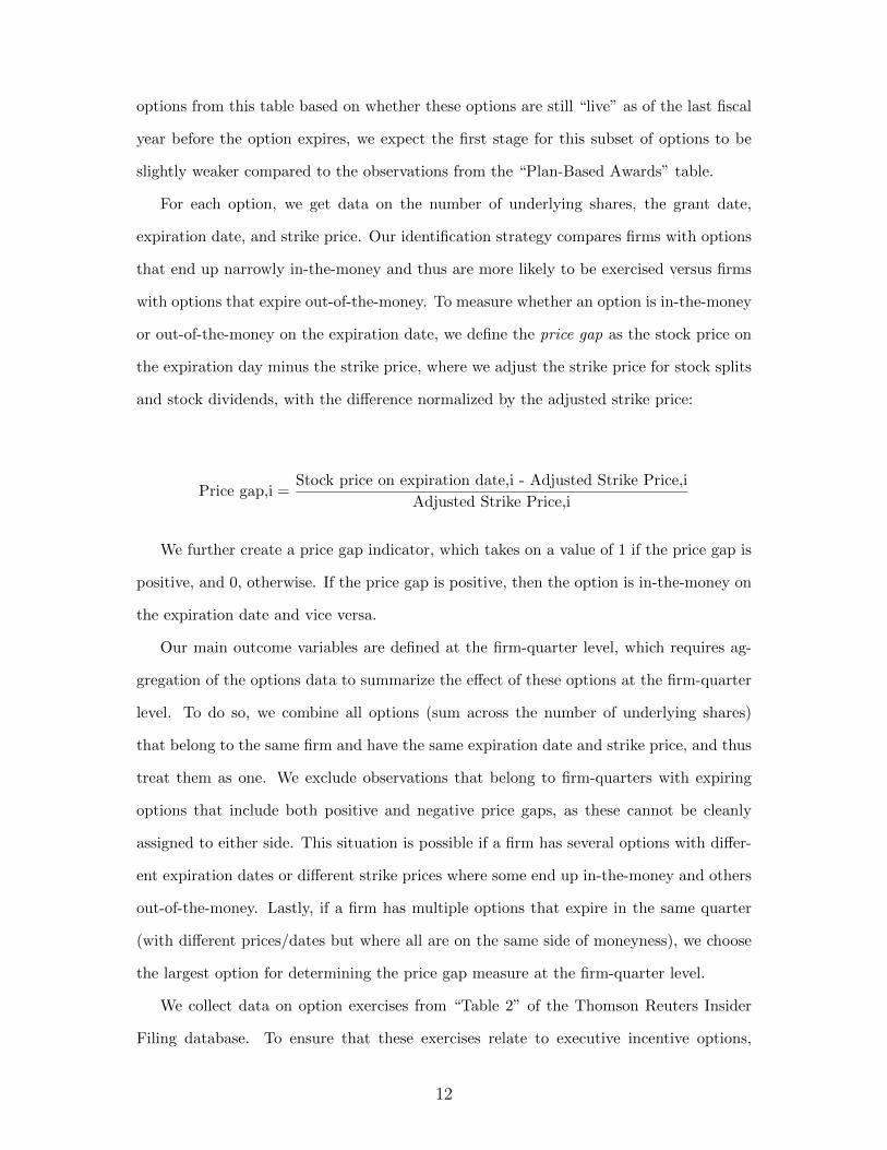
or out-of-the-money on the expiration date, we define the price gap as the stock price on

the expiration day minus the strike price, where we adjust the strike price for stock splits

and stock dividends, with the difference normalized by the adjusted strike price:

Price gap,i =Stock price on expiration date,i - Adjusted Strike Price,i

Adjusted Strike Price,i

We further create a price gap indicator, which takes on a value of 1 if the price gap is

positive, and 0, otherwise. If the price gap is positive, then the option is in-the-money on

the expiration date and vice versa.

Our main outcome variables are defined at the firm-quarter level, which requires ag-

gregation of the options data to summarize the effect of these options at the firm-quarter

level. To do so, we combine all options (sum across the number of underlying shares)

that belong to the same firm and have the same expiration date and strike price, and thus

treat them as one. We exclude observations that belong to firm-quarters with expiring

options that include both positive and negative price gaps, as these cannot be cleanly

assigned to either side. This situation is possible if a firm has several options with differ-

ent expiration dates or different strike prices where some end up in-the-money and others

out-of-the-money. Lastly, if a firm has multiple options that expire in the same quarter

(with different prices/dates but where all are on the same side of moneyness), we choose

the largest option for determining the price gap measure at the firm-quarter level.

We collect data on option exercises from “Table 2” of the Thomson Reuters Insider

Filing database. To ensure that these exercises relate to executive incentive options,

12

we first limit this data to filings that are reported on Form 4 (“change in an insider’s

ownership position”) with the transaction code “M” (exercises of derivative securities).

We further restrict the reported derivative “type” to be either options, employee stock

option, non-qualified stock option, call option, or incentive stock option, and we drop

observations with a cleanse code that indicates invalid or missing data elements.10

To attain a more accurate representation of the expected size of the potential dilutive

impact of an option as it gets close to expiration, we subtract from each option’s reported

size (from Execucomp) the number of options that have already been exercised up until

the start of the last quarter of the option’s life. To do so, we use the Thomson database

and calculate the cumulative split-adjusted number of exercised options for each option

award (where we match awards between the databases based on cusip, strike price, and

the expiration date) up until the start of the quarter of expiration. We then define the

option size as the reported size from Execucomp minus the cumulative number of options

that have been already exercised. We use these exercises to drop any options that we

know have been fully exercised, or if the still-unexercised size is less than 0.1% of share

outstanding.

Because we require detailed option-level data on the strike price and expiration date of

each option, we focus by necessity on only the options of only the “named executive offi-

cers”, for whom options grants are detailed in SEC filings. Some of the previous research

also has considered options belonging to non-executive employees, including Kahle (2002),

Bens et al. (2003), and Babenko et al. (2011). The problem for our purposes of using all

employee option data is that the only information available from firm filings are average

strike prices and the total number of options, but not individual option-level data. If

detailed option-level data on employee-level options were available, we would clearly like

to include them as well. However this is not a significant threat to our study for at least

two reasons: First, both executive options and employee options should have the same

effect, since they equally cause dilution, so we have no reason to believe that a firm’s

reaction to employee exercises would result in a different effect from how firms react to

10We may inadvertently undercount actual exercises, both due to imperfect merging between Thomson andExecucomp and in applying the previously mentioned filters—this in turn can make the first stage appearrelatively smaller in magnitude than the true level of exercises.

13

executive options. Second, even though non-executive options can make up a significant

part of the total option pool, each option is often individually smaller, which means that

these options may commonly not clear the 0.1% (as a fraction of shares outstanding) size

hurdle we require for inclusion in our sample.

Finally, the previous literature has debated whether firms should be more worried

about managing basic vs. diluted EPS, and thus whether they should manage EPS the

moment an option becomes dilutive for diluted EPS (which can happen gradually as an

outstanding option gets farther into the money) or when an option is exercised and causes

dilution to basic EPS (Bens et al., 2003, see, e.g.). Our setting of examining close-to-

the-money options is ideal for tackling the timing question of whether to manage dilution

before the actual exercise or not, because the options that we study have almost no dilution

before they are exercised, and become 100% (or 0%) dilutive after they are exercised (if

the option ends up in the money) or expire. For example, an option that is 10% in the

money would be 9% dilutive (1-X/P, according to the treasury stock method,) right before

it is exercised, but jumps to being 100% dilutive the moment it is exercised. So even if a

firm has bought back some shares before exercise, there is a big shock to the incentive to

manage both basic and diluted EPS right at the time of exercise.

3.2 Measuring Repurchases, Earnings Management, and other

Outcome Variables

We merge the firm-quarter level options data on the price gap with stock-level data from

CRSP and firm-level data from the Compustat Quarterly file. We drop observations for

firms with a stock price of less than one dollar or assets less than $1 million. The full

merged sample consists of 5,183 observations that are unique to a firm-quarter. Of these,

899 represent firm-quarters where the absolute price gap is within 20%.

We measure repurchases using Compustat’s variable “purchases of common and pre-

ferred stocks” minus any decrease in the par value of preferred stock, normalized by lagged

total assets. This is different from the common way of measuring repurchases as a change

in treasury shares, or as the difference between purchases and sales of stock (Fama and

14

French, 2001). The reason for why we measure repurchases this way is that we do not want

to measure repurchases based on changes in treasury shares, because this measure can be

mechanically confounded by exercises. For example, suppose an executive exercised an

option and was awarded stock from the company’s treasury shares, thus decreasing the

treasury shares, and the firm subsequently repurchased the same number of shares, adding

to the treasury stock. In this case, the firm has repurchased shares to undo the dilution

from options perfectly, but we would not be able to detect that buyback based on the

change in treasury shares which was zero. We do not subtract sales of shares from pur-

chases because we want to isolate gross buyback activity. Banyi, Dyl, and Kahle (2005)

compare reported repurchases from annual filings with measures available in Compustat,

and conclude that the measure of repurchases that we use is the most accurate measure of

actual repurchases, especially for firms using stock options, because it is not mechanically

affected by equity issuance and the exercise of options.

To measure earnings management, we focus on two different kinds of earnings man-

agement: real and accruals-based. For real earnings management, we consider reductions

in spending on R&D. R&D is a form of discretionary spending that is one of the most

commonly used measures of real earnings management (Baber, Fairfield, and Haggard,

1991; Bushee, 1998; Dechow and Sloan, 1991; Roychowdhury, 2006, see, for example); for

example, Baber et al. (1991) show that firms spend less on R&D when they are worried

about meeting earnings targets. For accruals-based earnings management, we use three

different measures that are based on total accruals as well as two different measures of

discretionary accruals, following the Jones model (Dechow, Sloan, and Sweeney, 1995),

respectively. As is common in the earnings management literature, we focus on absolute

accruals (Bergstresser and Philippon, 2006; Cohen, Dey, and Lys, 2008; Cornett, Marcus,

and Tehranian, 2008). For our first measure of discretionary accruals, we calculate residu-

als from regressing total accruals on the inverse of lagged assets, sales growth, and PP&E,

all scaled by lagged assets (Bergstresser and Philippon, 2006, for a detailed example, see,

e.g.,). For the second measure of discretionary accruals, we further adjust each these ac-

cruals by the average level of accruals across all firms in that quarter for a “time-adjusted”

measure. Finally, we use data from IncentiveLab on whether an executive’s compensation

15

is explicitly tied to EPS. Definitions of these variables are found in the data appendix.

All variables are winsorized at the 1% level.

4 Summary statistics

Table 1 presents summary statistics for options (panel A), exercises and payout variables

(panel B), other outcome variables (panel C), and control variables (panel D). In Column

1, we present summary statistics for all observations, and in Columns 2 and 3, we present

statistics for observations that have a positive versus negative price gap. In Columns 4–6,

we further limit this to observations with a price gap between -20% and 20%; in other

words, where the stock price on the expiration date falls within 20% of the strike price.

Column 7 presents t-tests for the difference between Columns 5 and 6.

[Insert Table 1 about here]

Panel A in Table 1 reports summary statistics for option-level statistics such as the

stock price on the expiration day, strike price, price gap, and option size. The average

price gap is 0.969 on average (Column 1), which implies that a typical option ends up far

in-the-money on expiration, although this distribution is right-skewed (the median price

gap is 0.16). Out of the 5,183 options in our sample, 2,917 end up with a positive price gap

while 2,266 options end up with a negative price gap. The average option size represents

0.48% of shares outstanding. When we limit the sample to the 899 options within the 20%

range around the zero-price-gap, we observe that the average price gaps in the “positive”

(Column 5) versus “negative” (Column 6) groups are 0.094 and -0.107 respectively, as we

would expect if these options are distributed relatively evenly in the 20% range around

the strike price. Overall, the options that end up with a negative or positive price gap

look similar based on their strike price and size, though of course the options with positive

price gaps on average have a slightly higher stock price on expiration.

Panel B reports statistics on exercises and payout policy in the quarter when an option

16

expires (we refer to this quarter as “q0”). Comparing exercises for firm-quarters that

have positive (Column 2) versus negative (Column 3) price gaps, we find that there are

significantly more exercises for firms that experience a positive price gap. The probability

of having an option exercise is 43% for observations with a positive price gap, and 5%

for negative price gaps. On average, firms tend to repurchase 0.62% of total assets in a

quarter.11 Comparing Columns 2 and 3, we observe that options that are in-the-money at

expiration tend to belong to firms that have higher payouts than those with options with

negative price gaps, which is natural because the firms with positive price gaps have clearly

performed better, and thus motivates why doing looking at the regression discontinuity is

important. In columns (5)–(6), where we limit the sample to only observations within the

narrow price gap, payouts appear more balanced across the groups with a positive versus

negative price gaps: Both groups of firms repurchase around 0.6–0.61% of total assets in

the quarter of expiration. These simple statistics offer a first hint at our finding in Section

7 that firms do not respond to exercises by repurchasing shares: If these firms did perfect

anti-dilution of the options, we would expect to the positive-price-gap firms to display

significantly more buybacks. That said, while these simple averages compare all firms

within the relatively narrow band, the regression discontinuity design enables us to more

precisely determine whether there is a discrete jump precisely around the zero-price-gap

threshold while controlling for any possible linear relation between the price gap and our

outcome variables.

Panel C reports changes in other variables from q−1 (the quarter before expiration)

to q0, including changes in shares outstanding, measures of EPS, earnings management,

shares issued, and cash balances. Comparing Columns 5 and 6 in Panel C, we observe that

outstanding shares increase more (by around double) for firms with positive compared to

negative price gaps, thus mechanically putting pressure on EPS, although the difference in

11For comparison to other research on buybacks, note that these figures are not the unconditional averagein Compustat for the sample period, but rather the average conditional on having an expiring option in thatquarter, as that is required for the price gap variable to be defined. In Table A1 in the Appendix, we also reportsimilar statistics for all firms in Compustat, over the same period, regardless of whether they have outstandingoptions or not. Comparing these statistics to those of Panel B of Table 1, we observe that firms that use optionson average tend to engage in more share repurchases compared to the average firm in Compustat, with thecaveat that such comparisons are likely confounded by omitted variables.

17

this simple comparison of means is not statistically significant at conventional levels. Of

particular note is our measure the “mechanical” denominator-driven EPS change, which

is defined as lagged earnings divided by current shares outstanding minus lagged earnings

divided by lagged shares outstanding; i.e., this measure captures the change in EPS that

would be expected if the numerator does not change, and we show that the firms on

the positive side exhibit more downward denominator-driven pressure on EPS compared

to their peers with slightly negative price gaps. However, Panel C also shows that the

changes to reported diluted and basic EPS, despite the increase in the number of shares,

are higher for the firms with a positive price gap, indicating that these firms also grow

their earnings even more. While these are only suggestive summary statistics, we formally

test these outcome variables within the fuzzy RD framework in Section 7.

We observe that firms with slightly positive price gaps have a larger increase in cash

and shares issued than firms with slightly negative price gaps, consistent with cash in-

flows from exercises and new issues of shares in exchange, although these differences are

not statistically significant in the simple comparison of means. It is important to note

that employees who exercise options often have access to “cash-less exercises”, where the

employee does not have to put up money for the exercise price, but merely receives the

difference between the strike price and share price, either in the form of cash or shares.

However, even in these cases, the effect on the firm is the same—the firm receives money

for the strike price and issues shares, but a broker or bank is acting as an intermediary

by making a loan to the employee for the exercise price and immediately selling some of

the shares received in exchange to pay back the loan (Heath, Huddart, and Lang, 1999).

Finally, Panel D of Table 1 presents statistics for several firm-level control variables,

including market-to-book, cash flow, cash holdings, ROA, debt-to-assets, firm size, and

an EPS incentive indicator. These variables are measured as of the end of the previous

quarter (most variables), or as of the end of last fiscal year (in the case of the EPS

indicator) before the expiration quarter. Importantly, when we narrow the window to a

range of 20% around the zero-price-gap, the characteristics across the positive and negative

groups appear balanced, and any differences are statistically insignificant. These findings

support the identification assumption that the firms that narrowly end up on either side

18

of the threshold are observationally equivalent when it comes to possible confounders to

our empirical strategy.

5 Motivating correlational evidence

Before moving on to our regression discontinuity results, we also confirm the evidence in

the current literature that there is a strong correlation between repurchases and options

compensation, regardless of whether we measure options compensation using the amount

of option grants, the amount of exercises, or the amount of unexercised exercisable options.

Table 2 tests this hypothesis using OLS regressions over the period 1992–2017. We regress

the log value of quarterly repurchases as the dependent variable on the log value of options

grants, the log value of unexercised exercisable options, and the log value of exercises using

firm-year level data from Compustat and Execucomp.

[Insert Table 2 about here]

The results in Panel of Table 2 show that repurchases are indeed strongly correlated

with the value of option grants, option exercises, and exercisable options, both separately

and when including all of these independent variables simultaneously. We further control

for possible measurable confounders such as firm age and size, as well as industry × year

fixed effects, with broadly similar results albeit smaller coefficients. These correlations also

continue to hold after controlling for firm fixed effects which means that the same firm

tends to do more repurchases during times when many options are granted, exercisable,

or exercised, even though the economic coefficients here become yet smaller.

On the one hand, this evidence is consistent with a hypothesis of anti-dilution moti-

vated repurchases. On the other hand, both repurchases and exercises could be driven

by some unmeasured omitted factor such as financial constraints or performance, which

makes a causal relationship challenging to ascertain. In addition to the measurable char-

acteristics we control for, there are likely also many unobservable characteristics that differ

19

across firms that affect both buybacks and options. The simple control variables that we

employ in Table 2 reduce the estimated coefficients on exercised/exercisable options to

almost a quarter of the original magnitude (from around 0.18 to 0.05). The omitted vari-

able concern then is that it is plausible that a few still-omitted or hard-to-measure control

variables, such as firm lifecycle or investment opportunities, could plausibly explain any

remaining association between repurchases and options.

One way to ask whether the regression evidence of a relation between repurchases

and option exercise is evidence of anti-dilutive buybacks is to test this in a sample where

it should not work. Panel B of Table 2 therefore restricts the sample to firm-quarter

observations with negative income. If anti-dilution from option exercises is a reason behind

repurchases, firms should not be more likely to conduct repurchases in response to option

exercises when their income is negative. However, if the positive correlation between

repurchases and option awards is driven by other omitted variables, we may still observe

a positive relationship between repurchases and option awards even during times with

negative income. We find that in the sample of only quarters with negative income, the

coefficients of option exercise and unexercised exercisable options are still significantly

positive. This finding provides suggestive evidence that the relationship may not be

causal or driven by earnings management concerns, thus further motivating the empirical

strategy that we describe in the next section.

6 Empirical strategy and first stage results

To examine whether a causal relationship exists between option exercises and the various

methods of managing EPS, we need an identification strategy that allows for plausibly

exogenous variation in exercises that can isolate the effect of these exercises. We employ

a fuzzy RD strategy (Angrist and Lavy, 1999; Van der Klaauw, 2002), by focusing on

options that expire with a stock price close to the strike price. While firms that fall

narrowly on either side of the zero-price-gap are ex-ante similar (as was shown in Panel

D of Table 1), when a firm ends up on the positive side the option expires in-the-money

20

and is therefore more likely be exercised, while on the negative side the options will more

likely expire out-of-the-money.

To illustrate the discontinuous effect on exercises that is caused by the price gap,

Figure 1 plots firm-quarter-level exercises of expiring options on bins of price gap on

expiration (i.e., the “first stage”). The x-axis represents normalized price gaps falling

in the range of -0.2 to 0.2, which are grouped into ten bins with a bin size of 0.04. We

see there is a discrete jump around the price gap of zero in the graph. In Panel A, the

exercises are close to zero for slightly negative price gaps and around 0.15% of shares

outstanding for positive price gaps. We nevertheless note that there are some “out-of-

the-money” exercises, particularly in the price gap region between -4% and 0. This could

be due to out-of-the-money exercises (Fos and Jiang, 2015), minor mismeasurement of

the adjusted strike price, or because of exercises take place some days or hours before

expiration with a subsequent price drift to below the strike price. Such mismeasurement

around the threshold has the potential to shrink our regression coefficients, but is small

enough that it does not affect the first stage significantly. However, as an added robustness

test, we have also replicated our results using a “Donut RD” strategy which throws out

the observations in a region of 1% around the threshold, with similar results.12

[Insert Figure 1 about here]

As described in Section 3.1, we make an effort to remove any options that have been

exercised early (before the last quarter of its life) or that have disappeared (because of

forfeiture, mergers, etc.). This method nevertheless does not ensure a perfect measure of

the dilutive impact of any individual option as it nears expiration, because options can

disappear for reasons that we are not able to capture, or because of exercises where we

are not able to merge options perfectly between Thomson’s “Table 2” and Execucomp.

One way of summarizing how many options are still around is to compare actual exercises

in a bin to the sum of options that we predict belong to that bin. Panel B shows that

12See, e.g., Almond and Doyle (2011); Cahuc et al. (2014); Rau et al. (2015) for other examples of Donut RD.

21

the fraction of exercised options to “predicted exercises” is around 30-40% for firms with

positive price gaps, while this fraction is close to zero for negative gaps. If we could elim-

inate every option that is no longer around, we might expect the regression discontinuity

to be “sharp”, in the sense that every “predicted exercise” (instances where the price gap

is positive) would correspond to an actual exercise.13 Because we cannot eliminate every

option that’s no longer around, the RD is “fuzzy”, implying that the price gap does not

predict exercises perfectly but rather an increase in the likelihood of exercises. Having a

non-strict RD does not invalidate the identification strategy, but rather means that the

coefficients of the first stage and the “reduced-form” second stage results of the fuzzy RD

are slightly smaller than they would be if we had perfectly measured data.

To formally test the first stage, we estimate the following regression for firm-quarters

with options in the price gap range of [-0.2, 0.2]:

Exerciseq0,i = α+ β1I[Pricegapi>0] + β2Pricegapi + β3Pricegapi × I[Pricegapi>0] + εi,

The dependent variable is firm-quarter-level exercises of expiring options. Price gap is

the size of the price gap on the expiration date, that is, the stock price on that date minus

the strike price adjusted for stock split and stock dividends, normalized by the adjusted

strike price. The main coefficient of interest, β1, measures the extent to which there is a

discontinuous jump in the level of exercises around the threshold while controlling for any

linear relation with the price gap itself.

Table 3 reports results. In Columns 1–2, we use an indicator for whether there is

an exercise, and in Columns 3–5, we use exercise size, which is the number of options

exercised, normalized by shares outstanding. Column 1 shows that firms with slightly

positive price gap options are 37.6% more likely to exercise compared to firms with slightly

negative gaps. The coefficient of interest in Column 3 shows that firms with slightly

13This method is nevertheless more precise for options that expire after 2007, as we know the exact numberof options that are still around as of the start of the fiscal year when the option expires. Panel A in Figure A.1shows the fraction of actual exercises to total options per bin which tend to be in the 50-70% range to the rightof the threshold.

22

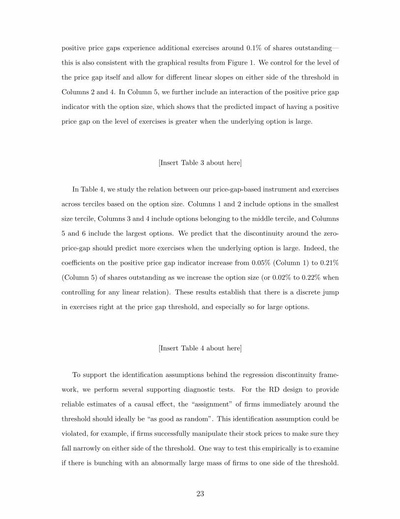
positive price gaps experience additional exercises around 0.1% of shares outstanding—

this is also consistent with the graphical results from Figure 1. We control for the level of

the price gap itself and allow for different linear slopes on either side of the threshold in

Columns 2 and 4. In Column 5, we further include an interaction of the positive price gap

indicator with the option size, which shows that the predicted impact of having a positive

price gap on the level of exercises is greater when the underlying option is large.

[Insert Table 3 about here]

In Table 4, we study the relation between our price-gap-based instrument and exercises

across terciles based on the option size. Columns 1 and 2 include options in the smallest

size tercile, Columns 3 and 4 include options belonging to the middle tercile, and Columns

5 and 6 include the largest options. We predict that the discontinuity around the zero-

price-gap should predict more exercises when the underlying option is large. Indeed, the

coefficients on the positive price gap indicator increase from 0.05% (Column 1) to 0.21%

(Column 5) of shares outstanding as we increase the option size (or 0.02% to 0.22% when

controlling for any linear relation). These results establish that there is a discrete jump

in exercises right at the price gap threshold, and especially so for large options.

[Insert Table 4 about here]

To support the identification assumptions behind the regression discontinuity frame-

work, we perform several supporting diagnostic tests. For the RD design to provide

reliable estimates of a causal effect, the “assignment” of firms immediately around the

threshold should ideally be “as good as random”. This identification assumption could be

violated, for example, if firms successfully manipulate their stock prices to make sure they

fall narrowly on either side of the threshold. One way to test this empirically is to examine

if there is bunching with an abnormally large mass of firms to one side of the threshold.

23

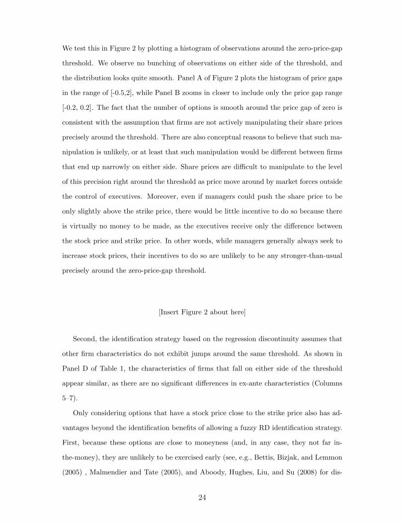
We test this in Figure 2 by plotting a histogram of observations around the zero-price-gap

threshold. We observe no bunching of observations on either side of the threshold, and

the distribution looks quite smooth. Panel A of Figure 2 plots the histogram of price gaps

in the range of [-0.5,2], while Panel B zooms in closer to include only the price gap range

[-0.2, 0.2]. The fact that the number of options is smooth around the price gap of zero is

consistent with the assumption that firms are not actively manipulating their share prices

precisely around the threshold. There are also conceptual reasons to believe that such ma-

nipulation is unlikely, or at least that such manipulation would be different between firms

that end up narrowly on either side. Share prices are difficult to manipulate to the level

of this precision right around the threshold as price move around by market forces outside

the control of executives. Moreover, even if managers could push the share price to be

only slightly above the strike price, there would be little incentive to do so because there

is virtually no money to be made, as the executives receive only the difference between

the stock price and strike price. In other words, while managers generally always seek to

increase stock prices, their incentives to do so are unlikely to be any stronger-than-usual

precisely around the zero-price-gap threshold.

[Insert Figure 2 about here]

Second, the identification strategy based on the regression discontinuity assumes that

other firm characteristics do not exhibit jumps around the same threshold. As shown in

Panel D of Table 1, the characteristics of firms that fall on either side of the threshold

appear similar, as there are no significant differences in ex-ante characteristics (Columns

5–7).

Only considering options that have a stock price close to the strike price also has ad-

vantages beyond the identification benefits of allowing a fuzzy RD identification strategy.

First, because these options are close to moneyness (and, in any case, they not far in-

the-money), they are unlikely to be exercised early (see, e.g., Bettis, Bizjak, and Lemmon

(2005) , Malmendier and Tate (2005), and Aboody, Hughes, Liu, and Su (2008) for dis-

24

cussions of incentives for early exercise). The basic reason why early exercise is unlikely in

this setting is that the time value for an option is the greatest—and early exercise the most

costly—when the stock price is close to the strike price. Early exercises could nevertheless

introduce some noise in the first stage and thereby drive down the estimated coefficients

in the first stage and reduced-form second stage. Another conceptual benefit of examining

only options with a small price gap is that we do not need to make a distinction between

firms’ incentives to manage basic versus diluted EPS: Options that only have a small price

gap are only so slightly in-the-money that the adjustment to the number of shares when

calculating diluted EPS is minimal.14

7 Main results

This section describes “second stage” results based on the fuzzy RD framework. We first

study the consequences of having a positive price gap on firms’ shares outstanding and

how changes to the denominator affect EPS. Next, we present results on repurchases.

We then examine the effect of option exercises on other strategies that firms can use

to mitigate the dilutive effects on EPS, including cutting real investment and accruals

management. Throughout, we devote special attention to settings where we may expect a

greater response to counter dilution: large options, when firms explicitly use EPS targets

in determining compensation, and for firms with positive income.

7.1 Consequences for shares outstanding and mechanical

EPS reduction

The results in the previous section showed a discontinuity in the level of exercises around

the zero-price-gap threshold. In this section, we present evidence on how these exercises

affect shares outstanding and how that, in turn, puts negative pressure on EPS.

Table 5 presents results on how firms on either side of the zero-price-gap threshold

are affected in terms of changes to shares outstanding. We estimate regressions for firm-

14See, for example, Bens et al. (2003) for details on the how to calculate diluted EPS).

25

quarters with options within a 20% window around the zero-price-gap threshold that are

of the form:

∆Sharesq−1 to q0,i = α+ β1I[Pricegapi>0] + β2Pricegapi + β3Pricegapi × I[Pricegapi>0] + εi,

In Panel A, we use the percent change in shares outstanding, which is measured as

the difference is shares between the end of the quarter of option expiration (q0) and the

previous quarter (q−1), normalized by shares outstanding in q−1. In Columns 1 and 2,

we show results for the full sample, while Columns 3–4 focus on the top size tercile of

options. Across the full sample of options, the number of shares does expand slightly but

this difference is not statistically significant, but when we focus in on only the options

in the top size tercile where the effect should be larger, the coefficients on the positive

price gap indicator become larger and more significant. For these options, the number of

shares expands by around 1.02% more for the firms that fall on the positive side of the

threshold compared to the firms on the negative side, and this effect increases to 1.58%

after controlling for any linear relation with the price gap. In Panel B, we measure the

dependent variable as changes in log shares outstanding between q0 and q−1. The results

are similar to those in Panel A and now also weakly significant even in the full sample of

option awards.

[Insert Table 5 about here]

These results on shares outstanding are notably “net” of any buybacks. That is,

the resulting expansion in shares shows that firms at least do not fully compensate for

the expansion in shares from options exercises buy repurchasing more shares. In the next

section, we will study if there is any measurable effect on buybacks at all to partly mitigate

the share expansion.

We next study the extent of the dilutive effect that this expansion in shares has on

26

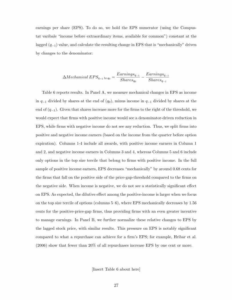
earnings per share (EPS). To do so, we hold the EPS numerator (using the Compus-

tat varibale “income before extraordinary items, available for common”) constant at the

lagged (q−1) value, and calculate the resulting change in EPS that is “mechanically” driven

by changes to the denominator:

∆Mechanical EPSq−1 to q0 =Earningsq−1

Sharesq0−Earningsq−1

Sharesq−1

Table 6 reports results. In Panel A, we measure mechanical changes in EPS as income

in q−1 divided by shares at the end of (q0), minus income in q−1 divided by shares at the

end of (q−1). Given that shares increase more for the firms to the right of the threshold, we

would expect that firms with positive income would see a denominator-driven reduction in

EPS, while firms with negative income do not see any reduction. Thus, we split firms into

positive and negative income earners (based on the income from the quarter before option

expiration). Columns 1-4 include all awards, with positive income earners in Column 1

and 2, and negative income earners in Columns 3 and 4, whereas Columns 5 and 6 include

only options in the top size tercile that belong to firms with positive income. In the full

sample of positive income earners, EPS decreases “mechanically” by around 0.68 cents for

the firms that fall on the positive side of the price-gap-threshold compared to the firms on

the negative side. When income is negative, we do not see a statistically significant effect

on EPS. As expected, the dilutive effect among the positive-income is larger when we focus

on the top size tercile of options (columns 5–6), where EPS mechanically decreases by 1.56

cents for the positive-price-gap firms, thus providing firms with an even greater incentive

to manage earnings. In Panel B, we further normalize these relative changes to EPS by

the lagged stock price, with similar results. This pressure on EPS is notably significant

compared to what a repurchase can achieve for a firm’s EPS; for example, Hribar et al.

(2006) show that fewer than 20% of all repurchases increase EPS by one cent or more.

[Insert Table 6 about here]

27

7.2 Do firms engage in anti-dilutive repurchases?

If firms do share buybacks to counter the dilutive effect of exercises, we should observe a

similar discrete jump in repurchases around the zero price gap threshold. On the other

hand, if the observed correlation between options exercises and repurchases is driven

by potentially omitted variables or reverse causality, we should not observe a jump in

repurchases at the zero-price-gap threshold.

Table 7 reports results on the effect of exercises on repurchases using the regression

discontinuity framework. Similar to the previous section, we estimate the following re-

gression for firm-quarters with options within a 20% window around the zero-price-gap

threshold:

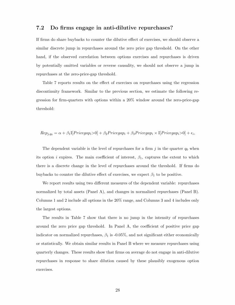
Repj,q0 = α+ β1I[Pricegapi>0] + β2Pricegapi + β3Pricegapi × I[Pricegapi>0] + εi,

The dependent variable is the level of repurchases for a firm j in the quarter q0 when

its option i expires. The main coefficient of interest, β1, captures the extent to which

there is a discrete change in the level of repurchases around the threshold. If firms do

buybacks to counter the dilutive effect of exercises, we expect β1 to be positive.

We report results using two different measures of the dependent variable: repurchases

normalized by total assets (Panel A), and changes in normalized repurchases (Panel B).

Columns 1 and 2 include all options in the 20% range, and Columns 3 and 4 includes only

the largest options.

The results in Table 7 show that there is no jump in the intensity of repurchases

around the zero price gap threshold. In Panel A, the coefficient of positive price gap

indicator on normalized repurchases, β1 is -0.05%, and not significant either economically

or statistically. We obtain similar results in Panel B where we measure repurchases using

quarterly changes. These results show that firms on average do not engage in anti-dilutive

repurchases in response to share dilution caused by these plausibly exogenous option

exercises.

28

[Insert Table 7 about here]

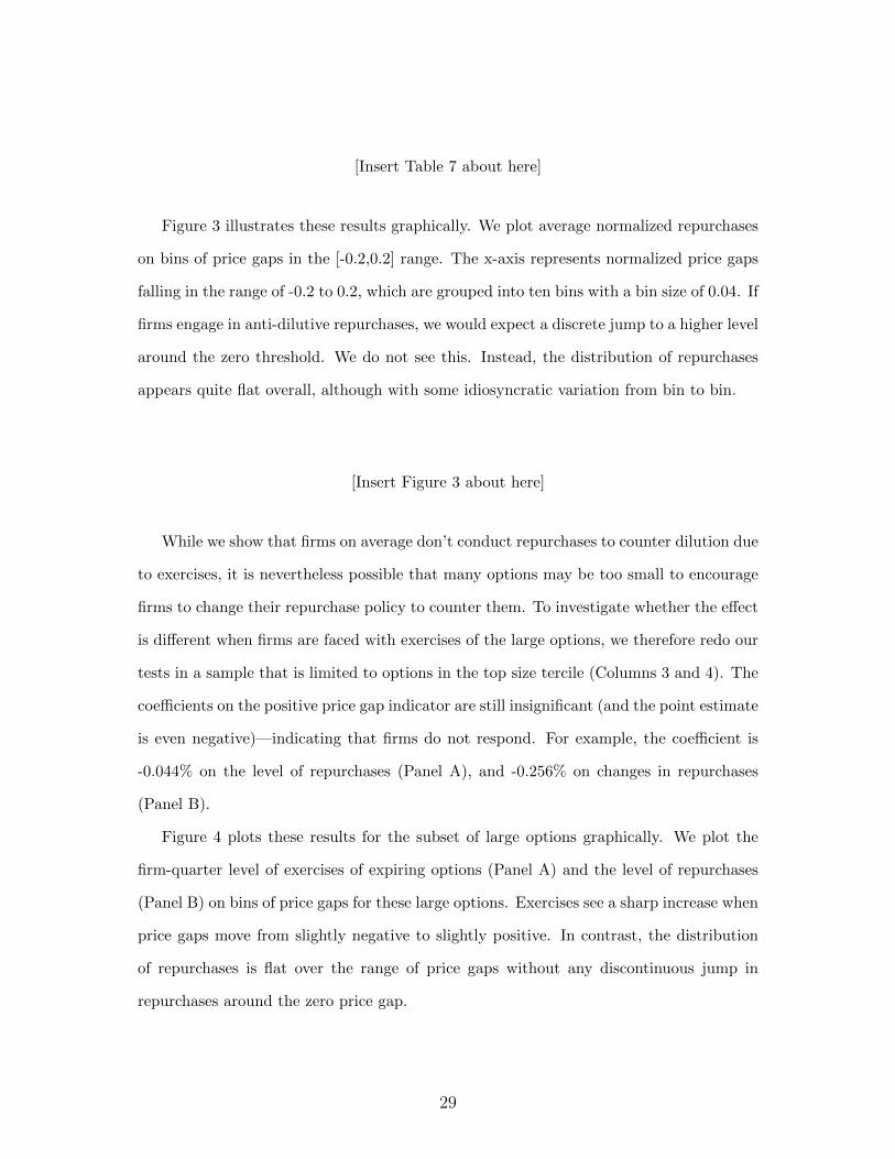
Figure 3 illustrates these results graphically. We plot average normalized repurchases

on bins of price gaps in the [-0.2,0.2] range. The x-axis represents normalized price gaps

falling in the range of -0.2 to 0.2, which are grouped into ten bins with a bin size of 0.04. If

firms engage in anti-dilutive repurchases, we would expect a discrete jump to a higher level

around the zero threshold. We do not see this. Instead, the distribution of repurchases

appears quite flat overall, although with some idiosyncratic variation from bin to bin.

[Insert Figure 3 about here]

While we show that firms on average don’t conduct repurchases to counter dilution due

to exercises, it is nevertheless possible that many options may be too small to encourage

firms to change their repurchase policy to counter them. To investigate whether the effect

is different when firms are faced with exercises of the large options, we therefore redo our

tests in a sample that is limited to options in the top size tercile (Columns 3 and 4). The

coefficients on the positive price gap indicator are still insignificant (and the point estimate

is even negative)—indicating that firms do not respond. For example, the coefficient is

-0.044% on the level of repurchases (Panel A), and -0.256% on changes in repurchases

(Panel B).

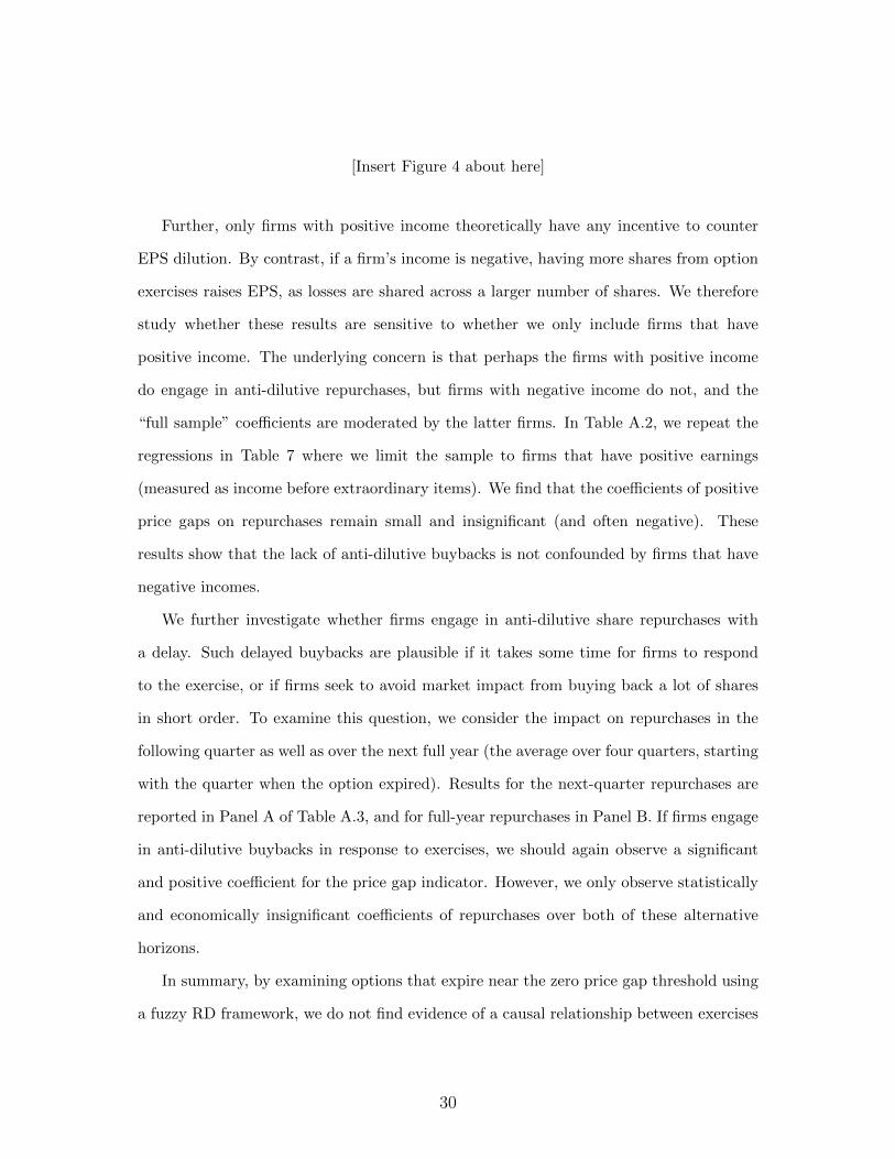
Figure 4 plots these results for the subset of large options graphically. We plot the

firm-quarter level of exercises of expiring options (Panel A) and the level of repurchases

(Panel B) on bins of price gaps for these large options. Exercises see a sharp increase when

price gaps move from slightly negative to slightly positive. In contrast, the distribution

of repurchases is flat over the range of price gaps without any discontinuous jump in

repurchases around the zero price gap.

29

[Insert Figure 4 about here]

Further, only firms with positive income theoretically have any incentive to counter

EPS dilution. By contrast, if a firm’s income is negative, having more shares from option

exercises raises EPS, as losses are shared across a larger number of shares. We therefore

study whether these results are sensitive to whether we only include firms that have

positive income. The underlying concern is that perhaps the firms with positive income

do engage in anti-dilutive repurchases, but firms with negative income do not, and the

“full sample” coefficients are moderated by the latter firms. In Table A.2, we repeat the

regressions in Table 7 where we limit the sample to firms that have positive earnings

(measured as income before extraordinary items). We find that the coefficients of positive

price gaps on repurchases remain small and insignificant (and often negative). These

results show that the lack of anti-dilutive buybacks is not confounded by firms that have

negative incomes.

We further investigate whether firms engage in anti-dilutive share repurchases with

a delay. Such delayed buybacks are plausible if it takes some time for firms to respond

to the exercise, or if firms seek to avoid market impact from buying back a lot of shares

in short order. To examine this question, we consider the impact on repurchases in the

following quarter as well as over the next full year (the average over four quarters, starting

with the quarter when the option expired). Results for the next-quarter repurchases are

reported in Panel A of Table A.3, and for full-year repurchases in Panel B. If firms engage

in anti-dilutive buybacks in response to exercises, we should again observe a significant

and positive coefficient for the price gap indicator. However, we only observe statistically

and economically insignificant coefficients of repurchases over both of these alternative

horizons.

In summary, by examining options that expire near the zero price gap threshold using

a fuzzy RD framework, we do not find evidence of a causal relationship between exercises

30

and repurchases. This holds even when we consider only the largest options and when we

consider longer time windows over which firms may conduct such repurchases.

7.3 Real and accruals-based earnings management

Option exercises exert a decreasing force on EPS due to the expansion of shares, especially

as we show that these exercises are not countered by share repurchases. Firms nevertheless

also have other tools at their disposal that can compensate for this effect by managing

the numerator, i.e. earnings. We now examine the extent to which firms instead respond

to EPS dilution from option exercises by managing earnings.

We analyze the effects on the two main tools firms have at their disposal to man-

age earnings: by cutting discretionary spending (which we proxy using changes to R&D

spending, as in (Baber et al., 1991; Dechow and Sloan, 1991; Roychowdhury, 2006)), or by

managing accruals (Dechow et al., 1995). Because firms with positive or negative income

before extraordinary items face very different incentives to engage in earnings manage-

ment when faced with option exercises (the firms with negative income experience better

EPS when faced with dilution), we further partition the sample by the sign of income.

Table 8 presents results of the effects of price gaps on real (Panel A) and accruals-based

(Panel B) earnings management.

[Insert Table 8 about here]

In Panel A, we show that firms with positive price gaps decrease R&D investment more

than the ones with negative price gaps. This effect is significant only among firms that

have positive income. The firms with negative income here thus also serve as a kind of

placebo: If there were some still-omitted spurious factor that was causing a discontinuous

effect around the threshold, we would expect that factor to also be at work for the firms

with negative income.

In Panel B, we examine whether the firms that end up on either side of the zero-price-

gap threshold differentially alter their accruals. We employ three measures of accruals:

31

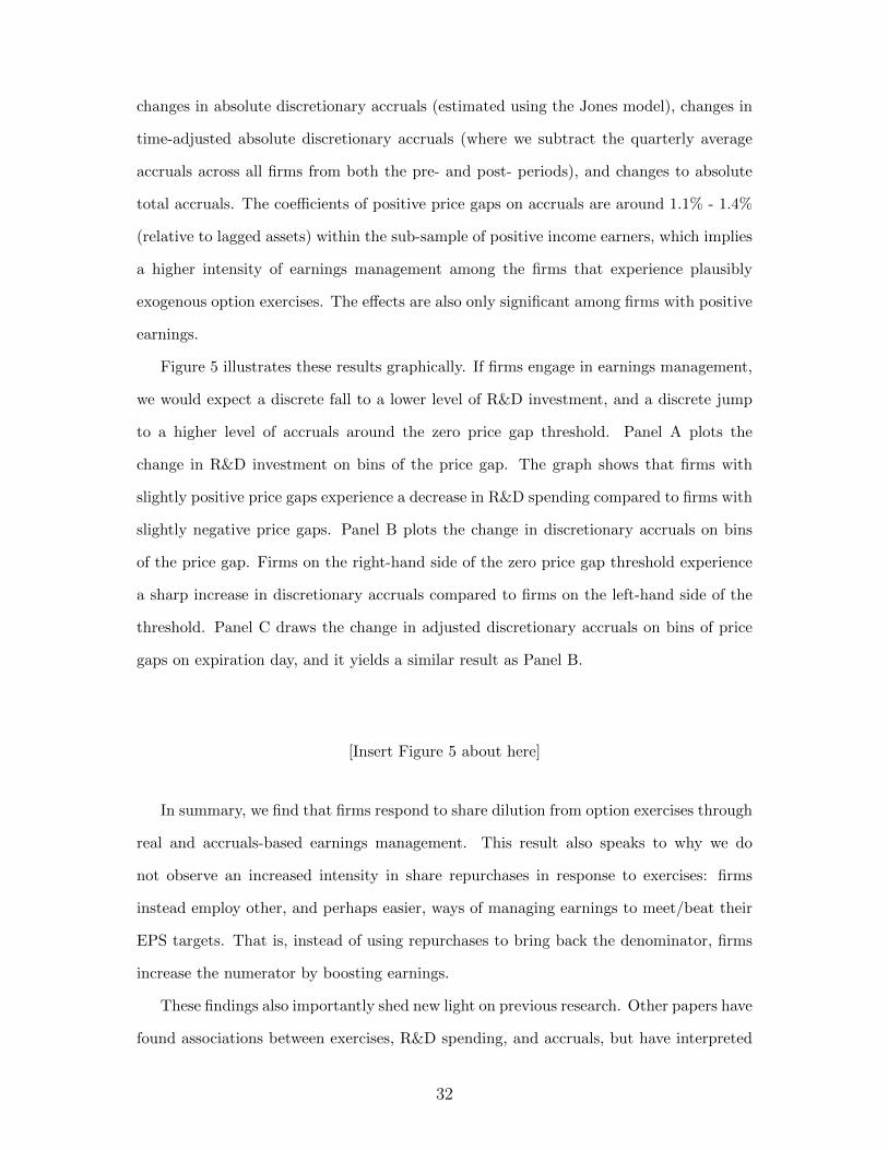
changes in absolute discretionary accruals (estimated using the Jones model), changes in

time-adjusted absolute discretionary accruals (where we subtract the quarterly average

accruals across all firms from both the pre- and post- periods), and changes to absolute

total accruals. The coefficients of positive price gaps on accruals are around 1.1% - 1.4%

(relative to lagged assets) within the sub-sample of positive income earners, which implies

a higher intensity of earnings management among the firms that experience plausibly

exogenous option exercises. The effects are also only significant among firms with positive

earnings.

Figure 5 illustrates these results graphically. If firms engage in earnings management,

we would expect a discrete fall to a lower level of R&D investment, and a discrete jump

to a higher level of accruals around the zero price gap threshold. Panel A plots the

change in R&D investment on bins of the price gap. The graph shows that firms with

slightly positive price gaps experience a decrease in R&D spending compared to firms with

slightly negative price gaps. Panel B plots the change in discretionary accruals on bins

of the price gap. Firms on the right-hand side of the zero price gap threshold experience

a sharp increase in discretionary accruals compared to firms on the left-hand side of the

threshold. Panel C draws the change in adjusted discretionary accruals on bins of price

gaps on expiration day, and it yields a similar result as Panel B.

[Insert Figure 5 about here]

In summary, we find that firms respond to share dilution from option exercises through

real and accruals-based earnings management. This result also speaks to why we do

not observe an increased intensity in share repurchases in response to exercises: firms

instead employ other, and perhaps easier, ways of managing earnings to meet/beat their

EPS targets. That is, instead of using repurchases to bring back the denominator, firms

increase the numerator by boosting earnings.

These findings also importantly shed new light on previous research. Other papers have

found associations between exercises, R&D spending, and accruals, but have interpreted

32

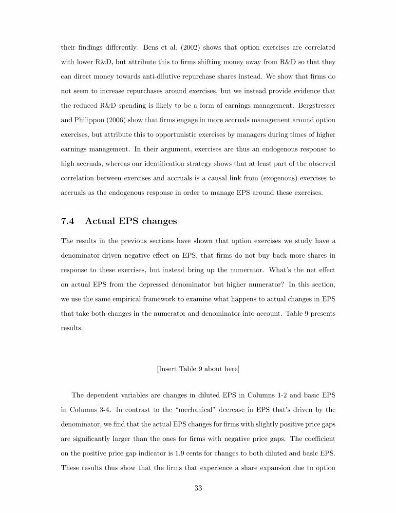
their findings differently. Bens et al. (2002) shows that option exercises are correlated

with lower R&D, but attribute this to firms shifting money away from R&D so that they

can direct money towards anti-dilutive repurchase shares instead. We show that firms do

not seem to increase repurchases around exercises, but we instead provide evidence that

the reduced R&D spending is likely to be a form of earnings management. Bergstresser

and Philippon (2006) show that firms engage in more accruals management around option

exercises, but attribute this to opportunistic exercises by managers during times of higher

earnings management. In their argument, exercises are thus an endogenous response to

high accruals, whereas our identification strategy shows that at least part of the observed

correlation between exercises and accruals is a causal link from (exogenous) exercises to

accruals as the endogenous response in order to manage EPS around these exercises.

7.4 Actual EPS changes

The results in the previous sections have shown that option exercises we study have a

denominator-driven negative effect on EPS, that firms do not buy back more shares in

response to these exercises, but instead bring up the numerator. What’s the net effect

on actual EPS from the depressed denominator but higher numerator? In this section,

we use the same empirical framework to examine what happens to actual changes in EPS

that take both changes in the numerator and denominator into account. Table 9 presents

results.

[Insert Table 9 about here]

The dependent variables are changes in diluted EPS in Columns 1-2 and basic EPS

in Columns 3-4. In contrast to the “mechanical” decrease in EPS that’s driven by the

denominator, we find that the actual EPS changes for firms with slightly positive price gaps

are significantly larger than the ones for firms with negative price gaps. The coefficient

on the positive price gap indicator is 1.9 cents for changes to both diluted and basic EPS.

These results thus show that the firms that experience a share expansion due to option

33

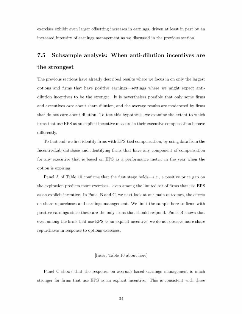
exercises exhibit even larger offsetting increases in earnings, driven at least in part by an

increased intensity of earnings management as we discussed in the previous section.

7.5 Subsample analysis: When anti-dilution incentives are

the strongest

The previous sections have already described results where we focus in on only the largest

options and firms that have positive earnings—settings where we might expect anti-

dilution incentives to be the stronger. It is nevertheless possible that only some firms

and executives care about share dilution, and the average results are moderated by firms

that do not care about dilution. To test this hypothesis, we examine the extent to which

firms that use EPS as an explicit incentive measure in their executive compensation behave

differently.

To that end, we first identify firms with EPS-tied compensation, by using data from the

IncentiveLab database and identifying firms that have any component of compensation

for any executive that is based on EPS as a performance metric in the year when the

option is expiring.

Panel A of Table 10 confirms that the first stage holds—i.e., a positive price gap on

the expiration predicts more exercises—even among the limited set of firms that use EPS

as an explicit incentive. In Panel B and C, we next look at our main outcomes, the effects

on share repurchases and earnings management. We limit the sample here to firms with

positive earnings since these are the only firms that should respond. Panel B shows that

even among the firms that use EPS as an explicit incentive, we do not observe more share

repurchases in response to options exercises.

[Insert Table 10 about here]

Panel C shows that the response on accruals-based earnings management is much

stronger for firms that use EPS as an explicit incentive. This is consistent with these

34

firms being more concerned about the dilution from option exercises. By contrast, we see

no response among the firms that do not use EPS as an incentive. This is consistent with

managers being more concerned about maintaining the EPS around dilution only when

they are compensated for doing so. The sample of firms with no EPS incentive also serves

as yet another “placebo” test, as we would expect a smaller response among these firms.15

8 Robustness tests

This section discusses further tests that we employ to assess the robustness of our results.

In our baseline results, we do not include observations with missing data for the “pur-

chase of common and preferred stocks” variable in Compustat. We, therefore, redo our

tests where we set any missing data to zero. The results remain similar. We also examine

whether our results are sensitive to different ways of measuring repurchases. We adjust

our repurchase measure for lagged repurchases, by subtracting the average repurchases

during the last four quarters from the current quarter, again with similar results. We also

adjust the repurchases by average repurchase in the same industry and quarter (industry

classifications based on the Fama-French 49 industries). Another repurchase measurement

uses a repurchase indicator, which takes on a value of one if there is a repurchase in the

quarter; and zero, otherwise.

We also collect data from the SDC database on repurchase announcements to examine

whether such announcements are more likely in quarters when options are exercised using

the same regression discontinuity framework as above, but we find no evidence of an

increased likelihood of new repurchase programs. These results on announcements are

thus consistent with our baseline results that focus on actual repurchases.

We further test whether our results are sensitive to variations to our regression dis-

continuity specification. We examine whether our results are sensitive to the window size

around the threshold of a zero price gap, by changing the window to [-0.15, 0.15], [-0.25,

15We nevertheless do not see a significant differential effect on R&D in this limited sample. Part of the reasonis that the sample of firms that report R&D is significantly smaller, so when we further limit this sample tofirms that we can link to IncentiveLab that use EPS and have positive income, we end up with a very smallsample and thus insufficient statistical power to tell any differences apart.

35

0.25], [-0.3, 0.3], [-0.35, 0.35], and [-0.4, 0.4]. We also include the square of the price

gap in the regression to account for a non-linear effect of the assignment variable. Table

11 reports the regression coefficients of the positive price gap indicator across a range of

different bandwidths. The dependent variables include option exercises and repurchases

in Panel A, and earnings management variables in Panel B. The bandwidths range from

0.15 to 0.4 with an interval of 0.05. We also include the “optimal” bandwidth based on

Calonico, Cattaneo, Titiunik et al. (2014), which is 0.33. For bandwidths smaller than

or equal to 0.2, we control for the linear relation with price gap, and for bandwidths

larger than 0.2, we control for the linear and quadratic relation with price gap. In Panel

A, the coefficients of the positive price gap indicator are significantly positive on option

exercises and not significant on repurchases across all alternative bandwidths. In Panel

B, the coefficients of the positive price gap are significantly negative on the change in

investment for a majority of the bandwidths, and are significantly positive on the change

in discretionary accruals in all alternative windows. These findings show that the previous

results are robust to alternative estimation windows.

[Insert Table 11 about here]

We also check the effect of the price gap on pre-trends of outcome variables. We

examine pre-trends in shares outstanding and earnings management in quarters before

option expiration in Table A.4 in the Appendix. The pre-trend outcome variables are

measured as the average change in the previous four quarters. We find that there are no

such pre-trends in the quarters before the option expiration.

9 Concluding remarks

Many previous studies have shown a positive correlation between option exercises and

share repurchases and argue that firms may seek to engage in shares buybacks to counter

EPS dilution from options compensation. This correlation may nevertheless not necessar-

36

ily be causal. Both exercises and share repurchases are endogenous decisions that depend

on several third factors such as firm performance and life cycle and which may not all

be easy to control for, and firms have at their disposal alternative tools they can use to

manage EPS.

This paper examines this question using a regression discontinuity framework to iden-

tify the causal impact of quasi-exogenous option exercises on the two main ways of man-

aging EPS: share repurchases and earnings management. We exploit a fuzzy regression

discontinuity framework that focuses on options with stock prices that are close to money-

ness and examine responses by firms that experience quasi-exogenous exercises because of

their options ending up slightly in-the-money. Contrary to an “anti-dilution hypothesis”,

our results show that these quasi-exogenous exercises do not cause additional buybacks.

In other words, even though firms with many options and options that are in-the-money

tend to do more buybacks on average, this difference disappears once we zoom in on a

smaller window where other confounding factors are held constant and where we should

observe a discrete jump if firms engage in anti-dilutive repurchases. Instead, we show that

firms engage in real- and accrual-based earnings management to avoid depressing EPS

around option exercises.

Our results are thus most consistent with the survey evidence of Graham et al. (2005),

who report that real- and accruals-based earnings management tend to be much preferred

to buybacks among executives looking to meet EPS targets, and cohen2008real who show

that outstanding options are positively correlated with accruals-based earnings manage-

ment.

If firms do not engage in share repurchases to manage earnings around option exercises,

why do so many managers give answers to survey questions suggestion that anti-dilution

is one of the main reasons for buying back shares? We can of course only speculate why

managers answer the way they do. One possibility is that managers who have repurchased

shares clearly notice that one of the “uses” for the resulting treasury stock is to provide

shares in connection with option exercises; but the real reason for having originally repur-

chased shares could still have been something else, such as flexibility or tax efficiency. In

other words, using the treasury stock for option exercises does not mean that the reason

37

for doing those repurchases was because the firm anticipated those exercises, or that a

firm would have done more or less buybacks if it faced a different magnitude of option

exercises.

Finally, we want to emphasize that it is still possible that other aspects of options

compensation could have a causal effect on payout policy, including the fact that options

typically are not dividend-protected. While our empirical framework is well-suited to

directly testing the causal effect of a dilution channel, we cannot take a stand on these

other possible mechanisms that link options with payout policy, and which are worthy of

further study.

38

References

Aboody, D., J. Hughes, J. Liu, and W. Su. 2008. Are executive stock option exercises

driven by private information? Review of Accounting Studies 13:551–570.

Almeida, H., V. Fos, and M. Kronlund. 2016. The real effects of share repurchases. Journal

of Financial Economics 119:168–185.

Almond, D., and J. J. Doyle. 2011. After midnight: A regression discontinuity design in

length of postpartum hospital stays. American Economic Journal: Economic Policy

3:1–34.

Angrist, J. D., and V. Lavy. 1999. Using Maimonides’ rule to estimate the effect of class

size on scholastic achievement. The Quarterly Journal of Economics 114:533–575.

Babenko, I. 2009. Share repurchases and pay-performance sensitivity of employee com-

pensation contracts. The Journal of Finance 64:117–150.

Babenko, I., M. Lemmon, and Y. Tserlukevich. 2011. Employee stock options and invest-

ment. The Journal of Finance 66:981–1009.

Baber, W. R., P. M. Fairfield, and J. A. Haggard. 1991. The effect of concern about

reported income on discretionary spending decisions: The case of research and devel-

opment. Accounting Review pp. 818–829.

Bagwell, L. S. 1991. Share repurchase and takeover deterrence. The RAND Journal of

Economics pp. 72–88.

Bagwell, L. S., and J. B. Shoven. 1989. Cash distributions to shareholders. The Journal

of Economic Perspectives 3:129–140.

Baker, T., D. Collins, and A. Reitenga. 2003. Stock option compensation and earnings

management incentives. Journal of Accounting, Auditing & Finance 18:557–582.

Banyi, M., E. A. Dyl, and K. M. Kahle. 2005. Measuring share repurchases. Working

paper.

39

Bens, D. A., V. Nagar, D. J. Skinner, and M. F. Wong. 2003. Employee stock options,

EPS dilution, and stock repurchases. Journal of Accounting and Economics 36:51–90.

Bens, D. A., V. Nagar, and M. Wong. 2002. Real investment implications of employee

stock option exercises. Journal of Accounting Research 40:359–393.

Bergstresser, D., and T. Philippon. 2006. CEO incentives and earnings management.

Journal of Financial Economics 80:511–529.

Bettis, J. C., J. M. Bizjak, and M. L. Lemmon. 2005. Exercise behavior, valuation, and the

incentive effects of employee stock options. Journal of Financial Economics 76:445–470.

Billett, M. T., and H. Xue. 2007. The takeover deterrent effect of open market share

repurchases. The Journal of Finance 62:1827–1850.

Brav, A., J. R. Graham, C. R. Harvey, and R. Michaely. 2005. Payout policy in the 21st

century. Journal of Financial Economics 77:483–527.

Bushee, B. J. 1998. The influence of institutional investors on myopic R&D investment

behavior. Accounting review pp. 305–333.

Cahuc, P., S. Carcillo, and T. Le Barbanchon. 2014. Do hiring credits work in recessions?

Evidence from France .

Calonico, S., M. D. Cattaneo, R. Titiunik, et al. 2014. Robust data-driven inference in

the regression-discontinuity design. Stata Journal 14:909–946.

Carpenter, J. N., and B. Remmers. 2001. Executive stock option exercises and inside

information. The Journal of Business 74:513–534.

Carpenter, J. N., R. Stanton, and N. Wallace. 2010. Optimal exercise of executive stock

options and implications for firm cost. Journal of Financial Economics 98:315–337.

Chauvin, K. W., and C. Shenoy. 2001. Stock price decreases prior to executive stock

option grants. Journal of Corporate Finance 7:53–76.

40

Chava, S., and A. Purnanandam. 2010. CEOs versus CFOs: Incentives and corporate

policies. Journal of Financial Economics 97:263–278.

Cheng, Y., J. Harford, and T. T. Zhang. 2015. Bonus-driven repurchases. Journal of

Financial and Quantitative Analysis 50:447–475.

Coggan, P. 2015. The share buyback mirage. URL https://www.economist.com/

buttonwoods-notebook/2015/10/06/the-share-buyback-mirage.

Cohen, D. A., A. Dey, and T. Z. Lys. 2008. Real and accrual-based earnings management

in the pre-and post-Sarbanes-Oxley periods. The Accounting Review 83:757–787.

Cook, D. O., L. Krigman, and J. C. Leach. 2003. On the timing and execution of open

market repurchases. Review of Financial Studies 17:463–498.

Cornett, M. M., A. J. Marcus, and H. Tehranian. 2008. Corporate governance and pay-

for-performance: The impact of earnings management. Journal of Financial Economics

87:357–373.

Dechow, P. M., and R. G. Sloan. 1991. Executive incentives and the horizon problem: An

empirical investigation. Journal of Accounting and Economics 14:51–89.

Dechow, P. M., R. G. Sloan, and A. P. Sweeney. 1995. Detecting earnings management.

Accounting review pp. 193–225.

Desai, M. A., and L. Jin. 2011. Institutional tax clienteles and payout policy. Journal of

Financial Economics 100:68–84.

Erickson, T., and T. M. Whited. 2000. Measurement error and the relationship between

investment and q. Journal of Political Economy 108:1027–1057.

Fama, E. F., and K. R. French. 2001. Disappearing dividends: changing firm character-

istics or lower propensity to pay? Journal of Financial economics 60:3–43.

Fenn, G. W., and N. Liang. 2001. Corporate payout policy and managerial stock incen-

tives. Journal of Financial Economics 60:45–72.

41

Ferri, F., and N. Li. 2016. The Effect of Option-based Compensation on Payout Policy:

Evidence from FAS123R. Working paper.

Fos, V., and W. Jiang. 2015. Out-of-the-money CEOs: Private control premium and

option exercises. Review of Financial Studies 29:1549–1585.

Graham, J. R., C. R. Harvey, and S. Rajgopal. 2005. The economic implications of

corporate financial reporting. Journal of Accounting and Economics 40:3–73.

Heath, C., S. Huddart, and M. Lang. 1999. Psychological factors and stock option exercise.

The Quarterly Journal of Economics 114:601–627.

Hillert, A., E. Maug, and S. Obernberger. 2016. Stock repurchases and liquidity. Journal

of Financial Economics 119:186–209.

Hribar, P., N. T. Jenkins, and W. B. Johnson. 2006. Stock repurchases as an earnings

management device. Journal of Accounting and Economics 41:3–27.

Ikenberry, D., J. Lakonishok, and T. Vermaelen. 1995. Market underreaction to open

market share repurchases. Journal of Financial Economics 39:181–208.

Jensen, M. C. 1986. Agency costs of free cash flow, corporate finance, and takeovers. The

American Economic Review 76:323–329.

Jensen, M. V., and L. H. Pedersen. 2016. Early option exercise: Never say never. Journal

of Financial Economics 121:278–299.

Kahle, K. M. 2002. When a buyback isn’t a buyback: Open market repurchases and

employee options. Journal of Financial Economics 63:235–261.

Klein, D., and E. G. Maug. 2011. How do executives exercise their stock options? .

Lambert, R. A., W. N. Lanen, and D. F. Larcker. 1989. Executive stock option plans and

corporate dividend policy. Journal of Financial and Quantitative Analysis 24:409–425.

Larcker, D. F. 2003. Discussion of eployee stock options, EPS dilution, and stock repur-

chases. Journal of Accounting and Economics 36:45–49.

42

Liljeblom, E., and D. Pasternack. 2006. Share repurchases, dividends and executive op-

tions: The effect of dividend protection. European Financial Management 12:7–28.

Malmendier, U., and G. Tate. 2005. CEO overconfidence and corporate investment. The

Journal of Finance 60:2661–2700.

Merton, R. C. 1973. Theory of rational option pricing. The Bell Journal of economics

and management science pp. 141–183.

Rau, T., M. Sarzosa, and S. Urzua. 2015. The Children of the Missed Pill: Unintended

Consequences of Price Collusion .

Roychowdhury, S. 2006. Earnings management through real activities manipulation. Jour-

nal of Accounting and Economics 42:335–370.

Skinner, D. J., and R. G. Sloan. 2002. Earnings surprises, growth expectations, and stock

returns or don’t let an earnings torpedo sink your portfolio. Review of Accounting

Studies 7:289–312.

Van der Klaauw, W. 2002. Estimating the effect of financial aid offers on college enroll-

ment: A regression–discontinuity approach. International Economic Review 43:1249–

1287.

Weisbenner, S. 2000. Corporate share repurchases in the 1990s: What role do stock

options play?

Yermack, D. 1997. Good timing: CEO stock option awards and company news announce-

ments. The Journal of Finance 52:449–476.

43

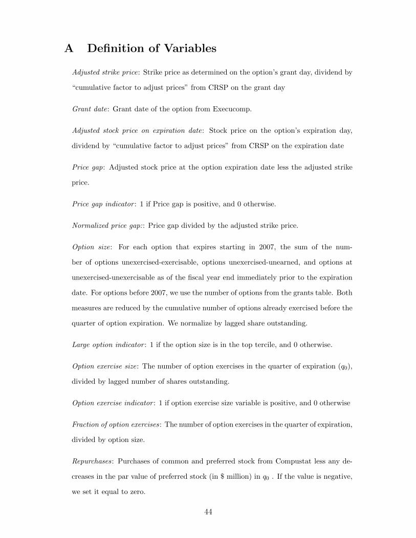
A Definition of Variables

Adjusted strike price: Strike price as determined on the option’s grant day, dividend by

“cumulative factor to adjust prices” from CRSP on the grant day

Grant date: Grant date of the option from Execucomp.

Adjusted stock price on expiration date: Stock price on the option’s expiration day,

dividend by “cumulative factor to adjust prices” from CRSP on the expiration date

Price gap: Adjusted stock price at the option expiration date less the adjusted strike

price.

Price gap indicator : 1 if Price gap is positive, and 0 otherwise.

Normalized price gap:: Price gap divided by the adjusted strike price.

Option size: For each option that expires starting in 2007, the sum of the num-

ber of options unexercised-exercisable, options unexercised-unearned, and options at

unexercised-unexercisable as of the fiscal year end immediately prior to the expiration

date. For options before 2007, we use the number of options from the grants table. Both

measures are reduced by the cumulative number of options already exercised before the

quarter of option expiration. We normalize by lagged share outstanding.

Large option indicator : 1 if the option size is in the top tercile, and 0 otherwise.

Option exercise size: The number of option exercises in the quarter of expiration (q0),

divided by lagged number of shares outstanding.

Option exercise indicator : 1 if option exercise size variable is positive, and 0 otherwise

Fraction of option exercises: The number of option exercises in the quarter of expiration,

divided by option size.

Repurchases: Purchases of common and preferred stock from Compustat less any de-

creases in the par value of preferred stock (in $ million) in q0 . If the value is negative,

we set it equal to zero.

44

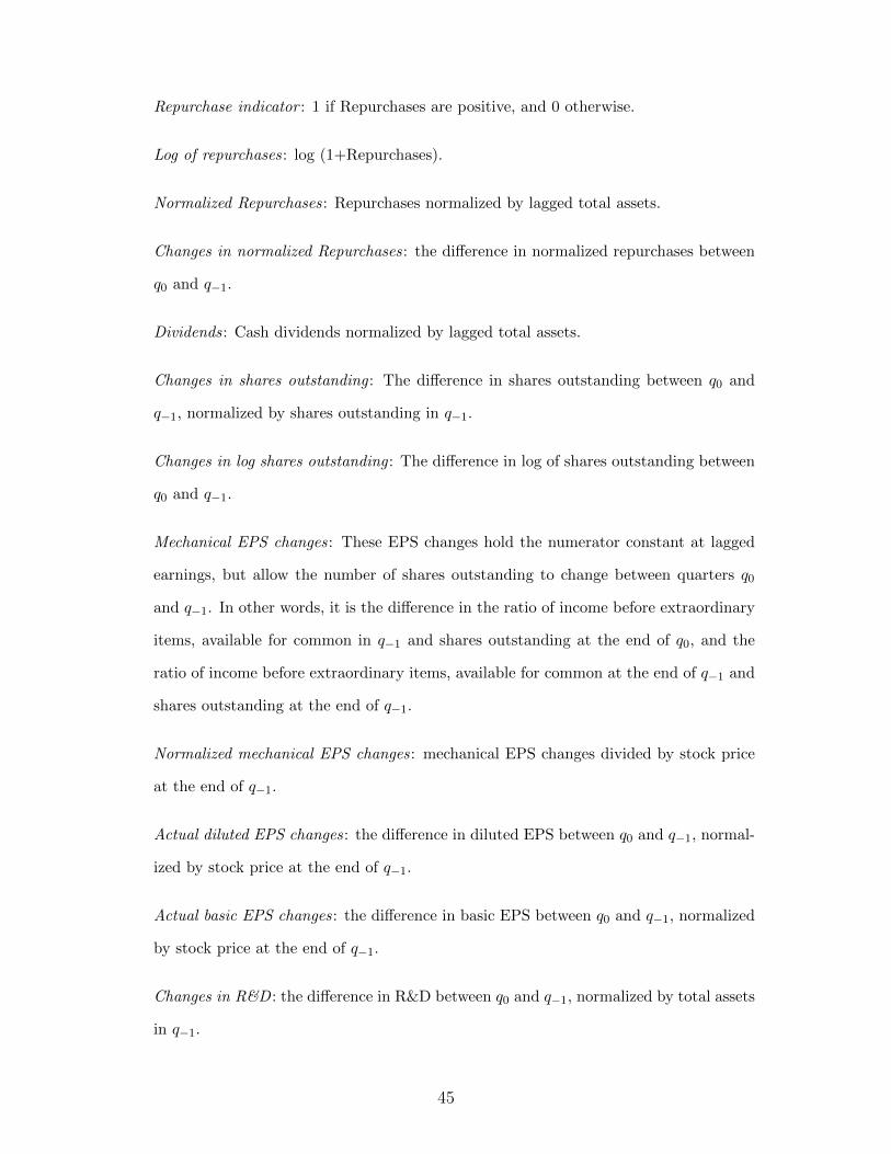
Repurchase indicator : 1 if Repurchases are positive, and 0 otherwise.

Log of repurchases: log (1+Repurchases).

Normalized Repurchases: Repurchases normalized by lagged total assets.

Changes in normalized Repurchases: the difference in normalized repurchases between

q0 and q−1.

Dividends: Cash dividends normalized by lagged total assets.

Changes in shares outstanding : The difference in shares outstanding between q0 and

q−1, normalized by shares outstanding in q−1.

Changes in log shares outstanding : The difference in log of shares outstanding between

q0 and q−1.

Mechanical EPS changes: These EPS changes hold the numerator constant at lagged

earnings, but allow the number of shares outstanding to change between quarters q0

and q−1. In other words, it is the difference in the ratio of income before extraordinary

items, available for common in q−1 and shares outstanding at the end of q0, and the

ratio of income before extraordinary items, available for common at the end of q−1 and

shares outstanding at the end of q−1.

Normalized mechanical EPS changes: mechanical EPS changes divided by stock price

at the end of q−1.

Actual diluted EPS changes: the difference in diluted EPS between q0 and q−1, normal-

ized by stock price at the end of q−1.

Actual basic EPS changes: the difference in basic EPS between q0 and q−1, normalized

by stock price at the end of q−1.

Changes in R&D : the difference in R&D between q0 and q−1, normalized by total assets

in q−1.

45

Changes in discretionary accruals: the differences in absolute residuals from the Jones’

model between q0 and q−1

Changes in adjusted discretionary accruals: the differences in absolute residuals from

the Jones model adjusted by quarters between q0 and q−1

Changes in total accruals: the differences in net income, minus changes in assets, plus

changes in liabilities, and plus depreciation in absolute value between q0 and q−1

Book-to-market : the number of shares outstanding multiplies by stock price at the end

of q−1, divided by shareholders’ equity minus preferred stock value.

Cash flow to assets: net income plus depreciation in q−1, normalized by lagged total

assets

Cash to assets: cash and short-term investment in q−1, normalized by lagged total

assets

Return on assets: net income in q−1 multiplies by four, normalized by lagged total

assets

Total debt to assets: the sum of log-term debt and current liabilities in q−1, normalized

by total assets

Log of assets: log of one plus total assets in q−1

EPS indicator : 1 if the firm’s annual proxy statement mentions “EPS” or “Earnings

per share”, or if at least one incentive granted or expiring in that fiscal year includes

EPS as a measure; and 0 otherwise.

46

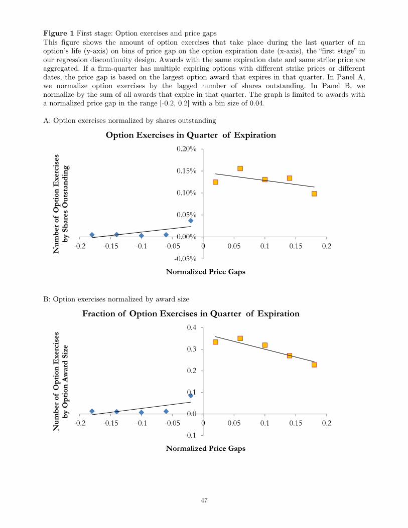
47

Figure 1 First stage: Option exercises and price gaps This figure shows the amount of option exercises that take place during the last quarter of an option’s life (y-axis) on bins of price gap on the option expiration date (x-axis), the “first stage” in our regression discontinuity design. Awards with the same expiration date and same strike price are aggregated. If a firm-quarter has multiple expiring options with different strike prices or different dates, the price gap is based on the largest option award that expires in that quarter. In Panel A, we normalize option exercises by the lagged number of shares outstanding. In Panel B, we normalize by the sum of all awards that expire in that quarter. The graph is limited to awards with a normalized price gap in the range [-0.2, 0.2] with a bin size of 0.04. A: Option exercises normalized by shares outstanding

B: Option exercises normalized by award size

-0.05%

0.00%

0.05%

0.10%

0.15%

0.20%

-0.2 -0.15 -0.1 -0.05 0 0.05 0.1 0.15 0.2

Nu

mb

er o

f O

pti

on E

xerc

ises

b

y Sh

ares

Ou

tsta

nd

ing

Normalized Price Gaps

Option Exercises in Quarter of Expiration

-0.1

0.0

0.1

0.2

0.3

0.4

-0.2 -0.15 -0.1 -0.05 0 0.05 0.1 0.15 0.2

Nu

mb

er o

f O

pti

on E

xerc

ises

b

y O

pti

on A

war

d S

ize

Normalized Price Gaps

Fraction of Option Exercises in Quarter of Expiration

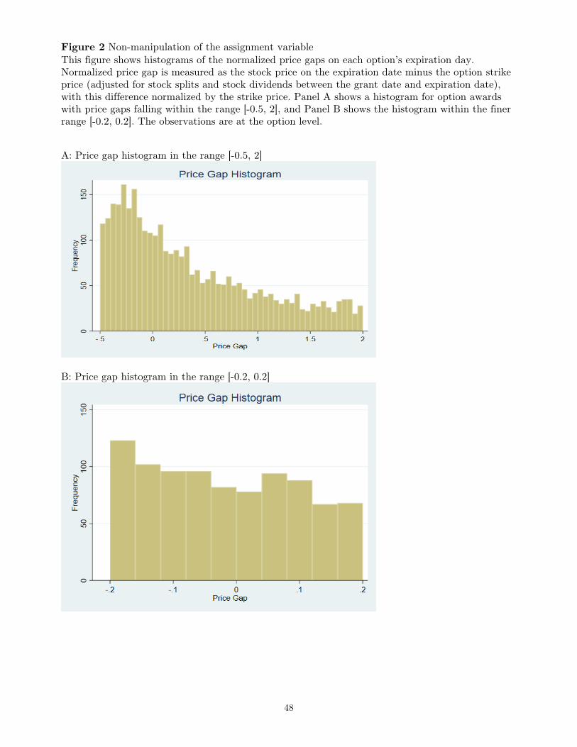
48

Figure 2 Non-manipulation of the assignment variable This figure shows histograms of the normalized price gaps on each option’s expiration day. Normalized price gap is measured as the stock price on the expiration date minus the option strike price (adjusted for stock splits and stock dividends between the grant date and expiration date), with this difference normalized by the strike price. Panel A shows a histogram for option awards with price gaps falling within the range [-0.5, 2], and Panel B shows the histogram within the finer range [-0.2, 0.2]. The observations are at the option level.

A: Price gap histogram in the range [-0.5, 2]

B: Price gap histogram in the range [-0.2, 0.2]

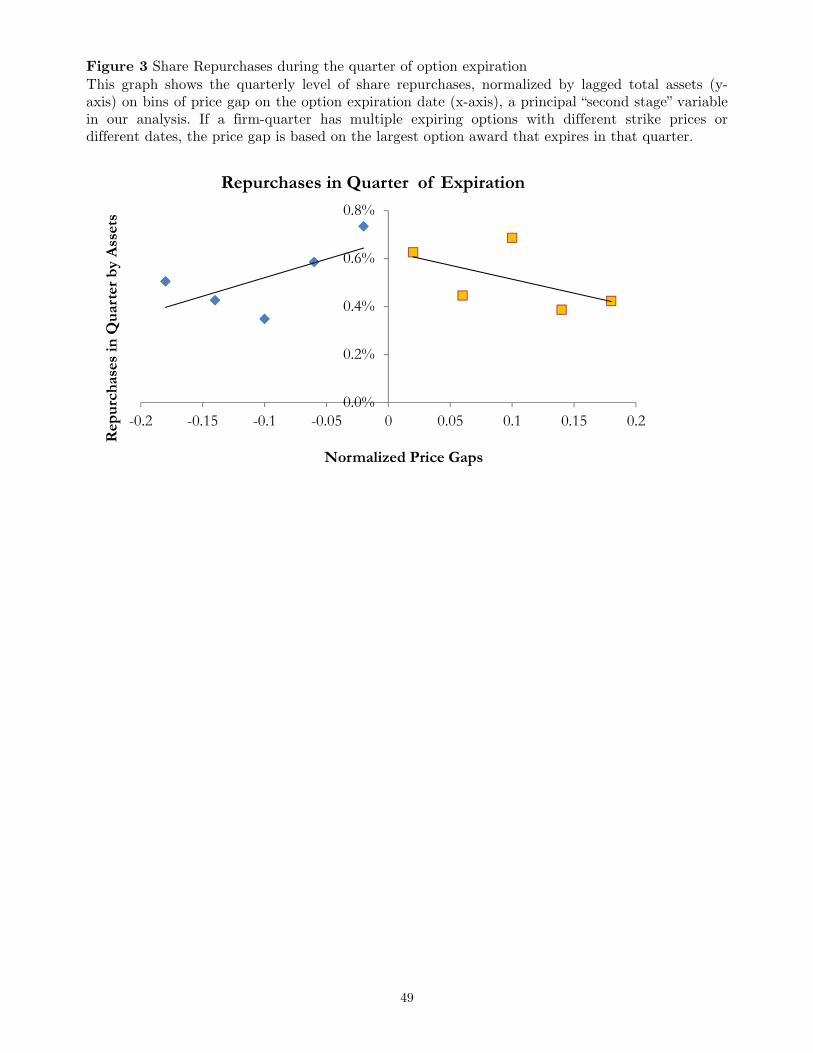
49

Figure 3 Share Repurchases during the quarter of option expiration This graph shows the quarterly level of share repurchases, normalized by lagged total assets (y-axis) on bins of price gap on the option expiration date (x-axis), a principal “second stage” variable in our analysis. If a firm-quarter has multiple expiring options with different strike prices or different dates, the price gap is based on the largest option award that expires in that quarter.

0.0%

0.2%

0.4%

0.6%

0.8%

-0.2 -0.15 -0.1 -0.05 0 0.05 0.1 0.15 0.2

Rep

urc

has

es in

Qu

arte

r b

y A

sset

s

Normalized Price Gaps

Repurchases in Quarter of Expiration

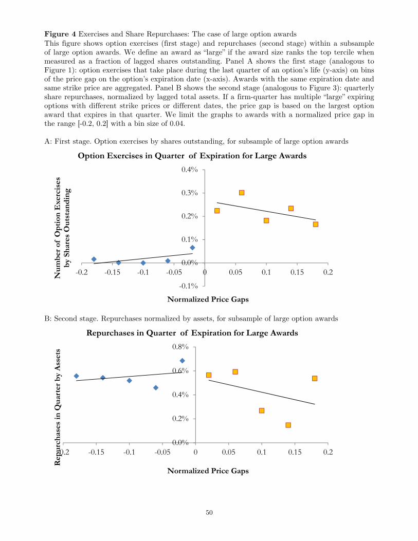
50

Figure 4 Exercises and Share Repurchases: The case of large option awards This figure shows option exercises (first stage) and repurchases (second stage) within a subsample of large option awards. We define an award as “large” if the award size ranks the top tercile when measured as a fraction of lagged shares outstanding. Panel A shows the first stage (analogous to Figure 1): option exercises that take place during the last quarter of an option’s life (y-axis) on bins of the price gap on the option’s expiration date (x-axis). Awards with the same expiration date and same strike price are aggregated. Panel B shows the second stage (analogous to Figure 3): quarterly share repurchases, normalized by lagged total assets. If a firm-quarter has multiple “large” expiring options with different strike prices or different dates, the price gap is based on the largest option award that expires in that quarter. We limit the graphs to awards with a normalized price gap in the range [-0.2, 0.2] with a bin size of 0.04. A: First stage. Option exercises by shares outstanding, for subsample of large option awards

B: Second stage. Repurchases normalized by assets, for subsample of large option awards

-0.1%

0.0%

0.1%

0.2%

0.3%

0.4%

-0.2 -0.15 -0.1 -0.05 0 0.05 0.1 0.15 0.2Nu

mb

er o

f O

pti

on E

xerc

ises

b

y Sh

ares

Ou

tsta

nd

ing

Normalized Price Gaps

Option Exercises in Quarter of Expiration for Large Awards

0.0%

0.2%

0.4%

0.6%

0.8%

-0.2 -0.15 -0.1 -0.05 0 0.05 0.1 0.15 0.2

Rep

urc

has

es in

Qu

arte

r b

y A

sset

s

Normalized Price Gaps

Repurchases in Quarter of Expiration for Large Awards

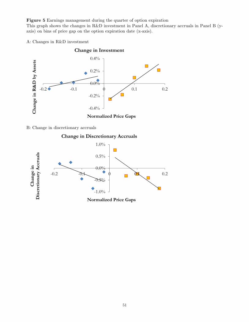
51

Figure 5 Earnings management during the quarter of option expiration This graph shows the changes in R&D investment in Panel A, discretionary accruals in Panel B (y-axis) on bins of price gap on the option expiration date (x-axis). A: Changes in R&D investment

B: Change in discretionary accruals

-0.4%

-0.2%

0.0%

0.2%

0.4%

-0.2 -0.1 0 0.1 0.2

Ch

ange

in R

&D

by

Ass

ets

Normalized Price Gaps

Change in Investment

-1.0%

-0.5%

0.0%

0.5%

1.0%

-0.2 -0.1 0 0.1 0.2

Ch

ange

in

Dis

cret

ion

ary

Acc

rual

s

Normalized Price Gaps

Change in Discretionary Accruals

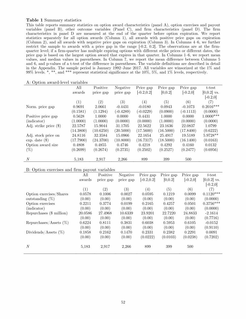
52

Table 1 Summary statistics This table reports summary statistics on option award characteristics (panel A), option exercises and payout variables (panel B), other outcome variables (Panel C), and firm characteristics (panel D). The firm characteristics in panel D are measured at the end of the quarter before option expiration. We report statistics separately for all option awards (Column 1), all awards with positive price gaps on expiration (Column 2), and all awards with negative price gaps on expiration (Column 3). In Columns 4–6, we further restrict the sample to awards with a price gap in the range [-0.2, 0.2]. The observations are at the firm-quarter level; if a firm-quarter has multiple expiring options with different strike prices or different dates, the price gap is based on the largest option award that expires in that quarter. In Columns 1–6, we report mean values, and median values in parentheses. In Column 7, we report the mean difference between Columns 5 and 6, and p-values of a t-test of the difference in parentheses. The variable definitions are described in detail in the Appendix. The sample period is January 1992–June 2017. All variables are winsorized at the 1% and 99% levels. *, **, and *** represent statistical significance at the 10%, 5%, and 1% levels, respectively. A: Option award-level variables All

awards Positive price gap

Negative price gap

Price gap [-0.2,0.2]

Price gap [0,0.2]

Price gap [-0.2,0]

t-test [0,0.2] vs. [-0.2,0]

(1) (2) (3) (4) (5) (6) (7) Norm. price gap 0.9691 2.0661 -0.4431 -0.0180 0.0943 -0.1073 0.2016***

(0.1581) (1.1294) (-0.4289) (-0.0229) (0.0900) (-0.1113) (0.0000) Positive price gap (indicator)

0.5628 1.0000 0.0000 0.4431 1.0000 0.0000 1.0000*** (1.0000) (1.0000) (0.0000) (0.0000) (1.0000) (0.0000) (0.0000)

Adj. strike price ($) 22.5787 15.9044 31.1705 22.5622 23.1636 22.0837 1.0799 (14.3800) (10.6250) (20.5000) (17.5600) (16.5000) (17.8400) (0.6222)

Adj. stock price on exp. date ($)

24.8116 32.3584 15.0966 22.1654 25.4917 19.5189 5.9728** (17.7900) (24.3700) (10.8000) (16.7317) (18.5000) (16.1400) (0.0163)

Option award size (%)

0.4808 0.4855 0.4746 0.4218 0.4292 0.4160 0.0132 (0.2699) (0.2674) (0.2735) (0.2502) (0.2527) (0.2477) (0.6956)

N 5,183 2,917 2,266 899 399 500 B: Option exercises and firm payout variables All

awards Positive price gap

Negative price gap

Price gap [-0.2,0.2]

Price gap [0,0.2]

Price gap [-0.2,0]

t-test [0,0.2] vs. [-0.2,0]

(1) (2) (3) (4) (5) (6) (7) Option exercises/Shares outstanding (%)

0.0578 0.1006 0.0027 0.0595 0.1219 0.0099 0.1120*** (0.00) (0.00) (0.00) (0.00) (0.00) (0.00) (0.0000)

Option exercises (indicator)

0.2211 0.3774 0.0199 0.2165 0.4257 0.0501 0.3756*** (0.00) (0.00) (0.00) (0.00) (0.00) (0.00) (0.0000)

Repurchases ($ million) 20.0586 27.4968 10.6339 23.9201 22.7220 24.8833 -2.1614 (0.00) (0.00) (0.00) (0.00) (0.00) (0.00) (0.7716)

Repurchases/Assets (%) 0.6224 0.8111 0.3831 0.6038 0.5953 0.6105 -0.0152 (0.00) (0.00) (0.00) (0.00) (0.00) (0.00) (0.9110)

Dividends/Assets (%) 0.1858 0.2162 0.1470 0.2331 0.2382 0.2291 0.0091 (0.00) (0.00) (0.00) (0.0222) (0.0103) (0.0238) (0.7202)

N 5,183 2,917 2,266 899 399 500

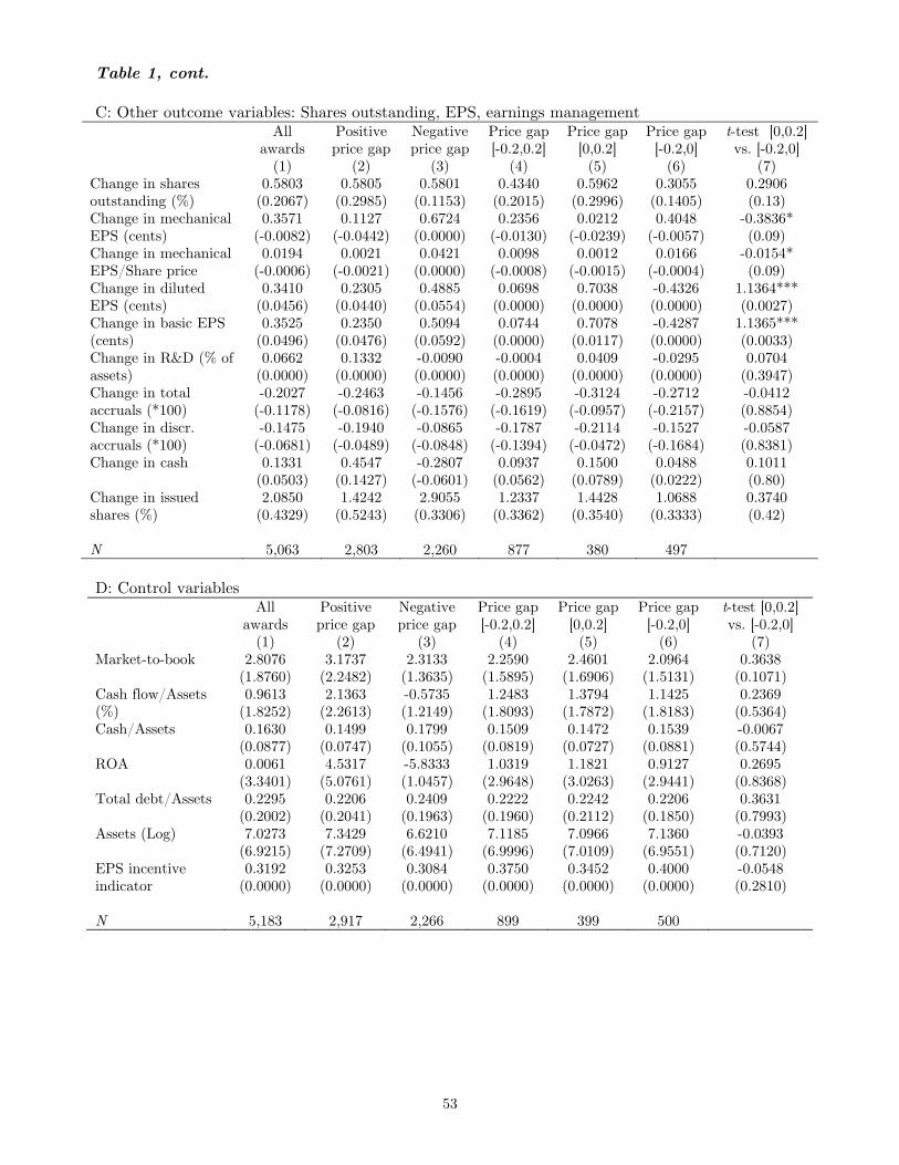
53

Table 1, cont. C: Other outcome variables: Shares outstanding, EPS, earnings management

All awards

Positive price gap

Negative price gap

Price gap [-0.2,0.2]

Price gap [0,0.2]

Price gap [-0.2,0]

t-test [0,0.2] vs. [-0.2,0]

(1) (2) (3) (4) (5) (6) (7) Change in shares outstanding (%)

0.5803 0.5805 0.5801 0.4340 0.5962 0.3055 0.2906 (0.2067) (0.2985) (0.1153) (0.2015) (0.2996) (0.1405) (0.13)

Change in mechanical EPS (cents)

0.3571 0.1127 0.6724 0.2356 0.0212 0.4048 -0.3836* (-0.0082) (-0.0442) (0.0000) (-0.0130) (-0.0239) (-0.0057) (0.09)

Change in mechanical EPS/Share price

0.0194 0.0021 0.0421 0.0098 0.0012 0.0166 -0.0154* (-0.0006) (-0.0021) (0.0000) (-0.0008) (-0.0015) (-0.0004) (0.09)

Change in diluted EPS (cents)

0.3410 0.2305 0.4885 0.0698 0.7038 -0.4326 1.1364*** (0.0456) (0.0440) (0.0554) (0.0000) (0.0000) (0.0000) (0.0027)

Change in basic EPS (cents)

0.3525 0.2350 0.5094 0.0744 0.7078 -0.4287 1.1365*** (0.0496) (0.0476) (0.0592) (0.0000) (0.0117) (0.0000) (0.0033)

Change in R&D (% of assets)

0.0662 0.1332 -0.0090 -0.0004 0.0409 -0.0295 0.0704 (0.0000) (0.0000) (0.0000) (0.0000) (0.0000) (0.0000) (0.3947)

Change in total accruals (*100)

-0.2027 -0.2463 -0.1456 -0.2895 -0.3124 -0.2712 -0.0412 (-0.1178) (-0.0816) (-0.1576) (-0.1619) (-0.0957) (-0.2157) (0.8854)

Change in discr. accruals (*100)

-0.1475 -0.1940 -0.0865 -0.1787 -0.2114 -0.1527 -0.0587 (-0.0681) (-0.0489) (-0.0848) (-0.1394) (-0.0472) (-0.1684) (0.8381)

Change in cash 0.1331 (0.0503)

0.4547 (0.1427)

-0.2807 (-0.0601)

0.0937 (0.0562)

0.1500 (0.0789)

0.0488 (0.0222)

0.1011 (0.80)

Change in issued shares (%)

2.0850 (0.4329)

1.4242 (0.5243)

2.9055 (0.3306)

1.2337 (0.3362)

1.4428 (0.3540)

1.0688 (0.3333)

0.3740 (0.42)

N 5,063 2,803 2,260 877 380 497 D: Control variables All

awards Positive price gap

Negative price gap

Price gap [-0.2,0.2]

Price gap [0,0.2]

Price gap [-0.2,0]

t-test [0,0.2] vs. [-0.2,0]

(1) (2) (3) (4) (5) (6) (7) Market-to-book 2.8076 3.1737 2.3133 2.2590 2.4601 2.0964 0.3638

(1.8760) (2.2482) (1.3635) (1.5895) (1.6906) (1.5131) (0.1071) Cash flow/Assets (%)

0.9613 2.1363 -0.5735 1.2483 1.3794 1.1425 0.2369 (1.8252) (2.2613) (1.2149) (1.8093) (1.7872) (1.8183) (0.5364)

Cash/Assets 0.1630 0.1499 0.1799 0.1509 0.1472 0.1539 -0.0067 (0.0877) (0.0747) (0.1055) (0.0819) (0.0727) (0.0881) (0.5744)

ROA 0.0061 4.5317 -5.8333 1.0319 1.1821 0.9127 0.2695 (3.3401) (5.0761) (1.0457) (2.9648) (3.0263) (2.9441) (0.8368)

Total debt/Assets 0.2295 0.2206 0.2409 0.2222 0.2242 0.2206 0.3631 (0.2002) (0.2041) (0.1963) (0.1960) (0.2112) (0.1850) (0.7993)

Assets (Log) 7.0273 7.3429 6.6210 7.1185 7.0966 7.1360 -0.0393 (6.9215) (7.2709) (6.4941) (6.9996) (7.0109) (6.9551) (0.7120)

EPS incentive indicator

0.3192 0.3253 0.3084 0.3750 0.3452 0.4000 -0.0548 (0.0000) (0.0000) (0.0000) (0.0000) (0.0000) (0.0000) (0.2810)

N 5,183 2,917 2,266 899 399 500

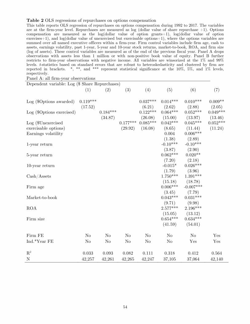
54

Table 2 OLS regressions of repurchases on options compensation This table reports OLS regression of repurchases on options compensation during 1992 to 2017. The variables are at the firm-year level. Repurchases are measured as log (dollar value of share repurchase +1). Options compensation are measured as the log(dollar value of option grants+1), log(dollar value of option exercises+1), and log(dollar value of unexercised but exercisable options+1), where the options variables are summed over all named executive officers within a firm-year. Firm control variables include firm age, cash to assets, earnings volatility, past 1-year, 5-year and 10-year stock returns, market-to-book, ROA, and firm size (log of assets). These control variables are measured as of the end of the previous fiscal year. Panel A drops observations with assets less than 1 million or with non-positive book value of equity. Panel B further restricts to firm-year observations with negative income. All variables are winsorized at the 1% and 99% levels. t-statistics based on standard errors that are robust to heteroskedasticity and clustered by firm are reported in brackets. *, **, and *** represent statistical significance at the 10%, 5%, and 1% levels, respectively. Panel A: all firm-year observations Dependent variable: Log ($ Share Repurchases) (1) (2) (3) (4) (5) (6) (7) Log ($Options awarded) 0.119***

(17.52) 0.037***

(6.21) 0.014*** (2.62)

0.010*** (2.88)

0.009** (2.05)

Log ($Options exercised) 0.184*** (34.87)

0.122*** (26.08)

0.064*** (15.00)

0.052*** (13.97)

0.049*** (13.46)

Log ($Unexercised exercisable options)

0.177*** (29.92)

0.085*** (16.08)

0.042*** (8.65)

0.045*** (11.44)

0.052*** (11.24)

Earnings volatility 0.004 (1.38)

0.006*** (2.89)

1-year return -0.10*** (3.87)

-0.10*** (2.90)

5-year return 0.062*** (7.20)

0.020** (2.18)

10-year return -0.015* (1.79)

0.026*** (3.96)

Cash/Assets 1.750*** (15.18)

1.391*** (18.78)

Firm age 0.006*** (3.45)

-0.007*** (7.79)

Market-to-book 0.043*** (9.71)

0.031*** (9.98)

ROA 2.577*** (15.05)

2.196*** (13.12)

Firm size 0.654*** (41.59)

0.634*** (54.01)

Firm FE No No No No No No Yes Ind.*Year FE No No No No No Yes Yes R2 0.033 0.093 0.082 0.111 0.318 0.412 0.564 N 42,257 42,261 42,265 42,247 37,105 37,064 42,140

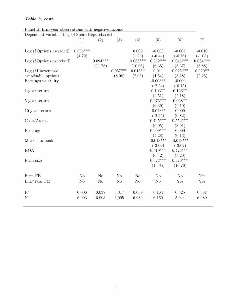
55

Table 2, cont. Panel B: firm-year observations with negative income Dependent variable: Log ($ Share Repurchases) (1) (2) (3) (4) (5) (6) (7) Log ($Options awarded) 0.035***

(4.79) 0.009

(1.23) -0.003 (-0.44)

-0.006 (-0.76)

-0.010 (-1.08)

Log ($Options exercised) 0.094*** (11.75)

0.083*** (10.05)

0.052*** (6.35)

0.045*** (5.37)

0.034*** (3.88)

Log ($Unexercised exercisable options)

0.057*** (8.08)

0.015** (2.05)

0.011 (1.54)

0.025*** (3.28)

0.020** (2.25)

Earnings volatility -0.003** (-2.24)

-0.000 (-0.15)

1-year return 0.103** (2.51)

0.126** (2.18)

5-year return 0.073*** (6.39)

0.028** (2.10)

10-year return -0.023** (-2.25)

0.009 (0.82)

Cash/Assets 0.745*** (6.05)

0.552*** (3.91)

Firm age 0.009*** (4.28)

0.000 (0.13)

Market-to-book -0.013*** (-3.00)

-0.013*** (-3.02)

ROA 0.519*** (6.42)

0.426*** (5.20)

Firm size 0.323*** (16.35)

0.320*** (16.76)

Firm FE No No No No No No Yes Ind.*Year FE No No No No No Yes Yes R2 0.006 0.037 0.017 0.039 0.164 0.325 0.587 N 6,993 6,993 6,995 6,989 6,160 5,944 6,089

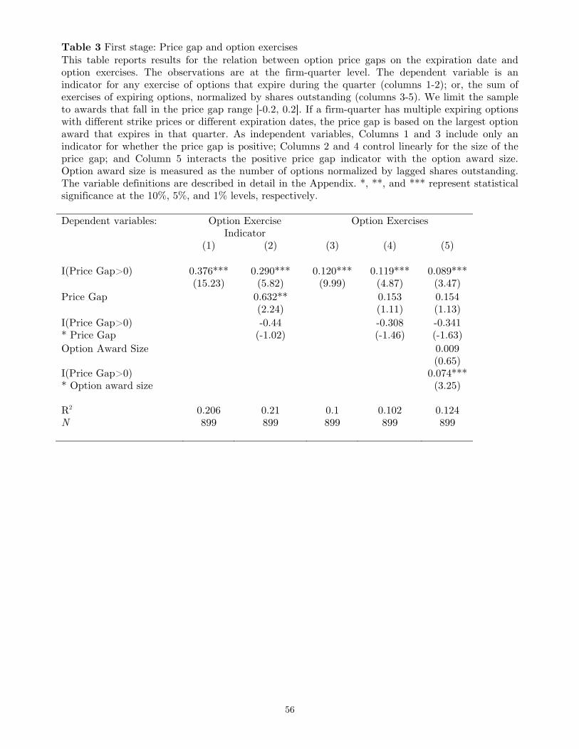
56

Table 3 First stage: Price gap and option exercises This table reports results for the relation between option price gaps on the expiration date and option exercises. The observations are at the firm-quarter level. The dependent variable is an indicator for any exercise of options that expire during the quarter (columns 1-2); or, the sum of exercises of expiring options, normalized by shares outstanding (columns 3-5). We limit the sample to awards that fall in the price gap range [-0.2, 0.2]. If a firm-quarter has multiple expiring options with different strike prices or different expiration dates, the price gap is based on the largest option award that expires in that quarter. As independent variables, Columns 1 and 3 include only an indicator for whether the price gap is positive; Columns 2 and 4 control linearly for the size of the price gap; and Column 5 interacts the positive price gap indicator with the option award size. Option award size is measured as the number of options normalized by lagged shares outstanding. The variable definitions are described in detail in the Appendix. *, **, and *** represent statistical significance at the 10%, 5%, and 1% levels, respectively. Dependent variables: Option Exercise

Indicator Option Exercises

(1) (2) (3) (4) (5) I(Price Gap>0) 0.376***

(15.23) 0.290*** (5.82)

0.120*** (9.99)

0.119*** (4.87)

0.089*** (3.47)

Price Gap 0.632** (2.24)

0.153 (1.11)

0.154 (1.13)

I(Price Gap>0) * Price Gap

-0.44 (-1.02)

-0.308 (-1.46)

-0.341 (-1.63)

Option Award Size 0.009 (0.65)

I(Price Gap>0) * Option award size

0.074*** (3.25)

R2 0.206 0.21 0.1 0.102 0.124 N 899 899 899 899 899

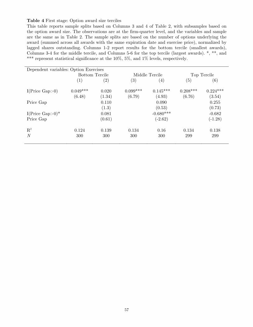
57

Table 4 First stage: Option award size terciles This table reports sample splits based on Columns 3 and 4 of Table 2, with subsamples based on the option award size. The observations are at the firm-quarter level, and the variables and sample are the same as in Table 2. The sample splits are based on the number of options underlying the award (summed across all awards with the same expiration date and exercise price), normalized by lagged shares outstanding. Columns 1-2 report results for the bottom tercile (smallest awards), Columns 3-4 for the middle tercile, and Columns 5-6 for the top tercile (largest awards). *, **, and *** represent statistical significance at the 10%, 5%, and 1% levels, respectively. Dependent variables: Option Exercises Bottom Tercile Middle Tercile Top Tercile (1) (2) (3) (4) (5) (6) I(Price Gap>0) 0.049***

(6.48) 0.020 (1.34)

0.099*** (6.79)

0.145*** (4.93)

0.208*** (6.76)

0.224*** (3.54)

Price Gap 0.110 (1.3)

0.090 (0.53)

0.255 (0.73)

I(Price Gap>0)* Price Gap

0.081 (0.61)

-0.680*** (-2.62)

-0.682 (-1.28)

R2 0.124 0.139 0.134 0.16 0.134 0.138 N 300 300 300 300 299 299

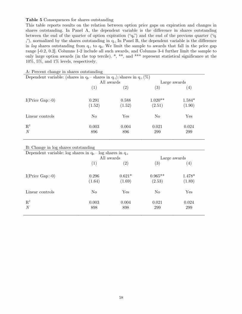
58

Table 5 Consequences for shares outstanding This table reports results on the relation between option price gaps on expiration and changes in shares outstanding. In Panel A, the dependent variable is the difference in shares outstanding between the end of the quarter of option expiration (“q0”) and the end of the previous quarter (“q-

1”), normalized by the shares outstanding in q-1. In Panel B, the dependent variable is the difference in log shares outstanding from q-1 to q0. We limit the sample to awards that fall in the price gap range [-0.2, 0.2]. Columns 1-2 include all such awards, and Columns 3-4 further limit the sample to only large option awards (in the top tercile). *, **, and *** represent statistical significance at the 10%, 5%, and 1% levels, respectively. A: Percent change in shares outstanding Dependent variable: (shares in q0 – shares in q-1)/shares in q-1 (%) All awards Large awards (1) (2) (3) (4) I(Price Gap>0) 0.291

(1.52) 0.588 (1.52)

1.020** (2.51)

1.584* (1.90)

Linear controls No Yes No Yes R2 0.003 0.004 0.021 0.024 N 896 896 299 299 B: Change in log shares outstanding Dependent variable: log shares in q0 – log shares in q-1 All awards Large awards (1) (2) (3) (4) I(Price Gap>0) 0.296

(1.64) 0.621* (1.69)

0.965** (2.53)

1.478* (1.89)

Linear controls No Yes No Yes R2 0.003 0.004 0.021 0.024 N 898 898 299 299

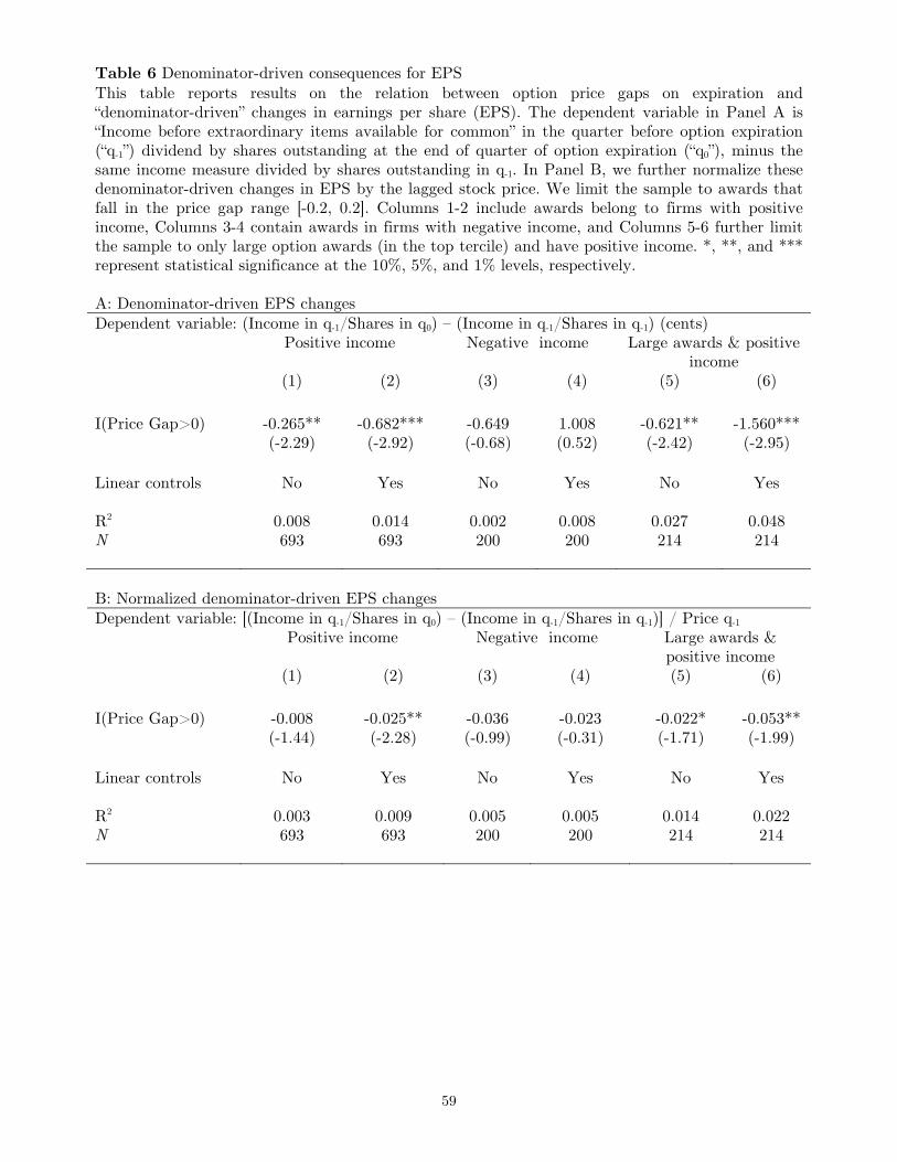
59

Table 6 Denominator-driven consequences for EPS This table reports results on the relation between option price gaps on expiration and “denominator-driven” changes in earnings per share (EPS). The dependent variable in Panel A is “Income before extraordinary items available for common” in the quarter before option expiration (“q-1”) dividend by shares outstanding at the end of quarter of option expiration (“q0”), minus the same income measure divided by shares outstanding in q-1. In Panel B, we further normalize these denominator-driven changes in EPS by the lagged stock price. We limit the sample to awards that fall in the price gap range [-0.2, 0.2]. Columns 1-2 include awards belong to firms with positive income, Columns 3-4 contain awards in firms with negative income, and Columns 5-6 further limit the sample to only large option awards (in the top tercile) and have positive income. *, **, and *** represent statistical significance at the 10%, 5%, and 1% levels, respectively. A: Denominator-driven EPS changes Dependent variable: (Income in q-1/Shares in q0) – (Income in q-1/Shares in q-1) (cents) Positive income Negative income Large awards & positive

income (1) (2) (3) (4) (5) (6) I(Price Gap>0) -0.265**

(-2.29) -0.682*** (-2.92)

-0.649 (-0.68)

1.008 (0.52)

-0.621** (-2.42)

-1.560*** (-2.95)

Linear controls No Yes No Yes No Yes R2 0.008 0.014 0.002 0.008 0.027 0.048 N 693 693 200 200 214 214 B: Normalized denominator-driven EPS changes Dependent variable: [(Income in q-1/Shares in q0) – (Income in q-1/Shares in q-1)] / Price q-1 Positive income Negative income Large awards &

positive income (1) (2) (3) (4) (5) (6) I(Price Gap>0) -0.008

(-1.44) -0.025** (-2.28)

-0.036 (-0.99)

-0.023 (-0.31)

-0.022* (-1.71)

-0.053** (-1.99)

Linear controls No Yes No Yes No Yes R2 0.003 0.009 0.005 0.005 0.014 0.022 N 693 693 200 200 214 214

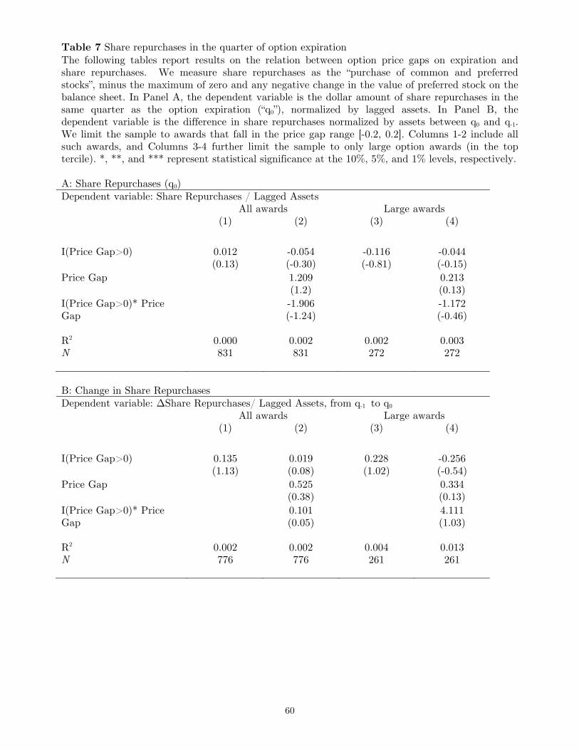
60

Table 7 Share repurchases in the quarter of option expiration The following tables report results on the relation between option price gaps on expiration and share repurchases. We measure share repurchases as the “purchase of common and preferred stocks”, minus the maximum of zero and any negative change in the value of preferred stock on the balance sheet. In Panel A, the dependent variable is the dollar amount of share repurchases in the same quarter as the option expiration (“q0”), normalized by lagged assets. In Panel B, the dependent variable is the difference in share repurchases normalized by assets between q0 and q-1. We limit the sample to awards that fall in the price gap range [-0.2, 0.2]. Columns 1-2 include all such awards, and Columns 3-4 further limit the sample to only large option awards (in the top tercile). *, **, and *** represent statistical significance at the 10%, 5%, and 1% levels, respectively. A: Share Repurchases (q0) Dependent variable: Share Repurchases / Lagged Assets All awards Large awards (1) (2) (3) (4) I(Price Gap>0) 0.012

(0.13) -0.054 (-0.30)

-0.116 (-0.81)

-0.044 (-0.15)

Price Gap 1.209 (1.2)

0.213 (0.13)

I(Price Gap>0)* Price Gap

-1.906 (-1.24)

-1.172 (-0.46)

R2 0.000 0.002 0.002 0.003 N 831 831 272 272 B: Change in Share Repurchases Dependent variable: ∆Share Repurchases/ Lagged Assets, from q-1 to q0 All awards Large awards (1) (2) (3) (4) I(Price Gap>0) 0.135

(1.13) 0.019 (0.08)

0.228 (1.02)

-0.256 (-0.54)

Price Gap 0.525 (0.38)

0.334 (0.13)

I(Price Gap>0)* Price Gap

0.101 (0.05)

4.111 (1.03)

R2 0.002 0.002 0.004 0.013 N 776 776 261 261

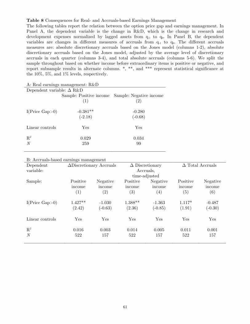
61

Table 8 Consequences for Real- and Accruals-based Earnings Management The following tables report the relation between the option price gap and earnings management. In Panel A, the dependent variable is the change in R&D, which is the change in research and development expenses normalized by lagged assets from q-1 to q0. In Panel B, the dependent variables are changes in different measures of accruals from q-1 to q0. The different accruals measures are: absolute discretionary accruals based on the Jones model (columns 1-2), absolute discretionary accruals based on the Jones model, adjusted by the average level of discretionary accruals in each quarter (columns 3-4), and total absolute accruals (columns 5-6). We split the sample throughout based on whether income before extraordinary items is positive or negative, and report subsample results in alternate columns. *, **, and *** represent statistical significance at the 10%, 5%, and 1% levels, respectively. A: Real earnings management: R&D Dependent variable: ∆ R&D Sample: Positive income Sample: Negative income (1) (2) I(Price Gap>0) -0.381**

(-2.18) -0.280 (-0.68)

Linear controls Yes Yes R2 0.029 0.034 N 259 99 B: Accruals-based earnings management Dependent variable:

∆Discretionary Accruals ∆ Discretionary Accruals,

time-adjusted

∆ Total Accruals

Sample: Positive income

Negative income

Positive income

Negative income

Positive income

Negative income

(1) (2) (3) (4) (5) (6) I(Price Gap>0) 1.427**

(2.42) -1.030 (-0.63)

1.388** (2.36)

-1.363 (-0.85)

1.117* (1.91)

-0.487 (-0.30)

Linear controls Yes Yes Yes Yes Yes Yes R2 0.016 0.003 0.014 0.005 0.011 0.001 N 522 157 522 157 522 157

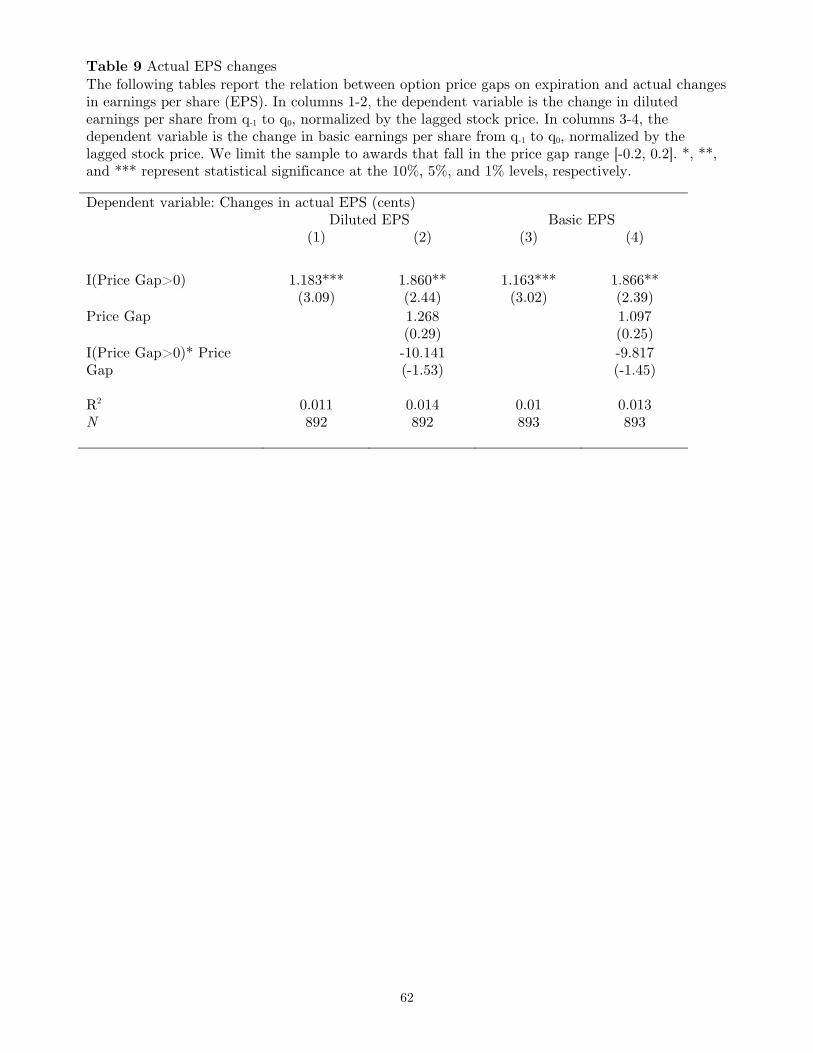
62

Table 9 Actual EPS changes The following tables report the relation between option price gaps on expiration and actual changes in earnings per share (EPS). In columns 1-2, the dependent variable is the change in diluted earnings per share from q-1 to q0, normalized by the lagged stock price. In columns 3-4, the dependent variable is the change in basic earnings per share from q-1 to q0, normalized by the lagged stock price. We limit the sample to awards that fall in the price gap range [-0.2, 0.2]. *, **, and *** represent statistical significance at the 10%, 5%, and 1% levels, respectively.

Dependent variable: Changes in actual EPS (cents) Diluted EPS Basic EPS (1) (2) (3) (4) I(Price Gap>0) 1.183***

(3.09) 1.860** (2.44)

1.163*** (3.02)

1.866** (2.39)

Price Gap 1.268 (0.29)

1.097 (0.25)

I(Price Gap>0)* Price Gap

-10.141 (-1.53)

-9.817 (-1.45)

R2 0.011 0.014 0.01 0.013 N 892 892 893 893

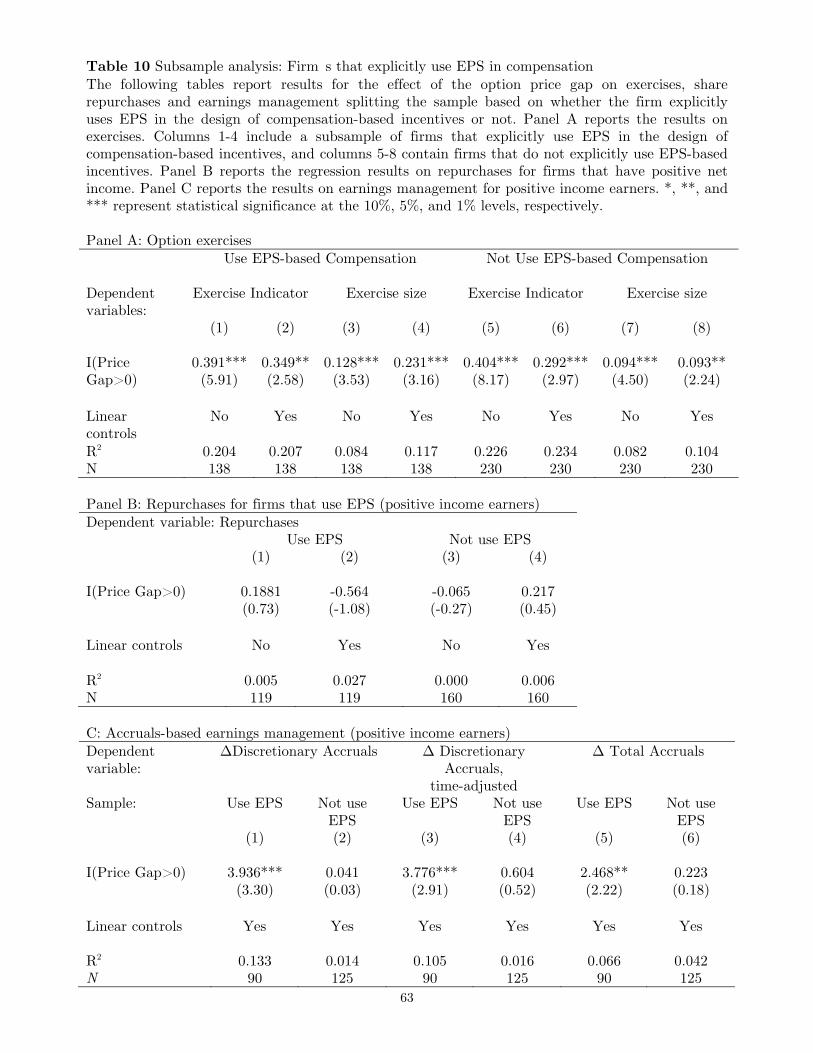
63

Table 10 Subsample analysis: Firm s that explicitly use EPS in compensation The following tables report results for the effect of the option price gap on exercises, share repurchases and earnings management splitting the sample based on whether the firm explicitly uses EPS in the design of compensation-based incentives or not. Panel A reports the results on exercises. Columns 1-4 include a subsample of firms that explicitly use EPS in the design of compensation-based incentives, and columns 5-8 contain firms that do not explicitly use EPS-based incentives. Panel B reports the regression results on repurchases for firms that have positive net income. Panel C reports the results on earnings management for positive income earners. *, **, and *** represent statistical significance at the 10%, 5%, and 1% levels, respectively. Panel A: Option exercises Use EPS-based Compensation Not Use EPS-based Compensation Dependent variables:

Exercise Indicator Exercise size Exercise Indicator Exercise size

(1) (2) (3) (4) (5) (6) (7) (8) I(Price Gap>0)

0.391*** (5.91)

0.349** (2.58)

0.128*** (3.53)

0.231*** (3.16)

0.404*** (8.17)

0.292*** (2.97)

0.094*** (4.50)

0.093** (2.24)

Linear controls

No Yes No Yes No Yes No Yes

R2 0.204 0.207 0.084 0.117 0.226 0.234 0.082 0.104 N 138 138 138 138 230 230 230 230 Panel B: Repurchases for firms that use EPS (positive income earners) Dependent variable: Repurchases Use EPS Not use EPS (1) (2) (3) (4) I(Price Gap>0) 0.1881

(0.73) -0.564 (-1.08)

-0.065 (-0.27)

0.217 (0.45)

Linear controls No Yes No Yes R2 0.005 0.027 0.000 0.006 N 119 119 160 160 C: Accruals-based earnings management (positive income earners) Dependent variable:

∆Discretionary Accruals ∆ Discretionary Accruals,

time-adjusted

∆ Total Accruals

Sample: Use EPS Not use EPS

Use EPS Not use EPS

Use EPS Not use EPS

(1) (2) (3) (4) (5) (6) I(Price Gap>0) 3.936***

(3.30) 0.041 (0.03)

3.776*** (2.91)

0.604 (0.52)

2.468** (2.22)

0.223 (0.18)

Linear controls Yes Yes Yes Yes Yes Yes R2 0.133 0.014 0.105 0.016 0.066 0.042 N 90 125 90 125 90 125

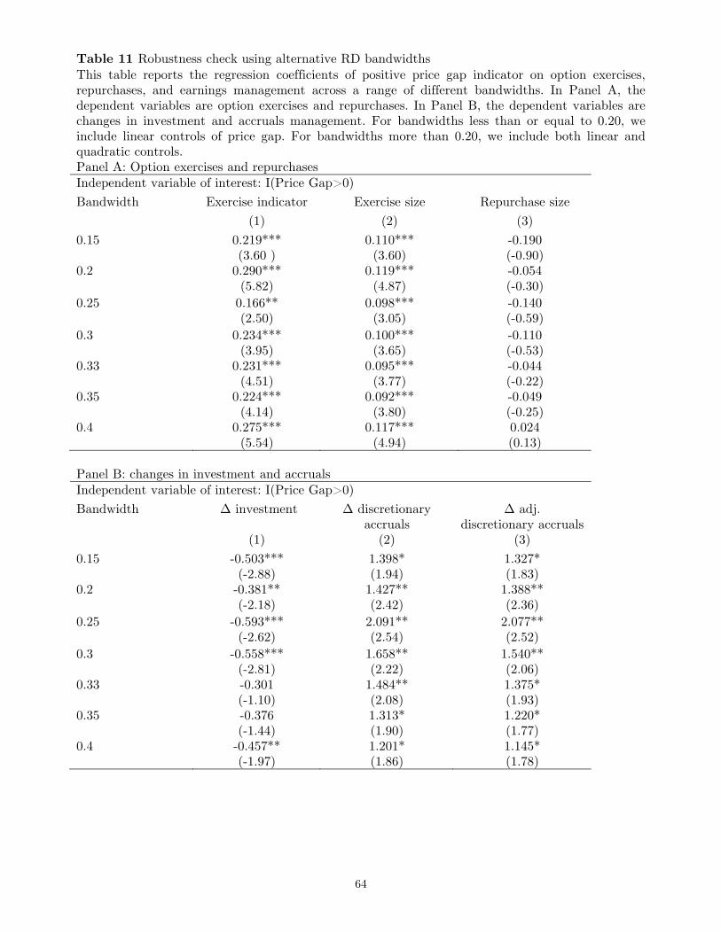
64

Table 11 Robustness check using alternative RD bandwidths This table reports the regression coefficients of positive price gap indicator on option exercises, repurchases, and earnings management across a range of different bandwidths. In Panel A, the dependent variables are option exercises and repurchases. In Panel B, the dependent variables are changes in investment and accruals management. For bandwidths less than or equal to 0.20, we include linear controls of price gap. For bandwidths more than 0.20, we include both linear and quadratic controls. Panel A: Option exercises and repurchases Independent variable of interest: I(Price Gap>0) Bandwidth Exercise indicator Exercise size Repurchase size (1) (2) (3) 0.15

0.219*** (3.60 )

0.110*** (3.60)

-0.190 (-0.90)

0.2 0.290*** (5.82)

0.119*** (4.87)

-0.054 (-0.30)

0.25 0.166** (2.50)

0.098*** (3.05)

-0.140 (-0.59)

0.3 0.234*** (3.95)

0.100*** (3.65)

-0.110 (-0.53)

0.33

0.231*** (4.51)

0.095*** (3.77)

-0.044 (-0.22)

0.35 0.224*** (4.14)

0.092*** (3.80)

-0.049 (-0.25)

0.4 0.275*** (5.54)

0.117*** (4.94)

0.024 (0.13)

Panel B: changes in investment and accruals Independent variable of interest: I(Price Gap>0) Bandwidth ∆ investment ∆ discretionary

accruals ∆ adj.

discretionary accruals (1) (2) (3) 0.15

-0.503*** (-2.88)

1.398* (1.94)

1.327* (1.83)

0.2 -0.381** (-2.18)

1.427** (2.42)

1.388** (2.36)

0.25 -0.593*** (-2.62)

2.091** (2.54)

2.077** (2.52)

0.3 -0.558*** (-2.81)

1.658** (2.22)

1.540** (2.06)

0.33

-0.301 (-1.10)

1.484** (2.08)

1.375* (1.93)

0.35 -0.376 (-1.44)

1.313* (1.90)

1.220* (1.77)

0.4 -0.457** (-1.97)

1.201* (1.86)

1.145* (1.78)

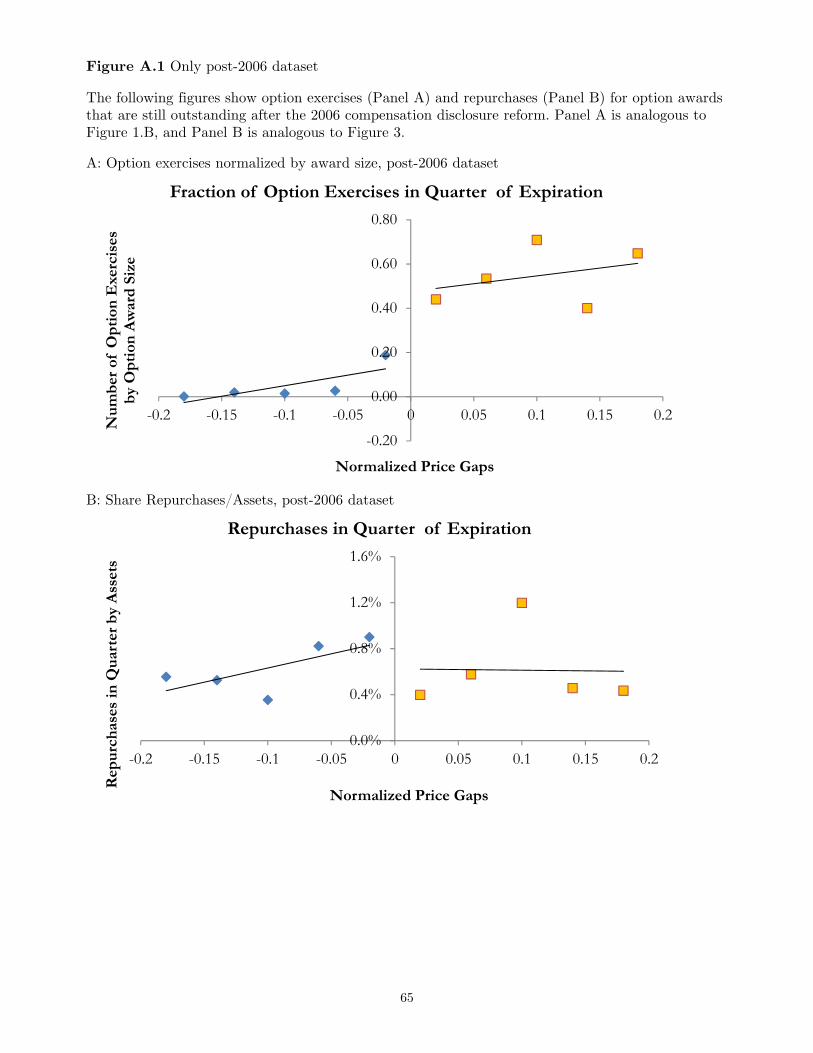
65

Figure A.1 Only post-2006 dataset

The following figures show option exercises (Panel A) and repurchases (Panel B) for option awards that are still outstanding after the 2006 compensation disclosure reform. Panel A is analogous to Figure 1.B, and Panel B is analogous to Figure 3.

A: Option exercises normalized by award size, post-2006 dataset

B: Share Repurchases/Assets, post-2006 dataset

-0.20

0.00

0.20

0.40

0.60

0.80

-0.2 -0.15 -0.1 -0.05 0 0.05 0.1 0.15 0.2

Nu

mb

er o

f O

pti

on E

xerc

ises

b

y O

pti

on A

war

d S

ize

Normalized Price Gaps

Fraction of Option Exercises in Quarter of Expiration

0.0%

0.4%

0.8%

1.2%

1.6%

-0.2 -0.15 -0.1 -0.05 0 0.05 0.1 0.15 0.2

Rep

urc

has

es in

Qu

arte

r b

y A

sset

s

Normalized Price Gaps

Repurchases in Quarter of Expiration

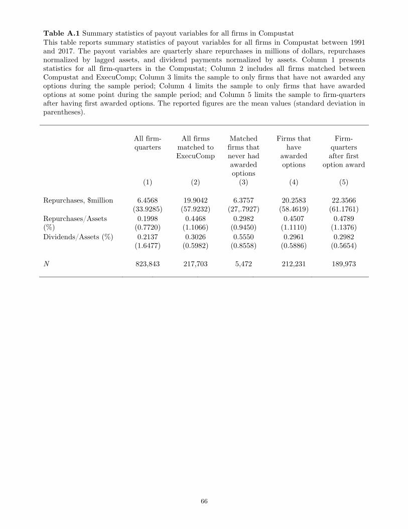
66

Table A.1 Summary statistics of payout variables for all firms in Compustat This table reports summary statistics of payout variables for all firms in Compustat between 1991 and 2017. The payout variables are quarterly share repurchases in millions of dollars, repurchases normalized by lagged assets, and dividend payments normalized by assets. Column 1 presents statistics for all firm-quarters in the Compustat; Column 2 includes all firms matched between Compustat and ExecuComp; Column 3 limits the sample to only firms that have not awarded any options during the sample period; Column 4 limits the sample to only firms that have awarded options at some point during the sample period; and Column 5 limits the sample to firm-quarters after having first awarded options. The reported figures are the mean values (standard deviation in parentheses). All firm-

quarters All firms

matched to ExecuComp

Matched firms that never had awarded options

Firms that have

awarded options

Firm-quarters after first

option award

(1) (2) (3) (4) (5)

Repurchases, $million 6.4568 (33.9285)

19.9042 (57.9232)

6.3757 (27,.7927)

20.2583 (58.4619)

22.3566 (61.1761)

Repurchases/Assets (%)

0.1998 (0.7720)

0.4468 (1.1066)

0.2982 (0.9450)

0.4507 (1.1110)

0.4789 (1.1376)

Dividends/Assets (%) 0.2137 (1.6477)

0.3026 (0.5982)

0.5550 (0.8558)

0.2961 (0.5886)

0.2982 (0.5654)

N 823,843 217,703 5,472 212,231 189,973

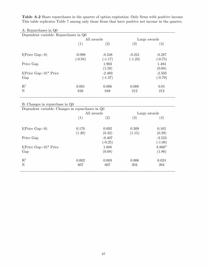
67

Table A.2 Share repurchases in the quarter of option expiration: Only firms with positive income This table replicates Table 7 among only those firms that have positive net income in the quarter. A: Repurchases in Q0 Dependent variable: Repurchases in Q0 All awards Large awards (1) (2) (3) (4) I(Price Gap>0) -0.098

(-0.94) -0.248 (-1.17)

-0.221 (-1.23)

-0.287 (-0.75)

Price Gap 1.903 (1.59)

1.484 (0.68)

I(Price Gap>0)* Price Gap

-2.493 (-1.37)

-2.503 (-0.79)

R2 0.001 0.006 0.008 0.01 N 648 648 212 212 B: Changes in repurchase in Q0 Dependent variable: Changes in repurchases in Q0 All awards Large awards (1) (2) (3) (4) I(Price Gap>0) 0.170

(1.20) 0.092 (0.32)

0.309 (1.15)

0.165 (0.29)

Price Gap -0.407 (-0.25)

-3.523 (-1.08)

I(Price Gap>0)* Price Gap

1.688 (0.68)

8.866* (1.86)

R2 0.002 0.003 0.006 0.024 N 607 607 204 204

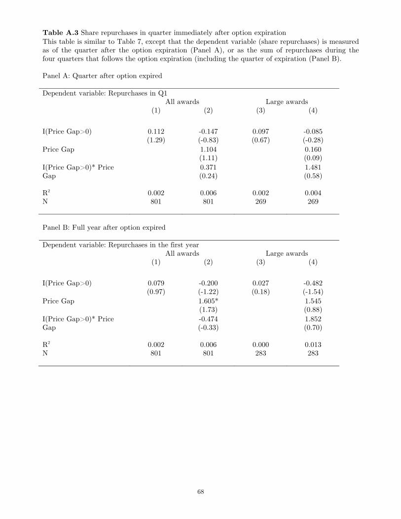
68

Table A.3 Share repurchases in quarter immediately after option expiration This table is similar to Table 7, except that the dependent variable (share repurchases) is measured as of the quarter after the option expiration (Panel A), or as the sum of repurchases during the four quarters that follows the option expiration (including the quarter of expiration (Panel B). Panel A: Quarter after option expired Dependent variable: Repurchases in Q1 All awards Large awards (1) (2) (3) (4) I(Price Gap>0) 0.112

(1.29) -0.147 (-0.83)

0.097 (0.67)

-0.085 (-0.28)

Price Gap 1.104 (1.11)

0.160 (0.09)

I(Price Gap>0)* Price Gap

0.371 (0.24)

1.481 (0.58)

R2 0.002 0.006 0.002 0.004 N 801 801 269 269 Panel B: Full year after option expired Dependent variable: Repurchases in the first year All awards Large awards (1) (2) (3) (4) I(Price Gap>0) 0.079

(0.97) -0.200 (-1.22)

0.027 (0.18)

-0.482 (-1.54)

Price Gap 1.605* (1.73)

1.545 (0.88)

I(Price Gap>0)* Price Gap

-0.474 (-0.33)

1.852 (0.70)

R2 0.002 0.006 0.000 0.013 N 801 801 283 283

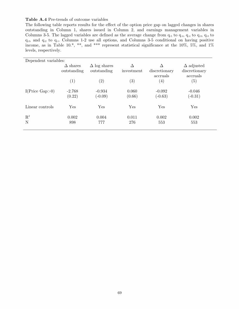
69

Table A.4 Pre-trends of outcome variables The following table reports results for the effect of the option price gap on lagged changes in shares outstanding in Column 1, shares issued in Column 2, and earnings management variables in Columns 3-5. The lagged variables are defined as the average change from q-5 to q-4, q-4 to q-3, q-3 to q-2, and q-2 to q-1. Columns 1-2 use all options, and Columns 3-5 conditional on having positive income, as in Table 10.*, **, and *** represent statistical significance at the 10%, 5%, and 1% levels, respectively. Dependent variables: ∆ shares

outstanding ∆ log shares outstanding

∆ investment

∆ discretionary

accruals

∆ adjusted discretionary

accruals (1) (2) (3) (4) (5) I(Price Gap>0) -2.768

(0.22) -0.934 (-0.09)

0.060 (0.66)

-0.092 (-0.63)

-0.046 (-0.31)

Linear controls Yes Yes Yes Yes Yes R2 0.002 0.004 0.011 0.002 0.002 N 898 777 276 553 553