option contracts and renegotiation: a solution to the hold-up problem
TRANSCRIPT

RAND Journal of EconomicsVol. 26, No. 2, Summer 1995pp. 163-179
Option contracts and renegotiation: a solutionto the hold-up problem
Georg Noldeke*
and
Klaus M. Schmidt*
In this article, we analyze the canonical hold-up model of Hart and Moore under the
assumption that the courts can verih deliveq of the good by the seller. [t is shown that
no further renegotiation design is necessary to achieve the first best: simple option contracts,
which give the seller the right to take the delivery decision and specify payments depending
on whether delivery takes place, allow
and eflicient trade,
implementation of e~icient investment decisions
1. Introduction■ In a seminal article, Hart and Moore (1988) considered a buyer-seller relationshipwith observable but unverifiable investment decisions. They argued that contractual iri-completeness, due to nonverifiability of the relevant state of the world, combined withthe parties’ inability to prevent e-xpost renegotiation will lead to underinvestment in sucha classical hold-up problem. This result has attracted considerable attention because itseems to provide a theoretical foundation for the rapidly growing literature on incompletecontracts, which tries to explain economic institutions, such as the allocation of ownershiprights or the financial structure of the fiw, as second-best solutions to incentive problemsin a world in which comprehensive contracts cannot be written.
In this article, we argue that the underinvestment problem in the Hart-Moore modelcan be overcome if the parties can write simple option contracts. An option contract givesthe seller the right (but not the obligation) to deliver a fixed quantity of the good andmakes the buyer’s contractual payment contingent on the seller’s delivery decision. Notethat an option contract is feasible only if it is possible to enforce payments conditional onthe seller’s delivery decision, that is, the court must be able to observe whether the seller
* University of Bonn.An earlier version of this article was circulated under the title “Unverifiable Information, Incomplete
Contracts, and Renegotiation. ” We would like to thank Dieter Balkenborg, Frank Bickenbach, Oliver Hart,
Bengt Holmstr6m, Kai-Uwe Kuhn, Albert Ma, Bentley MacLeod, Benny Moldovanu, John Moore, MonikaSchnitzer, Urs Schweizer, two anonymous referees, and in particular Mike Riordan for helpful comments anddiscussions. This research was initiated during the International Summer School of the Center for the Study ofthe New Institutional Economics in Wallerfangen, Germany, August 1990. We are grateful to Professor RudolfRichter for providing this stimulating atmosphere. Financial support by Deutsche Forschungsgemeinschaft, SFB303 at the University of Bonn, is gratefully acknowledged.
Copyright 01995, RAND 163

164 / THE RAND JOURNAL OF ECONOMICS
delivered the good to the buyer. This possibility is explicitly ruled out by Hart and Moorewho assume that, if trade fails, a court cannot distinguish whether the seller refused tosupply or whether the buyer refused to take delivery. It is this assumption, and only thisassumption, from the original Hart-Moore model that we need to abandon in order toachieve the first best.
To put our contribution into perspective, it is useful to relate our results to Aghion,Dewatripont, and Rey (1994). These authors have shown that the underinvestment problemcan be solved if renegotiation design is possible, in the sense that the contractual envi-ronment allows (i) allocation of all bargaining power in the renegotiation game to one ofthe contracting parties and (ii) specification of an appropriate default point that obtains ifrenegotiation breaks down. The logic behind this result is that the party who has all thebargaining power in the renegotiation game becomes residual claimant on total surplus(minus a constant) and thus has the right incentives to invest. Incentives for the other partyare then provided through the effect his investment has on the value of the default point.In a second step, the authors present a model of the renegotiation process—quite differentfrom the one assumed by Hart and Moore—that achieves the required renegotiation designthrough the use of specific performance clauses and penalties for delay in the original contract. 1
In contrast to Aghion, Dewatripont, and Rey, Hart and Moore took the renegotiationprocess as exogenously given. We shall show that, given their renegotiation process, everyoption contract results in the allocation of all bargaining power to the buyer in the rene-gotiation game. Hence, property (i) obtains naturally and the buyer has the right incentivesto invest. Although all option contracts result in the same allocation of bargaining power,different option contracts will induce different default points for the renegotiation game.Because the seller has the right to decide whether to deliver, the (implicit) default pointfor renegotiation is given by whatever delivery decision the seller prefers to make underthe terms of the initial contract. We shall show that adjusting the option price (i. e., theadditional payment required from the buyer if the seller exercises his option to deliver)provides us with enough flexibility to achieve property (ii) and thus provide the seller withthe correct investment incentives. Because we use the same renegotiation game as Hartand Moore, our approach highlights that it is Hart and Moore’s assumption that the courtcannot observe whether the seller delivered the good that is crucial to the underinvestmentresult (and not the exogenously given renegotiation game). 2
In order to further contrast our analysis with Aghion, Dewatripont, and Rey, considerthe case in which the good to be traded is indivisible and at most one unit can be traded(which is the only case considered by Hart and Moore and also the focus of most of ourarticle). In this case, Aghion, Dewatripont, and Rey rely on explicit randomization toachieve the first best, whereas no such randomization is necessary with an option contract.Aghion, Dewatripont, and Rey proceed by designing a contract that gives all the bar-gaining power in their renegotiation game to one party, say, the buyer. The problem thenbecomes providing the seller with the correct incentives. If no trade is specified as a defaultpoint, the seller has no incentive to invest. If trade of one unit is specified as a default
‘ Chung (1991) also shows that the first best can be achieved if (i) and (ii) are satisfied. However, whereasAghion, Dewatripont, and Rey offer an explicit contract, which generates a renegotiation game satisfying (i)and (ii), Chung just assumes that these conditions are satisfied.
‘ Remarks to this effect can already be found in Aghion, Dewatripont, and Rey and Hermalin and Katz(1993). Hermalin and Katz do not elaborate the point. Aghimr, Dmvatripont, and Rey observe that it is possibleto allocate all bargaining power to one party in the original Hafi-Moore model by choosing the price differentialin the original contract appropriate y. so that the only element of renegotiation design lacking from their modelseems to be the ability to assign a default point different from no trade. This argument is incomplete in thatit ignores the fact that, once different default points are introduced in the Hart –Moore model, it may no longerbe the case that the price differential influences the distribution of bargaining power as in Hart and Moore.Indeed, [he price differential in an option contract has no effect on the distribution of bargaining power. Insteadit serves to shift the default point.

NOLDEKE AND SCHMIDT / 165
point, overinvestment will be induced if the probability that trade is efficient is less thanone. To avoid this underinvestment (overinvestment) problem, Aghion, Dewatripont, andRey propose that the initial contract should specify “trade with probability q“ as a defaultpoint, where q is chosen to provide just the right investment incentives for the seller. Ofcourse, this contract requires that the probability of trade would be enforced by a court ifrenegotiation fails.
Suppose now that the renegotiation process is the same as in Hart and Moore andconsider an option contract that gives the seller the right to supply the good at price p, ornot to supply and receive PO. In this case, it is always the seller who has to be convinced(through renegotiation) to take the efficient action. The renegotiation game used by Hartand Moore has the property that the buyer can bribe the seller to do the right thing bymaking him just indifferent bet ween trade and no trade. Thus, the buyer becomes residualclaimant on the margin and, as in Aghion, Dewatripont, and Rey, is induced to investefficiently. What about the seller? There are two possible default points of renegotiationthat determine his utility: If the difference between PI and PO is higher than his productioncost, the seller will enforce trade. If, however, the difference between p[ and p. is smallerthan his production cost, he will choose not to trade. Because the seller’s production costsare a random variable, by varying p i – PO, we can vary the probability of the two defaultpoints and give the seller, in expectation, just the right incentives to invest. The maindifficulty in showing this result is that, in contrast to Aghion, Dewatripont, and Rey, thereis a feedback effect from investment decisions to the (expected) default point induced byan option contract: The seller’s investment affects the distribution of his production costsand thus the probability that “trade at p I” arises as the default point of contract renegotiation.
Although in most of our article we deal with the case in which at most one unit ofan indivisible good can be traded, our main results can be generalized to the case in whichthere are different levels of quantity and/or quality from which to choose. In this case,an option contract specifies one particular specification of the good and a price to be paidif the seller chooses to deliver exactly this specification. If any other specification is de-livered (and the contract has not been renegotiated), the buyer is not required to pay morethan the base payment, which he would have to pay even if the seller delivered nothing.We provide a simple condition under which the first best can be implemented if such anoption contract is enforced by the courts. This condition is automatically satisfied if tradeis a zero-one decision. Our result is in stark contrast to the incomplete contracts literature(e.g., Grossman and Hart (1986)) which argues that contracts are incomplete because ofthe difficulty to specify in advance the good to be traded contingent on a complex stateof the world. Our result can be interpreted as showing that a contingent contract is oftennot necessary but that the first best can be achieved if it is possible to contract on at leastone specification.
There is a large and growing recent literature dealing with contractual remedies to thehold-up problem. Rogerson ( 1992) shows that sequential mechanisms from the implementationliterature can be used to achieve the first best under a variety of informational assumptions.However, these mechanisms are typically not renegotiation-proof. MacLeod and Malcom-son (1993) and Edlin and Reichelstein (1993) consider a hold-up problem with a differentrenegotiation game. They focus on the case in which only one party has to make a re-lationship-specific investment and show that simple contracts can achieve the first best inthis case. For some special cases, their results carry over if both parties have to invest. 3
‘ MacLeod and Matcomson (1993) show that the first best can be achieved if (i) investments are notrelationship specific but there is a switching cost or (ii) if investments are specific and there is an observablevariable that is correlated with the investment levels and that can be contracted upon. Edlin and Reichelstein(1993) can implement the first best if the effect of investments and the effect of the state of the world enterthe production costs of the seller (and the valuation of the buyer) in an additively separable manner.
166 I THE RAND JOURNAL OF ECONOMICS
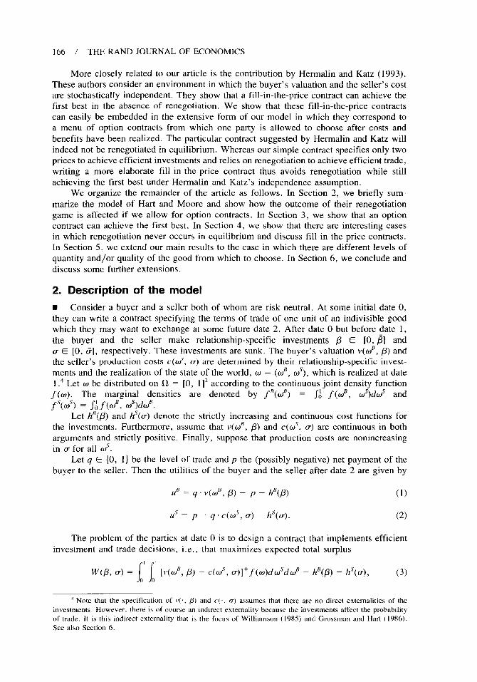
More closely related to our article is the contribution by Hermalin and Katz (1993).These authors consider an environment in which the buyer’s valuation and the seller’s costme stochastically independent. They show that a fill-in-the-price contract can achieve thefirst best in the absence of renegotiation. We show that these fill-in-the-price contractscan easily be embedded in the extensive form of our model in which they correspond toa menu of option contracts from which one party is allowed to choose after costs andbenefits have been realized. The particular contract suggested by Hermalin and Katz willindeed not be renegotiated in equilibrium. Whereas our simple contract specifies only twoprices to achieve efficient investments and relies on renegotiation to achieve efficient trade,writing a more elaborate fill-in-the-price contract thus avoids renegotiation while stillachieving the first best under Hermalin and Katz’s independence assumption.
We organize the remainder of the article as follows. In Section 2, we briefly sum-marize the model of Hart and Moore and show how the outcome of their renegotiationgame is affected if we allow for option contracts. In Section 3, we show that an optioncontract can achieve the first best. In Section 4, we show that there are interesting casesin which renegotiation never occurs in equilibrium and discuss fill-in-the-price contracts.In Section 5, we extend our main results to the case in which there are different levels ofquantity and/or quality of the good from which to choose. In Section 6, we conclude anddiscuss some further extensions.
2. Description of the model
8 Consider a buyer and a seller both of whom are risk neutral. At some initial date O,they can write a contract specifying the terms of trade of one unit of an indivisible goodwhich they may want to exchange at some future date 2. After date O but before date 1,the buyer and the seller make relationship-specific investments ~ c [0, ~] andu ~ [0, 6], respectively. These investments are sunk. The buyer’s valuation v(&, @) andthe seller’s production costs C(OJ’,u) are determined by their relationship-specific invest-ments and the realization of the state of the world, w = (w~, OS), which is realized at date1.4 Let w be distributed on Q = [0, 1]~ according to the continuous joint density function
f(w). The marginal densities are denoted by ~’(~e) = ~~ ~(w~, Ws)dOs and
f ‘(@s) = $i f (0’, ws)dco’.Let h~(~) and hs(cr) denote the strictly increasing and continuous cost functions for
the investments. Furthermore, assume that v(w~, ~) and C(tis, a) arc continuous in botharguments and strictly positive. Finally, suppose that production costs arc nonincreasingin m for all COs.
Let q E {O, 1} be the level of trade and p the (possibly negative) net payment of the
buyer to the seller. Then the utilities of the buyer and the seller after date 2 are given by
u“ = q . .((0’, /3) – p – h’(p) (1)
us = p – q.c(ti’, Cr) – /?’$(w). (2)
The problem of the parties at date O is to design a contract that implements efficientinvestment and trade decisions, i.e., that maximizes expected total surplus
.1 .1
HW(B,u) = [)’((0’, fl) - C(CIJ’,u)] ‘J”((o)dw’dtu’ - h’(p) - h’(tT), (3)00
‘ Note that the specification of v(., @ and C(,, a) assumes that there are no direct externalities of theinvestments. However, there is of course an indirect externality bccausc the investments affect the probabilityof trade. It is this indirect externality that is the focus of Williamson ( 1985) and Grossman and Hart ( 1986).See also Section 6.
NOLDEKE AND SCHMIDT I 167
where we shall frequently use the notation [o]+ = max{O, .} throughout the remainder ofthis article. Given our continuity assumptions, W(/3, @ is continuous in 13 and tr. Theboundedness assumption on ~ and u thus implies that the set of maximizers of W(, .)is always nonempty. Denote by (P*, o*) a pair of first-best investment levels thatmaximizes (3). For convenience, we assume that (B*, ~*) is unique. Also, let
Q’(o, P, 4 = w=m%{g” [V(OB, P) – C(OS, d]} denote the set of e.xpost efficient levelsof trade.
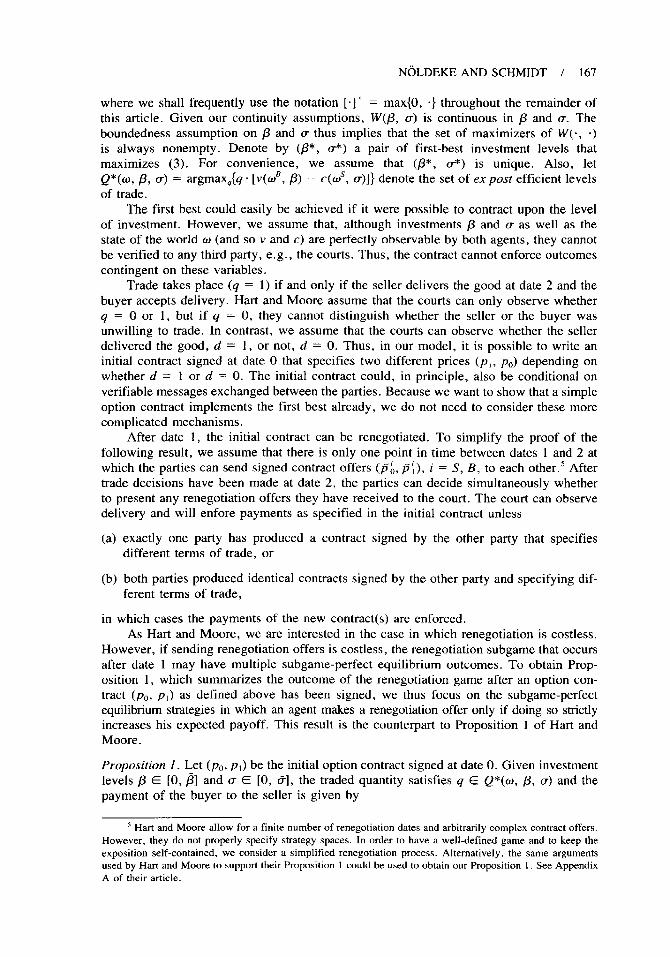
The first best could easily be achieved if it were possible to contract upon the levelof investment. However, we assume that, although investments ~ and ~ as well as thestate of the world o (and so v and c) are perfectly observable by both agents, they cannotbe verified to any third party, e.g., the courts. Thus, the contract cannot enforce outcomescontingent on these variables.
Trade takes place (q = 1) if and only if the seller delivers the good at date 2 and thebuyer accepts delivery. Hart and Moore assume that the courts can only observe whetherq = O or 1, but if q = O, they cannot distinguish whether the seller or the buyer wasunwilling to trade. In contrast, we assume that the courts can observe whether the sellerdelivered the good, d = 1, or not, d = O. Thus, in our model, it is possible to write aninitial contract signed at date O that specifies two different prices (p,, pO) depending onwhether d = 1 or d = O. The initial contract could, in principle, also be conditional onverifiable messages exchanged between the parties. Because we want to show that a simpleoption contract implements the first best already, we do not need to consider these morecomplicated mechanisms.
After date 1, the initial contract can be renegotiated. To simplify the proof of thefollowing result, we assume that there is only one point in time between dates 1 and 2 atwhich the parties can send signed contract offers (pi, p;), i = S, B, to each others Aftertrade decisions have been made at date 2, the parties can decide simultaneous y whetherto present any renegotiation offers they have received to the court. The court can observedelivery and will enfore payments as specified in the initial contract unless
(a)
(b)
exactly one party has produced a contract signed by the other party that specifiesdifferent terms of trade, or
both parties produced identical contracts signed by the other party and specifying dif-ferent terms of trade,
in which cases the payments of the new contract(s) are enforced.As Hart and Moore, we are interested in the case in which renegotiation is costless.
However, if sending renegotiation offers is costless, the renegotiation subgame that occursafter date 1 may have multiple subgame-perfect equilibrium outcomes. To obtain Prop-osition 1, which summarizes the outcome of the renegotiation game after an option con-tract (PO, p,) as defined above has been signed, we thus focus on the subgame-perfectequilibrium strategies in which an agent makes a renegotiation offer only if doing so strictlyincreases his expected payoff. This result is the counterpart to Proposition 1 of Hart andMoore.
Proposition 1. Let (pO, p,) be the initial option contract signed at date O. Given investmentlevels /3 G [0, ~] and m E [0, @], the traded quantity satisfies q c Q*(o, ~, @ and thepayment of the buyer to the seller is given by
5 Hart and Moore allow for a finite number of renegotiation dates and arbitrarily complex contract offers,However, they do not properly specify strategy spaces. In order to have a well-defined game and to keep theexposition self-contained, we consider a simplified renegotiation process. Altemativel y, the same argumentsused by Hart and Moore to support their Proposition 1 could be used to obtain our Proposition 1. See AppendixA of their article.

168 / THE RAND JOURNAL OF ECONOMICS
(i) ifpl – PO ~ c(J, d, then p = p,] + q“ C(J> LT)
(ii) ifpl – ,00> c(os, u), then p = p, – C(J, a) + q. C(rl)s, u).
Proof. See Appendix A.
Although the formal proof is relegated to Appendix A, the basic intuition for thisresult is easy to understand and will be explained in the remainder of this section. d
Given the initial contract with prices pO and p,, the seller is willing to trade if and
only if p, – p, > c. If the seller chooses d = O, then q = O follows automatically. If he
chooses d = 1, then it is a dominant strategy for the buyer to accept delivery (becausev > 0 and the payment of the buyer is independent of whether he accepts delivery), soq = 1. Suppose the privately optimal decision of the seller is also socially optimal. Inthese cases, there is no scope for renegotiation: Efficient trade decisions will already resultfrom the original contract, and each player can guarantee himself the corresponding payoffby not making a renegotiation offer and withholding any offer he might have received.
However, if the seller’s privately optimal delivery decision is not efficient, there isscope for renegotiation. Note that renegotiation can only succeed if the buyer offers a newcontract. To see this, suppose the buyer made no offer at the renegotiation stage. Then,no matter what new contract has been sent by the seller, the buyer can always induce thecourts to enforce the old contract (po, p]) by withholding any renegotiation offer he re-ceived. Therefore, the seller will not make the efficient trading decision until he has anew contract in hand, offered and signed by the buyer, which guarantees him at least whathe could get from sticking to the old contract and taking the inefficient action. Thus, thebuyer must give in and adjust prices such that they are more favorable for the seller if hemakes the efficient delivery decision. On the other hand, the buyer need not give in toomuch. He makes the renegotiation offer, so he can suggest new prices that make the sellerjust indifferent whether to reverse his delivery decision. Hence, the buyer has all thebargaining power in the renegotiation game. In case (i), if v > c, the buyer thus needsto raise the delivery price to p,, + c to induce the seller to produce and &liver. Note that,because v > c, it is profitable for the buyer to do so instead of forgoing delivery underthe original contract. By the same argument, the buyer needs to raise the no-deliverypayment to PI — c in case (ii), provided that trade is inefficient (v < c), in order to inducethe seller to forgo production; because v < c, he will choose to do so.
Let us finally compare Proposition 1 with the corresponding Proposition 1 in Hartand Moore. They assume that the courts cannot observe delivery (d) but only whethertrade took place (q). Thus, a Hart-Moore contract also consists of two prices PO and PI,but now p, is the payment if q = i, i E {1, 2}. The analysis is very similar except for thefollowing two cases:
(a) Ifv<c<pl– PO, a Hafi-Moore contract is not renegotiated and yields q = O andp = pO. Renegotiation is not necessary because the buyer, who does not want to trade,can prevent inefficient trade unilaterally, guaranteeing himself u~ = –p. ~ c – p,.
(b) Ifp, – PO > v > c, a Har_-Moore contract is renegotiated, whereas an option contractis not. Trade is efficient, but without renegotiation of the Hart-Moore contract, thebuyer would veto trade. Thus, in equilibrium, the seller has to offer to lower the tradepayment to p = v + PO, and payoffs are us = v + PO – c and u~ = –PO
3. Efficient option contracts■ What investment incentives are given by an option contract? Using Proposition 1, wecan derive the expected utilities of the parties as a function of their investment choices
‘ Throughout the following heuristic discussion, we shall ignore cases in which either p, – p, = C(rJS, c?)
or v(o~, /3) = c(~s. r).

NOLDEKE AND SCHMIDT / 169
and the initial contract. To do so, it will be convenient to choose a slightly differentparameterization of an option contract, namely, to identify an option contract with a pair(PO, k), where PO is a base payment, which has to be made anyway, and k = p, – PO isthe option price. Denote the expected utility of agent i by U’(m, /3, pO, k). We then have
Coroi!ary 1. The expected utilities of the agents are given by11
UB(CT, (3, Po, k) = –hB(D) – po +H
[v(@”, p) – C(ws, U)]+ f(w)dw’do’00
and
I1
Us(cr, ~, po, k) = –F(u) + po + [k - C(os, u)]+ f’(@dLJ.o
(4)
(5)
Proof. Using Proposition 1, the date 2 payoffs of the buyer and the seller are given by
(-PO in (i) if V(OE,/3) < C(tis, (r)
{“=–~’(p)+ ‘–PO–C
in (i) if v(o~, p) 2 c(o~, u)u
c—po —k in (ii) if(6)
V(OB,/3) < C(als, u)
L.-po-k in (ii) if v(tiB, /3) = C(ws, cr)
and
{s= –h’(a) + ‘0 in (i)
upo+k–c in (ii)”
(7)
Integrating over ~~, Wsyields (4) and (5). Q.E.D
Note that, for any option contract, the buyer’s payoff is simply total surplus minusan expression that does not depend on his investment decision. This fact can be understoodby noting that, whenever renegotiation occurs, the renegotiated price is determined by theseller’s cost and thus independent of the buyer’s investment decision. Consequently, thebuyer receives the full marginal return on his investment if and only if trade is efficient.Hence, given the investment choice of the seller, the buyer will always invest efficiently.The problem is thus reduced to find an option contract that induces the seller to choosethe efficient investment level U*.
Given an option contract (PO, k), the seller chooses o to solve
J1
max Us(po, k, U) = –hS(U) + p. + [k – C(J, Cr)]+f’$(w’)du”, (8)c o
where we dropped ~ as an argument of his utility function because his payoff is inde-pendent of the buyer’s investment decision. Note that the set of maximizers of (8) isnonempty for every given option contract and depends only on the option price k. We letX(k) denote the set of maximizers of (8) for a given k.
Lemma 1 shows that there always exist option prices k and ~, ~ < ~, such that theseller is induced to underinvest (overinvest) relative to the ef~icient level o*. The intuitionfor this result can be seen from Corollary 1: If a sufficiently small option price has beenchosen, then [k – C(OS, u)]+ = O with probability 1 and the seller’s payoff at date 2 (netof investment costs) is simply p. and thus independent of his investment level. Conse-quently, the seller will not invest. On the other hand, if the option price is chosen suf-ficiently high, then [k – C(os, m)]+ = k – C(OS, U) with probability 1. Now the seller’s

170 / THE RAND JOURNAL OF ECONOMICS
payoff at date 2 is p, – c. Thus, an investment in cost reduction will pay off with prob-ability 1. Because the probability that trade is efficient is less than or equal to 1, such anoption price will provide the seller with an incentive to overinvest.
Lemma 1. Let ~ = max.s.m C(os, w). Then
Proof. See Appendix A.
The possibility to induce overinvestment (undennvestment) by varying the option pricesuggests that it should be possible to find an option price k* in [~, i], which gives theseller the desired incentive to choose his first-best investment level. Whenever the seller’smaximization problem for a given option price is sufficiently well behaved, this is indeedthe case. In particular, we can now state our main result.
Proposition 2. Suppose the seller’s maximization problem (8) has a unique solution o-(k)for all k E [0, ~]. Then there exists an option contract (pO, k), which implements efficientinvestment and trade decisions. Furthermore, any division of the e-x ante surplus can beachieved by choosing PO appropriately.
Proof. By Berge’s maximum theorem, the function a(k) is continuous, and by the inter-mediate value theorem and Lemma 1, it follows that there exists k* G [0, ~] such thatcr(k*) = CT*. Given any option contract (pO, p,) with p, = p. + k*, the seller will thuschoose the efficient investment level U*. Anticipating this, the unique best response ofthe buyer is to choose P*. Hence, every such contract implements first-best investmentdecisions, and renegotiation yields efficient trade by Proposition 1. Finally, note that weare free to choose the base payment PO. Thus, it follows immediately from the expressionsin Corollary 1 that any division of the ex ante surplus can be achieved. Q .E.D.
The uniqueness assumption in Proposition 2 is essentially a continuity requirement,ensuring that, by varying the option price, it is possible to fine-tune the investment in-centives of the seller. Obviously, this assumption is satisfied if the seller’s payoff functiongiven by (8) is strictly quasiconcave in U. Note, however, that the standard assumptionsthat h’$(@ and C(., m) are convex in m are not sufficient to guarantee this property. Theproblem is that a variation in u not only affects hs(.) and c(.), but also the set of statesof the world in which k – C(OJS,d ~ O and thus the probability that the seller’s investmentpays off. If for some (k, m) this effect is too strong, it may generate convexities in theseller’s utility function. Appendix B discusses explicit conditions on the underlying costfunctions h’(.) and c(”, “) that ensure that the seller’s problem is strictly concave in cr forall possible option prices.
How are our findings different from those of Hart and Moore? Given a Hart-Moorecontract, at least one party will block trade whenever trade is inefficient, Furthermore, ifC<pl – p. < v, trade is efficient and will take place because both parties are willing totrade. In these cases, private and social marginal returns of investments coincide. In allother cases, however, at least one party has an incentive to underinvest: Ifv>c> p,- po, the buyer’s incentives are fine but the seller’s marginal return is O, sohe will underinvest. If p, – p. > v > c, an opposite result is obtained. The seller has theright incentives, but the buyer’s investment does not pay off. Hart and Moore’s under-investment result stems from the fact that, in general, it is impossible to choose pl —p.
such that the probabilities of these two cases vanish at the same time. In contrast, givenour option contracts, the seller is induced to overinvest if v < c < pl – p. and to un-derinvest if v > c > p, – PO. BY choosing k appropriately, it is possible to balance the
NOLDEKE AND SCHMIDT / 171
probabilities of these cases such that, on average, the seller has just the right incentivesto invest.
4. Efficiency without renegotiation
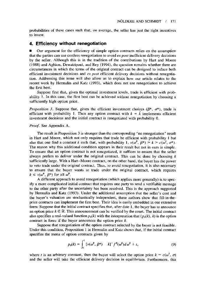
■ Our argument for the efficiency of simple option contracts relies on the assumptionthat the parties can use costless renegotiation to avoid ex post inefficient delivery decisionsby the seller. Although this is in the tradition of the contributions by Hart and Moore(1988) and Aghion, Dewatripont, and Rey (1994), the question remains whether there arecircumstances in which the terms of the original contract can be designed to induce bothefficient investment decisions and ex post efficient delive~ decisions without renegotia-tion. Addressing this issue will also allow us to explain how our article relates to therecent work by Hermalin and Katz (1993), which does not use renegotiation to achievethe first best.
Suppose first that, given the optimal investment levels, trade is efficient with prob-ability 1. In this case, the first best can be achieved without renegotiation by choosing asufficiently high option price.
Proposition 3. Suppose that, given the efficient investment choices (’*, d), trade isefficient with probability 1. Then any option contract with k = ~ implements efficientinvestment decisions and the initial contract is renegotiated with probability O.
Proof. See Appendix A.
The result in Proposition 3 is stronger than the corresponding “no renegotiation” resultin Hart and Moore, which not only requires that trade be efficient with probability 1 butalso that one find a constant k such that, with probability 1, V(OB,P*) = k = C(as, a*),
The reason why this additional condition appears in their result but not in ours is simple.To ensure that an option contract is not renegotiated, it suffices to ensure that the selleralways prefers to deliver under the original contract. This can be done by choosing k
sufficiently large. With a Hart-Moore contract, on the other hand, the buyer has the powerto veto trade under the original contract. Thus, to avoid renegotiation, it is also necessaryto ensure that the buyer wants to trade under the original contract, which requiresk s V(OJB,/3*) for all tiB.
A different approach to avoid renegotiation (which applies more generally) is to spec-ify a more complicated initial contract that requires one party to send a verifiable messageto the other party after the uncertainty has been resolved. This is the approach suggestedby Hermalin and Katz (1993). Under the additional assumption that the seller’s cost andthe buyer’s valuation are stochastically independent, these authors show that fill-in-the-price contracts can implement the first best. Their idea is easily embedded in our extensiveform: Suppose that the initial contract specifies that, after date 1, the buyer has to announcean option price k E k!. This announcement can be verified by the court. The initial contractalso specifies a real-valued function po(k) with the interpretation that (pO(k), k) is the optioncontract in force if the buyer announces the option price k.
Suppose that renegotiation of the option contract selected by the buyer is not feasible.Under this condition, Proposition 1 in Hermalin and Katz shows that, if the initial contractspecifies the menu of option contracts given by
Jpo(k) = ‘ [V(f.f, /3’) – k]+ f ‘(ti’)da? + t,o
(9)
where t is an arbitrary constant, then the buyer will select the option price k = C(OJS,u)
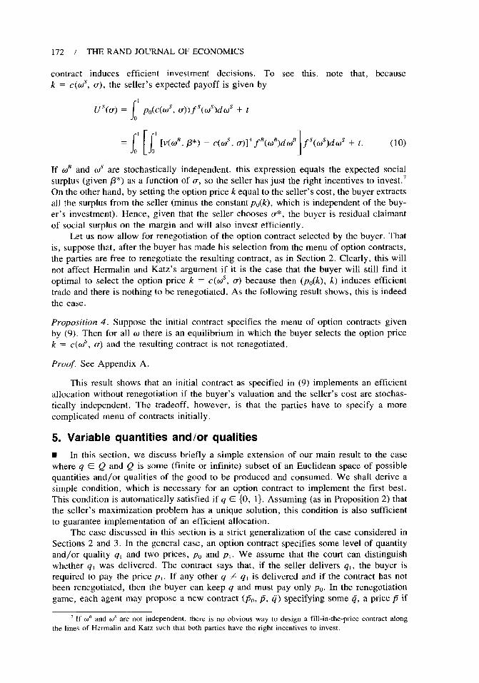
and the seller will take the efficient delivery decision in equilibrium. Furthermore, this
172 / THE RAND JOURNAL OF ECONOMICS
contract induces efficient investment decisions. To see this, note that, becausek = C(ws, U), the seller’s expected payoff is given by
/
1
us(a) = Po(dos, d) fs((os)d(ds + to
I .1—— J[J 1
[v(toB, p“) – C(J, cr)]+f”((d’)dk)’fs((lf)da)’ + f. (10)00
If o’ and @s are stochastically independent, this expression equals the expected socialsurplus (given /3*) as a function of cr, so the seller has just the right incentives to invest.’On the other hand, by setting the option price k equal to the seller’s cost, the buyer extractsall the surplus from the seller (minus the constant po(k), which is independent of the buy-er’s investment). Hence, given that the seller chooses W*, the buyer is residual claimantof social surplus on the margin and will also invest efficiently.
Let us now allow for renegotiation of the option contract selected by the buyer. Thatis, suppose that, after the buyer has made his selection from the menu of option contracts,the parties are free to renegotiate the resulting contract, as in Section 2. Clearly, this willnot affect Hermalin and Katz’s argument if it is the case that the buyer will still find itoptimal to select the option price k = C(us, @ because then (pO(k), k) induces efficienttrade and there is nothing to be renegotiated. As the following result shows, this is indeedthe case.
Proposition 4. Suppose the initial contract specifies the menu of option contracts givenby (9). Then for all o there is an equilibrium in which the buyer selects the option pricek = C(cos, cr) and the resulting contract is not renegotiated.
Proof. See Appendix A.
This result shows that an initial contract as specified in (9) implements an efficientallocation without renegotiation if the buyer’s valuation and the seller’s cost are stochas-tically independent. The tradeoff, however, is that the parties have to specify a morecomplicated menu of contracts initially.
5. Variable quantities and/or qualities
9 In this section, we discuss briefly a simple extension of our main result to the casewhere q E Q and Q is some (finite or infinite) subset of an Euclidean space of possiblequantities and/or qualities of the good to be produced and consumed. We shall derive asimple condition, which is necessary for an option contract to implement the first best.This condition is automatically satisfied if q ~ {O, 1}. Assuming (as in Proposition 2) thatthe seller’s maximization problem has a unique solution, this condition is also sufficientto guarantee implementation of an efficient allocation.
The case discussed in this section is a strict generalization of the case considered inSections 2 and 3. In the general case, an option contract specifies some level of quantityand/or quality qi and two prices, PO and p,. We assume that the court can distinguishwhether q, was delivered. The contract says that, if the seller delivers ql, the buyer isrequired to pay the price p,. If any other q # q} is delivered and if the contract has notbeen renegotiated, then the buyer can keep q and must pay only pO. In the renegotiationgame, each agent may propose a new contract (j%, P, @ specifying some ~, a price P if
‘ It’ U“ and w’ are nut inde~nden[, there is no obvious way to design a fill-in-the-price contract alongthe lines of Hermal in and Katz such that both parties have the right incentives to invest.

NOLDEKE
@is delivered, and a no-trade payment j%.8 The utilities of thegiven by
uB=v(q, oB, @ – p–h~(p)
u‘= p–c(q, ti~,a)-h~(a).
AND SCHMIDT / 173
buyer and the seller are
(11)
(12)
Trade of q takes place if and only if the seller delivers q at date 2 and the buyer acceptsdelivery. Let qO E Q denote the event of no trade with v(qa, “) = c(qO, “) = O. For allq # qO, the valuation of the buyer and the production cost of the seller are strictly positive.As before, we also assume that production costs are nonincreasing in @ and continuous.The first-best investment levels maximize
11W(p, @ =
JJ[ 1max {v(q, aB, /3) – c(q, J, a)} f(o)dri?citos – If(p) – F(u).00 qeQ
(13)
Assume that there exists a unique pair (/3*, d) maximizing this expression, and let
Q*(@, P, d = wma%d(q,~”> P) – dq, o’, d} be nonerwty. The following Prop-osition summarizes the outcome of the renegotiation game and is the counterpart of Prop-osition 1:
Proposition 5. Let (PO, p,, gl) be the initial option contract signed at date O. Given in-vestment levels ~ E [0, ~] and u ~ [0, &], the specifications of trade satisfiesq c Q*(w, ~, m) and the payment from the buyer to the seller is given by
(i) if p, – pO s c(q,, @s, u), then p = p~ + C(q, rils, a)
(ii) if pl – p. > c(ql, Ws, m), then P = PI + C(9! as, @ – C(q,, J, a).
The formal proof is omitted because it is a simple generalization of the proof ofProposition 1. To give some intuition for it, consider two cases in turn.
(i) If PI – p. < c(q,, O, u), then in the absence of renegotiation, the seller will refuseto trade (q = go). Clearly, delivering q, is not profitable. Furthermore, it is neverprofitable for the seller to deliver any other ~ # q, because production costs are pos-itive, whereas the payment p. is independent of whether he delivers ~ or refuses totrade. If go E Q*(o, ~, u), i.e., no trade is efficient, then there is no scope forrenegotiation and the outcome is given by (go, PO). So suppose that go @ Q*. Theseller is only willing to deliver ~ # go if he gets a renegotiation offer signed by thebuyer saying that ~ will be traded for payment ~, where @ has to be large enough togive the seller at least the utility of his default point (go, po). Hence, the buyer’srenegotiation offer will satisfy
p – C(4, (Os, u) = p~ (14)
and the seller will accept this contract, deliver ~, and enforce p. Because the buyer
* Although an option contract unambiguously specifies what payments should be enforced by the courts,it could be argued that such a contract is unlikeI y to be enforceable in practice. In particular, if the sellerchooses a specification q that departs only slightly from the q, agreed upon in the contract, the price dropsfrom p, to POeven if the utility loss incurred by the buyer is small. However, when the courts feel that damagepayments depart too much from actual (or expected) damages, they may dismiss them as inadequate or punitiveand refuse to enforce them. See Edlin and Reichelstein (1993) and the literature cited there. This problem iscommon to most theoretical analyses of contracts. Note, however, that the general logic of our arguments
aPPhe5 even If the courts enfOrCe P, for any 9 delivered by the seller, which is in a neighborhood of q,, aslong as this implicit option contract induces overinvestment. We arc grateful to Mike Riordan for this obserwticrn.

174 / THE RAND JOURNAL OF ECONOMICS
can extract all the surplus from the seller, the optimal renegotiation offer satisfiesg E Q*(ti, /3, m).
(ii) If PI – PO > C(qi, ~, u), the default point of the seller is to deliver ql. If q, isthe efficient level of trade, there is nothing to renegotiate, so suppose that
q] @ Q*(w> A d. Again, the buyer h= to make an offer that induces the seller notto deliver ql. Thus, in equilibrium, the buyer will offer (~, P) such that
p C(1, 0s, u) = p, – C(q,, J, a) (15)
and ~ C Q*(o, ~, u). Again, the seller will accept this offer, deliver ~, and enforce
P.
Anticipating this renegotiation outcome, the expected utilities of the agents are given by
JI
— F(D) – pa – [k – C(q, , al”, U)]+fs(cos)dos (16)o
/
I
US(U,~, pa, k, q,) = –F(v) + p(j + [k – C(q, , J, U)]+”fs(tis)do’. (17)o
For any option contract, the buyer’s expected payoff coincides with social welfareminus a term that is independent of his investment decision. Thus, the buyer will alwaysinvest efficiently. The investment incentives of the seller depend on the choice of q I andk, and we let Xqj, k) denote the set of maximizers of ( 17) given these parameters. Also,let k(ql ) = maxti~,v c(q,, J, 0).
The crucial consideration in determining whether it is possible to achieve the firstbest with an option contract is whether it is possible to induce the seller to invest at leastthe efficient amount by specifying a sufficiently high option price. In Lemma 2, we givea necessary and sufficient condition for this to be the case. The condition requires thatthere exists a YI such that the seller is induced to overinvest if hc receives the returns forhis investment with probability 1. Note that, if Q = {O, 1}, this condition is always sat-isfied, as was shown by Lemma 1.
Lemma 2. There exists an option contract that induces the seller to invest at least theefficient amount, i.e., 3(ql, k): a* s maxZ(q,, k), if and only if there exists q, E Q suchthat
30 = d: cr E argmaxs
– C(q, , J, cr’)fs(aljdos – hs(o”). (18)u’ o
In particular, the first best cannot be implemented if (18) fails for all q].
Proof. See Appendix A.
The economic interpretation of (18) will be discussed after Proposition 6, which isthe counterpart to Proposition 2 .Y
‘ As in Proposition 2, the following result imposes a uniqueness requirement on the solution to the seller’smaximization problem. Note that this assumption is only required for one particular choice of q,. Specifically,it suffices to find a specification q, such that ( 18) holds and such that C(ql, ~, .) satisfies the conditions discussedin Appendix B.

NOLDEKE AND SCHMIDT / 175
Proposition 6. Suppose there exists a q, satisfying (18). Furthermore, assume that, giventhis q,, there exists a unique ~k) maximizing the seller’s payoff function (17) for allk c [0, ~(ql)]. Then there exists an option contract (PO, PI, q,) that implements efficientinvestment and trade decisions. Furthermore, any division of the ex ante surplus can beachieved by choosing PO appropriately.
Proof. Let q, be as specified in the statement of the proposition. Then 0-(0) = O (cf. theproof of Lemma 1) and a(~(ql)) ~ m“ (cf. Lemma 2). The result then follows from theuniqueness assumption on a(k) as in the proof of Proposition 2. Q.E.D.
In the literature on incomplete contracts, it has often been claimed that q is noncon-tractible ex ante because it is too difficult to specify the good in advance, in particularbecause the optimal specification may depend on a complex realization of the state of theworld. The above proposition shows that optimal investment incentives can be given witha simple option contract in which only one specification of the good (q,) has to be de-scribed.’0 If this good were traded with probability 1, the seller would be induced tooverinvest. By choosing the option price k appropriately, the incentives to overinvest (ifq, is the default point) and to underinvest (if go is the default point) can be balanced suchthat the seller will invest efficiently, whereas renegotiation ensures efficient trade.
However, a necessary condition for an option contract to implement the first best isthat (18) holds. If q is interpreted as the quantity to be produced, this condition is innoc-uous. It is natural to assume that the marginal benefit of investment is nondecreasing withthe quantity of trade in all states of the world. Thus, it would be sufficient to pick q[ asthe largest q that is traded with positive probability in the first best in order to induce theseller to overinvest. If q represents different levels of quality, which can be ordered alongthe real line such that higher levels of quality make a higher level of investment moredesirable in all states of the world, (18) is also unproblematic. However, if q stands fordifferent specifications of the good and, if for any specification, the productivity of theinvestment depends on the realization of the state of the world, then there are naturalexamples in which (18) is violated. As an ilhtstration, suppose that, for any given q] ~ Q,
the investment pays off only for some states of the world but is unproductive in others.Thus, if any fixed q, is traded with probability 1, only some modest investment is optimal.On the other hand, the ex post efficient q* depends on the state of the world. Thus, giventhat q*(~) will be traded, the investment may now pay off in all states of the world. Hence,the socially optimal investment level @ may be higher than the optimal investment levelgiven any fixed q, E Q.
A related problem that may prevent the implementation of the first best with a simpleoption contract is the possibility that investments may be multidimensional. For example,suppose that the seller has a choice between investing in a general purpose technology orin one of several specific purpose technologies that are only useful if a given specificationis produced. Because there is uncertainty about the optimal specification ex ante, it maybe efficient to invest in the general purpose technology, whereas an option contract willprovide the seller with a strong incentive to invest in a technology that is tailored to thespecification in the option contract. Although the analysis of the hold-up problem withmultidimensional investment decisions is beyond the scope of this article, it clearly is animportant topic for future research.
‘0Note that the incomplete contracts literature typically assumes that it is possible to contractually describea single specification ex post, so h should also be possible to do this ex ume. However, it is essential that this
specification be descri~d unambiguously, which may be more difficult if the good does not yet exist (e g., ifsome research is necessary to deveIop it).

176 / THE RAND JOURNAL OF ECONOMICS
6. Conclusions
■ We have shown that, in the canonical hold-up model introduced by Hart and Moore(1988), the first best can be achieved if the courts can verify delivery of the good by theseller. This can be done using a very simple contract that does not rely on renegotiationdesign or complicated revelation mechanisms. The crucial feature of the contracts we usedis that one of the parties can decide unilaterally whether trade takes place. This is whywe called them option contracts.
Throughout the article, we restricted attention to the case in which both parties arerisk neutml and in which there are only indirect externalities of the investment decisions. 11This is the case considered in most of the hold-up and incomplete contracts literature. Wequestion whether an option contract can implement the first best in more complex envi-ronments in which these assumptions are relaxed. There is no hope that an option contmctcan allocate risk efficiently. This would require that the default point of renegotiation varycontinuously with the realization of the state of the world, which is impossible to achievewith the very simple instrument considered in this article.’2 Option contracts are moresuccessful in dealing with one-sided direct externalities. Suppose that the investment ofthe seller affects the valuation of the buyer directly, e.g., because it has an impact on thequality of the good. In this case, an option contract can induce both parties to investefficiently, provided that it is still possible to induce the seller to overinvest. In this case,we can choose the option price such that, in expectation, the seller has just the rightincentives to invest. Given that he chooses the first-best level m*, the unique best responseof the buyer is to also invest efficiently. On the other hand, if there is a two-sided directexternality, option contracts fail to implement the first best. Although the seller can begiven the right incentives as just described, the buyer will not take into account the impactof his investment on the costs of the seller. 13An interesting question for future researchis whether there are other contracts that give optimal investment incentives in this caseand, in particular, whether the first best can be achieved using simple real-world contracts,which do not rely on complex revelation mechanisms.
Appendix A
■ proofs of Propositions 1, 3, and 4 and proofs of Lemmas 1 and 2 follow.
Proof of Proposition 1. We first show that the seller does not make a renegotiation offer in equilibrium. Givenour assumption that an agent makes a renegotiation offer only if it strictly increases his payoff, it suffices toshow that the seller has nothing to lose from dropping any renegotiation offer he might make. To see this,crrnsicter a subgame starting after renegotiation offers (pi. p’,), i 6 {B, S}, have been made14 and let
PY = max{pd, JJS}. we argue that the seller’s continuation payoff cannot exceed max.{p~ – de}. Suppose theseller chooses d = 0. The buyer can ensure that his payment does not exceed PT by withholding any contractthe seller may have sent. Hence. the seller’s expected continuation payoff (after he has chosen d = O), whichis uniquely determined because the contract submission game is zero sum, must be smaller than p}. If thesel Ier chooses d = 1, an equivalent argument implies that the seller’s expected continuation payoff cannotexceed p~ — ~. we should note that the seller can ensure the payoff max,,{p7 – dc} by nut making a rene-
gotiation offer, choosing the appropriate delivery decision, and submitting the contract that specifies the pricep~ to the court. Because the buyer has only the initial contract to submit, the payment pJ will then be enforcedby the court.
Consider now a subgame that results after the buyer (or no agent) has made a renegotiation offer. In asuhgame-perfect equilibrium, the seller must choose d to maximize max{p; , p~] – d. c and then submit the
‘‘ The externalities are indirect because (3(u) does not affect the cost of the seller (valuation of the buyer)directly but affects his utility only indirectly through the probability of trade.
“ Aghion, Dewatripont, and Rey (1994) show that this can be achieved using a complex revelationmechanism.
“ This can be seen from the buyer’s utility function (4) given in Crmrllary 1. If ~ affects c, the last termof this expression is no longer a constant.
“ To simP]ifY notation, we let (F:,, p’,) = (po, p)) if player i did not make a renegotiatlon Offer.

NOLDEKE AND SCHMIDT / 177
most profitable contract to the coufi. If the buyer does not make a renegotiation offer, the seller will thuschoose not to deliver if strict inequality holds in case (i) and will choose to deliver in case (ii). For each ofthese cases, two subcases have to be distinguished:
(is) p, – p, < c(ro’, a) and v(af, B) s C(OJS,U). In this case, g = Ois an efficient outcome, and the sellerdoes not want to trade given the initial prices. It is easy to see that there does not exist a renegotiationoffer the buyer could make that would increase his payoff. Hence, the buyer does not make a renegotiationoffer. In any subgame-perfect equilibrium, the seller will thus not deliver, implying q = O and a transferpayment p = pO.
(ib) PI – PO < C(OS, d and V(WB,~) > C(OJS,u). In this case, trade would be efficient, but if the buyer does
(iia)
not make a renegotiation offer, the seller is not going to trade because not delivering gives himp. > p, – c. Because the selIer’s delivery decision depends only on the difference between the trade and
the no-trade price, the buyer will not offer to raise the no-trade price in a subgame-perfect equilibrium.The buyer could send a renegotiation offer to the seller, raising the trade payment to p: = p. + c + cand leaving the no-trade price unchanged. For all 6>0, the seller will respond by delivering and enforcingthe payment ~!. If the seller also responds by delivering for c = O, then it is optimal for the buyer tooffer a new contract with P; = PO + C(tis, U). Indeed, no best response would exist for the buyer if theseller were not to deliver given this offer. Thus, it follows that, in a subgame-perfect equilibrium, thebuyer offers a new contract with Ff’ = p. + c(J. u) and the seller chooses to deliver and then enforcesthe transfer J7Y. Note that, because v > 0, every best response of the buyer specifies that he acceptsdelivery. Hence, q = 1.
PI – Po > c(~s, @ ~d v(~’, @ < c(@’, u). NO trade would be efficient, but if the buyer does not makea renegotiation offer, the seller will choose to deliver. As in case (ib), the buyer can strictly increase hisutility by making a renegotiation offer, in this case, one that raises the no-trade payment top% = p, – c + E. For all E > 0, the seller will respond to such an offer by not delivering, implying~ = 0, and enforcing the price ~~. Hence, in equilibrium, the buyer will offer ~~ = p, – c and the seller
will not deliver and enforce pg.
(iib) pl – PO > C(ws, a) and V(OB,f3) a C(ws, cr). In this case, the seller wants to deliver given the old pricesand trade is efficient. As in case (is), there is no renegotiation offer the buyer could make that wouldimprove his utiiity. Thus, the seller will deliver and the transfer is pl.
Finally, we need to consider the case p, – PO= C(OJS,m). Then the seller is indifferent whether to deliverunder the terms of the initial contract. If v = c, any decision by the seller results in efficient trade and thebuyer is indifferent between receiving the good and paying p, and not receiving it and paying pO, so that hehas nothing to gain from making a renegotiation offer. If v # c, a best response for the buyer only exists ifthe seller takes the efficient delivery decision, either without receiving a renegotiation offer or after receivinga renegotiation offer that specifies exactly the same prices as the initial contract. Q .E.D.
Proof of Lemma 1. Letk = 0. Because production costs are nonnegative, the seller’s problem is then tomaximize
u~(po, o, u) = p, – hyu). (Al)
Because h’ is increasing in m, the only solution to this problem is u = O. Hence, because U* 20, the firstclaim follows.
Let k = k. Given (PO k), the seller’s problem is to maximize
US(PO,k, u) =[
(k - C(ws, u)) f’(ws)da# + p. – h’(u).
This problem has the same set of maximizers as the problem
11max
11(v(ro’, ~“) - C(SIJ’,u)) f(w)dafdw’ – h’(u) – h8(~*),
.
(A2)
(A3)
which, in turn, is the same as
11max W(~*, CT)–
U[C(OS, u) – v(d, (3*)]+f(to)dwsdaf’. (A4)
.
Because C(OJ’,u) is nonincreming in u for all w’, the integral added to W(P*, cr) is nondecreasing in ~. Hence,
this problem cannot have a maximizer u < U*. Q .E.D.

178 / THE RAND JOURNAL OF ECONOMICS
Proof of Proposition 3. From Lemma 1 ~ e X(k) > u z u“. Consider (A4) in the proof of Lemma 1. Underthe stated condition
11
( I [C,of,a) - v(ti’,m,+f(ti)dti’das” = 0 (A5).!QJO
for all u a U*. Thus, for all rr z u“ the seller’s maximization problem is equivalent to maximizing W(~*, u)plus a constant. Consequently, u“ is the unique optimal investment choice for the seller. Hence, the buyer willalso choose ~ = B*. Q.E.D.
Prooj of Proposition 4. It follows from Proposition 1 that, if the buyer selects an option contract that makesit optimal for the seller to take the efficient delivery decision, then this contract will not be renegotiated andthe seller will indeed trade efficiently. Hence, for all such choices, the buyer’s continuation payoff is as spec-ified in Hermalin and Katz (1993). We must still show that the buyer cannot strictly gain by selecting a contractthat would be renegotiated instead of choosing k = c (w’, a). There are two cases to consider.
First, suppose V(WE,/3) > C(OS, U), that is, trade is efficient. It follows from Proposition 1 that rene-gotiation will occur if and only if the buyer selects k < c(J, u). The resulting option contract (pO(k), k) willbe renegotiated to the contract (p,(k), C(ws, d) and the seller will deliver, so the resulting payment by thebuyer is given by po(k) + C(WS, u). If the buyer chooses k = c(J, m) instead, the resulting option contract
will not be renegotiated, the seller will deliver, and the buyer’s payment is given by PAc(wS, a)) + C(as, ~).Because k < C(O’$,u) implies p“(k) ~ p,,(c(a”, u)), it follows that choosing k < C(tis, u) cannot increase thebuyer’s payoff.
Second, suppose X~H, /3) < c(~s, ~), that is, trade is inefficient. It follows from Proposition 1 thatrenegotiation will occur if and only if the buyer selects an option price k > C(WS, rr). The resulting optioncontract (p”(k), k) will be renegotiated to the contract (pO(k) + k – C(tis, u), C(tis, u)), the seller will notdeliver, and the buyer’s payment is given by p,(k) + k – C(ws, u). If the buyer chooses k = c(~s, u) instead,the resulting option contract will not be renegotiated, the seller will not deliver, and the buyer’s payment isgiven by p,(c(ws, u)). Because k > C-(WS,u) implies po(c(os, u)) – po(k) < k – C(os, u), it follows that the
buyer cannot increase his payoff by choosing k > c(o”’, u). QED.
Proof of Lemma 2. Note that, for all q, ~ Q and k ~ k(q, ),
I(q,, k) = argmax –J’
C(9I , J, U)”fs(us)d@s – h$(a). (A6). 0
Suppose q, satisfies ( 18). Then (A6) implies maxX(q,, k(q, )) > rr*.Suppose q, does not satisfy (1 8). We show that Vk: maxX(q,, k) < u*. Fork z k(ql). this follows from
(A6). Consider k < ~. Then
,-,U“(u, ~, p,, k(q, ).q,) – US(U. ~, p,, k, q,) =
1
[k(q, ) – max{k, c(q,, o’, u)}]’ .fs(wf)d~s
Because production costs are nonincreasing in u, [his expression is nondecreasing in a. It follows that
Vk < k(q,): u G E(q,, k) > u ~ mx~(qi, k(q,)) < u*. Hence, if there is no q, satisfying ( 18), then
V(q,, k): max Xq,, k) < u*. Q.E.D.
Appendix B
■ Conditions on the cost functions h’(.) and c(., .) follow
Assume that c and hs are twice continuously differentiable with &-/da <0, d’c/dc? a O, dc/&os >0,and dhs/du > 0. For every option price k and investment level U, there exists a unique @s(k, m) E [0, 1] suchthat
(i)S> @“(k, u) ~ C(6JS,u) > k,
The seller’s utility function can thus be written as
1
m’$(k.m)f/s(PO, k, o) = [k – C(OS, a)] fs(tis)dtis + p“ - h’(a), (Bl)
Taking the derivative with respect to a, we obtain
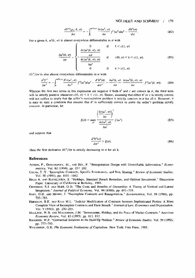
NOLDEKE AND SCHMIDT / 179
N7s(po, k, u)
1
‘s(k’o)ac(ti~, a)
13cr ‘–~ fs(cos)dros – ~,
da(B2)
For a given k, tis(k, u) is almost everywhere differentiable in u with
[
o if k<c(l, cr)
ac(d-(k, (r), u)
Ow’(k, u) dw— . .ac(o’(k, u), a)
if C(o, u)<k<c(l, cr).au
am’o if k>c(l, a)
dUs/da is also almost everywhere differentiable in u with
a’u’
–1
‘S(””JXc(a)’, a) d’hs(w) b’(k, U) ac(ws(k, u), U)— — f’(.’)d.’ - ~ – —aO’ – – drrz au au
~f’(af(k, u)). (B4)
(B3)
Whereas the first two terms in this expression are negative if both h’ and c are convex in a, the third termwill be strictly positive whenever c(O, U) < k < C(1, @. Hence, assuming that either hs or c is strictly convexwill not suffice to imply that the seller’s maximization problem is strictly concave in u for all k. However, itis easy to state a condition that ensures that hs is sufficiently convex to make the seller’s problem strictlyconcave. In particular, let
()
ac(~$, ~) 2
f(u) = y ac(;, ~, f(w’)
au’
and suppose that
d’hs(cr)— > g(u).
do’
(B5)
(B6)
Then the first derivative dUs/da is strictly decreasing in u for all k
References
AGHION,P., DEWATRPONT,M., ANDREY, P. “Renegotiation Design with Unverifiable Information. ” Ecorro-metrica, Vol. 62 (1994), pp. 257–282.
CHUNG,T.-Y. “Incomplete Contracts, Specific Investments, and Risk Sharing. ” Review of Economic Srudies,vol. 58 (1991), pp. 1031-1042.
EDLINA. ANDREICHELSTEIN,S. “Holdups, StandardBreach Remedies,and Optimal Investment.” DiscussionPaper. University of California at Berkeley, 1993.
GROSSMAN,S .J. AND HART, O.D. “The Costs and Benefits of Ownership: A Theory of Vertical and LateralIntegration. ” .Jourrral of Polirical Econc?my, Vol. 94 (1986), pp. 691 –7 19.
HART, O.D. ANDMOORE, J. “Incomplete Contracts and Renegotiation. ” Econmnetrica, Vol. 56 (1988), pp.755–785
HLKMALIN,B .E. ANDKATZ M.L. “Judicial Modification of Contracts between Sophisticated Parties: A MoreComplete View of Incomplete Contracts and Their Breach ~”Journal of Law, Economics and Orgarriza/iorr,Vol. 9 ( 1993), pp. 230-255.
MACLEOD, W. B. ANDMALCOMSON,J .M. “Investments, Holdup, and the Form of Market Contracts. ” American.Ecorromic Review, Vol. 83 (1993), pp. 81 1–837.
RDGERSON,W.P. “Contractual Solutions to the Hold-Up Problem. ” Review of Economic Studies, Vol. 59 (1992),pp. 777–793.
WILLIAMSON,O.E. The Economic Institutions of Capitalism. New York: Free Press, 1985.