Optimum configuration of shell-and-tube heat exchangers for the use inlow-temperature organic Rankine cyclesI

Daniel Walravena,c, Ben Laenenb,c, William D’haeseleera,c,∗

aUniversity of Leuven (KU Leuven) Energy Institute - TME branch (Applied Mechanics and Energy Conversion),Celestijnenlaan 300A box 2421, B-3001 Leuven, Belgium

bFlemish Institute for Technological Research (VITO), Boeretang 200, B-2400 Mol, BelgiumcEnergyVille (joint venture of VITO and KU Leuven), Dennenstraat 7, B-3600 Genk, Belgium

Abstract

In this paper, a first step towards a system optimization of organic Rankine cycles (ORCs) is taken byoptimizing the cycle parameters together with the configuration of shell-and-tube heat exchangers. Inthis way every heat exchanger has the optimum allocation of heat-exchanger surface, pressure drop andpinch-point-temperature difference for the given boundary conditions. Different tube configurations areinvestigated in this paper. It is concluded that the 30◦-tube configurations should be used for the single-phase heat exchangers and the 60◦-tube configuration for the two-phase heat exchangers. The performanceof subcritical cycles can be strongly improved by adding a second pressure level. Recuperated cycles areonly useful when the temperature of the heat source after the ORC should be relatively high.

Keywords: ORC, Shell-and-tube heat exchanger, System optimization

1. Introduction

The amount of energy stored in low-temperature geothermal heat sources is huge [1] but the conversionto electricity is inefficient due to the low temperature. Much research has been performed to maximizethis conversion efficiency by the use of organic Rankine cycles (ORC) [2–5]. Most of these studies optimizethe cycle parameters (pressures, temperatures and mass flow rates) for different working fluids, but makesimplifying assumptions about the components. Heat exchangers are assumed to be ideal or to have a fixedpressure drop, pinch-point temperature differences are assumed to be fixed, etc. The choice of these pa-rameters has an important influence on the performance of the ORC and on the total cost of the installation.

Many authors have already investigated the optimal configuration of shell-and-tube heat exchangers [6–9],plate heat exchangers [10, 11], cooling systems [12–14], etc, but mostly independently of the thermodynamiccycle in which they are supposed to operate. When optimizing components, assumptions have to be madeabout the system in which the components will work (e.g. maximum allowed pressure drop). To avoidnon-optimal assumptions, it is best to optimize the cycle and the components together and to perform a fullsystem optimization. In this way, all components are adjusted to each other and to the cycle.

This issue is already touched upon in the literature. The influence of heat exchangers on the cycle wasinvestigated by Madhawa Hettiarachchi et al. [15]. They minimized the ratio of the total heat-exchangersurface and the net electrical power produced by the cycle. The configuration of the heat exchangers was

IPublished version: http://dx.doi.org/10.1016/j.enconman.2014.03.066∗Corresponding author. Tel.: +32 16 32 25 11; fax: +32 16 32 29 85.Email addresses: Daniel.Walraven@mech.kuleuven.be (Daniel Walraven), Ben.Laenen@vito.be (Ben Laenen),

William.Dhaeseleer@mech.kuleuven.be (William D’haeseleer)

Preprint submitted to Energy Conversion and Management March 26, 2014

fixed. Franco and Villani [16] divided the ORC in two levels: the system level and the component level.First, the authors optimized the system level. In a next step, they used this optimum system configurationto find the optimal configuration of the components. An iteration between both levels was needed to cometo the final solution. The optimal system configuration obtained this way will probably be very close to theone in the first iteration.

In this paper, a first step towards a system optimization of an ORC is taken by including shell-and-tube heatexchangers in the optimization. The shell-and-tube heat exchangers are modeled with the Bell-Delawaremethod [17, 18], which is a mature model and can be used for single-phase flow, condensing and evaporation.The shell-and-tube heat-exchanger model is added to a previously developed ORC model [4] in which theheat exchangers were assumed to be ideal.

2. Organic Rankine cycle

In this paper, different types of organic Rankine cycles are simulated. They can be of the simple or recu-perated type, be subcritical or transcritical and can have one or two pressure levels. Figure 1a shows thescheme of a single-pressure, recuperated ORC. The liquid working fluid is first pumped to a high pressure(1→2), heated by the heat source in the recuperator (2→3), in the economizer (3→4), in the evaporator(4→5) and in the superheater (5→6). Then the working fluid is expanded in the turbine (6→7), cooled inthe recuperator (7→8), in the desuperheater (8→9) and in the condenser (9→1). Not all heat exchangers arenecessary in all circumstances. Dry fluids, wet fluids and transcritical fluids often do not need a superheater,desuperheater or evaporator, respectively. A simple ORC is obtained by omitting the recuperator in figure1a.

Cooling outCooling in

Heat source inHeat source out

1

2

3

4 56

7

8

9

(a) Single-pressure

Cooling outCooling in

Heat source in

Hea

tso

urc

eou

t

1 9 7

2 4b 5b 6b

1a2a 4a 5a 6a

(b) Double-pressure

Figure 1: Scheme of a single-pressure, recuperated (a) and double-pressure, simple (b) ORC.

Figure 1b shows the scheme of a double-pressure, simple ORC. The liquid working fluid is first pumpedto an intermediate pressure (1→2) and heated in the intermediate pressure economizer (2→1a/4b). A partof the working fluid remains at the intermediate pressure and is heated in the intermediate pressure evap-orator (4b →5b) and superheater (5b →6b). The other part is pumped to a high pressure (1a →2a), heatedin the high pressure economizer (2a →4a), evaporator (4a →5a) and superheater (5a →6a). Both state 6a

and 6b are expanded in the turbine (6a/6b →7) and afterward cooled in the desuperheater (7→9) and inthe condenser (9→1). In the case of a double-pressure, recuperated ORC, a recuperator is used which coolsdown state 7 and heats up state 2, analogous to the single-pressure case.

2

In all configurations it is assumed that state 1 is saturated liquid and that the isentropic efficiencies ofthe pump and turbine are 80 and 85%, respectively. More information on the ORC model can be found inWalraven et al. [4], on which this work is based. Instead of assuming a fixed pinch-point temperature differ-ence and ideal heat exchangers, models are used to calculate the heat transfer coefficients and pressure dropsin each heat exchanger. These models are described in the following sections. The cycle and componentsare optimized together in order to maximize the electricity production from a given heat source.

3. Shell-and-tube heat exchanger

3.1. Geometry

Shell-and-tube heat exchangers can be constructed with many different configurations. In this paper it ischosen to only investigate the TEMA E type. This is the most basic type, with a single shell pass and withthe inlet and the outlet at the opposite ends of the shell. The working fluid always flows on the shellside, somodels for the pressure drop and heat transfer coefficient in single-phase flow, evaporation and condensationin a TEMA E shell are needed. The tube-side fluid (the heat source and heat sink) will always be singlephase.

Lb,cLb,i

Lb,o

Ds

lc

pt

Dotl

θb

θctl

do

Dctl

Window

Cro

ss-

flowIn

let

Ou

tlet

Figure 2: Shell-and-tube geometrical characteristics. Figure adapted from Shah and Sekulic [18].

Figure 2 shows the basic geometrical characteristics of a shell-and-tube heat exchanger. These are theshell outside diameter Ds, the outside diameter of a tube do, the pitch between the tubes pt, the baffle cutlength lc and the baffle spacing at the inlet Lb,i, outlet Lb,o and the center Lb,c. The expressions to calculateother geometrical characteristics are given in Appendix A, which can also be found in the literature [17, 18].The inlet, the outlet, a crossflow and a window section are also indicated on figure 2.

3.2. Bell-Delaware

The Bell-Delaware method [17, 18], which is based on the reasoning of Tinker [19], is used to calculate thepressure drop and heat-transfer coefficient on the shellside. Tinker [19] divided the flow in the shell in anumber of streams, as shown in figure 3:

• Stream B: ideal crossflow stream

• Stream A: tube-to-baffle hole leakage stream

• Stream C: bundle-to-shell bypass stream

• Stream E: shell-to-baffle leakage stream

3

Figure 3: Shell-side flow distribution and different streams. Figure from Shah and Sekulic [18].

• Stream F: tube-pass bypass stream

The shell-side heat-transfer coefficient is given as:

hs = hidJcJlJbJsJr, (1)

with hid the ideal heat-transfer coefficient for cross flow over a tube bundle and Jx correction factors fornon-idealities:

• Jc: correction factor for baffle configuration, given by Jc = 0.55 + 0.72Fc

• Jl: correction factor for baffle leakage, given by Jl = 0.44(1 − rs) + [1 − 0.44(1 − rs)]e−2.2rlm with

rs =Ao,sb

Ao,sb+Ao,tband rlm =

Ao,sb+Ao,tb

Ao,cr

• Jb: correction factor for bundle and pass partition bypass. In this paper it is assumed that enoughsealing strips are available, so that Jb = 1.

• Js: correction factor for larger baffle spacing at the inlet and outlet. In this paper it is assumed thatLb,i = Lb,o = Lb,c, so that Js = 1.

• Jr: correction factor for an adverse temperature gradient in laminar flow. This effect is neglected inthis paper because it normally does not occur in optimized heat exchangers and to avoid numericalissues.

The shell-side frictional pressure drop is given as:

[∆ps]fr = [∆pcr]fr + [∆pw]fr + [∆pi−o]fr, (2)

= {(Nb − 1)[∆pb,id]frζb +Nb[∆pw,id]fr} ζl + 2[∆pb,id]fr

(1 +

Nr,cwNr,cc

)ζbζs, (3)

where [∆pcr]fr, [∆pw]fr and [∆pi−o]fr are the frictional pressure drops in the crossflow, window and inlet-outlet sections, respectively. [∆pb,id]fr and [∆pw,id]fr are the ideal frictional pressure drops in crossflow andwindow flow, respectively. Nb is the number of baffles, Nr,cw and Nr,cc the effective number of rows crossedin one window flow and one cross flow, respectively. ζx is a correction factor for non-idealities:

• ζl: correction factor for baffle leakage, given by ζl = exp [−1.33(1 + rs)rplm] with p = [−0.15(1 + rs) + 0.8]

• ζb: correction factor for bypass flow. In this paper it is assumed that enough sealing strips are used,so that ζb = 1.

• ζs: correction factor for larger baffle spacing at the inlet and outlet. In this paper, all baffle spacingsare assumed to be equal, so that ζs = 1.

4

3.3. Ideal heat transfer and pressure drop

To apply the Bell-Delaware method, the ideal heat-transfer coefficient and the ideal pressure drops in thecross flow and window flow section are needed. Correlations for these parameters are given in Appendix Bfor single-phase flow, condensation and evaporation in the shell, together with correlations for single-phaseflow on the tube side, which can also be found in the literature [17, 18].

3.4. Implementation of the models

To account for non-uniform fluid properties, each heat exchanger is divided into five parts with an equal heatload1. This number is chosen because it leads to a reasonable accuracy and calculation time. For each heatexchanger, the configuration (Ds, do, pt, lc and Lb,c), the inlet states at one side of the heat exchanger anda necessary outlet condition (e.g. the working fluid has to be saturated vapor at the end of the evaporator)are needed. With these data, the total heat that has to be transferred in the case of no pressure drop canbe calculated. In each of the five parts one fifth of the total heat will be exchanged. With the equationsabove, the heat-transfer coefficient and the pressure drop in the first part can be calculated. In this way,the state after the first part, the necessary heat-transfer surface and the fictive tube length of the first partL1 can be calculated. This procedure is repeated for the other parts, except in the last part for which theheat to be transferred is corrected for the pressure drop in the previous parts.

The problem which occurs in this procedure is that the frictional pressure drop in the cross-flow sectionis different from the one in the window section, while the heat-transfer coefficient is an average of bothsections. Therefore it is chosen to average the frictional pressure drop in each section:

[∆pparts 1,5s ]fr =

{LiLb,c

[∆pb,id]frζb +

(LiLb,c

− 1

5

)[∆pw,id]fr

}ζl + [∆pb,id]fr

Nr,cwNr,cc

ζbζs, (4)

[∆pparts 2,3,4s ]fr =

{LiLb,c

[∆pb,id]frζb +

(LiLb,c

− 1

5

)[∆pw,id]fr

}ζl, (5)

with Li the fictive length of ith part. Addition of these pressure drops for the different parts, leads again toequation (3) when taking into account that Nb =

∑i Li/Lb,c − 1.

4. Optimization

4.1. Objective function

The goal of the optimization is to find a system configuration which maximizes the mechanical work outputfor a given heat source. This is the same as maximizing the exergetic plant efficiency [4], defined as:

ηplantex =Wnet

msourceesourcein

(6)

with Wnet the net mechanical-power production of the power plant, msource the mass flow of the source andesourcein the flow exergy of the source.

1These parts generally do not have the same physical size.

5

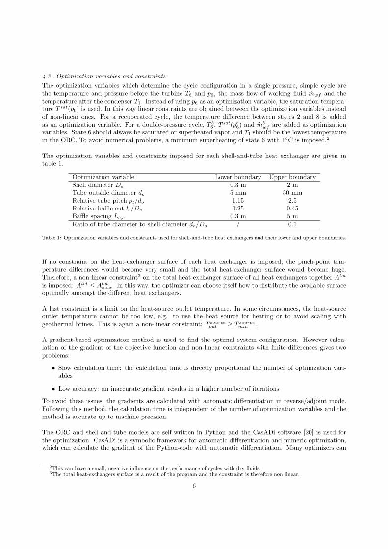
4.2. Optimization variables and constraints

The optimization variables which determine the cycle configuration in a single-pressure, simple cycle arethe temperature and pressure before the turbine T6 and p6, the mass flow of working fluid mwf and thetemperature after the condenser T1. Instead of using p6 as an optimization variable, the saturation tempera-ture T sat(p6) is used. In this way linear constraints are obtained between the optimization variables insteadof non-linear ones. For a recuperated cycle, the temperature difference between states 2 and 8 is addedas an optimization variable. For a double-pressure cycle, T b6 , T sat(pb6) and mb

wf are added as optimizationvariables. State 6 should always be saturated or superheated vapor and T1 should be the lowest temperaturein the ORC. To avoid numerical problems, a minimum superheating of state 6 with 1◦C is imposed.2

The optimization variables and constraints imposed for each shell-and-tube heat exchanger are given intable 1.

Optimization variable Lower boundary Upper boundaryShell diameter Ds 0.3 m 2 mTube outside diameter do 5 mm 50 mmRelative tube pitch pt/do 1.15 2.5Relative baffle cut lc/Ds 0.25 0.45Baffle spacing Lb,c 0.3 m 5 mRatio of tube diameter to shell diameter do/Ds / 0.1

Table 1: Optimization variables and constraints used for shell-and-tube heat exchangers and their lower and upper boundaries.

If no constraint on the heat-exchanger surface of each heat exchanger is imposed, the pinch-point tem-perature differences would become very small and the total heat-exchanger surface would become huge.Therefore, a non-linear constraint3 on the total heat-exchanger surface of all heat exchangers together Atot

is imposed: Atot ≤ Atotmax. In this way, the optimizer can choose itself how to distribute the available surfaceoptimally amongst the different heat exchangers.

A last constraint is a limit on the heat-source outlet temperature. In some circumstances, the heat-sourceoutlet temperature cannot be too low, e.g. to use the heat source for heating or to avoid scaling withgeothermal brines. This is again a non-linear constraint: T sourceout ≥ T sourcemin .

A gradient-based optimization method is used to find the optimal system configuration. However calcu-lation of the gradient of the objective function and non-linear constraints with finite-differences gives twoproblems:

• Slow calculation time: the calculation time is directly proportional the number of optimization vari-ables

• Low accuracy: an inaccurate gradient results in a higher number of iterations

To avoid these issues, the gradients are calculated with automatic differentiation in reverse/adjoint mode.Following this method, the calculation time is independent of the number of optimization variables and themethod is accurate up to machine precision.

The ORC and shell-and-tube models are self-written in Python and the CasADi software [20] is used forthe optimization. CasADi is a symbolic framework for automatic differentiation and numeric optimization,which can calculate the gradient of the Python-code with automatic differentiation. Many optimizers can

2This can have a small, negative influence on the performance of cycles with dry fluids.3The total heat-exchangers surface is a result of the program and the constraint is therefore non linear.

6

be connected to CasADi, but the one used in this paper is WORHP [21].

The fluid properties are obtained from REFPROP [22]. CasADi also needs the derivative of the fluidproperties to calculate the gradient of the objective function and constraints. Therefore the REFPROPfortran code is adapted; the complex-step derivative method [23] is used to obtain the derivative of the fluidproperties. The connection between fortran and Python is made by F2PY [24]. A flow chart which showsthe connection between the different software packages is shown in figure 4.'

&$%

Fluid properties

from RefProp:

Fortran

'&

$%

Fluid properties

derivative:

Fortran

?

Complex-

step

-F2PY

-F2PY

'&

$%

Fluid properties:

Python

'&

$%

Fluid properties

derivative:

Python

-

Value

properties

-

Value

derivative

properties

'&

$%

ORC model:

Python

'&

$%

CasADi

WORHP

?

Value objective

and constraints

-Iteration

Solution

Figure 4: Flow chart showing the connection between the different software packages.

4.3. Advantage system optimization

Instead of a system optimization, it would also be possible to perform an iteration between the optimizationof the system level and the component level as performed by Franco and Villani [16]. First the systemlevel is optimized, while making a guess for the optimal value of the pressure drop and the pinch-point-temperature differences. Afterward the heat exchanger surface of each exchanger is minimized separately,while respecting the load of each heat exchanger. This results in new values of the pressure drop, so that aniteration between the system level and the component level is necessary. The results of this method are thepower output and the heat exchanger surface of each heat exchanger for the given pinch-point-temperaturedifferences. It is possible that a cycle with other values of the pinch-point-temperature differences producesmore electricity for the same total heat exchanger surface and the obtained result is therefore not necessarilya global optimum. So, it is necessary to vary the value of these pinch-point-temperature differences to obtainthe optimal system, which results in large calculation times.

The advantage of the system optimization described in this paper is that the optimal pinch-point-temperaturedifferences are a result of the method, because all components are coupled directly and the optimizationsolver can choose how to allocate the total heat exchanger surface.

5. Results

5.1. Reference parameters

100 kg/s of water is used as the heat source. The parameters for the reference case are given in table 2.The values of these parameters have of course a strong influence on the performance and cost of the powerplant. The main goal of this paper is to show that a system optimization of an ORC can work and theimpact of the reference parameters will be investigated in future work.

5.2. Unconstrained heat source outlet temperature

In this section no limit is imposed on the heat-source outlet temperature. The optimizer can choose theoptimal heat-source outlet temperature to maximize the plant efficiency, while respecting the boundaryconditions.

7

Parameter Symbol ValueHeat source inlet temperature T sourcein 125◦CMaximum allowed heat exchanger surface Atotmax 4000 m2

Cooling fluid inlet temperature T coolingin 20◦CCooling fluid mass flow mcooling 800 kg/s

Table 2: Reference parameters.

5.2.1. Tube configuration shell-and-tube heat exchangers

In this section the influence of the tube configuration (30, 45, 60 or 90◦ - See Appendix A for the layoutof the tubes) on the performance of an ORC is investigated. Figure 5 shows this influence on the exergeticplant efficiency, the net power output and energetic cycle efficiency for single-pressure, simple ORCs. Thiscycle efficiency is defined as:

ηcycleen =Wnet

Q(7)

with Q the heat added to the cycle. Five different cases are shown; the first four cases (30, 45, 60 or 90◦)

Isob

utane

Propan

e

R134a

R218

R227ea

R245fa

R1234yf

RC318

25

30

35

40

45

2

2.5

3

ηplant

ex

[%]

Electricalpow

er[M

W]

30◦ 45◦ 60◦ 90◦ 30◦ & 60◦

(a) Exergetic plant efficiency

Isob

utane

Propan

e

R134a

R218

R227ea

R245fa

R1234yf

RC318

7

8

9

10

11

12ηcycle

en

[%]

30◦ 45◦ 60◦ 90◦ 30◦ & 60◦

(b) Energetic cycle efficiency

Figure 5: Exergetic plant efficiency and electrical power output (a) and energetic cycle efficiency (b) for single-pressure, simpleORCs with all shell-and-tube heat exchangers for different fluids and different tube configurations. (For the layout of the tubes,see Appendix A.)

have the same tube configuration in all heat exchangers, while the last case uses the 30◦ configuration inthe single-phase heat exchangers (economizer, superheater and desuperheater) and the 60◦ configuration inthe two-phase heat exchangers (evaporator and condenser), which will be called the 30- & 60◦-tube configu-ration in the remainder of this paper. The results show that the 30- & 60◦-tube configuration performs thebest. 30◦- & 60◦-tube configuration can combine high heat-transfer coefficients with relatively low pressuredrop in single-phase configurations and two-phase flow, respectively [17]. Figure 5a shows that the tubeconfiguration has a very strong effect on the plant performance for transcritical cycles (e.g. R218, R227ea).The cycle with R218 as working fluid and the 30◦- & 60◦-tube configuration has an exergetic plant efficiencyof 34.3%. When using the 60◦-tube configuration in all heat exchangers, the plant efficiency decreases to28.4%. These results show that the configuration of heat exchangers can have a very strong influence on the

8

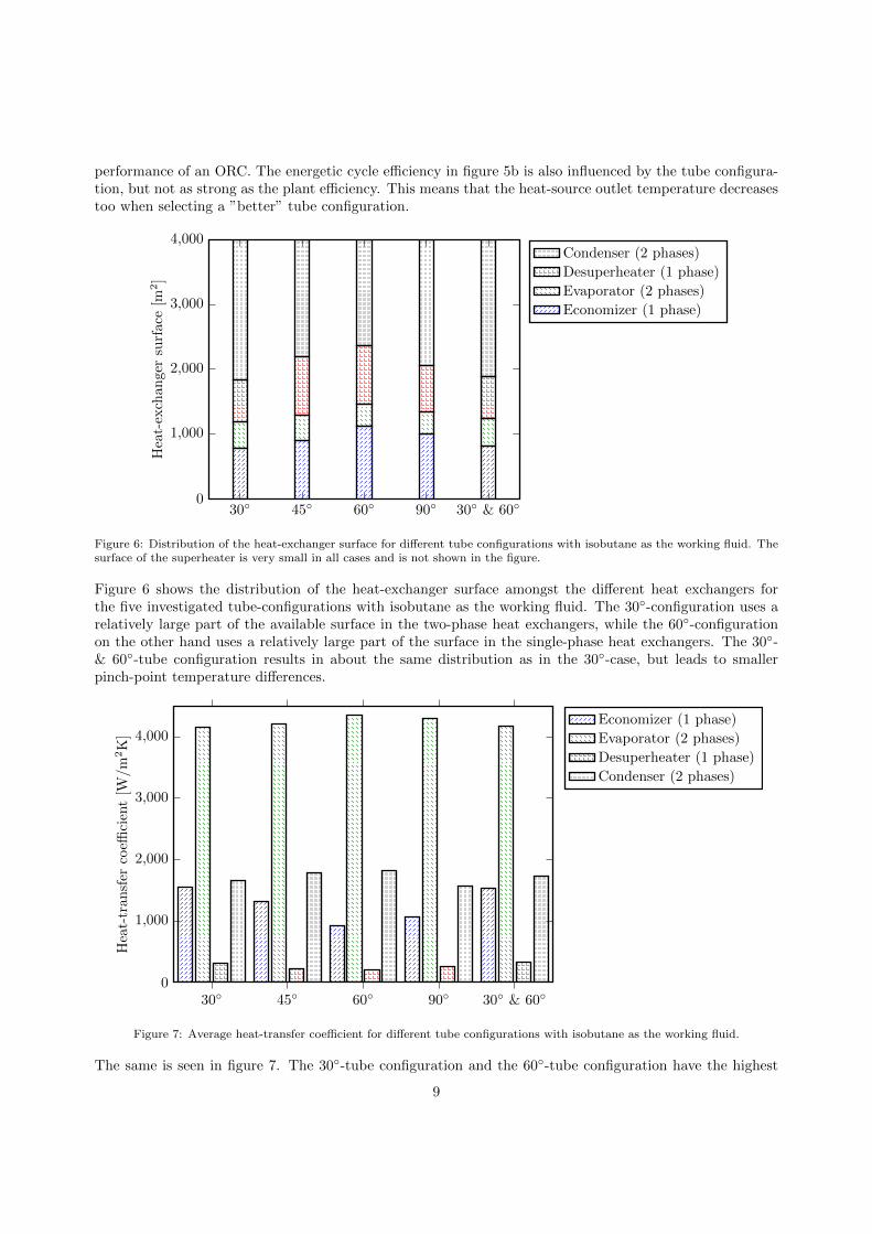
performance of an ORC. The energetic cycle efficiency in figure 5b is also influenced by the tube configura-tion, but not as strong as the plant efficiency. This means that the heat-source outlet temperature decreasestoo when selecting a ”better” tube configuration.

30◦ 45◦ 60◦ 90◦ 30◦ & 60◦0

1,000

2,000

3,000

4,000

Heat-exchanger

surface

[m2]

Condenser (2 phases)

Desuperheater (1 phase)

Evaporator (2 phases)

Economizer (1 phase)

Figure 6: Distribution of the heat-exchanger surface for different tube configurations with isobutane as the working fluid. Thesurface of the superheater is very small in all cases and is not shown in the figure.

Figure 6 shows the distribution of the heat-exchanger surface amongst the different heat exchangers forthe five investigated tube-configurations with isobutane as the working fluid. The 30◦-configuration uses arelatively large part of the available surface in the two-phase heat exchangers, while the 60◦-configurationon the other hand uses a relatively large part of the surface in the single-phase heat exchangers. The 30◦-& 60◦-tube configuration results in about the same distribution as in the 30◦-case, but leads to smallerpinch-point temperature differences.

30◦ 45◦ 60◦ 90◦ 30◦ & 60◦0

1,000

2,000

3,000

4,000

Hea

t-tr

ansf

erco

effici

ent

[W/m

2K

]

Economizer (1 phase)

Evaporator (2 phases)

Desuperheater (1 phase)

Condenser (2 phases)

Figure 7: Average heat-transfer coefficient for different tube configurations with isobutane as the working fluid.

The same is seen in figure 7. The 30◦-tube configuration and the 60◦-tube configuration have the highest

9

average heat-transfer coefficient in the single-phase heat exchangers and the two-phase heat exchangers,respectively, for isobutane. Combining these two (mono-layout) tube configurations for different heat ex-changers results in relatively high heat transfer coefficients in all heat exchangers.

For stand-alone shell-and-tube heat exchangers, it is common practice to select the 30◦-tube configura-tion for the single-phase heat exchangers and to select the 60◦-tube configuration for phase-change flow[17, 18]. The foregoing results show that the experience with the tube configuration of stand-alone exchang-ers is also valid for heat exchangers in an ORC.

The 30◦- & 60◦-tube configuration performs the best for all fluids and will be used in the remainder ofthis paper.

Figure 8 shows the exergetic plant, the net power output and energetic cycle efficiency for single- anddouble-pressure ORCs. Both use the 30◦-tube configuration and the 60◦-tube configuration for the single-phase and two-phase heat exchangers, respectively. The plant efficiency of subcritical cycles (isobutane,propane, R134a, R245fa and RC318) can increase strongly by adding a second pressure level. The extrapressure level has a limited effect for transcritical cycles. These transcritical cycles are outperformed by thedual-pressure subcritical ones.

Isob

utane

Propan

e

R134a

R218

R227ea

R245fa

R1234yf

RC318

30

35

40

45

2.2

2.4

2.6

2.8

3

ηplant

ex

[%]

Electricalpow

er[M

W]

1 pressure 2 pressures

(a) Exergetic plant efficiency

Isob

utane

Propan

e

R134a

R218

R227ea

R245fa

R1234yf

RC318

7

8

9

10

11

12ηcycle

en

[%]

1 pressure 2 pressures

(b) Energetic cycle efficiency

Figure 8: Exergetic plant efficiency and electrical power output (a) and energetic cycle efficiency (b) for single-pressure anddouble-pressure, simple ORCs with all shell-and-tube heat exchangers for different fluids. Single-phase heat exchangers use the30◦-tube configuration and the two-phase heat exchangers use the 60◦-tube configuration.

The energetic cycle efficiency (see figure 8b) does not increase or even decreases by adding an extra pressurelevel. This means that the increase of the plant efficiency results from a decrease in the heat-source outlettemperature, which is seen in figure 9. The outlet temperature can decrease almost 10◦C for subcriticalcycles, while the decrease is limited for transcritical cycles.

5.3. Constrained heat-source outlet temperature

It is possible to use the heat source for both electricity production and useful heat delivery. When a seriesconfiguration is used, the temperature of the heat source after the ORC has to be warm enough to deliver the

10

Isobutane

Propane

R134a

R218

R227ea

R245fa

R1234yf

RC318

50

55

60

65

70

Outlet

temperature

[◦C]

1 pressure 2 pressures

Figure 9: Heat-source outlet temperature for single-pressure and double-pressure simple ORCs with all shell-and-tube heatexchangers for different fluids. The transcritical cycles are the ones with R218, R227ea and R1234yf.

heat. In this section the heat-source outlet temperature is constrained and the influence on the performanceof the power plant is investigated.

Isob

utane

Propan

e

R134a

R218

R227ea

R245fa

R1234yf

RC318

20

30

40

50

1.5

2

2.5

3

3.5

ηplant

ex

[%]

Electricalpow

er[M

W]

Simple-70◦C Recuperated-70◦CSimple-90◦C Recuperated-90◦C

(a) Exergetic plant efficiency

Isob

utane

Propan

e

R134a

R218

R227ea

R245fa

R1234yf

RC318

8

10

12

14

ηcycle

en

[%]

Simple-70◦C Recuperated-70◦CSimple-90◦C Recuperated-90◦C

(b) Energetic cycle efficiency

Figure 10: Exergetic plant efficiency and electrical power output (a) and energetic cycle efficiency (b) for single-pressure,simple and recuperated ORCs with all shell-and-tube heat exchangers for different fluids. The heat source outlet temperatureis constained to 70 or 90◦C.

Figure 10a shows the exergetic plant efficiency and net power output for both simple and recuperatedcycles when the minimum heat-source outlet temperature is 70 or 90◦C. The plant efficiency increases inmost cases by adding a recuperator. The higher the required heat source outlet temperature, the higher is

11

the effect of the recuperator. The plant efficiency is of course higher when the constraint on the heat sourceoutlet temperature is lower.

Because of the internal heat recuperation in the recuperated cycle, less heat is added to the cycle andthe cycle efficiency is higher than in the simple cycle. This is seen in figure 10b. When the heat sourceoutlet temperature is limited to 90◦C, the cycle efficiency is (much) higher than in the case of a 70◦C-limitfor both the simple and recuperated cycle. When the heat source outlet temperature increases, the heatsource cooling efficiency decreases and the optimizer chooses to increase the cycle efficiency in order to limitthe decrease of the plant efficiency.

6. Conclusions

The system optimization of different configurations of ORCs with shell-and-tube heat exchangers is per-formed in this paper. Models for heat exchangers used in single-phase flow, evaporation and condensationwhich are available in the literature are implemented and added to a previously developed ORC-model.The configuration of all heat exchangers and the cycle parameters are optimized together. The total heat-exchanger surface of all heat exchangers together is constrained in order to avoid an unrealistically largeand expensive power plant.

Five different tube configurations are compared to each other. If all heat exchangers should have thesame tube configuration, it is best to use the 30◦-tube configuration. An efficiency improvement can beobtained by applying the 30◦-tube configuration and the 60◦-tube configurations in the single-phase andtwo-phase heat exchangers, respectively.

The plant efficiency of subcritical, single-pressure cycles can increase strongly by adding a second pres-sure level. This increase is induced by a decrease of the heat-source outlet temperature. The cycle efficiencyremains about constant.

It is also shown that recuperated cycles are only useful when the heat-source outlet temperature is con-strained. The higher the heat-source outlet temperature has to be, the higher the effect of recuperation. Anincrease in the heat-source outlet temperature results, both for simple and recuperated cycles, in a highercycle efficiency. Due to the constraint on the heat-source outlet temperature, the heat-source cooling effi-ciency is limited and the only way to adapt the plant efficiency is by adapting the cycle efficiency.

Future steps in this research will be to include more components and to go towards an economic systemoptimization.

12

Nomenclature

Greek

δ Clearance [m]∆p Pressure drop [Pa]∆T Temperature difference [◦C]η Efficiency [-]µ Dynamic viscosity [Pa s]ρ Density [kg/m3]θ Angle [◦]ζ Correction factor for non-ideality in pressure drop [-]

13

Roman

A Area [m2]cp Specific eat capacity [J/kgK]do Tube outside diameter [m]D Diameter [m]e Specific exergy [kJ/kg]F Fraction of number of tubes [-]G Mass velocity [kg/m2s]h Heat transfer coefficient [W/m2K]

Specific enthalpy [J/kg]Hg Hagen number [-]J Correction factor for non-ideality in heat transfer [-]lc Baffle cut length [m]Lb Baffle cut length [m]Li Tube length of part i [m]Lq Leveque number [-]m Mass flow [kg/s]Nb Number of baffles [-]Nt Number of tubes [-]Nu Nusselt number [-]p Pressure [bar]Pr Prandtl number [-]pt Tube pitch [m]

Q Heat flow [kW]Re Reynolds number [-]T Temperature [◦C]

W Mechanical power [kW]X Tube pitch [m]Y 2 Chisholm parameter [-]

14

Sub-and superscripts

0 Dead state1− 9 Number of the stateac Accelerationc Centercr Crossflowctl Center outermost tubescycle Cycleen Energeticex Exergeticfr Frictionalh Hydraulicid Idealin Inletmax Maximummin Minimumnet Nettl Longitudinalotl Outermost tubesout Outletplant Plants Shellsource Heat sourcet Transversetot Totalw Window flowwf Working fluid

Acknowledgments

Daniel Walraven is supported by a VITO doctoral grant. The valuable discussions on optimization withJoris Gillis (KU Leuven) are gratefully acknowledged and highly appreciated.

References

[1] J. Tester, B. Anderson, A. Batchelor, D. Blackwell, R. DiPippo, E. Drake, J. Garnish, B. Livesay, M. Moore, K. Nichols,The Future of Geothermal Energy: Impact of Enhanced Geothermal Systems (EGS) on the United States in the 21stCentury, Tech. Rep., Massachusetts Institute of Technology, Massachusetts, USA, 2006.

[2] Y. Dai, J. Wang, L. Gao, Parametric optimization and comparative study of organic Rankine cycle (ORC) for low gradewaste heat recovery, Energy Conversion and Management 50 (3) (2009) 576–582.

[3] B. Saleh, G. Koglbauer, M. Wendland, J. Fischer, Working fluids for low-temperature organic Rankine cycles, Energy32 (7) (2007) 1210–1221.

[4] D. Walraven, B. Laenen, W. Dhaeseleer, Comparison of thermodynamic cycles for power production from low-temperaturegeothermal heat sources, Energy Conversion and Management 66 (2013) 220–233.

[5] D. Wei, X. Lu, Z. Lu, J. Gu, Performance analysis and optimization of organic Rankine cycle (ORC) for waste heatrecovery, Energy conversion and Management 48 (4) (2007) 1113–1119.

[6] B. Babu, S. Munawar, Differential evolution strategies for optimal design of shell-and-tube heat exchangers, ChemicalEngineering Science 62 (14) (2007) 3720–3739.

[7] B. Allen, L. Gosselin, Optimal geometry and flow arrangement for minimizing the cost of shell-and-tube condensers,International Journal of Energy Research 32 (10) (2008) 958–969.

[8] A. L. Costa, E. M. Queiroz, Design optimization of shell-and-tube heat exchangers, Applied Thermal Engineering 28 (14)(2008) 1798–1805.

15

[9] V. Patel, R. Rao, Design optimization of shell-and-tube heat exchanger using particle swarm optimization technique,Applied Thermal Engineering 30 (11) (2010) 1417–1425.

[10] L. Wang, B. Sunden, Optimal design of plate heat exchangers with and without pressure drop specifications, AppliedThermal Engineering 23 (3) (2003) 295–311.

[11] J. Zhu, W. Zhang, Optimization design of plate heat exchangers (PHE) for geothermal district heating systems, Geother-mics 33 (3) (2004) 337–347.

[12] A. Conradie, J. Buys, D. Kroger, Performance optimization of dry-cooling systems for power plants through SQP methods,Applied thermal engineering 18 (1) (1998) 25–45.

[13] A. Doodman, M. Fesanghary, R. Hosseini, A robust stochastic approach for design optimization of air cooled heat ex-changers, Applied Energy 86 (7) (2009) 1240–1245.

[14] E. Rubio-Castro, M. Serna-Gonzalez, J. M. Ponce-Ortega, M. A. Morales-Cabrera, Optimization of mechanical draftcounter flow wet-cooling towers using a rigorous model, Applied Thermal Engineering 31 (16) (2011) 3615–3628.

[15] H. Madhawa Hettiarachchi, M. Golubovic, W. M. Worek, Y. Ikegami, Optimum design criteria for an organic Rankinecycle using low-temperature geothermal heat sources, Energy 32 (9) (2007) 1698–1706.

[16] A. Franco, M. Villani, Optimal design of binary cycle power plants for water-dominated, medium-temperature geothermalfields, Geothermics 38 (4) (2009) 379–391.

[17] G. F. Hewitt, Hemisphere handbook of heat exchanger design, Hemisphere Publishing Corporation New York, 1990.[18] R. K. Shah, D. P. Sekulic, Fundamentals of heat exchanger design, John Wiley and Sons, Inc., 2003.[19] T. Tinker, Shell side characteristics of shell and tube heat exchangers, General Discussion on Heat Transfer (1951) 89–116.[20] J. Andersson, J. Akesson, M. Diehl, CasADi – A symbolic package for automatic differentiation and optimal control, in:

S. Forth, P. Hovland, E. Phipps, J. Utke, A. Walther (Eds.), Recent Advances in Algorithmic Differentiation, vol. 87 ofLecture Notes in Computational Science and Engineering, Springer Berlin Heidelberg, 297–307, 2012.

[21] C. Buskens, D. Wassel, The ESA NLP Solver WORHP, in: Modeling and Optimization in Space Engineering, Springer,85–110, 2013.

[22] E. Lemmon, M. Huber, M. Mclinden, NIST Reference Fluid Thermodynamic and Transport Properties REFPROP, TheNational Institute of Standards and Technology (NIST), version 8.0, 2007.

[23] J. R. Martins, P. Sturdza, J. J. Alonso, The complex-step derivative approximation, ACM Transactions on MathematicalSoftware (TOMS) 29 (3) (2003) 245–262.

[24] P. Peterson, F2PY: a tool for connecting Fortran and Python programs, International Journal of Computational Scienceand Engineering 4 (4) (2009) 296–305.

[25] R. Mukherjee, Effectively design shell-and-tube heat exchangers, Chemical Engineering Progress 94 (2) (1998) 21–37.[26] B. Petukhov, V. Popov, Theoretical calculation of heat exchange and frictional resistance in turbulent flow in tubes of an

incompressible fluid with variable physical properties(Heat exchange and frictional resistance in turbulent flow of liquidswith variable physical properties through tubes), High Temperature 1 (1963) 69–83.

[27] M. Bhatti, R. Shah, Turbulent and transition convective heat transfer in ducts, in: S. Kakac, R. Shah, W. Aung (Eds.),Handbook of Single-Phase Convective Heat Transfer, chap. 4, Wiley, New York, 1987.

Appendix A. Geometry

The equations to calculate the important geometrical parameters of a shell-and-tube heat exchanger arestated in this section. More information can be found in the literature [17, 18], on which this section isbased.The diameter of the outermost tubes Dotl and the diameter of the circle through the center of the outermosttubes Dctl are given by:

Dotl = Ds − δbb, (A.1)

Dctl = Dotl − do, (A.2)

with δbb the diametrical shell-to-tube bundle bypass clearance, which can be estimated as δbb = 0.017Ds +0.0265 [m] [17]. The remaining two parameters in figure 2 are calculated as:

θb = 2 cos−1(

1− 2lcDs

), (A.3)

θctl = 2 cos−1(Ds − 2lcDctl

). (A.4)

The number of tubes Nt in a shell without impingement plates and a single tube pass is:

Nt =π/4D2

ctl

Ctp2t, (A.5)

16

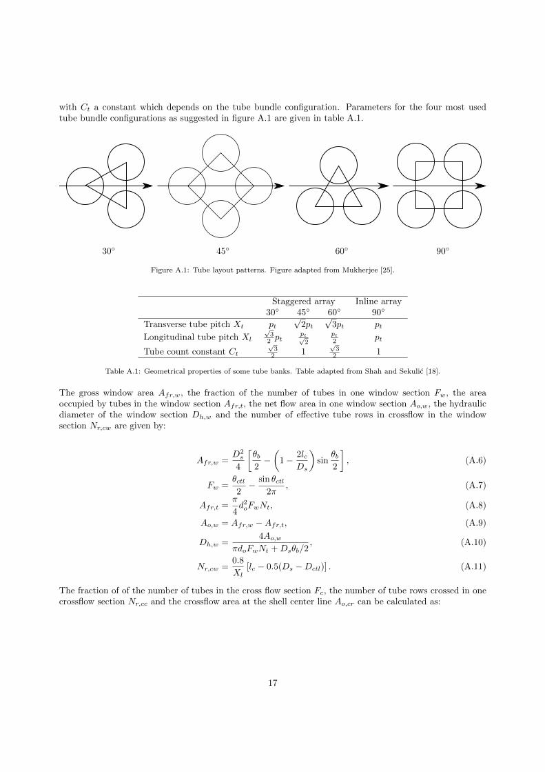
with Ct a constant which depends on the tube bundle configuration. Parameters for the four most usedtube bundle configurations as suggested in figure A.1 are given in table A.1.

90◦45◦ 60◦30◦

Figure A.1: Tube layout patterns. Figure adapted from Mukherjee [25].

Staggered array Inline array30◦ 45◦ 60◦ 90◦

Transverse tube pitch Xt pt√

2pt√

3pt pt

Longitudinal tube pitch Xl

√32 pt

pt√2

pt2 pt

Tube count constant Ct√32 1

√32 1

Table A.1: Geometrical properties of some tube banks. Table adapted from Shah and Sekulic [18].

The gross window area Afr,w, the fraction of the number of tubes in one window section Fw, the areaoccupied by tubes in the window section Afr,t, the net flow area in one window section Ao,w, the hydraulicdiameter of the window section Dh,w and the number of effective tube rows in crossflow in the windowsection Nr,cw are given by:

Afr,w =D2s

4

[θb2−(

1− 2lcDs

)sin

θb2

], (A.6)

Fw =θctl2− sin θctl

2π, (A.7)

Afr,t =π

4d2oFwNt, (A.8)

Ao,w = Afr,w −Afr,t, (A.9)

Dh,w =4Ao,w

πdoFwNt +Dsθb/2, (A.10)

Nr,cw =0.8

Xl[lc − 0.5(Ds −Dctl)] . (A.11)

The fraction of of the number of tubes in the cross flow section Fc, the number of tube rows crossed in onecrossflow section Nr,cc and the crossflow area at the shell center line Ao,cr can be calculated as:

17

Fc = 1− 2Fw, (A.12)

Nr,cc =Ds − 2lcXl

, (A.13)

Ao,cr =

[Ds −Dotl +

Dctl

Xt(Xt − do)

]Lb,c, (A.14)

Ao,cr =

[Ds −Dotl + 2

Dctl

Xt(pt − do)

]Lb,c. (A.15)

The first expression for Ao,cr is valid for 30◦- and 90◦-tube configurations and for 45◦- and 60◦-tube configura-tions with a high pitch. The second expression is valid for 45◦- and 60◦-tube configurations with a low pitch.

The flow area for bypass stream C (section 3.2) Fbp, the total tube-to-baffle leakage area for one baffleAo,tb and the shell-to-baffle leakage area Ao,sb are given by:

Fbp =(Ds −Dotl)Lb,c

Ao,cr, (A.16)

Ao,tb =π

4

[(do + δtb)

2 − d2o]Nt(1− Fw), (A.17)

Ao,sb = πDsδsb2

(1− θb

2π

), (A.18)

with δtb = 0.4 10−3 [m] the diametrical clearance and δsb = 3.1 10−3 + 0.004Ds [m] the shell-to-baffleclearance as given by TEMA standards [17].

Appendix B. Heat transfer and pressure drop

B.1. Single-phase flow

B.1.1. Shell side

The ideal heat transfer coefficient on the shell-side in inline tube bundles (90◦ configurations) is given by[18]:

hid,shellsingle =k

Dh0.404Lq1/3

(Red + 1

Red + 1000

)0.1

, (B.1)

Lq = 1.18Hg Pr

((4X∗t /π)− 1

X∗l

), (B.2)

Hg = Hglam +Hgturb,i

[1− exp

(1− Red + 1000

2000

)], (B.3)

Hglam = 140Red(X∗l

0.5 − 0.6)2 + 0.75

X∗t1.6(4X∗tX

∗l /π − 1)

, (B.4)

Hgturb,i =

[(0.11 +

0.6(1− 0.94/X∗l )0.6

(X∗t − 0.85)1.3

)100.47(X

∗l /X

∗t −1.5) + 0.015(X∗t − 1)(X∗l − 1)

]×Re2−0.1(X

∗l /X

∗t )

d + φt,nRe2d, (B.5)

um = u∞X∗t

X∗t − 1, (B.6)

18

with k the thermal conductivity of the fluid, Lq the Leveque number, Hg the Hagen number, Pr the Prandtlnumber, u∞ the free stream velocity, φt,n a correction factor for tube bundle inlet and outlet pressure dropsand Red the Reynolds number in the shell. These last two parameters are calculated as:

φt,n =

1

2X∗t2

(1Nr− 1

10

)for 5 ≤ Nr ≤ 10 and X∗l ≥ 0.5(2X∗t + 1)1/2

2[

X∗d−1

X∗t (X

∗t −1)

]2 (1Nr− 1

10

)for 5 ≤ Nr ≤ 10 and X∗l < 0.5(2X∗t + 1)1/2

0 for Nr > 10

, (B.7)

Red =ρumdoµ

. (B.8)

X∗l , X∗t and X∗d are dimensionless parameters, obtained by dividing Xl, Xt and Xd =√X2l +X2

t by do,respectively. ρ is the density and µ the dynamic viscosity.For staggered tube bundles (30, 45 and 60◦ configurations), the correlations are [18]:

hid,shellsingle =k

Dh0.404Lq1/3, (B.9)

Lq =

0.92Hg Pr(

(4X∗t /π)−1X∗

d

)for X∗l ≥ 1

0.92Hg Pr(

(4X∗tX

∗l /π)−1

X∗l X

∗d

)for X∗l < 1

, (B.10)

Hg = Hglam +Hgturb,s

[1− exp

(1− Red + 200

1000

)], (B.11)

Hglam =

140Red(X∗

l0.5−0.6)2+0.75

X∗t1.6(4X∗

tX∗l /π−1)

for X∗l ≥ 0.5(2X2t + 1)1/2

140Red(X∗

l0.5−0.6)2+0.75

X∗d1.6(4X∗

tX∗l /π−1)

for X∗l < 0.5(2X2t + 1)1/2

, (B.12)

Hgturb,s =

[(1.25 +

0.6

(X∗t − 0.85)1.08

)+ 0.2

(X∗lX∗t− 1

)3

− 0.005

(X∗tX∗l− 1

)3]

×Re1.75d + φt,nRe2d, (B.13)

Hgturb,s,corr = Hgturb,s

(1 +

Red − 250 000

325 000

), (B.14)

um =

{u∞

X∗t

X∗t −1 for X∗l ≥ 0.5(2X∗t + 1)1/2

u∞X∗

t

2(X∗d−1)

for X∗l < 0.5(2X∗t + 1)1/2. (B.15)

The pressure drop in an ideal crossflow section ∆pb,id between two baffles and in an ideal window flow ∆pw,idare given by:

∆pb,id =µ2

ρ

Nr,ccd2o

Hg, (B.16)

∆pw,id =

(2 + 0.6Nr,cw)G2

w

2ρ for Red > 10026Gwµρ

(Nr,cw

pt−do + Lb

D2h,w

)+

G2w

ρ for Red ≤ 100, (B.17)

with Gw the mass velocity in the window section:

Gw =m√

Ao,crAo,w, (B.18)

and m the mass flow of the fluid. The hydrostatic pressure drop is neglected because the shell-side fluid flowsalternately up and down and the hydrostatic pressure drop is therefore alternately positive and negative.Both are about equal and can therefore be neglected.

19

B.1.2. Tube side

The correlation of Petukhov and Popov [26] is used to calculate the single phase heat transfer coefficient inthe tubes. The friction coefficient is calculated by the correlation of Bhatti and Shah [27].

B.2. Heat transfer and pressure drop while evaporating

The boiling heat transfer coefficient for evaporation on the shell-side is given by [17]:

hid,shellevap = hnbFb + hnc, (B.19)

with hnb the nucleate boiling coefficient, Fb a correction factor for the effect of convection and hnc the naturalconvection heat transfer coefficient, which is about 250 W/m2K for hydrocarbons. The other parametersare given as [17]:

hnb = 0.00417p0.69crit q0.7Fp, (B.20)

Fp = 0.7 + 2pr

(4 +

1

1− pr

), (B.21)

Fb = 1 + 0.1

[0.785Dotl

Ct(pt/do)2do− 1

]0.75, (B.22)

where pcrit is the critical pressure of the fluid, q the heat flux and pr = p/pcrit the reduced pressure.The frictional, ideal pressure drop is given as [17]:

fr∆pid,shellevap =(

1 + (Y 2 − 1)[Bx(2−n)/2(1− x)(2−n)/2 + x2−n

])frlo

∆pid,shellsingle (B.23)

where frlo ∆pshellsingle is the frictional, ideal pressure drop in the shell if all the fluid was saturated liquid,

Y 2 =frlo ∆pshellid,single/

frvo∆pid,shellsingle the Chisholm parameter and x the quality of the fluid. For the cross flow

B = 1 and n = 0.37, while for the window flow B = (ρh/ρl)1/4 and n = 0. ρh is the homogeneous flow

density, given as:

ρh =1

1−xρl

+ xρv

(B.24)

The subscripts l and v refer to saturated liquid and vapor, respectively.The acceleration pressure drop is [17]:

ac∆pid,shellevap = G2

((1− x)2

ρl(1− α)+

x2

ρvα

)out

−(

(1− x)2

ρl(1− α)+

x2

ρvα

)in

, (B.25)

with α = 1/(1 + 1−xx

ρvρl

) the void fraction as calculated for a homogeneous flow [17].

B.3. Heat transfer and pressure drop while condensing

The heat transfer coefficient for condensation on the shell-side is given by [17]:

hid,shellcond =k

doK(χ4Re2lv +Nu4f

)1/4, (B.26)

20

with

Nu4f = 0.276

[d3oρl(ρl − ρv)g(hv − hl)

µlkl(Tsat − Tw)

], (B.27)

χ = 0.9

(1 +

1

RH

)1/3

, (B.28)

R =

(ρlµlρgµg

)1/2

, (B.29)

H =cp,l(Tsat − Tw)

Prl(hv − hl), (B.30)

Relv =do

mxLbcDs

ρl

µlρv, (B.31)

where h is the specific enthalpy and cp the heat capacity at constant pressure. The two-phase pressure dropis calculated by the same correlations as given for the evaporator.

21