optimum acquisition and processing parameters for
TRANSCRIPT

Scholars' Mine Scholars' Mine
Masters Theses Student Theses and Dissertations
Summer 2015
Optimum acquisition and processing parameters for multichannel Optimum acquisition and processing parameters for multichannel
analysis of surface waves using 3D electrical resistivity analysis of surface waves using 3D electrical resistivity
tomography as control tomography as control
Uchenna Chibuzo Nwafor
Follow this and additional works at: https://scholarsmine.mst.edu/masters_theses
Part of the Geological Engineering Commons
Department: Department:
Recommended Citation Recommended Citation Nwafor, Uchenna Chibuzo, "Optimum acquisition and processing parameters for multichannel analysis of surface waves using 3D electrical resistivity tomography as control" (2015). Masters Theses. 7437. https://scholarsmine.mst.edu/masters_theses/7437
This thesis is brought to you by Scholars' Mine, a service of the Missouri S&T Library and Learning Resources. This work is protected by U. S. Copyright Law. Unauthorized use including reproduction for redistribution requires the permission of the copyright holder. For more information, please contact [email protected].

OPTIMUM ACQUISITION AND PROCESSING PARAMETERS FOR
MULTICHANNEL ANALYSIS OF SURFACE WAVES USING 3 D
ELECTRICAL RESISTIVITY TOMOGRAPHY AS CONTROL
by
UCHENNA CHIBUZO NWAFOR
A THESIS
Presented To the Faculty of Graduate School of the
MISSOURI UNIVERSITY OF SCIENCE AND TECHNOLOGY
In Partial Fulfillment of the Requirements for the Degree
MASTER OF SCIENCE
IN
GEOLOGICAL ENGINEERING
2015
Approved
Neil Anderson, Advisor
J. David Rogers
Maochen Ge

iii
ABSTRACT
Multichannel Analysis of Surface Waves (MASW) and Electrical Resistivity
Tomography (ERT) data were acquired in the Newburg, Missouri with the goal of
determining optimum MASW acquisition parameters. Users of the MASW tool
generally state that greater geophone intervals and greater shot-to-receiver offsets provide
for more accurate results. The objective was to determine if this “rule of thumb” applies
in karst terrain.
ERT data were acquired along four traverses with eighty-four (84) electrodes at
five feet spacing with SuperSting R8 Resistivity System using dipole- dipole array. The
data were processed using Earth Imager to generate 2-D resistivity inversion and
thereafter, Voxler software was used to collate the 2-D ERT data into a 3-D resistivity
model. MASW data on the other hand, were acquired along the same ERT traverses on
the same locations using a suite of different geophone intervals (1-ft, 2.5-ft, 5-ft, 7.5-ft,
and 10-ft) and shot-to-receiver spacings (0-ft, 10-ft, 20-ft, 30-ft, 40-ft, and 50-ft) with a
20lb sledge hammer as the source. The data were processed using Surfseis software to
generate the dispersion curves and 1-D shear wave velocity profiles of the area.
On the basis of the comparative analyses of the ERT and MASW data, it was
determined that 2.5-ft and 5-ft geophone gave generated depth of bedrock that was
consistent with ERT data. With 5-ft geophone spacing it is possible to image the
subsurface to greater depth, but with the 7.5-ft and 10-ft, unidentifiable dispersion curves
would be generated. Therefore, in this study area, on the basis of data that were acquired
it is recommended that 2.5ft spacing be used if depth of investigation is about 40ft, but if
the depth of investigation is about 80-ft, using a sledge hammer source then 5-ft
geophone spacing at 20-ft shot-receiver offset distance is recommended.

iv
ACKNOWLEDGEMENT
I would like to thank my advisor Dr. Neil Anderson for his encouragement and
support during the period of this research. Also, my appreciation goes to members of the
committee; Dr. J. David Rogers and Dr. Maochen Ge, for their time and participation in
the completion of this project.
The completion of this thesis would not have been possible without the
corroborative efforts of several individuals. The following individuals have contributed
time and resources to the completion of this study: Stanley Nwokebuihe, Rafael Araujo,
and Dennis Duru.
I would like to thank Mr. Ben and his family for providing us with their farm sites
to carry out this research.
Specifically, I would like to thank my wife Miss Ebere Nwafor, for her patience
and support throughout my graduate study years, Ebere you have been a great wife.
This work is dedicated to my loving wife, Ebere. Without your love and sacrifice,
I would not be achieving this milestone.
Thank you.

v
TABLE OF CONTENTS
Page
ABSTRACT ………………………………………………………………………..….iii
ACKNOWLEDGEMENT …………………………………………………………...…iv
LISTS OF FIGURES ……………………………………………………………….....ix
LISTS OF TABLES …………………………………………………………...………xii
SECTION
1. INTRODUCTION ……………………………………………………………………..1
1.1 OBJECTIVES ………………………………………………………………….......2
1.2 ORGANIZATION ……………………………………………………………..…3
2. OVERVIEWS OF MULTICHANNEL ANALYSIS OF SURFACE WAVES ……….4
2.1 INTRODUCTION …………………………………………………………………4
2.2 BASIC WAVE THEORY ………………………………………………………….4
2.2.1 Body Waves and Surface Waves ………………………………………….....8
2.2.2 Rayleigh Waves Velocity …………………………………………………..12
2.2.3 Relationship between Shear Waves and Soil/Rock Conditions …………….13
2.3 MULTICHANNEL ANALYSIS OF SURFACE WAVES METHOD…………...15
2.3.1 Overview ………………………………………………….………………..17
2.3.2 MASW Using Impulsive Source (MASWI) ………………………………...19
2.4 MASW EQUIPMENT ………………………………………………………...…21
2.4.1 Seismic Source ……………………………………………………………...21
2.4.2 Trigger Mechanism …………………………………………………………..22
2.4.3 Geophones …………………………………………………………………....23

vi
2.4.4 Geophone Cable …………………………………………………………….24
2.4.5 Seismograph ………………………………………………………………...25
2.5 MASW FIELD SURVEY SETUP ……………………………………………….25
2.5.1 Overviews of MASW Data Acquisition ……………………………………26
2.5.2 Overviews of Data Processing ……………………………………………...27
3. OVERVIEWS OF ELECTRICAL RESISTIVITY TOMOGRAPHY METHOD……31
3.1 INTRODUCTION ………………………………………………………………..31
3.2 BASIC THEORY ………………………………………………………………...32
3.3 ARRAYS …………………………………………………………………………37
3.4 RELATIONSHIP BETWEEN RESISTIVITY AND SOIL/ROCK
CONDITION……………………………………………………………………..39
3.4.1 Overviews of Two-Dimensional Electrical Resistivity Surveying …….…..40
3.4.2 Three-Dimensional Electrical Resistivity Surveying (3-D) ………………..42
3.5 FIELD EQUIPMENT …………………………………………………………….43
3.5.1 Transmitter/Receiver ………………………………………………………..43
3.5.2 Cables ……………………………………………………………………….44
3.5.3 Current and Potential Electrodes …………………………………………...44
3.5.4 Power Source ……………………………………………………………….45
3.6 OVERVIEW OF ERT DATA ACQUISITION …………………………………..45
3.7 DATA PROCESSING AND INTERPRETATION ………………………………47
4. RESEARCH METHODS …………………………………………………………….50
4.1 OVERVIEW ……………………………………………………………………...50
4.2 SITE LOCATION ………………………………………………………………...50

vii
4.3 MASW TESTING ………………………………………………………………..55
4.3.1 Site Setup ……………………………………………………………...........55
4.3.2 Field Procedures and Equipment …………………………………………...57
4.3.3 Data Acquisition ……………………………………………………………59
4.3.4 Data Processing and Inversion ……………………………………………...68
4.4 ELECTRICAL RESISTIVITY TOMOGRAPHY (ERT) ………………………..85
4.4.1 Site Setup ……………………………………………...................................85
4.4.2 Field Procedures and Equipment …………………………………………...87
4.4.3 Data Acquisition ……………………………………………………………89
4.4.4 Data Processing and Inversion ……………………………………………...91
4.5 CONCLUSIONS …………………………………………………………………98
5. RESULTS …………………………………………………………………………….99
5.1 OVERVIEW ……………………………………………………………………...99
5.2 RESULTS FROM MASW DATA …………………………………………….....99
5.3 RESULTS FROM ERT DATA …………………………………………………106
5.4 MUTING ………………………………………………………………...............109
5.4.1 Results from Muting ………………………………………………………113
5.4.2 Importance of Muting ……………………………………..........................114
6. DISCUSSIONS ……………………………………………………………………...115
6.1 OVERVIEW …………………………………………………………………….115
6.2 COMPARISON OF MASW RESULTS WITH 2-D ERT RESULTS…………..115
6.3 FINAL ANALYSIS ……………………………………………………………..124
7. CONCLUSIONS ………………………………...………………………………….125

viii
8. RECOMMENDATIONS…………………………………………………………….127
BIBIOGRAPHY………………………………………………………………………..128
VITA …………………………………………………………………………………...131

ix
LISTS OF FIGURES Page
Figure 2.1: Bulk modulus equations and calculations …………………………………...6
Figure 2.2: Showing how to determine and calculate shear modulus …………………….7
Figure 2.3: Diagram showing stress and strain relationship ……………………………...7
Figure 2.4: How P-waves and S- waves travel through a medium………………………..9
Figure 2.5: Block models of mode of propagation for Love waves and Rayleigh
waves……………………………………………………………………………………..12
Figure 2.6: Showing typical MASW field setup ………………………………………..19
Figure 2.7: Showing typical MASWV field setup ………………………………………19
Figure 2.8: Showing typical MASWI field setup………………………………………..21
Figure 2.9: Showing different array configurations for the MASWP ………………….21
Figure 2.10: Example of Sledgehammer Triggering Device…………………………….23
Figure 2.11: Example of spike-coupled Geophone ……………………………………..24
Figure 2.12: Instrumentation of MASW Tomography Survey …………………………26
Figure 2.13: Progression of MASW Tomography Survey ……………………………...27
Figure 2.14: Processing Steps to Estimate Shear Wave Velocity ……………………….28
Figure 3.1: Equipotential and current lines for a pair of current electrodes
A and B on a homogeneous half-space. ……………………………………………..…..35
Figure 3.2: Electrode array configurations for resistivity measurements ………………38
Figure 3.3: Two-dimensional measurement configurations for a dipole-dipole
resistivity profile, pseudosection plotting location indicated in red……………...…..…41
Figure 3.4: Examples of measured apparent resistivity, calculated apparent
resistivity, and inverted resistivity…………………………………………….………...42
Figure 3.5: Example of Developed Psuedosection Model Using a Wenner Array
and 28 Electrodes………………………………………………………………...............47
Figure 3.6: Flow Chart of Resistivity Inversion Processing…………………………….49

x
Figure 4.1: Newburg map showing the study area located within Mark Twain
National Forest…...............................................................................................................50
Figure 4.2: Showing the location of Corn Creek Road …………………………………51
Figure 4.3: Alluvium and Surficial geology map of Newburg area……………………..52
Figure 4.4: Bedrock Geologic map of the study area…………………………………..53
Figure 4.5: MASW traverses (blue lines) oriented NE-SW and NE-NW and
ERT lines (red lines) oriented NW-SE………………………………..………………...55
Figure 4.6: 4.5 Hz Geophones with spikes........................................................................56
Figure 4.7: Showing cable (red), connectors (yellow), knob (black) and geophones
with spike…………………………………………………………………..………….....56
Figure 4.8: A one square foot metal plate………………………………………………..58
Figure 4.9: Shot gather for each of the array record at different offset distances….........60
Figure 4.10: A flowchart detailing the processing steps used for analyzing MASW
profiles (Kansas Geological Survey, 2014). ……………………………………….......68
Figure 4.11: All the generated dispersion curves and the inverted shear wave
velocity model for the different tests …………………………………………………...70
Figure 4.12: Switch box and SuperSting ………………………………………………..86
Figure 4.13: Four ERT traverses (red) and two MASW traverses (blue)………………..87
Figure 4.14: SuperSting Manager App, Plot pseudo section…………………………….89
Figure 4.15: Equipment set up for the ERT acquisition………………………………...90
Figure 4.16: Pseudo sections and data points generated for the ERT traverses...…….....92
Figure 4.17: Final inverted section for the resistivity analysis…………..………………94
Figure 4.18: 3-D ERT Model generate with Voxler software………………………......96
Figure 5.1: Final inverted section for the resistivity analysis for ERT line 1
showing top of bedrock in black dotted lines, pockets of consolidated
sand layer, moist soil and very intact bedrock……………………………………..…...107

xi
Figure 5.2: Final inverted section for the resistivity analysis for ERT line 2
showing top of bedrock in black dotted lines, pockets of consolidated
sand layer, moist soil and very intact bedrock……………………………………..…...108
Figure 5.3: Final inverted section for the resistivity analysis for ERT line 3
showing top of bedrock in black dotted lines, pockets of consolidated
sand layer, moist soil and very intact bedrock……………………………………….....108
Figure 5.4: Final inverted section for the resistivity analysis for ERT line 4
showing top of bedrock in black dotted lines, pockets of consolidated
sand layer, moist soil and very intact bedrock………………………………………....109
Figure 5.5: 3-D model generated by combining the four ERT traverses
using Voxler software…………………………………………..………………………109
Figure 5.6: Raw shot gather from a 2.5-ft geophone spacing and 0-ft receiver
offset before and after muting…………………………..................................................111
Figure 5.7 Dispersion curve for 2.5-ft spacing and 0-ft offset………………………….112

xii
LISTS OF TABLES
Page
Table 5.1: Results from all the dispersion curves and generated shear wave
velocity profiles…………………………………………………………………..…….106
Table 6.1: Final result analysis for MASW and ERT testing…………………………..124

1. INTRODUCTION
When important structures are built in active seismic zones or when the dynamic
properties of a soil are of interest, testing of the in-situ soil is required to determine its
shear wave velocity. The shear wave velocity of the soil is directly related to its shear
modulus and the shear modulus of the soil strongly influences how it will react during
dynamic loading. Several methods are available to measure the in-situ shear wave
velocity profile of a site. The simplest and most accurate methods are borehole seismic
methods, but these methods are also fairly expensive due to the need to drill boreholes
down to the desired depth of investigation. To reduce the cost and testing time associated
with borehole techniques, non-intrusive surface wave methods have been developed.
These methods are often significantly cheaper, faster, and easier to use and are
subsequently replacing borehole methods for many shear wave velocity investigations.
Various surface wave methods have been developed over the years to estimate the
in-situ shear wave velocity profile. The most common method used today is the multi-
channel analysis of surface waves (MASW). The MASW method is a newer technique
that has several different ways to collect and analyze data. Because there are several
different ways to collect and analyze the data, there are limited guidelines on receiver
positioning, source placement and source type that are most effective at producing
accurate results.
The purpose of this research is to determine the optimum acquisition and
processing parameter for MASW method on alluvium deposited site in Newburg,
Missouri.

2
1.1 OBJECTIVES
The main objective of this research is to determine the optimum acquisition and
processing parameters for Multichannel Analysis of Surface Waves (MASW) by using
MASW and Electrical Resistivity Tomography (ERT) to estimate the top of bedrock and
image the subsurface of the site to 50-ft.
The following are means of accomplishing this objective:
(1) Acquire ERT data along four traverses along the same direction in the
study area
(2) Acquire MASW data along ERT traverses from 100-ft on the ERT
traverse using different geophone spacing (1-ft, 2.5-ft, 5-ft, 7.5-ft, and 10-ft.) at different
offset distances (0-ft, 10-ft, 20-ft, 30-ft, 40-ft, and 50-ft).
(3) Process the ERT data using Earth Imager and Resiv2D to generate 2D
resistivity inversion result for the study area
(4) Collate the four 2D ERT result into a 3D model using Voxler software
(5) Process MASW data using Surfeis software to generate dispersion curve
and 1D shear wave velocity profile.
(6) Estimate the acoustic top of bedrock and depth to top of bedrock using the
generated 1D shear wave velocity and ERT in the study area and image subsurface to 50-
ft.
(7) Compare MASW with ERT results and determine the optimum acquisition
parameters for MASW based on their accuracy with ERT result.

3
1.2 ORGANIZATION
This thesis is divided into eight sections. Section one started with the introduction
of Multichannel Analysis of Surface Waves method (MASW), objectives of this research
and organization of the works done in this research. In section two, overviews of MASW
method was discussed starting with the basic wave theory, body waves and surface
waves, Rayleigh wave’s velocity to the relationships between shear waves and soil/rock
conditions. Also, details of MASW method was discussed including the equipment, field
survey set up, data acquisition, data processing and interpretations. Then, section three
emphasized on the overviews of Electrical Resistivity Tomography (ERT) Method, the
basic resistivity theory, array types, relationship between resistivity and soil/rock
conditions. Also, 2D and 3D ERT methods were discussed with emphasis on the
equipment, data acquisition, data processing and interpretations.
In section four, research methodology was discussed with focus on the site
selection, MASW testing and ERT testing. Results of MASW and ERT testing including
muting and muting results were discussed in chapter five. While in section six, MASW
and ERT results were discussed and compared with each other in the final analysis.
Finally, section seven concluded the research and future recommendations for
further studies stated in section eight.

4
2. OVERVIEWS OF MULTICHANNEL ANALYSIS OF SURFACE WAVES
2.1 INTRODUCTION
Multichannel Analysis of Surface waves (MASW) is a non-destructive seismic
survey method, introduced by Park et al., (1999), that has been found by the geotechnical
community to be an efficient method for detecting the subsurface shear wave (S) velocity
variation. This method is beneficial for analyzing variations in subsurface stiffness (Park
et al., 2003). MASW analyses dispersion properties of horizontal travelling Rayleigh
waves. The following commentary provides a discussion of basic wave theory, body
waves and surface waves, Rayleigh wave velocity, relationship between shear wave and
soil/rock condition, and background information pertaining to MASW theory and
analysis.
2.2 BASIC WAVE THEORY
Seismic theory is built on the idea that elastic waves travel at speeds which
correlate with the physical properties of their respective media (Parasnis, 1997). The
knowledge of this idea requires an initial physical understanding of material elastic
behavior and wave velocity. Hooke’s law states that the strain, ϵ, experienced by a
material is directly proportional to the imposed stress, σ, on that given material. At the
point of elastic deformation, the elastic material property that directly correlates strain to
stress is termed the elastic modulus, E (Callister Jr., 2001).
Seismic wave propagation is dependent on its ability to elastically deform
particles within a given media as it propagates through the material. The size and shape

5
of a solid body can be changed by applying forces to the external surface of the body.
These external forces are opposed by internal forces, which resist the changes in size and
shape. As a result, the body tends to return to its original condition when the external
forces are removed.
Similarly, a fluid resists changes in size (volume) but not changes in shape (i.e.
supports compressive stresses but not shear stresses). This property of resisting changes
in size or shape and of returning to the undeformed condition when the external forces
are removed is called elasticity. A perfectly elastic body is one that recovers completely
after being deformed.
Many substances including rocks can be considered perfectly elastic without
appreciable error provided the deformations are small, as they are in seismic surveys. The
theory of elasticity relates the forces that are applied to the external surface of a body to
the resulting changes in size and shape.
An elastic modulus, or modulus of elasticity, is a number that measures an object
or substance's resistance to being deformed elastically (i.e., non-permanently) when
a force is applied to it. The elastic modulus of an object is defined as the slope of
its stress–strain curve in the elastic deformation region. A stiffer material will have a
higher elastic modulus.
Bulk modulus of a material determines how much it will compress under a given
amount of external pressure. The ratio of the change in pressure to the fractional volume
compression is called the bulk modulus of the material. Figure 2.1 below show details
about bulk modulus calculations.

6
Figure 2.1: Bulk modulus equations and calculations
(http://www.wikipremed.com/01physicscards.php?card=316)
Shear modulus known as Modulus of Rigidity - G - is the coefficient of elasticity
for a shearing force. It is defined as "the ratio of shear stress to the displacement per unit
sample length (shear strain). Figure 2.2 shows equations and calculations for the shear
modulus.

7
Figure 2.2: Showing how to determine and calculate shear modulus
(http://www.wikipremed.com/01physicscards.php?card=312)
The relations between the applied forces and the deformations are most
conveniently expressed in terms of the concepts of stress and strain which are shown in
Figure 2.3 below.
Figure 2.3: Diagram showing stress and strain relationship
(http://upload.wikimedia.org/wikipedia/commons/8/84/Stress_Strain_Ductile_Material.p
ng)

8
Yield strength, or the yield point, is defined in engineering as the amount of stress
that a material can undergo before moving from elastic deformation into plastic
deformation.
The Ultimate Tensile Strength - UTS - of a material is the limit stress at which the
material actually breaks, with sudden release of the stored elastic energy.
The propagation of different wave types is caused by the different forms of stress
imposed (e.g. compressive stress, shearing stress). In different situations, the applicability
of the small strain assumption has been questioned and other models relating stress and
strain have been applied to seismic analysis. However, the principle of Hooke’s law
remains one of the prominent models for elasticity in seismic theory (Parasnis, 1997).
The wave velocity, v, is directly proportional to the frequency of the wave, f, and
the wave length, λ, as shown in Equation 2.1.
v = f λ (2.1)
The wavelength is the distance between two consecutive wave peaks or troughs.
The frequency of a wave is the reciprocal of the wave period, t, which is the duration
required to complete one wave oscillation. See equation 2.2 below for details.
f = 1/t (2.2)
Understanding of the basic wave relationships is very crucial when evaluating
and interpreting seismic wave activity.
2.2.1 Body Waves and Surface Waves. Seismic waves are grouped into two
types, namely; body waves and surface waves. Body waves are non-dispersive and travel
through a given media at a speed proportional to the material density and modulus. Body
waves are categorized into two types based on their modes of propagation. They can

9
either travel longitudinal or transverse to the direction of the traveling wave. Longitudinal
movements are called P-waves or compression waves, and the transverse movements are
called S-waves or shear waves. P-waves transfer energy through media by compressing
and dilating particles as the wave passes through the media. Compressional waves (P-
waves) are characterized by particle motion (vibratory) that is parallel to the direction the
wave is traveling as shown in Figure 2.4 below.
Figure 2.4: How P-waves and S-waves travel through a medium
(http://geohazardsearthquake.blogspot.com)
The shear wave or S-wave is characterized by particle motion (vibratory) that is
perpendicular to the direction the wave is propagating as shown in the Figure 2.4 above.

10
In a homogeneous environment, the velocity of a body wave can be expressed by the
general equation provided below.
V = (Relevant Elastic Modulus/Density) ½
(2.3)
For P-waves, the material elastic modulus is related to the bulk modulus, K, and
shear modulus μ (Equation 2.4). However, for S-waves, the material modulus is only
related to the shear modulus μ (Equation 2.5) (Kearey, Brooks and Hill, 2002).
(2.4)
(2.5)
P-waves transmit faster than S-waves, and S-waves do not propagate through
liquids or gases (Parasnis, 1997). The direct measurement of P- and S- waves can be used
to calculate soil properties such as Poisson’s ratio, bulk moduli and shear moduli
(Kearey, Brooks and Hill, 2002).
Surface waves, in contrast, travel along free surfaces or along the boundary of
dissimilar materials (Kearey, Brooks and Hill, 2002). Surface waves are tied to the
surface and diminish as they get farther from the surface. They represent the strongest
portion of the signal received during a seismic survey.
(Park et al., 2009) estimated that over 70 percent of the received signal during a
given shot is attributed to the arrival of surface waves. For this reason, the reception of
surface waves has been thought of as noise or ground roll during the reflection and
refraction seismic survey where only body waves are of interest (Parasnis, 1997).
Surface waves are further categorized in two different types (Love waves and
Rayleigh waves) based on their modes of propagation and dispersion. Particle motion
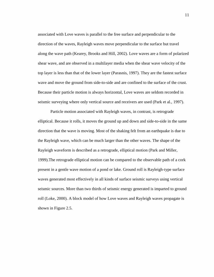
11
associated with Love waves is parallel to the free surface and perpendicular to the
direction of the waves, Rayleigh waves move perpendicular to the surface but travel
along the wave path (Kearey, Brooks and Hill, 2002). Love waves are a form of polarized
shear wave, and are observed in a multilayer media when the shear wave velocity of the
top layer is less than that of the lower layer (Parasnis, 1997). They are the fastest surface
wave and move the ground from side-to-side and are confined to the surface of the crust.
Because their particle motion is always horizontal, Love waves are seldom recorded in
seismic surveying where only vertical source and receivers are used (Park et al., 1997).
Particle motion associated with Rayleigh waves, in contrast, is retrograde
elliptical. Because it rolls, it moves the ground up and down and side-to-side in the same
direction that the wave is moving. Most of the shaking felt from an earthquake is due to
the Rayleigh wave, which can be much larger than the other waves. The shape of the
Rayleigh waveform is described as a retrograde, elliptical motion (Park and Miller,
1999).The retrograde elliptical motion can be compared to the observable path of a cork
present in a gentle wave motion of a pond or lake. Ground roll is Rayleigh-type surface
waves generated most effectively in all kinds of surface seismic surveys using vertical
seismic sources. More than two thirds of seismic energy generated is imparted to ground
roll (Loke, 2000). A block model of how Love waves and Rayleigh waves propagate is
shown in Figure 2.5.

12
Figure 2.5: Block models of mode of propagation for Love waves and Rayleigh
waves (http://geohazardsearthquake.blogspot.com)
Rayleigh waves are used for MASW, ReMi and SASW surveying. Therefore,
herein the focus is on Rayleigh wave velocity.
2.2.2 Rayleigh Waves Velocity. Rayleigh waves are dispersive in nature
(different frequencies travel with different phase velocities). The highest useable
Rayleigh wave frequency (geotechnical purposes) recorded involves particle motion
within the shallowest depth range (~1 wavelength; typically upper few feet) and travels
with a velocity that is mostly a function of the average shear wave velocity within that
depth range. Intermediate frequencies for Rayleigh waves involve particle motions to
intermediate depths (to ~ 1 wavelength) and travel with velocities that are a function of
the average shear wave velocity over those intermediate depth ranges. Also the lowest
useable frequency recorded involves particle motion to greatest depth (1 wavelength) and
travels with a velocity that is a function of the shear wave velocity over that depth range.
Rayleigh wave velocities are generally assumed to be about 90% of the corresponding
shear wave velocities; hence Rayleigh wave phase velocity vs. frequency data can be
transformed into depth vs. shear wave velocity data.

13
In uniform medium, Raleigh wave phase velocities are constant, and can be
determined using the formula:
VR6 - 8β
2VR
4 + (24 - 16β
2 /α
2) β
4VR
2 + 16(β
2 /α
2 – 1) β
6 = 0 (2.6)
VR is Rayleigh wave velocity, β is shear-wave velocity, α is compression-wave velocity
(Kearey, Brooks and Hill, 2002).
Although the Rayleigh wave phase velocity is a function of both compressional () and
shear wave (β) velocities, it is much more sensitive to variations in β than variations in .
Hence, for computational purposes and when dealing with Rayleigh waves propagating
through soil and rock, a value of Poisson’s Ratio is often assumed such that VR is
approximately equal to 0.9 β (Equation 2.7).
VR ~ 0.9 β (2.7)
In non-uniform medium (like typical soils and rock), α and β vary with depth.
Hence, Rayleigh wave phase velocities vary with frequency (wavelength and depth extent
of particle motion). If we can determine how VR varies with frequency, we can determine
how VR varies with depth. If we assume that VR and β are directly related (VR ~ 0.9 β),
we can also determine how β varies with depth.
2.2.3 Relationship between Shear Waves and Soil/Rock Conditions. The shear
wave velocity of a material is very important when predicting the impact earthquake
seismic waves will have on the material as it pass through it (Wood, 2009). By knowing
the S-wave velocity of a material the shear modulus can be determined using the
relationship:
μ=ρVs2 (2.8)

14
Where μ = shear modulus, p = mass density, and Vs = shear wave velocity. The
shear modulus of a material describes how it will react (in terms of stress-strain behavior)
in response to strong ground motion. Hence, shear modulus helps in predicting the
vulnerability of a material to an impending earthquake. The equation above helps to
calculate small strain shear modulus of a material (μmax), when seismic surface wave
methods are used to develop sub-surface Vs profiles at a site. This is due to the small
levels of strain induced in the materials during testing. The sub-surface shear modulus
profile of a site is used to predict ground motion amplification of earthquake waves along
with the possible liquefaction potential of a site (Wood, 2009). Because knowledge of
shear wave velocity can provide critical information about how a material will respond to
different types of loads (static and dynamic), many methods have been developed to
measure this property.
Downhole and crosshole techniques were the earliest methods used to measure in-
situ shear wave velocity profiles (Wood, 2009). These two techniques involve drilling(s)
to the actual depth needed for testing and they directly measure the Vs by determining the
time it takes for shear waves to travel from a known source position (either at the ground
surface or in a borehole) to a known receiver position (in a borehole). The downhole
method involves drilling of one borehole and placing the source at the ground (mostly a
sledge hammer striking a metal plate), while the crosshole method involves drilling more
than one borehole, then placing a source in one borehole and a receiver(s) in the other
hole(s) (Wood, 2009). In this method, the waves propagate between the boreholes and the
source and receivers are both moved to different depths. These methods directly measure
the in-situ shear wave velocity and are therefore considered the most accurate methods

15
for measuring shear-wave velocity (Vs). Although downhole and crosshole methods
provide the most accurate Vs of a sub-surface, they are limited by large cost of drilling
boreholes and are being replaced by surface wave methods which are faster, cost
effective and better alternatives to estimating sub-surface shear wave velocity (Vs)
profiles. The earliest surface wave’s method used was the steady state Rayleigh waves
method followed by Spectral Analysis of Surface Waves method (SASW) (Park et al.,
2000). The steady state Rayleigh waves method uses a mechanical vibrator to produce a
vertical sinusoidal signal that is measured using a single receiver while SASW uses only
two receivers to record ground roll that is usually generated by impact source like a
sledge hammer. Both methods are time and labor intensive due to necessity of repeated
tests with different field configurations, therefore, Multichannel Analysis of Surface
Waves (MASW) method was introduced to mitigate the impending problems of SASW
and Steady State method. For the purpose of this research, the focus is on the
Multichannel Analysis of Surface Waves (MASW) method.
2.3 MULTICHANNEL ANALYSIS OF SURFACE WAVES METHOD
In a layered medium in which seismic velocity changes with depth, both types of
the surface waves have dispersion property that is indicative of elastic moduli of near-
surface earth materials: different wavelength has different penetration depth and
propagates with different velocity. Short wavelength has shallow penetration and longer
one has deeper penetration. The propagation velocity for each wavelength, called phase
velocity (Bath, 1973), depends primarily on the shear (S)-wave velocity (VS) of the
medium over the penetration depth and is influenced only slightly by the compressional

16
(P)-wave velocity, density (ρ), and Poisson's ratio (σ). Therefore, the surface-wave
velocity is a good indicator of shear (S)-wave velocity (VS). It is normally assumed the
phase velocity of ground roll is about 92 percent of VS (Stokoe et al., 1994), and the ratio
changes between 0.88 and 0.95 for the entire range of Poisson's ratio (0. - 0.5) (Ewing et
al., 1957).
Theoretical values for the phase velocities of different wavelengths can be found
by solving the above elastic wave Equation 2.6 with boundary conditions set by the
layered model (Loke, 2000).
Therefore, by analyzing the dispersion feature of ground roll represented in
recorded seismic data, the near-surface S-wave velocity (Vs) profiles can be constructed
and the corresponding shear moduli (μ) are calculated from the relation between the two
parameters:
(2.9)
ρ represents density of material. Change of density with depth is usually small in
comparison to the change in μ and is normally ignored or guessed. With known (or
guessed) Poisson's ratio, one can also obtain P-wave velocity (VP) profile from VS
profile. The entire procedure of generating VS profile consists of three steps: acquiring
ground roll data in the field, processing the data to determine dispersion curve (a plot of
frequency vs. phase velocity), and back calculation of the VS for different depths. The
wavefields of horizontally traveling ground roll are recorded by receivers (geophones)
laid at the surface with certain spacing dx. Recorded wavefields are then analyzed at

17
different frequencies (f) for the phase velocities (Cf) based upon the difference (Δt f) in
the arrival times of ground roll at two receivers as
(2.10)
This analysis produces a set of data ( f vs. Cf), the dispersion data, that are in turn
passed into next step of analysis, the inversion process. The inversion process back
calculates S-wave velocity (VS) profile from the measured dispersion data. Two different
approaches are possible for inversion: forward modeling and least-squares algorithm. The
forward modeling involves assuming a VS profile, and then comparing the theoretical
dispersion curve with the empirical (Stokoe et al., 1994). The assumed profile is modified
until the two curves match closely. The least-squares algorithm seeks the VS profile
whose dispersion curve matches best with the empirical curve in least-squares sense
(Nazarian, 1984; Sanchez-Salinero et al., 1987; Rix and Leipski, 1991). It is an
automated, but computationally intensive method.
2.3.1 Overview. MASW technique was first reported in late 1990s and was
developed by Kansas Geological Survey as an improvement to SASW method (Park et al.
1998, 1999, 2001). It makes use of more than two receivers (array of 12 to 48) deployed
in a linear pattern at equal spacing attached to a single recording system to detect the
higher modes present in the surface waves (Amit Goel1and Animesh Das, 2008). The
multiple receiver spread allows for data acquisition over a larger area, improves modal
separation and provides a means of efficient and continuous data acquisition (Park et al.,
2000). The basic field procedures and acquisition parameters are generally the same as
those used in conventional common midpoint body-wave reflection surveys. Because of

18
these commonalities, the MASW method can be applied to reflection or refraction data if
low frequency receivers are used and no analog low-cut filter is applied during data
acquisition (Park et al., 2001).A typical MASW field setup is shown in Figure 2.6.
Three types of MASW method have been developed at Kansas Geological Survey
Agency (KGS) : multi-channel analysis of surface waves using Vibroseis (MASWV),
multi-channel analysis of surface waves using impulsive source (MASWI) and
multichannel analysis of surface waves using passive source MASWP (Park et al.,
1997a). Each type has difference in type of source used and data processing technique to
generate dispersion curve. MASWV uses a swept source like Vibroseis (Figure 2.7),
MASWI uses an impulsive source like sledge hammer (Figure 2.8) while MASWP uses
ambient noise from a passive source especially moving vehicle along a road side (Figure
2.9). The data processing techniques are a time-domain approach for MASWV (Park et
al., 1999) and a frequency-domain approach for MASWI and MASWP (Park et al.,
1997a). When a combined dispersion curve of an extended frequency range is prepared
from analyses of both passive and active surface waves it increases the maximum depth
of Vs estimation (Park et al., 2001).
For the purpose of this research, the focus is on the Multichannel Analysis of
Surface Waves using an impulsive source.

19
Figure 2.6: Showing typical MASW field setup (Park et al., 1997)
Figure 2.7: Showing typical MASWV field setup (Park et al., 1997)
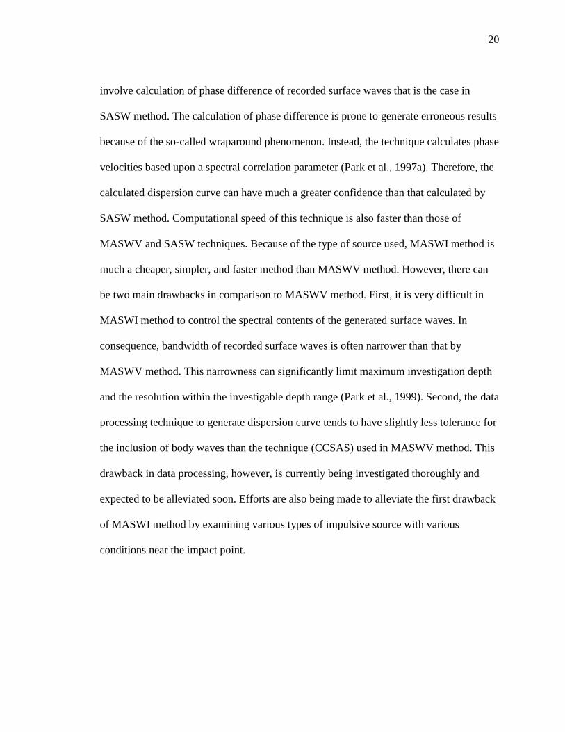
2.3.2 MASW Using Impulsive Source (MASWI). The method of multi-channel
analysis of surface waves using impulsive source (MASWI) is a similar method to
multichannel analysis of surface waves using Vibroseis (MASWV) method. Two main
differences are, however, in type of the source used and the data processing technique to
generate dispersion curve. Instead of a swept source like Vibroseis, an impulsive source
like a sledge hammer is used. The data processing technique is a frequency-domain
technique, instead of a time-domain technique of CCSAS in MASWV method, similar to
the spectral analysis technique used in SASW method. The technique, however, does not
20
involve calculation of phase difference of recorded surface waves that is the case in
SASW method. The calculation of phase difference is prone to generate erroneous results
because of the so-called wraparound phenomenon. Instead, the technique calculates phase
velocities based upon a spectral correlation parameter (Park et al., 1997a). Therefore, the
calculated dispersion curve can have much a greater confidence than that calculated by
SASW method. Computational speed of this technique is also faster than those of
MASWV and SASW techniques. Because of the type of source used, MASWI method is
much a cheaper, simpler, and faster method than MASWV method. However, there can
be two main drawbacks in comparison to MASWV method. First, it is very difficult in
MASWI method to control the spectral contents of the generated surface waves. In
consequence, bandwidth of recorded surface waves is often narrower than that by
MASWV method. This narrowness can significantly limit maximum investigation depth
and the resolution within the investigable depth range (Park et al., 1999). Second, the data
processing technique to generate dispersion curve tends to have slightly less tolerance for
the inclusion of body waves than the technique (CCSAS) used in MASWV method. This
drawback in data processing, however, is currently being investigated thoroughly and
expected to be alleviated soon. Efforts are also being made to alleviate the first drawback
of MASWI method by examining various types of impulsive source with various
conditions near the impact point.

21
Figure 2.8: Showing typical MASWI field setup (Park et al., 1997)
Figure 2.9: Showing different array configurations for the MASWP (Park et al.,
1997)
2.4 MASW EQUIPMENT
Equipment required to conduct MASW analyses is comprised of five elements: a
seismic source, a triggering device, receivers, transmitting cables and a multichannel
seismograph.
2.4.1 Seismic Source. A seismic source is used to transfer energy to the ground
for the purposes of inducing seismic wave activity. In practice, a source can be an impact
force applied to the ground by a hammer or falling weight, a small scale explosion

22
detonated within the subsurface, or a mechanical vibratory device (Loke, 2000). A
sledgehammer with either a metallic or stiff rubber strike plate provides an inexpensive
and easily transferrable impact source. However, for surveys requiring a higher degree of
energy transfer, a falling weight may also be used to provide an impact source. Explosive
sources such as downhole gun fire or explosives used during quarry operations are less
frequently used due to expense and safety; however, given the application explosive
sources can provide strong surface wave signals for data acquisition (Loke, 2000). Swept
frequency sources provide a signal with a constant frequency. The selection of a seismic
source should be based on the signal requirements of the survey, cost and relative safety
(Kearey, Brooks and Hill 2002). For most shallow surface evaluations, the use of a
sledgehammer and striker plate provides an adequate seismic signal (Park et al., 2009).
2.4.2 Trigger Mechanism. The triggering mechanism is needed to signal the
seismography and synchronize the time with the arrival of the transmitted surface wave
(Loke, 2000). For impact sources, such as a sledgehammer or drop weight, an open
circuit mechanism is attached to the source, which closes at the moment of contact. An
example of a simple triggering system attached to a sledgehammer is provided in Figure
2.10. In an ideal situation, the trigger would provide an instantaneous signal marking the
initiation of the survey (Milson, 1996). However, in practice it is understood that there is
a small lag in between the actual strike event and the time for which the signal is
transmitted to the seismography that the strike event has occurred. Lag time can be
predetermined for a particular trigger instrument and subsequently programmed into
seismograph use during data acquisition (Geometrics Incorporated, 2003).

23
Figure 2.10: Example of Sledgehammer Triggering Device (Milson, 1996)
2.4.3 Geophones. Receivers, or geophones, are electromechanical transducers
that convert ground motion into an electrical analog signal (Pelton, 2005). The current, or
signal, produced is proportional to the velocity of the oscillating coil system through the
internal magnetic core (Milson, 1996). The movement of the internal core is relative to
the ground movement below the geophone, as the seismic wave(s) pass the respective
receiver (Kearey, Brooks and Hill, 2002). Figure 2.11 provides an example of the
configuration of a spike-coupled geophone. Geophones with single, vertical axis of
vibration are commonly used to measure incoming signals immediately below the
receiver. Other geophones with horizontal or multiple axis capabilities are available, but
are not commonly used for MASW applications (United States Corps of Engineers,
1995). For the purpose of this research, 4.5 Hz geophones with steel spikes were used.
The geophone must be well coupled with the earth. Steel spikes are typically used for
coupling geophones; however, in some applications the use of steel plates has proven to
be comparable to the use of steel spikes. Advancements in receiver deployment have led

24
to towable instruments such as the land streamer, which uses a weighted geophones and
cable system equipped with robust steel plates for coupling. For MASW applications,
lower frequency receivers (e.g. 2 Hz, 4.5 Hz) provide better performance due to the
ability to capture deeper transmitted signals (Park et al., 2009).
Figure 2.11: Example of spike-coupled Geophone (Milson, 1996)
2.4.4 Geophone Cable. Analog electrical impulses are transmitted from the
individual geophones to the seismograph through a cable system. The cable is metallic
and transmits the signal with little resistance; however, due to the potential for “cross-
talk” between the geophone cable and the trigger switch, consideration should be given
during data acquisition to maintaining a sufficient distance between the two elements
(Milson, 1996).

25
2.4.5 Seismograph. Seismographs are used to record and interpret the transmitted
signal from the geophone into a discernable trace or shot record (Milson, 1996).
Seismographs can range in complexity from simple timing instruments to
microcomputers capable of digitizing, storing and displaying received shot records.
Multichannel seismographs allow for the acquisition of multiple independent readings.
Systems with 24 channels are common in shallow surface investigations; however,
deeper applications may utilize a greater number of channels (Milson, 1996). RAS-24
Seistronix seismograph was used for this research because it was available and has all the
required specifications.
2.5 MASW FIELD SURVEY SETUP
Field setup for data acquisition is similar to that of the common midpoint
reflection survey. Figure 2.13 is an exhibit showing the typical linear layout and the
progressive movement of a survey during a profiling application (Park et al., 2009).While
Figure 2.12 is array configurations of MASW survey.
Consideration should be given to the geophone interval spacing, as an increased
length will improve depth and modal separation but will also increase the amount of
spatial averaging of data during processing (Park, 2005).

26
Figure 2.12: Instrumentation of MASW Tomography Survey (Park et al., 2004)
2.5.1 Overviews of MASW Data Acquisition. The survey begins at the instance
that the seismic source initiates the wave signal. The triggering system notifies that
seismograph when data recording should begin. In order to acquire strong surface signals,
it is recommended that sampling intervals range from 0.5 to 1.0 millisecond and
recordings times range from 500 milliseconds to 1,000 milliseconds. A variation in
required recording times and sampling intervals is generally a function of subsurface
conditions (e.g. slower velocities from softer soil conditions). As demonstrated in Figure
2.13, the shot record is created from the trace signals returned to the seismography by the
geophones. The individual geophone records are known as traces. After recording the
first shot record, the line of geophones is advanced a predetermined interval down the
survey line, and preparations are made to collect the next shot (Park et al., 2009). The
length of the geophone array shift dictates the resolution of the tomography profile. Shot

27
Interval distances beyond the spread length increased the required averaging of soil
properties and introduced smearing to the imagery. Due to MASW testing requiring a
constant receiver spacing, it is very important that the spacing be small enough to prevent
far offset effects. The spacing also controls the minimum wavelength that can be
measured by the array due to spatial aliasing. Spatial aliasing occurs when receiver pairs
measure wavelengths that are less than 2 times the spacing between the receivers. Park et
al. (2001) advises that receivers should normally be spaced at 1 meter intervals with a
maximum source offset of 100 meters. For the purpose of this research, an active source
(20-lbs sledge hammer) was used. The geophone spacings used were 1-ft, 2.5-ft, 5-ft, 7.5-
ft and 10-ft, while offset distances chosen were 0-ft, 10-ft, 20-ft, 30-ft, 40-ft and 50-ft.
Figure 2.13: Progression of MASW Tomography Survey (Park et al., 2004)
2.5.2 Overviews of Data Processing. Three steps must be performed in order to
convert shot record data to estimations of shear wave velocity: initial processing of shot

28
record for surface wave phase velocity and frequency for development of dispersion
curves, identification of fundamental mode, and inversion of the fundamental mode
curvature into a representative shear wave profile (Figure 2.14).
Figure 2.14 Processing Steps to Estimate Shear Wave Velocity (Park et al., 2004)
After field surveying is complete, each collected shot record is processed,
highlighting the present surface wave signatures. The raw shot record may contain other
wave forms, such as refracted waves, body waves, and sources of cultural noise.
However, one of the main advantages of the MASW seismic technique is that the
strength of the utilized surface wave is much greater than other wave forms; therefore
surface waves are more discernable in the presence of noise. In a record presenting good
signal to noise (S/N) ratio, the signal strength of the surface wave should be evident by
the linear sloping features of the dispersive wave forms. Surface waves, on an active shot
record, are often identified noted by the smooth sloping behavior as the wave travels
down the geophone array (Park et al., 2009). This linear slope represents the phase
velocity of the particular surface wave, and can be used to transform the shot record data

29
into a dispersion curve relating phase velocity to wave frequency (Park et al., 2000).
Developed analysis software, such as Surfeis, can process shot records and extract
dispersion curves through the initial processing sequences (Park et al., 2009).Before the
phase velocity and frequency information can be inverted, the fundamental mode of the
surface wave must be identified. The dispersion curve is produced by processing the shot
record data using specialized algorithms (e.g. frequency-wavenumber spectrum,
slowness-frequency transformation, KGS wavefield transformation). The resulting
dispersion curve plot relates phase velocity within the frequency domain. As shown in
Figure 2.14, the generated image contains the fundamental mode, as well as artifacts from
higher modes and other wave forms. The fundamental mode of the dispersion curve is
identified by the strongest energy signature in the dispersion curve. At this time,
automated selection of dispersion curves is not available, therefore it is still necessary to
manual identify the curvature of the fundamental mode. Higher mode contamination of
the shot record can hinder the selection of the fundamental mode, and introduce error into
the MASW analysis (Park et al., 2009).
The inversion process for MASW is similar the inversion process used for ERT
analysis. A forward modeling algorithm is used to generate an earth model with layers of
varying shear wave velocity. The generated model is an attempt to match an actual
layered earth model, for which the exhibited shear wave condition could exist. A root
mean square analysis is used to evaluate the fitting of the derived curve with the actual
curve extracted from the field data. Before the iterative process is ended, the derived
model must either satisfy the error tolerance or the number of iterations performed must
exceed number of iterations allowed for convergence. The inverted section represents an
30
estimate of shear wave velocity with respect to depth (Park et al., 2009). The inverted
section represents an averaged condition below the given geophone spread. To assign a
spatial coordinate to the reading, it is assumed that the layered earth model is
representative of subsurface conditions below the mid span, or mid station location of the
geophone array. Downhole measurements have been used to test the validity of the mid
station assumption. Results from testing have indicated that the use of MASW, with the
mid station assumption, provides a reasonable estimation of profiled shear wave
properties when compared against downhole measurements of the same area (Park et al.,
2000).
The inversion process for MASW is performed prior to the development the
tomography profile. Since a unique shear wave velocity profile is generated for each shot
along the survey line, the individual profiles can be interpolated to create a single two-
dimensional image representing lateral and vertical variations in shear wave velocity. No
additional inversion is required. Interpolation can be performed using an equal weighting
or variant weighting system (Park et al., 2009).
31
3 OVERVIEWS OF ELECTRICAL RESISTIVITY TOMOGRAPHY
METHOD
3.1 INTRODUCTION
Just as soil and rock materials have both physical and chemical properties;
subsurface materials also present unique electrical characteristics. Surface electrical
resistivity surveying is based on the principle that the distribution of electrical potential in
the ground around a current-carrying electrode depends on the electrical resistivities and
distribution of the surrounding soils and rocks. Mineral grains comprised of soils and
rocks are essentially nonconductive, except in some exotic materials such as metallic
ores, so the resistivity of soils and rocks is governed primarily by the amount of pore
water, its resistivity, and the arrangement of the pores. To the extent that differences of
lithology are accompanied by differences of resistivity, resistivity surveys can be useful
in detecting bodies of anomalous materials or in estimating the depths of bedrock
surfaces. In coarse, granular soils, the groundwater surface is generally marked by an
abrupt change in water saturation and thus, by a change of resistivity. In fine-grained
soils, however, there may be no such resistivity change coinciding with a piezometric
surface.
Generally, since the resistivity of a soil or rock is controlled primarily by the pore
water conditions, there are wide ranges in resistivity for any particular soil or rock type,
and resistivity values cannot be directly interpreted in terms of soil type or lithology.
Commonly, however, zones of distinctive resistivity can be associated with specific soil
or rock units on the basis of local field or drill hole information, and resistivity surveys

32
can be used profitably to extend field investigations into areas with very limited or
nonexistent data.
Practitioners in geologic, environmental and engineering fields utilize electrical
resistivity soundings and tomography to map fluctuations in conductive behavior
(Milson, 1996). Recent advancements in equipment and software have automated both
data acquisition and processing, making electrical resistivity one of the most versatile
methods for both the practicing geophysicist and engineering professionals (Steeples,
2001).
3.2 BASIC THEORY
The fundamental principle behind collection and interpretation of electrical
resistivity measurements originates in the electrical physical theory of Ohm’s Law.
Ohm’s Law, Equation 2.10, states that the product of the electrical current, I, through a
conductor and the resistance of the conductor, R, for which the current passes, is
equivalent to the potential difference, V, across the conductor.
V = IR 2.10
This relationship is best represented by envisioning current passing through a thin
wire. The expounded application of the Ohm’s Law has made this relationship a capstone
concept in the study of electrical theory (Gibson and George, 2003). Units for electrical
potential, current, and resistance are volts, amperes, and ohms, respectively.
As suggested, the conductor element can tangibly be described as a wire element.
The resistance of the wire is related to both the geometric shape and material attributes of
the wire (Milson, 1996). The geometry of the wire is typically cylindrical, therefore

33
possessing a length and cross-sectional area, and is made of a conductive material. The
total resistance of the wire element, R, is the product of the material resistivity, ρ, and the
ratio of the wire length and cross-sectional area.
R = ρ (L/A) 2.11
Considering the physical relationship between the geometry of the conductor and
the material property, Equation 2.11 can be manipulated to determine the material
resistivity of the conductor element.
ρ = R (L/A) 2.12
This form states that the units for resistivity are dependent on the volume of space
for which the current travels. Typical units for resistivity, ρ, include ohm-meter and ohm-
centimeter (Gibson and George, 2003).
In similar context, the measurement of potential difference can be related to the
dissipation of electrical current within an infinite, homogenous half-space. In this
scenario, the application of an electrical current is travels in radial fashion out from the
point of origin. During the current application, the resistance at any location away from
the point of origin within the homogeneous mass can be found by determining the radius
from the point of origin and the surface area of the respective hemispherical equipotential
surface. Relating this model to the original wire example, Equation 2.11 can be rewritten
using the radius, r, as the distance for which the current travels and the surface area of the
resulting equipotential surface, 2πr2. Equation 2.13 describes the system resistance at any
point away from the point source, within the homogeneous mass.
R = ρ(r/2πr2) = (ρ/2πr) 2.13

34
Using the resistance term from the aforementioned homogeneous earth model,
Equation 2.14 relates the resistance of the earthen model to Ohm’s Law.
2.14
U = potential, in V, ρ = resistivity of the medium, r = distance from the
electrode
Likewise, the potential difference between any two points within the
homogeneous mass would be the difference between the two equipotential surfaces, as
expressed in Equation 2.15 (Gibson and George, 2003).
2.15
Where rA and rB = distances from the point to electrodes A and B
Therefore, ρ = (2πՍ/I) [1/ [(1/ra)-(1/rb)] 2.16
Equation 2.16 relates the applied current, I, and measured potential difference, V,
to a constant value which accounts for spatial considerations, or the way in which the
reading was acquired. This model and concept of equipotential surfaces and means of
measuring potential differences between various surfaces is fundamental to the
interpretation of collected field data (Gibson and George, 2003).
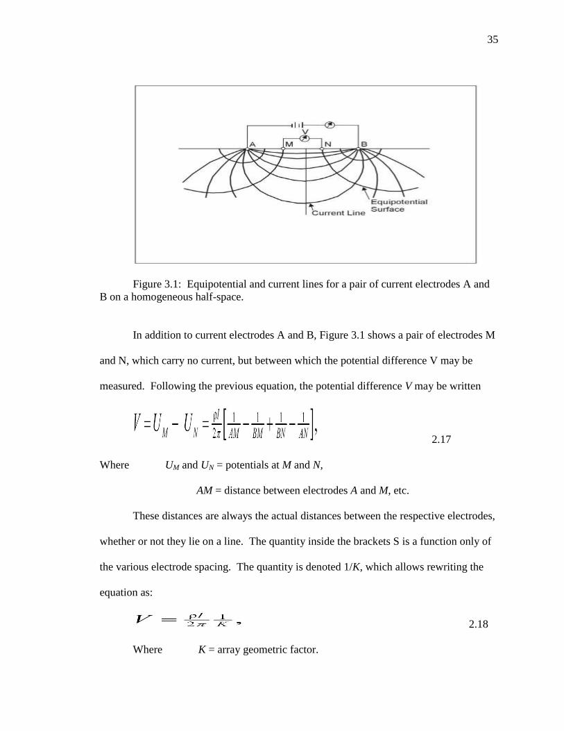
Figure 3.1 illustrates the electric field around the two electrodes in terms of
equipotential and current lines. The equipotential represent imagery shells, or bowls,
surrounding the current electrodes, and on any one of which the electrical potential is
everywhere equal. The current lines represent a sampling of the infinitely many paths
followed by the current, paths that are defined by the condition that they must be
everywhere normal to the equipotential surfaces.
35
Figure 3.1: Equipotential and current lines for a pair of current electrodes A and
B on a homogeneous half-space.
In addition to current electrodes A and B, Figure 3.1 shows a pair of electrodes M
and N, which carry no current, but between which the potential difference V may be
measured. Following the previous equation, the potential difference V may be written
2.17
Where UM and UN = potentials at M and N,
AM = distance between electrodes A and M, etc.
These distances are always the actual distances between the respective electrodes,
whether or not they lie on a line. The quantity inside the brackets S is a function only of
the various electrode spacing. The quantity is denoted 1/K, which allows rewriting the
equation as:
2.18
Where K = array geometric factor.
36
Equation 2.18 can be solved for ρ to obtain:
2.19
The resistivity of the medium can be found from measured values of V, I, and K,
the geometric factor. K is a function only of the geometry of the electrode arrangement.
In a homogenous media, the measured resistivity will be equivalent to the true
value of resistivity at a given location with the media. However, the occurrence of a
homogenous condition is rare, if not non-existent in practice. In order to account for the
inherent heterogeneity of the earth, a collected reading is considered an apparent
resistivity measurement. Apparent resistivity is the resistivity of a theoretical,
homogeneous half-space which complements the measured current and potential
difference for a particular measurement scheme (United States Corps of Engineers,
2001). Essentially, the apparent resistivity value is an average reading of the energized
soil mass engaged during the measurement. Wherever these measurements are made over
a real heterogeneous earth, as distinguished from the fictitious homogeneous half-space,
the symbol ρ is replaced by ρa for apparent resistivity. The resistivity surveying problem
is reduced to its essence, the use of apparent resistivity values from field observations at
various locations and with various electrode configurations to estimate the true
resistivities of the several earth materials present at a site and to locate their boundaries
spatially below the surface of the site. An electrode array with constant spacing is used to
investigate lateral changes in apparent resistivity reflecting lateral geologic variability or
localized anomalous features. To investigate changes in resistivity with depth, the size of
the electrode array is varied. The apparent resistivity is affected by material at
increasingly greater depths (hence larger volume) as the electrode spacing is increased.

37
Because of this effect, a plot of apparent resistivity against electrode spacing can be used
to indicate vertical variations in resistivity.
The geometric coefficient, K, varies with array types. The spacing and layout of
current and potential electrodes impacts the induced equipotential fields generated within
the earthen mass (refer to Figure 3.2 for Wenner, Schlumberger, and Dipole-Dipole
arrays). Referencing Equation 2.16, the geometric factor for a general four probe system
can be derived (Gibson and George, 2003).
3.3 ARRAYS
Theoretically, soil resistivity could be measured by using a single current source
and receiver element. In practice, this is not feasible due to the contact resistance between
the earth and the electrode pair. To overcome this phenomenon, four electrodes are used
for measurement; two electrodes providing current to the earth and two electrodes for
measuring potential difference within the earth (Milson, 1996). Current electrodes are
identified as C1 and C2 (or A and B), and potential electrodes are identified as P1 and P2
or (M and N) (Loke, 2000).
The types of electrode arrays that are most commonly used are Schlumberger,
Wenner, and dipole-dipole. There are other electrode configurations that are used
experimentally or for non-geotechnical problems or are not in wide popularity today.
Some of these include the Lee, half-Schlumberger, polar dipole, dipole -dipole, and
gradient arrays. In any case, the geometric factor for any four-electrode system can be
found from Equation 2.17 and can be developed for more complicated systems by using
the rule illustrated by Equation 2.15 (United States Environmental Protection Agency,

38
2011). It can also be seen from Equation 2.19 that the current and potential electrodes
can be interchanged without affecting the results; this property is called reciprocity
(Milson, 1996). For the purpose of this research, the discussion will focus on the dipole-
dipole array which was used for this research.
Figure 3.2: Electrode array configurations for resistivity measurements (United
States Environmental Protection Agency, 2011).
Unlike the Wenner and Schlumberger arrays, the configuration of the dipole-
dipole array does not place the potential electrode pair inside the current electrode pair.
Current and potential electrode pairs have common interior spacing, and separated by a
distance ten times the interior spacing of the electrode pair. The dipole-dipole array is
commonly used for performing tomography surveying due to the array’s ability to resolve

39
lateral variations. In comparison to the Wenner and Schlumberger arrays, the dipole-
dipole array has a weaker signal and is more susceptible to the effects of ambient or
cultural noise (United States Environmental Protection Agency, 2011).
If the separation between both pairs of electrodes is the same a, and the separation
between the centers of the dipoles is restricted to a (n+1), the apparent resistivity is given
by:
2.20
3.4 RELATIONSHIP BETWEEN RESISTIVITY AND SOIL/ROCK CONDITION
Electrical resistivity testing represents a broad category of geophysical testing,
including measurements of spontaneous potential, induced polarization, and apparent
resistivity measurements (Loke, 2000). Spontaneous potential (SP) is a method designed
to measure variations in conductive behavior occurring without introducing an auxiliary
current source. Induced polarization is a method measuring the time-rate decay of
polarizing effects resulting from the induced current (Loke, 2000). This method is
effective in delineating contaminant plumes and mineral ore bodies, which often present
with unique decay signatures when compared against other ambient conditions (Gibson
and George, 2003). Among the electrical resistivity testing methods, apparent resistivity
measurement is the most utilized method for engineering applications (Loke, 2000).
Apparent resistivity can be analyzed in either by vertical sounding, two dimensional
profile, three dimensional models, or time variant analysis (Gibson and George, 2003).
40
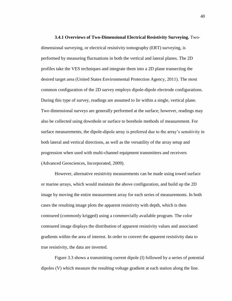
3.4.1 Overviews of Two-Dimensional Electrical Resistivity Surveying. Two-
dimensional surveying, or electrical resistivity tomography (ERT) surveying, is
performed by measuring fluctuations in both the vertical and lateral planes. The 2D
profiles take the VES techniques and integrate them into a 2D plane transecting the
desired target area (United States Environmental Protection Agency, 2011). The most
common configuration of the 2D survey employs dipole-dipole electrode configurations.
During this type of survey, readings are assumed to lie within a single, vertical plane.
Two dimensional surveys are generally performed at the surface; however, readings may
also be collected using downhole or surface to borehole methods of measurement. For
surface measurements, the dipole-dipole array is preferred due to the array’s sensitivity in
both lateral and vertical directions, as well as the versatility of the array setup and
progression when used with multi-channel equipment transmitters and receivers
(Advanced Geosciences, Incorporated, 2009).
However, alternative resistivity measurements can be made using towed surface
or marine arrays, which would maintain the above configuration, and build up the 2D
image by moving the entire measurement array for each series of measurements. In both
cases the resulting image plots the apparent resistivity with depth, which is then
contoured (commonly krigged) using a commercially available program. The color
contoured image displays the distribution of apparent resistivity values and associated
gradients within the area of interest. In order to convert the apparent resistivity data to
true resistivity, the data are inverted.
Figure 3.3 shows a transmitting current dipole (I) followed by a series of potential
dipoles (V) which measure the resulting voltage gradient at each station along the line.
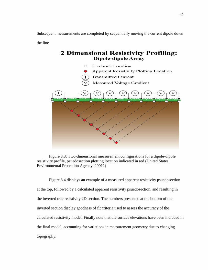
41
Subsequent measurements are completed by sequentially moving the current dipole down
the line
Figure 3.3: Two-dimensional measurement configurations for a dipole-dipole
resistivity profile, psuedosection plotting location indicated in red (United States
Environmental Protection Agency, 20011)
Figure 3.4 displays an example of a measured apparent resistivity psuedosection
at the top, followed by a calculated apparent resistivity psuedosection, and resulting in
the inverted true resistivity 2D section. The numbers presented at the bottom of the
inverted section display goodness of fit criteria used to assess the accuracy of the
calculated resistivity model. Finally note that the surface elevations have been included in
the final model, accounting for variations in measurement geometry due to changing
topography.

42
Figure 3.4: Examples of measured apparent resistivity, calculated apparent
resistivity, and inverted resistivity (Advanced Geosciences, Incorporated, 2009).
3.4.2 Three-Dimensional Electrical Resistivity Surveying (3-D). During a
three-dimensional survey, measurements of potential difference are made in all three
spatial coordinate planes. This allows for the analysis of a target volume, as opposed to
planar section. Three-dimensional surveys may either be performed along the surface,
using crosshole methods, or using surface to borehole measurements. Analytical software
now allows for the compilation of multiple two-dimensional survey data, into a three-
dimensional representation (Advanced Geosciences Incorporated, 2008). For this
research Voxler software was used to compile multiple 2-D survey data into a 3-D model.

43
3.5 FIELD EQUIPMENT
The basic setup required for field measurements includes a transmitter, receiver,
conductive cables, a set of electrodes and a power source (United States Corps of
Engineers, 1995).
3.5.1 Transmitter/Receiver. The function of the transmitter is to apply and
regulate a known current through the instrumentation, to the earth. To acquire the desired
survey penetration and resolution, it is important that the chosen transmitter is capable of
emitting ample current through the system. Previous instrumentation required manual
current adjustments until applicable readings were made. However, with advancements in
technology, newer transmitters are capable of self-regulating current flow to promote the
best possible signal for data acquisition. In addition, various instruments are now capable
of conveying larger currents, also improving signal strength and resolution. Advanced
Geosciences, Incorporated (AGI) produces three different automated units, with
maximum current outputs ranging from 500 milliamps to 2,000 milliamps. The most
recent development by AGI is a system capable of transmitting a current up to 27 amps
(Advanced Geosciences, Incorporated, 2009).
As the transmitter applies a known current, a receiver is needed to measure the
resulting potential reading. Newer instrument, equipped with digital processing
capabilities, are capable of sending the required current, as well as measuring and
receiving the respective potential difference measurement. The sensitivity of the receiver
should be established prior to initiating a survey to ensure that goals of the survey are met
(Advanced Geosciences Incorporated, 2008). Single channel transmitters/receivers are
only capable of collecting one reading at a time. Although single channel instruments are

44
still in use for VES surveys, two and three dimensional surveys are optimized by multi-
channel systems allowing for the acquisition of multiple readings in a single current
output (Advanced Geosciences Incorporated, 2008).
3.5.2 Cables. Metallic cables are used to convey current from the transmitter and
to return measurements of difference to the receiver. The use of highly conductive
metallic material, such as copper, helps minimize losses during data acquisition.
Depending on the transmitter/receiver system utilized, the cables are either composed of
a single wire strand, or a core housing multiple strands accommodating each of the
available channels. Cables are needed for connecting the transmitter/receiver with the
potential electrodes (Advanced Geosciences Incorporated, 2008).
3.5.3 Current and Potential Electrodes. Electrodes are used by the transmitter
to transfer current to the subgrade, and by the receiver to detect fluctuations in electrical
potential. For general use, steel, copper or bronze stakes are common. For applications
requiring refined measurements, readings taken in noisy environments or areas with high
contact resistance, using electrodes with of ceramic components emitting a metallic
aqueous solution, such as copper sulfate, is a viable alternative (Loke, 2000). Sufficient
bedding of electrodes is required in order to couple the resistivity setup with the earth. As
noted, surface conditions with high contact resistance can be overcome by using ceramic
electrodes with a metallic aqueous solution, or, if using metallic stakes, by placing a
saline solution around the base of the electrode (Advanced Geosciences Incorporated,
2008).
When using a direct current for testing purposes, there is a potential that the
charges on the exterior of the electrode will take on a common charge over the surface of

45
the electrode, effectively polarizing the electrode, if the current is applied in one direction
for an extended period of time. In order to prevent polarization, most modern instruments
routinely reverse signals to reverse potential charge buildups (United States Corps of
Engineers, 1995).
3.5.4 Power Source. The transmitter requires a power source in order to pull a
current for the data acquisition system. Required power sources vary by instrument, and
range from internal rechargeable batteries to external generator power sources. For newer
instruments, due to the low power emission required and short duration of discharge, dry
cell batteries can be used for this application. Dry cell batteries are preferred because the
ability to drain and recharge the battery without damaging the core (Advanced
Geosciences Incorporated, 2008). A wet cell battery was used in this survey because of
its availability and durability
3.6 OVERVIEW OF ERT DATA ACQUISITION
Newer instruments are equipped with multiple channels, which allows for
multiple electrodes to be engaged and measurement to be taken through each channel.
For instance, the SuperSting R8 resistivity meter, produced by Advanced Geosciences,
Incorporated, is equipped with eight channels. Therefore, for each current injection, the
system engages nine electrodes to collect eight different potential difference
measurements (Advanced Geosciences, Incorporated, 2006).
Unlike the single channel transmitter, multiple channel equipment has to receive
instruction on the proper triggering sequence of electrodes. This information can either be
programmed directly into the instrument through manual entry, or indirectly by uploading
46
coded command file (Loke, 2000). The sequencing information considers the array style
and information pertaining to the electrode locations or electrode address during each
measuring sequence. There are no theoretical limits to the depth of penetration. However,
as the electrode spacing increases signal strength decreases. At a certain electrode
separation distance, the signal strength is too low to provide reliable measurements of
potential difference. Practical limits should be instilled considering the signal strength of
the particular array type and equipment capabilities. (Advanced Geosciences
Incorporated, 2008) suggested that when considering depth of penetration for
tomography applications, practitioners can generally assume that the depth of penetration
is approximately 15 to 25 percent of the length of the electrode spread. Survey resolution
is also related to electrode spacing. Current practices suggest that the electrode spacing
not be greater than twice the size of the object or feature to be imaged. The design of the
survey (i.e. Survey run length, electrode spacing, and array type) directly impacts the
depth of penetration and resolution (Advanced Geosciences Incorporated, 2008).
It is not always possible or practical to image a survey line or area in one
deployment of electrodes. To continue a survey after completion of the initial data
collection, electrodes may be configured to collect additional data along a common
survey line or area, using roll-along survey techniques (Loke, 2000). In this research, 5-ft
electrode spacing was used. The metal stakes are made of steel and SuperSting R8 was
used to measure the resistivities.

47
3.7 DATA PROCESSING AND INTERPRETATION
Field measurements must be converted into a visual representation for analysis
purposes. Referring to Equation 2.18, calculation of apparent resistivity requires a
geometric factor. Measurements taken from the field provide readings of induced current
and respective potential difference, so by coordinating field data with respective electrode
coordinates and known array type, the geometric factor can be determined and apparent
resistivity is calculated. In addition, recorded field measurements are assigned a
coordinate location, which correlate to the array type used and electrode spacing at the
time of the potential difference reading. The mapping of apparent resistivity values
creates a profile termed a psuedosection (Milson 1996, Loke 2000, Gibson and George
2003). Pseudosections (Figure 3.5) provide a crude representation of the resistive
environment surveyed, and attempting an interpretation from a psuedosection can be
misleading (Zonge, Wynn and Urquatt, 2005).
Figure 3.5: Example of Developed Psuedosection Model Using a Wenner Array
and 28 Electrodes (Loke, 2000)

48
Although the “true” point measurements is unattainable using surface survey
methods, apparent values can be effectively used to estimate “true” subsurface conditions
(Loke, 2000). Apparent resistivity pseudosections provide the necessary data to complete
an iterative inversion process. The purpose of the inversion is to produce a matching or
representative earth model which would produce a like psuedosection. Iterations continue
until the modeled psuedosection approaches convergence with the measured
psuedosection. Currently there are no means of directly correlating apparent resistivity
measurements to an earthen model (Zonge, Wynn and Urquatt, 2005).
Figure 3.6 provides a generalized flow chart demonstrating the typical processes
required to complete the inversion process. The convergence criterion is usually a
predetermined tolerance for calculated error between the measured and modeled
resistivity. Statistical analysis of data (e.g. root mean square error analysis, L2
normalization) is used to gauge the refinement of the final model. Smoothing algorithms
are also used to eliminate or lessening the impact of data points not conforming to the
trends of the model (Advanced Geosciences, Incorporated 2009, Zonge et al., 2005). The
inversion process is best performed using numerical analysis software due to the quantity
of data involved and iterative processes. Software packages such as RES2DINV,
RES3DINV and EarthImager 1D, 2D, and 3D are examples of products available for
inversion processing and inversion (Advanced Geosciences Incorporated, 2008, 2009).

49
Figure 3.6: Flow Chart of Resistivity Inversion Processing (Society of
Exploration Geophysicist of Japan, 2004)
In survey situations with significant variations in terrain, estimated resistivity
measurements may mask subsurface features if site topography is not considered (Zonge
et al., 2005).
Therefore, site conditions should be considered; excessive dip of subsurface strata
along the survey line (more than about 10 percent), unfavorable topography, or known
high lateral variability in soil or rock properties may be reasons to reject field data as
unsuitable for interpretation in terms of simple vertical variation of resistivity. But the
effects of topographic changes on generated tomography images can be resolved during
the inversion process (Advanced Geosciences Incorporated, 2008).

50
4 RESEARCH METHODS
4.1 OVERVIEW
This section presents the methodology behind the site selection, data collection
setup, and data collection procedures used in this acquisition and processing. The focus
will be on the MASW and Electrical Resistivity Tomography methods, and will provide a
guide to those collecting these types of data in the similar environment.
4.2 SITE LOCATION
A single site was chosen for this research. It is located in Newburg, Missouri
Area. This site was chosen due to its proximity to the university, and it is flat (no
complex topography) and has easy accessibility. Newburg map in Figure 4.1 shows that
study area is located close to the Corn Creek Road within the Mark Twain National
Forest area in south west of Newburg.
Figure 4.1: Newburg map showing the study area located within Mark Twain
National Forest (Courtesy of Google Earth).

51
The Corn Creek Road is located at the southwest corner of high way 63 and
southeast of Interstate 44 (Figure 4.2.)
Figure 4.2: Showing the location of Corn Creek Road (courtesy of Google Earth)
The exact location of the site is given by coordinates: 37°48'31.00" N and 91°52
'05.70" W and elevation of 955-ft above the sea level.
The site geology consists of alluvium and residuum deposits which depicts an old
river channel. Alluvium and Surficial geology map of the area shows that the site is
within a flood plain (Figure 4.3).

52
(a) Broader view
(b) Enlarged view
Figure 4.3: Alluvium and Surficial geology map of the Newburg area (courtesy of Google
Earth)

53
The alluvium deposits are predominately loose soil (regolith) while the K-
residuum is comprised of Cherty sandy clay and sandy clay, reddish brown to brown, 1-
10-ft. thick, developed as residuum from sandy dolomite, dolomite, sandstone and chert.
Residuum is stony clay and clayey sand containing relict layers of sandstone and chert, 5-
10-ft. thick, generally covered by coarse cherty colluvium on hillslopes and a thin loess
mantle on uplands (http://dnr.mo.gov/GIS/GEOLOGY.SURFICIAL.XML). Figure 4.4
show the bedrock, geologic map and geologic unit of the study area.
Figure 4.4: Bedrock Geologic map of the study area (Courtesy of Google Earth).
The bedrock is an early Ordovician deposit known as Gasconade Formation
which is dominated by dolomite and a little intercalation of chert overlain by the
Roubidoux Formation containing mostly dolomite, sandstone, banded chert, shale and
some siliceous oolites , respectively ,according to their order of dominance. Roubidoux
54
Formation was severely eroded during the transgression stage of the glaciation age, and
few thickness of alluvium was deposited after the transgression age. The K- residuum
could be residuals from weathered bedrock.
Multichannel Analysis of surface waves (MASW) were acquired along two lines
with five array configurations. The first configuration consisted of 24 geophones (4.5 Hz
natural frequency) placed at a uniform spacing of 1-ft. with a total array length of 23-ft.
while the offset distances for the geophones were placed at different intervals in the order
of 0-ft to 50-ft. For the second array configuration, the 24 geophones were spaced 2.5-ft
apart uniformly while maintaining the same offset distances at interval of 0-ft. to 50-ft.
The third array configuration had the 24 geophones spaced at 5-ft interval while the offset
distances are same as former. In the fourth and five array configurations, the 24
geophones were spaced at 7.5-ft and 10-ft respectively while the offset distances were
maintained at interval of 0-ft to 50-ft.
The two MASW traverses were oriented in both northeast – southwest and
northeast – northwest directions with the source on both ends of the arrays (Figure 4.5).
Also, electrical resistivity tomography (ERT) was acquired along four (4) different lines
oriented NW-SE direction which is 20-ft apart (Figure 3.5). ERT data was collected using
SuperSting Resistivity unit, dipole-dipole array configuration with 84 electrodes -5ft
spacing and the length of the traverse was approximately 415-Ft.

55
Figure 4.5: MASW traverses (blue lines) oriented NE-SW and NE-NW and ERT
lines (red lines) oriented NW-SE.
4.3 MASW TESTING
4.3.1 Site Setup. As noted, the terrain at the site was relatively flat, and little to
no change in surface conditions were noted between the times of the two geophysical
surveys. The research site provided a relatively quiet atmosphere for seismic data
acquisition, as ambient and cultural noise was limited.
For the first MASW traverse a tape measure was placed at the center of the array
and extended west to ensure the source had enough room for the farthest desired source
offset. Then a second tape measure was extended east to ensure a linear and accurate
spacing of the receivers. While in the second MASW traverse a tape measure was placed
before the center and extended south to insure the source had enough room for the
farthest desired offset. Then a second tape measure was extended north to insure a linear
and accurate spacing of the receivers.
The receivers used in testing were 4.5 Hz geophones. The geophones were
coupled to the ground using metal spikes hard mounted to the geophone cases, as seen in
Figure 4.6

56
Figure 4.6:4.5 Hz Geophones with spikes (a) uncoupled (b) coupled
After the geophones were installed, individually shielded paired cable was run to
each geophone. The cable has 24 conductive connectors where each geophone was
attached and the cable has a knob at both ends which are used to connect the cable to the
seismograph. The length of the connecting cable is approximately 240-ft. and the interval
between the connectors is approximately 10-ft (See Figure 4.7 for details).
Figure 4.7: Showing cable (red), connectors (yellow), knob (black) and
geophones with spike.

57
For each test setup, the serial number and placement of each geophone and cable
were recorded to allow identification of defective equipment if needed. A log sheet of
important information was also kept for each setup.
4.3.2 Field Procedures and Equipment. After the field setup was complete, the
24 receiver cables were connected to the RAS-24 exploration seismograph data
acquisition system, a full-function dynamic signal analyzer manufactured Seistronix
Corporation (http://www.seistronix.com). The RAS-24 exploration seismograph is
intended for smaller refraction and reflection surveys where cost and ease of use are
essential. The RAS-24 offers 24 channels (12 channels optional) of high performance 24-
bit A/D conversion in a small, lightweight package, wide dynamic range (117db @ 2ms),
intuitive operation under Windows XP/Vista, connect up to 5 boxes (120 channels), 3D
on up to 5 lines, automated system performance tests and operates with any laptop.
It is controlled with a windows-based software package produced by Seistronix
Corporation known as RAS- 24 that has measurement capabilities in both the time and
frequency domain. Software modules are available for auto-power spectrum, transfer
function, synchronous average, auto- and cross-correlation, and histogram analysis,
throughput to disk with event capture, zoom analysis, stepped sine, and active X
communication.
Testing began with a 1-ft receiver spacing with an impulsive source. For the
impulsive source, a 20 lbs. sledgehammer was used to strike a one square foot piece of
plate steel (Figure 4.8). The sledgehammer had a PCB 350A14 shock accelerometer
attached to one end of the head that acted as the trigger for the analyzer. Six source offset

58
distances were generally used for the 1ft. receiver spacing: 0-ft., 10-ft, 20-ft, 30-ft., 40-ft.,
and 50-ft. at both ends of the array.
Figure 4.8: A one square foot metal plate
Five hammer impacts were stacked at each shot location and the corresponding
resulted shear waves were recorded.
After the 1ft spacing tests were complete, the receiver array was expanded to a
2.5-ft receiver spacing making it 57.5-ft spread length. Then, the 20 lbs. sledgehammer
was once again used at source offset distances of 0-ft,10-ft, 20-ft, 30-ft, 40-ft. and 50-ft.
at both ends of the array while five hammer impacts were stacked at each shot location
and the corresponding resulted shear waves were recorded.
Immediately the 2.5-ft spacing tests were completed, the receiver array was
expanded to a 5-ft. receiver spacing making it 115-ft spread length. Then, the 20 lbs.
sledgehammer was once again used at source offset distances of 0-ft,10-ft, 20-ft, 30-ft,

59
40-ft. and 50-ft. at both ends of the array while five hammer impacts were stacked at each
shot location and the corresponding resulted shear waves were recorded.
When the 5-ft spacing tests were completed, the receiver array was expanded to a
7.5-ft receiver spacing making it 172.5-ft. spread length. Then, the 20 lbs. sledgehammer
was once again used at source offset distances of 0-ft,10-ft, 20-ft, 30-ft, 40-ft. and 50-ft
at both ends of the array while five hammer impacts were stacked at each shot location
and the corresponding resulted shear waves were recorded.
Finally, when the 7.5-ft spacing tests were completed, the receiver array was
expanded to a 10-ft receiver spacing making it 230-ft spread length. Then, the 20 lbs.
sledgehammer was once again used at source offset distances of 0-ft,10-ft, 20-ft, 30-ft,
40-ft and 50-ft. at both ends of the array while five hammer impacts were stacked at each
shot location and the corresponding resulted shear waves were recorded.
4.3.3 Data Acquisition. Prior to beginning the field test, parameters were selected
which are related to the geometry of the field survey and data acquisition parameters. The
selection of field parameters was based on documented guidance provided by the Kansas
Geologic Survey (Ivanov, Park and Xia, 2009). For data acquisition, the recording time
and sampling intervals were set at 1 second and 0.5 milliseconds, respectively.
Parameters recommended by Seistronix Inc. were used to coordinate the triggering
system with the RAS-24 seismograph. After the initial setup of RAS-24 controller, the
system was ready for the first shot record. As a check, the receiver signal window of the
RAS-24 controller was monitored while one team member walked by the geophone
array. The induced vibrations from the footsteps returned a small, but visible, signal to
the receiver indicating proper oscillation of the geophone core.

60
Recording sequence is started by initializing the recording software and arming
the trigger system. When ready, the party responsible for swinging the hammer is
signaled, and the hammer blow initiates the survey. The response from the triggering
system notifies the seismograph that the survey has begun. Signals recorded through the
designated recording time and at the designated time interval. Figure 4.8 shows an
example of the visual output provided by the processing software after completing one
shot. After acceptance of the sounding, either the setup can be moved for the next reading
or additional readings can be collected in the same locations for the purpose of stacking
records. Stacking records is used to improve the definition of the record, and generally
used in noisy environments. Five stacks were used to minimize noise from the
environment. Shot gather for each of the array record at different offset distances are
shown in Figure 4.9 below.
(a) 1-ft spacing and 0-ft offset. (b) 1-ft spacing and 10-ft offset.
Figure 4.9: Shot gather for each of the array record at different offset distances

61
(c) 1-ft spacing and 20-ft offset. (d) 1-ft spacing and 30-ft offset
(e) 1-ft spacing and 40-ft offset. (f) 1-ft spacing and 50-ft offset
Figure 4.9: Shot gather for each of the array record at different offset distances (Cont.)

62
(g) 2.5-ft spacing and 0-ft offset. (h) 2.5-ft spacing and 10-ft offset
(i) 2.5-ft spacing and 20-ft offset. (j) 2.5-ft spacing and 30-ft offset.
Figure 4.9: Shot gather for each of the array record at different offset distances (Cont.)

63
(k) 2.5-ft spacing and 40-ft offset. (l) 2.5-ft spacing and 50-ft offset.
(m) 5-ft spacing and 0-ft offset. (n) 5-ft spacing and 10-ft offset.
Figure 4.9: Shot gather for each of the array record at different offset distances (Cont.)

64
(o) 5-ft spacing and 20-ft offset. (p) 5-ft spacing and 30-ft offset.
(q) 5-ft spacing and 40-ft offset. (r) 5-ft spacing and 50-ft offset.
Figure 4.9: Shot gather for each of the array record at different offset distances (Cont.)

65
(s) 7.5-ft spacing and 0-ft offset. (t) 7.5-ft spacing and 10-ft. offset.
(u) 7.5-ft spacing and 20-ft. offset. (v) 7.5-ft spacing and 30-ft. offset.
Figure 4.9: Shot gather for each of the array record at different offset distances (Cont.)

66
(w) 7.5-ft spacing and 40-ft. offset. (x) 7.5-ft spacing and 50-ft. offset.
(y) 10-ft spacing and 0-ft. offset. (z) 10-ft spacing and 10-ft. offset.
Figure 4.9: Shot gather for each of the array record at different offset distances (Cont.)

67
(aa) 10-ft spacing and 20-ft. offset. (ab) 10-ft spacing and 30-ft. offset.
(ac) 10-ft spacing and 40-ft. offset. (ad) 10-ft spacing and 50-ft. offset.
Figure 4.9: Shot gather for each of the array record at different offset distances (Cont.)

68
4.3.4 Data Processing and Inversion. Processing of shot records was performed
using the Surfeis software package, developed by the Kansas Geologic Survey
(http://www.masw.com/DispersionAnalysis.html).The purpose of the software is to
process and analyze shot records for Rayleigh wave isolation and extraction of
fundamental modes, invert extracted curvatures dispersion characteristics, develop
representative dispersion curves, allow manual into one-dimensional shear wave sounds,
and interpolate series of one-dimensional models into a single two dimensional
tomography image (Park et al., 2009). Figure 4.10 provides a flowchart detailing the
processing steps used for analyzing MASW profiles.
Figure 4.10: A flowchart detailing the processing steps used for analyzing MASW
profiles (Kansas Geological Survey, 2014)

69
Processing begins by up loading SEG-2 field records into Surfeis. Records are
processed and converted into KGS format, which is recognizable by the program. After
the conversion into KGS format, the program will collect information pertain to the
nature of the survey (i.e. active or passive method of data acquisition), the setup of the
survey, and how the survey was advanced. Data files are processed a second time
scanning for signatures of surface waves within the record (Ivanov, Park and Xia, 2009).
Algorithms in the Surfeis routine are used to analyze each KGS file and determine
surface wave phase velocity and frequency properties, and used to plot representative
dispersion curves. Due to the energy of surface waves, related measurements of
amplitude can be used to highlight the energy of the fundamental mode (Park et al.,
2009). Figure 4.9 show all the dispersion curves generated for the thirty (30) data sets for
this research and markings indicating the selected curvature of the fundamental mode.
Each shot record has a unique dispersion curve, and each curve must be analyzed
manually, by the processor, to identify and select best fit for the fundamental mode (Park
et al., 2009).
The dispersion curve can also be used to evaluate the depths of analysis. As seen
in Figure 4.9, the fundamental mode is identified by the marked curvature in the bottom
left of the exhibit. The lowest frequency generated in the dispersion curve is
approximately 10 Hz and a phase velocity of approximately 1,800 feet per second which
was found in 5- ft. spacing and 20 ft. offset distance array. The wavelength is equivalent
to the phase velocity divided by the frequency. In this example, the corresponding wave
length would be approximately 180 feet. Assuming that the maximum depth of
penetration is approximately half of the maximum recorded wavelength (Park et al.,

70
2009), the depth of penetration would be approximately 90 feet. The minimum depth of
resolution can be determined in a similar fashion, by using the nodal point to the far right
of the extracted curve. For the given example, the shallowest observable depth is
approximately 8 to 10 feet below the surface.
After all records have been evaluated and the fundamental modes are selected,
curves are then used as comparative tools during the inversion process. Surfeis attempts
to generate a layered earth, shear wave model that would produce a similar fundamental
mode curvature as that extracted from field testing. The iterative process continues until
the predetermined error tolerance is achieved or the maximum number of iterations is
performed. All the generated dispersion curves and the inverted shear wave velocity
model for the different tests are shown in Figure 4.11.
(a) 1-ft spacing and 0-ft offset.
Figure 4.11: All the generated dispersion curves and the inverted shear wave
velocity model for the different tests.

71
(b) 1-ft spacing and 10-ft offset
(b) 1-ft spacing and 20-ft offset
Figure 4.11: All the generated dispersion curves and the inverted shear wave velocity
model for the different tests (Cont.)

72
(d) 1-ft spacing and 30-ft offset
(e) 1-ft spacing and 40-ft offset.
Figure 4.11: All the generated dispersion curves and the inverted shear wave velocity
model for the different tests (Cont.)

73
(f) 1-ft spacing and 50-ft offset.
(g) 2.5-ft spacing and 0-ft offset.
Figure 4.11: All the generated dispersion curves and the inverted shear wave velocity
model for the different tests (Cont.)
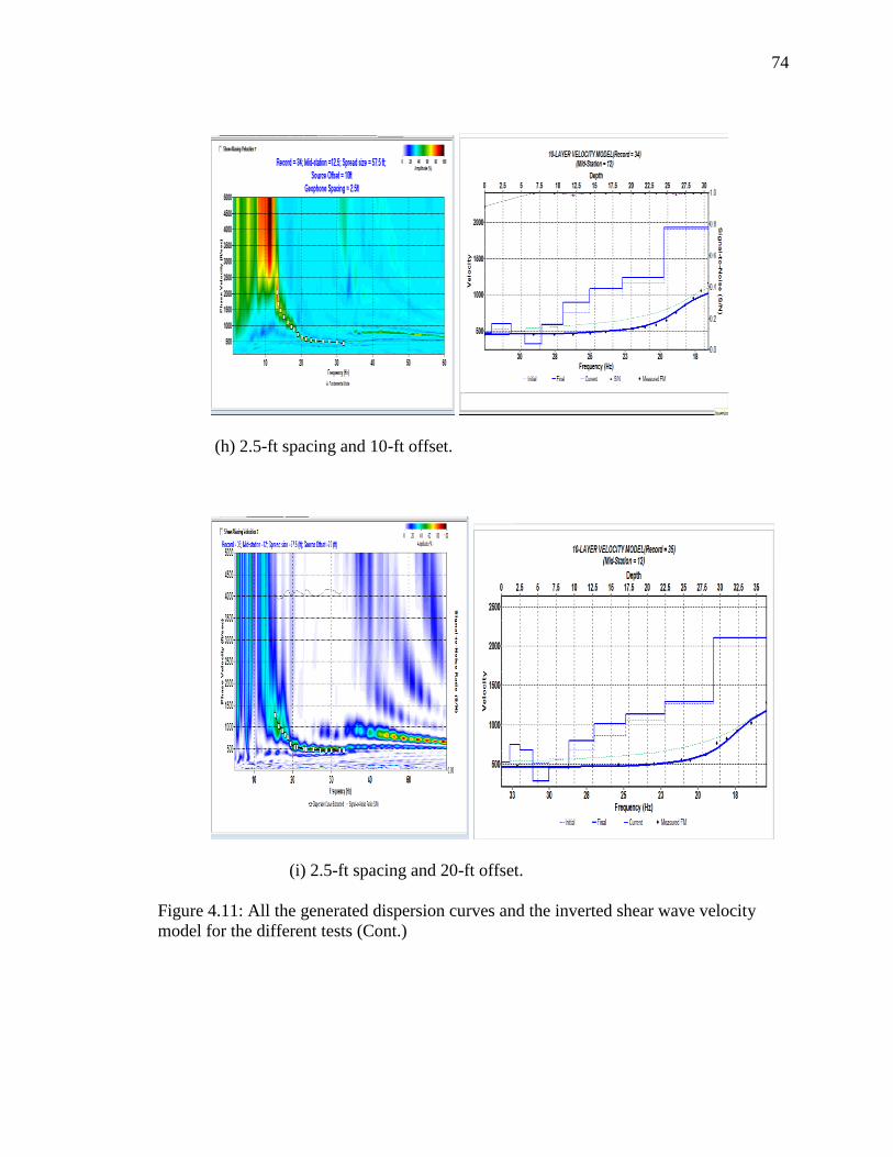
74
(h) 2.5-ft spacing and 10-ft offset.
(i) 2.5-ft spacing and 20-ft offset.
Figure 4.11: All the generated dispersion curves and the inverted shear wave velocity
model for the different tests (Cont.)

75
(j) 2.5-ft spacing and 30-ft offset.
(k) 2.5-ft spacing and 40-ft offset.
Figure 4.11: All the generated dispersion curves and the inverted shear wave velocity
model for the different tests (Cont.)

76
(l) 2.5-ft spacing and 50-ft offset.
(m) 5-ft spacing and 0-ft offset.
Figure 4.11: All the generated dispersion curves and the inverted shear wave velocity
model for the different tests (Cont.)

77
(n) 5-ft spacing and 10-ft offset.
(o) 5-ft spacing and 20-ft offset.
Figure 4.11: All the generated dispersion curves and the inverted shear wave velocity
model for the different tests (Cont.)

78
(p) 5-ft spacing and 30-ft offset.
(q) 5-ft. spacing and 40-ft offset.
Figure 4.11: All the generated dispersion curves and the inverted shear wave velocity
model for the different tests (Cont.)

79
(r) 5-ft spacing and 50-ft offset.
(s) 7.5-ft. Spacing and 0-ft offset.
Figure 4.11: All the generated dispersion curves and the inverted shear wave velocity
model for the different tests (Cont.)
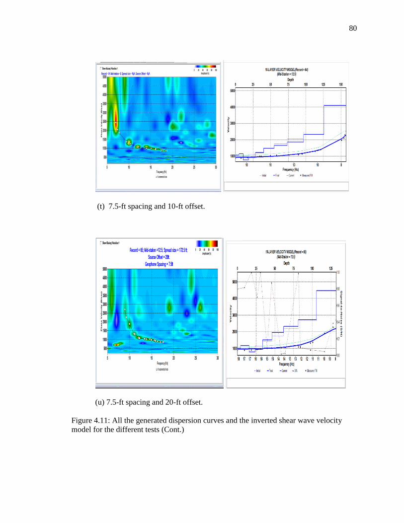
80
(t) 7.5-ft spacing and 10-ft offset.
(u) 7.5-ft spacing and 20-ft offset.
Figure 4.11: All the generated dispersion curves and the inverted shear wave velocity
model for the different tests (Cont.)

81
(v) 7.5-ft spacing and 30-ft offset.
(w) 7.5-ft spacing and 40-ft offset.
Figure 4.11: All the generated dispersion curves and the inverted shear wave velocity
model for the different tests (Cont.)

82
(x) 7.5-ft spacing and 50-ft offset.
(y) 10-ft spacing and 0-ft offset.
Figure 4.11: All the generated dispersion curves and the inverted shear wave velocity
model for the different tests (Cont.)

83
(z) 10-ft spacing and 10-ft offset.
(aa) 10-ft spacing and 20-ft offset.
Figure 4.11: All the generated dispersion curves and the inverted shear wave velocity
model for the different tests (Cont.)

84
(ab) 10-ft spacing and 30-ft offset.
(ac) 10-ft spacing and 40-ft offset.
Figure 4.11: All the generated dispersion curves and the inverted shear wave velocity
model for the different tests (Cont.)

85
(ad) 10-ft spacing and 50-ft offset.
Figure 4.11: All the generated dispersion curves and the inverted shear wave
velocity model for the different tests (Cont.)
4.4 ELECTRICAL RESISTIVITY TOMOGRAPHY (ERT)
4.4.1 Site Setup. Two measuring tapes were used to measure out the required
distance approximately 415- ft. along a flat surface on the site. NW-SE trend was chosen
because it makes room for the required length of array. After measuring out the required
length, metal stakes were installed at 5-ft. interval along the array making it 84 metal
stakes which covered the array length of 415-ft. The installation of the stakes was
supervised to make sure they were installed about half of the length of the stakes deep
inside the ground. Then four cables each consists of 20 electrodes were spread along the
array and each electrode was attached to each metal stakes (84 electrodes attached to 84
metal stakes) the four cable are connected to each other with a connector at both ends of
the cable. The first two cables were connected to each other and the last two were also
connected to each other, then the tail of the first two cables was connected to the switch

86
box also the head of the last two cables was connected to the switch box. The switch box
has two Amphenol (male and female) connectors (black plastic type) and two female
MS3476L18-32S connectors (metal type. The Amphenol connectors are used to connect
the switch box to the SuperSting instrument or daisy-chaining to other switch boxes to
control more electrodes. The MS3476L18-32S are used to connect the electrodes to the
instrument, use mating connector MS3476L18-32P. The connector marked “Low address
cable” is used to address electrodes 1-42. Pin 1 of the connector should be connected to
electrode 1, pin 2 to electrode 2 and so on. The connector marked “High address cable” is
used to address electrodes 43-84. Pin 1 of the connector was connected to electrode 42,
pin 2 to electrode 43 and so on. An adapter delivered with the switch box was used for
connecting the female connector of a passive cable to the female connector of the switch
box. The SuperSting was powered by two external 12 V DC batteries which were in the
boost mode. The batteries are attached to the instrument using the power cable. When in
main mode, the power cable is connected to the connector marked “Power” on the
SuperSting front panel. The red and black Mueller clips were attached to the positive and
the negative poles, respectively, of a 12 V battery. Figure 4.12 below show the switch
box and how it can be connected to the SuperSting, while Figure 4.13 shows the array set
up for the data acquisition.
(a) Switch box (b) SuperSting, switch box and 12V battery
Figure 4.12: Switch box and SuperSting

87
Figure 4.13: Four ERT traverses (red) and two MASW traverses (blue)
4.4.2 Field Procedure and Equipment. The SuperSting Resistivity System,
produced by Advanced Geosciences, Incorporated, was used to complete the survey. The
SuperSting R8 transmitter/receiver is a self-regulated eight channel digital volt meter,
capable of transferring up to two amps of current to the ground. With auxiliary switch
boxes, the SuperSting R8 is capable of conducting multiple readings using a string of up
to 84 electrodes. The equipment was supplied with the SuperSting R8, 4electrode cables,
each cable with 21 electrodes and 84 steel stakes. The SuperSting R8 system requires an
external 12 volt battery source; however, the performance of the equipment can be
optimized by using a pair, volt batteries connected in series (Advanced Geosciences,

88
Incorporated, 2006). Wet cell batteries were utilized for this application. The use of wet
cell batteries is preferred due to the ability to repeatedly drain the battery source and
recharge, within minimal impact to the battery core (Advanced Geosciences
Incorporated, 2008). The SuperSting R8 requires commands in order to properly trigger
electrodes for current induction and measurement of potential difference (Advanced
Geosciences Incorporated, 2008).
AGI Administrator software package, provided with the SuperSting Resistivity
System, allows the user to input array parameters to model resulting survey
psuedosections. The generated model will give the user an estimate of penetration depth,
data point coverage, and an estimation of time required to perform the survey. An
example of a generated psuedosection is provided in Figure 4.14. After an array
configuration is created, the user can create a unit less command file usable by the
SuperSting R8 transmitter/receiver. Another notable feature of the AGI Administrator
software is the ability to reverse the array direction, so that points are collected starting
from the end of the electrode string and progresses towards the first electrode in the array.
This progression is advantageous during a roll-along survey. The SuperSting R8 stores all
measurements of current and potential difference during the course of a survey. Each
measurement is coordinated with the address of the four electrodes associated with the
respective reading. With the capability of referencing coordinate or nodal locations of
past readings, the equipment can conclude a survey once all readings within a new
domain are acquired. By not overlapping existing data, the use of a reverse array provides
an efficient means of surveying and data storage for roll along applications (Advanced
Geosciences Incorporated, 2008).

89
For the purposes, of this survey, a dipole-dipole array was selected due to the
need for high lateral resolution and the relatively shallow depth of interest approximately
50-feet. The array was modeled in the AGI Administrator program, and then transferred
to the SuperSting R8 equipment for surveying purposes.
Figure 4.14: SuperSting Manager App, Plot pseudo section (Advanced
Geosciences Incorporated, 2008).
4.4.3 Data Acquisition. Consideration was given to the desired resolution, depth
of investigation, and available equipment. For the purposes of this study it was
determined that an interval spacing of 5 feet would adequately profile the bedrock as well
as the surficial materials. It was estimated that for electrodes, at an interval spacing of 5
feet, the approximate depth of penetration would be approximately 83 feet. This is based
on the assumption that the penetration depth is approximately 20 percent of the survey
length (Advanced Geosciences Incorporated, 2008). Each run would cover 415 linear feet

90
of the site. It should be noted that the AGI Administrator program generates a generic
command file which can be used with any given interval spacing (Figure 4.15)
For the purpose of this research, ERT data was acquired along four different
traverses trending NW-SE in order to have more coverage of the study area. Each of the
traverses is 20-ft apart from the other and the same array configurations were used for all
of the traverses.
(a) Set up
(b) Acquisition in progress.
Figure 4.15: Equipment set up for the ERT acquisition

91
4.4.4 Data Processing and Inversion. The raw data stored in the SuperSting R8
must be extracted and converted into a form suitable for processing. The AGI
Administrator software is used to download and covert field data into a form readable for
the AGI EarthImager 2D analysis software. In the raw form, measurements of apparent
resistivity can be plotted into the respective psuedosection. The EarthImager 2D software
uses the measured apparent resistivity psuedosection during the inversion process to
recreate an earth model fitting the conductive characteristics of the recorded raw model.
The default model used to begin the inversion process is a homogenous half-space with
an assigned resistivity equivalent to measured apparent resistivity values, in log form.
Other models may be used to begin the inversion by manual selecting available user-
defined functions (Advanced Geosciences, Incorporated, 2009).
The inversion process is iterative in two ways. First, EarthImager uses an iterative
routine to develop a matching earth model, using an error tolerance or maximum number
of iterations as criteria for terminating the inversion. Secondly, if the level of error in a
given model is beyond acceptable limits (i.e. root mean square or L2 Normalization
terms), the raw data can be evaluated to determine whether outlier measurements are
causing unwanted error in the inverted model. Disruptive points, or noise, can result from
cultural conditions present at the time of the survey, recordings of negative values, or
malfunctioning equipment. Corrupting data points can be isolated by using the misfit
histogram generated in the EarthImager program, manually eliminating data points in the
psuedosection or by suppressing the readings collected from particular electrodes. The
iteration process can stop when the user is satisfied that the represented model
demonstrates the subsurface condition, within the accepted error tolerances for the survey

92
(Advanced Geosciences Incorporated, 2009). Figure 4.16 below show all the
pseudosections and data points generated for the ERT traverses while Figure 4.17 show
final the inversion results for the four ERT traverses.
(a) ERT line 1 showing all the data points and 84 electrodes
(b) ERT line 2 showing all the data points and 84 electrodes.
Figure 4.16: Pseudo sections and data points generated for the ERT traverses

93
(c) ERT line 3 showing all the data points and 84 electrodes
(d) ERT line 4 showing all the data points and 84 electrodes.
Figure 4.16: Pseudo sections and data points generated for the ERT traverses (Cont.)
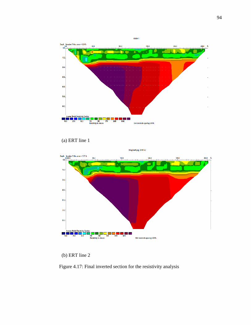
94
(a) ERT line 1
(b) ERT line 2
Figure 4.17: Final inverted section for the resistivity analysis

95
(c) ERT line 3
(d) ERT line 4
Figure 4.17: Final inverted section for the resistivity analysis (Cont.)
Furthermore, data points from four different ERT lines were collated to generate
three dimensional model (3D) using Voxler 3 software produced by Golden software Inc.

96
Voxler 3 creates powerful, fast, customized 3D images of any scientific data, it is user
friendly and easy to import data in a multitude of file formats to create stunning models
that visualize the relationships across your data set. This robust, yet user-friendly
program gives you the power to display your data in a variety of formats and colors,
capture video animation of your moving model, and select from several image and data
export options (Golden Software, Inc., 2013). Voxler gives you full control of your 3D
data. You can filter anomalies, duplicates, or areas you want eliminated. Interactively
manipulate your data while viewing the results, and personalize Voxler with a variety of
settings. It offers a multitude of computational modules and graphics display modules
that will simply get your modeling. Figure 4.18 show 3D model for all the four lines of
ERT generated with Voxler 3 software.
Figure 4.18: 3-D ERT Model generate with Voxler software. (a) Inclined view

97
(b) Lateral view.
(c) Orthogonal view.
Figure 4.18: 3-D ERT Model generate with Voxler software (Cont.)

98
4.5 CONCLUSIONS
These tests were conducted to determine the optimum acquisition
parameters (source offset and receiver spacing) for MASW data collection along with the
accuracy of the MASW dispersion curves and Vs profiles when compared to the 2D and
3D electrical resistivity tomography.

99
5. RESULTS
5.1 OVERVIEW
The MASW results from the data collected will be presented herein. My
concentration will be focused on results from different geophone spacing and offset
distance and their respective frequency ranges, phase velocities and depth of
investigation. The results are presented in a tabular form that compare the surface wave
dispersion curves obtained from various source offset distances and receiver spacings,
while keeping the other parameters unchanged. The dispersion curve result presented
herein are the same with the generated dispersion curves and shear wave velocity profiles
presented in chapter four. Also results from the final inverted section for the resistivity
analysis for ERT traverses will be presented as well.
Finally, results from muting as a processing tool will presented with emphasis on
the importance and limitations of muting.
5.2 RESULTS FROM MASW DATA
Results from dispersion curves and shear wave velocity profiles for all the tested
parameters are presented in Table 5.1 below. The discussion will be focused on the
comparison of these parameters (Geophone spacing and Offset distances) with respect to
frequency range, phase velocity range, depth to top of bedrock and the maximum depth
of investigation. From the overall dispersion curves and shear wave velocity profiles, the
shear wave velocity of the rock was set to be 1250-ft/sec and the fundamental mode

100
ranges from 15Hz to 32 Hz, while that phase velocity for the fundamental mode ranges
from 500-ft/sec to 1500-ft/sec.
(i) 1-ft Geophone Spacing
At 1-ft geophone spacing and 0-ft offset, the frequency range picked from the
dispersion curve is 55Hz to 110Hz, phase velocity ranges from 1000-ft/sec to 1350-ft/sec.
Velocity model could not be generated because fundamental modes could not be picked.
The result shows that the frequency range picked were not fundamental modes and phase
velocity range was high, there by depicting higher mode. The velocity model was
inaccurate; it was only included here to show problems that arise if higher modes are
picked.
For 1-ft geophone spacing and 10-ft offset, the frequency ranges from 15Hz to
30Hz, phase velocity ranges from 400-ft/sec to 1500-ft/sec, depth to bedrock is 17.5-ft
and the maximum depth of investigation is 37-ft. The frequency range picked fall within
the fundamental mode likewise the phase velocity ranges.
When using 1-ft geophone spacing and 20-ft offset, frequency ranges from 15Hz
to 20Hz, phase velocity ranges from 400-ft/sec to 1600-ft/sec, depth to bedrock is 17.5-ft
and the maximum depth of investigation is 50-ft. The frequency range picked fall within
the fundamental mode likewise the phase velocity ranges.
For 1-ft geophone spacing and 30-ft offset, the frequency ranges from 20Hz to
30Hz, phase velocity ranges from 500-ft/sec to 1450-ft/sec, depth to bedrock is 14-ft and
the maximum depth of investigation is 22.5-ft. The frequency range picked were not
fundamental mode likewise the phase velocity ranges.

101
For 1-ft geophone spacing and 40-ft receiver offset, the frequency ranges from
15Hz to 30Hz, phase velocity ranges from 1450-ft/sec to 1500-ft/sec, depth to bedrock is
19.5-ft and the maximum depth of investigation is 42.5-ft. The frequency range picked
fall within the fundamental mode likewise the phase velocity ranges.
Finally, 1-ft geophone spacing and 50-ft receiver offset, the frequency ranges
from 15Hz to 30Hz, phase velocity ranges from 500-ft/sec to 1500-ft/sec, depth to
bedrock is 16-ft and the maximum depth of investigation is 35-ft. The frequency range
picked fall within the fundamental mode likewise the phase velocity ranges.
(ii) 2.5-ft Geophone Spacing
At 0-ft receiver offset, the frequency ranges from 15Hz to 30Hz, phase velocity
ranges from 500-ft/sec to 1500-ft/sec, depth to bedrock is 18-ft and the maximum depth
of investigation is 38-ft. The frequency range picked fall within the fundamental mode
likewise the phase velocity ranges.
At 10-ft receiver offset, the frequency ranges from 15Hz to 32Hz, phase velocity
ranges from 500-ft/sec to 1500-ft/sec, depth to bedrock is 19-ft and the maximum depth
of investigation is 31-ft. The frequency range picked fall within the fundamental mode
likewise the phase velocity ranges.
At 20-ft receiver offset, the frequency ranges from 15Hz to 33Hz, phase velocity
ranges from 500-ft/sec to 1600-ft/sec, depth to bedrock is 22.5-ft and the maximum depth
of investigation is 38-ft. The frequency range picked fall within the fundamental mode
likewise the phase velocity ranges.
At 30-ft receiver offset, the frequency ranges from 15Hz to 30Hz, phase velocity
ranges from 500-ft/sec to 1500-ft/sec, depth to bedrock is 21-ft and the maximum depth
102
of investigation is 35-ft. The frequency range picked fall within the fundamental mode
likewise the phase velocity ranges.
At 40-ft receiver offset, the frequency ranges from 15Hz to 33Hz, phase velocity
ranges from 500-ft/sec to 1500-ft/sec, depth to bedrock is 23-ft and the maximum depth
of investigation is 37-ft. The frequency range picked fall within the fundamental mode
likewise the phase velocity ranges.
At 50-ft receiver offset, the frequency ranges from 18Hz to 35Hz, phase velocity
ranges from 500-ft/sec to 1000-ft/sec, depth to bedrock is 15-ft and the maximum depth
of investigation is 27-ft. The frequency range picked fall within the fundamental mode
likewise the phase velocity ranges.
(iii) 5-ft Geophone Spacing
At 0-ft receiver offset, the frequency ranges from 13Hz to 35Hz, phase velocity
ranges from 500-ft/sec to 1500-ft/sec, depth to bedrock is 15-ft and the maximum depth
of investigation is 55-ft. The frequency range picked fall within the fundamental mode
likewise the phase velocity ranges.
At 10-ft receiver offset, the frequency ranges from 15Hz to 28Hz, phase velocity
ranges from 500-ft/sec to 1400-ft/sec, depth to bedrock is 18-ft and the maximum depth
of investigation is 38-ft. The frequency range picked fall within the fundamental mode
likewise the phase velocity ranges.
At 20-ft receiver offset, the frequency ranges from 10Hz to 30Hz, phase velocity
ranges from 500-ft/sec to 2000-ft/sec, depth to bedrock is 20-ft and the maximum depth
of investigation is 80-ft. The frequency range picked fall within the fundamental mode
likewise the phase velocity ranges.

103
At 30-ft receiver offset, the frequency ranges from 15Hz to 25Hz, phase velocity
ranges from 500-ft/sec to 1500-ft/sec, depth to bedrock is 15-ft and the maximum depth
of investigation is 40-ft. The frequency range picked fall within the fundamental mode
likewise the phase velocity ranges.
At 40-ft receiver offset, the frequency ranges from 12Hz to 25Hz, phase velocity
ranges from 500-ft/sec to 2000-ft/sec, depth to bedrock is 20-ft and the maximum depth
of investigation is 80-ft. The frequency range picked fall within the fundamental mode
likewise the phase velocity ranges.
At 50-ft receiver offset, the frequency ranges from 15Hz to 23Hz, phase velocity
ranges from 500-ft/sec to 1500-ft/sec, depth to bedrock ranges 19-ft and the maximum
depth of investigation is 55-ft. The frequency range picked fall within the fundamental
mode likewise the phase velocity ranges.
(iv) 7.5-ft Geophone Spacing
At 0-ft receiver offset, the frequency ranges from 10Hz to 18Hz, phase velocity
ranges from 1000-ft/sec to 2000-ft/sec, depth to bedrock is 37-ft and the maximum depth
of investigation is 80-ft. The frequency range picked were not fundamental mode
likewise the phase velocity ranges.
At 10-ft receiver offset, the frequency ranges from 5Hz to 18Hz, phase velocity
ranges from 900-ft/sec to 2500-ft/sec, depth to bedrock is 26-ft and the maximum depth
of investigation is 150-ft. The frequency range picked were not fundamental mode
likewise the phase velocity ranges.
At 20-ft receiver offset, the frequency ranges from 8Hz to 18Hz, phase velocity
ranges from 900-ft/sec to 2600-ft/sec, depth to bedrock is 30-ft and the maximum depth
104
of investigation is 130-ft. The frequency range picked were not fundamental mode
likewise the phase velocity ranges.
At 30-ft receiver offset, the frequency ranges from 12Hz to 18Hz, phase velocity
ranges from 900-ft/sec to 1500-ft/sec, depth to bedrock is 36-ft and the maximum depth
of investigation is 60-ft. The frequency range picked were not fundamental mode
likewise the phase velocity ranges.
At 40-ft receiver offset, the frequency ranges from 10Hz to 18Hz, phase velocity
ranges from 900-ft/sec to 1500-ft/sec, depth to bedrock is 24-ft and the maximum depth
of investigation is 70-ft. The frequency range picked were not fundamental mode
likewise the phase velocity ranges.
At 50-ft receiver offset, the frequency ranges from 12Hz to 18Hz, phase velocity
ranges from 900-ft/sec to 1200-ft/sec, depth to bedrock is 35-ft and the maximum depth
of investigation is 43-ft. The frequency range picked were not fundamental mode
likewise the phase velocity ranges.
(v) 10-ft Geophone Spacing
At 0-ft receiver offset, the frequency ranges from 9.5Hz to 18Hz and phase
velocity ranges from 1500-ft/sec to 2000-ft/sec. shear wave velocity profile of this data
could not be generated hence, no information regarding depth to bedrock nor the
maximum depth of investigation. The frequency range picked were not fundamental
mode likewise the phase velocity ranges.
At 10-ft receiver offset , the frequency ranges from 8Hz to 12Hz , phase velocity
ranges from 1000-ft/sec to 1800-ft/sec, depth to bedrock is 10-ft and the maximum depth

105
of investigation is 86-ft. The frequency range picked were not fundamental mode
likewise the phase velocity ranges.
At 20-ft receiver offset, the frequency ranges from 5Hz to 8Hz, phase velocity
ranges from 600-ft/sec to 800-ft/sec, depth to bedrock is 45-ft and the maximum depth of
investigation is 70-ft. The frequency range picked were not fundamental mode likewise
the phase velocity ranges.
At 30-ft receiver offset, the frequency ranges from 7Hz to 9Hz, phase velocity
ranges from 600-ft/sec to 800-ft/sec, depth to bedrock is 38-ft and the maximum depth of
investigation is 47.5-ft. The frequency range picked were not fundamental mode likewise
the phase velocity ranges.
At 40-ft receiver offset, the frequency ranges from 3Hz to 5Hz, phase velocity
ranges from 600-ft/sec to 1000-ft/sec, depth to bedrock is 100-ft and the maximum depth
of investigation is 125-ft. The frequency range picked were not fundamental mode
likewise the phase velocity ranges.
Finally at 50-ft receiver offset, the frequency ranges from 5Hz to 7Hz, phase
velocity ranges from 400-ft/sec to 1100-ft/sec, depth to bedrock is 55-ft and the
maximum depth of investigation is 90-ft. The frequency range picked were not
fundamental mode likewise the phase velocity ranges. Results from all the dispersion
curves and generated shear wave velocity profiles are listed in the Table 5.1 below.

106
Table 5.1: Results from all the dispersion curves and generated shear wave velocity
profiles.
S/N
Spacing
(Ft.)
Offset
(Ft.)
Source
(lb)
Frequency
Range
(Hz)
Phase
Velocity
(Ft./sec)
Depth to
bedrock(
Ft.)
Max.
depth
(Ft.) Quality
1 1 0 20 55 -110 1000- 1350 - - N/A
2 1 10 20 15 - 30 400 -1500 17.5 37 Good quality
3 1 20 20 15 - 20 400 -1600 17.5 50 Good quality
4 1 30 20 20 - 30 500 -1450 14 22.5 Good quality
5 1 40 20 15 - 30 1450-1500 19.5 42.5 Good quality
6 1 50 20 15 - 30 500 -1500 16 35 Good quality
7 2.5 0 20 15 - 30 500 - 1600 18 38 Good quality
8 2.5 10 20 15 - 32 500 - 1500 19 31 Good quality
9 2.5 20 20 15 - 33 500 -1600 22.5 38 Good quality
10 2.5 30 20 15 - 30 500 - 1500 21 45 Good quality
11 2.5 40 20 15 - 33 500 - 1500 22.5 37 Good quality
12 2.5 50 20 18 - 35 500 - 1000 21 27 Good quality
13 5 0 20 13 - 35 500 - 1500 15 55 Good quality
14 5 10 20 15 - 28 500 - 1400 18 38 Good quality
15 5 20 20 10 - -30 500 - 2000 20.5 80 Excellent quality
16 5 30 20 15 - 25 500 - 1500 15 40 God quality
17 5 40 20 12 - 25 500 - 2000 20 80 Excellent quality
18 5 50 20 15 - 23 500 - 1500 19 55 Excellent quality
19 7.5 0 20 10 -18 1000-2000 37 80 Poor quality
20 7.5 10 20 5 - 18 900-2500 26 150 Poor quality
21 7.5 20 20 8 - 18 900 - 2600 30 130 Poor quality
22 7.5 30 20 12 - 18 900-1500 36 60 Poor quality
23 7.5 40 20 10 - 18 900 - 1500 24 70 Poor quality
24 7.5 50 20 12 -18 900 - 1200 35 43 Poor quality
25 10 10 20 8 - 12 1000-1800 10 86 Poor quality
27 10 20 20 5 - 8 600 -800 45 70 Poor quality
28 10 30 20 7 - 9 600 - 800 38 47.5 Poor quality
29 10 40 20 3 - 5 600 - 1000 100 125 Poor quality
30 10 50 20 5 - 7 400 - 1100 55 90 Poor quality
5.3 RESULTS FROM ERT DATA
Results for all the four ERT traverses show that top layer of the site are mainly
alluvium with pockets of consolidated sand dominating at the western part of the array.

107
Top of bedrock in this site is gradational ranging from 17-ft to the excess of 22-ft with
resistivity ranging from 388 Ohm-meters to excess of 615 Ohm-meters. There is an
indication of a low resistivity zone at the western part of the array, this could depict moist
soil which is deposited by the Corn creek which flows 20-ft away from the array. Also
parts of the bedrock at the western part of the array have been eroded thereby deepening
the bedrock in that area. Figure 5.1 to Figure 5.4 show the details of the ERT results,
while Figure 5.5 confirmed the assumption that the top of bedrock ranges from 17-ft to
23-ft.
Figure 5.1: Final inverted section for the resistivity analysis for ERT line 1 showing top
of bedrock in black dotted lines, pockets of consolidated sand layer, moist soil and very
intact bedrock.
Top of
bedrock
Pockets of consolidated sand
Moist soil
Very Intact bedrock

108
Figure 5.2: Final inverted section for the resistivity analysis for ERT line 2 showing top
of bedrock in black dotted lines, pockets of consolidated sand layer, moist soil and very
intact bedrock.
Figure 5.3: Final inverted section for the resistivity analysis for ERT line 3 showing top
of bedrock in black dotted lines, pockets of consolidated sand layer, moist soil and very
intact bedrock.

109
Figure 5.4: Final inverted section for the resistivity analysis for ERT line 4 showing top
of bedrock in black dotted lines, pockets of consolidated sand layer, moist soil and very
intact bedrock.
Figure 5.5: 3-D model generated by combining the four ERT traverses using Voxler
software.
5.4 MUTING
The purpose of muting is to remove specific seismic energy (e.g., dispersion
curve), which arrives in specific time frame as a result of its velocity of propagation
characteristics (Miller, Ivanov, et al., 2001). For example, in the context of the surface
110
wave method, part of the higher mode energy that propagates faster than the fundamental
mode will arrive first on the seismic record. Thus, the fundamental mode energy will
begin to appear after certain time, after the arrival of the higher modes. The main
condition for the application of the muting method for event separation is the observation
of different apparent velocity trends on the raw seismic data. In this research, I
demonstrate a method for removing components of seismic wave-field, mainly higher
modes of surface wave energy that appear as noise in the phase-velocity – frequency
domain, in which dispersion curves are estimated. After proper muting, the quality and
observation range of the desired mode (i.e., fundamental mode) improve significantly.
The basis for the application of the method is eliminating certain arrival-time
ranges in the offset-time domain, within which certain wave-field components arrive as a
result of their overall propagation velocity. For example, higher mode components are
expected to arrive earlier on the shot record because of their velocity than the
fundamental mode. After muting, the corresponding phase-velocity – frequency domain
will lack the noisy event (which appears at a different arrival-time range). The proposed
filtering method is effective when it is applied on a seismic shot gathers that have more
than one and clearly different surface-wave velocity trends, which can be
straightforwardly distinguished.
To show the effect of muting, muting method was applied to shot gather from 2.5-
ft geophone spacing at 0-ft receiver offset Figure 5.6 and Figure 5.7 show their dispersion
curves before and after muting was applied.

111
(a) Before Muting
(b) After Muting.
Figure 5.6: Raw shot gather from a 2.5-ft geophone spacing and 0-ft receiver
offset before and after muting

112
(a) Before Muting.
(b) After Muting.
Figure 5.7: Dispersion curve for 2.5-ft spacing and 0-ft offset

113
5.4.1 Results from Muting. From the example above, it can be seen that surface-
wave energy dominates the seismic record (Fig 5.6). The dispersion curve reveals two
dispersive events of the surface-wave, the fundamental mode and a high mode (Fig.
5.6c). The fundamental mode can be observed within a narrow frequency range between
10 and 30 Hz (and velocity between 500-1600-ft/sec) while the higher mode dominates a
wide frequency range between 25 and 50Hz (and velocities between 700-1500-ft/sec).
Efforts to observe the fundamental mode between 15 and 50 Hz by boosting the
amplitude of the phase-velocity – frequency spectrum did not bring any success. Thus,
the higher-mode energy is significantly higher, and it inhibits the estimation of the
fundamental mode dispersion-curve trend above 15 Hz. There are 3 stages to apply
muting successfully in MASW processing. The first stage is the estimation of the phase
velocities of the fundamental mode of the surface waves in the low-frequency zone. The
phase velocity of the fundamental mode ranges from 400 to 1500-ft/sec. The second stage
is the muting of the shot gathers from energy dominated by the higher modes and
estimating the phase velocities of the fundamental mode of the surface waves in this
frequency range (fig 5.6b), which is no longer dominated by higher modes in the raw
shot gathers. I muted the surface wave energy below 335-ft/sec and above 1600-ft/sec.
The final step is to combine the two curves into a single dispersion curve using the
overlapping zone for confirmation of the evaluation and ignoring the steep velocity-
gradient portion (at lower frequencies) of the second curve. The acquired fundamental
mode dispersion curve now spans over a wide frequency range (10-40 Hz). Thereby
eliminating the higher mode energy of the surface wave in the range 15 – 40 Hz in the
phase velocity – frequency domain and boosting the weaker fundamental mode energy

114
within the same frequency range (Fig. 5.6 d). The muting also has completely eliminated
the fundamental mode of the surface wave in the range of 5 – 10 Hz (Fig. 5.6c) that has
high phase velocity values which inhibit the estimation of the fundamental mode with
low phase velocity values. This however, was expected because the low frequency
components of the fundamental mode have velocities that are in the velocity range of the
muted high mode (Miller, Ivanov, et al., 2001).
5.4.2 Importance of Muting. Fundamental mode dispersion curve energy can be
boosted in the phase- velocity – frequency domain after examining a multichannel shot
record, recognizing and muting harmful higher mode dispersive energy in the shot record
domain. Also muting can significantly improve the bandwidth of the fundamental mode
and the dispersion curve picking when using MASW. The downside of muting is that it
introduces a high-velocity gradient feature at the low frequency end of the dispersion
curve, which is not present before muting. This artifact can be easily handled by using the
dispersion curve from the non-muted data that covers the same frequency range, so the
artificially high-velocity values can be ignored and are thus considered harmless (Miller,
Ivanov, et al., 2001).

115
6. DISCUSSIONS
6.1 OVERVIEW
Results from MASW data are compared herein with ERT data to determine their
accuracy in imaging the top of bedrock in the study area. The acoustic top of bedrock in
the study area is 1250-ft. /Sec while the resistivity of top of bedrock ranges from
388Ohms-meter to excess of 615 Ohms-meter. The estimated top of bedrock based on the
resistivity data shows that it ranges from 17-ft to 23-ft and the expected depth of
investigation would be 50-ft. In this section, results from the dispersion curves and shear
wave velocity profiles of the tested parameters (off set distances and geophone spacings)
will be compared with ERT results to determine their accuracy and variations in imaging
the top of bedrock and maximum depth of investigation in the study area.
6.2 COMPARISON OF MASW RESULTS WITH 2-D ERT RESULTS
(i) 1-ft Geophone Spacing
Now starting with 10-ft offset and 1-ft geophone spacing, the estimated top of
bedrock was 17.5-ft and the maximum depth of investigation would be 37-ft. This result
corresponds with the ERT result which shows that the top of bedrock ranges from 17-ft to
23-ft, but maximum depth of investigation would shallower (less than 50-ft.) which is the
targeted depth of investigation for this research. Therefore, these parameters would only
be useful for a shallower depth of investigation (about 35-ft).
When imaging the top of bedrock using 20-ft offset and 1-ft geophone spacing,
the estimated top of bedrock was 17.5-ft and the maximum depth of investigation would

116
be 50-ft. This result corresponds with the ERT result which shows that the top of bedrock
ranges from 17-ft to 23-ft. Also, the maximum depth of investigation would be 50-ft
which is the targeted depth of investigation for this research. Therefore, these parameters
would be useful and appropriate for mapping acoustic top of bedrock and image the
required depth of investigation in the study area.
Also, when imaging the top of bedrock using 30-ft offset and 1-ft geophone
spacing, the estimated top of bedrock was 14-ft and the maximum depth of investigation
would be 22-ft. This result does not corresponds with the ERT result which shows that
the top of bedrock ranges from 17-ft to 23-ft. Also, maximum depth of investigation
would be shallower (less than 50-ft.) which the targeted depth of investigation for this
research is. Therefore, these parameters would only be useful for a shallower depth of
investigation of about 20-ft.
When imaging the top of bedrock using 40-ft offset and 1-ft geophone spacing,
the estimated top of bedrock was 19.5-ft and the maximum depth of investigation would
be 42.5-ft. This result corresponds with the ERT result which shows that the top of
bedrock ranges from 17-ft to 23-ft, but maximum depth of investigation would be
shallower (less than 50-ft.) which is the targeted depth of investigation for this research.
Therefore, these parameters would only be useful for a shallower depth of investigation
(about 40-ft).
Finally, when imaging the top of bedrock using 50-ft offset and 1-ft geophone
spacing, the estimated top of bedrock was 16-ft and the maximum depth of investigation
would be 35-ft. This result corresponds slightly with the ERT result which shows that the
top of bedrock ranges from 17-ft to 23-ft, but maximum depth of investigation would be

117
shallower (less than 50-ft.) which is the targeted depth of investigation for this research.
Therefore, these parameters would only be useful for a shallower depth of investigation
(about 30-ft).
(ii) 2.5-ft Geophone Spacing
When imaging the top of bedrock using 0-ft offset and 2.5-ft geophone spacing,
the estimated top of bedrock was 18-ft and the maximum depth of investigation would be
38-ft. This result corresponds with the ERT result which shows that the top of bedrock
ranges from 17-ft to 23-ft, but maximum depth of investigation would be shallower (less
than 50-ft.) which is the targeted depth of investigation for this research. Therefore, these
parameters would only be useful for a shallower depth of investigation (about 35-ft).
When imaging the top of bedrock using 10-ft offset and 2.5-ft geophone spacing,
the estimated top of bedrock was 19-ft and the maximum depth of investigation would be
31-ft. This result corresponds with the ERT result which shows that the top of bedrock
ranges from 17-ft to 23-ft, but maximum depth of investigation would be shallower (less
than 50-ft.) which is the targeted depth of investigation for this research. Therefore, these
parameters would only be useful for a shallower depth of investigation (about 30-ft).
When imaging the top of bedrock using 20-ft offset and 2.5-ft geophone spacing,
the estimated top of bedrock was 22.5-ft and the maximum depth of investigation would
be 38-ft. This result corresponds with the ERT result which shows that the top of bedrock
ranges from 17-ft to 23-ft, but maximum depth of investigation would be shallower (less
than 50-ft.) which is the targeted depth of investigation for this research. Therefore these
parameters would only be useful for a shallower depth of investigation (about 35-ft).

118
When imaging the top of bedrock using 30-ft offset and 2.5-ft geophone spacing,
the estimated top of bedrock was 21-ft and the maximum depth of investigation would be
35-ft. This result corresponds with the ERT result which shows that the top of bedrock
ranges from 17-ft to 23-ft, but maximum depth of investigation would be shallower (less
than 50-ft.) which is the targeted depth of investigation for this research. Therefore these
parameters would only be useful for a shallower depth of investigation (about 30-ft).
When imaging the top of bedrock using 40-ft offset and 2.5-ft geophone spacing,
the estimated top of bedrock was 23-ft and the maximum depth of investigation would be
37-ft. This result corresponds with the ERT result which shows that the top of bedrock
ranges from 17-ft to 23-ft, but maximum depth of investigation would be shallower (less
than 50-ft.) which is the targeted depth of investigation for this research. Therefore, these
parameters would only be useful for a shallower depth of investigation (about 35-ft).
When imaging the top of bedrock using 50-ft offset and 2.5-ft geophone spacing,
the estimated top of bedrock was 15-ft and the maximum depth of investigation would be
27-ft. This result does not corresponds with the ERT result which shows that the top of
bedrock ranges from 17-ft to 23-ft, but maximum depth of investigation would be
shallower (less than 50-ft.) which is the targeted depth of investigation for this research.
Therefore, these parameters would only be useful for a shallower depth of investigation
(about 25-ft).
(iii) 5-ft Geophone Spacing
When imaging the top of bedrock using 0-ft offset and 5-ft geophone spacing, the
estimated top of bedrock was 15-ft and the maximum depth of investigation would be 55-
ft. This result does not correspond with the ERT result which shows that the top of
119
bedrock ranges from 17-ft to 23-ft, but maximum depth of investigation would be
appropriate and accurate (more than 50-ft.) which is the targeted depth of investigation
for this research. Therefore, these parameters would be appropriate for imaging a deeper
depth of investigation (more than 50-ft).
When imaging the top of bedrock using 10-ft offset and 5-ft geophone spacing,
the estimated top of bedrock was 18-ft and the maximum depth of investigation would be
38-ft. This result corresponds with the ERT result which shows that the top of bedrock
ranges from 17-ft to 23-ft, but maximum depth of investigation would be shallower (less
than 50-ft.) which is the targeted depth of investigation for this research. Therefore, these
parameters would only be useful for a shallower depth of investigation (about 35-ft).
When imaging the top of bedrock using 20-ft offset and 5-ft geophone spacing,
the estimated top of bedrock was 20-ft and the maximum depth of investigation would be
80-ft. This result corresponds with the ERT result which shows that the top of bedrock
ranges from 17-ft to 23-ft. Also, maximum depth of investigation would be appropriate
and accurate (more than 50-ft.) which is the targeted depth of investigation for this
research. Therefore, these parameters would be appropriate for imaging a deeper depth of
investigation (more than 50-ft).
When imaging the top of bedrock using 30-ft offset and 5-ft geophone spacing,
the estimated top of bedrock was 15-ft and the maximum depth of investigation would be
40-ft. This result does not correspond with the ERT result which shows that the top of
bedrock ranges from 17-ft to 23-ft, also, the expected maximum depth of investigation
would be shallower (less than 50-ft.) which is the targeted depth of investigation for this

120
research. Therefore, these parameters would be appropriate for imaging a shallower depth
of investigation (less than 40-ft).
When imaging the top of bedrock using 40-ft offset and 5-ft geophone spacing,
the estimated top of bedrock was 20-ft and the maximum depth of investigation would be
80-ft. This result corresponds with the ERT result which shows that the top of bedrock
ranges from 17-ft to 23-ft. Also, maximum depth of investigation would be appropriate
and accurate (more than 50-ft.) which is the targeted depth of investigation for this
research. Therefore, these parameters would be appropriate for imaging a deeper depth of
investigation (more than 50-ft).
When imaging the top of bedrock using 50-ft offset and 5-ft geophone spacing,
the estimated top of bedrock was 19-ft and the maximum depth of investigation would be
55-ft. This result corresponds with the ERT result which shows that the top of bedrock
ranges from 17-ft to 23-ft. Also, maximum depth of investigation would be appropriate
and accurate (more than 50-ft.) which is the targeted depth of investigation for this
research. Therefore, these parameters would be appropriate for imaging a deeper depth of
investigation (more than 50-ft).
(iv) 7.5-ft Geophone Spacing
When imaging the top of bedrock using 0-ft offset and 7.5-ft geophone spacing,
the estimated top of bedrock was 37-ft and the maximum depth of investigation would be
80-ft. This result does not corresponds with the ERT result which shows that the top of
bedrock ranges from 17-ft to 23-ft. But expected maximum depth of investigation would
be appropriate and accurate (more than 50-ft.) which is the targeted depth of investigation

121
for this research. Therefore, these parameters would be appropriate for imaging a deeper
depth of investigation (more than 50-ft).
When imaging the top of bedrock using 10-ft offset and 7.5-ft geophone spacing,
the estimated top of bedrock was 26-ft and the maximum depth of investigation would be
150-ft. This result does not corresponds with the ERT result which shows that the top of
bedrock ranges from 17-ft to 23-ft. But expected maximum depth of investigation would
be appropriate and accurate (more than 50-ft.) which is the targeted depth of investigation
for this research. Therefore, these parameters would be appropriate for imaging a deeper
depth of investigation (more than 50-ft).
When imaging the top of bedrock using 20-ft offset and 7.5-ft geophone spacing,
the estimated top of bedrock was 30-ft and the maximum depth of investigation would be
130-ft. This result does not corresponds with the ERT result which shows that the top of
bedrock ranges from 17-ft to 23-ft. But expected maximum depth of investigation would
be appropriate and accurate (more than 50-ft.) which is the targeted depth of investigation
for this research. Therefore, these parameters would be appropriate for imaging a deeper
depth of investigation (more than 50-ft).
When imaging the top of bedrock using 30-ft offset and 7.5-ft geophone spacing,
the estimated top of bedrock was 30-ft and the maximum depth of investigation would be
60-ft. This result does not corresponds with the ERT result which shows that the top of
bedrock ranges from 17-ft to 23-ft. But expected maximum depth of investigation would
be appropriate and accurate (more than 50-ft.) which is the targeted depth of investigation
for this research. Therefore, these parameters would be appropriate for imaging a deeper
depth of investigation (more than 50-ft).

122
When imaging the top of bedrock using 40-ft offset and 7.5-ft geophone spacing,
the estimated top of bedrock was 24-ft and the maximum depth of investigation would be
70-ft. This result does not corresponds with the ERT result which shows that the top of
bedrock ranges from 17-ft to 23-ft. But expected maximum depth of investigation would
be appropriate and accurate (more than 50-ft.) which is the targeted depth of investigation
for this research. Therefore, these parameters would be appropriate for imaging a deeper
depth of investigation (more than 50-ft).
When imaging the top of bedrock using 50-ft offset and 7.5-ft geophone spacing,
the estimated top of bedrock was 35-ft and the maximum depth of investigation would be
43-ft. This result does not corresponds with the ERT result which shows that the top of
bedrock ranges from 17-ft to 23-ft. Also, expected maximum depth of investigation
would be shallower (less than 50-ft.) which the targeted depth of investigation for this
research is. Therefore, these parameters would be appropriate for imaging a shallower
depth of investigation (less than 50-ft).
(v) 10-ft Geophone Spacing
When imaging the top of bedrock using 10-ft offset and 10-ft geophone spacing,
the estimated top of bedrock was 10-ft and the maximum depth of investigation would be
86-ft. This result does not correspond with the ERT result which shows that the top of
bedrock ranges from 17-ft to 23-ft, but maximum depth of investigation would be
appropriate and accurate (more than 50-ft.) which is the targeted depth of investigation
for this research. Therefore, these parameters would be appropriate for imaging a deeper
depth of investigation (more than 50-ft).

123
When imaging the top of bedrock using 20-ft offset and 10-ft geophone spacing,
the estimated top of bedrock was 45-ft and the maximum depth of investigation would be
70-ft. This result does not corresponds with the ERT result which shows that the top of
bedrock ranges from 17-ft to 23-ft. But expected maximum depth of investigation would
be appropriate and accurate (more than 50-ft.) which is the targeted depth of investigation
for this research. Therefore, these parameters would be appropriate for imaging a deeper
depth of investigation (more than 50-ft).
When imaging the top of bedrock using 30-ft offset and 10-ft geophone spacing,
the estimated top of bedrock was 38-ft and the maximum depth of investigation would be
47.5-ft. This result does not corresponds with the ERT result which shows that the top of
bedrock ranges from 17-ft to 23-ft. Also, expected maximum depth of investigation
would be shallower (less than 50-ft.) which the targeted depth of investigation for this
research is. Therefore, these parameters would be appropriate for imaging a shallower
depth of investigation (less than 50-ft).
When imaging the top of bedrock using 40-ft offset and 10-ft geophone spacing,
the estimated top of bedrock was 100-ft and the maximum depth of investigation would
be 125-ft. This result does not corresponds with the ERT result which shows that the top
of bedrock ranges from 17-ft to 23-ft. But expected maximum depth of investigation
would be appropriate and accurate (more than 50-ft.) which is the targeted depth of
investigation for this research. Therefore, these parameters would be appropriate for
imaging a deeper depth of investigation (more than 50-ft).
When imaging the top of bedrock using 50-ft offset and 10-ft geophone spacing,
the estimated top of bedrock was 55-ft and the maximum depth of investigation would be

124
90-ft. This result does not corresponds with the ERT result which shows that the top of
bedrock ranges from 17-ft to 23-ft. But expected maximum depth of investigation would
be appropriate and accurate (more than 50-ft.) which is the targeted depth of investigation
for this research. Therefore, these parameters would be appropriate for imaging a deeper
depth of investigation (more than 50-ft).
6.3 FINAL ANALYSIS
Analysis of the discussed are analyzed in this section based there appropriate
matches with the ERT results. The analyses are divided into three categories (Excellent,
Good and Poor) in Table 6.1
Table 6.1: Final result analysis for MASW and ERT testing
Excellent Quality
(Top of bedrock and
Max. depth of
investigation accurate
with ERT result)
Good Quality
(Top of bedrock is accurate
with ERT result but shallower
depth investigation)
Poor Quality
( Deeper depth of
investigation at deeper
top of bedrock)
Offset
(ft)
Spacing
(ft)
20 5
40 5
50 5
Offset (ft) Spacing (ft)
10 1
20 1
30 1
40 1
50 1
0 2.5
10 2.5
20 2.5
30 2.5
40 2.5
50 2.5
0 5
10 5
30 5
Offset
(ft)
Spacing
(ft)
0 7.5
10 7.5
20 7.5
30 7.5
40 7.5
50 7.5
10 10
20 10
30 10
40 10
50 10

125
7. CONCLUSIONS
The primary objective of this study was to image the subsurface of the study area
to 50-ft using Multichannel Analysis of Surface Waves and Electrical Resistivity
Tomography and compare the estimated top of bedrock from the MASW results and ERT
results. From the comparison of these results, the optimum acquisition parameters for the
MASW for this site would be selected based on how accurate they match with the ERT
results in estimating the top of bedrock and imaging a maximum depth of investigation of
50-ft.
Observations from the final analysis of the MASW results show
(1) Profile data from electrical resistivity and MASW analyses was
comparable with each other.
(2) Dissimilarities between MASW data and ERT data can exist due to the
heterogeneity of the earthen structure, as well as the resolution capabilities and data
smoothing associated with each method
(3) 1-ft geophone spacing at 20-ft offset distance, 5-ft geophone spacing at
20-ft offset and 5-ft geophone spacing at 40-ft offset distance were the most accurate
parameters because they corresponded with the ERT result for the estimation of top of
bedrock and also will be appropriate for imaging the subsurface to 50-ft.
(4) 2.5-ft geophone spacing at 0-ft, 10-ft, 20-ft, 30-ft, 40-ft, 50-ft offset
distance and 1-ft geophone spacing at 10-ft, 40-ft, 50-ft offset distance gave a good
quality result because they corresponded with the ERT result for the estimation of the top
of rock, but would not be advisable for imaging the subsurface more than 40-ft.

126
Conclusively, the most appropriate parameters for estimating the top of bedrock
and imaging the subsurface of this study area to 50-ft would be 5-ft geophone spacing at
20-ft offset and 5-ft geophone spacing at 40-ft offset distance. These parameters were
chosen as the optimum acquisition parameters for this site because they gave the accurate
top of bedrock and were able to image the subsurface at 50-ft.

127
8. RECOMMENDATIONS
The performance of similar analyses is needed in order to validate the primary
objective of this study. It is believed that future studies would benefit by utilizing and/or
incorporating the following measures in the methodology:
Perform all testing and data acquisition during the same analysis period to
limit any potential variations in site conditions.
Incorporate GPS and/or GIS information into data acquisition and
presentation of findings to enhance the location of survey features and testing results.
Higher source like drop source or vibrator should be used to enhance the
quality of the MASW data.
Borehole data should be available as a ground truth for estimating the top
of bedrock and calibrating MASW and ERT with borehole data would be highly
recommended.
On the basis of data that were acquired it is recommended that 2.5ft
spacing be used if depth of investigation is about 40ft, but if the depth of investigation is
about 80-ft, using a sledge hammer source then 5-ft geophone spacing at 20-ft shot-
receiver offset distance is recommended.

128
BIBIOGRAPHY
Advanced Geosciences Incorporated. "Workshop/Seminar on Resistivity
Imagining." Austin, April 29, 2008.
Advanced Geosciences, Inc. January 23, 2009.http://www.agiusa.com (accessed
April 16, 2009).
Advanced Geosciences, Incorporated. "Instruction Manual for the Super Sting
with Swift Automatic Resistivity and IP System." Austin, January 2006.
Callister Jr, William D. Fundamentals of Material Science and Engineering. New
York: John Wiley and Sons, Inc., 2001.
Clinton .M. Wood “The impact of source type, source offset, and receiver spacing
on experimental masw data at soft-over-stiff sites, Master’s degree thesis University of
Arkansas, 2009.
Geometrics Incorporated. "ES-3000, Geode, and Strata Visor NZ/NZC Operator's
Manual, P/N 28519-01 Rev K." San Jose, June 2003.
Gibson, Paul J, and Dorothy M George. Environmental Applications of
Geophysical Surveying Techniques. Hauppauge: Nova Science Publishers, 2003.
Golden Software, Inc. 2013. (http://www.goldensoftware.com/voxler-
videos/voxler-3-loading-and-visualizing-well-data?ml=1).
Hazmira Liyana (2013, December 13) Gujarat Earthquake [Web log
post].Retrieved May 3, 2015, from http://geohazardsearthquake.blogspot.com.
Ivanov, Julian, Choon Park, and Jianghai Xia. "MASW/Surfseis 2 Workshop."
Fort Worth: Kansas Geologic Survey, March 28, 2009.
Kearey, Brooks and Hill, 2002. Introduction to Geophysical Exploration.
Williston: Blackwell Publishing, 2002.
Loke, M.H. "Electrical Imaging Survey for Environmental and Engineering
Studies." 2000.
MASW to investigate subsidence in the Tampa, Florida area: Kansas Geological
Survey Open-file Report 99–33.2014.
Milson, John. Field Geophysics. New York: John Wiley & Sons, 1996.

129
Missouri Department of Natural Resources (FGDC-STD-001-1998) Geographic
Information System. Retrieved May 3, 2015, http://dnr.mo.gov/gis/geology.surficial.xml
Multichannel Analysis of Surface Waves (2013, March 13) Dispersion Analysis.
Retrieved May 3, 2015, from http://www.masw.com/DispersionAnalysis.html.
Nazarian, 1984; Nazarian S, Stokoe II KH. In situ shear wave velocities from
spectral analysis of surface waves. Proceedings of 8th Conference on Earthquake
Engineering, San Francisco, 1984. vol. 3. P.38-45.
Parasnis, D.S. Principles of Applied Geophysics. New York: Chapman & Hall,
1997.
Park CB, Miller RD, Xia J. Imaging dispersion curves of surface waves on
multichannel record. 68th Annual International Meeting, Society of Exploration
Geophysicists, Expanded Abstracts; 1998. p. 1377-1380.
Park CB, Miller RD, Xia J. Multichannel analysis of surface waves. Geophysics
1999; 64(3):800-808.
Park, Choon B, Miller, Richard D., Xia Jianghai. (1997) "Multi-Channel Analysis
of Surface Waves (MASW) a summary report of technical aspects, experimental results,
and perspective” Kansas Geological Survey Open-file Report #97-10.
Park, Choon B, Richard D Miller, Jianghai Xia, and Julian Ivanov. "MASW - An
easy seismic Method to map shear-wave velocity of the ground." Chun Cheon: Korean
Society of Engineering Geology, 2004.
Park, Choon B, Richard D Miller, Jianghai Xia, and Julian Ivanov. "Multichannel
Seismic Surface-Wave Methods for Geotechnical Applications." First International
Conference on the Application of Geophysical Methodologies to Transportation Facilities
and Infrastructure. St. Louis, 2000.
Park, Choon B, Richard Miller, Jianghai Xia, Nils Ryden, and Peter Ulriksen.
"The MASW Method - What and Where it is." EAGE 65th Conference and Exhibition.
Stavanger, 2003.
Park, Choon B. MASW - Horizontal Resolution in 2D Shear-Velocity (Vs)
Mapping. Open-File Report, Lawrence: Kansas Geologic Survey, 2005.
Park, Choon B. Miller, Richard D. and Xia, Jianghai (1999). "Multichannel
Analysis of Surface Waves." Geophysics.Vol 64. (3), pp 800-808.
130
Park, Choon B., Miller, Richard D., Xia, Jianghai and Ivanov, Julian (2001).
"Seismic Characterization of Geotechnical Sites by Multichannel Analysis of Surface
Waves (MASW) Method.
Park, Choon B., Miller, Richard D., Xia, Jianghai and Ivanov, Julian (2001).
"Seismic Characterization of Geotechnical Sites by Multichannel Analysis of Surface
Waves (MASW) Method.
Sanchez-Salinero, I. (1987). "Analytical Investigation of Seismic Methods used
for Engineering Applications.", Ph.D. Dissertation, The University of Texas at Austin,
pp. 401.
Seistronix (2015, April 30) RAS-24 Exploration Seismograph. Retrieved May 5,
2015, from http://www.seistronix.com.
Society of Exploration Geophysicist of Japan. Application of Geophysical
Methods to Engineering and Environmental Problems. Tokyo: Society of Exploration
Geophysicist of Japan, 2004.
Stokoe II KH, Wright GW, James AB, Jose MR. Characterization of geotechnical
sites by SASW method. In: Woods RD, Ed. Geophysical characterization of sites, A. A.
Balkema/Rotterdam, 1994. p. 15-25.
United States Corps of Engineers. "EM 1110-1-1802: Geophysical Exploration
for Engineering and Environmental Investigations." Engineering Manual, Washington
D.C., 1995.
United States Corps of Engineers. "EM 1110-1-1802: Geophysical Exploration
for Engineering and Environmental Investigations." Engineering Manual, Washington
D.C., 1995.
United States Corps of Engineers. "Geotechnical Investigations." Engineering
Manual No. 1110-1-1804, Washington D.C., 2001.
Wikipedia (2015, April 23) Deformation (engineering). Retrieved May 3, 2015,
from
http://upload.wikimedia.org/wikipedia/commons/8/84/Stress_Strain_Ductile_Material.pn.
Wikipremed (2014, October 8) Physics cards. Retrieved May 3, 2015, from
http://www.wikipremed.com/01physicscards.php?card=312.
Zonge, Ken, Jeff Wynn, and Scott Urquatt. "Resistivity, Induced Polarization, and
Complex Resistivity." In Near-Surface Geophysics, by Dwain K. Butler, 265-300. Tulsa:
Society of Engineering Geophysicist, 2005.

131
VITA
Uchenna Chibuzo Nwafor was born in Oko in Orumba North Local Government
Area in Anambra State Nigeria. In 2001 he graduated from Community Secondary
School Oko where he served as the Senior Prefect for 2000-2001 academic year and
received his West Africa Examination Certificate (WAEC) and National Examination
Council (NECO) with academic excellence.
In December 2005, he received his Ordinary National Diploma (OND) in Science
Laboratory Technology from the University of Nigeria Nsukka Nigeria. In December
2010 he received his B.S with Honors in Geology from the University of Nigeria Nsukka,
Nsukka, Nigeria. He did his summer internship with GeoGlobe Nigeria Limited during
the summer of 2009 and in summer 2010, he started working for Regibel Limited in
Awka Nigeria as a field Geologist until March 2011.
Uchenna joined APOGEE Engineering Limited in April 2011 as a Procurement
Manager and Store Manager in Uyo, Akwaibom state Nigeria and he worked there for
three years until gained admission into the Missouri University of Science and
Technology graduate school in August 2013 to study Geological Engineering.
In May 2015, he received his M.S degree in Geological Engineering from the
Missouri University of Science and Technology, Rolla, United States of America.
He has presented conference papers in the American Association of Petroleum
Geologist (AAPG) and Society of Exploration Geophysicists (SEG) students Expo and
received awards and grants from Exxon Mobil to attend Students Education Program in
2014. Also he received grant from Chevron in 2010 to attend the Chevron/SEG Students
leadership Symposium in Denver, Colorado.