optimizing the cost and energy performance of a …
TRANSCRIPT

OPTIMIZING THE COST AND ENERGY PERFORMANCE OF
A DISTRICT COOLING SYSTEM
WITH THE LOW DELTA-T SYNDROME
by
Anthony Chi-wah LO
A thesis submitted in partial fulfilment of the requirements for the degree of
Doctor of Philosophy
Welsh School of Architecture Cardiff University
July 2014

«5i DECLARATION A N D STATEMENTS e s
CARDIFF
PRIFYSGOL CAERDYI§)
D E C L A R A T I O N
This work has not been submitted in substance for any other degree or award at this or any other university or place of learning, nor is being submitted concurrently in candidature for any degree or other award.
Signed /''Yl'^^^^ Date / 19 July 2014
S T A T E M E N T 1
This thesis is being submitted in partial fulfilment of the requirements for the degree of PhD.
Signed
Date / 19 July 2014
S T A T E M E N T 2
This thesis is the result of my own independent work/investigation, except where otherwise stated. Other sources are acknowledged by explicit references. The views expressed are my own.
Signed H ,
Date / 19 July 2014
S T A T E M E N T 3
I hereby give consent for my thesis, if accepted, to be available for photocopying and for inter-library loan, and for the title and summary to be made available to outside organizations.
Signed
Date
S T A T E M E N T 4: PREVIOUSLY APPROVED BAR O N ACCESS
I hereby give consent for my thesis, if accepted, to be available for photocopying and for inter-library loans after expiry of a bar on access previously approved by the Academic Standards & Quality Committee.
Signed
Date

ii
ABSTRACT
Almost every chilled water system is affected by the low delta-T syndrome in which the
supply and return chilled water temperatures falls short of the design level, particularly
at low loads. This results in inefficient chillers and higher energy consumption of the
chiller plant. This research is aimed at designing a district cooling system (DCS) that
can accommodate the low delta-T problem and minimize its impact on the DCS’ energy
performance. Methodologies were developed to minimize DCS energy consumption
and running cost, particularly those related to the chiller plant and pumping station. A
hypothetical urban district and a baseline DCS were set up for simulation of alternative
designs to be evaluated and compared. Energy efficiency enhancement measures related
to chiller system configuration, pumping station configuration and chilled water
temperature were also evaluated.
Moreover, mathematical models that simulate the performance of major DCS
components were developed. These models were integrated to become a DCS model for
identifying an optimum design. A life cycle cost (LCC) model was also adopted for
identifying a cost optimal design solution that would result in the lowest LCC and an
optimum energy performance when the DCS was operated under low delta-T conditions.
The variants of DCS design evaluated include five combinations of chiller system
configuration, eight chilled water temperature regimes, and 36,192 arrangements of
pumping stations. A simple heuristic strategy was adopted to greatly reduce the number
of design solutions to be studied. The energy, financial and environmental performances
of these possible solutions were then evaluated.
The results show that the optimum design in respect of energy performance, denoted as
“Solution E”, could save 15.3% of the annual total electricity consumption of DCSO.
After evaluating the LCC of each possible solution, it was found that instead of Solution
E, “Solution C” was the most cost-effective. This cost-optimal design was about 7.5%
lower in LCC than the baseline case. The LCC saving would amount to HK$332 million
in present value. There were 15 equally-sized variable speed chillers in Solution C. Six
pumping stations were located along both the main chilled water supply and return

iii
pipes, with five pumps in each station, and the chilled water supply and return
temperatures were 5oC and 13oC respectively. This design could lead to a 14.6%
reduction in the electricity consumption of DCSO. Although this percentage was about
1% lower than that achieved by Solution E, the LCC of Solution C was more financially
favourable due to lower initial capital cost, and life-cycle replacement and maintenance
cost.
The methods devised in the presented research can help to provide a direction in the
search for an integrated DCS design solution that could mitigate the impacts of
degrading delta-T on the energy performance of the DCS. The results obtained from this
study will enable a DCS owner to evaluate the energy benefits and the associated
financial trade-offs. Moreover, the energy-optimal solution identified could lead to
fewer impacts on the environment. Had we been able to account for the costs of the
environmental impacts as well, the energy-optimal solution could well be the cost-
optimal solution as well. This factor should be considered in a selection of the design to
adopt in order to help our society achieve a more sustainable future.

iv
ACKNOWLEDGEMENTS
The doctoral journey is often described as an “independent research”, yet I would have
never been able to reach the finishing line without the help and support of the most
wonderful network of friends and family, to whom I am indebted with deepest gratitude.
It is a great honour for me to have this opportunity to extend my appreciation and to
acknowledge the contribution of the people who have helped me during this doctoral
research.
First and foremost, I would like to express my deepest gratitude to my supervisors Prof.
Phil Jones and Dr. Francis Yik. I am grateful to Prof. Phil Jones, who has been very
illuminating and supportive to my research. Special thanks also go to Dr. Francis Yik,
who has provided excellent guidance and encouragement throughout the entire duration
of my research. Without their continuous advice, constructive comments, and kind
willingness to share their knowledge with me, I would not have reached where I am
today with this work in its present form. I would also like to express my sincere thanks
to Ir Colin Chung, who has offered me his expert opinions on the design of district
cooling systems. Ir Chung has permanently been of great help, incessant support with
the sound knowledge in the field of district cooling.
Furthermore, special appreciation and sincere thanks go to Prof Christopher Underwood
and Mr. Simon Lannon, who were willing to participate in my viva voce and give me
the valuable suggestions and comments.
My thanks also go to the research office staff, particularly Ms. Katrina Lewis, of the
Welsh School of Architecture of Cardiff University, for her administrative support.
I would also like to express my thanks to my friends, Dr. Lee Sze Hung, Mr. Gary
Chiang and Mr. Lui Siu Kit for their unfailing support and expert advice.
Last but not least, I am deeply indebted to my parents and parents-in-law for their
patience, continuous support and encouragement. Finally, my deepest gratitude goes to
my beloved wife for her inspiration, encouragement, endless sacrifices and
unconditional support of taking care of my two lovely daughters during the whole
period of my study. Without their love and understanding, I would not have been able to
reach to where I am now.

v
TABLE OF CONTENTS
Preface Declaration and Statements i
Abstract ii
Acknowledgements iv
Table of Contents v
List of Figures xi
List of Tables xv
Nomenclature xix
Subscripts xxi
Chapter 1 INTRODUCTION 1
1.1 Energy Use in Buildings in Hong Kong and Impacts on Sustainable Development
1
1.2 Water-Cooled Air-Conditioning Systems and District Cooling Systems
3
1.3 Chilled Water Systems in DCS 6
1.4 Impact of Low Delta-T on the Energy Performance of Chilled Water Systems
8
1.4.1 Bypass Check Valves for P-S Systems 13
1.4.2 The Controversy between VPF and P-S Systems 14
1.5 Need for Further Investigation 15
1.5.1 Chiller System Configuration 16
1.5.2 Pumping Stations in the Chilled Water Distribution Loop 17
1.5.3 Chilled Water Temperature in the Distribution Loop 18
1.5.4 Energy Saving Potentials of P-S and VPF Pumping Systems 22
1.6 Financial Analysis 23
1.7 Research Aim and Objectives 23
1.8 Research Methodology 25
1.9 Scope and Organization of this Thesis 30
Chapter 2 DEVELOPMENT OF A HYPOTHETICAL DISTRICT AND ENERGY EFFICIENCY
ENHANCEMENT MEASURES 33
2.1 Overview 33

vi
2.2 Development of a Hypothetical District 33
2.2.1 Scale of the Hypothetical District 33
2.2.2 Types of Building 35
2.2.3 Air-Conditioning System Design 37
2.2.4 Cooling Load Simulation 39
2.2.5 Cooling Load of the Hypothetical District 40
2.3 Design of a Baseline DCS 41
2.3.1 Production Loop 42
2.3.2 Distribution Loop 47
2.3.3 Building Loop 49
2.4 Design of Energy Enhancement Measure - Chiller System Configuration
49
2.4.1 Varying the Number of Chiller 50
2.4.2 Unequally-Sized Chillers 50
2.4.3 Variable Speed Chillers 51
2.4.4 Chiller System Configuration 52
2.5 Design of Energy Enhancement Measure - Pumping Station Configuration
54
2.5.1 Multiple pumping stations 55
2.5.2 Multiple pumps in each pumping station 57
2.6 Design of Energy Enhancement Measure - Chilled Water Supply and Return Temperatures
60
2.7 Summary 64
Chapter 3 DEVELOPMENT OF MATHEMATICAL MODELS FOR DCSO 65
3.1 Overview 65
3.2 Cooling Coil Model 67
3.2.1 Development of Cooling Coil Models 67
3.2.2 Modelling of Cooling Coils Operating under Normal Delta-T Conditions
69
3.2.3 Modelling of Cooling Coils Operating under Low Delta-T Conditions
71
3.3 Heat Exchanger Model 73
3.3.1 Chilled Water Flow at the Secondary Side of the Heat Exchanger
73

vii
3.3.2 Chilled Water Flow at the Primary Side of the Heat Exchanger
74
3.3.3 Flow Rate and Temperature of Chilled Water Returning to the Chiller Plant
76
3.4 Chilled Water Distribution Network Model 77
3.4.1 Characteristics of System Pressure Drop and Flow Rate 77
3.4.2 Differential Pressure Control Setting 80
3.5 Variable Speed Pump Model 82
3.5.1 Normalization of Pump Characteristics 82
3.5.2 Power Demand of Variable Speed Pumps at Part Load 85
3.5.3 Control Strategy 87
3.6 Pumping Station Model 87
3.7 Chiller Model 87
3.7.1 Constant Speed Chillers 87
3.7.2 Variable Speed Chillers 93
3.8 Primary Chilled Water and Seawater Pump Model 93
3.8.1 Flow rate 94
3.8.2 Pump Head 94
3.9 Chiller Plant Model 95
3.9.1 Chiller Plant Control Strategy 97
3.9.2 Part Load Ratio of Chillers 98
3.10 Summary 99
Chapter 4 IMPACTS OF DEGRADING DELTA-T ON THE ENERGY PERFORMANCE OF
DCSO 101
4.1 Overview 101
4.2 A Comparison of the Energy Performance of P-S and VPF Systems 102
4.2.1 Design Considerations 102
4.2.2 Results Discussion 104
4.3 Energy Performance of DCSO under Normal or Low Delta-T Conditions
109
4.3.1 Delta-T of Chilled Water 109
4.3.2 Chilled Water Flow Rate 110
4.3.3 Operating Frequency of Chillers 112

viii
4.4 Comparison of Electricity Consumption of DCSO under Normal and Low Delta-T Conditions
114
4.4.1 Electricity Consumption of Secondary Chilled Water Pumps 115
4.4.2 Electricity Consumption of Chillers 116
4.4.3 Electricity Consumption of Primary Chilled Water and Seawater Pumps
117
4.5 Summary 117
Chapter 5 EFFECTS OF CHILLER SYSTEM CONFIGURATION ON THE ENERGY
PERFORMANCE OF DCSO 119
5.1 Overview 119
5.2 Comparison of Annual Total Electricity Consumption of DCSO in Different Chiller System Configuration Designs
120
5.3 Effect of Increasing the Number of Chillers – Case O-B and Case A-D
122
5.3.1 Electricity Consumption of Chillers 124
5.3.2 Electricity Consumption of Primary Chilled Water Pumps and Seawater Pumps
126
5.4 Effects of Uniformity in Chiller Size – Case B-C and Case D-E 127
5.4.1 Electricity Consumption of Chillers 129
5.4.2 Electricity Consumption of Primary Chilled Water Pumps and Seawater Pumps
131
5.5 Effects of Variable Speed Chillers 133
5.6 Summary 139
Chapter 6 EFFECTS OF PUMPING STATION CONFIGURATION ON THE ENERGY
PERFORMANCE OF DCSO 141
6.1 Overview 141
6.2 Multiple Pumping Station Design 142
6.2.1 Hydraulic Gradient Characteristics of Chilled Water Distribution Network
143
6.2.2 Identified Combinations of Pumping Station 143
6.3 Impacts of Changing the Number of Pumps in Each Pumping Station
154
6.4 Simulation of Electricity Consumption of Pumping Stations 155
6.5 Results of Simulation 159

ix
6.5.1 Electricity consumption of the pumping station arrangements with an equal number of pumps in each station
159
6.5.2 Electricity consumption of the pumping station arrangements with an unequal number of pumps in each station
162
6.6 Summary 163
Chapter 7 EFFECTS OF CHILLED WATER TEMPERATURE ON THE ENERGY
PERFORMANCE OF DCSO 165
7.1 Overview 165
7.2 Effects of Changing the Chilled Water Temperature on the COP of Chillers
166
7.3 Effects of Changing the Chilled Water Temperature on the Chilled Water Flow Rate
167
7.3.1 Situation 1 – The design chilled water supply temperature is changed from 4oC to 6oC while the design chilled water return temperature is maintained constant at 11oC, 12oC or 13oC
168
7.3.2 Situation 2 – The design chilled water return temperature is changed from 11oC to 13oC while the design chilled water return temperature is maintained constant at 4oC, 5oC or 6oC
172
7.3.3 Situation 3 – The design chilled water supply and return temperatures are changed from 4oC to 6oC and from 11oC to 13oC respectively
174
7.4 Simulation Results and Analysis 176
7.4.1 Impacts of the Design Chilled Water Temperature on the Electricity Consumption of the Chiller Plant
178
7.4.2 Impacts of the Design Chilled Water Temperature on the Electricity Consumption of Secondary Chilled Water Distribution Pumps
183
7.4.3 Overall Electricity Consumption of DCSO 184
7.5 Summary 185
Chapter 8 A TECHNO-ECONOMIC ANALYSIS OF THE INTEGRATED DESIGN
SOLUTIONS 187
8.1 Overview 187
8.2 Simple Heuristic Strategy for Determining Possible Design Solutions
188
8.2.1 Selection of Combinations of Chiller System Configuration 188
8.2.2 Selection of Pumping Station Arrangement 189

x
8.2.3 Selection of Chilled Water Temperature Regime 190
8.3 Simulation of Energy, Financial and Environmental Performances 191
8.3.1 Simulation of Electricity Consumption and CO2 Emissions 192
8.3.2 The LCC Model 193
8.4 An LCC Analysis of All Possible Solutions 202
8.4.1 Comparison of the LCC of all possible design solutions with DCSO
202
8.4.2 A Cost-Optimal Design Solution 203
8.4.3 A Comparative Analysis of the LCC of DCSO and Solution C 207
8.5 A Comparative Analysis of Electricity Consumption in DCSO and Solution C
209
8.5.1 Electricity Consumption of Chillers 210
8.5.2 Electricity Consumption of Primary Chilled Water Pumps 211
8.5.3 Electricity Consumption of Seawater Pumps 212
8.5.4 Electricity Consumption of Secondary Chilled Water Pumps 212
8.6 Environmental Benefits of Solution C 214
8.7 Summary 214
Chapter 9 CONCLUSION AND SUGGESTIONS FOR FUTURE RESEARCH 217
9.1 Summary of Work Done and Key Findings 217
9.1.1 Development of a Hypothetical District 218
9.1.2 Design of a DCS 219
9.1.3 Development of Mathematical Models for Energy and Cost Simulation
220
9.1.4 Impact of Low Delta-T on the Energy Performance of DCSO 220
9.1.5 Effects of Chiller System Configuration on the Energy Performance of DCSO
221
9.1.6 Effects of Pumping Station Configuration on the Energy Performance of DCSO
222
9.1.7 Effects of Chilled Water Supply and Return Temperature on the Energy Performance of DCSO
224
9.1.8 A Cost-Optimal Integrated Design Solution 225
9.2 Original Contributions of this Study 227
9.3 Limitations and Recommendations for Further Research 230
BIBLIOGRAPHY 232

xi
LIST OF FIGURES
1.1 Total electricity consumption in Hong Kong (2001-2010) 2
1.2 Total electricity consumption in the domestic, transport, commercial and industrial sectors in Hong Kong (2001-2010)
2
1.3 A district cooling system 4
1.4 A three-level chilled water piping system: production, distribution and building loops
7
1.5 Low delta-T characteristic curves of six commercial buildings 10
1.6 A variable primary flow system 15
1.7 Energy consumption of different DCS components 16
1.8 An example of a distribution loop designed with three pumping stations and different number of pumps in each station
18
1.9 Framework of research approach and methodology 26
1.10 Three different energy efficiency enhancement measures for DCSO 28
1.11 Organization of the thesis 30
2.1 Typical layout and sections of the four building models 36
2.2 Hourly cooling load profile of the four building models in the design month (July)
39
2.3 Schematic diagram of DCSO designed for the hypothetical district 41
2.4 Schematic of the direct seawater cooling system of the DCS 43
2.5 (a) COP of a typical water-cooled centrifugal chiller of different condenser inlet water temperatures
(b) COP of a typical water-cooled centrifugal chiller with different design cooling capacities
44
44
2.6 Part load performance of a 2,000 RT constant speed chiller 45
2.7 Potential locations for pumping stations 55
2.8 (a) An example of a combination of three pumping stations with the same number of pumps in each station
(b) An example of a combination of three pumping stations with different number of pumps in each station
57
58
3.1 An outline of the mathematical models and their outputs for this study 66

xii
3.2 Cooling coil models developed by Yik (1999) and Wang et al. (2012a) 68
3.3 Characteristics of cooling coils of model building A 69
3.4 Characteristics of cooling coils of model building B 70
3.5 Characteristics of cooling coils of model building C 70
3.6 Characteristics of cooling coils of model building D 71
3.7 Normalized cooling load and chilled water flow rate of buildings X and Y 72
3.8 Connection between the chilled water circuit in the building and the distribution loop of the DCS
73
3.9 Hydraulic model of chilled water distribution network 78
3.10 Pressure-distance diagram (with the same variation in the chilled water demands across the branch)
81
3.11 Pressure-distance diagram (no flow from building j to building N) 81
3.12 Characteristic curves of variable speed pump model 84
3.13 Relationship between the total pressure head and chilled water flow rate of the variable speed pump
85
3.14 Two-tail test : Reject null hypothesis 91
3.15 Algorithm for determining the minimum annual electricity consumption of the chiller plant
96
4.1 Operating frequency profile of the pumps in P-S and VPF systems at different flow ratios
105
4.2 Annual energy consumption profile of the P-S and VPF systems at different flow ratios
106
4.3 Variation of the temperature difference between supply and return chilled water under normal or low delta-T conditions
110
4.4 Modelled variation of chilled water delta-T 111
4.5 Chilled water flow rate of different cooling load percentages 111
4.6 Number of operating chillers at different percentages of design cooling load 113
4.7 Frequency of operating additional chillers at low delta-T 114
5.1 Average COP of constant speed chillers in CO and CB at different PLR 124
5.2 COP of constant and variable speed chillers with a cooling capacity of 4,000 RT
125
5.3 Average COP of variable speed chillers in CA and CD at different PLR 126

xiii
5.4 Average COP of constant speed chillers in CB and CC at different PLR 130
5.5 Average COP of variable speed chillers in CD and CE at different PLR 131
5.6 Part load performance of constant and variable speed chillers with different condenser water entering temperatures
137
5.7 Average COP of the constant and variable speed chillers in CO and CA 138
6.1 Examples of a pressure gradient diagram showing: (a) location of one main pumping station and two booster pumping stations; and (b) their pressure gradient in the distribution loop
144
6.2 Situation 1: all six pumping stations are located at the supply side and the minimum differential pressure across the heat exchangers in each branch can be maintained
149
6.3 Situation 2: Equal number of pumping stations at both supply and return sides – (a) and (c) failure cases, (b) successful case in meeting the minimumdifferential pressure requirement
151
6.4 Situation 3: More pumping stations at the supply side – (a) and (c) failure cases, (b) successful case in meeting the minimum differential pressurerequirement
152
6.5 Situation 4: Fewer pumping stations at the supply side – (a) and (c) failure cases, (b) successful case in meeting the minimum differential pressure requirement
153
6.6 Rated power demand of variable speed pumps at different flow rates andpressure heads
156
6.7 Algorithm for calculating the annual electricity consumption of differentpumping station combinations
160
6.8 Annual electricity consumption of the pumping station arrangements with 5, 10 or 15 pumps in each station
161
7.1 Part load performance of constant and variable speed chillers of differentdesign chilled water supply temperatures
166
7.2 (a) Connection between the chilled water circuit and the distribution loop ofDCSO via a heat exchanger
(b) Temperature profile of chilled water in a heat exchanger when the design chilled water supply temperature increases from TDCS,i,s to TDCS,i,s’
169
169
7.3 Design chilled water supply and return temperatures in T1 and T4 171
7.4 Temperature profile of the chilled water in a heat exchanger where the design chilled water return temperature increases from TDCS,i,r to TDCS,i,r’
172
7.5 Design chilled water supply and return temperatures in T1 and T2 174

xiv
7.6 Temperature profile of chilled water in a heat exchanger where the designchilled water supply and return temperatures, i.e. TDCS,i,s and TDCS,i,r, are increased to TDCS,i,s’ and TDCS,i,r’ but the temperature difference remains the same
175
8.1 Elimination process of achieving an optimum design solution 189
8.2 Algorithm of identifying an energy-optimal design solution with the lowest electricity consumption
193
8.3 Monthly average inflation rate, 2000-2013 196
8.4 Unit cost of the variable speed pump set per pump power 199
8.5 Average COP of constant and variable speed chillers in CO and CD at different PLR
210

xv
LIST OF TABLES
1.1 Chiller system configurations of the DCS in the KTD 6
1.2 Design chilled water supply and return temperatures of the DCS in different countries
19
1.3 Range of design supply and return chilled water temperatures of the DCS in Asia, Europe and the United States
21
2.1 Key characteristics of the four building models 35
2.2 Number of storeys occupied by the five functional areas in the four building models
36
2.3 Design criteria for the air-conditioning system in the five functional areas 38
2.4 Cooling load of a hypothetical district housing different combinations of building models
40
2.5 Cooling load distribution of the hypothetical district 41
2.6 Distribution frequency of seawater temperature in a year 46
2.7 Design parameters of CO and PS1-0 in DCSO 48
2.8 Design parameters of chiller system configurations CO, CA, CB, CC, CD and CE
52
2.9 Design details of chiller system configurations CO, CA, CB, CC, CD and CE 53
2.10 Total number of combinations of pumping stations (PS) 56
2.11 An example showing the different arrangements based on the number of pumps, i.e. with 5, 10 or 15 pumps in each pumping station
58
2.12 Chilled water temperature regimes 62
2.13 Design details of the chiller system configuration and pumping stations under different temperature regimes
63
4.1 Design conditions of the chilled water pumps in P-S and VPF systems 104
4.2 Comparison of the annual electricity consumption of chilled water pumps in the P-S and VPF systems
104
4.3 Annual average chilled water flow rate with different delta-T 112
4.4 Annual electricity consumption of DCSO under normal and low delta-T conditions
115

xvi
4.5 Average PLR and COP when one or two additional chillers are operated under normal or low delta-T conditions
116
5.1 Comparison of the annual total electricity consumption of DCSO using various chiller system configurations at low delta-T
121
5.2 Selection of cases for comparing the energy impact of each design parameter 122
5.3 Configuration of chiller systems in cases O-B and A-D 123
5.4 Case O-B: Percentage of electricity saving after addition of chillers in CB 123
5.5 Case A-D: Percentage of electricity saving after addition of chillers in CD 123
5.6 Operating chiller hours of chillers and electricity saving of the primary chilled water and seawater pumps in case O-B
127
5.7 Operating chiller hours and electricity saving of the primary chilled water and seawater pumps in case A-D
127
5.8 Configuration of chiller systems in cases B-C and D-E 128
5.9 Case B-C: Percentage of annual electricity saving after using unequally-sized chillers in CC
129
5.10 Case D-E: Percentage of annual electricity saving after using unequally-sized chillers in CE
129
5.11 Distribution of average PLR of the chillers operating around the 8760 hours of a year in cases B-C and D-E
130
5.12 Chiller hours and electricity saving of the primary chilled water and seawater pumps in case B-C
133
5.13 Chiller hours and electricity saving of the primary chilled water and seawater pumps in case D-E
133
5.14 Configuration of chiller systems in cases O-A, B-D, and C-E 134
5.15 Electricity saving resulting from using variable speed chillers in case O-A 135
5.16 Electricity saving resulting from using variable speed chillers in case B-D 135
5.17 Electricity saving resulting from using variable speed chillers in case C-E 135
5.18 Difference in COP between constant and variable speed chillers with different condenser water entering temperatures
138
5.19 Operating hours of chillers in case C-E 139
6.1 Number of pumping station combinations that are technically feasible in meeting the minimum pressure differential requirement
145
6.2 Combination of pumping station (PS) location that is technically feasible 146

xvii
6.3 Total number of arrangements for the 140 combinations that are technically feasible in meeting the minimum pressure differential requirement
154
6.4 Comparison of pump power and annual electricity consumption between PS1-0 and PS6-35464
162
6.5 Difference in annual electricity consumption of DCSO adopting the design of PS1-0 or PS6-35464
163
7.1 Annual average chilled water flow rate in different temperature regimes 167
7.2 Change in the annual average chilled water flow rate due to an increase in the design chilled water supply temperature: (a) Return temperature is maintained at 11oC (b) Return temperature is maintained at 12oC (c) Return temperature is maintained at 13oC
170 170 170
7.3 Comparison of the hourly chilled water flow rate of T1 and T4 in the distribution loop at design or part load
171
7.4 Change in the annual average chilled water flow rate due to an increase in the design chilled water return temperature: (a) Supply temperature is maintained at 4oC (b) Supply temperature is maintained at 5oC (c) Supply temperature is maintained at 6oC
173 173 173
7.5 Comparison of the hourly chilled water flow rate in T1 and T2 in the distribution loop at design or part load
175
7.6 Change in the annual average chilled water flow rate due to an increase in the chilled water supply and return temperature: (a) Temperature difference remains at 6oC (b) Temperature difference remains at 7oC (c) Temperature difference remains at 8oC
176 176 176
7.7 Comparison of annual electricity consumption of DCSO in nine different temperature regimes at low delta-T
177
7.8 Percentage of electricity saving of chillers in different temperature regimes 179
7.9 Percentage of electricity saving of the primary chilled water pumps in different temperature regimes
180
7.10 Percentage of electricity saving of seawater pumps in different temperature regimes
182
7.11 Percentage of electricity saving of the chiller plant in different temperature regimes
183
7.12 Percentage of electricity saving of the secondary chilled water distribution pumps in different temperature regimes
184
8.1 Percentage of annual electricity saving with different chiller system configurations
189

xviii
8.2 Percentage of annual total electricity saving with different pumping station arrangements
190
8.3 Percentage of annual electricity saving in different temperature regimes 190
8.4 Life span and number of replacement of equipment 194
8.5 Different costs of the constant speed and variable speed chillers 197
8.6 Capital costs of variable speed chilled water pumps with different operational characteristics
198
8.7 Percentage of average LCC saving of the solutions designed with different chiller system configurations, CA, CD and CE with reference to DCSO
203
8.8 Percentage of average LCC saving of the solution designed with different number of pumping stations with reference to DCSO
203
8.9 Percentage of average LCC saving of the solution designed with temperature regimes T4, T5, T6 and T7 with reference to DCSO
203
8.10 Ranking of the 434,268 design solutions based on the LCC saving achieved in comparison with DCSO
204
8.11 Comparison of system details of DCSO and Solution C 205
8.12 Comparison of the annual electricity consumption of Solutions C and E 206
8.13 Comparison of the LCC of Solutions C and E 207
8.14 Comparison of the LCC of DCSO and Solution C 208
8.15 Comparison of the annual electricity consumption of DCSO and Solution C 209
8.16 Comparison of the operating pump hour, power demand and electricity consumption of the primary chilled water pumps in DCSO and Solution C
211
8.17 Comparison of power demand and electricity consumption of the seawater pumps in DCSO and Solution C
212
8.18 Comparison of power demand and electricity consumption of the secondary chilled water pumps in DCSO and Solution C
213
8.19 Annual and life-cycle greenhouse gas emissions from DCSO and Solution C 214

xix
NOMENCLATURE
AHU Air-handling unit
AU Overall heat transfer coefficient of heat exchanger, kW/oC
C Chiller system configuration
c Specific heat capacity, kJ/kgoC
CC Cooling capacity of chiller, kW
COP Coefficient of performance of chiller
CSP Constant speed pump
D Internal diameter of pipe, m
d Real discount rate, %
DCS District cooling system
Dd Depth of DCS plant room, m
∆P Pressure drop, Pa
∆T Difference between chilled water supply and return temperature, oC
e Real escalation rate of electricity price, %
FCU Fan coil unit
f Friction factor
g Gravitational acceleration, m/s2
H Pressure head, m
h Normalized pump head
k Flow resistance of pipe, Pa / (l/s)2
L Length of pipe, m
LCC Life-cycle cost
LCC(E) Life-cycle electricity cost
LCC(L) Life-cycle license cost

xx
LCC(M) Life-cycle maintenance cost
LMTD Log mean temperature difference
LS Life span
M Chilled water flow rate, m3/s
m Normalized chilled water flow rate
N Number
n Speed of pump
PAU Primary air-handling unit
PLR Part load ratio
PS Pumping station
P-S Constant Primary and variable secondary pumping system
Q Cooling output, kW
q Normalized cooling output
T Temperature, oC
USPWF Uniform series present worth factor
VFD Variable frequency drive
VPF Variable primary flow
VSP Variable speed pump
W Electrical power, kW
w Normalized power
Wd Width of DCS plant room, m
v Average velocity, m/s
η Efficiency
π Normalized efficiency
w Density of chilled water, kg/m3

xxi
SUBSCRIPTS
bldg Building
c Critical branch of chilled water distribution network
ch Chiller
comb Combination
con Condenser water entering chiller
const Constant speed
cwp Chilled water pump
ch Chiller
hx Heat exchanger
i Building i
j Location of pumping station in a building zone
k Number of arrangement of pumping station
min Minimum
o Rated condition
PS Pumping station
pf Pump fitting
R Replacement of equipment
r Chilled water return
s Chilled water supply
swp Seawater pump
TR Total replacement
w Water
var Variable speed
z Building zone number

Chapter 1
Page | 1
Chapter 1
Introduction
1.1 Energy Use in Buildings in Hong Kong and Impacts on Sustainable
Development
Buildings are the major source of demand for energy in modern cities. Situated south of
the tropic of Cancer, Hong Kong has a humid subtropical climate, with an annual mean
temperature around 23ºC. Summer is the longest season, with a mean temperature
exceeding 25ºC for the months of May to October (Ho, 2003). It has been expected that
the annual mean temperature in the decade 2090-2099 will rise by 4.8 ºC (Leung et al.,
2007). Under such climate, air-conditioning becomes the dominant energy end-use in
buildings. As air-conditioning systems in the buildings in Hong Kong are predominantly
powered by electricity, their energy consumption incurs emissions of carbon dioxide,
nitrogen oxides, sulphur dioxide, and other pollutants from the power stations. Besides
global warming, such emissions have also led to poor air quality, which has become a
significant concern of the local people and the government.
As shown in Figure 1.1, the annual electricity consumption in Hong Kong increased
steadily from 134,138 TJ in 2001 to 150,895 TJ in 2010, i.e. by 12.5% over the 10-year
period (EMSD, 2012b). In this period, the commercial sector, which is the dominant
electricity consumer, had further increased its electricity consumption by 21% (Figure
1.2).

Chapter 1
Page | 2
Figure 1.1 Total electricity consumption in Hong Kong (2001-2010) (Source: EMSD, 2012b)
Figure 1.2 Total electricity consumption of the domestic, transport, commercial and industrial sectors in Hong Kong (2001-2010) (Source: EMSD, 2012b)
On average, 75% of the total amount of electricity is consumed by non-domestic
buildings in Hong Kong, of which about 30% is used for air-conditioning, which is
equivalent to 23% of the total electricity consumed. Air-conditioning energy use is
expected to grow further in Hong Kong in view of the growing population and

Chapter 1
Page | 3
economic activities. In order to reduce greenhouse gas emissions from power plants,
improving the efficiency of energy use in buildings, in particular that for
air-conditioning, is a key measure that the Hong Kong government should continuously
undertake.
1.2 Water-Cooled Air-Conditioning Systems and District Cooling Systems
Hong Kong has been relying on mainland China for fresh water supply. This has been a
critical concern of the people and the government before Hong Kong’s return to China
in 1997. To minimize the use of this vulnerable public utility for less essential purposes,
the Waterworks Regulations has prohibited the use of potable water from government
town mains to make up water losses in evaporative cooling towers for comfort
air-conditioning. Consequently, the majority of the air-conditioned buildings in Hong
Kong have been equipped with air-conditioning systems that utilize outdoor air for
condenser heat rejection. These are commonly referred to as air-cooled air-conditioning
systems (AACS) (Yik et al., 2001b).
In Hong Kong, air-cooled chillers used in AACS are typically rated at an outdoor
temperature of 35oC and the coefficient of performance (COP, which is the ratio of
cooling output to power input) of chillers, taking into account the condenser fan power,
ranges from 2.6 to 2.9. However, for a direct seawater-cooled chiller plant with seawater
entering at a temperature of 27oC, the COP of the chiller plant can be 4 to 5, or even
higher (EMSD, 2012a; Yik et al., 2001a).
Aimed at reducing the environmental impacts due to air-conditioning energy use, the
Hong Kong Electrical and Mechanical Services Department (EMSD) launched a pilot
scheme in 2000. Under this scheme, permission can be obtained to use fresh water for
replenishing water losses in cooling towers, making it possible to use the more energy
efficient water-cooled air-conditioning systems (WACS) in buildings (EMSD, 2000;
EMSD, 2004). This has become a standing scheme since 2008.
The EMSD also commissioned several consultancy studies on a territory-wide
application of different types of WACS. One of the studies looked into the potentials of

Chapter 1
Page | 4
implementing a district cooling system (DCS) in the former airport site - the South East
Kowloon Development (SEKD).
A DCS is basically a large centralized chiller plant that can meet the chilled water
demands of multiple buildings in a district (Figure 1.3). Chilled water is produced in the
centralized chiller plant and distributed to a group of buildings through a chilled water
distribution network. The overall system efficiency is higher than that of the discrete
chiller plants installed in individual buildings because the chilled water is
mass-produced by much larger chillers with higher efficiency (Chan et al., 2007). This
will also result in reduced primary fuel consumption and environmental emissions (Wu
and Rosen, 1999).
Figure 1.3 A district cooling system (Source: EMSD, 2013)
In addition to the economy of scale, a DCS can take the advantage of diversity of
cooling demands from the different buildings it serves so that the installed cooling
capacity of the DCS plant can be lower than the sum of peak cooling demands of the
buildings. Without a central chiller plant in the building, the DCS users can utilize
building space more effectively.

Chapter 1
Page | 5
DCS have already been used for a long time in different parts of the world (Helsinki
Energy, 2006), such as Sweden, France and the United States (Delbes, 1999). They can
also be found in some Asian countries, including Japan (Japan for Sustainability, 2009),
Malaysia (Shiu, 2000) and Singapore (EMA, 2002). In November 2013, Pearl-Qatar in
the Arabian Gulf became the world’s largest district cooling plant with a cooling
capacity of around 450 MW (Wikipedia, 2013).
In a consultancy study commissioned by the EMSD, it was found that application of
DCS in the SEKD could lead to an energy saving of up to 35%, as compared to using
independent AACS in individual buildings (EMSD, 2002). Further studies were also
conducted to explore whether DCS or centralized piped seawater supply for condenser
cooling could be implemented in the Wan Chai and Causeway Bay districts. Based on
these findings, the EMSD considered the SEKD to be a suitable location for setting up a
DCS. To start with, a large piece of land, to be made available by land reclamation from
the harbour, was needed to house the DCS plant. However, land reclamation from the
Victoria Harbour turned into a controversial issue among the general public and delayed
the development plan.
Eventually in 2010, the government commenced with the development of Hong Kong’s
first DCS in the Kai Tak Development (KTD, formerly the SEKD), to meet the demand
of public and private non-domestic developments for chilled water for air-conditioning.
The proposed DCS will provide air-conditioning for a total floor area of about 1.73
million square meters, with about one-third being government buildings and the rest
being hotels, offices and retail outlets. The estimated maximum cooling demand would
amount to 80,000 RT (about 280 MW, as 1 RT = 3.517 kW) when all buildings served
by the DCS are occupied (Environment Bureau, 2013). There will be two chiller plants
in this DCS. Altogether there will be 26 chillers with cooling capacities of 5,000 RT,
2,500 RT (8,793 kW), 1,250 RT (3,946 kW), 600 RT (2,110 kW) and 400 RT (1,407 kW)
(Tam, 2014). Table 1.1 summarizes the chiller system configuration and cooling
capacities of the chillers to be installed. The variable primary flow (VPF) chilled water
system is adopted and all chillers have constant speed compressors, except those four
with smaller cooling capacities (i.e. 400 RT (1,407 kW) and 600 RT (2,110 kW)).

Chapter 1
Page | 6
Table 1.1 Chiller system configurations of the DCS in the KTD
Location Year
Chiller system configuration
Cooling capacity, RT/kW
No. Type Total installed
capacity, RT/kW
Southern chiller plant
2013
(Package A)
1,250 / 3,946 3 VPF 4,950 / 17,409
600 / 2,110 2 VPF +VSD
2017
(Package B) 5,000 / 17,585 2 VPF 10,000 / 35,170
2021
(Package C)
2,500 / 8,793 2 VPF 20,000 / 70,340
5,000 / 17,585 3 VPF
Total 12 34,950 / 122,919
Northern chiller plant
2013
(Package A)
1,250 / 3,946 2 VPF 3,300 / 11,606
400 / 1,407 2 VPF +VSD
2017
(Package B) 2,500 / 8,793 2 VPF 5,000 / 17,585
2021
(Package C) 5,000 /17,585 8 VPF 40,000 / 140,680
Total 14 48,300 / 169,871
Moreover, to further promote energy efficiency and conservation, the Hong Kong
government plans to implement DCS in some new development areas. Two new areas -
the West Kowloon Cultural District and the North East New Territories Development –
have been identified as the potential sites for the implementation of DCS. Public
consultation about these two projects is tentatively to be completed by 2014 (Arup,
2014).
1.3 Chilled Water Systems in DCS
For many years, the design of chilled water systems in buildings has been dominated by
the constant primary-variable secondary (P-S) configuration as it is simple and familiar
to engineers (Severine, 2004). There is no exception for the large scale chilled water
systems in various DCS. In this system, chilled water is circulated between the central
chiller plant and the buildings via a three-level chilled water piping system that
comprises a production loop, a distribution loop and building loops (see Figure 1.4).

Chapter 1
Page | 7
Figure 1.4 A three-level chilled water piping system: production, distribution and building loops
The following is a more detailed description of this system.
i. The production loop comprises the chillers in the central plant and primary chilled
water pumps, which are constant speed and constant flow pumps.
ii. The distribution loop is connected to the production loop and comprises
secondary chilled water distribution pumps that deliver chilled water from the
central chiller plant to the heat exchanger in each building via a distribution
piping network. The pumps are variable speed and variable flow pumps,
responsible for overcoming pressure losses incurred by the chilled water flow
around the network.
iii. There is a building loop in each building, which typically includes a heat
exchanger that acts as an interface between the distribution loop and the user’s
building loop. In each building loop, there is a group of chilled water pumps that
distribute chilled water from the heat exchanger to the air-side equipment inside
the buildings.

Chapter 1
Page | 8
The production and distribution loops are two hydraulically de-coupled piping systems,
which share a common pipe section referred to as the decoupler bypass pipe. This can
prevent the flow rates in the primary and the secondary loops from influencing each
other. As this pumping system provides a stable and simple operation of chillers and the
distribution system, it is widely adopted in large scale chilled water systems (Ma and
Wang, 2011; Chang et al., 2011).
Under design conditions, the chilled water supplied by the DCS to different buildings is
expected to return at the same temperature, i.e. the difference between the chilled water
supply and return temperatures, delta-T (∆T), across the supply and return connections
to each building should be constant. The flow rate of the chilled water passing through
each building, m, is adjusted to meet its cooling demand as follows.
TcmQ ww
where Q is the cooling load, cw is the specific heat capacity of water and w is the
density of chilled water.
Ideally, if the chilled water flow rate can be varied to match with the changes in the
cooling demand, the ∆T value can be kept at the design value. However, this is seldom
possible.
1.4 Impacts of Low Delta-T on the Energy Performance of Chilled Water
Systems
In reality, in nearly every large scale chilled water distribution system, the temperature
of the chilled water returning from the building is lower than the design value and hence
delta-T often falls well short of the design level, particularly at low load. This is called
the “low delta-T syndrome”. In the last few decades, a number of researchers (Kirsner,
1996; Avery, 1998; Kirsner, 1998; Mcquay, 2002; Taylor, 2002a; Hyman and Little,
2004; Durkin, 2005) have reported the occurrence of the low delta-T syndrome in many
P-S pumping systems.

Chapter 1
Page | 9
When the low delta-T syndrome occurs in the user’s buildings served by a DCS, delta-T
in the chilled water distribution network will decrease and thus the required chilled
water flow rate will become larger. This may call for a more than required number of
chillers to be run to cope with the total cooling demand. Otherwise, deficit flow, i.e.
chilled water returning from the building flows back through the decoupling bypass and
mixes with the supply water from the chiller, will arise which is undesirable. Under
such circumstances, the chillers will all operate at part load, possibly under an
inefficient condition. Energy consumption of the chiller plant, including the pumps,
increases accordingly. Low delta-T continues to be a problem confronting DCS (Moe,
2005a).
There are many causes of the low delta-T syndrome (Fiorino, 1999; Taylor, 2002a;
Durkin, 2005; Taylor Engineering, 2009). The most common cause is improper set
point on controllers controlling the supply air temperature of cooling coils such as VAV
systems and other central fan systems. When the set point of a cooling coil is too low,
the controller will cause the chilled water valve to open fully since it is unable to attain
the set point irrespective of the amount of chilled water flowing through the coil. In this
case, the delta-T significantly drops. Moreover, some building operators typically reset
the chilled water temperature at a higher level at low loads to minimize the electricity
consumption of the chiller. It is because chillers are more energy efficient at higher
leaving chilled water temperature. However, high chilled water temperature will reduce
coil performance and hence coils will demand more chilled water and lower the delta-T.
The energy saved in the chiller may offset by the additional energy consumption in the
coil.
For a conservative design, some designers oversize the control valve with direct digital
controls using proportional-integral-derivative control loops and variable speed drives
to control the chilled water system pressure in a building. However, grossly oversized
control valves can cause the controller to “hunt”, alternatively opening and closing the
valve, over- and under-shooting the set point. The overall average chilled water flow is
higher than desired, and thus the delta-T is reduced. Some causes are inevitable.
Typically, it is because the heat transfer effectiveness of the cooling coil is reduced by
water fouling due to slime, scale or corrosion on the inside of the coil tube. Any

Chapter 1
Page | 10
reduction in coil effectiveness will increase the water flow rate in order to attain the
desired leaving water temperature, thus resulting in a low delta-T.
To understand the relationship between the cooling load and chilled water flow rate
under low delta-T conditions in details, Cai et al. (2012) studied six commercial
buildings in Hong Kong and Shenzhen that suffered from the low delta-T problem.
They found that the cooling output required high demand of chilled water flow rate, i.e.
higher than the design chilled water flow (Figure 1.5). In this regard, the actual delta-T
under operation will be lower than the design value.
Figure 1.5 Low delta-T characteristic curves of six commercial buildings (Source: Cai et al., 2012)

Chapter 1
Page | 11
Over the last two decades, many methods have been proposed for overcoming the low
delta-T syndrome in chilled water systems (Ma and Wang, 2011). Taylor (2002a)
summarized the potential solutions to deal with the low delta-T problem as a result of
different possible causes. Fiorino (1999) recommended 25 “best practices” for
achieving a high chilled water delta-T, from component selection criteria to distribution
system configuration guidelines. These recommendations were meant to be applicable
to new installations as well as retrofit projects.
One common cause of low delta-T is improper selection of control valves for cooling
coils. Many designers and manufacturers would oversize control valves and some
believed that the chilled water system with direct digital controls using
proportional-integral-derivative controller and variable speed pumps could help to
control system pressure (Taylor, 2002a; Taylor Engineering, 2009). This is partly true,
but cannot compensate for a grossly oversized valve. Oversized control valves cause the
controller to “hunt”, alternately opening and closing the valve, over- and under-shooting
the set point. The overall average flow is higher than desired, and thus delta-T is
reduced.
In this regard, Durkin (2005) and Moe (2005b) recommended to use pressure
independent control valves (PICV) to replace the conventional two-way control valves
to keep delta-T across the coils in the user’s building close to the design delta-T at part
load. As cooling load varies on a chilled water system, the differential pressures across
any given coil control valve changes continuously. Dynamic pressure fluctuations can
be absorbed by the diaphragm and spring within the PICV. The PICV automatically
balances the system regardless of the amount or location of the system load because the
pressure regulating part of the valve absorbs any excess pressure across the valve. As
long as the differential pressures across the PICV are within their specified ranges, the
PICV can help to maintain a relatively constant differential pressure across the valve so
that flow rate remains steady.
Nevertheless, there are some demerits of these valves, which have their specified flow
rates and must be installed in the correct location. Furthermore, the springs inside the
valves would fail or deteriorate over time. Strainers are needed for each valve to prevent

Chapter 1
Page | 12
clogging. This will result in a higher pump head and energy for overcoming pressure
drop of the strainers. The main hindrance to wider use of PICV is its high initial cost,
which is about four to five times greater than that of the pressure dependent valve with a
comparable size (Siemens, 2006).
Another attempt to overcome the low delta-T problem was the use of two control logics
in a P-S chilled water pumping system in a large shopping mall in Hong Kong (Chan,
2006). In the original design, additional chillers would be staged on when there was a
deficit flow where the flow rate exceeded 25% of the rated flow rate of a 1,600 RT
(5,627 kW) chiller and when the temperature of chilled water in the rising main
exceeded 10oC. Under such circumstances, however, additional chillers were switched
on even when the actual cooling load demand was far less than the cooling capacity of
the operating chillers. This could result in hunting of chillers due to insufficient loadings.
Moreover, the chillers would operate at a low percentage of loading that is outside the
optimum range for high energy efficiency.
In the first control logic proposed by Chan (2006), only one additional chilled water
pump was switched on to satisfy the flow demand when the deficit flow exceeded the
pre-set limit. The second logic was to switch on an additional chiller when a true
cooling load was detected according to different criteria such as the percentage full load
ampere of the running chillers, average temperature of the chilled water leaving the
chiller, the amount of deficit flow at the bypass, actual building load, and running
average of the building load. These two control strategies could save the electricity
consumption by 435,000 kWh and significantly reduce the frequency of chiller hunting.
However, the capital investment required for changing the control logic and adding the
associated equipment was not mentioned and thus an assessment of the cost
effectiveness has not been possible.
There has been a lot of discussion on the low delta-T issue in the P-S pumping system.
Most of these issues can be mitigated by a proper design and component selection, and
proper operation and maintenance. However, there are still factors such as degradation
of coil effectiveness due to aging system or valve leakage that will result in a degrading
delta-T. These factors are inevitable, particularly at low load (Taylor, 2002a).

Chapter 1
Page | 13
Taylor (2002a) proposed some methods for designing a chiller plant so that chiller
energy would not be affected by low delta-T. The first is the use of variable speed
chillers, which could help to improve the chiller’s low-load performance and prevent
premature staging from affecting energy use. The other four were suggested to provide
more flow through operating chillers, so that they might be more fully loaded before
another chiller must be staged on. These four techniques included: adoption of a VPF
pumping scheme, installation of a check valve in the decoupling bypass, use of
unequally-sized chillers or pumps, and adoption of low design delta-T in the primary
loop. Among these five recommendations, the bypass check valve and the VPF
pumping system have received great attention and opened up further discussion.
1.4.1 Bypass Check Valves for P-S Systems
Some researchers (Avery, 1998; Kirsner, 1998; Taylor, 2002a; Severini, 2004;
Bahnfleth and Peyer, 2004; Wang et al., 2010) have extolled the use of a check valve in
the decoupling bypass. This valve always keeps the chilled water flow rate in the
production loop greater than or equal to the flow rate in the distribution loop. This can
prevent chilled water supplied from the chiller plant from mixing with the chilled water
returning to the chiller plant. Otherwise, the temperature of chilled water supplied from
the chiller plant will increase. Additional chillers may activate to provide additional
primary flow for the undue rise in temperature. Bahnfleth and Peyer (2004) and Wang
et al. (2010) conducted a parametric study and an experimental test respectively and
proved that this method could save 4% and 9.2% of the total plant energy.
However, some practitioners and designers have concerns that the use of a bypass check
valve would destroy the decoupling philosophy of the P-S design, i.e. forcing the
primary and secondary pumps into series operation and increasing the chilled water
flow rate in the chiller. Additional chillers have to be switched on if flow rate is beyond
the maximum flow of the operating chiller. Therefore, the inclusion of a bypass check
valve is not recommended for the P-S system (McQuay, 2002; Luther, 2002). Moreover,
Ma and Wang (2011) have pointed out that secondary pumps might be shut off when all
primary pumps are turned off in order to avoid the secondary pumps from operating
with no chilled water flowing inside. In this situation, the rotating impeller will continue

Chapter 1
Page | 14
to agitate the same volume of water. As the water rotates, frictional forces cause its
temperature to rise to a point where it vaporizes. The vapor disrupts cooling of the pump
and may cause excessive wear and tear to its bearings. This indicates that the use of a
bypass check valve may lead to problems in the chiller plant and may not be helpful in
tackling the low delta-T issue. Hence, some researchers have proposed the use of VPF
pumping systems. This will be further elaborated in the following section.
1.4.2 The Controversy between VPF and P-S Systems
Following the advancement of chiller technology in the 1990’s, chillers can operate with
variable chilled water flow through their evaporators as long as the flow can be
maintained not to fall below a minimum level, typically at 50% to 60% of the rated flow
rate (Brasz and Tetu, 2008; Yang and Lin, 2012; Trane Hong Kong, 2013). In this regard,
some researchers (Kirsner, 1996; Avery, 1998; Hartman, 2001) and manufacturers
(Schwedler and Bradley, 2000) have advocated the use of the VPF system to replace the
P-S system to solve the low delta-T problem. A VPF system (Figure 1.6) consists of a
single variable volume chilled water loop within which the chilled water circulates
between the chiller plant and buildings. The primary pumps are equipped with variable
frequency drives so that the chilled water flow rate round the distribution loop can be
varied to meet different operating conditions. This eliminates the need for secondary
variable speed pumps, but requires varying the flow through the chiller’s evaporator.
The decoupler bypass in the P-S system is replaced by a bypass with a normally closed
control valve that opens only to maintain a minimum flow through active chillers.
The major benefit of the VPF system is that both the capital cost and the required plant
space can be reduced by eliminating the secondary pumps in the chilled water
distribution network. However, for the chilled water distribution pumps, Taylor (2002a)
and Rishel (2000) pointed out that the P-S system consumes more pumping energy than
the VPF system because the primary constant speed pumps selected for a lower pressure
head in the P-S system are generally less energy efficient. The efficiency of the primary
pump is about 70%, which is about 10% less than that of the secondary pump
(Bahnfleth and Peyer 2004).

Chapter 1
Page | 15
Figure 1.6 A variable primary flow system
This inherently less efficient characteristic has made the comparison of the two systems
unfair. Nowadays, with the advancement in technology, the efficiency of the primary
pump with a lower pressure head can be designed as high as 85% (PACO, 2014), which
is comparable to the efficiency of pumps with a higher pressure head and the same
design chilled water flow rate. Moreover, there is no energy consumption benefit as to
whether or not the chiller is designed as constant or variable chilled water flow through
the evaporator. Studies (Schwedler and Bradley, 2000; Bahnfleth and Peyer, 2006;
Bullet, 2007) showed that the power demand of a chiller is the same whether the
system’s primary flow is constant or variable. It is because the VPF system, having less
chilled water flow via the chiller, tends to reduce the water-side heat transfer coefficient.
This would cause a drop in the evaporator’s saturation temperature, and thus increase
the pressure head that the compressor has to deliver and the power demand of the
compressor. However, for a constant primary flow chiller in the P-S system, the entering
evaporator temperature and log mean temperature difference reduce as cooling load
decreases. The convective heat transfer coefficient remains constant despite of the
reduction in cooling load. Hence, there is no difference in the electricity consumption of
the chillers in these two systems.
1.5 Need for Further Investigation
From the above mentioned studies, it can be seen that there is a lack of consensus on
which solution can help to entirely mitigate the impacts of low delta-T on the energy

Chapter 1
Page | 16
performance of a DCS. More detailed simulation or in-depth case study of the
recommendations given by Taylor (2002a) is still lacking, in particular for DCS. A
comprehensive review of the design of DCS would be very useful for practitioners in
designing a DCS that can operate efficiently when low delta-T is inevitable and can help
owners save the long-term operating energy cost.
1.5.1 Chiller System Configuration
Yik et al. (2001a) studied the energy consumption of a hypothetical DCS using the P-S
system. The cooling capacity of this DCS ranged from 40 MW to 200 MW. Among the
major DCS components, they found that the chillers were responsible for 76-81% of the
total energy consumption of the DCS, while the secondary pumps were responsible for
13-18% (Figure 1.7). This indicates that the performance of chillers has the most
significant impact on a DCS’ energy consumption. The optimization of chiller system
configuration such as the number, cooling capacity and chiller type (constant or variable
speed) is one of the effective ways to enhance the DCS’ energy efficiency.
Figure 1.7 Energy consumption of different DCS components

Chapter 1
Page | 17
1.5.2 Pumping Stations in the Chilled Water Distribution Loop
Owing to the long distance that chilled water needs to be transported through the piping
network, the secondary chilled water pumps are the second largest electricity consuming
equipment among all major equipment in a DCS. At low delta-T, the additional chilled
water flow in the distribution loop will further increase the energy consumption of the
secondary chilled water pumps. It is imperative to have an energy efficient design for
the secondary pumping system in order to reduce energy consumption and hence
increase the energy efficiency of the DCS.
In a typical P-S pumping system of a DCS, the secondary chilled water pumps are
installed either inside the chiller plant room or in a pumping station immediately
downstream of the chiller plant. One of the benefits of this design is that the primary
pumps in the production loop do not need to be designed with a high pressure head to
overcome pressure drops along the extensive distribution pipework. However, the
secondary pumps may impose greater water pressure to the nearby heat exchangers. The
pressure head is much higher than required to overcome pressure drops in heat
exchangers, pipes and fittings. A pressure reducing valve or some other mechanical
devices must be incorporated to throttle off the excessive pressure. This over-pressure
may force the use of high-pressure or industrial grade control valves at the primary side
of the heat exchangers.
Hence, one single pumping station may not be desirable for a large scale chilled water
pumping system in DCS. It may be advantageous to place a second pumping station,
and perhaps even a third one or more, in different locations along the chilled water
supply and return routes of the distribution loop. This can avoid imposing high pressure
on the equipment close to the discharge end of the first pumping station and reduce the
differential pressure drops in the distribution network. Moreover, unequal number of
pumps in each pumping station can be explored to achieve an optimum pumping station
design. Figure 1.8 shows an example of a distribution loop designed with a
three-pumping station combination having different number of pumps in each station.

Chapter 1
Page | 18
Figure 1.8 An example of a distribution loop designed with three pumping stations and different number of pumps in each station
1.5.3 Chilled Water Temperature in the Distribution Loop
A successful implementation of the DCS also depends greatly on the ability of the
chilled water system to obtain a large difference between the supply and return chilled
water temperatures in the distribution loop. Increasing the temperature difference is an
effective way to improve efficiency of the chilled water system and save the chiller
plant’s operating cost (Zhang et al., 2012) because this allows minimizing pumping
energy requirement for distributing chilled water to the buildings within the district. For
a centrifugal chiller, the typical design chilled water supply temperature ranges from
4oC to 6oC and the return temperature ranges from 12 oC to 15oC (Skagestad and
Mildenstein, 1999; IEA, 2002).
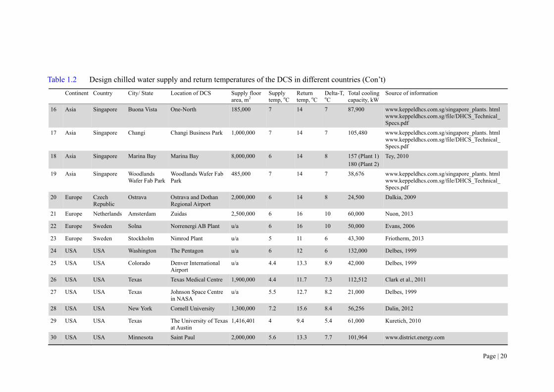
Table 1.2 lists out the design chilled water supply and return temperatures, and the
temperature difference of different DCS projects in different countries. A summary of
the design temperature range in different continents is given in Table 1.3. It can be seen
that the temperature difference in DCS ranges from 5.4-10.5oC and is relatively higher
than that in the conventional chilled water system in buildings, i.e. 5oC. The operating
efficiency of the chilled water system can be increased with an increased temperature
difference due to the reduced pumping requirement caused by a reduced flow rate in the
distribution system.

Page | 19
Table 1.2 Design chilled water supply and return temperatures of the DCS in different countries
Continent Country City/ State Location of DCS Supply floor area, m2
Supply temp, oC
Return temp, oC
Delta-T, oC
Total cooling capacity, kW
Source of information
1 Asia Japan Chiba Chiba Newtown Center 467,000 7 14 7 29,183 www.nt-cnc.co.jp/netu/index3.html
2 Asia Japan Fukuoka Fukuoka Seaside Momochi District
691,812 6 12 6 55,201 www.jdhc.or.jp/area/kyushu/06.html www.fukuoka-es.co.jp/area/momochi.html
3 Asia Japan Kobe Southern District of Sannomiya Station
78,200 7 14 7 11,075 www.ores-dhc.co.jp/system/sannomiya.html
4 Asia Japan Osaka Kinki 238,109 7 14 7 39,000 www.ores-dhc.co.jp/system/konohana.html
5 Asia Japan Osaka Nanko 750,000 6.5 13 6.5 62,233 www.ores-dhc.co.jp/system/nankou.html
6 Asia Japan Osaka Rinku Town 245,634 6 13.5 7.5 23,206 www.ores-dhc.co.jp/system/rinku.html
7 Asia Japan Tokyo Downtown Waterfront District
2,132,953 7 14 7 221,860 www.jdhc.or.jp/area/tokyo/47.html www.tokyo-rinnetu.co.jp/?page_id=11
8 Asia Japan Tokyo Ikebukuro 605,257 5 14 9 71,023 www.jdhc.or.jp/area/tokyo/04.html www.ikenetu.co.jp/area/index.html
9 Asia Japan Yokohama Minato Mirai 21 2,793,900 6 13 7 130,795 www.jdhc.or.jp/area/kanto/01.html www.mm21dhc.co.jp/english/owner/erea_center. php
10 Asia Japan Tokyo Shinjyuku Shin-toshin District
2,222,630 4 12 8 207,444 www.hitachi-ap.com/products/business/chiller_ heater/district/ shinjyuku.html
11 Asia Japan Tokyo Shinjuku South 241,000 7 14 7 36,813 www.jdhc.or.jp/area/tokyo/52.html www.sesdhc.co.jp/dhc/equipment_outline. html
12 Asia Japan Tokyo Shiodome Kita 719,777 4 14.5 10.5 95,973 www.jdhc.or.jp/area/tokyo/63.html www.shiodome-ue.co.jp/index4.html
13 Asia Malaysia Kuala Lumpur Kuala Lumpur City Centre
604,000 4.4 14.4 10 128,000 Majid et al., 2008
14 Asia Malaysia Kuala Lumpur Kuara Lumpur International Airport
605,320 7.5 14.5 7 123,060 Majid et al., 2008
15 Asia Malaysia Perak University Technology Petronas
104,000 6 13 7 48,520 Majid et al., 2008
Page | 20
Table 1.2 Design chilled water supply and return temperatures of the DCS in different countries (Con’t)
Continent Country City/ State Location of DCS Supply floor area, m2
Supply temp, oC
Return temp, oC
Delta-T, oC
Total cooling capacity, kW
Source of information
16 Asia Singapore Buona Vista One-North 185,000 7 14 7 87,900 www.keppeldhcs.com.sg/singapore_plants. html www.keppeldhcs.com.sg/file/DHCS_Technical_ Specs.pdf
17 Asia Singapore Changi Changi Business Park 1,000,000 7 14 7 105,480 www.keppeldhcs.com.sg/singapore_plants. html www.keppeldhcs.com.sg/file/DHCS_Technical_ Specs.pdf
18 Asia Singapore Marina Bay Marina Bay 8,000,000 6 14 8 157 (Plant 1)180 (Plant 2)
Tey, 2010
19 Asia Singapore Woodlands Wafer Fab Park
Woodlands Wafer Fab Park
485,000 7 14 7 38,676 www.keppeldhcs.com.sg/singapore_plants. html www.keppeldhcs.com.sg/file/DHCS_Technical_ Specs.pdf
20 Europe Czech Republic
Ostrava Ostrava and Dothan Regional Airport
2,000,000 6 14 8 24,500 Dalkia, 2009
21 Europe Netherlands Amsterdam Zuidas 2,500,000 6 16 10 60,000 Nuon, 2013
22 Europe Sweden Solna Norrenergi AB Plant u/a 6 16 10 50,000 Evans, 2006
23 Europe Sweden Stockholm Nimrod Plant u/a 5 11 6 43,300 Friotherm, 2013
24 USA USA Washington The Pentagon u/a 6 12 6 132,000 Delbes, 1999
25 USA USA Colorado Denver International Airport
u/a 4.4 13.3 8.9 42,000 Delbes, 1999
26 USA USA Texas Texas Medical Centre 1,900,000 4.4 11.7 7.3 112,512 Clark et al., 2011
27 USA USA Texas Johnson Space Centre in NASA
u/a 5.5 12.7 8.2 21,000 Delbes, 1999
28 USA USA New York Cornell University 1,300,000 7.2 15.6 8.4 56,256 Dalin, 2012
29 USA USA Texas The University of Texas at Austin
1,416,401 4 9.4 5.4 61,000 Kuretich, 2010
30 USA USA Minnesota Saint Paul 2,000,000 5.6 13.3 7.7 101,964 www.district.energy.com

Chapter 1
Page | 21
Table 1.3 Range of design supply and return chilled water temperatures of the DCS in Asia, Europe and the United States
Continents Chilled water temperature, oC
Supply Return Delta-T
Asia (Japan, Singapore and Malaysia) 4-7.5 12-14.5 6-10.5
Europe (Sweden, Netherlands and Czech Republic) 5-6 11-16 6-10
United States 4-7.2 9.4-15.6 5.4-8.9
In 2009, the Energy Market Authority (EMA) of Singapore issued an Energy Service
Supply Code for DCS service providers. Under this code, the operator undertakes to
regulate the chilled water supply temperature within 6ºC ± 0.5ºC and the consumer has
to ensure that the chilled water return temperature should be 14ºC or higher (EMA,
2009).
In Hong Kong, researchers such as Yik et al. (2001b) and Chow et al. (2004b) have
selected 5oC and 12.5oC to be the design chilled water supply and return temperatures
respectively in their research study. These temperatures are typically used for buildings
in Hong Kong and are within the range of chilled water temperatures of the DCS in
other countries. In 2012, the Hong Kong EMSD (2012c) issued a draft technical
guideline for setting up DCS. Under this guideline, chilled water pipes in the
distribution network shall be connected to the plate type heat exchangers installed inside
the user’s premises. The design chilled water supply and return temperatures in the
distribution loop are 5°C (± 1°C) and 13°C. The design chilled water supply and return
temperatures at the building’s chilled water side under normal operating conditions are
6°C (± 1°C) and 14°C. Both the operator and the consumer have the obligations to fulfil
these design conditions to ensure energy efficiency and that all consumers are supplied
with high quality chilled water.
However, there is still no universal standard for determining an optimum chilled water
supply and return temperature and hence the temperature difference for optimizing
energy performance of DCS at low delta-T. Changing this temperature will have a
significant impact on the energy performance of chillers and chilled water pumps as the
COP of chillers and chilled water flow rate in the distribution network are affected.

Chapter 1
Page | 22
This has led to the need to conduct a detailed investigation and find out an optimum
chilled water temperature that can strike a good balance between chiller power and
chilled water pump power to minimize the overall electricity consumption of DCS.
1.5.4 Energy Saving Potentials of P-S and VPF Pumping Systems
For the Hong Kong KTD project, a P-S system was originally proposed in the
consultancy reports (Yik et al. 2001a; Chow et al., 2004a). However, a VPF system was
later adopted during the tendering stage in 2010 (see Table 1.1). VPF system
configuration requires installation of one group of variable speed primary pumps with a
higher pressure head in the chiller plant instead of using one set of primary constant
speed and one set of secondary variable speed pumps in the P-S system. Moreover,
almost all the chillers (except those four with a small cooling capacity) are constant
speed. This may help to save the initial capital cost incurred by variable speed chillers
and additional secondary chilled water pumps for the P-S system.
However, as explained in section 1.4.2 of this chapter, with the advancement in
technology, the efficiency of the primary pump with a lower pressure head can be
designed as high as 85%, which is comparable to the efficiency of pumps with a higher
pressure head and the same design chilled water flow rate. And, the use of variable
chilled water flow chillers in the VPF system does not bring any benefit in energy
consumption as compared to using constant chilled water flow chillers in the P-S
system.
In this regard, VPF systems may not be a good choice for DCS. There has been a lack
of detailed quantitative analysis regarding the energy savings resulting from application
of P-S and VPF systems in the chilled water pumping system of a large scale DCS,
which is similar to the one in the present study. A comparative analysis of the energy
performance of the pumping systems in the P-S and VPF schemes is given in Chapter 4.

Chapter 1
Page | 23
1.6 Financial Analysis
In view of the huge capital investment and the lengthy payback period required by a
large scale infrastructural development like DCS, adoption of measures that can
improve the system’s energy efficiency may increase the capital cost and subsequent
replacement, operating and maintenance costs. The DCS owner may have concerns over
these additional costs. To the system designer, there is always a budgetary constraint in
selecting or designing an optimum set of energy efficiency enhancement measures.
Therefore, to help these parties gain more insights about the real costs and ultimate
energy benefits, a financial analysis of the cost effectiveness of various energy
efficiency enhancement measures is indispensable.
A life cycle cost (LCC) approach is the most widely used method in cost-effectiveness
analysis for comparing the economic viability of various types of energy efficiency
enhancement measures (Master and Ela, 1998; Field and Field, 2009). The technique is
based on discounting, or reducing, all costs to current values or representing them as an
annual cost. The smaller the LCC value, the more worthwhile the option is to be taken
in comparison with other options.
1.7 Research Aim and Objectives
Most research studies have focused on only a few design measures to mitigate the
impacts of low delta-T in the existing chilled water systems in buildings. There is a lack
of comprehensive review and in-depth research on the design of DCS, with an aim to
minimizing the impacts of low delta-T on its energy performance.
As a result, this research is aimed at finding out a cost-optimal design that can enable
the chiller plant and pumping station in a DCS to achieve a satisfactory energy
performance and the minimum long term LCC under the influence of the low delta-T
problems. This aim can be achieved through the following objectives.
i. To construct a hypothetical district model to represent the high-rise buildings in
a commercial district in Hong Kong and design a typical DCS for providing
Chapter 1
Page | 24
chilled water to the district. As the first DCS in Hong Kong is still at a
burgeoning stage, field data about its energy performance, in particular that
related to the impacts of low delta-T, is not yet available. In this regard, a
model-based approach is the most practical and cost effective evaluation method.
Together with a design DCS for the hypothetical district, they provide a vital
simulation environment for this study.
ii. To tailor design mathematical models for a hydraulic distribution network and
all major equipment of a DCS, including constant and variable speed chillers,
variable speed chilled water pumps, heat exchangers and cooling coils of
buildings. These models can act as an effective tool for energy simulation and an
evaluation of the impacts of low delta-T on the DCS’ energy performance.
iii. To propose and evaluate the effectiveness of various energy efficiency
enhancement measures that can mitigate the impacts of low-delta T on the DCS’
energy performance.
In order to achieve these objectives, it is necessary to examine and find out an
optimum design, which is derived from a combination of the following three
energy efficiency enhancement measures:
a. chiller system configuration – this can be done by changing the major
influential design parameters such as the number and cooling capacity of
chillers, and application of constant and variable speed chillers;
b. pumping station – this can be done by analyzing the application of multiple
pumping stations in different locations of the chilled water supply and return
network, and the use of different number of pumps in each pumping station;
and
c. design chilled water supply and return temperatures – this can be done by
conducting a sensitivity analysis of different temperature regimes.

Chapter 1
Page | 25
iv. To devise a cost-optimal design solution that can integrate the various measures
in item (iii), and lead to the lowest LCC and an optimum energy performance
when the DCS is operating under low delta-T conditions.
1.8 Research Methodology
As the development of Hong Kong’s first DCS was still at an early stage when the
present study was conducted, records of its operating energy performance were
unavailable. Therefore, a model-based approach was the only practical and feasible
methodology to be taken. Besides, it is a flexible method that can allow different
scenarios to be studied. To provide a basis for the study, it was necessary to set up a
hypothetical district that could represent the typical urban districts in Hong Kong and a
DCS model had to be designed for this district. The model was first incorporated with
typical design parameters and was taken as the base case. The effectiveness of different
energy efficient measures was then evaluated by modifying the base case model.
Moreover, mathematical models were tailor-made for analyzing the DCS’ performance
under various operating conditions.
Figure 1.9 outlines the approach and methodology adopted for identifying the optimum
design solution for DCS.

Chapter 1
Page | 26
Figure 1.9 Framework of research approach and methodology

Chapter 1
Page | 27
The following is a detailed explanation of each step.
Step 1 – Develop a hypothetical district model
A hypothetical district model was established on the basis of the building
models developed by Yik et al. (2001b). In their study, four building models
comprising a range of combinations of offices, retail shops, restaurants and
hotel guestrooms were formulated to represent the densely populated high-rise
buildings in typical commercial districts in Hong Kong. The hypothetical
district model for the present study was made up of six building zones, each
comprising of a group of these four building models.
Step 2 – Simulate the hourly cooling load profile
Two simulation programs, namely HTB2 (Alexander, 1996) and BECON, (Yik,
1996) were used to predict the cooling loads of the four building models at
different times of the year and the hourly power demand of air conditioning
equipment. The cooling capacity required of the DCS serving the group of
buildings, and the simultaneous hourly cooling loads on the DCS in the year
were determined on this basis.
Step 3 – Develop a baseline DCS model for the hypothetical district
Based on the cooling load data obtained from Step 2, a baseline DCS, named as
“DCSO”, was designed to serve the hypothetical district. This DCS was used as
a reference base for an evaluation of the effectiveness of various energy
efficiency enhancement measures that can further improve the energy
efficiency of the system.
Step 4 – Recommend the energy efficiency enhancement measures for DCSO
To improve the overall energy performance of DCSO under low delta-T
conditions, measures can be taken in the following areas (Figure 1.10).

Chapter 1
Page | 28
Figure 1.10 Three different energy efficiency enhancement measures for DCSO
a. chiller system configuration – this can be done by changing the major
influential design parameters such as the number, cooling capacity and type
(constant or variable speed) of chillers;
b. chilled water supply and return temperatures – this can be done by conducting
a sensitivity analysis of different design chilled water supply and return
temperatures; and
c. pumping station configuration – this can be done by analyzing the application
of multiple pumping stations at different locations of the chilled water supply
and return network, and the use of different number of pumps in each
pumping station.

Chapter 1
Page | 29
Step 5 – Develop mathematical models for the DCS
There are many well-developed mathematical models for air-conditioning
equipment and chilled water systems for application in buildings. They,
however, cannot be applied directly to modelling a DCS. For the present study,
specific mathematical models were developed for simulation of the major DCS
components, including constant and variable speed chillers, variable speed
pumps, heat exchangers, the hydraulic distribution network and the cooling
coils in buildings.
Step 6 – Evaluate the impacts of low delta-T
This baseline DCS and the system and equipment models provided a vital
simulation platform for conducting a comparative analysis of the energy
performance of DCSO with and without the low delta-T syndrome.
Step 7 – Evaluate the effectiveness of the energy efficiency enhancement measures in
three areas (Figure 1.10)
To evaluate the effectiveness of various combinations of measures in these
three areas, DCSO was modified by changing its design parameters. The
objective was to find out the feasible measures that can improve the energy
performance of DCSO.
Step 8 – Determine a cost-optimal design solution
Based on the results of Step 7, many possible design solutions integrated with
different energy efficiency enhancement measures were identified. A simple
heuristic algorithm was developed to select the effective solutions for a more
detailed evaluation of their energy, financial and environmental performances.
For evaluation of the financial viability of these possible solutions, an LCC
model was established and used to find out the ultimate solution, which should
lead to the lowest LCC.

Chapter 1
Page | 30
1.9 Scope and Organization of this Thesis
This thesis is organized into nine chapters, which are grouped under six primary
sections. A graphical representation of the relationship between the chapters is given in
Figure 1.11.
Figure 1.11 Organization of the thesis

Chapter 1
Page | 31
Chapter 2 presents the design of a hypothetical district comprising different
combinations of buildings with a total cooling load of around 200 MW. A district
cooling system, DCSO, was designed to provide centralized chilled water to the
buildings in the district. Three energy efficiency enhancement measures related to
chiller system configuration, pumping station configuration, and chilled water
temperature were proposed. DCSO was treated as a base case for a comparative analysis
of the effectiveness of these three measures.
In Chapter 3, mathematical models were tailor-designed for all the major DCS
equipment such as constant and variable speed chillers, variable speed chilled water
pumps, heat exchangers, a hydraulic distribution network and the building’s cooling
coils. These models were used to simulate the energy performance of DCSO designed
with the energy efficiency enhancement measures mentioned in Chapter 2.
Chapter 4 presents the findings of a comparative analysis of the pumping energy
performance of P-S and VPF systems at low delta-T and the impacts of low delta-T on
the energy performance of DCSO.
In Chapter 5, the effects of changing the chiller system configuration on the energy
performance of DCSO at low delta-T via a study of the key design parameters such as
the number, cooling capacity and type of chillers are evaluated. The aim was to find out
an optimum combination of these parameters, which could improve the energy
performance of DCSO.
Chapter 6 presents the results of an evaluation of the impacts of changing the pumping
station’s configuration on the energy performance of DCSO. The measures included the
use of multiple pumping stations and an unequal number of pumps in each station. In
view of the vast number of pumping station combinations possible for analysis, a
hydraulic gradient evaluation method was adopted to assist a quick assessment and
exploration of those combinations that would be technically feasible. Furthermore, the
energy performance of all these technically feasible combinations was evaluated to
identify an optimum design that would lead to the lowest electricity consumption.

Chapter 1
Page | 32
Chapter 7 gives a comparison of the effects of changing the design chilled water
temperature on the energy performance of DCSO. Different chilled water temperature
regimes were designed and compared to find out an optimum range that could minimize
the overall electricity consumption of DCSO.
In Chapter 8, all the possible design solutions were identified, as a result of combining
the energy efficiency enhancement measures mentioned in Chapters 5, 6 and 7. To
reduce the number of possible solutions, a simple heuristic algorithm was developed. In
addition, an LCC model was established to compare the LCC and understand the
financial viability of these possible solutions. The results could also be used for
determining an ultimate solution that could achieve the least long term total cost of an
ownership and an optimum energy performance.
Chapter 9 concludes this thesis with a summary of the key findings reported in all
preceding chapters, and is followed by some recommendations for further research that
would help to design a more energy efficient DCS for Hong Kong.

Chapter 2
Page | 33
Chapter 2
Development of a Hypothetical District and Energy Efficiency
Enhancement Measures
2.1 Overview
This chapter consists of six sections. Section 2.2 presents the design of a hypothetical
district that was made up of office buildings, commercial complexes and hotels to
represent the commercial districts in Hong Kong. The configuration of a hypothetical
DCS for serving this district is illustrated in Section 2.3. Three energy efficiency
enhancement measures related to chiller system configuration, pumping station
configuration and chilled water temperature are proposed in Sections 2.4, 2.5 and 2.6.
Section 2.7 gives a summary of this chapter.
2.2 Development of a Hypothetical District
2.2.1 Scale of the Hypothetical District
A number of consultancy and research studies (EMSD, 1999; Yik et al., 2001a; Yik et
al., 2001b; EMSD, 2003a; EMSD, 2003b; Chow et al., 2004b; EMSD, 2005) were
conducted to analyze the energy benefits of adopting DCS in Hong Kong and predict
the impacts of using different heat rejection methods for DCS. For example, based on

Chapter 2
Page | 34
the results of energy simulation, Chow et al. (2004b) concluded that once-through direct
seawater cooling scheme using variable flow seawater pumps was the most suitable for
the South East Kowloon Development Project in Hong Kong from an economic point of
view. However, these studies did not address in detail the issue of finding an optimum
scale of DCS so that it could be the most cost effective in terms of initial capital
investment and operating costs.
Lo et al. (2006) carried out a techno-economic analysis for optimization of DCS
application to a large city such as Hong Kong. They studied into adopting DCS as an
alternative to air-cooled air-conditioning systems (AACS) or water-cooled
air-conditioning systems (WACS) in individual buildings in a district. Six hypothetical
district models consisting of different types of premises were established to represent
the district, which had a peak total cooling demand that ranged from 10 MW to 200 MW.
The energy simulation results showed that adoption of direct seawater-cooled DCS
could significantly reduce the annual electricity consumption of the water-side
air-conditioning system. The savings were 20-25% and 9-15% when compared to
equipping individual buildings in a district with their own AACS and WACS
respectively. In that study, a cost model was also established to evaluate the economic
viability of the DCS. The results showed that the energy cost saving of using DCS was
high enough to compensate for the additional capital cost investment in comparison
with AACS or WACS. DCS was found to be the lowest in terms of its annualized unit
cost (AUC), i.e. the present value of life cycle cost per unit cooling output per annum,
thus making it economically favourable.
Moreover, the DCS exhibited the effect of economy of scale. It was also found that the
AUC of energy for producing chilled water decreased as the scale of the DCS increased.
However, this levelled off when the cooling capacity reached 200 MW. On the other
hand, the AUC of a small scale DCS, i.e. less than 20 MW, was found to be not
competitive against individual buildings using WACS. In this regard, in the present
study, the cooling capacity of a DCS was set at 200 MW, which is close to the scale of
the biggest single DCS in Japan - the Shinjuku District Heating and Cooling Centre.
This centre has a cooling capacity of 208 MW for a total service floor area of 2.2
million square meters (EMSD, 2013).

Chapter 2
Page | 35
2.2.2 Types of Building
In Hong Kong, buildings in commercial districts, for example, Central, Wan Chai and
Causeway Bay, are dominated by premises such as offices, retail shops, restaurants and
hotels. For the KTD, the gross floor area of these premises attributes over 70% of that
of the entire project (Chow et al., 2004a). Hence, these premises were used to represent
the commercial district in this study. In 2001, Yik et al. (2001a) studied 23
office/commercial buildings and 16 hotels, and developed four different building
models with different combinations of these premises. These four models are denoted as
buildings A to D in this study (see Table 2.1). The survey data that Yik et al. (2001a)
collected also provided information for the patterns of occupancy, appliance loads and
lighting loads to be used in the current simulation study.
Table 2.1 Key characteristics of the four building models
Building A represents an office-only building, whereas buildings B and C represent
building complexes comprising a combination of different functional areas such as
single-tenanted offices, multi-tenanted offices, retail shops and restaurants. The fourth
model, i.e. building D, represents a hotel block comprising guestrooms and commercial
units. In Hong Kong, the ground floors of commercial buildings or hotels are often used
as entrance lobby and some commercial buildings may consist of communal podiums
Unit Building A Building B Building C Building D
Type of building Office Commercial complex
Commercial complex
Hotel
No. of storey 40 32 17 26
Gross floor area:
Office m2 91,000 54,600 31,850 0
Retail m2 0 13,650 4,550 22,750
Restaurant m2 0 4,550 2,275 6,825
Guestroom m2 0 0 0 29,575
Total m2 91,000 72,800 38,675 59,150
On each floor:
Floor-to-floor height m 3.2 3.5 3.5 3.5
Construction floor area m2 2,500 2,500 2,500 2,500
Air-conditioned area m2 2,275 2,275 2,275 2,275
Operating period:
Weekday 0800 - 2000 0600 - 2300 0600 - 2300 0000 - 2400
Saturday 0800 - 1600 0600 - 2300 0600 - 2300 0000 - 2400
Sunday Off 0600 - 2300 0600 - 2300 0000 - 2400

Chapter 2
Page | 36
above the ground floor. For simplicity, entrance lobbies and podiums were not included
in the design of the four building models in this study. Figure 2.1 shows the typical floor
plans and elevations of these building models and Table 2.2 shows the mixes of the five
functional areas in buildings A to D.
Figure 2.1 Typical layout and sections of the four building models
Table 2.2 Number of storeys occupied by the five functional areas in the four building models
Model building Building A Building B Building C Building D
Type Office Commercial complex
Commercial complex
Hotel
Office (single-tenanted) 40 0 0 0
Office (multi-tenanted) 0 24 14 0
Retail 0 6 2 10
Restaurant 0 2 1 3
Guestroom 0 0 0 13
Total no. of storey 40 32 17 26

Chapter 2
Page | 37
2.2.3 Air-Conditioning System Design
2.2.3.1 Offices
A typical office building in Hong Kong adopts either a primary air fan-coil system or a
variable air volume (VAV) system, depending on the specific usage characteristics of
the individual air-conditioned space. For either system, there is typically a central
primary air system supplying treated fresh air to the air-conditioned spaces.
There are two major types of office buildings in Hong Kong: multi-tenanted and
single-tenanted office buildings. Fan coil units (FCU) are widely used in multi-tenanted
office buildings, which may be leased or sold. The system design is relatively simple in
comparison with other air-side systems. They provide more flexibility in partitioning
and leasing to different tenants on the same floor.
VAV systems, which are more common among single-tenanted offices, are more energy
efficient as compared to constant air volume (CAV) systems (Yang and Ting, 2000; Wei
and Zmeureanu, 2009). VAV systems are increasingly equipped with variable speed fans
for the much greater fan energy saving achievable. Their energy performance can be
further improved through the use of an economizer cycle, which eliminates or reduces
refrigeration cooling by utilizing the free cooling capacity of the ambient environment.
This, however, is rare in Hong Kong due to the large outdoor air intake and exhaust
ducts and grilles or louvers required. In a VAV system, the air handling unit (AHU)
treats and distributes conditioning air at a constant temperature to multiple VAV boxes
placed above the false ceiling of the air-conditioned spaces. Control of air distribution is
accomplished through the pressure independent VAV boxes that control the amount of
supply air to the space according to the temperature of the space fed back by the indoor
temperature sensor. The speed of the supply air fan inside the AHU will be controlled to
regulate the flow rate of supply air to the air-conditioned spaces.
To ensure that the hypothetical building models can well represent the situation of Hong
Kong, both multi-tenanted and single-tenanted offices were covered in this study. A

Chapter 2
Page | 38
VAV system was designed for the single-tenanted offices in building A, while a FCU
system was designed for the multi-tenanted offices in buildings B and C.
2.2.3.2 Restaurants and Retail Shops
CAV systems were designed to serve locations where a high rate of air infiltration
would arise due to frequent movement of people. A constant high air flow rate is
desirable to lower the space temperature and humidity when there is an in-rush of warm
and humid air. The control of zone temperature is accomplished by varying the supply
air temperature in response to the feedback signal from the indoor temperature sensor.
2.2.3.3 Hotel Guestrooms
Primary air fan coil systems are the most typical design for guestrooms in hotels. Their
arrangement is similar to the design used for the multi-tenanted offices. A thermostat
with a three-speed fan switch is provided for each FCU to control the temperature and
air flow rate. The system type and design criteria of the air-conditioning system for an
individual area are given in Table 2.3.
Table 2.3 Design criteria for the air-conditioning system in the five functional areas
Functional area Air-side system Design condition (1) Fresh air flow rate (2)
Summer Winter
Office (multi-tenanted) PAU + FCU 23oC DB 22oC DB 10 l/s/person
Office (single-tenanted) AHU + PAU (VAV) 23oC DB 22oC DB 10 l/s/person
Restaurant AHU + PAU (CAV) 22oC DB 22oC DB 10 l/s/person
Retail shop AHU + PAU (CAV) 22oC DB 24oC DB 1 l/s/m2
Hotel guestroom PAU + FCU 22oC DB 24oC DB 15 l/s/room
Remarks:
1. From EMSD, 2012c. 2. From ASHRAE, 2001.
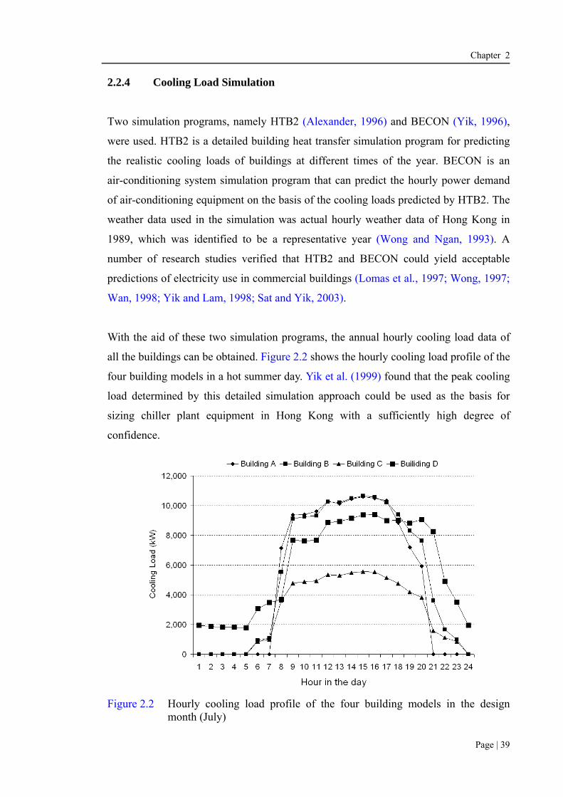
Chapter 2
Page | 39
2.2.4 Cooling Load Simulation
Two simulation programs, namely HTB2 (Alexander, 1996) and BECON (Yik, 1996),
were used. HTB2 is a detailed building heat transfer simulation program for predicting
the realistic cooling loads of buildings at different times of the year. BECON is an
air-conditioning system simulation program that can predict the hourly power demand
of air-conditioning equipment on the basis of the cooling loads predicted by HTB2. The
weather data used in the simulation was actual hourly weather data of Hong Kong in
1989, which was identified to be a representative year (Wong and Ngan, 1993). A
number of research studies verified that HTB2 and BECON could yield acceptable
predictions of electricity use in commercial buildings (Lomas et al., 1997; Wong, 1997;
Wan, 1998; Yik and Lam, 1998; Sat and Yik, 2003).
With the aid of these two simulation programs, the annual hourly cooling load data of
all the buildings can be obtained. Figure 2.2 shows the hourly cooling load profile of the
four building models in a hot summer day. Yik et al. (1999) found that the peak cooling
load determined by this detailed simulation approach could be used as the basis for
sizing chiller plant equipment in Hong Kong with a sufficiently high degree of
confidence.
Figure 2.2 Hourly cooling load profile of the four building models in the design
month (July)
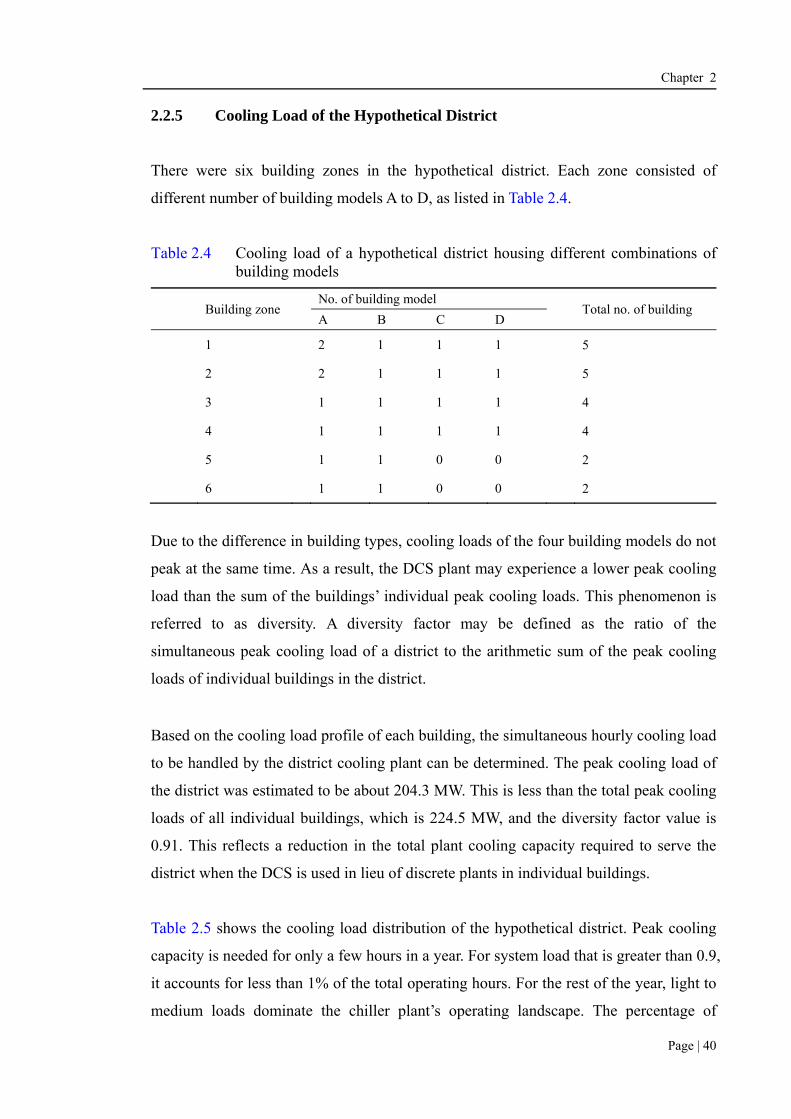
Chapter 2
Page | 40
2.2.5 Cooling Load of the Hypothetical District
There were six building zones in the hypothetical district. Each zone consisted of
different number of building models A to D, as listed in Table 2.4.
Table 2.4 Cooling load of a hypothetical district housing different combinations of building models
Building zone
No. of building model Total no. of building
A B C D
1 2 1 1 1 5
2 2 1 1 1 5
3 1 1 1 1 4
4 1 1 1 1 4
5 1 1 0 0 2
6 1 1 0 0 2
Due to the difference in building types, cooling loads of the four building models do not
peak at the same time. As a result, the DCS plant may experience a lower peak cooling
load than the sum of the buildings’ individual peak cooling loads. This phenomenon is
referred to as diversity. A diversity factor may be defined as the ratio of the
simultaneous peak cooling load of a district to the arithmetic sum of the peak cooling
loads of individual buildings in the district.
Based on the cooling load profile of each building, the simultaneous hourly cooling load
to be handled by the district cooling plant can be determined. The peak cooling load of
the district was estimated to be about 204.3 MW. This is less than the total peak cooling
loads of all individual buildings, which is 224.5 MW, and the diversity factor value is
0.91. This reflects a reduction in the total plant cooling capacity required to serve the
district when the DCS is used in lieu of discrete plants in individual buildings.
Table 2.5 shows the cooling load distribution of the hypothetical district. Peak cooling
capacity is needed for only a few hours in a year. For system load that is greater than 0.9,
it accounts for less than 1% of the total operating hours. For the rest of the year, light to
medium loads dominate the chiller plant’s operating landscape. The percentage of

Chapter 2
Page | 41
system load that is less than 50% accounts for 77% of the total operating hours. This
suggests that the chiller system needed to be operated under part load conditions for
most of the time.
Table 2.5 Cooling load distribution of the hypothetical district
% of design cooling load % of operating hour
<10 34
10 < L≤ 20 12
20 < L≤ 30 13
30 < L≤ 40 12
40 < L≤ 50 6
50 < L≤ 60 4
60 < L≤ 70 5
70 < L≤ 80 6
80 < L≤ 90 7
90 < L≤ 100 1
2.3 Design of a Baseline DCS
Figure 2.3 shows a schematic diagram of the basic design of a DCS for the hypothetical
district.
Figure 2.3 Schematic diagram of DCSO designed for the hypothetical district

Chapter 2
Page | 42
This DCS, denoted as DCSO, consisted of a production loop, a distribution loop and
building loops. It adopted a constant primary-variable secondary scheme for chilled
water distribution instead of a variable primary flow pumping scheme, because the latter
is not an energy efficient chilled water pumping system in DCS. A detailed comparative
analysis of the energy performance of the two schemes that justifies this selection is
given in Chapter 4.
The chilled water distribution system comprises constant speed primary pumps in the
production loop and variable speed secondary pumps in the distribution loop. A constant
chilled water flow rate is maintained in the production loop which prevents the
temperature from dropping too low to impair the evaporator and avoid frequent
shutdown of chillers. The variable flow in the distribution loop can maximize the
difference between the supply and return chilled water temperatures, and minimize
pumping system energy in the distribution loop. A decoupler by-pass pipe hydraulically
decouples the production and distribution pumps so that they can each operate at a
different flow rate independent of each other.
2.3.1 Production Loop
2.3.1.1 Heat rejection method is a crucial factor that affects the energy efficiency of
chillers. WACS are widely adopted in DCS as they are more energy efficient
than AACS. In a WACS, seawater or fresh water may be used as a cooling
medium for removal of the rejected heat from the condensers of the DCS’
chillers. In the absence of major rivers in Hong Kong, only those districts that
are situated near the harbour can adopt seawater cooling. A study conducted
by Yik et al. (2001b) showed that direct seawater-cooled system was the most
energy efficient (COP = 5.2) in comparison with fresh water-cooled systems
with cooling towers and indirect seawater-cooled systems (COP = 4.7).
Figure 2.4 shows a direct seawater-cooled system, which uses seawater to
absorb the rejected heat from the chiller condensers in a DCS. This system is
applied in large centralized air-conditioning installations where sufficient
cooling water is available, such as the areas along the seafront of Victoria

Chapter 2
Page | 43
Harbour. In Hong Kong, over 25 million cubic meters of seawater is used for
cooling purpose everyday (Ma et al., 1998).
Figure 2.4 Schematic of the direct seawater cooling system of the DCS
For a direct seawater cooling scheme, the temperature of the intake seawater
affects the chiller’s performance significantly. Chow et al. (2004a) showed
that the COP of a typical centrifugal chiller with a large cooling capacity
increased by about 20% when the temperature of cooling water at the
condenser inlet decreased from 30oC to 20oC (Figure 2.5). Moreover, a
chiller’s COP increased significantly with its design capacity, to up to 5.5
MW (or 1,500 RT). There was a significant increase in the COP if the
chiller’s cooling capacity was above 1,500 RT. Beyond this capacity, no
significant increase in COP could be observed. They remarked that the
largest R-134a type of vapour-compression chiller currently available on the
market would be 22.1 MW (6,000 RT).
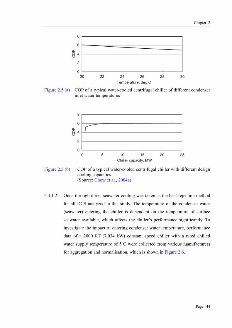
Chapter 2
Page | 44
Figure 2.5 (a) COP of a typical water-cooled centrifugal chiller of different condenser
inlet water temperatures
Figure 2.5 (b) COP of a typical water-cooled centrifugal chiller with different design
cooling capacities (Source: Chow et al., 2004a)
2.3.1.2 Once-through direct seawater cooling was taken as the heat rejection method
for all DCS analyzed in this study. The temperature of the condenser water
(seawater) entering the chiller is dependent on the temperature of surface
seawater available, which affects the chiller’s performance significantly. To
investigate the impact of entering condenser water temperature, performance
data of a 2000 RT (7,034 kW) constant speed chiller with a rated chilled
water supply temperature of 5oC were collected from various manufacturers
for aggregation and normalisation, which is shown in Figure 2.6.

Chapter 2
Page | 45
Figure 2.6 Part load performance of a 2,000 RT (7,034 kW) constant speed chiller
The COP of the chiller with a condenser water entering temperature of 20oC
is about 9% higher than that of a chiller with a condenser water temperature
of 25oC. Similarly, when the temperature is 25oC, the COP of the chiller is
also about 9% higher than that with a condenser water temperature of 30oC.
Table 2.6 shows the statistics of the annual seawater temperatures generated
by the model embedded in BECON for prediction of the year round seawater
temperature. Periods in which the seawater temperature is below 25oC occupy
52% of the total operating hours in a year. This illustrates the key advantage
of using direct seawater cooling for heat rejection, as chillers can run at a
higher COP at almost all times throughout the year.

Chapter 2
Page | 46
Table 2.6 Distribution frequency of seawater temperature in a year (Yik,
1996)
Seawater temperature, oC % of occurrence in a year
≤16 0
16 < Tcon≤ 17 9
17 < Tcon ≤ 18 6
18 < Tcon ≤ 19 4
19 < Tcon ≤ 20 5
20 < Tcon ≤ 21 5
21 < Tcon ≤ 22 4
22 < Tcon ≤ 23 5
23 < Tcon ≤ 24 6
24 < Tcon ≤ 25 8
25 < Tcon ≤ 26 12
26 < Tcon ≤ 27 16
27 < Tcon ≤ 28 20
2.3.1.3 Besides the cooling load profile, there are many factors to consider in
designing the configuration of a chiller system. For example, a large number
of combinations and mixes of chiller types and capacities may be considered
but evaluating the performance of each of them to inform selection of the
optimum one is very time consuming.
A simple approach to take is to use equally-sized chillers for a
multiple-chiller system and pump, which will make it much easier to
implement optimized control strategies (e.g. chiller sequencing controls) and
provide greater flexibility for operation and maintenance.
In this study, a chiller plant with multiple, equally-sized and constant speed
centrifugal chillers was first designed to serve as the base case for comparison
with different design options (as will be described in the following chapters).
2.3.1.4 According to the information given by the manufacturers, the maximum
cooling capacity of centrifugal seawater-cooled chillers that are currently
available on the market is about 6,000 RT (21,102 kW). It is a normal practice
to reserve about 10% as a spare cooling capacity for contingency purposes
(Yu, 2001). Based on this consideration, the chiller plant taken as the base

Chapter 2
Page | 47
case in this study was designed to consist of 10 x 6,000 RT (21,102 kW)
chillers to meet the peak load of the hypothetical district.
2.3.1.5 Each chiller is equipped with a dedicated primary chilled water pump and
seawater pump. All are interlocked with one another, i.e. the three would be
switched on and off at the same time. The primary chilled water pump and
seawater pump are constant speed and constant flow pumps.
2.3.1.6 To comply with the EMSD’s technical guidelines for DCS (EMSD, 2012c),
the DCS taken as the base case in this study was designed to supply chilled
water at the temperature of 5oC. The temperature of the return chilled water
was taken as 12oC. The design temperatures of the supply and return chilled
water within the building loop were 7°C and 14°C respectively.
2.3.2 Distribution Loop
2.3.2.1 A pumping station with 10 variable speed pumps was designed downstream
of the chiller plant to circulate chilled water between the DCS and the
buildings.
2.3.2.2 The distribution loop is hydraulically de-coupled from the production loop by
the decoupler bypass pipe between the two loops. All secondary pumps in the
distribution loop are variable speed and variable flow pumps.
2.3.2.3 The diameter of the main chilled water supply and return pipes is about 1,500
mm, based on the following distribution pipe sizing criteria.
i. Pressure drop ranges from 220 to 400 Pa per unit length (Yik et al.,
2001a ; ASHRAE, 2009).
ii. A velocity limit of 1.2 m/s is designed for 50mm pipe and smaller. A
higher velocity of up to 3 m/s (ASHRAE, 2009) was designed for pipes
immediately downstream of the secondary pump so as to ensure that pipe
size would not exceed 1.5 m. Since the pipes are buried underground,

Chapter 2
Page | 48
noise generated as a result of high velocity flow should not be a problem
(Yik et al., 2001a).
iii. The difference between the chilled water supply and return temperature
of the system was designed to be 7oC (Yik et al, 2001a).
2.3.2.4 The total design pipe run of the distribution network is 2,500 km, which is
close to the pipe run in the Kai Tak Development DCS project.
2.3.2.5 CO and PS1-0 denote the base chiller system and pumping station
configuration, respectively. Their details are shown in Table 2.7.
Table 2.7 Design parameters of CO and PS1-0 in DCSO
Chiller system configuration CO
a. Direct seawater-cooled chiller
Type Constant speed
Rated cooling capacity per chiller, kW/RT 21,102 / 6,000
Total no. 10
Rated compressor power, kW 3,419
COP at full load 6.17
Integrated part load value 6.57
Chilled water supply/return temp., oC 5 / 12
Chilled water flow rate, l/s 718
Condenser water entering/leaving temp., oC 29.4 / 35.4
Condenser water flow rate, l/s 973
b. Primary chilled water pump
Total no. 10
Rated flow rate, l/s 718
Pump head, m 16.8
Rated power, kW 164.4
c. Seawater pump
Total no. 10
Rated flow rate, l/s 973
Pump head, m 16.8
Rated power, kW 223.3
Pumping station configuration PS1-0
d. Secondary chilled water pump
Total no. 10
Rated flow rate, l/s 718
Pump head, m 56.9
Rated power, kW 576.0

Chapter 2
Page | 49
2.3.3 Building Loop
2.3.3.1 An energy transfer station is the interface between the building’s cooling
system and the DCS. Each station consists of heat exchangers, isolation and
control valves, controllers, measurement equipment and energy meters. The
building’s chilled water is cooled to the design supply temperature by the heat
exchanger with chilled water of the distribution loop flowing at the other side.
The energy transfer station is located at the perimeters of the building to
ensure ease of installation and operation and maintenance. Only one energy
transfer station will be provided for each building.
2.3.3.2 Heat exchangers are the key components that separate the building’s chilled
water network from the DCS’ distribution network and facilitate heat transfer
from the former to the latter. It is vital to minimize the log mean temperature
difference of the heat exchanger, which requires the use of a close
temperature approach, i.e. within 1°C (EMSD, 2012b). Plate type heat
exchanger is the only type of heat exchanger that can serve this purpose
(Skagestad and Mildenstein, 1999).
2.3.3.3 Each building in the building loop has its own variable speed pumps to
circulate chilled water through the air-side equipment, i.e. FCU and AHU.
Two-way control valves are used in the air-side equipment to modulate the
chilled water flow rate according to the cooling loads on them. At light load,
the valves are closed (partially or fully), resulting in a pressure rise in the
building loop. A differential pressure sensor measures the pressure rise and
this signal is transmitted to the pump speed controller which alters the speed
and hence the chilled water flow rate of the variable speed pumps.
2.4 Design of Energy Enhancement Measure - Chiller System Configuration
The energy performance of a chiller plant can be affected by varying the major
influential system parameters, such as the number, cooling capacity and type of chillers.
This section reviews the impacts of varying each parameter to inform selection of the

Chapter 2
Page | 50
range of these parameters to be considered in the attempt to find out an optimum chiller
system configuration.
2.4.1 Varying the Number of Chiller
Lee and Lee (2007) pointed out that most chillers in commercial buildings had an
optimum operating point that corresponds to the peak energy efficiency, which would
occur at a specific part load ratio. This optimum operating point of typical chillers is
about 80% of the maximum capacity (Trane, 1989; Lee and Lee, 2007). Hence, running
more chillers than the minimum number that can marginally meet the load may reduce
the energy use of the chillers. On the other hand, other factors also need to be
considered, such as spatial requirement, capital cost investment and energy consumption
of other associated equipment, including the chilled and condenser water pumps. More
chillers in operation means that more energy will be consumed by the pumps because
the chilled water pump and the seawater pump are interlocked with the chiller, and will
also be operated whenever their associated chiller is run. Whether the energy
consumption of the extra pumps may be fully offset by the energy saving due to
operating those chillers needs to be evaluated in detail when an optimized sequencing
control strategy is formulated.
No concrete guidelines can be found in the open literature for determining the optimum
number of chillers for a DCS. This deserves further exploration. Reference was made to
the DCS plant in Japan’s Shinjyuku Shin-toshin, which has more or less the same design
cooling capacity as the DCS for the hypothetical district in this study. This Japanese
chiller plant consists of 12 turbo and absorption chillers, including 3 x 10,000 RT
(35,170 kW), 2 x 7,000 RT (24,619 kW), 1 x 4,000 RT (14,068 kW), 1 x 2,870 RT
(10,094 kW), 1 x 2,000 RT (7,034 kW), 2 x 2,065 RT (7,263 kW) and 2 x 1,000 RT
(3,517 kW) chillers. The total installed cooling capacity is 59,000 RT (208 MW). To
avoid complicating the present study, the maximum number of chillers was set to be 15.
2.4.2 Unequally-Sized Chillers
It is a common practice to use equally-sized chillers in designing a chiller system

Chapter 2
Page | 51
(Mcquay International, 2001; Lee and Lee, 2007). This has merits because pumps or
cooling towers are of the same size and are interchangeable, and these are more flexible
to operate and maintain. On the other hand, Landman (1996) and Chan and Yu (2004)
advocated the use of unequally-sized chillers for a chiller plant, as this could prolong
their operation at near full load and reduce electricity consumption of the chiller plant. It
is because unequally-sized chillers allow selection of the most suitable combination of
chillers, which can match more closely the cooling load demand at different operational
periods and achieve the best energy performance.
Therefore, multiple chillers of unequal sizes were considered in this study to see
whether they could help alleviate the adverse impacts of the low delta-T problem.
Traditionally, this can be accomplished by using the rule of thumb, i.e. the size of the
small chiller is one-third or two-thirds of the size of the largest chiller in a plant. Given
that the largest cooling capacity of available direct seawater-cooled chiller is 6,000 RT,
which is also the largest chiller designed for DCS on the commercial market, the chiller
plant in the present hypothetical DCS model was thus designed with three different
sizes: 2,000 RT, 4,000 RT and 6,000 RT. Within the limit of 15 chillers at maximum, the
combinations of chillers are: 5 x 6,000 RT, 5 x 4,000 RT and 5 x 2,000 RT, which
together would provide a total of 60,000 RT (about 210 MW) (Hitachi Appliance Inc.,
2013). This allows flexibility for running different combinations of chillers to meet the
variable load, in particular, during low load conditions.
2.4.3 Variable Speed Chillers
Over the last two decades, the cost of variable speed drives has come down significantly
due to advances in technology and expansion of market size. This technology has also
been applied to chillers. Qureshi and Tassou (1996) conducted a review of the use of
variable speed chiller, and confirmed that variable speed drives had been applied
successfully to perform capacity modulation for chiller compressors. The variable speed
chillers bring about superior part load efficiency, as compared to chillers using multiple
constant speed compressors with cycling control.
As degrading delta-T occurs most often when the cooling load drops to about two-thirds

Chapter 2
Page | 52
to one-half of the design cooling load (Taylor, 2002a), variable speed chillers were
adopted in this study to assess their effectiveness in mitigating the impacts of low
delta-T on the electricity consumption of the chiller plant.
2.4.4 Chiller System Configuration
The base case chiller system configuration, CO, consisted of 10 x 6,000 RT (21,102 kW)
constant speed chillers. With reference to the three design parameters described above,
five additional chiller system configurations, denoted as CA, CB, CC, CD and CE, were
formed, as summarized in Table 2.8. Their total installed cooling capacities still
remained the same as that of CO, i.e. 60,000 RT (21,1020 kW). The effectiveness in
enhancing the energy performance of DCSO at low delta-T, by replacing CO with one of
these chiller system configurations is evaluated in this study. However, the same design
of chilled water distribution system, including the number of pumping stations and the
chilled water temperatures, was applied to all these alternative chiller plants.
Table 2.8 Design parameters of chiller system configurations CO, CA, CB, CC, CD and
CE
Chiller system configuration
CO CA CB CC CD CE
No. of chiller 10 10 15 15 15 15
Size Equal Equal Equal Unequal Equal Unequal
Cooling capacity 10 x 6,000 RT
10 x 6,000 RT
15 x 4,000 RT
5 x 2,000 RT5 x 4,000 RT5 x 6,000 RT
15 x 4,000 RT
5 x 2,000 RT5 x 4,000 RT5 x 6,000 RT
Type Constant speed
Variable speed
Constant speed
Constant speed
Variable speed
Variable speed
The design details of the chillers and the associated primary chilled water pumps and
seawater pumps in these six chiller system configurations, including those of the base
case, are summarized in Table 2.9. A detailed evaluation of their effectiveness in
improving the energy performance over that of DCSO at low delta-T is presented in
Chapter 5.

Page | 53
Table 2.9 Design details of chiller system configurations CO, CA, CB, CC, CD and CE
Chiller system configuration CO CA CB CC CD CE
1. Seawater-cooled chiller
Type Constant speed
Variable speed
Constant speed
Constant speed
Constant speed
Constant speed
Variable speed
Variable speed
Variable speed
Variable speed
Rated cooling capacity per chiller kW (RT)
21,096 (6,000)
21,096 (6,000)
14,064 (4,000)
7,032 (2,000)
16,174 (4,000)
21,096 (6,000)
14,064 (4,000)
7,032 (2,000)
16,174 (4,000)
21,096 (6,000)
Total no. 10 10 15 5 5 5 15 5 5 5 Rated compressor power,
kW 3,419 3,419 2,279 1,140 2,279 3,419 2,279 1,140 2,279 3,419
COP at full load 6.17 6.17 6.17 6.17 6.17 6.17 6.17 6.17 6.17 6.17 Integrated part load value 6.57 9.76 6.57 6.57 6.57 6.57 9.76 9.76 9.76 9.76 Chilled water supply/return
temp, oC 5/12 5/12 5/12 5/12 5/12 5/12 5/12 5/12 5/12 5/12
Chilled water flow rate, l/s 718 718 478 239 478 718 478 239 478 718 Condenser water entering/
leaving temp, oC 29.4/35.4 29.4/35.4 29.4/35.4 29.4/35.4 29.4/35.4 29.4/35.4 29.4/35.4 29.4/35.4 29.4/35.4 29.4/35.4
Condenser water flow rate, l/s 973 973 649 324 649 973 649 324 649 973
2. Primary chilled water pump Total no. 10 10 15 5 5 5 15 5 5 5 Rated flow rate, l/s 718 718 478 239 478 718 478 239 478 718 Pump head, m 16.8 16.8 16.8 16.8 16.8 16.8 16.8 16.8 16.8 16.8 Rated power, kW 164.4 164.4 109.6 56.9 109.6 164.4 109.6 56.9 109.6 164.4
3. Seawater pump Total no. 10 10 15 5 5 5 15 5 5 5 Rated flow rate, l/s 973 973 649 324 649 973 649 324 649 973 Pump head, m 16.8 16.8 16.8 16.8 16.8 16.8 16.8 16.8 16.8 16.8 Rated power, kW 223.3 223.3 149.1 75.3 149.1 223.3 149.1 75.3 149.1 223.3

Chapter 2
Page | 54
2.5 Design of Energy Enhancement Measure - Pumping Station Configuration
In the base case DCSO, only one main pumping station, PS1-0, was located immediately
downstream of the chiller plant. Ten identical variable speed distribution pumps were
designed to simplify maintenance and provide interchangeability of parts.
However, a single pumping station designed for a large district may not be the most
cost-effective design. It is because the design pump head and flow rate are very large so
as to ensure that the chilled water can be distributed to the far end of the district. Under
such circumstances, the building near the pumping station will be over-pressurized. The
pressure is much more than that required in these buildings for overcoming the internal
piping and cooling coil losses. Pressure reducing valves or other energy consuming
mechanical devices have to be installed to prevent over-pressurizing the buildings,
hence making the pumping station not energy efficient. Moreover, there is a large
variation of distribution friction among the buildings in the district. Balance valves have
to be installed to overcome this problem.
Hence, two design initiatives were investigated in this study to optimize the energy
performance of the pumping station. These include the use of:
i. multiple pumping stations – In addition to the main pumping station, additional
booster pumping stations were adopted at different locations along the main chilled
water supply or return pipes of the distribution loop to assist circulation of chilled
water. This can help reduce the pressure head, and hence the power demand of the
main station, while those pumping stations downstream will only need to handle a
smaller chilled water flow rate, which will also help reduce the pumping energy use;
and
ii. multiple pumps in each pumping station – To further optimize the design of the
pumping stations(s), different number of pumps for each station will be explored.
For simplicity, however, this number was limited to 5, 10 or 15.

Chapter 2
Page | 55
2.5.1 Multiple pumping stations
As shown in Figure 2.7, excluding that of the main pumping station, a total of 11
locations along the main chilled water supply or return pipes were identified to be
possible sites for the booster pumping stations for distributing chilled water to all the
buildings and returning it to the central plant.
Figure 2.7 Potential locations for pumping stations
As an example, for the case with two pumping stations in the distribution loop, one
main pumping station must be located before the connection to the first served building,
and one booster pumping station may be at any one of the 11 locations. Therefore, there
are 11 possible combinations of location for these two pumping stations. Similar
arrangement can be made in designing three, four, five or six pumping stations.
According to the calculation in Table 2.10, there were 55, 165, 330 and 462 possible
combinations of locations for placing three, four, five and six pumping stations in the
distribution loop. As a result, there were a total of 1,024 possible combinations for cases
with one to six pumping stations.

Chapter 2
Page | 56
Table 2.10 Total number of combinations of pumping stations (PS)
No. of PS
Possible combination of PS at chilled water supply and/or return sides
No. of combination Total no. of combination
1 Main PS 1 1
2 Main PS plus
1 PS at the supply side 5 (= 5C1) 11
1 PS at the return side 6 (= 6C1)
3 Main PS plus
2 PS at the supply side 10 (= 5C2) 55
2 PS at the return side 15 (= 6C2)
1 PS at the supply and 1 PS at the return side
30 (= 5C1 x 6C1)
4 Main PS plus
3 PS at the supply side 10 (= 5C3) 165
3 PS at the return side 20 (= 6C3)
1 PS at the supply and 2 PS at the return side
75 (= 5C1 x 6C2)
2 PS at the supply and 1 PS at the return side
60 (= 5C2 x 6C1)
5 Main PS plus
4 PS at the supply side 5 (= 5C4) 330
4 PS at the return side 15 (= 6C4)
1 PS at the supply and 3 PS at the return side
100(= 5C1 x 6C3)
3 PS at the supply and 1 PS at the return side
60 (= 5C3 x 6C1)
2 PS at the supply and 2 PS at the return side
150 (= 5C2 x 6C2)
6 Main PS plus
5 PS at the supply side 1 (= 5C5) 462
5 PS at the return side 6 (= 6C5)
1 PS at the supply and 4 PS at the return side
75 (= 5C1 x 6C4)
4 PS at the supply and 1 PS at the return side
30 (= 5C4 x 6C1)
3 PS at the supply and 2 PS at the return side
150 (= 5C3 x 6C2)
2 PS at the supply and 3 PS at the return side
200 (= 5C2 x 6C3)
Total 1,024

Chapter 2
Page | 57
2.5.2 Multiple pumps in each pumping station
Additionally, the number of pumps in each pumping station may be 5, 10 or 15. Taking
the design shown in Figure 2.8 as an example, it is one of the combinations using three
pumping stations in a distribution loop. It consists of one main pumping station at
location PS1,s and two booster pumping stations at locations PS3,s and PS2,r. Figure 2.8 (a)
shows a design with the same number of pumps in all three stations, and Figure 2.8 (b)
represents an arrangement of different number of pumps in each station.
Figure 2.8 (a) An example of a combination of three pumping stations with the same number of pumps in each station

Chapter 2
Page | 58
Figure 2.8 (b) An example of a combination of three pumping stations with different number of pumps in each station
Using this approach, a total of 27 (i.e. = 33) “arrangements” based on the variation in
pump number can be identified for this particular three-pumping station combination, as
shown in Table 2.11. In this chapter, the phrase “pumping station arrangement”
specifically refers to the grouping of pumping station based on the number of pumps.
Table 2.11 An example showing the different arrangements based on the number of pumps, i.e. with 5, 10 or 15 pumps in each pumping station
Arrangement No. of pump in each pumping station
PS1,s PS3,s PS2,r
1 5 5 5
27 arrangements
2 5 5 10
3 5 5 15
4 5 10 5
5 5 10 10
6 5 10 15
27 15 15 15

Chapter 2
Page | 59
As shown in Table 2.10, there are 55 combinations of using three pumping stations.
Hence, there are 1,485 (= 27 arrangements x 55 combinations) pumping station
arrangements that are using three pumping stations.
The above principle was applied to determine the total number of pumping station
arrangement for using Nps number of pumping stations. For a chilled water distribution
network designed with Nps number of pumping stations, there are Ncomb number of
combinations. For each combination of Nps number of pumping stations, there are 3Nps
number of pumping station arrangements. Hence, the total number of pumping station
arrangements of using Nps number of pumping stations that have Ncomb number of
combination is Ncomb x 3Nps.
As shown in Table 2.10, there are 1, 11, 55, 165, 330 and 462 combinations of one, two,
three, four, five and six pumping stations respectively. The number of pumping station
arrangement for each combination of one, two, three, four, five and six pumping
stations would be 3 (=31), 9 (=32), 27 (=33), 81 (=34), 243 (=35) and 729 (=36)
respectively.
Hence, this led to 3 (= 1 x 3) , 99 (= 11 x 9), 1,485 (= 55 x 27), 13,365 (= 165 x 81), 80,
190 (= 330 x 243) and 336,798 (= 462 x 729) arrangements that used one, two, three,
four, five and six pumping stations.
There are a total of 431,940 “arrangements” (= 3 + 99 + 1,485 + 13,365 +80,190 +
336,798).
A detailed evaluation of the effectiveness of these pumping station arrangements for
improving the energy performance of DCSO is presented in Chapter 6.

Chapter 2
Page | 60
2.6 Design of Energy Enhancement Measure - Chilled Water Supply and
Return Temperatures
In a chiller plant, changes in the design chilled water supply and return temperatures
will affect the energy performance of the chiller, secondary chilled water pumps,
seawater pumps and heat losses, which are discussed as follows.
For a chiller, its energy performance, typically gauged by its COP, will increase by
raising the design chilled water supply temperature. A higher design chilled water
supply temperature will lead to a higher evaporating temperature of the refrigerant in
the evaporator. This will result in a reduced pressure difference between the evaporator
and the condenser and hence a reduction in the power demand of the compressor. As a
result, the COP of the chiller will increase when it is outputting the same rate of cooling.
For every 1oC drop in the chilled water supply temperature, there will be an increase of
about 2.4% in the energy input (Wulfinghoff, 2004). However, changing the chilled
water return temperature has no significant impact on the COP and hence the power
demand of chillers (Taylor, 2011). This is because most chillers are equipped with an
output capacity control system that utilizes the chilled water supply temperature as the
feedback of cooling demand rather the chilled water return temperature. According to
the data provided by a number of manufacturers regarding the COP of a 1,000 RT
(3,517 kW) variable speed chiller, the COP of the chiller will only vary by less than
0.1% if the chilled water return temperature changes from 11oC to 12oC, given that the
chilled water supply temperature is fixed at either 4oC, 5oC, 6oC or 7oC.
For secondary pumps, their energy consumption is proportional to the product of
pressure head and chilled water flow rate. The chilled water flow rate at a given load is
inversely proportional to the difference between the supply and return chilled water
temperatures, denoted as a “temperature difference”. Halving the temperature difference
at a given load would effectively double the flow requirements. The energy required to
pump chilled water throughout the district will be most immediately and directly
increased by decreasing the temperature difference. This will increase the energy

Chapter 2
Page | 61
consumption of the secondary pumps in the pumping station, which are the second
largest energy consuming component in DCS.
Regarding the seawater pump, its power demand depends on the pressure head and
seawater flow rate. If the seawater pump configuration is not changed, there is no
change in the pressure head of the pump. Estimation of the seawater flow rate for
once-through condenser cooling is determined on the basis of the heat rejection rate of
chillers. It is taken as the sum of cooling capacity and the rated power demand of the
chiller. Hence, the flow rate of seawater pumps can be expressed by Equation 2.1.
COP
11 x
Capacity CoolingChiller RateFlow
condwcondwcondw Tc (2.1)
where ccondw is the specific heat capacity of condensing water, condw is the density
of condensing water and ∆Tcondw is the difference of condensing water entering and
leaving temperatures.
Regarding heat loss, it is the most common method to build the DCS by laying the
chilled water pipe underground. The difference between the typical supply and return
temperatures of chilled water and the soil is so low that it is possible to build a DCS
without cold insulation (International Energy Agency, 2002). In Hong Kong, it is typical
to insulate the chilled water pipe by phenolic foam. Hence, heat loss of the pipework
with insulation in the earth is minimal and was taken into account in the energy
simulation.
According to the above analysis, changing the chilled water supply and return
temperatures will mainly affect the energy performance of chillers, secondary chilled
water pumps and seawater pumps. It is worth investigating the impacts of different
temperature regimes to find out an optimum chilled water temperature that can balance
the power demand of chillers and pumps and minimize the impacts of low delta-T on
the DCS.

Chapter 2
Page | 62
The design chilled water supply temperature of DCSO was 5oC. The design temperature
of the chilled water returning from the building loop was 12oC. To simulate the effects
of changing these two design temperatures, the base chilled water supply and return
temperatures were increased or decreased by ±1oC to form eight temperature regimes.
The resulting combinations are listed in Table 2.12.
Table 2.12 Chilled water temperature regimes
Temp regime Chilled water temp, oC
Supply Return Delta-T
TO# 5 12 7
T1 4 11 7
T2 4 12 8
T3 4 13 9
T4 5 11 6
T5 5 13 8
T6 6 11 5
T7 6 12 6
T8 6 13 7
Remark:
# - This is the base temperature regime of DCSO.
Table 2.13 shows the technical details of base DCSO under different temperature
regimes. A detailed evaluation of the effectiveness of these eight temperature regimes in
improving the energy performance of DCSO is presented in Chapter 7.

Page | 63
Table 2.13 Design details of the chiller system configuration and pumping stations under different temperature regimes
Temp regime TO T1 T2 T3 T4 T5 T6 T7 T8
1. Seawater-cooled chiller Type Constant speed Rated cooling capacity
per chiller, kW / RT 21,102/6,000
Total no. 10 Rated compressor power, kW 3,419 Condenser water entering/
leaving temp, oC 29.4/35.4
Condenser water flow rate (l/s) 973 975 975 975 973 973 971 971 971 COP at full load 6.17 6.07 6.07 6.07 6.17 6.17 6.26 6.26 6.26 Integrated part load value 6.57 6.41 6.41 6.41 6.57 6.57 6.73 6.73 6.73 Chilled water supply/
return temp, oC 5/12 4/11 4/12 4/13 5/11 5/13 6/11 6/12 6/13
Chilled water flow rate (l/s) 718 718 628 558 837 628 1005 837 718
2. Primary chilled water pump Total no. 10 Pump head, m 16.8 Flow rate, l/s 718 718 628 558 837 628 1005 837 718 Rated power, kW 164.4 164.4 144.6 128.3 191.4 144.6 230.7 191.4 164.4
3. Seawater pump Total no. 10 Pump head, m 16.8 Flow rate, l/s 973 975 975 975 973 973 971 971 971 Rated power, kW 223.3 223.9 223.9 223.9 223.3 223.3 222.9 222.9 222.9
4. Secondary chilled water pump Total no. 10 Flow rate, l/s 718 718 628 558 837 628 1005 837 718 Pump head, m 56.9 56.9 54.4 52.7 60.7 54.4 67 60.7 56.9 Rated power, kW 576.0 576.0 481.2 423.7 709.4 481.2 920.2 709.4 576.0

Chapter 2
Page | 64
2.7 Summary
This chapter describes the establishment of a hypothetical district, which comprised
different types of buildings to represent the typical commercial districts in Hong Kong.
The design cooling load of this hypothetical district was about 200 MW, which is close
to the scale of the biggest single DCS in Japan.
Moreover, a district cooling system, DCSO, was designed to provide centralized chilled
water supply to buildings in the district. This DCS comprised a production loop, a
distribution loop and as many building loops as there were buildings in the district. In
the primary loop, inside the centralized chiller plant CO, there were 10 constant speed
chillers, each with a dedicated primary chilled water pump and a seawater pump. In the
distribution loop, there was one pumping station, PS1-0, which comprised 10 variable
speed chilled water pumps for distributing chilled water to each building served by the
DCS. The design chilled water supply and return temperatures were 5oC and 12oC
respectively. Heat exchangers were used for heat transfer from the chilled water in the
building loops to the chilled water in the distribution loop.
Variations in the design parameters were introduced to form: five combinations of
chiller system configuration, eight temperature regimes and 431,490 arrangements of
pumping station. DCSO was taken as a base case for comparing the effectiveness of
these variations. The results will be further discussed in Chapters 5, 6 and 7.

Chapter 3
Page | 65
Chapter 3
Development of Mathematical Models for DCSO
3.1 Overview
After the configuration of the reference DCS (denoted as DCSO) is determined,
mathematical models for its major components have to be developed for prediction of
annual energy consumption of the centralized chiller plant and pumping station such that
the effects of applying various energy efficiency enhancement measures to DCSO can be
compared. These components include constant and variable speed chillers, primary
chilled water and seawater pumps, secondary chilled water distribution pumps, chilled
water distribution network, heat exchangers and cooling coils of buildings.
A review of literature has shown that mathematical models for most of the
abovementioned components have been developed but nearly all of them are for
application to systems in buildings rather than a DCS. However, the operating
conditions of these components in a system serving a single building are different from
those of the components in a DCS. For example, the chilled water supply temperature of
a DCS can be set as low as 4oC instead of 7oC, which is widely applied to buildings. For
the present study, it was of practical importance to limit the complexity of the
component models, as long as they could predict the performance of the components to
an acceptable degree of accuracy. Moreover, mathematical models of the chilled water
distribution network had to be tailor-made to suit the purpose of this study.

Chapter 3
Page | 66
The mathematical models developed are discussed in Sections 3.2 to 3.9, which include
models for cooling coils of buildings, heat exchangers, chilled water distribution
network, secondary variable speed pumps, constant and variable speed chillers, and
primary chilled water and seawater pumps. Figure 3.1 outlines the mathematical models
developed for this study.
Figure 3.1 An outline of the mathematical models and their outputs for this study

Chapter 3
Page | 67
3.2 Cooling Coil Model
3.2.1 Development of Cooling Coil Models
Over the last 30 years, different types of cooling coil models have been developed for
predicting the performance of cooling coils operating at different air and chilled water
flow rates and entering states. They can be classified into theoretical and empirical
models (Wang et al., 2004).
A theoretical model is typically developed on the basis of energy balance and heat
transfer principles and it takes into account the cooling coil construction and geometry,
and the physical properties of the composing materials and working fluids. Such models
are usually composed of a set of rather complex equations and are used to provide a
basis for the design of cooling coils or detailed performance simulation (Brandemuehl,
1993; Lebrun, 1999; Underwood and Yik, 2004).
Empirical models are typically developed based on a specific coil or family of coils of
similar configuration. However, their applications are limited to the specific coil design
based upon which they were developed, and may be restricted to a limited range of
operating conditions. Taking the empirical model developed by Stoecker (1975) as an
example, as the transport properties are not included in the equations, a given set of
empirical constants can only be used to predict the performance of a coil provided the
coil is handling the same fluid as that used when data was obtained for developing the
coil model (Wang et al., 2004). Separate sets of empirical constants need to be
established for different fluids (Rabehl, 1999). Moreover, in order to estimate the values
of these empirical constants, a large number of data points are required, often more than
those given in a typical product catalogue.
For use in building energy simulation, Yik (1999) developed a quadratic regression
model (see Equation 3.1) that relates the cooling output of a cooling coil to the chilled
water flow rate, based on prior research study on cooling coil modelling (Yik, 1996).

Chapter 3
Page | 68
mmmq 4169.26609.22709.1 23 (3.1)
where
q = normalized cooling output
m = normalized chilled water flow rate of the cooling coil
Moreover, Wang et al. (2012a) modelled a sample of cooling coils from a
manufacturer’s catalogue. Figure 3.2 shows the normalized simulation results with the
total cooling output plotted against the chilled water flow rate. These results are more or
less the same as those predicted by the cooling coil model developed by Yik (1999).
Figure 3.2 Cooling coil models developed by Yik (1999) and Wang et al. (2012a)
As shown in Figure 3.2, the cooling output of a chilled water cooling coil does not bear
a linear relationship with the chilled water flow rate through the coil. When flow rate is
reduced, assuming that the supply temperature remains unchanged, the temperature
difference between the inlet and outlet chilled water will become larger. It is because
the water will stay inside the tubes of the coil for a longer time. The longer detention
time allows each unit mass of water to absorb or reject more heat from or to the air. This
coil output-flow rate relationship can be well represented by Equation 3.1.

Chapter 3
Page | 69
3.2.2 Modelling of Cooling Coils Operating under Normal Delta-T Conditions
In this study, the hourly cooling load and chilled water flow rate predicted by using
HTB2 and BECON were normalized and plotted in Figures 3.3 to 3.6 to present the
cooling coil characteristics of the four model buildings. These buildings are an office, a
low and a high rise commercial complex, and a hotel respectively.
The Solver program in Excel was used to determine a polynomial regression equation,
which could fit for the normalized data, and points (0,0) and (1,1) with the maximum
determination coefficient R2. Results indicate that R2 was at a higher value. The blue
curves in Figures 3.3 to 3.6 are the regression curves of the four model buildings. The
curves are similar to the results as predicted by the cooling coil models developed by
Yik (1999) and Wang et al. (2012), as shown in Figure 3.2. These regression curves
were used to model the cooling coil output and the chilled water flow rate of each
building under design conditions.
Figure 3.3 Characteristics of cooling coils of model building A

Chapter 3
Page | 70
Figure 3.4 Characteristics of cooling coils of model building B
Figure 3.5 Characteristics of cooling coils of model building C

Chapter 3
Page | 71
Figure 3.6 Characteristics of cooling coils of model building D
3.2.3 Modelling of Cooling Coils Operating under Low Delta-T Conditions
Strictly speaking, no in-depth study could be found in the open literature on the
relationship between the chilled water flow rate and the cooling load of a building when
the air-conditioning system in buildings is exhibiting the low delta-T syndrome. To
overcome this challenge, effort has been made in this study to collect data to provide a
basis for developing a pseudo cooling coil model that exhibits the low delta-T syndrome
for use in this study. However, most buildings did not have a comprehensive record of
their air-conditioning system operating data, making it difficult to gather sufficient data
to support the analysis. Actual performance data, including cooling loads and the
corresponding chiller water flow rates of only two commercial buildings, denoted as
buildings X and Y, with the low delta-T syndrome was obtained from the property
management companies that operated the buildings.

Chapter 3
Page | 72
Buildings X and Y are two commercial complexes which consist of offices, retail shops,
and restaurants. Their characteristics are similar to those of the model buildings A, B
and C in this study. Figure 3.7 shows a scatter plot of these two buildings’ annual
cooling loads and chilled water flow rates, which had been normalized by the total rated
cooling capacity and chilled water flow rate of the chillers installed in the respective
buildings. The figures demonstrate the same pattern that percentage reduction in chilled
water flow rate is smaller than the corresponding percentage reduction in total cooling
load. As a result, the temperature difference between the supply and return chilled water
in the building loop is significantly smaller than that under the normal condition. This
characteristic is similar to the data presented by Cai et al. (2012) for six commercial
buildings with the low delta-T syndrome, as shown in Figure 1.5 in Chapter 1.
Figure 3.7 Normalized cooling load and chilled water flow rate of buildings X and Y
Although the data available is limited, these two real cases were taken as the basis for
developing a model for building loops operating at low delta-T. A polynomial was
obtained by a regression analysis, as shown in Equation 3.2 and compared graphically

Chapter 3
Page | 73
with the non-linear and the normalized cooling loads and flow rates data of buildings X
and Y, as shown in Figure 3.8. This equation will be used for simulation of the
characteristics of the building loops with the low delta-T syndrome.
mmq 1155.08845.0 2 (3.2)
where q and m in Equation 3.2 denote the normalized cooling output and the
normalized chilled water flow rate of the building loop respectively.
Figure 3.8 Connection between the chilled water circuit in the building and the distribution loop of the DCS
3.3 Heat Exchanger Model
3.3.1 Chilled Water Flow at the Secondary Side of the Heat Exchanger
Buildings served by a DCS are equipped with a heat exchanger, which acts as an
interface between the chilled water distribution loop of the DCS and the chilled water
circuit in the building, as shown in Figure 3.8. A temperature control system regulates
the chilled water flow rate from the DCS through the heat exchanger (MDCS,i), i.e. at the
primary side of the heat exchanger, so that the temperature of the chilled water of the

Chapter 3
Page | 74
building loop leaving the heat exchanger of building i, i.e. secondary side, will stay
steady at the set-point level of Tbldg,i,s. The rate of heat transfer from the chilled water in
the building circuit through the heat exchanger to the chilled water in the distribution
loop of the DCS equals the building’s cooling load, Qbldg,i.
The chilled water flow rate in the chilled water circuit of building i, Mbldg,i, depends not
only on the cooling load of the building, Qbldg,i, but also on the characteristics of the
chilled water system in the building, including the cooling coils in the air-side systems
in the building and the type of control system used for regulating chilled water flow rate.
The relationship between Mbldg,i and Qbldg, i under normal and low delta-T conditions can
be represented by the cooling coil models presented in Section 3.2.
It should be noted that return chilled water temperature in the building, under the rated
condition (Tbldg,i,r,o) and under a general condition (Tbldg,i,r), can be evaluated by
Equations 3.3 and 3.4.
woibldg
oibldgsibldgoribldg cM
QTT
,,
,,,,,,, (3.3)
wibldg
ibldgsibldgribldg cM
QTT
,
,,,,, (3.4)
where cw is the specific heat capacity of water, which is assumed to be 4.19
kJ/kgoC.
3.3.2 Chilled Water Flow at the Primary Side of the Heat Exchanger
Similarly, the design temperature of the chilled water returning from the heat exchanger
to the DCS’ distribution loop (TDCS,i,r,o) can be evaluated on the basis of the temperature
of the rated chilled water supply (TDCS,i,s,o), which is assumed to be maintained steadily
at the set point level at all times. The design return temperature of the chilled water
returning from the heat exchanger is expressed by Equation 3.5. Equation 3.6 can be

Chapter 3
Page | 75
used to calculate the temperature of the chilled water returning from the heat exchanger
at the primary side in a general condition.
woiDCS
oibldgsiDCSoriDCS cM
QTT
,,
,,,,,,, (3.5)
wiDCS
ibldgsiDCSriDCS cM
QTT
,
,,,,, (3.6)
The performance of the heat exchanger in building i is characterized by its heat transfer
area (Ai) and the overall heat transfer coefficient (Ui). The value of the product of these
terms, AiUi, can be determined by Equations 3.7 and 3.8 at rated conditions.
o
oibldgii LMTD
QUA ,, (3.7)
siDCSsibldg
oriDCSoribldg
siDCSsibldgoriDCSoribldgo
TT
TT
TTTTLMTD
,,,,
,,,,,,
,,,,,,,,,,
ln
)()( (3.8)
Furthermore, assuming that the value of AiUi will not change significantly under the
entire range of operating conditions of the heat exchanger, the chilled water
temperatures at the primary and secondary sides of the heat exchanger can be related by
applying the log mean temperature difference (LMTD) model (Equations 3.9 and 3.10).
LMTDAUQ )( (3.9)
siDCSsibldg
riDCSribldg
siDCSsibldgriDCSribldg
TT
TT
TTTTLMTD
,,,,
,,,,
,,,,,,,,
ln
)()( (3.10)

Chapter 3
Page | 76
Therefore, once Tbldg,i,r is obtained from Equation 3.4, the temperature of the chilled
water returning to the distribution loop from the building, TDCS,i,r, can be found by
solving Equation 3.11, which is obtained by combining Equations 3.9 and 3.10.
siDCSsibldg
riDCSribldg
siDCSsibldgriDCSribldgibldgibldgibldg
TT
TT
TTTTUAQ
,,,,
,,,,
,,,,,,,,,,,
ln
)()()( (3.11)
Then, by substituting TDCS,i,r into Equation 3.12, the required chilled water flow rate at
the primary side of the heat exchanger, MDCS,i, can be obtained.
)( ,,,,
,,
siDCSriDCSw
ibldgiDCS TTc
QM
(3.12)
3.3.3 Flow Rate and Temperature of Chilled Water Returning to the Chiller
Plant
The chilled water flow rate at the primary side of each heat exchanger installed in
building i, i.e. MDCS,i, can be determined using Equation 3.12 once TDCS,i,r has been
evaluated by solving the LMTD model. The total flow rate of the chilled water returning
to the centralized chiller plant at time t, MDCS,r(t), can be determined by Equation 3.13.
D
AiiDCSibldgrDCS tMNtM )()( ,,, (3.13)
The temperature of the chilled water returning from all buildings to the centralized
chiller plant at time t, TDCS,r(t), equals the temperature of the chilled water resulted from
mixing of the chilled water returning from the primary side of each heat exchanger,
TDCS,i,r(t). TDCS,r(t) can be determined by Equation 3.14

Chapter 3
Page | 77
D
AiiDCSibldg
D
AiriDCSiDCSibldg
rDCS
tMN
tTtMNtT
)(
)()()(
,,
,,,,
, (3.14)
3.4 Chilled Water Distribution Network Model
3.4.1 Characteristics of System Pressure Drop and Flow Rate
For the distribution loop, it comprises a variety of components, including heat
exchangers, pumps, pipes, valves and other accessories. A change in the chilled water
flow rate in the loop would also affect pressure loss along the distribution network. This
exhibits a non-linear characteristic between flow and pressure loss. To facilitate a
simulation of the chilled water flow and pressure drop in the distribution loop of a DCS,
a hydraulic chilled water distribution network model was developed.
The model couples the chilled water pressure-flow relationships in the hydraulic
network with the hourly thermal loads of the buildings in the hypothetical district. This
model was employed in this study to calculate the year-round hourly pumping energy
use corresponding to the hourly chilled water flow rate and pumping pressure
requirement in the distribution network. The model can be considered as a collection of
flow elements connected together to form a network of flow paths. Pressure drop due to
fluid flow inside a pipe is described by the Darcy-Weisbach equation, as shown in
Equation 3.15 (Douglas, 1985). The Darcy-Weisbach equation with friction factors
obtained from the Moody chart or the Hazen-Williams equation allows the pressure
drop through the pipes in the chilled water piping system to be evaluated.
)2
)((2
g
v
D
LfP (3.15)
where
∆ = pressure drop, Pa
f = friction factor, dimensionless
L = length of pipe, m

Chapter 3
Page | 78
D = internal diameter of pipe, m
v = average velocity, m/s
g = gravitational acceleration, m/s2
Assuming there is a turbulent flow regime, the pressure drop across any fixed flow
element, including pipe section, fittings and various equipment, is proportional to the
square of the flow rate, Q, which can be expressed by Equation 3.16.
2kQP (3.16)
where
k = flow resistance of an element, which can be obtained from the
ASHRAE Fundamentals Handbook (ASHRAE, 2009)
Figure 3.9 shows a hydraulic network with a number of heat exchangers that equals the
number of buildings (Nbldg) connected to the DCS and one pumping station equipped
with Npump number of pumps.
Figure 3.9 Hydraulic model of chilled water distribution network
The overall pressure drop in the distribution network equals the sum of pressure drops
through the pump fittings (including the pressure drop through the header that directs
the flow into and from each pump, and the pressure drop through the valves in the pump
headers), and through each pipeline section along the supply and return pipelines and
the heat exchanger at the farthest branch.

Chapter 3
Page | 79
Pressure drop across the pump fittings at time t can be expressed by Equation 3.17.
2, ))(
()(pump
sDCSftpf N
tMktP (3.17)
Pressure drop across each pipeline section, i.e. j,s to (j+1),s and j,r to (j+1),r, along the
supply and return pipelines can be expressed by Equation 3.18.
2,
2),1(,,),1(,
2),1(,,),1(,
1
2,
))((
]))(([]))(([
))(()(
tMk
tMktMk
tMktP
rDCSr
sjsjDCSsjsjrjrjDCSrjrj
N
r
sDCSspipeline
(3.18)
Pressure drop across the heat exchanger at the remote end at time t can be expressed by
Equation 3.19.
2, ))(()( tMktP NDCShxhx (3.19)
The total pressure drop, ∆P(t), of the network for the corresponding flow rate at time t
can therefore be expressed by Equation 3.20.
)()()()( tPtPtPtP hxpipelinepf (3.20)
In Equations 3.17 to 3.20, k is the flow resistance along the pipework, and N is the node
number. Subscripts pf, hx, s and r denote the pump fitting, heat exchanger, supply
pipeline and return pipeline, respectively.

Chapter 3
Page | 80
3.4.2 Differential Pressure Control Setting
In the chilled water distribution system, the operating points (flow rate and pressure
head) of the secondary chilled water pumps are consistently regulated by varying their
running speed to match the changes in chilled water demand and the consequential
changes in pressure losses across the flow elements in the system.
A differential pressure transmitter is installed across the critical path, typically the
farthest branch, so that any change in the flow rate demand, which is reflected by a
change in the differential pressure across the critical branch, can be detected and used as
a reference signal for controlling pump speed. With this control system, the differential
pressure across the critical branch, ∆Pc, could be maintained within a small range about
the set-point level.
As system flow rate reduces, less pressure drop will be incurred by the chilled water
circulating in the main supply and return pipes. As the pressure difference is held
constant at ∆Pc across the critical branch, pumping pressure will be reduced to a level
just sufficient to maintain this pressure difference at the critical branch, and to overcome
the pressure drop along the main pipes between the pump and the critical branch.
Figure 3.10 shows a pressure-distance diagram of the chilled water system in a
distribution loop, under both design and part-load conditions. An assumption has been
made in constructing this diagram that the rate of pressure drop per unit length of the
pipe run remains unchanged along the main supply and return pipes. The pressure
variations along these pipes therefore appear as slopping straight lines. Furthermore,
reduction in the flow rates is assumed to take place uniformly across all the branches.

Chapter 3
Page | 81
Figure 3.10 Pressure-distance diagram (with the same variation in the chilled water demands across the branch) (Yik, 1999)
Figure 3.11 shows that as system flow rate decreases, the pressure difference across
each intermediate branch, ∆Pj, will become smaller than the maximum level that will
exist under design conditions (∆Pj =∆Pj,part-load < ∆Pj,design). If the flow rate demand
becomes very small, the differential pressure across the branches will approach the
setting of the differential pressure control system of the critical branch (∆Pj,part-load →
∆Pj,min ∆Pc).
Figure 3.11 Pressure-distance diagram (no flow from building j to building N)
(Yik, 1999)
When there is no chilled water flow from building j to all other buildings downstream,
the differential pressure across branch j will drop to ∆Pc, irrespective of whether water
flow is maintained in other branches upstream (Figure 3.11).

Chapter 3
Page | 82
It can be seen that the choice of differential pressure control setting, ∆Pc, will affect the
amount of chilled water that can flow through all the buildings in the DCS. A necessary
condition to be fulfilled in making this decision is that, when being subjected to a
differential pressure ∆Pc, each branch (building) should remain capable of maintaining
the design flow rate for the building concerned. Otherwise, the heat exchanger in the
building will be unable to attain a full cooling output.
This condition imposes a requirement that the total pressure drop in each building
should not exceed the differential pressure set-point ∆Pc when chilled water flow rate
equals the design flow rate. Any building that will incur a design flow pressure drop
exceeding this should in fact be chosen as the critical building with the differential
pressure transmitter installed across the branch for pump speed control.
3.5 Variable Speed Pump Model
3.5.1 Normalization of Pump Characteristics
An individual pump’s performance at its rated speed can be expressed by third order
polynomials as depicted by Equations 3.21 and 3.22 (Underwood and Yik, 2004), which
represent the relationship between flow rate (Mpump) and the total system pressure head
(Hpump) and power (Wpump) respectively. The polynomial coefficients a0, a1, a2, a3, b0, b1,
b2 and b3 can be determined by using regression based on the performance data for a
given pump obtained from the manufacturers.
33
2210 pumppumppumppump MaMaMaaH (3.21)
33
2210 pumppumppumppump MbMbMbbW (3.22)
For prediction of the year-round hourly electricity consumption of the variable speed
pumps in the distribution loop under the possible operating conditions, enormous effort
is required to source for the characteristic curves of thousands of pumps.

Chapter 3
Page | 83
In order to widen the use of the above equations for modelling pumps of similar design
but different design flow rates and pressure heads, the characteristic curves of 63
different pumps were collected. This range of pumps can cover the operating range of
the variable speed pumps (with pump flow rates ranging between 144 and 4,968 m3/hr
and pump heads between 1.1 and 63.3 m) used in this study. On the basis of this set of
pump performance data, a set of normalized pump characteristic curves were developed
such that the normalized curves can be applied to predict the performance of all the
pumps used in this study, instead of using a specific set of pump curve for each pump.
The normalized pump head h and power w are defined by using the design pump head
Hpump,o and power Wpump,o.
opump
pump
H
Hh
,
, opump
pump
W
Ww
,
The normalized pump curves derived from Equations 3.23 and 3.24 were then used to
formulate the characteristic curves of all other pumps by inputting their respective
design pump head and power.
Pressure
head
: 3
,3
2
,2
,10
,
)()()(opump
pump
opump
pump
opump
pump
opump
pump
M
Ma
M
Ma
M
Maa
H
H
(3.23)
Power : 3
,3
2
,2
,10
,
)()()(opump
pump
opump
pump
opump
pump
opump
pump
M
Mb
M
Mb
M
Mbb
W
W
(3.24)
Data of the normalized pump head and power of 63 centrifugal pumps was collected
from the manufacturers and the least-square error curve fitting technique was used to
evaluate the coefficients of the third order polynomials to represent the h-m and w-m
relationship. These characteristics can be expressed by Equations 3.25 and 3.26
respectively and the characteristic curves were plotted in Figure 3.12.

Chapter 3
Page | 84
The pressure head-flow relationship can be expressed by Equation 3.25.
h = -0.0612mpump3 - 0.1143mpump
2 - 0.2996mpump + 1.4657 (3.25)
The power-flow relationship can be expressed by Equation 3.26.
w = -0.3839mpump3 + 0.8015mpump
2 - 0.1943mpump + 0.7769 (3.26)
where
opump
pumppump M
Mm
,
Figure 3.12 Characteristic curves of variable speed pump model

Chapter 3
Page | 85
3.5.2 Power Demand of Variable Speed Pumps at Part Load
As is the case in nearly all DCS, variable speed distribution loop pumps were adopted
for the DCS analysis in this study. Figure 3.13 shows the pressure-flow rate curve (1) of
a variable speed pump running at rated speed no and the system characteristic curve (2)
at design condition. The operating point of the variable speed pump is the intersection
point O of curves (1) and (2).
Since the pump pressure requirement includes the differential pressure to be maintained
across the critical branch and the pressure loss round the network, a system curve
representing the pumping pressure requirement at different flow rates at time t can be
plotted, as shown by curve (2’) in Figure 3.13. Moreover, the corresponding pump curve
of the variable speed pump can be represented by curve (1’). The operating point of the
variable speed pump at time t is the intersection point A of curves (1’) and (2’).
Figure 3.13 Relationship between the total pressure head and chilled water flow rate of the variable speed pump

Chapter 3
Page | 86
However, if the DCS is at part load, the chilled water flow rate will be lower than Mo
(Figure 3.13). The speed of the variable speed pump will in fact be reduced to match the
required flow rate MA. The pressure head and power demand of a variable speed pump
at a reduced operating speed, n(t), at time t can be modelled by Equations 3.27 and 3.28
respectively, which were derived based on the pump affinity laws (Underwood and Yik,
2004).
303
22
01
2
00
,
))(
()(
))(
())(
()()(
oooopump
pump
M
tM
tn
na
M
tMa
M
tM
n
tna
n
tna
H
H
(3.27)
32
2
02
2
01
3
00
,
))(
())(
()(
))(
()()(
oooopump
pump
M
tMb
M
tM
n
tnb
M
tM
n
tnb
n
tnb
W
W
(3.28)
According to the pump affinity law, the ratio of speed at part load, n(t), to the rated
speed no , 0
)(
n
tn , is proportional to the ratio of chilled water flow rates at the two speeds.
However, the affinity law applies only to two operating points that are dynamically
similar. To find the operating point on the curve for the rated speed that is dynamically
similar to the actual operating point, a fictitious system curve which is a parabola as
shown in Figure 3.13 can be used, because the parabola preserves the affinity law for
the relation between pumping pressure and flow rate ratios, i.e.
2
0
)(
n
tn
H
H
B
A . This
system curve (3) passes through operation point A at part load and intersects with pump
curve (1) at point B, and points A and B are indeed dynamically similar. The ratio of
speed at part load, n(t), to the rated speed, can be expressed by Equation 3.29.
)(
)()(
tM
tM
n
tn
B
A
o
(3.29)
By solving Equations 3.28 and 3.29, the hourly power demand of the variable speed
pump can be determined and summing their values over the year yields the annual
energy consumption of the variable speed pump. Electricity consumption data of the

Chapter 3
Page | 87
pumping station can thus be calculated by summing up the energy consumption figures
of each variable speed pump in the pumping station.
3.5.3 Control Strategy
A multi-pump system, comprising identical pumps sets, was designed for each pumping
station in DCSO. This can facilitate easier implementation of control strategy and more
flexible operation and maintenance. For a pumping system with pumps of equal
capacity, a commonly used approach is to switch the pumps on and off sequentially
according to the actual demand flow rate. The total chilled water flow demand is shared
by each operating pump.
3.6 Pumping Station Model
One of the energy efficiency enhancement measures in this study was to optimize the
design of pumping station configuration via the application of multiple pumping
stations in different locations along the chilled water supply and return pipes, and use of
different number of pumps in each pumping station.
Based on the mathematical model developed for variable speed chilled water pumps, an
optimization program was written using Excel VBA for calculating the annual
electricity consumption of different combinations of pumping stations that are equipped
with different number of pumps in each station. An algorithm of this pumping station
model is presented in Figure 6.8 of Chapter 6.
3.7 Chiller Model
3.7.1 Constant Speed Chillers
3.7.1.1 Bi-Quadratic Regression
A number of researchers have developed models for water-cooled chillers (Lam, 1997;
Hydeman et al., 2002; Lee and Lee, 2007; Yu, 2009). However, these models can only

Chapter 3
Page | 88
be used for chillers in typical air-conditioning systems in buildings because the rated
chilled water supply temperature is not an explicit independent variable in those models,
which were established based on the typical supply temperature of 7oC. In a DCS,
however, the chilled water supply temperature can be set at a level lower than 7oC.
Therefore, a new mathematical model for chillers had to be developed for this study.
Gordon et al. (1995) and ASHRAE (2011) suggested that the power demand of a chiller
(Wch) depends mainly on the following three variables.
1. Cooling load on the chiller, Qch
2. Temperature of the chilled water is set to supply, Tch,s
3. Temperature of the cooling medium supplied to the condenser of the chiller,
Tcon, i.e. the temperature of the seawater entering the chiller condenser, as
direct seawater cooling was assumed in this study
A mathematical model was built to relate the power demand of chillers to these
influencing variables so that the electricity consumption of the chiller plant could be
predicted by computer simulation.
Instead of relating the actual value of the power demand of a chiller to the value of the
corresponding cooling load, the model developed in this study relates the normalized
power demand (wch, const) to the part load ratio (PLR) of a constant speed chiller. These
normalized values can be evaluated by dividing the part-load power and the load by
their respective rated full-load values for a given chiller. The use of normalized values
can make the model applicable to similar chillers of different rated capacities. The
supply temperatures of the chilled water (Tch,s) and the cooling medium, i.e. seawater
(Tcon) in oC, were used in the model without any conversion. Equation 3.30 was adopted
as the mathematical form of the chiller model for relating the power consumption of a
chiller to the independent variables. This model form was chosen because it could
account for the non-linear dependence of chiller power on the cooling load and the
cooling medium temperature, and yet would be relatively simple.

Chapter 3
Page | 89
wch,const = c0 + c1(PLR) + c2(Tch,s )+ c3(Tcon) + c4(PLR2)+ c5(Tch,s2)+ c6(Tcon
2) + c7
(PLR∙Tch,s ) + c8(PLR∙Tcon) + c9(Tch,s∙Tcon) + c10(PLR2∙Tch,s ) + c11
(PLR2∙Tcon) + c12 (Tch,s2∙PLR ) + c13(Tch,s
2∙Tcon) + c14 (Tcon2∙PLR )
+ c15 (Tcon2∙Tch,s ) + c16 (PLR∙Tch,s∙Tcon) (3.30)
where
wch,const = the normalized power of constant speed chiller at different PLRs,
typically at 20%, 40%, 60%, 80% and 100%
c0 to c16 = regression coefficient
Full and part load performance data of 1,000 RT (3,517 kW) and 800 RT (2,814 kW)
constant speed direct seawater-cooled centrifugal chillers with different condenser water
entering temperatures, i.e. 20oC, 25oC and 30oC, and different chilled water supply
temperatures, i.e. 4oC, 5oC, 6oC and 7oC was obtained from the manufacturers for
developing the chiller models.
On the basis of this set of chiller performance data, the model coefficients (c0 to c16)
were evaluated by using the regression function available in Excel. The regression
method used assures that, for the given mathematical form of the model, the resulting
set of coefficients would lead to the least sum of squared deviations between the model
predictions and the chiller performance data.
The normalized power demand of the constant speed chiller, wch,const, can be expressed
by Equation 3.31. There are 16 regression variables and the determination coefficient,
R2 is 0.9295. This means that the normalized power of chiller can be estimated by the
model with reasonably high accuracy.
wch,const = 1.095 – 0.101(Tch,s ) + 0.45(Tcon) – 0.0167(PLR 2) + 0.003(Tch,s 2) +
0 .443(T c o n2 ) + 0 .008(PLR∙T c h , s ) – 0 .059(PLR∙T c o n ) –
0.0056(Tch,s∙Tcon) + 0.0007(PLR 2∙Tch,s) + 0.0055 (PLR2∙Tcon) –
0.0004 (Tch,s 2∙PLR) + 0.00017(Tch,s
2∙Tcon) – 0.037(Tcon2∙PLR) +
0.0047 (Tcon2∙Tch,s ) + 0.0005 (PLR∙Tch,s∙Tcon) (3.31)

Chapter 3
Page | 90
3.7.1.2 Stepwise Regression
Although the chiller model in Equation 3.31 can well represent the performance of
constant speed chillers, the equation consists of 16 terms of which some may be less
significant as compared to the others. To find out the best combination of independent
variables for achieving an accurate prediction of the performance of chillers, stepwise
regression can be used, as it is a widely used regressor variable selection procedure and
an efficient approach in finding the regression equation with only significant regression
coefficients (Campbell, 2001; Montgomery and Runger, 2010; Shanableh and Assaleh,
2010). Stepwise regression is usually used for handling a large number of independent
variables, which are generally more than 15 (NCSS, 2013).
Stepwise regression is a step-by-step method for determining a model equation that
begins with no independent variable in the equation. It proceeds forward by adding one
variable (i.e. forward adding approach) at a time based on statistical criteria. The
stepping criteria employed for entry is based on the significance level, which is
measured in terms of a probability (i.e. P-value) of the independent variable related to
the output variable.
Assuming an output variable, y, has to correlate a potentially independent variable, x,
the modelling equation can be expressed as xoyE 1)( . P-value is to test the
null hypothesis H0: 1 = 0, i.e. the coefficient of x is equal to ZERO (no effect) against
the alternative hypothesis Ha: 1 ≠0. Since P is a probability, it is a number between 0
and 1. The significance level of P-value, α, is usually set at 0.05 (Cevik et al., 2010;
Ssegane et al., 2012; Zhan et al., 2013). P-value is considered to be small if it is less
than 0.05.
If the P-value is less than 0.05, the probability of getting 1 = 0 is low. Therefore, the
null hypothesis can be rejected in favour of the alternative hypothesis. It indicates that
1 is NOT equal to 0, i.e. the output variable, y, is associated with changes in the
independent variable x. The P-value can be obtained by using t-test (Dielman, 2005).
The test statistic Z, which is used in the test, can be calculated as follows.

Chapter 3
Page | 91
n
mZ
/ (3.32)
where m and σare the sample mean and standard deviation of a sample of size n.
The P-value corresponding to the value of Z can be obtained from the table of standard
normal distribution (Onyiah, 2009). As the above alternative hypothesis is a two-tail test,
the null hypothesis can be rejected if the P-value is smaller than σ/2 = 0.025. Figure
3.14 shows the two-tail test of rejecting the null hypothesis.
Figure 3.14 Two-tail test: Reject the null hypothesis
In the second step, the remaining independent variables are examined. The P-values of
each independent variable are computed and the variable that generates the smallest
P-value is added to the equation. When a new variable is added, the previous variable in
the model may lose its predictive ability. Thus, the stepping criteria are also used to
check the significance of the previous independent variable included in the model. If the
variable is insignificant, it will be removed (i.e. backward deleting approach) from the
model. Such forward adding and backward deleting approach is repeated until no
variable is added or removed. The stepping procedure is terminated when the model is
optimized, which is usually done by achieving the highest correlation coefficient (i.e. R2)

Chapter 3
Page | 92
(Cevik et al., 2010; Zhan et al., 2013), or when a maximum number of steps is reached.
The following is an example showing the procedures of stepwise regression.
The user first identifies the output variable, y, and the set of potentially important k
independent variables, x1, x2, … , xk. The output variable and independent variables are
then entered into a computer software, and the stepwise regression procedure begins.
Step 1- The software program fits all possible one-variable models of
xoyE 11)( to the data, where xi is the ith independent variable, i = 1,
2, …, k. Then, test the null hypothesis H0: 1 = 0 against the alternative Ha: 1
≠0. The independent variable that has the smallest P-value is declared the best
one-variable predictor of y, i.e. x1 (i.e. strong evidence against the null
hypothesis).
Step 2 - The stepwise program now begins to search through the remaining (k – 1)
independent variables for the best two-variable model of
xxoyE 2211)( . Again, the variable having the smallest P-value is
retained, i.e. x2
Step 3 - After a new variable x2 is added, the previous variable x1 in the model may
lose its predictive ability. The aim of this step is to check the significance of
x1 in the model. If the P-value for 1= 0 has become insignificant, i.e. P ≥ 0.05,
x1 has to be removed from the model.
The above step will be repeatedly applied to the remaining independent variables. The
result is a model containing only those variables with a P-value that is smaller or equals
the threshold value.
The stepwise regression analysis in this study was performed by a statistical program
named SAS (i.e. Statistical Analysis System), which is an integrated system that enables
the user to perform different types of data analysis. By using this stepwise regression
approach, the normalized power demand of constant speed chillers, wch,const , can be
expressed by Equation 3.33.

Chapter 3
Page | 93
wch,const = 0.17979 + 0.67551 (PLR) + 0.00018456 (Tcon2) - 0.05587 (Tch,s∙PLR)
+ 0.01628 (PLR2∙Tch,s) + 0.00976 (PLR2∙Tcon) (3.33)
Stepwise regression can help to eliminate variables that are not significant in the
regression equations. The number of regression variables of constant speed chillers was
significantly reduced from 16 to 6 and the determination coefficient R2 was maintained
at a higher value, i.e. 0.9936, indicating that the predicted values of normalized power
in Equation 3.33 are in agreement with the data provided by the manufacturers.
3.7.2 Variable Speed Chillers
Based on the chiller modelling approach developed in Section 3.7.1, part load
performance data of 1,000 RT (3,517 kW) and a 800 RT (2,814 kW) variable speed
chillers at different condenser water entering temperatures, i.e. 20oC, 25oC and 30oC and
different chilled water supply temperatures, i.e. 4oC, 5oC, 6oC and 7oC was obtained
from the manufacturers to develop a model for the variable speed chillers.
Based on this chiller performance data, the statistical program SAS was used to perform
a stepwise regression to screen out the best regression variables from all possible
combination of the variables, i.e. Tch,s , Tcon and PLR.
The normalized power demand of the variable speed chiller, wch,var , can be expressed by
Equation 3.34. There are five regression variables and the determination coefficient R2
is 0.9898, indicating that the predicted normalized power of variable speed chillers in
Equation 3.34 are in agreement with the data provided by the manufacturers.
wch,var = -0.17264 + 0.01801 (Tcon) + 0.51707 (PLR2) + 0.00054573
(Tcon2∙PLR) – 0.00158 (Tch,s∙Tcon∙PLR) (3.34)
3.8 Primary Chilled Water and Seawater Pump Model
Besides chillers, the DCS plant also consists of primary chilled water pumps, seawater
pumps, pipework and associated control devices such as valves and sensors. The power

Chapter 3
Page | 94
demand of a constant speed chilled water or seawater pump is influenced by the volume
flow of the fluid and the pressure difference between the inlet and the outlet.
3.8.1 Flow rate
For each chiller unit, there will be one primary chilled water pump and one seawater
pump, which are rated for the chilled water and seawater flow rates that match the
respective flow rates through the evaporator and condenser of the chiller.
In this regard, the flow rate, Mcwp, of the chilled water to be handled by the primary
chilled water pump is determined on the basis of the rated cooling capacity of chillers,
and the design temperature difference between the supply and return chilled water.
For the seawater pump, its flow rate, Mswp, is determined on the basis of the heat
rejection rate of the chiller. It can be taken as the sum of the cooling capacity and the
rated power demand of the chiller, evaluated from the rated COP of the chiller, as shown
in Equation 2.1 in Chapter 2. The design condenser inlet and outlet temperatures are
27oC and 32oC respectively.
3.8.2 Pump Head
The Building Energy Evaluation Program (V.1.0) developed by Yik (2012) makes use of
a method for estimating the total pipe run of chilled water pipe in a chiller plant which
is used to estimate the pumping pressure required by each primary chilled water pump.
Equation 3.35 shows the method for estimating the total pipe run, Lp.
)1()(2 fP FDdWdL (3.35)
where
Wd and Dd = floor plate width and depth of the DCS plant room respectively
Ff = the allowance factor for pipe fittings

Chapter 3
Page | 95
Pumping pressure required by the primary chilled water pump, Pcwp, is determined by
Equation 3.36.
chPLcwp PLPP (3.36)
where
LP = pressure drop per unit length of the pipe run
chP = water pressure drop across the chiller
Equation 3.36 can also be applied to estimate the pumping pressure of the seawater
pump, Pswp.
Hence, power demand of the primary chilled water pump and seawater pump, i.e. Wcwp
and Wswp, can be determined by Equations 3.37 and 3.38.
cwp
cwpcwpcwp
MPW
(3.37)
swp
swpswpswp
MPW
(3.38)
3.9 Chiller Plant Model
To determine an optimum number of chillers to be operated, an optimization program
was developed using Excel VBA to search for the optimum combination of chillers
according to the algorithm presented in Figure 3.15. The primary objective was to look
for the best combination of chillers so that the sum of the hourly power demand of all
running equipment in the chiller plant, i.e. chillers, primary chilled water pumps and
seawater water pumps, should be kept to a minimum.
The chiller plant control strategy and the determination of PLR of the equally-sized or
unequally-sized chillers in a chiller plant will be discussed in the following sections.

Chapter 3
Page | 96
Figure 3.15 Algorithm for determining the minimum annual electricity consumption of the chiller plant

Chapter 3
Page | 97
3.9.1 Chiller Plant Control Strategy
There are two basic chiller start or stop control strategies. One is based on system
chilled water flow rate and the other is based on cooling load.
i. Load based control strategy – compares the cooling capacity of the operating
chillers with the calculated cooling load. The district total cooling load is
determined by measuring the chilled water flow rate and the difference between
the supply and return chilled water temperatures. An additional chiller is staged on
when the operating chillers have insufficient capacity to meet the current cooling
load. One of the operating chillers is switched off when the current cooling load
can be met by the remaining chillers.
ii. Flow based control strategy – compares the chilled water flow rate in the primary
loop with that in the secondary loop. When the flow rate of the chilled water being
circulated in the primary loop exceeds the water flow rate in the secondary loop,
there will be a surplus flow through the decoupler bypass line. One of the
operating chillers together with its primary chilled water pump and seawater pump
will be stopped. On the other hand, when the chilled water flow rate of the
secondary loop exceeds the flow rate of the water being circulated in the primary
loop, deficit flow will occur, and the chilled water flows through the decoupler
bypass line in a reverse direction. When deficit flow occurs, one more chiller
together with its primary pump and seawater pump must be turned on
immediately.
Ideally, the two strategies would be effectively the same since flow and load should
track in a variable-flow system. However, flow and load do not track, i.e. the chilled
water flow is not proportional to the cooling load when delta-T falls. In this case,
neither strategy works ideally.
In this regard, to address the low delta-T issue, both the load based and flow based
control strategies have to be applied to ensure that cooling load and chilled water flow
can be met. A flow meter has to be installed in the chilled water supply line downstream

Chapter 3
Page | 98
of the decoupler for staging chillers. This is to ensure that the secondary system flow to
the building is adequate and that the primary system flow is equal to or greater than the
secondary flow. Moreover, the operating chillers and pumps can meet both the load
demand and chilled water demand.
3.9.2 Part Load Ratio of Chillers
Equal percentage load strategy was applied to determine the PLR of the operating
chiller and the power consumption of the constant speed and variable speed chillers by
Equations 3.32 and 3.33 respectively. This is to ensure that the chillers carry an equal
percentage of load and each of them operates in parallel with one primary chilled water
pump and one seawater pump. This allows more flexibility for matching chiller capacity
with system demand. Moreover, this can help to optimize the capacity of the chillers.
For a multiple chiller system consisting of Nch number of equally- or unequally-sized
chillers, the basic chiller sequencing control is to select the minimum number of evenly
loaded chiller to offset the instantaneous cooling load at time t, q(t). At part load, the
PLR of x operating chillers, PLRx(t), at time t can be defined by Equation 3.38.
chN
xx
x
CC
tqtPLR
1
)()( (3.38)
where
x = number of operating chillers to offset the instantaneous cooling load
CCx = cooling capacity of the individual chiller
It is noted that hunting or surging will occur when the chiller is operated at low load. In
surging, considerable vibration and eventual damage may occur in the compressor. To
prevent the surge, one way is to maintain a minimum operating cooling capacity, i.e.
30% (Chang et al., 2009; Taylor Engineering, 2009). To achieve this, the minimum value
of the PLR will be set at 0.3 in the simulation of energy consumption of the chillers.

Chapter 3
Page | 99
3.10 Summary
In this chapter, mathematical models were established for all the major components in
DCSO. To build a cooling coil model that can well represent the operating situation of
the DCS, a systematic design approach was adopted. This model can simulate the
operation of over thousands of cooling coils in a district in normal conditions. Moreover,
field data of the chilled water systems of two commercial buildings with the low delta-T
syndrome was obtained. This provided a reference for building a cooling coil model that
had incorporated the low delta-T issue. These cooling coil models for DCS can be
regarded as the first-of-its-kind.
Moreover, a model was tailor-designed for the heat exchanger serving as an interface
between the chilled water distribution loop of the DCS and the chilled water circuit in
the building. It was created to simulate the chilled water flow rate and temperature of
the chilled water returning from each building to the centralized chiller plant via the
chilled water distribution network.
To facilitate a quantitative evaluation of the dynamic change in pressure head
corresponding to the change in chilled water flow rate, a hydraulic distribution network
model was set up to couple pressure-flow relationships with the dynamic thermal loads
of the buildings in the district. With the hourly chilled water flow rate and pressure head,
the hourly demand and hence the electricity consumption of the secondary variable
speed pumps can be determined.
The predicted power demand of the two major electricity consuming equipment in this
study, i.e. chillers and variable speed pumps, well agreed with the data given by the
manufacturers. This demonstrated that both models could exhibit acceptable
performance in prediction. With the use of a stepwise multiple regression, a
mathematical model in the form of polynomial with only five and six regressors
(independent variables) was developed for the constant and variable speed chillers
respectively. The few regressors in the polynomial regression model not only make the
model structurally simple but also maintain a higher value of the determination
coefficient R2.

Chapter 3
Page | 100
Moreover, two simulation programs were developed to simulate the electricity
consumption of various combinations of pumping station in the distribution loop and
the electricity consumption of various chiller plant configurations. The mathematical
models and simulation programs developed in this chapter provide a vital simulation
platform for evaluation of the energy efficiency enhancement measures as shown in
Chapters 6 to 8.

Chapter 4
Page | 101
Chapter 4
Impacts of Degrading Delta-T on the Energy Performance of
DCSO
4.1 Overview
As discussed in Chapter 1, some researchers (Kirsner, 1996; Avery, 1998; Hartman,
2001) and manufacturers (Schwedler and Bradley, 2000) have advocated the use of
variable primary flow (VPF) systems to replace constant primary–variable secondary
flow (P-S) systems to resolve the low delta-T problem in chilled water systems.
As explained in Chapter 1, the use of variable chilled water flow chillers in the VPF
system does not bring any benefit in energy consumption as compared to using constant
chilled water flow chillers in the P-S system (Schwedler and Bradley, 2000; Bahnfleth
and Peyer, 2006; Bullet, 2007).
Moreover, chillers in P-S systems have a constant chilled water flow rate through the
evaporator. It guarantees an optimum water-side heat transfer and prevents excessive
fouling of the tubes. On the other hand, the VPF chiller allows chilled water flow rate to
be reduced to 50% to 60% at low loads (Brasz and Tetu, 2008; Yang and Lin, 2012;
Trane Hong Kong, 2013). Building owners, however, have reservation on this minimum
flow rate as the VPF chillers cannot operate below a minimum percentage of rated

Chapter 4
Page | 102
chilled water flow rate, as otherwise they will result in nuisance shutdowns and perhaps
even freezing, ruptured evaporator tubes and costly equipment downtime. In this regard,
some building owners would set the minimum flow rate at a level about 5% to 10%
higher than the minimum flow rate recommended by the manufacturers in order to
prevent the chillers from being shut down and affecting business operation. This
practice, however, may reduce the energy saving potential of the variable speed pumps
(VSP) of the VPF system.
For the chilled water distribution pumps, Taylor (2002b) and Rishel (2000) pointed out
that the P-S system consumed more pumping energy than the VPF system because the
primary constant speed pumps (CSP) selected for a lower pressure head in the P-S
system were generally less energy efficient. The efficiency of CSP was about 70%,
which was 10% less than that of the secondary VSP (Bahnfleth and Peyer, 2004). This
inherently less efficient characteristic made the comparison of the two systems unfair.
Nowadays, with the advancement in technology, the efficiency of the primary pump
with a lower pressure head can be designed as high as 85% (PACO, 2014), which is
comparable to the efficiency of the pump with a higher pressure head at the same design
chilled water flow rate.
Consequently, the VPF system may not be a good choice for DCS. Currently, there is a
lack of detailed quantitative research to compare the energy performance of the chilled
water pumps of P-S systems against the VPF system in a DCS. This chapter shows the
results of a comparative analysis of the pumping energy performance of the P-S and
VPF systems with degrading delta-T. Moreover, the impacts of low delta-T on the
energy performance of the baseline DCSO will also be discussed.
4.2 A Comparison of the Energy Performance of P-S and VPF Systems
4.2.1 Design Considerations
A P-S system model was constructed based on the baseline DCSO described in Chapter
2. For the VPF system model, it was created by replacing the constant speed primary
and variable speed secondary chilled water pumps in the P-S system with one set of

Chapter 4
Page | 103
variable speed chilled water pumps with a high enough pressure head to distribute
chilled water through the piping network as in the production and distribution loops of
the P-S system. The following are the design considerations for the simulation study.
i. As advised by several large pump manufacturers, the efficiency of a primary pump
with a low pressure head in DCSO can be selected to be over 85%, which is
comparable to the secondary pump designed with a high pressure head. This can
help to tackle the issue that Taylor (2002b) and Rishel (2000) have raised, as
mentioned in Section 4.1. To ensure a fair comparison of both systems, the
efficiency of the CSP and VSP in both systems was assumed to be the same, i.e.
80%. Almost all manufacturers are able to provide pumps with this level of
efficiency.
ii. The main difference between constant and variable speed pumps is the introduction
of a variable frequency drive, which has an impact on the power input of VSP. The
power required by the VSP to run at nearly full speed is larger than the power
required by a CSP because energy loss in the variable frequency drive will lower
the overall efficiency of the VSP (Marchi et al., 2012). The efficiency of a variable
frequency drive ranges from 80% to 95%, depending on the speed of rotation and
hence the pump’s flow rate (Eaton, 2011). To be on the safe side, the efficiency of
the variable frequency drive was assumed to be 90% in this study.
iii. According to a study conducted by Doty (2011) regarding the energy performance
of the variable chilled water flow chiller, a minimum chilled water flow rate of 50%
is prudent to ensure that the chilled water can stay solidly in the turbulent zone of
fluid movement through the evaporator tubes.
iv. The energy consumption of seawater pumps were not included in the comparative
analysis of the P-S and VPF systems as these systems do not have any impact on
the energy consumption of the seawater pumps.
Table 4.1 shows a summary of the design conditions of the chilled water pumps in the
P-S and VPF systems.

Chapter 4
Page | 104
Table 4.1 Design conditions of the chilled water pumps in P-S and VPF systems
P-S System VPF System
CSP VSP VSP
No. of pump 10 10 10
Design flow rate, l/s 718 718 718
Design pump head, m 16.8 56.9 73.7
Rated power, kW 164.4 618.5 801.2
4.2.2 Results Discussion
4.2.2.1 With reference to the mathematical model developed in Chapter 3, the annual
electricity consumption of the constant and variable speed pumps in the P-S
and VPF systems with a low delta-T syndrome was simulated based on the
year-round operating flow rate, pressure head and running hour of the pumps.
Table 4.2 lists out the annual electricity consumption of the pumps for
comparison. It was found that the electricity consumption of the pumps in the
P-S system would be slightly less than that of the pumps in the VPF system,
e.g. by 0.5%.
Table 4.2 Comparison of the annual electricity consumption of chilled water pumps
in the P-S and VPF systems
Annual electricity consumption, kWh Difference between P-S and VPF systems, %
P-S System VPF System
CSP VSP VSP
5,022,380 14,964,166 20,078,161 0.5
The energy consumption of the CSP and VSP in the P-S and VPF systems is
determined by the power demand of the pumps and their operating hours,
which are explained in detail in the following sections.
4.2.2.2 Regarding power demand, a VSP is equipped with motors that are able to be
linked to a variable frequency drive. This drive is able to modify the frequency
of power supply so that the pump can run at different levels of speed. Under

Chapter 4
Page | 105
part load operation, the VSP will reduce its speed and power according to the
operating flow rate. On the contrary, the power demand of CSP remains
unchanged with varying flow requirements.
4.2.2.3 In addition to power demand, the energy consumption of pumps also depends
on their operating frequency, i.e. the total hours in which the pumps are
operated, denoted as “pump hours” in this study. To take an example, if ten
pumps have operated for eight hours, they are regarded as having operated for
80 pump hours.
Figure 4.1 shows the operating frequency profile of the VSP in the P-S and
VPF systems at different pump flow ratios. It was envisaged that the pumps
would frequently operate at a flow ratio higher than 80% for over 80% of the
annual pump hours.
Figure 4.1 Operating frequency profile of the pumps in P-S and VPF systems at
different flow ratios
4.2.2.4 Figure 4.2 shows the annual energy consumption of the pumps in the P-S and
VPF systems at different flow ratios. The energy consumption of the VPF
system was slightly lower than that of the P-S system when the pump’s flow
ratio was below 80%. When the ratio was over 80%, the energy consumption

Chapter 4
Page | 106
of the P-S system was higher than that of the VPF system. As the pumps are
operated at a flow ratio greater than 80% for over 80% of the total annual
pump hours, the energy saving of the P-S system is sufficient for compensating
the additional energy consumption at a low flow ratio. Consequently, the
overall electricity consumption of the pumps in the P-S system is slightly less
than that of the pumps in the VPF system.
Figure 4.2 Annual energy consumption profile of the P-S and VPF systems at
different flow ratios
4.2.2.5 In this section, different energy consumption patterns are discussed in
situations where pumps are operated at low or high flow ratios.
Pumps operating at a low flow ratio
i. When pumps run at a low flow ratio, the flow demand and pressure head
of the VSP in the P-S and VPF systems will also drop. Accordingly, the
power demand of the VSP in both systems will decrease.
ii. However, the power demand of the primary CSP in the P-S system remains
unchanged even when the chilled water flow demand decreases further.
There is no energy saving potential for the primary pumps in the P-S
system under such low flow condition.

Chapter 4
Page | 107
iii. Nevertheless, for the VPF system, the chilled water flow rate of the
chillers and the corresponding VSP have to maintain a minimum of 50% of
the rated flow rate to avoid causing damage to the evaporator. This limits
the allowable decrease in pump speed and hence the energy saving
potential of the VSP when the pump’s flow ratio is below 50%.
iv. On the contrary, the VSP in the P-S system do not suffer from the
minimum flow rate requirement. The energy saving of the VSP in the P-S
system can help compensate the energy consumption of the CSP operated
at low flow ratio. This can help minimize the difference in the energy
consumption between the P-S and VPF systems.
v. Moreover, there were only 18% of the annual pump hours in which the
pumps were operated at a flow ratio below 80%. The energy saving
potential of the VSP in the VPF system is less significant, causing the
electricity consumption of the VPF system to be slightly (i.e. 0.5% of the
total energy consumption of the P-S system) higher than that of the P-S
system.
Pumps operating at a high flow ratio
i. For a VSP, the equipment efficiency, that is the wire to water efficiency
(Rishel, 2001) ww , is often used to characterize how much energy is
required for a VSP to deliver water. The general expression of this wire
to water efficiency is represented by Equation 4.1, where VFD , motor ,
and pump are the efficiency values of the variable frequency drive, the
motor and the pump respectively. For a CSP, as there is no frequency
drive, VFD therefore equals 1.
pumpmotorVFDww (4.1)

Chapter 4
Page | 108
Hence, the main difference between the VSP and the CSP is in the variable
frequency drive, which can help reduce the speed and hence the power
required for the VSP running at a lower flow rate.
However, the variable frequency drive will have an impact on the overall
wire to water efficiency of the VSP, particularly when the VSP runs nearly
at its full speed. It is because under such circumstances, the efficiency of
the drive decreases the efficiency of the pump running at nearly full speed.
It causes the VSP to consume more power than the CSP when the pump
runs at nearly full speed.
ii. In this study, when the pump’s flow ratio was greater than 80%, the power
required for the VSP in VPF system was slightly higher than that of the
VSP and CSP the in P-S system, as shown in Figure 4.2.
iii. Moreover, there were over 80% of the annual pump hours in which the
pumps in both systems were operated at a flow ratio greater than 80%.
This enables the P-S system to consume less electricity (i.e. 1% of the total
energy consumption of the P-S system) than the VPF system. This energy
saving under such operating condition is sufficient to compensate the
additional energy consumption of the pump at low flow ratio.
Hence, the overall energy consumption of the P-S system was slightly
lower than that of the pumps in the VPF system, i.e. by 0.5%.
4.2.2.6 Moreover, in a P-S system, there is an opportunity of lowering the energy
consumption of the secondary pumps in the distribution loop by adopting a
multiple pumping station design. This will be further discussed in Chapter 6.

Chapter 4
Page | 109
4.3 Energy Performance of DCSO under Normal or Low Delta-T Conditions
4.3.1 Delta-T of Chilled Water
Improving the chilled water system’s operating efficiency to minimize its energy
consumption is a big challenge for plant operators and researchers. Under normal
delta-T condition, i.e. with no impact from low delta-T, one of the most effective energy
efficiency measures is to maximize the chilled water return and supply temperature
difference, or delta-T, of the system loop. The benefit of a high delta-T is that it can help
to reduce the chilled water’s flow rate and hence pump energy usage. As explained in
Chapter 1, however, almost every chilled water system is affected by the low delta-T
problem, particularly at low cooling loads (Taylor, 2002).
In this regard, the cooling coil models (under normal or low delta-T conditions) and
heat exchanger model developed in Chapter 3 were used to simulate the hourly chilled
water flow rate and temperature of chilled water returning from each building to the
distribution loop according to their respective hourly cooling load profile under normal
and low delta-T conditions. Then, a mixed-flow approach was used to calculate the
average chilled water return temperature and hence the temperature difference in the
distribution loop.
Figure 4.3 shows the variation in delta-T under normal or low delta-T conditions, as a
function of the percentage of the design cooling load of the hypothetical district.

Chapter 4
Page | 110
Figure 4.3 Variation of the temperature difference between supply and return chilled water under normal or low delta-T conditions
Under normal conditions, the temperature difference decreases when the cooling load
increases from a low load to a full load. Eventually, it decreases to a level close to the
design value, i.e. 7oC. On the contrary, low delta-T occurs when the temperature
difference falls short of the design level at low cooling loads. It then gradually increases
to a level close to the design value when the cooling load increases to a full load. Based
on these values, delta-T curves were plotted with the respective trend lines, showing
patterns similar to the “favourable” and “unfavourable” delta-T curves modelled by
Bahnfleth and Peyer (2006). A favourable delta-T indicates that delta-T increases in a
linear direction as the load decreases, whereas an unfavourable delta-T indicates that
delta-T decreases in a linear direction as the load increases (Figure 4.4).
4.3.2 Chilled Water Flow Rate
Figure 4.5 shows the distribution of the hourly chilled water flow rates simulated in
Section 4.3.1. These rates were plotted against different percentages of the design
cooling loads under normal and low delta-T conditions. At low delta-T, flow rate
exceeds the design value. This is because the difference between the chilled water

Chapter 4
Page | 111
supply and return temperatures is far lower than that of a DCS without the low delta-T
problem.
Figure 4.4 Modelled variation of chilled water delta-T (Source: Bahnfleth and Peyer, 2006)
Figure 4.5 Chilled water flow rate of different cooling load percentages

Chapter 4
Page | 112
Table 4.3 shows the annual average chilled water flow rates required for distributing
chilled water from the chiller plant. These rates were calculated by averaging the hourly
chilled water flow rates around a year, as simulated by the cooling coil and heat
exchanger models developed in Chapter 3. It can be seen that the flow rate required at
low delta-T was 77% higher than that in design condition.
Table 4.3 Annual average chilled water flow rate with different delta-T
Normal delta-T Low delta-T Difference, %
Annual average chilled water flow rate, m3/s 1.35 2.38 77
As mentioned in Chapter 3, two basic chiller staging control strategies can be used for
designing a DCS, i.e. system flow rate control and load based control. The flow based
control strategy continuously monitors cooling loads to see if they are met by starting
additional chillers and pumps to ensure that the primary chilled water flow in the
production loop is larger than the secondary flow in the distribution loop. This means
that chillers are not fully loaded when delta-T is below the design value. This would
degrade the energy performance of the chillers because they are operated at lower PLR,
which is lower than the optimum range of 65% and 85% (Wang et al., 2012b), where
efficiency is typically at the maximum level for constant speed chillers.
4.3.3 Operating Frequency of Chillers
As shown in Figure 4.5, for a given cooling load, the chilled water flow rate with a low
delta-T is relatively higher than that with a normal delta-T. The chiller plant was
designed to meet both the chilled water flow rate and cooling load requirements. Figure
4.6 shows the number of chillers to be operated in both conditions at different cooling
loads. The annual chiller hours (the total number of hours in which the chillers are
operated) at low delta-T were 33,952, which was 16.4% higher than those of the chillers
operating under a normal delta-T condition, i.e. 29,158 hours.

Chapter 4
Page | 113
Figure 4.6 Number of operating chillers at different percentages of design cooling load
Throughout the year, no additional chiller was required to be operated at low delta-T for
46% of the annual operating hours (i.e. 8,760 hours). It is because the increased chilled
water flow rate under this circumstance does not exceed the design level of chillers that
are operated in design conditions. Therefore, this is no need to operate more chillers. In
this regard, there is no significant difference in the number of chillers to be operated
under both conditions and there is no difference in energy consumption.
On the other hand, additional chillers had to be staged on for about 54% of the annual
operating hours in order to increase the primary flow rate at low delta-T. Figure 4.7
shows the frequency of operating one or two additional chillers at low delta-T in
comparison with those in design conditions throughout the year. There were 4,670 hours
(53% of the total 8,760 hours) in which one additional chiller was required to be
operated and 62 hours (1% of the total 8,760 hours) in which two additional chillers
were required. It is because the increased chilled water flow rate has exceeded the
design value of the chillers that are operated under design conditions. The number of
chillers being operated in design conditions is unable to meet the increased chilled water
flow rate in the distribution loop. To overcome the deficiency in cooling capacity

Chapter 4
Page | 114
inherent with these problems, additional chillers are required to be operated to provide
the required capacity and achieve a higher primary chilled water flow rate so as to meet
not only the cooling load but also the excessive secondary chilled water flow in the
distribution loop.
Figure 4.7 Frequency of operating additional chillers at low delta-T
4.4 Comparison of the Electricity Consumption of DCSO under Normal and
Low Delta-T Conditions
Table 4.4 lists out the annual electricity consumption of the chillers, seawater pumps,
and primary and secondary pumps in DCSO. Chillers accounted for a major portion of
the DCS’ annual electricity consumption, i.e. 82% and 76% under design and low
delta-T conditions respectively. They were then followed by secondary chilled water
pumps. Primary chilled water pumps and seawater pumps attributed only a small
percentage in the overall annual electricity consumption of DCSO.
When delta-T falls far short of the design level, a higher chilled water flow rate occurs
in the distribution loop. Additional chillers and hence primary chilled water pumps and
seawater pumps have to be brought into operation to maintain the flow requirements
even though the total cooling capacity of all chillers is far below the cooling demand.
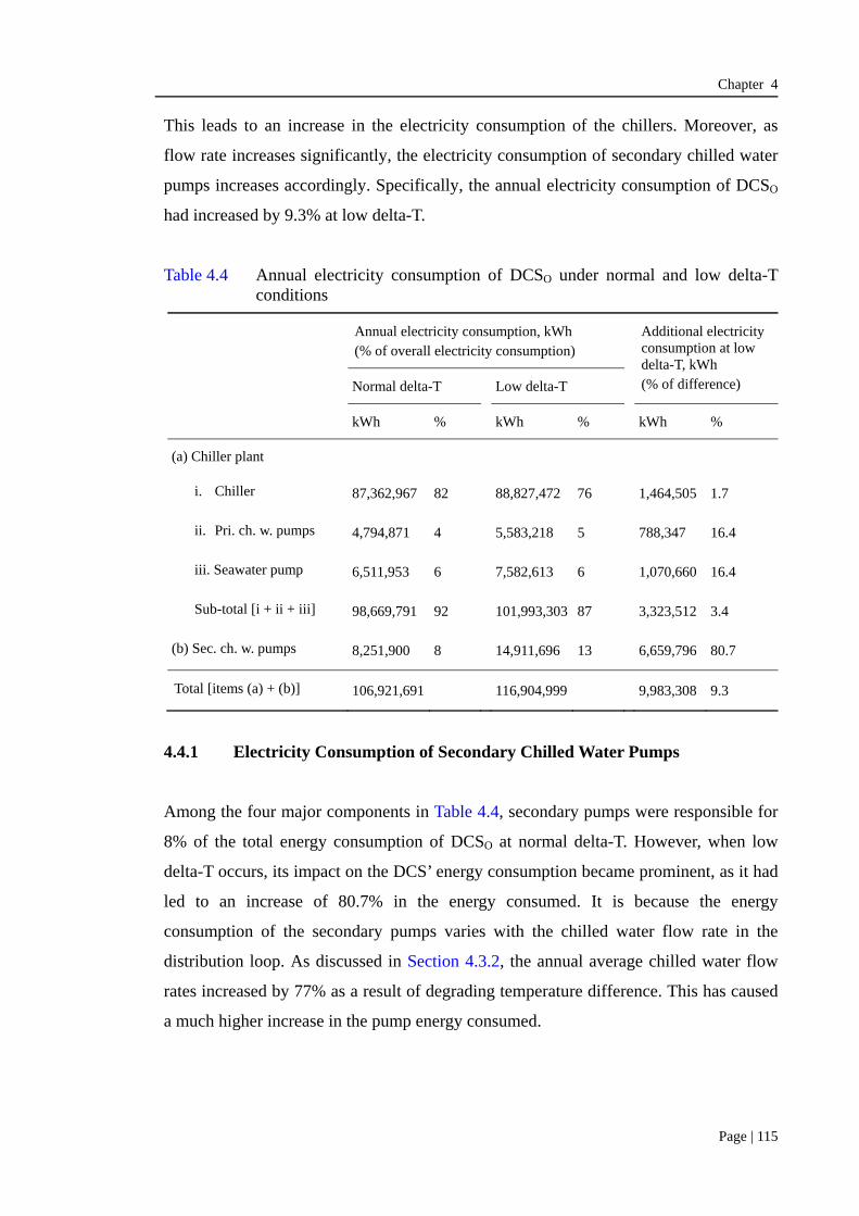
Chapter 4
Page | 115
This leads to an increase in the electricity consumption of the chillers. Moreover, as
flow rate increases significantly, the electricity consumption of secondary chilled water
pumps increases accordingly. Specifically, the annual electricity consumption of DCSO
had increased by 9.3% at low delta-T.
Table 4.4 Annual electricity consumption of DCSO under normal and low delta-T conditions
Annual electricity consumption, kWh (% of overall electricity consumption)
Additional electricity consumption at low delta-T, kWh (% of difference) Normal delta-T Low delta-T
kWh % kWh % kWh %
(a) Chiller plant
i. Chiller 87,362,967 82 88,827,472 76 1,464,505 1.7
ii. Pri. ch. w. pumps 4,794,871 4 5,583,218 5 788,347 16.4
iii. Seawater pump 6,511,953 6 7,582,613 6 1,070,660 16.4
Sub-total [i + ii + iii] 98,669,791 92 101,993,303 87 3,323,512 3.4
(b) Sec. ch. w. pumps 8,251,900 8 14,911,696 13 6,659,796 80.7
Total [items (a) + (b)] 106,921,691 116,904,999 9,983,308 9.3
4.4.1 Electricity Consumption of Secondary Chilled Water Pumps
Among the four major components in Table 4.4, secondary pumps were responsible for
8% of the total energy consumption of DCSO at normal delta-T. However, when low
delta-T occurs, its impact on the DCS’ energy consumption became prominent, as it had
led to an increase of 80.7% in the energy consumed. It is because the energy
consumption of the secondary pumps varies with the chilled water flow rate in the
distribution loop. As discussed in Section 4.3.2, the annual average chilled water flow
rates increased by 77% as a result of degrading temperature difference. This has caused
a much higher increase in the pump energy consumed.

Chapter 4
Page | 116
4.4.2 Electricity Consumption of Chillers
Chillers are the dominant electricity consuming equipment in the DCS. Table 4.4 shows
that for DCSO, low delta-T could lead to an increase of 1.7% in the annual electricity
consumption of chillers. Given the same cooling load, additional chillers are required to
cater for the additional chilled water flow rate at low delta-T. In this regard, the PLR of
chillers is significantly reduced because it is balanced to carry an equal percentage of
the cooling load. As the COP of a constant speed chiller decreases when the PLR
decreases, this has lowered the COP of the chiller.
As discussed in Section 4.3.3, there were 4,670 hours (53% of the total 8,760 hours) in
which one additional chiller was required to be operated and 62 hours (1% of the total
8,760 hours) in which two additional chillers were required at low delta-T in
comparison with those under normal delta-T conditions throughout the year. For the
period in which one additional chiller was required, the average hourly PLR and COP of
the chillers operated under both conditions were simulated based on the chiller model
developed in Chapter 3. The same simulation was performed for the period where two
additional chillers were required.
Table 4.5 Average PLR and COP when one or two additional chillers are operated under normal or low delta-T conditions
One additional chiller Two additional chillers
Normal delta-T Low delta-T Normal delta-T Low delta-T
Average PLR 0.908 0.687 0.993 0.730
Average COP 6.149 5.864 6.173 6.042
It can be seen in Table 4.5 that the average PLR at low delta-T was relatively lower
comparing to that at normal delta-T. Furthermore, the average COP of chillers was also
relatively lower at low delta-T, as compared to the COP in design condition. This
explains why the electricity consumption of chillers operating at low delta-T is
relatively higher in comparison with that of the chillers under normal delta-T condition.

Chapter 4
Page | 117
Nevertheless, the impact of the low delta-T syndrome on the energy consumption of
chillers is moderate in comparison with the secondary pumps. It is because the capacity
of the chillers is sufficiently large enough to cater for the increase in the chilled water
flow rate at low delta-T. In this case, one additional chiller was required to be on for
only 53% of the annual total operating hours.
4.4.3 Electricity Consumption of Primary Chilled Water and Seawater Pumps
In DCSO, constant speed primary chilled water pumps and seawater pumps were
interlocked with dedicated chillers so that they could be switched on and off together.
As discussed in Section 4.3.3, the total operating hours of chillers at low delta-T were
16.4% higher than those of the chillers operating at normal delta-T. This explains why
the annual electricity consumption of the primary chilled water and seawater pumps also
increased proportionally by 16.4%, as shown in Table 4.4.
4.5 Summary
A comparative analysis of the energy performance of P-S and VPF systems was
conducted with reference to the baseline DCSO. The results indicate that the VPF system
was unable to yield any significant saving in the electricity of a large scale DCS such as
DCSO. The main reason is that there were over 80% of the annual pump hours in which
the pumps in both systems were operated at a flow ratio greater than 80%. Under such
circumstances, the variable frequency drive decreases the efficiency of the VSP running
at nearly full speed. It causes the VSP to consume more power than the CSP. This
enables the VSP and CSP in the P-S system to consume less electricity than the VSP in
the VPF system. This has resulted in a slightly lower electricity consumption of the P-S
system, which was 0.5% less than that of the pumps in the VPF system.
Moreover, a comparative analysis of the energy performance of DCSO with a P-S
system under normal or low delta-T conditions was performed. The simulation results
show that chillers represent a major portion of the total electricity consumption of the
DCS. They are then followed by distribution pumps. Primary chilled water pumps and
seawater pumps attribute the least proportion. Compared to a normal delta-T situation,

Chapter 4
Page | 118
the flow rate required to distribute chilled water from the chiller plant was 77% higher
and the annual total electricity consumption of the DCS was increased by 9.3% at low
delta-T.
Under such circumstances, additional chillers have to be staged on to meet the excessive
chilled water flow. More electricity is needed for operating additional chillers to
overcome the cooling capacity deficiency inherent with the degrading temperature issue.
It is because the average hourly PLR and COP of the chillers at low delta-T are
relatively lower than those in design conditions. It is interesting to note that the
percentage of electricity consumption increased by 1.7% as no additional chiller was
required to be operated at low delta-T for about 46% of the total operating hours.
Nevertheless, as chillers were the major energy consuming equipment (76% of the total
electricity consumption) in DCSO, it was worth investigating an optimum chiller system
configuration that could enhance its overall energy efficiency and accommodate the low
delta-T issue.
Secondary pumps were the second largest electricity consuming equipment in DCSO.
Although their proportion of electricity consumption was relatively less as compared to
chillers, their electricity consumption still increased massively by 81% due to the
increase in the chilled water flow rate with degrading temperature difference. Potential
energy saving measures associated with the use of various pumping station
configurations will be studied in the chapters to follow.

Chapter 5
Page | 119
Chapter 5
Effects of Chiller System Configuration on the Energy
Performance of DCSO
5.1 Overview
As it seems inevitable that almost every chiller plant is affected by the low delta-T
syndrome, particularly at low cooling loads, additional chillers and pumps would be
necessary for maintaining a primary flow in the production loop larger than the
secondary flow in the distribution loop. As a result, chillers would operate at a part load
ratio (PLR) smaller than the optimum range where efficiency or COP is maximized.
According to the study in Chapter 4 regarding the energy consumption of the base
DCSO at low delta-T, the chilled water plant was responsible for 87% of the total
electricity consumption of a DCS at low delta-T (Table 4.5). Secondary chilled water
pumps accounted for the remaining 13%. It is therefore imperative to explore ways of
designing a chiller system configuration that can accommodate the low delta-T
syndrome with little loss of efficiency.
As mentioned in Chapter 2, five alternative configurations of chiller system - CA, CB,
CC, CD and CE - were defined (see Table 2.8 in Chapter 2) by varying the influential
design parameters of the chiller system CO in DCSO. These parameters included the
number, cooling capacity and type of chillers. In this chapter, an evaluation of the

Chapter 5
Page | 120
effectiveness of these five configurations in improving the energy performance of DCSO,
with CO taken as the base chiller system configuration is summarized and discussed.
Using the mathematical models developed in Chapter 3, the energy consumption of
these five chiller system configurations was evaluated by simulation for comparison.
The results are shown in Section 5.2. Moreover, a detailed evaluation of the
effectiveness of each design parameter can be found in Sections 5.3, 5.4 and 5.5.
Section 5.6 gives a summary of the comparative analysis.
5.2 Comparison of Annual Total Electricity Consumption of DCSO in
Different Chiller System Configuration Designs
With all other design conditions of DCSO held constant, its chiller system CO was
replaced by five alternative configurations, i.e. CA to CE, in turn, in the study. A
comparison of the annual total electricity consumption of DCSO when incorporated with
each of these five configurations and operating with the low delta-T condition in place,
is given in Table 5.1.
The results show that all the five alternative configurations could lead to positive
savings to different degrees in the annual total electricity consumption of DCSO.
Among these five configurations, use of CB had the smallest reduction in electricity
consumption, i.e. 1.6%. In this case, the number of equally-sized constant speed chillers
was increased from 10 in CO to 15. For CC, its configuration is similar to CB’s except
that the chillers of the former are different in size. This change could help achieve a
2.9% saving in the DCS’ annual electricity consumption, which would be higher when
CB was used. The adoption of variable speed chillers in CA, CD and CE provided a
significant improvement to the DCS’ energy performance. A significant reduction was
achieved by adopting CE, which had led to the highest saving of 11.6%.

Page | 121
Table 5.1 Comparison of the annual total electricity consumption of DCSO using various chiller system configurations at low delta-T
CO CA CB CC CD CE
Design parameter
No. of chiller 10 10 15 15 15 15 Size Equal Equal Equal Unequal Equal Unequal Type Constant
speed Variable
speed Constant
speed Constant
speed Variable
speed Variable
speed
Total chiller hours 33,952 33,952 48,279 37,127 48,279 37,746
Annual electricity consumption, kWh (% of total consumption)
(a) Chiller plant
i. Chiller 88,827,472 (76) 77,216,917 (74) 87,605,334 (76) 86,686,293 (77) 76,705,719 (74) 76,339,990 (75) ii. Pri. ch. w. pump 5,583,218 (5) 5,583,218 (5) 5,289,233 (5) 5,040,671 (4) 5,289,233 (5) 5,107,501 (5) iii. Seawater pump 7,582,613 (6) 7,582,613 (7) 7,198,935 (6) 6,845,941 (6) 7,198,935 (7) 6,936,400 (7)
Total [i + ii + iii] 101,993,303 (87) 90,382,748 (86) 100,093,502 (87) 98,572,905 (87) 89,193,887 (86) 88,383,890 (86)
(b) Sec. ch. w. pump 14,911,696 (13) 14,911,696 (14) 14,911,696 (13) 14,911,696 (13) 14,911,696 (14) 14,911,696 (14)
Total [(a) + (b)] 116,904,999 105,294,444 115,005,198 113,484,601 104,105,583 103,295,586
Difference in electricity consumption w.r.t. CO, kWh (% of total saving)
(a) Chiller plant
i. Chiller - 11,610,555 (-13.1) 1,222,139 (-1.4) 2,141,179 (-2.4) 12,121,753 (-13.6) 12,487,482 (-14.1) ii. Pri. ch. w. pump - - (0.0) 293,985 (-5.3) 542,547 (-9.7) 293,985 (-5.3) 475,717 (-8.5) iii. Seawater pump - - (0.0) 383,678 (-5.1) 736,672 (-9.7) 383,678 (-5.1) 646,214 (-8.5)
Total [i + ii + iii] - 11,610,555 (-11.4) 1,899,802 (-1.9) 3,420,398 (-3.4) 12,799,417 (-12.5) 13,609,413 (-13.3)
(b) Sec. ch. w. pump - - (0.0) - (0.0) - (0.0) - (0.0) - (0.0)
Total difference [(a) + (b)] - 11,610,555 (-9.9) 1,899,802 (-1.6) 3,420,398 (-2.9) 12,799,417 (-10.9 ) 13,609,413 (-11.6)

Chapter 5
Page | 122
Impacts of each chiller system configuration parameter such as the number, cooling
capacity and type of chillers on the energy performance of the DCS were then examined.
Table 5.2 shows a matrix of the cases selected for a more detailed comparison.
Table 5.2 Selection of cases for comparing the energy impact of each design parameter
CO CA CB CC CD CE
Design parameter
No. of chiller 10 10 15 15 15 15
Size Equal Equal Equal Unequal Equal Unequal
Type Constant speed
Variable speed
Constant speed
Constant speed
Variable speed
Variable speed
Comparison based on no. of chiller:
Case O-B
Case A-D
Comparison based on size uniformity:
Case B-C
Case D-E
Comparison based on chiller type:
Case O-A
Case B-D
Case C-E
Remark: “” – configuration selected for evaluating the impact of the respective design parameter
i. Case O-B was formed to compare CO and CB, and case A-D was formed to compare
CA and CD with regard to an increase in the number of chillers.
ii. Case B-C was formed to compare CB and CC, and case D-E was formed to compare
CD and CE with regard to the chiller’s cooling capacity.
iii. Cases O-A, B-D and C-E were formed to compare CO with CA, CB with CD, and CC
with CE respectively with regard to the use of constant and variable speed chillers.
5.3 Effects of Increasing the Number of Chillers – Case O-B and Case A-D
Case O-B and case A-D were selected for a study of the effects of increasing the number
of chillers in the system. The configurations of CO and CB in case O-B, and that of CA
and CD in case A-D were as shown in Table 5.3. A comparison of the annual total

Chapter 5
Page | 123
electricity consumption of DCSO, when configured with the different number of chillers
represented by these cases, is given in Tables 5.4 and 5.5.
Table 5.3 Configuration of chiller systems in cases O-B and A-D
Chiller system Case O-B Case A-D
configuration CO CB CA CD
No. of chiller 10 15 10 15
Size Equal Equal Equal Equal
Cooling capacity 10 x 6,000 RT 15 x 4,000 RT 10 x 6,000 RT 15 x 4,000 RT
(10 x 21,102 kW) (15 x 14,068 kW) (10 x 21,102 kW) (15 x 14,068 kW)
Type Constant speed Constant speed Variable speed Variable speed
Table 5.4 Case O-B: Percentage of electricity saving after addition of chillers in CB
Annual electricity consumption, kWh Annual electricity saving
[CB minus CO]
CO CB kWh %
(a) Chiller plant
i. Chiller 88,827,472 87,605,334 -1,222,139 -1.4
ii. Pri. ch. w. pump 5,583,218 5,289,233 -293,985 -5.3
iii. Seawater pump 7,582,613 7,198,935 -383,678 -5.1
Total [i + ii + iii] 101,993,303 100,093,502 -1,899,802 -1.9
(b) Sec. ch. w. pump 14,911,696 14,911,696 0 0.0
Total [(a) + (b)] 116,904,999 115,005,198 -1,899,802 -1.6
Table 5.5 Case A-D: Percentage of electricity saving after addition of chillers in CD
Annual electricity consumption, kWh
Annual electricity saving[CD minus CA]
CA CD kWh %
(a) Chiller plant
i. Chiller 77,216,917 76,705,719 -511,198 -0.7
ii. Pri. ch. w. pump 5,583,218 5,289,233 -293,985 -5.3
iii. Seawater pump 7,582,613 7,198,935 -383,678 -5.1
Total [i + ii + iii] 90,382,748 89,193,887 -1,188,861 -1.3
(b) Sec. ch. w. pump 14,911,696 14,911,696 0 0.0
Total [(a) + (b)] 105,294,444 104,105,583 -1,188,861 -1.1
In case O-B, a comparison was made of the effects of increasing the number of
equally-sized constant speed chillers from 10 in CO to 15 in CB. It shows a 1.6%

Chapter 5
Page | 124
reduction in the electricity consumption of DCSO after adopting CB instead of CO. For
case A-D, more equally-sized variable speed chillers were used in CD and this led to a
saving of 1.1% in electricity consumption as compared to using CA.
This indicates that the use of a greater number of equally-sized chillers with a smaller
cooling capacity (i.e. 15 x 4,000 RT (14,068 kW)), as in CB and CD, can contribute to a
reduction in the electricity consumption of DCSO at low delta-T.
5.3.1 Electricity Consumption of Chillers
CO and CB comprised 10 x 6,000 RT (21,102 kW) and 15 x 4,000 RT (14,068 kW)
equally-sized constant speed chillers, respectively. While a chiller plant is running, one
additional chiller will be staged on when the cooling load exceeds the total cooling
capacity of the operating chillers. The number of available steps of total cooling output
capacity equals the total number of equally-sized chillers installed. Hence, the number
of steps of CB is higher, i.e. 15. There is then a greater freedom to adjust the number of
chillers in CB to achieve a higher COP while meeting the variable cooling demand. As
Figure 5.1 shows, the average COP values of the constant speed chillers in CB at
different PLR were slightly higher than those of CO. This explains why the annual
electricity consumption of the chillers in CB was 1.4% less than that of CO.
Figure 5.1 Average COP of constant speed chillers in CO and CB at different PLR

Chapter 5
Page | 125
For case A-D where variable speed chillers were used, the saving in electricity
consumption of the chillers after increasing their number from 10, as in CA to 15, as in
CD, was only 0.7%. This percentage is relatively small when compared to case O-B
(1.4%) where constant speed chillers were adopted. This is because of the higher
part-load COP of variable speed chillers compared to constant speed chillers, as shown
in Figure 5.2. As shown in Table 2.5 in Chapter 2, the cooling load on the DCS was
below 50% for 77% of the total 8,760 operating hours in a year. Since the chillers were
operated at part load for most of the time, the use of variable speed chillers could help
significantly reduce the electricity consumption of the DCS, as in case CA or CD. Figure
5.3 shows that the average COP of the chillers in CA and CD were higher at low load in
comparison with those in CO and CB (Figure 5.1). This had led to a smaller difference in
the electricity consumption between CA and CD.
Moreover, this illustrates that the effect of using a greater number of chillers could be
insignificant in reducing electricity consumption if the plant is already using variable
speed chillers.
Figure 5.2 COP of constant and variable speed chillers with a cooling capacity of
4,000 RT (14,068 kW)

Chapter 5
Page | 126
Figure 5.3 Average COP of variable speed chillers in CA and CD at different PLR
5.3.2 Electricity Consumption of Primary Chilled Water Pumps and Seawater
Pumps
As primary chilled water pumps and seawater pumps are interlocked with their
dedicated chillers during operation, their total pump hours are the same as the chiller’s
total chiller hours. With reference to Tables 5.6 and 5.7, for cases O-B and A-D, the total
pump hours of these pumps in cases CB and CD were longer, i.e. both were 42% more
than those in CO and CA. However, in both cases, their electricity consumption was
5.3% and 5.1% less than that in CO and CA. The reason is that the power demand of the
pumps in CB and CD was about 33% less than that in CO and CA. In other words,
although the pumps in CB and CD had relatively longer pump hours, they consumed less
electricity in comparison with those in CO and CA.
Having said that, however, it should be re-emphasized that primary chilled water pumps
and seawater pumps constitute a much smaller portion of the annual total electricity
consumption of the plant when compared to chillers. The electricity saving of these two
types of pumps, therefore, would not significantly affect the annual total electricity
consumption of the DCS.

Chapter 5
Page | 127
Table 5.6 Operating chiller hours of chillers and electricity saving of the primary chilled water and seawater pumps in case O-B
CO CB Difference % difference
(CB minus CO)
Total chiller hour 33,952 48,279 +14,327 +42
Primary chilled water pump
Unit power demand, kW 164.6 109.6 -55 -33.4
Annual electricity consumption, kWh
5,583,218 5,289,223 -293,985 -5.3
Seawater pump
Unit power demand, kW 223.3 149.1 -74.2 -33.2
Annual electricity consumption, kWh
7,582,613 7,198,935 -383,678 -5.1
Table 5.7 Operating chiller hours and electricity saving of the primary chilled water and seawater pumps in case A-D
CA CD Difference % difference
(CD minus CA)
Total chiller hour 33,952 48,279 +14,327 +42
Primary chilled water pump
Unit power demand, kW 164.6 109.6 -55 -33.4
Annual electricity consumption, kWh
5,583,218 5,289,223 -293,985 -5.3
Seawater pump
Unit power demand, kW 223.3 149.1 -74.2 -33.2
Annual electricity consumption, kWh
7,582,613 7,198,935 -383,678 -5.1
5.4 Effects of Uniformity in Chiller Size – Case B-C and Case D-E
Cases B-C and D-E were selected for examining the effect of unequally-sized chillers
on the total energy consumed. The configuration details of CB and CC in case B-C, and
those of CD and CE in case D-E are given in Table 5.8.

Chapter 5
Page | 128
Table 5.8 Configuration of chiller systems in cases B-C and D-E
Chiller system configuration
Case B-C Case D-E
CB CC CD CE
No. of chiller 15 15 15 15
Size Equal Unequal Equal Unequal
Cooling capacity 15 x 4,000 RT (15 x 14,068 kW)
5 x 2,000 RT (5 x 7,034 kW)
5 x 4,000 RT (5 x 14,068 kW)
5 x 6,000 RT (5 x 21,102 kW)
15 x 4,000 RT (15 x 14,068 kW)
5 x 2,000 RT (5 x 7,034 kW)
5 x 4,000 RT (5 x 14,068 kW)
5 x 6,000 RT (5 x 21,102 kW)
Type Constant speed Constant speed Variable speed Variable speed
Case B-C represents a comparison of CB and CC, both of which consisted of 15 constant
speed chillers. The only difference is that the chillers in CB were of equal size, i.e. 15 x
4,000 RT (14,068 kW) and the chillers in CC had three different cooling capacities, i.e. 5
x 2,000 RT (7,034 kW), 5 x 4,000 RT (14,068 kW) and 5 x 6,000 RT (21,102 kW).
The configurations of CB and CD were the same, except that the chillers in CD were of
variable speed. Similarly, CC and CE had the same configuration, as the only difference
was in the chiller type (constant speed versus variable speed).
In case B-C, a comparison was made regarding the use of unequally-sized constant
speed chillers in CC. It was found that the adoption of CC, instead of CO, had resulted in
a 1.3% reduction in the electricity consumption of DCSO. For case D-E, unequally-sized
variable speed chillers were used in CE, which could lead to a saving of 0.8% in
electricity as compared to using CD.
As shown in Tables 5.9 and 5.10, the annual total electricity consumptions of DCSO
designed with CC and CE and operating with low delta-T were 1.3% and 0.8% lower
than those in CB and CD respectively.

Chapter 5
Page | 129
Table 5.9 Case B-C: Percentage of annual electricity saving after using unequally-sized chillers in CC
Annual electricity consumption, kWh
Annual electricity saving [CC minus CB]
CB CC kWh %
(a) Chiller plant
i. Chiller 87,605,334 86,686,293 -919,040 -1.0
ii. Pri. ch. w. pump 5,289,233 5,040,671 -248,562 -4.7
iii. Seawater pump 7,198,935 6,845,941 -352,994 -4.9
Total [i + ii + iii] 100,093,502 98,572,905 -1,520,596 -1.5
(b) Sec. ch. w. pump 14,911,696 14,911,696 0 0.0
Total [(a) + (b)] 115,005,198 113,484,601 -1,520,596 -1.3
Table 5.10 Case D-E: Percentage of annual electricity saving after using
unequally-sized chillers in CE
Annual electricity consumption, kWh
Annual electricity saving [CE minus CD]
CD CE kWh %
(a) Chiller plant
i. Chiller 76,705,719 76,339,990 -365,729 -0.5
ii. Pri. ch. w. pump 5,289,233 5,107,501 -181,732 -3.4
iii. Seawater pump 7,198,935 6,936,400 -262,536 -3.6
Total [i + ii + iii] 89,193,887 88,383,890 -809,996 -0.9
(b) Sec. ch. w. pump 14,911,696 14,911,696 0 0.0
Total [(a) + (b)] 104,105,583 103,295,586 -809,996 -0.8
5.4.1 Electricity Consumption of Chillers
CC and CE comprised unequally-sized chillers of three cooling capacities. A total of 215
steps or chiller combinations were involved in the simulation process to achieve
different total cooling capacities. This increased the opportunity to optimize the
operation of chillers by keeping their operation in the near full load and high COP
region while meeting various cooling load requirements.
Table 5.11 lists out the distribution of average PLR of the chillers operating around the
8760 hours of a year in cases B-C and D-E. In case B-C, the 15 identical chillers in CB
operated at a near full load range, i.e. the PLR ranged from 0.8 to 1, for 22% (=20% +
2%) of the 8,760 operating hours in a year. This figure rose to 29% (=25% + 4%) in CC
with the use of 15 unequally-sized chillers. A similar increase can be found in case D-E

Chapter 5
Page | 130
where the percentage increased from 22% (=20% + 2%) in CD to 28% (=25% + 3%) in
CE.
Table 5.11 Distribution of average PLR of the chillers operating around the 8760
hours of a year in cases B-C and D-E
Case B-C Case D-E
Part load ratio CB CC CD CE
≤0.1 0% 0% 0% 0%
0.1 < PLR ≤ 0.2 0% 0% 0% 0%
0.2 < PLR ≤ 0.3 11% 8% 11% 8%
0.3 < PLR ≤ 0.4 3% 2% 3% 2%
0.4 < PLR ≤ 0.5 6% 3% 6% 3%
0.5 < PLR ≤ 0.6 7% 6% 7% 6%
0.6 < PLR ≤ 0.7 18% 16% 18% 21%
0.7 < PLR ≤ 0.8 32% 36% 32% 32%
0.8 < PLR ≤ 0.9 20% 25% 20% 25%
0.9 < PLR ≤ 1.0 2% 4% 2% 3%
As shown in Figure 5.4, the average COP of the constant speed chillers in CC at
different PLR was slightly higher than that in CB. This corresponds to the 1% reduction
in the electricity consumption of chillers in CC as compared to CB (see Table 5.9).
Figure 5.4 Average COP of constant speed chillers in CB and CC at different PLR

Chapter 5
Page | 131
For case D-E, Figure 5.5 shows that the average COP of the variable speed chillers in
CE at different PLR was higher than that in CD. Unequally-sized chillers in CE could
reduce the electricity consumption of chillers by 0.5% in comparison with CD.
Figure 5.5 Average COP of variable speed chillers in CD and CE at different PLR
5.4.2 Electricity Consumption of Primary Chilled Water Pumps and Seawater
Pumps
As shown in Tables 5.12 and 5.13, the reduction in the annual electricity consumption of
the primary chilled water pumps and seawater pumps in CC and CE ranged from 3.4% to
4.9% when compared to CB and CD. The reasons were as follows.
i. Three sizes of primary chilled water pumps were selected for serving the
chillers in CC and CE, which were with three different cooling capacities. There
were five pumps of each size and the unit power demand values of the three
pump sizes were 56.9 kW, 109.6 kW and 164.4 kW respectively. The weighted
averages of the unit power demand in CC and CE were 110.3 kW (i.e. (5 x 56.9
kW + 5 x 109.6 kW + 5 x 164.4 kW)/15) as shown in Tables 5.12 and 5.13,
which were slightly higher (i.e. 0.6%) than the unit power demand of 109.6 kW
of the pumps in CB and CD. The difference was due to the small pumps selected

Chapter 5
Page | 132
for lower chilled water flow rate as they are generally less efficient than the
large pumps given that their pressure head is the same.
Each chiller was also equipped with a seawater pump of a matching size. There
were five pumps of each size in CC and CE and the unit power demand values
of the three pump sizes were 75.3 kW, 149.1 kW and 223.3 kW respectively.
The weighted average of the unit power demand was 149.2 kW (i.e. (5 x 75.3
kW + 5 x 149.1 kW + 5 x 223.3 kW)/15) as shown in Tables 5.12 and 5.13,
which was also slightly higher than the unit power demand of these pumps in
CB and CD, i.e. 149.1 kW.
ii. On the other hand, the chillers in CC and CE designed with unequal cooling
capacities could allow more combinations of different total cooling capacities to
meet the chilled water flow requirement. This is particularly useful when the low
delta-T syndrome occurs as the chilled water flow rate becomes higher than the
design value. The number of chillers required to meet the flow rate can also be
reduced. The total chiller hours in CC and CE were 22% to 23% fewer in
comparison with those in CB and CD respectively.
For example, to meet a required flow rate at 2.47m3/s, six sets of 4,000 RT
(14,068 kW) chillers were required in CB to be operated and the total design
flow rate was 2.87m3/s (6 x 0.4784m3/s), which was 16% higher than the
required flow rate. However, for CC, only four unequally-sized chillers (i.e. 1 x
4,000 RT (14,068 kW) and 3 x 6,000 RT (21,102 kW)) were required. The total
design flow rate in CC was 2.63m3/s, which was slightly higher, i.e. 6.5%, than
the required flow rate.
iii. As the total pump hours of the primary pumps correspond to the total chiller
hours of the chillers, which they are dedicated to serve, the total pump hours of
the pumps in CC and CE were far fewer than those in CB and CD, with a
difference of 22-23% (see Tables 5.12 and 5.13). This could help to reduce their
electricity consumption and offset the slight increase in power demand from the
primary chilled water and seawater pumps.

Chapter 5
Page | 133
Table 5.12 Chiller hours and electricity saving of the primary chilled water and seawater pumps in case B-C
CB CC Difference (CC minus CB)
% Difference
Total chiller hour 48,279 37,127 -11,152 -23%
Primary chilled water pump
Weighted average of unit power demand, kW
109.6 110.3 +0.7 +0.6%
Annual electricity consumption, kWh 5,289,233 5,040,671 -248,562 -4.7%
Seawater pump
Weighted average of unit power demand, kW
149.1 149.2 ~0
Annual electricity consumption, kWh 7,198,935 6,845,941 -352,994 -4.9%
Table 5.13 Chiller hours and electricity saving of the primary chilled water and seawater pumps in case D-E
CD CE Difference (CE minus CD)
% Difference
Total chiller hour 48,279 37,746 -10,533 -22%
Primary chilled water pump
Weighted unit power demand, kW 109.6 110.3 +0.7 +0.6%
Annual electricity consumption, kWh 5,289,233 5,107,501 -181,732 -3.4%
Seawater pump
Weighted unit power demand, kW 149.1 149.2 ~0
Annual electricity consumption, kWh 7,198,935 6,936,400 -262,536 -3.6%
5.5 Effects of Variable Speed Chillers
Cases O-A, B-D and C-E were set up for studying the effects of variable speed chillers.
The configuration details of CO and CA in case O-A, CB and CD in case B-D, and CC and
CE in case C-E were as shown in Table 5.14.

Chapter 5
Page | 134
Table 5.14 Configuration of the chiller systems in cases O-A, B-D, and C-E
Chiller system configuration
Case O-A Case B-D Case C-E
CO CA CB CD CC CE
No. of chiller 10 10 15 15 15 15
Size Equal Equal Equal Equal Unequal Unequal
Cooling capacity
10 x 6,000 RT (10 x 21,102 kW)
10 x 6,000 RT (10 x 21,102 kW)
15 x 4,000 RT (15 x 14,068 kW)
15 x 4,000 RT (15 x 14,068 kW)
5 x 2,000 RT (5 x 7,034 kW)
5 x 4,000 RT (5 x 14,068 kW)
5 x 6,000 RT (5 x 21,102 kW)
5 x 2,000 RT (5 x 7,034 kW)
5 x 4,000 RT (5 x 14,068 kW)
5 x 6,000 RT (5 x 21,102 kW)
Type Constant speed
Variable speed
Constant speed
Variable speed
Constant speed
Variable speed
In case O-A, CO and CA comprised 10 x 6,000 RT (21,102 kW) chillers. These chillers
were constant speed in CO and variable speed in CA. The characteristics of case B-D
were similar except for the number of chiller; 15 x 4,000 RT (14,068 kW) chillers were
adopted for CB and CD. For case C-E, configurations CC and CE comprised 15
unequally-sized chillers, i.e. 5 x 2,000 RT (7,034 kW), 5 x 4,000 RT (14,068 kW) and 5
x 6,000 RT (21,102 kW) chillers. These chillers were constant speed in CC and variable
speed in CE.
It can be seen from Tables 5.15, 5.16 and 5.17 that application of variable speed chillers
led to a significant reduction in the annual total electricity consumption of DCSO,
between 9% and 9.9% in comparison with the use of constant speed chillers across all
the three cases.

Chapter 5
Page | 135
Table 5.15 Electricity saving resulting from using variable speed chillers in case O-A
Annual electricity consumption, kWh
Annual electricity saving [CA minus CO]
CO CA kWh %
(a) Chiller plant
i. Chiller 88,827,472 77,216,917 -11,610,555 -13.1
ii. Pri. ch. w. pump 5,583,218 5,583,218 0 0
iii. Seawater pump 7,582,613 7,582,613 0 0
Total [i + ii + iii] 101,993,303 90,382,748 -11,610,555 -11.4
(b) Sec. ch. w. pump 14,911,696 14,911,696 0 0
Total [(a) + (b)] 116,904,999 105,294,444 -11,610,555 -9.9
Table 5.16 Electricity saving resulting from using variable speed chillers in case B-D
Annual electricity consumption, kWh
Annual electricity saving [CD minus CB]
CB CD kWh %
(a) Chiller plant
i. Chiller 87,605,334 76,705,719 -10,899,615 -12.4
ii. Pri. ch. w. pump 5,289,233 5,289,233 0 0
iii. Seawater pump 7,198,935 7,198,935 0 0
Total [i + ii + iii] 100,093,502 89,193,887 -10,899,615 -10.9
(b) Sec. ch. w. pump 14,911,696 14,911,696 0 0
Total [(a) + (b)] 115,005,198 104,105,583 -10,899,615 -9.5
Table 5.17 Electricity saving resulting from using variable speed chillers in case C-E
Annual electricity consumption, kWh
Annual electricity saving [CE minus CC]
CC CE kWh %
(a) Chiller plant
i. Chiller 86,686,293 76,339,990 -10,346,303 -11.9
ii. Pri. ch. w. pump 5,040,671 5,107,501 +66,830 +1.3
iii. Seawater pump 6,845,941 6,936,400 +90,458 +1.3
Total [i + ii + iii] 98,572,905 88,383,890 -10,189,015 -10.3
(b) Sec. ch. w. pump 14,911,696 14,911,696 0 0
Total [(a) + (b)] 113,484,601 103,295,586 -10,189,015 -9

Chapter 5
Page | 136
The application of variable speed chillers in CA, CD and CE could lead to a significant
reduction in the annual total electricity consumption of DCSO by 9.9%, 9.5% and 9%
compared respectively with CO, CB and CC, which comprised constant speed chillers.
Variable speed chillers have better energy performance due to the following reasons.
i. In a constant speed chiller, inlet guide vanes are traditionally used to throttle
refrigerant at the inlet of the compressor to vary the compressor capacity at part
load. As the vanes move from open to close, they become a restriction and reduce
the compressor’s capacity and efficiency.
For a variable speed chiller, a variable speed drive is adopted to vary the speed of
the impeller of the compressor to meet various loads at part load. The power
demand of the compressor can be significantly reduced when the speed of the
impeller reduces at part load. The impeller must produce an adequate pressure
differential (lift) to move the refrigerant from the low-pressure side (evaporator)
to the high-pressure side (condenser). It is this lift that determines the minimum
speed of the impeller. The lower the lift, i.e. the closer the temperature difference
between the evaporator and the condenser, the slower the impeller can rotate.
When the impeller is at the slowest possible speed, further reductions in capacity
are obtained by using the inlet guide vanes.
ii. Figure 5.6 illustrates the part load performance curves of a constant and a variable
speed chiller, each of which was rated for 2,000 RT (7,034 kW) output at the
design chilled water supply temperature of 5oC. The curve in Figure 5.6 shows the
performance of these chillers when they operated at the condenser water entering
temperature of 20oC, 25oC or 30oC.

Chapter 5
Page | 137
Figure 5.6 Part load performance of constant and variable speed chillers with different condenser water entering temperatures
It can be seen that the COP of the variable speed chiller is higher than that of the
constant speed chiller, particularly when the condenser water entering temperature
is at 20oC. The optimum COP of variable speed chillers occurs when the PLR is
around 0.6. This characteristic can be utilized to enhance the energy performance
of the chiller system operating at part load, to alleviate the low delta-T syndrome,
particularly at low cooling loads.
Table 5.18 shows the difference in COP between the constant and variable speed
chillers while operating under different condenser water entering temperatures.
The COP difference at part load diminished as the condenser water entering
temperature increased from 20 oC to 30oC.

Chapter 5
Page | 138
Table 5.18 Difference in COP between constant and variable speed chillers with different condenser water entering temperatures
Condenser water entering temp Part load ratio
20% 40% 60% 80% 100%
20oC 29% 28% 19% 9% 0%
25oC 9% 12% 9% 5% 0%
30oC 2% 4% 4% 2% 0%
Figure 5.6 shows also that the increase in the COP of the variable speed chiller, as
the condenser water entering temperature was reduced from 30oC to 20oC, was far
more significant than that of the constant speed chiller. Since direct seawater
cooling was used in DCSO for heat rejection, the condenser water entering
temperature was in fact the seawater temperature. As mentioned in Table 2.6 of
Chapter 2, the seawater temperature of Hong Kong would stay below 25oC for
over 50% of the total 8,760 operating hours in a year. Therefore, these conditions
are conducive to achieving great energy saving by using variable speed chillers.
iii. Figure 5.7 shows that the average COP of the variable speed chillers in CA at
different PLR was higher than that of the constant speed chillers in CO,
particularly at low load. This explains why CA could help reduce the annual total
electricity consumption of DCSO by 10% in comparison with CO. The same
explanation applies to cases B-D and C-E.
Figure 5.7 Average COP of the constant and variable speed chillers in CO and CA

Chapter 5
Page | 139
For case C-E, both CC and CE were designed with chillers of unequal cooling capacities.
The total chiller hours of the variable speed chillers in CE were greater than those of the
constant speed chillers in CC (see Table 5.19). Energy simulation results indicate that it
would be more energy efficient to operate more variable speed chillers as in CE. This
result may appear counterintuitive, as conventional wisdom is to run as few chillers as
possible. This conception, however, is true for constant speed chillers only, because
variable speed chillers can be more efficient at low load, particularly when the
condenser entering water temperature is low (Taylor, 2012). In this regard, although the
electricity consumption of primary chilled water and seawater pumps was slightly
higher in CE than that in CC, this was offset by the substantial gain in electricity saving
through the use of variable speed chillers in the former case.
Table 5.19 Operating hours of chillers in case C-E
CC CE Difference (%) [CE minus CC]
Total chiller hour 37,127 37,746 +619 (+1.7%)
5.6 Summary
Optimization of chiller system configuration was one of the three energy efficiency
enhancement measures evaluated in this study to improve the energy performance of
DCSO and accommodate the inevitable low delta-T issue. Initially, five different chiller
system configurations were established by means of changing the design parameters
such as the number, cooling capacity and type of chillers (constant or variable speed).
Simulation was performed to evaluate the effectiveness of each type of configuration in
enhancing the energy performance of DCSO with reference to a base chiller system
design CO.
In a comparative analysis of the annual total electricity consumption of DCSO when it
was incorporated with one of the five proposed chiller system configurations, i.e. CA to
CE, with low delta-T issue in place, it was found that chiller system configuration CE,
consisting of 15 unequally-sized variable speed chillers, i.e. 5 x 2,000 RT (7,034 kW), 5
x 4,000 RT (14,068 kW) and 5 x 6,000 RT (21,102 kW), performed the best in terms of

Chapter 5
Page | 140
energy saving. It could reduce 11.7% of the annual total electricity consumption of
DCSO even when low delta-T occurred.
For cases O-B, A-D, B-C and D-E, the use of a larger number of or unequally-sized
chillers would increase the flexibility of operating the chillers to cope with the variable
cooling load requirements. The greater the number of chillers (or the number of chillers
with different cooling capacities), the higher the average PLR and hence the COP of the
operating chillers. However, the adoption of more or unequally-sized chillers could only
lead to a limited saving in the annual total electricity consumption of DCSO, as this
saving was less than 2%, when compared to using the basic design CO at low delta-T.
There is also a limit in operation so that switching the chillers on and off cannot be done
at a frequent pace.
On the other hand, for cases O-A, B-D and C-E, results indicate that the variable speed
chillers could dramatically improve the part load performance of the chillers and save a
substantial amount of electricity for DCSO, i.e. between 9% and 9.9%. As a result,
although the low delta-T issue is inevitable, particularly at low cooling loads, the high
energy efficiency of the variable speed chillers at part load can help lessen the impacts
caused by degrading delta-T.
The use of more variable speed chillers with different cooling capacities can lead to a
higher initial capital and operating cost in comparison with the base design in CO.
Therefore, a financial analysis was performed to find out whether the total electricity
cost saving could offset the higher initial costs. This issue is further explored in Chapter
8.

Chapter 6
Page | 141
Chapter 6
Effects of Pumping Station Configuration on the Energy
Performance of DCSO
6.1 Overview
As discussed in Chapter 4, the annual average value of the hourly chilled water flow
rate demand of the hypothetical district, when the DCS was suffering from the low
delta-T problem, increased by 77% as compared to the normal delta-T condition.
Consequently, the electricity consumption of the secondary chilled water pumps was
significantly increased by 81%. Energy saving measures, in particular those related to
pumping station configuration, are of critical importance in a study of DCS energy use.
In this chapter, the effects of different pumping station configurations on the energy
performance of DCSO are investigated. Moreover, a configuration that can mitigate the
impacts of the low delta-T on the energy performance of DCSO is discussed.
From Chapter 3, the base pumping station system in DCSO consisted of one main
pumping station, denoted as PS1-0, was located immediately downstream of the chiller
plant. This pumping station was equipped with 10 equally-sized variable speed chilled
water pumps. Two design schemes were examined in this chapter to evaluate their
effectiveness in mitigating the impacts of low delta-T on the energy performance of

Chapter 6
Page | 142
DCSO. The first scheme was to adopt multiple pumping stations instead of a single
pumping station, and the location of stations could be anywhere at the chilled water
supply and return sides of the distribution loop. To further optimize the design of DCSO,
the second scheme was to adopt an unequal number of pumps in each pumping station.
Regarding the design of multiple pumping stations, the 1,024 combinations of pumping
station could generate a total of 431,940 pumping station arrangements, based on the
variation in the number of pumps, i.e. in groups of 5, 10 or 15, in each pumping station.
As it would require a prohibitively large amount of time and effort in simulating the
energy performance of each of the 431,940 pumping station arrangements, a hydraulic
gradient approach was used to identify the combinations that were technically feasible
for simulation. A detailed account of this approach is given in Section 6.2. Another
design scheme, that is to vary the number of pumps in each pumping station, is
presented in Section 6.3. Mathematically, calculation for an optimum pumping station
design is a very complicated issue, as it involves over hundred thousands of pumping
station arrangements for analysis. As a result, based on the mathematical models
developed in Chapter 3, an optimization program using Excel VBA was developed to
calculate the annual electricity consumption of different pumping station combinations,
as in Section 6.4. Their energy performance is discussed in Section 6.5.
6.2 Multiple Pumping Station Design
As shown in Figure 2.7 of Chapter 2, except that of the main pumping station, there
were 11 possible locations at the chilled water supply and return sides for placing the
booster pumping station to distribute chilled water to all buildings and return it to the
central plant. Based on the calculation in Table 2.10, a total of 1,024 “combinations” of
pumping station location could be derived for the use of one to six pumping stations. In
this chapter, the phrase “pumping station combination” refers specifically to the
grouping of pumping stations according to their location in the distribution loop.
In view of the massive number of combinations to be involved in simulating the energy
performance of each combination with different design parameters, a hydraulic gradient
approach was adopted to identify only those technically feasible combinations.

Chapter 6
Page | 143
6.2.1 Hydraulic Gradient Characteristics of Chilled Water Distribution
Network
As discussed in Section 3.4.2, the flow rate and pressure head of the secondary
distribution pumps are consistently regulated by varying pump speed to match the
changes in the chilled water demand. A differential pressure transmitter has to be
installed in the critical branch, typically the furthest branch, so that any change in the
flow rate demand, which is reflected by a change in the differential pressure across the
critical branch, can be detected and used as a reference signal for controlling the
secondary pump speed. As no previous research studies could be identified regarding
the appropriate location for the differential pressure transmitters in a DCS, the
transmitters in this study were located in all the intermediate branches in the chilled
water distribution network model developed in Chapter 3. The aim was to simulate the
pressure difference across each branch so as to find out a critical branch. Results show
that the critical branch was still located at the furthest end of the chilled water
distribution network. The differential pressure across the critical branch was maintained
at a constant level. Furthermore, pressure drop across all the intermediate branches
should also be the same as the pressure drop across the critical branch.
In this regard, a screening strategy of using a hydraulic gradient approach (Rishel et at,
2006) was applied to calculate the pressure head and flow rate of each pumping station,
and the differential pressure across the heat exchangers. Those combinations of location
that could not meet the minimum pressure were removed from the analysis.
6.2.2 Identified Combinations of Pumping Station
Based on the chilled water distribution network model developed in Chapter 3, the
pressure difference across all the heat exchangers was simulated and checked against
the minimum differential pressure, i.e. DPmin. Taking the case of three pumping stations
in the secondary chilled water network as an example, one of the pumping stations was
a main station and there were 55 possible combinations, as shown in Table 2.10, for
locating the other two pumping stations in the network. Figure 6.1 represents one of the
55 combinations that could meet the minimum differential pressure requirement. The

Chapter 6
Page | 144
same simulation was performed for the other 54 combinations. It was found that only
38% (i.e. 21 of the 55) of the combinations could meet the requirement. The simulation
results of the network designed with one, two, four, five or six pumping stations are
shown in Table 6.1. Only 14% (i.e. 140 of the total 1,024) combinations were found to
be technically feasible in maintaining the minimum differential pressure across the heat
exchangers. A detailed illustration of the exact pumping station location using these 140
combinations is given in Table 6.2.
Figure 6.1 Examples of a pressure gradient diagram showing: (a) the location of one main pumping station and two booster pumping stations; and (b) their pressure gradient in the distribution loop

Chapter 6
Page | 145
Table 6.1 Number of pumping station combinations that are technically feasible in meeting the minimum pressure differential requirement
No. of pumping station
No. of possible combination based on location
No. of combination that can meet the minimum pressure differential requirement
(% of success)
1 1 1 (100%)
2 11 7 (64%)
3 55 21 (38%)
4 165 37 (22%)
5 210 44 (13%)
6 462 30 (6%)
Total 1,024 140 (14%)
Table 6.1 shows that the rate of success in meeting the differential pressure requirement
decreases when the number of pumping station increases. Failure cases often occurred
when the pumping station was located at the far end of the centralized chiller plant. It is
because the system’s pressure head decreases as the distance from the central DCS plant
increases. Meanwhile, the pumping station has to maintain a minimum pressure drop
across the heat exchangers in each building. Therefore, there will be a situation in which
system pressure decreases to a value in a location where the differential pressure
between the chilled water supply and return cannot achieve the minimum value with a
booster pumping station.
The hydraulic pressure diagrams in Figures 6.2, 6.3, 6.4 and 6.5 provide some examples
of the successful and failure cases in the following four different situations, which have
included all the possible location combinations.

Chapter 6
Page | 146
Table 6.2 Combination of pumping station (PS) location that is technically feasible
Location of pumping station No. of PS
Designation of PS combination
Chilled water supply side Chilled water return side
PS1,s PS2,s PS3,s PS4,s PS5,s PS6,s PS1,r PS2,r PS3,r PS4,r PS5,r PS6,r
1 PS 1-1 ● 2 PS 2-1 ● ●
PS 2-2 ● ● PS 2-3 ● ● PS 2-4 ● ● PS 2-5 ● ● PS 2-6 ● ● PS 2-7 ● ●
3 PS 3-1 ● ● ● PS 3-2 ● ● ● PS 3-3 ● ● ● PS 3-4 ● ● ● PS 3-5 ● ● ● PS 3-6 ● ● ● PS 3-7 ● ● ● PS 3-8 ● ● ● PS 3-9 ● ● ● PS 3-10 ● ● ● PS 3-11 ● ● ● PS 3-12 ● ● ● PS 3-13 ● ● ● PS 3-14 ● ● ● PS 3-15 ● ● ● PS 3-16 ● ● ● PS 3-17 ● ● ● PS 3-18 ● ● ● PS 3-19 ● ● ● PS 3-20 ● ● ● PS 3-21 ● ● ●
4 PS 4-1 ● ● ● ● PS 4-2 ● ● ● ● PS 4-3 ● ● ● ● PS 4-4 ● ● ● ● PS 4-5 ● ● ● ● PS 4-6 ● ● ● ● PS 4-7 ● ● ● ● PS 4-8 ● ● ● ● PS 4-9 ● ● ● ● PS 4-10 ● ● ● ● PS 4-11 ● ● ● ● PS 4-12 ● ● ● ● PS 4-13 ● ● ● ● PS 4-14 ● ● ● ● PS 4-15 ● ● ● ● PS 4-16 ● ● ● ● PS 4-17 ● ● ● ● PS 4-18 ● ● ● ● PS 4-19 ● ● ● ● PS 4-20 ● ● ● ●

Chapter 6
Page | 147
Table 6.2 Combination of pumping station (PS) location that is technically feasible (Con’t)
Location of pumping station No. of PS
Designation of PS combination
Chilled water supply side Chilled water return side
PS1,s PS2,s PS3,s PS4,s PS5,s PS6,s PS1,r PS2,r PS3,r PS4,r PS5,r PS6,r
4 PS 4-21 ● ● ● ● PS 4-22 ● ● ● ● PS 4-23 ● ● ● ● PS 4-24 ● ● ● ● PS 4-25 ● ● ● ● PS 4-26 ● ● ● ● PS 4-27 ● ● ● ● PS 4-28 ● ● ● ● PS 4-29 ● ● ● ● PS 4-30 ● ● ● ● PS 4-31 ● ● ● ● PS 4-32 ● ● ● ● PS 4-33 ● ● ● ● PS 4-34 ● ● ● ● PS 4-35 ● ● ● ● PS 4-36 ● ● ● ● PS 4-37 ● ● ● ●
5 PS 5-1 ● ● ● ● ● PS 5-2 ● ● ● ● ● PS 5-3 ● ● ● ● ● PS 5-4 ● ● ● ● ● PS 5-5 ● ● ● ● ● PS 5-6 ● ● ● ● ● PS 5-7 ● ● ● ● ● PS 5-8 ● ● ● ● ● PS 5-9 ● ● ● ● ● PS 5-10 ● ● ● ● ● PS 5-11 ● ● ● ● ● PS 5-12 ● ● ● ● ● PS 5-13 ● ● ● ● ● PS 5-14 ● ● ● ● ● PS 5-15 ● ● ● ● ● PS 5-16 ● ● ● ● ● PS 5-17 ● ● ● ● ● PS 5-18 ● ● ● ● ● PS 5-19 ● ● ● ● ● PS 5-20 ● ● ● ● ● PS 5-21 ● ● ● ● ● PS 5-22 ● ● ● ● ● PS 5-23 ● ● ● ● ● PS 5-24 ● ● ● ● ● PS 5-25 ● ● ● ● ● PS 5-26 ● ● ● ● ● PS 5-27 ● ● ● ● ● PS 5-28 ● ● ● ● ● PS 5-29 ● ● ● ● ● PS 5-30 ● ● ● ● ● PS 5-31 ● ● ● ● ●

Chapter 6
Page | 148
Table 6.2 Combination of pumping station (PS) location that is technically feasible (Con’t)
Location of pumping station No. of PS
Designation of PS combination
Chilled water supply side Chilled water return side
PS1,s PS2,s PS3,s PS4,s PS5,s PS6,s PS1,r PS2,r PS3,r PS4,r PS5,r PS6,r
5 PS 5-32 ● ● ● ● ● PS 5-33 ● ● ● ● ● PS 5-34 ● ● ● ● ● PS 5-35 ● ● ● ● ● PS 5-36 ● ● ● ● ● PS 5-37 ● ● ● ● ●
PS 5-38 ● ● ● ● ● PS 5-39 ● ● ● ● ● PS 5-40 ● ● ● ● ● PS 5-41 ● ● ● ● ● PS 5-42 ● ● ● ● ● PS 5-43 ● ● ● ● ● PS 5-44 ● ● ● ● ●
6 PS 6-1 ● ● ● ● ● ● PS 6-2 ● ● ● ● ● ● PS 6-3 ● ● ● ● ● ● PS 6-4 ● ● ● ● ● ● PS 6-5 ● ● ● ● ● ● PS 6-6 ● ● ● ● ● ● PS 6-7 ● ● ● ● ● ● PS 6-8 ● ● ● ● ● ● PS 6-9 ● ● ● ● ● ● PS 6-10 ● ● ● ● ● ● PS 6-11 ● ● ● ● ● ● PS 6-12 ● ● ● ● ● ● PS 6-13 ● ● ● ● ● ● PS 6-14 ● ● ● ● ● ● PS 6-15 ● ● ● ● ● ● PS 6-16 ● ● ● ● ● ● PS 6-17 ● ● ● ● ● ● PS 6-18 ● ● ● ● ● ● PS 6-19 ● ● ● ● ● ● PS 6-20 ● ● ● ● ● ● PS 6-21 ● ● ● ● ● ● PS 6-22 ● ● ● ● ● ● PS 6-23 ● ● ● ● ● ● PS 6-24 ● ● ● ● ● ● PS 6-25 ● ● ● ● ● ● PS 6-26 ● ● ● ● ● ● PS 6-27 ● ● ● ● ● ● PS 6-28 ● ● ● ● ● ● PS 6-29 ● ● ● ● ● ● PS 6-30 ● ● ● ● ● ●

Chapter 6
Page | 149
Situation 1 - The pumping stations are located on the chilled water supply side only
and the differential pressure of all combinations in this design can be
maintained. Figure 6.2 shows an example of locating all the six pumping
stations at the chilled water supply side while maintaining the minimum
differential pressure across the heat exchangers in each branch.
Figure 6.2 Situation 1: all six pumping stations are located at the supply side and the
minimum differential pressure across the heat exchangers in each branch can be maintained

Chapter 6
Page | 150
Situation 2 - Equal number of pumping station at both the supply and return sides
Figures 6.3 (b) shows an example of locating two pumping stations at
both the chilled water supply and return sides, while maintaining the
minimum differential pressure across the heat exchangers in each branch.
However, Figures 6.3 (a) and (c) show that when one pumping station at
either the chilled water supply or return side was relocated to the farthest
end of the distribution network, the minimum differential pressure could
not be maintained.
Situation 3 - More pumping stations on the supply side
Figure 6.4 (b) shows an example of locating three pumping stations at the
chilled water supply side and two pumping stations at the return side. The
minimum differential pressure across the heat exchangers in each branch
could be maintained. However, when one pumping station at either the
supply or return side was relocated to the farthest end of the distribution
network, the minimum differential pressure could not be maintained, as
shown in Figures 6.4 (a) and (c).
Situation 4 - Fewer pumping stations at the supply side
Figures 6.5 (b) shows an example of locating two pumping stations at the
chilled water supply side and three pumping stations at the return side.
The minimum differential pressure across the heat exchangers in each
branch could be maintained. However, when one pumping station at
either the supply or return side was relocated to the farthest end of the
distribution network, the minimum differential pressure could not be
maintained, as illustrated in Figures 6.5 (a) and (c).

Page | 151
Figure 6.3 Situation 2: Equal number of pumping stations at both supply and return sides – (a) and (c) failure cases, (b) successful case in meeting the minimum differential pressure requirement

Page | 152
Figure 6.4 Situation 3: More pumping stations at the supply side – (a) and (c) failure cases, (b) successful case in meeting the minimum differential pressure requirement

Page | 153
Figure 6.5 Situation 4: Fewer pumping stations at the supply side – (a) and (c) failure cases, (b) successful case in meeting the minimum differential pressure requirement

Chapter 6
Page | 154
6.3 Impacts of Changing the Number of Pumps in Each Pumping Station
In addition to varying the location and number of pumping stations, variation in the
number of pumps in each station, i.e. whether they are in groups of 5, 10 or 15, was also
studied to evaluate its impacts on the electricity consumption of the pumping stations
and find out an optimum combination of pumping stations.
According to the calculation explained in Section 2.3 in Chapter 2, the pumping station
arrangements for each combination of using one, two, three, four, five and six pumping
stations were 3 (=31), 9 (=32), 27 (=33), 81 (=34), 243 (=35) and 729 (=36) respectively.
Using the hydraulic gradient approach, the number of combinations of using one, two,
three, four, five and six pumping stations that could meet the minimum pressure
differential requirement was reduced to 1, 7, 21, 37, 44 and 30 respectively (Table 6.1).
Subsequently, the number of pumping station arrangements of using one, two, three,
four, five and six pumping stations were significantly reduced to 3 (= 1 x 3) , 63 (= 7 x
9), 567 (= 21 x 27), 2,997 (= 37 x 81), 10,692 (= 44 x 243) and 21,870 (= 30 x 729), as
shown in Table 6.3. The total number of arrangement for all combinations of pumping
stations was 36,192, which was significantly reduced by 92% from the original figure,
i.e. 431,940 (=1 x 3 + 11 x 9 + 55 x 27 + 165 x 81 +210 x 243 +462 x 729).
Table 6.3 Total number of arrangements for the 140 combinations that are technically feasible in meeting the minimum pressure differential requirement
No. of pumping station
No. of combination that is technically feasible (a)
No. of arrangement for each pumping station combination (b)
Total no. of arrangement [= (a) x (b)]
1 1 3 (=31) 3 (= 1 x 3)
2 7 9 (=32) 63 (= 7 x 9)
3 21 27 (=33) 567 (= 21 x 27)
4 37 81 (=34) 2,997 (= 37 x 81)
5 44 243 (=35) 10,692 (= 44 x 243)
6 30 729 (=36) 21,870 (30 x 729)
140 36,192

Chapter 6
Page | 155
6.4 Simulation of the Electricity Consumption of Pumping Stations
As 36,192 was still a huge figure to be involved in simulating the electricity
consumption data of all these arrangements, a more efficient and systematic approach
was adopted based on the following steps.
Step 1: Determine the design chilled water flow rate of each pumping station, which
equals the total chilled water flow rate of the building zones served by the
pumping station, and the corresponding pressure head in the hydraulic
distribution network.
Step 2: Determine the rated power demand of the variable speed pumps in each
pumping station.
Over thousands of variable speed pumps were involved in the simulation. A
dataset was then developed based on the information obtained from the
manufacturers on the rated power demand of 1,800 variable speed pumps at
different operating flow rates and heads. This data was then plotted and
shown in Figure 6.6. Each line in the graph represents the power demand at
different pressure heads in a range between 0.1 and 6 bar for a specific flow
rate ranging from 0.1 to 3 m3/s in steps of 0.1m3/s.

Page | 156
Figure 6.6 Rated power demand of variable speed pumps at different flow rates and pressure heads

Chapter 6
Page | 157
Step 3: Determine the hourly operating flow rate and pressure head of the distribution
pumps.
Based on the hourly cooling load profile simulated by HTB2 and BECON (c.f.
Chapter 3), a time series of the year-round hourly cooling load and the
corresponding chilled water flow rate of the four building models i, MDCS,i(t),
were determined by Equation 3.12 in Chapter 3.
There were six building zones in the hypothetical district. Each zone
consisted of different number of building model i, Nbldg,i,z, as shown in Table
2.4 in Chapter 2. The chilled water flow rate required by each building zone,
MDCS,z(t) at a specific time t can be expressed by Equation 6.1.
D
AiiDCSzibldgzDCS tMNtM )()( ,,,, (6.1)
where
z = building zone number, 1 to 6
i = building type, i = A to D
The hourly chilled water flow rate of the pumping station, Mps,z,s(t), in
building zone z at the chilled water supply side can be expressed by Equation
6.2.
6
,,, )()(jz
zDCSszps tMtM (6.2)
where
s = chilled water supply side
j = location of pumping station in building zone z,
i.e.1 to 6

Chapter 6
Page | 158
The chilled water flow rates of the pumping stations installed in the same
building zone at both chilled water supply and return sides were the same.
Hence, the flow rate can be expressed by Equation 6.3.
)()( ,,,, tMtM szPSrzPS (6.3)
where
r = chilled water return side
Whereas the hourly operating flow rate of each pump in each pumping station
in a building zone, Mpump,z(t), depends on the number of pumps, Npump, in the
pumping station, i.e. 5, 10 or 15, the chilled water flow rate of pumps can be
expressed by Equation 6.4.
pump
szpszpump N
tMtM
)()( ,,
, (6.4)
A theoretical stochastic characterization of the pressure head required by each
pumping station presented difficulties as it depends on the characterization of
the chilled water flow. Hence, it would be more efficient to use the hydraulic
distribution model developed in Chapter 3 for simulating the corresponding
system pressure head of each pumping station at time t.
Step 4: Determine the hourly power demand and electricity consumption of the
pumps.
The hourly flow rate and pressure head requirements of the pump obtained in
Step 3 were input into the variable speed chilled water pump model
developed in Section 3.5 of Chapter 3. The hourly power demand of the
variable speed pumps could then be determined and their summation equals
the annual energy consumption.

Chapter 6
Page | 159
Step 5: Design an optimization program to calculate the annual electricity
consumption of the 36,192 pumping station arrangements.
To implement Steps 1 to 4, an algorithm depicted in Figure 6.7 was
developed. Based on this algorithm and the mathematical models developed
for variable speed chilled water pumps, an optimization program using Excel
VBA was established to calculate the annual electricity consumption of these
36,192 pumping station arrangements.
6.5 Results of Simulation
6.5.1 Electricity consumption of the pumping station arrangements with an
equal number of pumps in each station
To evaluate the impacts of adopting an equal or unequal number of pumps in
each pumping station, the electricity consumption data of those pumping
station arrangements having an equal number of pumps in each pumping
station was plotted and shown in Figure 6.8.
Out of the total 36,192 pumping station arrangements, 140 arrangements with
only five pumps, 140 arrangements with only 10 pumps and 140 arrangements
with only 15 pumps were examined. Results show that their annual electricity
consumption decreased as the number of pumping station increased. The
5-pump arrangement consumed less electricity in comparison with the
10-pump or 15-pump arrangement.
If the number of pumps in a pumping station was increased from 5 to 15, the
discharge flow requirement for each pump reduced. When the pressure head of
the pumping station was kept unchanged between 11 and 57 m, the efficiency
of the pumps with a higher discharge flow rate was higher than those with a
lower discharge flow rate. This explains why the pumping station arrangements
with 5 pumps consumed less electricity in comparison with those equipped
with 10 or 15 pumps.

Chapter 6
Page | 160
Figure 6.7 Algorithm for calculating the annual electricity consumption of different
pumping station combinations

Page | 161
Figure 6.8 Annual electricity consumption of the pumping station arrangements with 5, 10 or 15 pumps in each station

Chapter 6
Page | 162
6.5.2 Electricity consumption of the pumping station arrangements with an
unequal number of pumps in each station
i. A simulation of all the 36,192 arrangements shows that the 35464th
arrangement with six pumping stations (i.e. “PS6-35464”) and five pumps
in each station consumed the least electricity. The pumping stations in
this “PS6-35464” were all located at the chilled water supply side.
ii. Table 6.4 gives a comparison of the base design PS1-0 (i.e. one pumping
station equipped with 10 pumps) and PS6-35464 in terms of the power
demand and electricity consumption of the pumps. The following are
the observations.
Table 6.4 Comparison of pump power and annual electricity consumption between PS1-0 and PS6-35464
Pumping station arrangement Difference [PS6-35464 minus PS1-0]
PS1-0 PS6-35464 kW/kWh %
No. of pumping station 1 6
No. of pump per pumping station
10 5
Location Immediately downstream of the chiller plant
6 pumping stations at chilled water supply side
Rated power, kW 576.0 577.4 / 132.6 / 68.5 / 45.1 / 27.7 / 6.4
Total power, kW 5,760 4,288 -1,472 -25.6
Annual electricity consumption, kWh
14,911,696 11,478,917 -3,432,779 -23
When there is only one main pumping station for distributing chilled
water to all the buildings in a district, the chilled water flow rate and
pressure head are very high. Adding booster pumping stations can
help to reduce the pressure head of the main pumping station.
Moreover, the flow rate and pressure head requirements of the booster
pumping station are further reduced if it is located further away from

Chapter 6
Page | 163
the central plant. This can help to reduce the pump size and power
demand of the main pumping station and the booster pumping
stations.
More specifically, the total power demand and annual electricity
consumption of the pumps in PS6-35464 was 25.6% and 23% less than
those of the pumps in the base design PS1-0 respectively.
iii. Accordingly, the annual total electricity consumption of DCSO could
be reduced by 3% if its pumping station configuration (i.e. PS1-0) was
replaced by PS6-35464, which was a six-pumping station combination in
nature (see Table 6.5).
Table 6.5 Difference in annual electricity consumption of DCSO adopting the design of PS1-0 or PS6-35464
Annual electricity consumption, kWh Difference [PS6-35464 minus PS1-0]
PS1-0 PS6-35464 kWh %
Chiller plant 100,676,720 100,676,720 0 0
Pumping station 14,911,696 11,478,917 -3,432,779 -23.0
Total 115,588,416 112,155,637 -3,432,779 -3.0
6.6 Summary
The effectiveness of two pumping station design schemes, i.e. using multiple pumping
stations and changing the number of pumps in each pumping station, was examined. A
hydraulic gradient evaluation method was selected for conducting a quick assessment
and identifying the combinations of pumping station that were technically feasible in
meeting the minimum pressure differential requirement out of numerous possible
combinations. The total number of pumping station combination was then significantly
reduced by 86% from 1,024 to 140. Accordingly, the total number of pumping station
Chapter 6
Page | 164
arrangement for each pumping station combination was also reduced by 92% from
431,940 to 36,192.
In view of the massive number of pumping station arrangements to be analyzed, a
dataset of rated power of 1,800 pumps was developed to determine the rated pump
power of the variable speed pumps designed with various flow rates and pump head
requirements. To facilitate a simulation of the energy consumption of thousands of
pumping station arrangements, an optimization program using a systematic approach
was established to perform a more efficient calculation.
Results of simulation revealed that the adoption of six pumping stations, which were
equipped with five pumps in each station, could lead to a 3% reduction in the annual
total electricity consumption of DCSO. However, this would imply higher initial capital
cost, due to the greater number of pumps and accessories to be purchased, maintained
and replaced, in comparison with the use of a single pumping station. This six-pumping
station arrangement would only be financially viable when the achievable electricity
cost saving could compensate for the higher initial and replacement costs of pumps.
This issue will be further examined in Chapter 8.

Chapter 7
Page | 165
Chapter 7
Effects of Chilled Water Temperature on the Energy
Performance of DCSO
7.1 Overview
As mentioned in Chapter 2, changing the design temperature of the supply and return
chilled water can have a significant impact on two determining factors of the DCS’
energy performance, i.e. the COP of chillers and the chilled water flow rate in the
distribution network. As such, there would be a need to design an optimized chilled
water temperature that could strike a good balance between the energy of chillers and
pumps and minimize the overall electricity consumption of a DCS.
To the best of the author’s knowledge, research literature has been lacking in this area to
provide a useful guideline for engineers in designing a DCS. In this chapter, the impacts
of changing the design chilled water supply and return temperatures of the chiller plant
on the energy performance of DCSO were investigated and the temperatures that can
help optimize its energy performance were determined.
For the base design of the chiller system configuration CO of DCSO, the supply chilled
water temperature was set at 5oC, whereas the chilled water return temperature was set
at 12oC. To simulate the effects of changing the design temperatures, the chilled water

Chapter 7
Page | 166
supply and return temperatures were each varied by ±1oC. As a result, there are nine
temperature regimes, including the base design, as shown in Table 7.1.
The discussions in Sections 7.2 and 7.3 to follow focus on the effects of changing the
chilled water temperatures. Evaluation of the energy performance of DCSO and its
major equipment under different temperature regimes is presented in Section 7.4. The
study results are summarized in Section 7.5.
7.2 Effects of Changing the Chilled Water Temperature on the COP of
Chillers
For a typical chiller, its COP improves with an increase in the design chilled water
supply temperature, as the evaporator heat transfer may take place at a higher
evaporating temperature and reduce the compressor work and hence the power demand
of the chiller. The power consumption of the chiller will therefore decrease accordingly.
Based on the data obtained from the manufacturers, the part load performance of a
constant speed chiller and a variable speed chiller are shown in Figure 7.1.
Figure 7.1 Part load performance of constant and variable speed chillers of different
design chilled water supply temperatures

Chapter 7
Page | 167
In this example, both chillers had the same capacity of 2,000 RT (7,034 kW). They were
designed with the same condenser water entering temperature of 30oC and different
chilled water supply temperatures, i.e. 4oC, 5oC and 6oC. From the graph, the chillers’
COP increased as the chilled water supply temperature increased from 4oC to 6oC. In a
situation where the PLR was greater than 40%, the average percentage of increment in
the COP ranges from 1.3% to 2.0% for every oC of increase in the chilled water supply
temperature. The percentage of improvement in the COP is not significant when the
PLR was below 40%.
7.3 Effects of Changing the Chilled Water Temperature on the Chilled Water
Flow Rate
If the difference between the design chilled water supply and return temperatures of the
chiller plant (denoted as a “temperature difference” in this study) changes, it would
affect the chilled water flow rate in a DCS. Table 7.1 summarizes the annual average
chilled water flow rate, which was calculated by averaging the hourly chilled water flow
rate simulated by the cooling coil and heat exchanger models as developed in Chapter 3
around a year, and was required in each temperature regime when the chilled water
system was affected by the low delta-T syndrome.
Table 7.1 Annual average chilled water flow rate in different temperature regimes
Temp regime Chilled water temp, oC Annual average chilled
water flow rate, m3/s Supply Return Temp difference
TO (base design) 5 12 7 2.38
T1 4 11 7 2.15
T2 4 12 8 2.03
T3 4 13 9 1.93
T4 5 11 6 2.53
T5 5 13 8 2.25
T6 6 11 5 2.92
T7 6 12 6 2.84
T8 6 13 7 2.69

Chapter 7
Page | 168
The table shows that the annual average chilled water flow rate was the highest when
the design temperature difference was at the lowest level, i.e. 5oC, in T6. Relatively less
chilled water flow was required when the design temperature difference was at the
highest level, i.e. T3 (9oC). In the following section, the effects of changing the chilled
water temperature on the chilled water flow rate are evaluated in detail for three types of
situation.
i. Situation 1 - The chilled water supply temperature is changed from 4oC to 6oC
while the chilled water return temperature is maintained constant at
11oC, 12oC or 13oC.
ii. Situation 2 - The chilled water return temperature is changed from 11oC to 13oC
while the chilled water return temperature is maintained constant at
4oC, 5oC or 6oC.
iii. Situation 3 - The chilled water supply and return temperatures are changed from
4oC to 6oC and from 11oC to 13oC respectively.
7.3.1 Situation 1 – The design chilled water supply temperature is changed from
4oC to 6oC while the design chilled water return temperature is maintained
constant at 11oC, 12oC or 13oC
Figure 7.2 (a) shows the connection between the chilled water circuit in a building and
the distribution loop of DCSO, with a heat exchanger serving as the interface. Figure 7.2
(b) shows the temperature profile of chilled water in the heat exchanger. When the
design chilled water supply temperature at the primary side of the heat exchanger is
increased from TDCS,i,s to TDCS,i,s’, the design chilled water return temperature, TDCS,i,r,
remains unchanged. The chilled water temperature curves at the primary side are
represented by Line 1 to Line 2, as shown in Figure 7.2 (b).

Chapter 7
Page | 169
(a) (b)
Figure 7.2 (a) Connection between the chilled water circuit and the distribution loop
of DCSO via a heat exchanger
(b) Temperature profile of chilled water in a heat exchanger when the design chilled water supply temperature increases from TDCS,i,s to TDCS,i,s’
In a situation where the design chilled water return temperature was kept constant at, for
example, 11oC, and when the chilled water supply temperature was increased from 4oC
to 6oC, the design temperature difference would decrease. This had to be accomplished
by increasing the chilled water flow rate at the primary side of the heat exchanger.
Based on the annual average chilled water flow rate as shown in Table 7.1, the annual
average chilled water flow rate increased from 2.15m3/s to 2.53 m3/s and then to
2.92m3/s, as shown in Table 7.2 (a). The same phenomenon occurred when the design
chilled water return temperature was maintained at either 12oC or 13oC (Tables 7.2 (b)
and (c)). The annual average of the chilled water flow rate increased as the design
chilled water supply temperature was increased from 4oC to 6oC. Tables 7.2 (a) to (c)
show that the percentage of increment ranges between 16.6% and 39.9%.

Chapter 7
Page | 170
Table 7.2 Change in the annual average chilled water flow rate due to an increase in
the design chilled water supply temperature:
(a) Return temperature is maintained at 11oC
Temp regime
Chilled water temp, oC Annual average chilled water flow rate, m3/s
Difference in flow rate w.r.t. T1, % Supply Return Temp difference
T1 4 11 7 2.15
T4 5 11 6 2.53 +17.7
T6 6 11 5 2.92 +35.8
(b) Return temperature is maintained at 12oC
Temp regime
Chilled water temp, oC Annual average chilled water flow rate, m3/s
Difference in flow rate w.r.t. T2, % Supply Return Temp difference
T2 4 12 8 2.03
TO 5 12 7 2.38 +17.2
T7 6 12 6 2.84 +39.9
(c) Return temperature is maintained at 13oC
Temp regime
Chilled water temp, oC Annual average chilled water flow rate, m3/s
Difference in flow rate w.r.t. T3, % Supply Return Temp difference
T3 4 13 9 1.93
T5 5 13 8 2.25 +16.6
T8 6 13 7 2.69 +39.4
To further investigate the impacts of increasing the design chilled water supply
temperature on the chilled water flow rate at design or part load, temperature regimes T1
and T4 were selected as examples for comparing the hourly chilled water flow rates of a
building affected by the low delta-T syndrome. As shown in Figure 7.3, the design
chilled water supply temperature was increased from 4oC in T1 to 5oC in T4 and the
design chilled water return temperature remained constant at 11oC.

Chapter 7
Page | 171
Figure 7.3 Design chilled water supply and return temperatures in T1 and T4
The design cooling load and part load of the building at a specific time t=1,754 hours
were Qbldg,i (i.e. 10,065 kW) and Qbldg,i(t) (i.e. 7,092 kW) respectively (see Table 7.3).
Table 7.3 Comparison of the hourly chilled water flow rate of T1 and T4 in the distribution loop at design or part load
T1 vs T4
Design condition
Building
Qbldg,i , kW 10,065 = 10,065 Tbldg,i,s,
oC 7 = 7 Tbldg,i,r,
oC 14 = 14 Tbldg,i,r - Tbldg,i,s,
oC 7 = 7
DCS
TDCS,i,s, oC 4 < 5
TDCS,i,r, oC 11 = 11
TDCS,i,r - TDCS,i,s, oC 7 > 6
MDCS, l/s 342.4 < 399.4
Part load condition
Building
Qbldg,i(t) , kW 7,072 = 7,072
DCS
TDCS,i,s, oC 4 < 5
TDCS,i,r(t), oC 10.6 > 10.5
TDCS,i,r(t) - TDCS,i,s(t), oC 6.6 > 5.5
MDCS(t), l/s 254.9 < 304.6

Chapter 7
Page | 172
Referring to the heat exchanger model in Section 3.3 of Chapter 3, with a design
cooling load, the calculated chilled water flow rate, MDCS, of T4 was larger than that of
T1. While at part load, it was also found that the temperature of the chilled water
returning to the distribution loop of DSCO, TDCS,i,r(t), in T1 was relatively higher than that
in T4. The chilled water supply temperature, TDCS,i,s, in the distribution loop under T1 was
4oC, which is relatively lower than that of T4, i.e. 5oC. This has resulted in a smaller
temperature difference between the supply and return chilled water, TDCS,i,r(t) - TDCS,i,s(t),
and a higher chilled water flow rate, MDCS(t), in the distribution loop of DCSO under T4.
7.3.2 Situation 2 – The design chilled water return temperature is changed from
11oC to 13oC while the design chilled water return temperature is
maintained constant at 4oC, 5oC or 6oC
Figure 7.4 shows the temperature profile of the chilled water in a heat exchanger where
the design chilled water return temperature at the primary side of the heat exchanger
increases from TDCS,i,r to TDCS,i,r’, and the design chilled water supply temperature is
kept constant at TDCS,i,s. The chilled water temperature curves at the primary side are
represented by Line 1 to Line 2, as shown in Figure 7.4.
Figure 7.4 Temperature profile of the chilled water in a heat exchanger where the design chilled water return temperature increases from TDCS,i,r to TDCS,i,r’

Chapter 7
Page | 173
In a situation where the design chilled water supply temperature was kept constant at,
for example, 4oC, the design temperature difference increased when the chilled water
return temperature was increased from 11oC to 13oC. This has resulted in decreasing the
chilled water flow rate at the primary side of the heat exchanger accordingly. Table 7.4
(a) shows that the annual average chilled water flow rate decreased from 2.15 m3/s to
1.93 m3/s. The same phenomenon occurred when the design chilled water supply
temperature remained unchanged at either 5oC or 6oC (Tables 7.4 (b) and (c)). The
annual average chilled water flow rate decreased as the chilled water return temperature
was increased from 11oC to 13oC. From Tables 7.4 (a) to (c), the percentage of flow rate
decreased from 2.7% to 11.1%. The percentage of variation is relatively smaller in
comparison with the result of changing the design chilled water supply temperature, as
discussed in the previous section.
Table 7.4 Change in the annual average chilled water flow rate due to an increase in the design chilled water return temperature:
(a) Supply temperature is maintained at 4oC
Temp regime
Chilled water temp, oC Annual average chilled water flow rate, m3/s
Difference in flow rate w.r.t. T1, % Supply Return Temp difference
T1 4 11 7 2.15
T2 4 12 8 2.03 -5.6
T3 4 13 9 1.93 -10.2
(b) Supply temperature is maintained at 5oC
Temp regime
Chilled water temp, oC Annual average chilled water flow rate, m3/s
Difference in flow rate w.r.t. T4, % Supply Return Temp difference
T4 5 11 6 2.53
TO 5 12 7 2.38 -5.9
T5 5 13 8 2.25 -11.1
(c) Supply temperature is maintained at 6oC
Temp regime
Chilled water temp, oC Annual average chilled water flow rate, m3/s
Difference in flow rate w.r.t. T6, % Supply Return Temp difference
T6 6 11 5 2.92
T7 6 12 6 2.84 -2.7
T8 6 13 7 2.69 -7.9

Chapter 7
Page | 174
Using the same design condition as stated in Section 7.3.1, T1 and T2 were selected as
examples to further illustrate the impacts of increasing the design chilled water return
temperature. In Figure 7.5, the design chilled water return temperature was increased
from 11oC to 12oC and the design chilled water supply temperature remained unchanged
at 4oC.
Figure 7.5 Design chilled water supply and return temperatures in T1 and T2
At part load, the simulation results in Table 7.5 revealed that the temperature of the
chilled water returning to the distribution loop, TDCS,i,r(t), in T1 was relatively lower than
that in T2, while the chilled water supply temperatures, TDCS,i,s, in the distribution loop in
T1 and T2 were both at 4oC. This has resulted in a larger temperature difference,
TDCS,i,r(t)- TDCS,i,s(t), and a lower chilled water flow rate, MDCS(t), at the primary side of the
heat exchanger under T2.
7.3.3 Situation 3 – The design chilled water supply and return temperatures are
changed from 4oC to 6oC and from 11oC to 13oC respectively
Figure 7.6 shows the temperature profile of the chilled water in a heat exchanger where
the design chilled water supply and return temperatures at the primary side are increased
from TDCS,i,s and TDCS,i,r to TDCS,i,s’ and TDCS,i,r’ respectively, but their temperature
differential is kept constant. The temperature curve moves uniformly from Line 1 to
Line 2.

Chapter 7
Page | 175
Table 7.5 Comparison of the hourly chilled water flow rate in T1 and T2 in the distribution loop at design or part load
T1 vs T2
Design condition
Building
Qbldg,i , kW 10,065 10,065 Tbldg,i,s,
oC 7 = 7 Tbldg,i,r,
oC 14 = 14 Tbldg,i,r - Tbldg,i,s,
oC 7 = 7
DCS
TDCS,i,s, oC 4 = 4
TDCS,i,r, oC 11 < 12
TDCS,i,r - TDCS,i,s, oC 7 < 8
MDCS, l/s 342.4 > 299.6
Part load condition
Building
Qbldg,i(t) , kW 7,072 = 7,072
DCS
TDCS,i,s(t), oC 4 = 4
TDCS,i,r(t), oC 10.98 < 11.51
TDCS,i,r(t) - TDCS,i,s(t), oC 6.98 < 7.51
MDCS(t), l/s 254.9 > 236.0
Figure 7.6 Temperature profile of the chilled water in a heat exchanger where the design chilled water supply and return temperatures, i.e. TDCS,i,s and TDCS,i,r, are increased to TDCS,i,s’ and TDCS,i,r’ but the temperature difference remains the same

Chapter 7
Page | 176
From Table 7.6, the annual average chilled water flow rate is in an increasing trend
when the design chilled water supply and return temperatures were increased. Moreover,
with the same design temperature differential at 7oC in T1, TO and T8, this flow rate still
increased in the order of 4oC-11oC, 5oC-12oC and 6oC-13oC respectively (Table 7.6 (b)).
This is due to the combined effect of the results found in situations 1 and 2 above. When
the design chilled water supply temperature was increased from 4oC to 6oC, the increase
in the flow rate had far exceeded the decrease in the flow rate when the design chilled
water return temperature was increased from 11oC to 13oC. The same phenomenon also
occurred in T4 and T7 (Table 7.6 (a)), and in T2 and T5 (Table 7.6 (c)).
Table 7.6 Change in the annual average chilled water flow rate due to an increase in the chilled water supply and return temperature:
(a) Temperature difference remains at 6oC
Temp regime
Chilled water temp, oC Annual average chilled water flow rate, m3/s
Difference in flow rate w.r.t. T4, % Supply Return Temp difference
T4 5 11 6 2.53
T7 6 12 6 2.84 +12.3
(b) Temperature difference remains at 7oC
Temp regime
Chilled water temp, oC Annual average chilled water flow rate, m3/s
Difference in flow rate w.r.t. T1, % Supply Return Temp difference
T1 4 11 7 2.15
TO 5 12 7 2.38 +10.7
T8 6 13 7 2.69 +25.1
(c) Temperature difference remains at 8oC
Temp regime
Chilled water temp, oC Annual average chilled water flow rate, m3/s
Difference in flow rate w.r.t. T2, % Supply Return Temp difference
T2 4 12 8 2.03
T5 5 13 8 2.25 +10.8
7.4 Simulation Results and Analysis
The electricity consumption of DCSO under the nine temperature regimes (including
that of the base case) has been simulated and summarized in Table 7.7.

Page | 177
Table 7.7 Comparison of annual electricity consumption of DCSO in nine different temperature regimes at low delta-T
Temp regime
Chilled water temp, oC Annual electricity consumption, kWh Difference in consumption w.r.t. TO, %
Supply Return Temp difference
Chiller plant Pumping station
Total
Chiller [a]
Pri. ch. w. pump [b]
Seawater pump [c]
Sub-total [a] + [b] + [c]
Sec. ch. w. pump [d]
[a]+[b]+[c]+[d]
TO 5 12 7 88,827,472 5,583,218 7,582,613 101,993,303 14,911,696 116,904,999
T1 4 11 7 92,833,355 5,065,218 6,896,226 104,794,798 13,333,416 118,128,214 +1.05
T2 4 12 8 93,686,540 4,784,789 7,410,722 105,882,051 12,342,376 118,224,427 +1.13
T3 4 13 9 94,601,544 4,505,142 7,859,620 106,966,306 11,857,991 118,824,297 +1.64
T4 5 11 6 87,896,958 6,001,400 7,001,053 100,899,411 15,944,134 116,843,545 -0.05
T5 5 13 8 89,794,320 5,224,382 8,071,490 103,090,192 13,766,463 116,856,655 -0.04
T6 6 11 5 83,248,379 7,219,174 6,975,753 97,443,307 18,367,820 115,811,127 -0.94
T7 6 12 6 84,329,686 6,674,711 7,771,021 98,775,418 18,065,505 116,840,923 -0.05
T8 6 13 7 85,499,888 6,206,791 8,412,718 100,119,397 17,054,325 117,173,722 +0.23

Chapter 7
Page | 178
The results show that in T6 (i.e. with the design chilled water supply and return
temperatures set at 6oC and 11oC respectively), the annual total electricity consumption
is the lowest, which was 0.94% less than that in TO of the base case where the design
chilled water supply and return temperatures were 5oC and 12oC respectively.
The percentage of variation in the annual total electricity consumption of the eight
temperature regimes, T1 to T8, in comparison with the base TO, ranges from -0.94% to
1.64%, reflecting that the impact of changing the design chilled water temperatures was
not significant.
In the following sections, the impacts of changing the design temperatures on the
electricity consumption of chillers, primary chilled water pumps and seawater pumps in
the chiller plant and the secondary chilled water distribution pumps in the pumping
station are evaluated in detail.
7.4.1 Impacts of the Design Chilled Water Temperature on the Electricity
Consumption of the Chiller Plant
7.4.1.1 Chillers
Based on Table 7.8, the electricity consumption of chillers was the highest in T3, as
these chillers consumed an additional 6.5% of electricity in comparison with those in
other temperature regimes. On the other hand, the electricity consumption of the chillers
in T6 was the lowest and the percentage of electricity saving was the highest (i.e. 6.3%)
in comparison with the base TO. The reasons are as follows.
i. According to the comparison of the part load performance of chillers at different
chilled water supply temperatures in Figure 7.1, the COP of chillers increased when
the chilled water supply temperature is increased from 4oC to 6oC. Therefore,
comparing to other temperature regimes, the chillers in T6, T7 and T8 with a design
supply temperature of 6oC consumed less electricity.
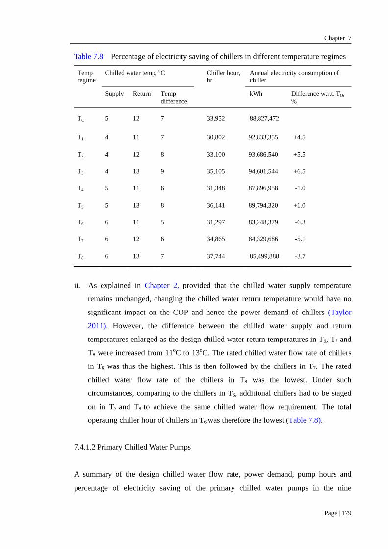
Chapter 7
Page | 179
Table 7.8 Percentage of electricity saving of chillers in different temperature regimes
Temp regime
Chilled water temp, oC Chiller hour, hr
Annual electricity consumption of chiller
Supply Return Temp difference
kWh Difference w.r.t. TO, %
TO 5 12 7 33,952 88,827,472
T1 4 11 7 30,802 92,833,355 +4.5
T2 4 12 8 33,100 93,686,540 +5.5
T3 4 13 9 35,105 94,601,544 +6.5
T4 5 11 6 31,348 87,896,958 -1.0
T5 5 13 8 36,141 89,794,320 +1.0
T6 6 11 5 31,297 83,248,379 -6.3
T7 6 12 6 34,865 84,329,686 -5.1
T8 6 13 7 37,744 85,499,888 -3.7
ii. As explained in Chapter 2, provided that the chilled water supply temperature
remains unchanged, changing the chilled water return temperature would have no
significant impact on the COP and hence the power demand of chillers (Taylor
2011). However, the difference between the chilled water supply and return
temperatures enlarged as the design chilled water return temperatures in T6, T7 and
T8 were increased from 11oC to 13oC. The rated chilled water flow rate of chillers
in T6 was thus the highest. This is then followed by the chillers in T7. The rated
chilled water flow rate of the chillers in T8 was the lowest. Under such
circumstances, comparing to the chillers in T6, additional chillers had to be staged
on in T7 and T8 to achieve the same chilled water flow requirement. The total
operating chiller hour of chillers in T6 was therefore the lowest (Table 7.8).
7.4.1.2 Primary Chilled Water Pumps
A summary of the design chilled water flow rate, power demand, pump hours and
percentage of electricity saving of the primary chilled water pumps in the nine

Chapter 7
Page | 180
temperature regimes is given in Table 7.9. In T6, the electricity consumption of the
primary chilled water pumps was the highest as it was 29.3% greater than that in the
base TO. On the other hand, the pumps in T3 had the lowest electricity consumption,
leading to a saving of 19.3% in comparison with those in TO.
Table 7.9 Percentage of electricity saving of the primary chilled water pumps in different temperature regimes
Temp regime
Chilled water temp, oC Design pump flow rate, l/s
Rated power, kW
Pump hour, hr
Annual electricity consumption of the pump
Supply Return Temp difference
kWh Difference w.r.t. TO, %
TO 5 12 7 718 164.4 33,952 5,583,218
T1 4 11 7 718 164.4 30,802 5,065,218 -9.3
T2 4 12 8 628 144.6 33,100 4,784,789 -14.3
T3 4 13 9 558 128.3 35,105 4,505,142 -19.3
T4 5 11 6 837 191.4 31,348 6,001,400 +7.5
T5 5 13 8 628 144.6 36,141 5,224,382 -6.4
T6 6 11 5 1,005 230.7 31,297 7,219,174 +29.3
T7 6 12 6 837 191.4 34,865 6,674,711 +19.5
T8 6 13 7 718 164.4 37,744 6,206,791 +11.2
These consumption patterns are the results of the relationship between the operating
frequency and the power demand of the pumps, which is explained below.
i. Primary chilled water pumps are interlocked with chillers to distribute chilled
water in the distribution loop. In this regard, the operating pump hours of the
primary pumps in the nine temperature regimes as shown in Table 7.9 were the
same as the corresponding operating chiller hours as shown in Table 7.8. As
shown in Table 7.9, despite of the long operating pump hours, the electricity
consumption of the pumps would not necessarily increase as it is also affected by
the power demand of the pumps.

Chapter 7
Page | 181
ii. The power demand of pumps also plays an important role in deciding the amount
of electricity they consume. A pump’s power demand depends on its design
pressure head and chilled water flow rate. As the chilled water pump
configurations were the same across all the temperature regimes, the pressure
head of the pumps should be the same. Therefore, the power demand is mainly
determined by the design chilled water flow rate, which is inversely proportional
to the temperature difference.
T3 was designed with the largest temperature difference, and hence the design
chilled water flow rate was the lowest. Accordingly, the power demand of the
pumps was the lowest in T3 (i.e. 128.3 kW), as shown in Table 7.9, but their
operating pump hours were also the highest. The energy simulation results show
that the pumps in T3 had the lowest electricity consumption. This implies that the
decrease in power demand could substantially offset the increase in the electricity
consumed by pumps even with the highest operating frequency.
7.4.1.3 Seawater Pumps
A summary of the design seawater flow rate, power demand, operating pump hours and
percentage of electricity saving of the seawater pumps is given in Table 7.10. The
electricity consumption of the seawater pumps in T8 was the highest, which was 10.9%
more than that in the base TO. On the contrary, the electricity consumption in T1 was the
lowest, as there was a saving of 9.1% in comparison with that in TO.
These consumption patterns reflect the relationship between the operating frequency
and power demand of the pumps, which is explained below.
i. Seawater pumps are also interlocked with chillers to circulate seawater for heat
dissipation. In this regard, the electricity consumption of seawater pumps is
determined by the operating frequency of chillers. In this study, the operating
pump hours of the seawater pumps of the nine temperature regimes as shown in
Table 7.10 were the same as the operating chiller hours of the corresponding
chillers as shown in Table 7.8.

Chapter 7
Page | 182
Table 7.10 Percentage of electricity saving of seawater pumps in different temperature regimes
Temp regime
Chilled water temp, oC Design pump flow rate, l/s
Rated power, kW
Pump hour, hr
Annual electricity consumption of the pump
Supply Return Temp difference
kWh Difference w.r.t. TO, %
TO 5 12 7 973 223.3 33,952 7,582,613
T1 4 11 7 975 223.9 30,802 6,896,226 -9.1
T2 4 12 8 975 223.9 33,100 7,410,722 -2.3
T3 4 13 9 975 223.9 35,105 7,859,620 +3.7
T4 5 11 6 973 223.3 31,348 7,001,053 -7.7
T5 5 13 8 973 223.3 36,141 8,071,490 +6.4
T6 6 11 5 971 222.9 31,297 6,975,753 -8.0
T7 6 12 6 971 222.9 34,865 7,771,021 +2.5
T8 6 13 7 971 222.9 37,744 8,412,718 +10.9
ii. The power demand of the seawater pump depends on its design pressure head and
seawater flow rate. As the seawater pumps’ configurations were the same in all the
temperature regimes, there was no change in the pressure head of the seawater
pumps. According to Equation 2.1 in Chapter 2, seawater flow rate is proportional
to the cooling capacity of chillers but is inversely proportional to the COP of
chillers. With the same cooling capacity of the chiller, the seawater pump’s design
flow rate decreased slightly as the COP of the chiller increased moderately when
the chilled water supply temperature was increased from 4oC to 6oC. In this regard,
the seawater pump’s power demand decreased accordingly.
Under such circumstances, it can be seen from Table 7.10 that the lower the
operating pump hours, the lower the electricity consumption of the seawater
pumps. The electricity consumption of the seawater pumps in T1 was the lowest.
This reflects that the operating pump hours of the pumps had a greater impact on
the seawater pump’s electricity consumption than their power demand.

Chapter 7
Page | 183
7.4.1.4 Overall Electricity Consumption of the Chiller Plant
Based on the electricity consumption data of the chillers, primary chilled water pumps
and seawater pumps in the nine design temperature regimes, a comparison of the total
electricity consumption of the chiller plant and the electricity savings in percentage is
given in Table 7.11.
Table 7.11 Percentage of electricity saving of the chiller plant in different temperature regimes
Temp regime
Chilled water temp, oC Annual electricity consumption of chiller plant
Supply Return Temp difference
kWh Difference w.r.t. TO, %
TO 5 12 7 101,993,303
T1 4 11 7 104,794,798 +2.7
T2 4 12 8 105,882,051 +3.8
T3 4 13 9 106,966,306 +4.8
T4 5 11 6 100,899,411 -1.1
T5 5 13 8 103,090,192 +1.1
T6 6 11 5 97,443,307 -4.6
T7 6 12 6 98,775,418 -3.2
T8 6 13 7 100,119,397 -1.8
The results indicate that the electricity consumption of the chiller plant was the highest
in T3 and the lowest in T6. In other words, T6 could save a maximum of 4.6% of
electricity in comparison with the base design TO.
7.4.2 Impacts of the Design Chilled Water Temperature on the Electricity
Consumption of Secondary Chilled Water Distribution Pumps
Keeping all other design aspects unchanged, any change in the temperature difference
between the design chilled water supply and return temperatures can lead to variations
in the secondary chilled water distribution pump’s design flow rates and hence the
power demand. The higher the temperature difference, the lower the design chilled
water flow rate.

Chapter 7
Page | 184
The pump’s design flow rate and power demand was the greatest when the design
temperature difference was the smallest, i.e. 5oC, as in T6. Moreover, the annual average
chilled water flow rate in T6 was also the highest. On the contrary, the least pump power
was required and the annual average chilled water flow rate was the lowest when the
design temperature difference was the greatest, i.e. 9oC, as in T3 (Table 7.12).
The percentage change in the electricity consumption of the secondary distribution
pumps in T1 to T8 exhibits the similar pattern of variation with that of the design pump
power and the annual average chilled water flow rate (see Table 7.12). The electricity
consumption of the pumps in T3 could save 20% of electricity in comparison with the
base case TO even though the operating pump hours were not the lowest.
Table 7.12 Percentage of electricity saving of the secondary chilled water distribution pumps in different temperature regimes
Temp regime
Chilled water temp, oC Design pump flow rate, l/s
Rated power, kW
Annual average chilled water flow rate, m3/s
Pump hour, hr
Annual electricity consumption of the secondary pump
Supply Return Temp difference
kWh Difference w.r.t. TO, %
TO 5 12 7 718 576.0 2.38 33,952 14,911,696
T1 4 11 7 718 576.0 2.15 30,802 13,333,416 -5.2
T2 4 12 8 628 481.2 2.03 33,100 12,342,376 -14.2
T3 4 13 9 558 423.7 1.93 35,105 11,857,991 -20.0
T4 5 11 6 837 709.4 2.53 31,348 15,944,134 +12.7
T5 5 13 8 628 481.2 2.25 36,141 13,766,463 -9.7
T6 6 11 5 1,005 920.2 2.92 31,297 18,367,820 +22.5
T7 6 12 6 837 709.4 2.84 34,865 18,065,505 +16.2
T8 6 13 7 718 576.0 2.69 37,744 17,054,325 +7.0
7.4.3 Overall Electricity Consumption of DCSO
As discussed in the previous sections, chiller plants and pumping stations exhibit
different electricity consumption patterns. With reference to Table 7.11, the chiller plant
designed with T6 had the lowest electricity consumption, which was 4.6% less than that

Chapter 7
Page | 185
in the base case TO. On the contrary, the secondary distribution pumps in the pumping
station designed with T3 had the lowest electricity consumption and could save 20% of
electricity with reference to TO (Table 7.12).
After summing up the electricity consumption figures of the chiller plant and the
secondary distribution pumps (Table 7.7), it was found that DCSO designed with the
chilled water supply and return temperatures of 6oC and 11oC respectively, i.e. in T6,
had the lowest electricity consumption. Nevertheless, when compared to the base design
TO, T6 could only lead to a saving of electricity by about 1%. This is because the gain in
electricity saving from the chiller plant was mostly offset by the increase in the
electricity consumption of the pumping stations.
7.5 Summary
Eight different temperature regimes, i.e. T1 to T8, were identified for comparing the
energy performance of different components in DCSO, where the design chilled water
supply and return temperatures were 5oC and 12oC respectively. It was found that in
temperature regime T6, in which the design chilled water supply and return temperatures
were 6oC and 11oC respectively, the annual total electricity consumption of DCSO was
the lowest.
Results further revealed that the chiller plant and pumping stations in T6 exhibited
different electricity consumption patterns. The energy performance of the chiller plant in
T6 was the best, leading to a saving of 4.6% in electricity when compared with other
temperature regimes. It is because the design chilled water supply temperature is on the
high side at 6oC. The COP was thus relatively higher as compared to other temperature
regimes with a design supply temperature of 4oC or 5oC.
On the other hand, it was found that the secondary distribution pumps in T6 had the
highest electricity consumption, as it was 22.5% higher with reference to the base
design TO. The reason is that when the design temperature difference was at the lowest
level, i.e. 5oC, this could lead to a higher annual average chilled water flow rate, and
hence a higher design pump power and electricity consumption of the pumps.

Chapter 7
Page | 186
Under such circumstances, the electricity saving of the chiller plant was nearly offset by
the increase in the electricity consumption of the secondary pumps. The overall
electricity consumption of DCSO could only be reduced by about 1% in comparison
with the base design TO.
In view of this, it was desirable to perform a comprehensive analysis of all the three
energy efficiency measures as mentioned in Chapters 5, 6 and 7, so as to identify an
integrated design solution for DCSO that could achieve an optimum energy performance
and the lowest life cycle cost.

Chapter 8
Page | 187
Chapter 8
A Techno-Economic Analysis of the Integrated Design
Solutions
8.1 Overview
Three energy efficiency enhancement measures were proposed in the preceding chapters
for mitigating the impacts of the degrading temperature difference on the energy
performance of DCSO. These measures include optimization of: (a) the chiller system
configuration; (b) the pumping station configuration; and (c) the chilled water
temperature.
By combining these three measures, a total of 1,447,680 combinations (options) of
design solutions could be generated. The present study focused on examining the energy
performance, financial viability and environmental benefit of these design solutions. In
view of the enormous number of combinations to be evaluated, a complete simulation
of all these options would take a prohibitively large amount of time and effort. In this
regard, a simple heuristic approach was developed to identify only those that possibly
are the optimal for analysis.
After identifying these possible solutions, the next step was to predict their electricity
consumptions by simulation for an evaluation of their energy performance. The results

Chapter 8
Page | 188
were then used for a comparison with the base design of DCSO. Regarding financial
viability, a life cycle cost (LCC) analysis of each possible solution was conducted to
find out the most cost-effective combination of chiller system configuration, pumping
station configuration and temperature regime. The environmental benefit, in respect of
reducing greenhouse gas emissions, by adopting the optimal design solution was also
estimated.
8.2 Simple Heuristic Strategy for Determining Possible Design Solutions
Based on the study results summarized in the preceding chapters, five combinations of
chiller system configurations, 36,192 arrangements of pumping station, and eight
temperature regimes were identified. The total number of combinations of these system
design options (= 5 x 36,192 x 8) equals 1,447,680. In view of this huge number of
options, a simple heuristic strategy was adopted to reduce the number for a detailed
analysis.
In this heuristic approach, only those combinations or arrangements that could lead to
the greatest reduction in the electricity consumption of DCSO were selected. These
“selected combinations or arrangements” were then combined to form a group of
“possible solutions”, which were then evaluated in terms of their energy performance,
financial viability and environmental benefits. The ultimate outcome would be an
“optimum design solution”, as illustrated in Figure 8.1.
8.2.1 Selection of Combinations of Chiller System Configuration
The different combinations of chiller system configuration and the amount of annual
total electricity saving with reference to the base design CO are shown in Table 8.1. The
results indicate that among the five combinations, CA, CD and CE could lead to a 10%,
11% and 11.6% reduction in electricity consumption, respectively, which were
significantly higher than those of CB and CC. Therefore, CB and CC were not further
considered in the next stage of analysis.

Chapter 8
Page | 189
Figure 8.1 Elimination process of achieving an optimum design solution
Table 8.1 Percentage of annual electricity saving with different chiller system configurations
Chiller system configuration
No. of chiller
Size Type Annual electricity consumption of DCSO
kWh Difference w.r.t. CO, %
CO 10 Equal Constant speed 116,904,999
CA 10 Equal Variable speed 105,294,444 -9.9
CB 15 Equal Constant speed 115,005,198 -1.6
CC 15 Unequal Constant speed 113,484,601 -2.9
CD 15 Equal Variable speed 104,105,583 -10.9
CE 15 Unequal Variable speed 103,295,586 -11.6
8.2.2 Selection of Pumping Station Arrangement
For the 36,192 pumping station arrangements, their annual total electricity
consumptions were compared with those of the base case PS1-0 (Table 2.7 in Chapter 2).
Table 8.2 shows the average percentage of the difference of the annual total electricity
consumption. Only three arrangements where a single pumping station was used were

Chapter 8
Page | 190
unable to reduce the electricity consumption of DCSO. As a result, a total of 36,189
arrangements were retained for analysis at the next stage.
Table 8.2 Percentage of annual total electricity saving with different pumping station arrangements
No. of pumping station
Total no. of arrangement
% of total no. of arrangement
Average % of difference w.r.t. base PS1-0
1 3 0.01 +0.12
2 63 0.17 -0.85
3 567 1.57 -1.44
4 2,997 8.28 -1.78
5 10,692 29.54 -2.04
6 21,870 60.43 -2.22
36,192 100
8.2.3 Selection of Chilled Water Temperature Regime
Regarding chilled water temperature, only four temperature regimes, i.e. T4, T5, T6 and
T7, could lead to a reduction in the annual total electricity consumption of DCSO (see
Table 8.3). Hence, these four temperature regimes were further analyzed in conjunction
with the other selected options.
Table 8.3 Percentage of annual electricity saving in different temperature regimes
Temp regime
Chilled water temp, oC Annual electricity consumption of DCSO
Supply Return Delta-T kWh Difference w.r.t. TO, %
TO 5 12 7 116,904,999
T1 4 11 7 118,128,214 +1.05
T2 4 12 8 118,224,427 +1.13
T3 4 13 9 118,824,297 +1.64
T4 5 11 6 116,843,545 -0.05
T5 5 13 8 116,856,655 -0.04
T6 6 11 5 115,811,127 -0.94
T7 6 12 6 116,840,923 -0.05
T8 6 13 7 117,173,722 +0.23

Chapter 8
Page | 191
After the elimination process, the number of possible solutions was substantially
reduced by 70% from 1,447,680 (= 5 x 36,192 x 8) to 434,268 (= 3 x 36,189 x 4).
These 434,268 possible solutions can be expressed by the matrix S(Ci,Tj,PSnps-x) to
represent a mixture of the three energy efficiency enhancement measures, where Ci
represents one of the three selected combinations of chiller system configuration, Tj one
of the four selected temperature regimes, and PSnps-x one of the 36,189 pumping station
arrangements, where nps is the number of pumping station (i.e. 1 to 6) and x the number
of arrangement from 1 to 36,189.
The following are the matrices of the 434,268 possible design solutions.
S(CA,T4,PS1-1), S(CA,T4,PS1-2), S(CA,T4,PS2-3), …, S(CA,T4,PS6-36189)
S(CA,T5,PS1-1), S(CA,T5,PS1-2), S(CA,T5,PS2-3), …, S(CA,T5,PS6-36189)
S(CA,T6,PS1-1), S(CA,T6,PS1-2), S(CA,T6,PS2-3), …, S(CA,T6,PS6-36189)
S(CA,T7,PS1-1), S(CA,T7,PS1-2), S(CA,T7,PS2-3), …, S(CA,T7,PS6-36189)
S(CD,T4,PS1-1), S(CD,T4,PS1-2), S(CD,T4,PS2-3), …, S(CD,T4,PS6-36189)
S(CD,T5,PS1-1), S(CD,T5,PS1-2), S(CD,T5,PS2-3), …, S(CD,T5,PS6-36189)
S(CD,T6,PS1-1), S(CD,T6,PS1-2), S(CD,T6,PS2-3), …, S(CD,T6,PS6-36189)
S(CD,T7,PS1-1), S(CD,T7,PS1-2), S(CD,T7,PS2-3), …, S(CD,T7,PS6-36189)
S(CE,T4,PS1-1), S(CE,T4,PS1-2), S(CE,T4,PS1-3), …, S(CE,T4,PS6-36189)
S(CE,T5,PS1-1), S(CE,T5,PS1-2), S(CE,T5,PS1-3), …, S(CE,T5,PS6-36189)
S(CE,T6,PS1-1), S(CE,T6,PS1-2), S(CE,T6,PS1-3), …, S(CE,T6,PS6-36189)
S(CE,T7,PS1-1), S(CE,T7,PS1-2), S(CE,T7,PS1-3), …, S(CE,T7,PS6-36189)
8.3 Simulation of Energy, Financial and Environmental Performances
To evaluate the performance of these 434,268 possible solutions in the captioned three
aspects, the first step was to simulate their electricity consumption patterns. Then it was
necessary to collect their capital and operation cost data for calculating their LCC. This
allowed a cost-optimal solution that could lead to the lowest LCC to be identified.

Chapter 8
Page | 192
Based on the simulated electricity consumption figures, environmental benefits of the
most cost-effective solution, in terms of reduction of CO2 emissions, could be
determined.
8.3.1 Simulation of Electricity Consumption and CO2 Emissions
Figure 8.2 shows the algorithm used to predict the electricity consumption of the
possible solutions. Before conducting the simulation, the first step was to define the
temperature regime, Tj, as this would affect both the energy performance of the chiller
system and pumps in a specific pumping station configuration. Then, the electricity
consumption of chiller system configurations CA, CD and CE, and the 36,189 pumping
station arrangements under temperature regimes T4, T5, T6 and T7 were simulated
according to the chiller plant model and pumping station model developed in Chapters 3
and 6 respectively.
The electricity consumption of any possible solution equals the summation of the
electricity consumption of the chiller plant and pumping station under the same
temperature regime.
In order to perform the simulation in a more efficient manner, a program written in VBA
was established to integrate the mathematical models of the chiller plant and pumping
station and calculate the annual total electricity consumption of all possible solutions.
Regarding CO2 emissions, it could be estimated from the energy consumption of each
possible solution, based on the CO2 emissions factor of 197 tonnes of CO2 (equivalent)
emissions per TJ of electricity demand (Yik et al., 2012).

Chapter 8
Page | 193
Figure 8.2 Algorithm of identifying an energy-optimal design solution with the
lowest electricity consumption
8.3.2 The LCC Model
The life cycle cost analysis deployed in this thesis is built upon the LCC approach
developed by Fuller and Petersen (1996), where is structured approach to address all the
different costs of a project over a given study period with all the potential cost adjusted
to reflect the time-value of money. An LCC analysis was performed to examine all the
different costs of a DCS over a given study period. All potential costs were adjusted to
reflect the time-value of money. After discounting or reducing all costs to current values
or converting them into an annual cost, the LCC model was used to determine a
cost-optimal design solution out of a set of possible design solutions as mentioned in
Section 8.2. Within the range of possible design solutions, solutions with a lower LCC
would be more financially favourable than those with a higher LCC. This information
can provide a good reference for the DCS designers or owners in deciding whether or
not to adopt a particular solution from a financial viability point of view.

Chapter 8
Page | 194
8.3.2.1 LCC Analysis Estimation
In this study, the useful life span of a DCS was set to be 60 years. The life spans of
chillers, chilled water and seawater pumps would be much shorter. The assumed life
spans of all equipment and the number of times that they would require to be replaced
within the life span of the DCS are summarized in Table 8.4.
Table 8.4 Life span and number of replacement of equipment
Life span, year No. of replacement
Direct seawater-cooled chiller (constant/variable speed) 30 2
Primary chilled water pump (constant speed) 20 3
Secondary chilled water pump (variable speed) 20 3
Seawater pump (constant speed) 15 4
The reasons for adopting 60 years as the analysis period are as follows.
i. The typical design service life for long life buildings, including offices and
commercial buildings, is 50 to 99 years (Hovde and Moser, 2004). The 60-year
life span of a DCS is within this range.
ii. The various types of equipment, as listed in Table 8.4, had different life spans,
and their replacement would take place at different points in time within the life
span of the DCS, whilst 60 years is the least common multiple of the life span of
the equipment involved.
As a result, taking 60 years as the lifespan of a DCS could provide an equal basis for a
fair comparison among the equipment. Otherwise, the LCC estimation could be unduly
increased because the pumps would remain usable by the end of the life span covered
by the analysis. In this case, such equipment would be regarded as being disposed of
before they could be due for replacement.
The LCC of the DCS in this study was calculated based on the following assumptions.

Chapter 8
Page | 195
i. All the equipment is a new establishment.
ii. All monetary values are in constant Hong Kong dollars (i.e. already adjusted with
inflation factor).
iii. The price of electricity is $1/kWh, which was assumed to rise steadily at a real
escalation rate of 2% per annum, and the real discount was taken to be 5% per
annum (Yik et al., 2012).
iv. A DCS operator has to pay the annual licensing fee for laying chilled water
distribution pipes on government land. According to a consultancy study
conducted in 1999, the unit rate has been HK$13 per 10 mm diameter per meter
run (EMSD, 1999). It was anticipated that the government would adjust the unit
rate periodically, but not frequently. For simplicity of estimation, the unit rate was
assumed to increase with the inflation rate. As shown in Figure 8.3, the unit rate in
2013 was HK$14.85 per 10 mm diameter per meter run.
v. The replacement cost of the equipment listed in Table 8.4 is the same as the initial
cost in constant dollars. The life span of such equipment (Wong and Tang, 2010;
Yik et al., 2012), as shown in Table 8.4, can be used to determine the present
value of replacement cost.
vi. The annual maintenance cost is 1.5% of the initial capital cost (Anagnostopoulos
and Papantonis, 2007).

Chapter 8
Page | 196
Figure 8.3 Monthly average inflation rate, 2000-2013 (Source: Trading Economics, 2013)
vii. The land cost that the Hong Kong government calculated for the DCS plant or
pump house at the Kai Tak Development was based on the accommodation value,
which is defined as the land value per the gross floor area to be built on site for
the plant or pump house, including the basement. The accommodation value for
that DCS has been taken at HK$1,500 per m2 (EMSD, 2003c). This value is far
below the market accommodation value because the land was restricted to be a
government, institution or community site for new development. As no empirical
data or formula was available for estimating or predicting this strategic land cost
of DCSO, the accommodation value used for the Kai Tak Development was
adopted for the present study.
8.3.2.2 Capital Cost
Capital costs refer to the costs of the major equipment in this study. This major
equipment included the constant and variable speed direct seawater-cooled chillers,
primary constant speed chilled water and seawater pumps, and secondary variable speed
chilled water distribution pumps. Their cost data was obtained from the local market.

Chapter 8
Page | 197
i. Chillers
Table 8.5 is a summary of the unit costs of the supply and installation of constant and
variable speed chillers with different cooling capacities and associated accessories.
Moreover, the land cost of installing the chiller in the chiller plant room is taken into
account. Based on the accommodation value assumed in Section 8.3.2.1, gross floor
area (GFA) required for installing the chiller was estimated and the land cost per the
cooling capacity of chiller was calculated, as shown in Table 8.5.
Table 8.5 Different costs of the constant speed and variable speed chillers
Constant speed chiller Variable speed chiller
Cooling capacity, RT/kW 2,000 /
7,034
4,000 /
14,068
6,000 /
21,102
2,000 /
7,034
4,000 /
14,068
6,000 /
21,102
Chiller and accessories cost, HK$/RT
3,000 3,500 4,000 3,900 4,550 5,200
Installation cost, HK$/RT 3,900 4,550 5,200 5,070 5,915 6,760
Land cost, HK$/RT 12 9 8 12 9 8
Total unit cost, HK$/RT 6,912 8,059 9,208 8,982 10,474 11,968
ii. Secondary variable speed chilled water distribution pumps
The capital cost of a chilled water distribution pump set consists of the cost of variable
speed pumps, variable speed drives, motors, pipework, land and fittings and installation.
As presented in Chapter 6, thousands of pumps could be involved in the simulation
process and this would require a prohibitively large amount of time and effort to obtain
the cost data of each pump. In this regard, the capital cost data of 16 chilled water
distribution pump sets with different capacities was obtained from the manufacturers
(see Table 8.6).

Chapter 8
Page | 198
Table 8.6 Capital costs of variable speed chilled water pumps with different operational characteristics
Flow rate, m3/s
Pressure head, bar
Rated Power, kW
Cost, HK$
Pump and motor
Variable speed drive
Pipework Land cost
Total cost Unit cost per kW
1 0.36 0.70 36 450,000 12,750 18,860 9,186 490,796 13,752
2 0.29 1.03 41 480,000 17,400 16,000 9,891 523,291 12,627
3 0.27 1.21 46 480,000 17,400 16,000 9,891 523,291 11,485
4 0.58 0.55 54 500,000 22,680 28,000 13,154 563,834 10,438
5 0.40 1.21 68 550,000 22,680 22,000 13,721 608,401 8,937
6 0.36 2.25 116 650,000 26,600 18,860 14,765 710,225 6,142
7 0.80 1.21 138 700,000 42,100 36,000 18,118 796,218 5,760
8 0.54 2.25 173 780,000 48,100 24,460 16,173 868,733 5,028
9 1.09 1.70 261 1,000,000 66,970 60,000 19,737 1,146,707 4,398
10 0.46 4.42 291 1,250,000 88,200 22,000 16,173 1,376,373 4,735
11 0.46 6.10 410 1,600,000 95,900 22,000 18,450 1,736,350 4,231
12 1.09 2.73 420 1,800,000 150,000 60,000 19,737 2,029,737 4,832
13 0.69 4.42 431 1,600,000 155,760 32,340 20,032 1,808,132 4,200
14 0.69 6.10 589 1,900,000 212,800 32,340 19,500 2,164,640 3,675
15 1.38 4.42 862 2,500,000 320,000 100,000 20,158 2,940,158 3,410
16 1.38 6.10 1185 3,500,000 450,000 100,000 20,158 4,070,158 3,435
Figure 8.4 shows the relationship of their total capital costs over their pump power. A
trend line was plotted. The unit cost is relatively high for a small scale pump set. It
decreases to a minimum value with the increase in pump power, upholding the principle
of economies of scale. The pump cost can be described by Equation 8.1.
Costcwp, var = 51,123 x Wcwp, var-0.411 (8.1)
where
Costcwp,var = Unit cost of a variable speed chilled water pump (HK$ per
kW)
Wcwp,var = Pump power of a variable speed chilled water pump (kW)

Chapter 8
Page | 199
Figure 8.4 Unit cost of the variable speed pump set per pump power
iii. Primary constant speed chilled water and seawater pumps
The above methodology used for estimating the costs of the variable speed chilled water
pump was applied for developing the cost models for the constant speed primary chilled
water pumps and seawater pumps. Based on the cost data provided by the
manufacturers and contractors, Equations 8.2 and 8.3 can be used for determining the
costs of a constant speed chilled water pump set and a seawater pump set respectively.
Costcwp, const = 39,775 x W cwp, const-0.407 (8.2)
Costswp, const = 59,138 x Wswp, const-0.413 (8.3)
where
Costcwp, const = Unit cost of a constant speed chilled water pump, HK$ per kW
Wcwp, const = Pump power of a constant speed chilled water pump, kW
Costswp, const = Unit cost of a constant speed seawater water pump, HK$ per kW
Wswp, const = Pump power of a constant speed seawater water pump, kW

Chapter 8
Page | 200
8.3.2.3 Operating Expenses
Operating expenses include the replacement cost, the annual electricity cost, the annual
license fee for laying chilled water distribution pipes on government land, and the
annual maintenance cost.
i. Electricity Cost
The life-cycle electricity cost, LCC(E), in present value is determined on the basis of the
recurrent annual electricity cost, C(E), using Equation 8.4.
EUSPWFECELCC )()( (8.4)
where
ii. License Fee
The life-cycle license cost, LCC(L), in present value is determined on the basis of the
recurrent annual license cost, C(L ), for laying the pipework, using Equation 8.5.
LUSPWFLCLLCC )()( (8.5)
where
USPWFL = DCS
DCS
LS
LS
dd
d
)1(
1)1(
USPWFE =
DCSLS
d
e
ed
e
1
11
)(
)1(
d = real discount rate, % per annum
e = real escalation rate of electricity price, % per annum
LSDCS = useful life span of a DCS, in years
Remark: USPWF - Uniform series present worth factor

Chapter 8
Page | 201
iii. Maintenance Cost
The maintenance cost covered the costs of regular check-up and system overhaul. The
life-cycle maintenance cost, LCC(M), in present value is derived from the recurrent
annual maintenance cost, C(M), using Equation 8.6.
MUSPWFMCMLCC )()( (8.6)
where
USPWFM = DCS
DCS
LS
LS
dd
d
)1(
1)1(
iv. Replacement Cost
The life cycle cost of replacement is the present value of the total replacement cost of
equipment, PV(CostTR), throughout its life span in the DCS (Table 8.5). It can be
determined by Equation 8.7.
R
e
N
iLSi
RTR
d
CostCostPV
1 )1()( (8.7)
where
NR = number of times of replacement
CostR = replacement cost of equipment
LSe = useful life of equipment, in years
8.3.2.4 Overall LCC
After each cost component was derived, the present values of electricity, license,
maintenance, replacement and capital costs over the 60-year period were summed up to
determine the total LCC of all the possible solutions by Equation 8.8.
TRCostPVMLCCLLCCELCCCostCapitalLCC )( )( )( (8.8)

Chapter 8
Page | 202
8.4 An LCC Analysis of All Possible Solutions
8.4.1 Comparison of the LCC of all possible design solutions with DCSO
In order to evaluate the cost-effectiveness of various possible solutions, it was necessary
to predict the capital cost for investment and the total operating cost the solutions could
save. This information was important because operating costs are typically greater than
capital costs (Yates, 2011).
Tables 8.7, 8.8 and 8.9 show a comparison of the average LCC saving of all the 434,268
possible design solutions identified in Section 8.2 with reference to the LCC of the base
case DCSO using the three energy efficiency enhancement measures selected in Section
8.2.
Among the three selected chiller system configuration options such as CA, CD and CE,
the average LCC saving of the solutions designed with CD was the highest, i.e. 5.71%.
The configuration of CD consisted of 15 equally-sized variable speed chillers.
Regarding the use of two to six pumping station options as shown in Table 8.8, the
solutions designed with six pumping stations as in P6 had achieved the highest average
LCC saving, i.e. 4.17%, in comparison with other options.
On the other hand, under temperature regime T5 where the chilled water supply and
return temperatures were at 5oC and 13oC respectively (Table 8.9), the highest average
LCC saving of 4.92% was achieved.

Chapter 8
Page | 203
Table 8.7 Percentage of average LCC saving of the solutions designed with chiller system configurations CA, CD and CE with reference to DCSO
Chiller system configuration
No. of design solution
Total % of LCC saving, HK$
Average LCC saving w.r.t. to base DCSO, %
CA 144,756 233,106 1.61
CD 144,756 825,967 5.71
CE 144,756 729,502 5.04
Table 8.8 Percentage of average LCC saving of the solutions designed with different number of pumping stations with reference to DCSO
No. of pumping station
No. of design solution
Total % of LCC saving, HK$
Average LCC saving w.r.t. to base DCSO, %
2 PS 756 2,600 3.44
3 PS 6,804 25,834 3.80
4 PS 35,964 142,475 3.96
5 PS 128,304 523,683 4.08
6 PS 262,440 1,093,883 4.17
Table 8.9 Percentage of average LCC saving of the solutions designed with temperature regimes T4, T5, T6 and T7 with reference to DCSO
Temperature regime No. of design solution
Total % of LCC saving, HK$
Average LCC saving w.r.t. to base DCSO, %
T4 108,567 355,969 3.28
T5 108,567 534,435 4.92
T6 108,567 406,516 3.74
T7 108,567 491,556 4.53
8.4.2 A Cost-Optimal Design Solution
The LCC savings of the 434,268 design solutions as a result of adopting different
combinations of the three energy efficiency measures were summarized in Table 8.10.
The solutions were ranked according to the percentage of LCC saving they could
achieve in comparison with the base DCSO.

Chapter 8
Page | 204
Table 8.10 Ranking of the 434,268 design solutions based on the LCC saving achieved in comparison with DCSO
Ranking (from highest LCC saving achieved w.r.t to base DCSO)
No. of solution
Chiller system configuration (% in the ranking group)
Temperature regime (% in the ranking group)
No. of pumping station (PS) (% in the ranking group)
LCC saving (=S), %
1 (Solution C) 1
CD (100%) T5 (100%) 6 PS (100%) S = 7.50
2 to 6 5 CD (100%) T5 (100%) 6 PS (100%)
7.46 ≤ S < 7.5
7 to 578 572 CD (100%) T5 (100%) 6 PS (68%) 5 PS (28%) 4 PS (4%)
7.21 ≤ S < 7.46
579 to 10,337 9,759 CD (100%) T5 (91%) T7 (9%)
6 PS (68%) 5 PS (26%) 4 PS (6%)
6.82 ≤ S < 7.21
10,338 to 289,168 278,831 CD (48%) CE (52%)
T4 (26%) T5 (22%) T6 (26%) T7 (26%)
6 PS (60%) 5 PS (30%) 4 PS (8%) 3 PS (2%)
3.15 ≤ S < 6.82
289,169 to 433,615 144,447 CA (100%) T4 (25%) T5 (25%) T6 (25%) T7 (25%)
6 PS (60%) 5 PS (30%) 4 PS (8%) 3 PS (2%)
0 < S < 3.15
433,616 to 434,268 653 CA (100%) T4 (86%) T6 (14%)
6 PS (42%) 5 PS (22%) 4 PS (22%) 3 PS (10%) 2 PS (4%)
-1 < S < 0
After comparing the LCC of all the 434,268 possible solutions with that of DCSO, it was
found that matrix S(CD,T5,PS6-34735) (henceforth referred to as “Solution C”) had the
lowest LCC, i.e. HK$4,108,032,442, which was about 7.5% lower than that of DCSO.
This cost-optimal design consisted of 15 x 4,000 RT (14,068 kW) variable speed
chillers and six pumping stations with five pumps in each station. The design chilled
water supply and return temperatures were 5oC and 13oC respectively. It was found that
the system features of Solution C, i.e. the chiller system configuration, the number of
pumping station and the temperature regime, were identical with the designs of the three
solutions with the highest average LCC saving, as identified in Section 8.4.1 where the
comparison was based on each individual measure. Table 8.11 provides a comparison of
the system details of DCSO and Solution C.

Chapter 8
Page | 205
Table 8.11 Comparison of the system details of DCSO and Solution C
DCSO Solution C
1. Chiller system configuration CO CD
Total no. 10 15
Nominal cooling capacity per chiller, RT/kW 6,000 / 21,102 4,000 / 14,068
Constant/variable speed Constant Variable
2. Pumping station configuration PS1-0 PS6-34735
No. of pumping station 1 6
No. of pump in each station 10 5
Location of pumping station 1 on supply side 5 on supply side 1 on return side
3. Temperature regime TO T5
Chilled water supply temp, oC 5 5
Chilled water return temp, oC 12 13
Delta-T, oC 7 8
The LCC saving of five solutions (i.e. the 2nd to the 6th) was in the range of 7.46% to
7.5%, which was close to the LCC saving of Solution C. The matrices of these solutions
were more or less the same as Solution C’s except that the six pumping stations were
arranged in different locations.
The third group was the 572 solutions (ranked 7th to 578th) that had an LCC saving
between 7.21% and 7.46%. These solutions also adopted CD and T5 as the chiller system
configuration and temperature regime respectively. However, their number of pumping
station was not identical, as 68% of them were of a six-pumping station design while
the remaining were designed with four or five pumping stations.
The fourth group consisted of 9,759 solutions that were also designed with chiller
system configuration CD. Concerning temperature regime and number of pumping
station, the use of T5 and six pumping stations was still a dominant feature.
As a result, it can be concluded that chiller system configuration CD, temperature
regime T5 and the use of six pumping stations are the most critical factors for achieving
a low LCC.

Chapter 8
Page | 206
Despite of its lowest LCC, however, the total annual electricity consumption of Solution
C was not the lowest. The most energy-optimal design solution that could lead to the
lowest electricity consumption (henceforth referred to as “Solution E”) was matrix
S(CE,T7,PS6-35464). It consisted of 15 unequally-sized (i.e. 5 x 2,000 RT (7,034 kW), 5 x
4,000 RT (14,068 kW) and 5 x 6,000 RT (21,102 kW)) variable speed chillers and six
pumping stations with five pumps in each station. The design chilled water supply and
return temperatures were 6oC and 12oC, respectively. The annual electricity
consumption of using the base design DCSO was 116,904,999 kWh. After the adoption
of Solution E, however, the annual electricity consumption was reduced by 15.3% to
99,035,646 kWh.
Compared to Solution E, the electricity consumption of Solution C was slightly higher,
i.e. ~1%, as shown in Table 8.12. This difference, however, is insignificant because it
was mainly due to the relative high electricity consumption of chillers, which could not
be compensated by the electricity saving of the secondary chilled water pumps.
Table 8.12 Comparison of the annual electricity consumption of Solutions C and E
Annual electricity consumption, kWh Difference [Solution C minus Solution E]
Solution C Solution E kWh %
(a) Chiller plant
i. Chiller 76,555,222 71,966,990 +4,588,233 +6.4
ii. Pri. ch. w. pumps 4,958,662 6,071,321 -1,112,659 -18.3
iii. Seawater pump 7,675,345 7,058,226 +617,119 +8.7
Total [i + ii + iii] 89,189,230 85,096,537 +4,092,692 +4.8
(b) Sec. ch. w. pumps 10,696,493 13,939,109 -3,242,616 -23.3
Total [(a) + (b)] 99,885,723 99,035,646 850,076 +0.9
Table 8.13 is a summary of the LCC of capital investment, license, replacement,
maintenance, and energy of both Solutions C and E. The result indicates that the LCC of
Solution C was lower than that of Solution E and is hence more financially viable.

Chapter 8
Page | 207
Table 8.13 Comparison of the LCC of Solutions C and E
Solution C Solution E
(a) Total initial capital investment, HK$ 676,894,270 713,379,294
(b) Life-cycle replacement cost, HK$ 357,645,409 376,439,378
(c) Life-cycle maintenance cost, HK$ 192,196,914 202,556,448
(d) Life-cycle license cost, HK$ 117,124,979 117,124,979
(e) Life-cycle energy cost, HK$ 2,764,170,870 2,738,956,176
Total LCC, HK$ 4,108,032,442 4,148,456,275
8.4.3 A Comparative Analysis of the LCC of DCSO and Solution C
A detailed comparison of the different costs and overall LCC of DCSO and Solution C is
given in Table 8.14. It can be seen that the present value LCC of Solution C was
HK$332 million less than that of DCSO, representing a saving of 7.5%.
For Solution C, the adoption of energy efficiency enhancement measures such as using
variable speed chillers, and operating more chillers and pumps to achieve a higher
energy performance could lead to a 13.2% increase in its LCC of capital investment.
More specifically, the use of variable speed chillers accounted for the largest portion, i.e.
~96%, of the additional capital cost.
On the contrary, regarding pumping stations, the use of six pumping stations and less
secondary pumps in each station could save 2.3% of the capital cost as compared to the
use of a single pumping station and more pumps in each station in DCSO. In the
estimation, account had also been taken into about the associated higher maintenance
and replacement costs, which were incurred by the greater amount of equipment to be
maintained and replaced. The total LCC of Solution C in terms of the costs of capital
investment, maintenance and replacement was 13.2% higher than that of DCSO.

Chapter 8
Page | 208
Table 8.14 Comparison of the LCC of DCSO and Solution C
LCC, HK$ Difference in LCC [Solution C minus DCSO]
DCSO Solution C HK$ %
(a) Total initial capital investment
i. Chiller 552,480,000 628,440,000 +75,960,000 +13.7
ii. Pri. ch. w. pumps 8,726,948 9,533,092 +806,144 +9.2
iii. Seawater pump 15,050,744 17,809,998 +2,759,254 +18.3
iv. Sec. ch. w. pumps 21,605,376 21,111,180 -494,196 -2.3
Sub-total 597,863,068 676,894,270 +79,031,202 +13.2
(b) Life-cycle replacement cost
i. Chiller 286,701,300 326,119,615 +39,418,315 +13.7
ii. Pri. ch. w. pumps 4,528,720 4,947,057 +418,336 +9.2
iii. Seawater pump 13,202,913 15,623,404 +2,420,491 +18.3
iv. Sec. ch. w. pumps 11,211,789 10,955,334 -256,456 -2.3
Sub-total 315,644,723 357,645,409 +42,000,687 +13.3
(c) Life-cycle maintenance cost
i. Chiller 156,870,808 178,438,841 +21,568,032 +13.7
ii. Pri. ch. w. pumps 2,477,924 2,706,820 +228,896 +9.2
iii. Seawater pump 4,273,498 5,056,959 +783,461 +18.3
iv. Sec. ch. w. pumps 6,134,616 5,994,295 -140,322 -2.3
Sub-total 169,756,847 192,196,914 +22,440,067 +13.2
(d) Life-cycle license cost 117,124,979 117,124,979 0 0
(e) Life-cycle energy cost
i. Chiller 2,489,642,370 2,145,677,686 -343,964,684 -13.8
ii. Pri. ch. w. pumps 140,836,992 125,082,536 -15,754,456 -11.2
iii. Seawater pump 191,271,861 193,611,031 +2,339,170 +1.2
iv. Sec. ch. w. pumps 417,942,662 299,799,617 -118,143,044 -28.3
Sub-total 3,239,693,884 2,764,170,870 -475,523,014 -14.7
Total LCC 4,440,083,501 4,108,032,442 -332,051,058 -7.5
Despite of the higher capital investment, and life-cycle replacement and maintenance
costs of Solution C, its total life-cycle energy cost was 14.7% less than that of DCSO.
75% of the saving is attributed by the chiller plant, which used 15 x 4,000 RT (14,068
kW) equally-sized variable speed chillers. The remaining saving of 25% was generated

Chapter 8
Page | 209
by the pumping stations. This revealed that although additional costs were required for
the equipment and energy efficiency enhancement measures in Solution C, the life-cycle
energy cost saving achieved is more than enough to offset the extra costs incurred.
8.5 A Comparative Analysis of the Electricity Consumption of DCSO and
Solution C
Results from energy simulation (as in Table 8.15) show that when DCSO adopted the
design of Solution C, its annual total electricity consumption could be reduced by
14.6%.
Over 72 % of this saving in electricity was generated by the chillers, i.e. the 15 x 4,000
RT (14,068 kW) chillers. It is then followed by the application of six pumping stations
with five pumps in each station. These secondary chilled water pumps were responsible
for 25% of the total reduction in electricity consumption. Some observations can be
made about the simulation results.
Table 8.15 Comparison of the annual electricity consumption of DCSO and Solution C
Annual electricity consumption, kWh
Difference [Solution C minus DCSO]
% of the total difference
DCSO Solution C kWh %
(a) Chiller plant
i. Chiller 88,827,472 76,555,222 -12,272,250 -13.8 72
ii. Pri. ch. w. pumps 5,583,218 4,958,662 -624,556 -11.2 3
iii. Seawater pump 7,582,613 7,675,345 +92,732 +1.2 0
Total [i + ii + iii] 101,993,303 89,189,230 -12,804,074 -12.6 75
(b) Sec. ch. w. pumps 14,911,696 10,696,493 -4,215,203 -28.3 25
Total [(a) + (b)] 116,904,999 99,885,723 -17,019,276 -14.6

Chapter 8
Page | 210
8.5.1 Electricity Consumption of Chillers
The adoption of additional and smaller sized variable speed chillers in Solution C could
bring a significant reduction of 13.8% in electricity consumption in comparison with the
use of less and larger sized constant speed chillers in DCSO (see Table 8.15). The main
reason is that the COP of variable speed chillers is relatively higher than that of constant
speed chillers, particularly at low load. This has already been discussed in Chapter 6.
Furthermore, as there were 77% of the system’s total operating hours (c.f. Table 2.5 in
Chapter 2) in which the system load was below 50%, it means that the chillers were
operated at part load for most of the time. Under such circumstances, the variable speed
chillers could help to significantly reduce the electricity consumption of DCSO.
Figure 8.5 shows that the average COP of the variable speed chillers in CD of Solution C
was relatively high at low load when compared to that in CO of DCSO. The average COP
of constant speed chillers decreased dramatically at low load. More specifically, the
annual average COP of the chiller system configuration in Solution C was 7.43, which
was relatively higher than that of DCSO, i.e. 5.69.
Figure 8.5 Average COP of the constant and variable speed chillers in CO and CD that
are operating at different PLR

Chapter 8
Page | 211
8.5.2 Electricity Consumption of Primary Chilled Water Pumps
Similar to chillers, the electricity consumption of the primary chilled water pumps in
Solution C was also relatively lower than that in DCSO, as there was a 11.2% difference
between them (see Table 8.16).
Table 8.16 Comparison of the operating pump hour, power demand and electricity consumption of the primary chilled water pumps in DCSO and Solution C
DCSO Solution C
No. of chiller 10 15
Cooling capacity of chiller, RT/kW 6,000 / 21,102 4,000 / 14,068
Operating pump hour, hr 33,952 51,474
No. of pri. ch. w. pump 10 15
Rated power, kW 164.4 96.3
Total power demand, kW 1,644 1,445
Annual electricity consumption, kWh 5,583,218 4,958,662
Difference in annual electricity consumption w.r.t. DCSO
kWh - -624,556
% - -11.2
Their electricity consumptions depend on their power demand and operating pump hour,
as in Table 8.16. Under the same pressure head requirement, the design delta-T in
Solution C (i.e. 8oC) was relatively higher than that of DCSO (i.e. 7oC). This led to a
lower design flow rate and power demand of the primary chilled water pumps in
Solution C. Although the operating pump hours of the pumps in Solution C were
relatively longer, the low power demand of the pumps there had led to a lower
electricity consumption.

Chapter 8
Page | 212
8.5.3 Electricity Consumption of Seawater Pumps
Same as the primary chilled water pumps, the electricity consumption of the seawater
pumps also depends on the pump’s power demand and operating pump hour. The
electricity consumption of the seawater pumps in Solution C was 1.2% higher than that
in DCSO (Table 8.17). However, as seawater pumps accounted for only a small portion
of the total electricity consumption of DCSO, this additional electricity consumption was
offset by the significant savings derived from the chillers and secondary chilled water
pumps.
Table 8.17 Comparison of power demand and electricity consumption of the seawater pumps in DCSO and Solution C
DCSO Solution C
No. of chiller 10 15
Cooling capacity of chiller, RT / kW 6,000 / 21,102 4,000 / 14,068
Operating pump hour, hr 33,952 51,474
No. of seawater pump 10 15
Rated pump power, kW 223.3 149.1
Total power demand, kW 2,233 2,237
Annual electricity consumption, kWh 7,582,613 7,675,345
Difference in annual electricity consumption w.r.t. DCSO
kWh - +92,732
% - +1.2
8.5.4 Electricity Consumption of Secondary Chilled Water Pumps
Table 8.18 lists out the design information and electricity consumption of the pumping
stations in DCSO and Solution C for comparison.
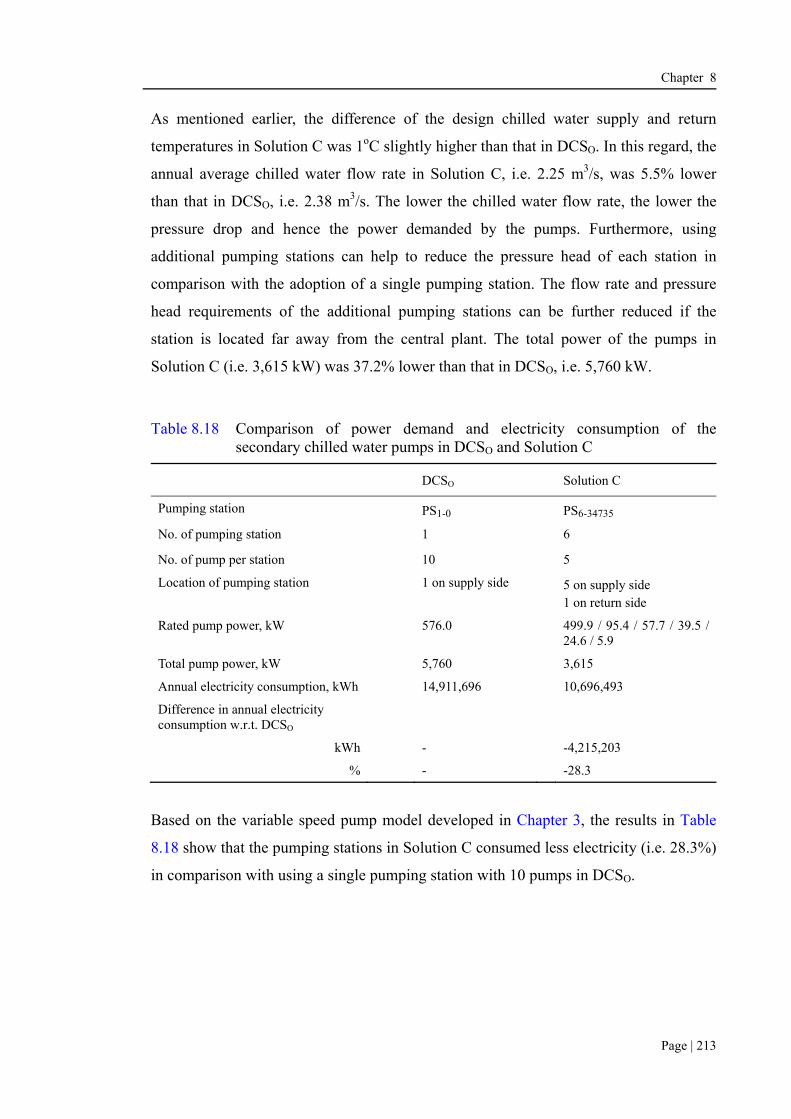
Chapter 8
Page | 213
As mentioned earlier, the difference of the design chilled water supply and return
temperatures in Solution C was 1oC slightly higher than that in DCSO. In this regard, the
annual average chilled water flow rate in Solution C, i.e. 2.25 m3/s, was 5.5% lower
than that in DCSO, i.e. 2.38 m3/s. The lower the chilled water flow rate, the lower the
pressure drop and hence the power demanded by the pumps. Furthermore, using
additional pumping stations can help to reduce the pressure head of each station in
comparison with the adoption of a single pumping station. The flow rate and pressure
head requirements of the additional pumping stations can be further reduced if the
station is located far away from the central plant. The total power of the pumps in
Solution C (i.e. 3,615 kW) was 37.2% lower than that in DCSO, i.e. 5,760 kW.
Table 8.18 Comparison of power demand and electricity consumption of the secondary chilled water pumps in DCSO and Solution C
DCSO Solution C
Pumping station PS1-0 PS6-34735
No. of pumping station 1 6
No. of pump per station 10 5
Location of pumping station 1 on supply side 5 on supply side 1 on return side
Rated pump power, kW 576.0 499.9 / 95.4 / 57.7 / 39.5 / 24.6 / 5.9
Total pump power, kW 5,760 3,615
Annual electricity consumption, kWh 14,911,696 10,696,493
Difference in annual electricity consumption w.r.t. DCSO
kWh - -4,215,203
% - -28.3
Based on the variable speed pump model developed in Chapter 3, the results in Table
8.18 show that the pumping stations in Solution C consumed less electricity (i.e. 28.3%)
in comparison with using a single pumping station with 10 pumps in DCSO.

Chapter 8
Page | 214
8.6 Environmental Benefits of Solution C
Based on the predicted annual electricity consumption in Table 8.15, the respective
annual and life-cycle (for a life span of 60 years) equivalent CO2 emissions incurred by
generation of electricity for DCSO and Solution C were estimated, as shown in Table
8.19. The CO2 emissions were assumed to be 197 tonnes per TJ of electricity consumed
(Yik et al., 2012). Results indicate that by adopting Solution C in lieu of base DCSO, the
greenhouse gas emissions over a life span of 60 years could be reduced by an equivalent
amount of 721,941 tonnes (i.e. 14.7%).
If the emissions reduction (Table 8.19) is to be credited to the DCS operator for the
purpose of a carbon trading scheme, the saving over a 60-year useful life cycle can
represent a net present value of HK$7 million (assessed against the base case). This
value was based on the carbon value of €4 (~HK$30) per tonne of carbon dioxide
quoted by the World Bank (2013).
Table 8.19 Annual and life-cycle greenhouse gas emissions from DCSO and Solution C
DCSO Solution C Difference [Solution C minus DCSO]
tonne %
Annual CO2 (eqv.) emissions, tonne 82,909 70,839 -12,070 -14.6
Life-cycle (60 yrs) CO2 (eqv.) emissions, tonne
4,974,542 4,250,337 -724,204 -14.6
8.7 Summary
The effectiveness of each of the three energy efficiency enhancement measures in
mitigating the impacts of a degrading temperature difference on the energy performance
of the base case DCSO was discussed in the preceding chapters.
This chapter is to study the synergy effect of integrating different combinations of these
three measures. A simple heuristic optimization-simulation algorithm was developed to
reduce the 1,447,680 options into 434,268 possible solutions for an evaluation of their

Chapter 8
Page | 215
energy, financial and environmental performance. The ultimate goal was to achieve a
cost-optimal solution, emerging as having the lowest LCC and the best energy and
environmental performance.
Results of energy simulation indicate that among the 434,268 possible solutions, matrix
S(CE,T7,PS6-35464) could lead to the greatest reduction in the electricity consumption of
DCSO. This energy-optimal design solution is referred to as Solution E.
On the other hand, based on the simulated energy consumption and cost data collected
about the major equipment in the chiller plant and pumping station, an LCC model was
developed to estimate the life-cycle cost-effectiveness of each possible solution. A
cost-optimal design named as Solution C, i.e. matrix S(CD,T5,PS6-34735), was
successfully identified.
This cost-optimal design consisted of 15 equally-sized variable speed chillers and six
pumping stations located at both the chilled water supply and return sides, and was
equipped with five pumps in each station. The chilled water supply and return
temperatures were set at 5 oC and 13oC, respectively.
As compared to Solution E, the electricity consumption of Solution C was about 1%
higher. This difference, however, is insignificant because it was mainly due to the
trade-off in electricity consumption associated with the chillers and the secondary
chilled water pumps. Furthermore, the 14.6% life-cycle energy cost saving that Solution
C could achieve is more than enough to offset the extra costs incurred by adopting the
energy efficiency enhancement measures.
Results of the LCC analysis show that Solution C was the most financially favourable.
After comparing the overall LCC of the base design, DCSO and Solution C, it was found
that the latter could generate an LCC saving of 7.5%, representing a reduction of
HK$322 million in present value.
In addition, the analysis illustrates that the cost-optimal solution could offer significant
protection to the environment by reducing the DCS’ carbon footprint by 14.6% in

Chapter 8
Page | 216
comparison with the base case. This should be considered whenever possible in any
LCC analysis in order to achieve a sustainable decision.
These findings are significant, as they can offer insights to the DCS designers and
owners about the energy and financial trade-offs associated with the design of a large
scale DCS. If an owner focuses only on the initial capital investment, the long-term
energy costs and the associated environmental impacts may be overlooked.

Chapter 9
Page | 217
Chapter 9
Conclusion and Suggestions for Future Research
9.1 Summary of Work Done and Key Findings
To promote energy efficiency and conservation, the Hong Kong government is planning
to set up DCS in some new development areas, which are the Kai Tak Development, the
West Kowloon Cultural District and the North East New Territories Development. The
DCS will supply chilled water to buildings in these new areas for centralized
air-conditioning. In 2010, the plan to build Hong Kong’s first DCS that uses direct
seawater-cooling for the Kai Tak Development area was confirmed. The project is
divided into three phases. About 10% of the total installed capacity was completed in
2013 and the other two stages are expected to be finished in 2017 and 2021 respectively.
The estimated maximum cooling demand would amount to 80,000 RT (about 280 MW)
when all buildings served by the DCS are occupied. VPF chilled water systems and
constant speed chillers were designed for this DCS.
As mentioned in Chapter 1, low delta-T in the distribution loop of chilled water systems
has been widely reported by many researchers over the last 25 years. There is no
exception for the chilled water system in DCS. The resulting problem is the
corresponding increase in the chilled water flow rate. Particularly at part load, the flow
rate and cooling load do not correspond to each other, and hence additional chillers are

Chapter 9
Page | 218
required to be on to maintain the flow requirements even though the maximum cooling
capacity of the chillers has not been fully reached. Both high pumping energy
consumption and reduced efficiency of the chillers operating at part load can lead to a
dramatic decrease in the overall energy efficiency of the DCS.
There are many causes of the low delta-T syndrome. Many methods have been proposed
in the areas of design, control and maintenance. Among them, the use of bypass check
valves and VPF pumping schemes have received great attention. However, there is no
universal conclusion of which solutions can absolutely help to mitigate the impacts of
low delta-T on the energy performance of DCS. In reality, some of the causes cannot be
avoided, such as the degradation of coil effectiveness.
A DCS should be designed to operate efficiently under low delta-T conditions. However,
well-documented and detailed simulation work or case study in designing a DCS to
accommodate the low delta-T has been lacking. In particular, regarding the VPF system
in Hong Kong’s first DCS under the Kai Tak Development project, there was a lack of
quantitative analysis for comparing the amount of energy saving after applying either
the P-S or VPF systems in the chilled water pumping system of a large scale DCS.
In this regard, all these have led to the need for a detailed investigation from a
comprehensive system design perspective to find out a design solution that can mitigate
the impacts of low delta-T on the energy performance of DCS. The findings can be
useful for DCS designers as the DCS can operate in an efficient manner with the
inevitable low delta-T. Furthermore, in view of the huge capital investment and lengthy
payback period of such a large scale infrastructural development project, this research
was geared towards finding a design solution that would be financially viable. It was
hoped that this solution could help the DCS owner identify a system design that could
strike a good balance between the initial costs and the long-term benefits.
9.1.1 Development of a Hypothetical District
As the first DCS in Hong Kong is still in an embryonic stage, it was more cost-effective
to adopt a model-based approach for this study instead of performing field research. As

Chapter 9
Page | 219
a result, a hypothetical district made up of office buildings, commercial complexes and
hotels was established. These buildings encompassed a combination of offices, retail
shops, restaurants and hotel guestrooms. The total design cooling capacity was about
200 MW, which was close to the scale of the biggest single DCS in Japan.
9.1.2 Design of a DCS
The comparative analysis results presented in Chapter 4 indicate that the VPF system is
unable to yield any significant saving in the electricity of a large scale DCS. The main
reason is that there were over 80% of the total operating pump hours in which the
pumps in the P-S and VPF systems were operated at a flow ratio greater than 80%.
Under such circumstances, the variable frequency drive decreases the efficiency of the
variable speed pump running at nearly full speed. It causes the variable speed pump to
consume more power than the CSP. As a result, the variable speed pumps and CSP in
the P-S system consume less electricity than the variable speed pumps in the VPF
system, so that the overall electricity consumption of the P-S system was 0.5% slightly
lower than that of the VPF system.
In this study, a P-S chilled water pumping scheme was designed for a baseline DCS -
DCSO. This DCS comprised a production loop, a distribution loop and building loops.
In the primary loop, a centralized chiller system configuration CO was designed with 10
constant speed chillers, which were equipped with dedicated primary chilled water
pumps and seawater pumps. Once-through direct seawater was used for heat rejection.
In the distribution loop, one pumping station, namely PS1-0, equipped with 10 variable
speed chilled water pumps was designed to distribute chilled water to each building in
the building loop. The design chilled water supply and return temperatures were 5oC
and 12oC respectively. Heat exchangers were used for the heat transfer of chilled water
in the distribution loop and each building in the building loops. DCSO was treated as a
base case for comparing the various options of the following energy efficiency
enhancement measures to improve the energy performance of the chiller plant and
pumping stations at low delta-T, as these two components are responsible for the major
portion of the total electricity consumption of the DCS.

Chapter 9
Page | 220
The first measure was to change the configuration of the chiller system. This was done
by altering the major influential design parameters such as the number, cooling capacity
and type (i.e. constant or variable speed) of the chillers. The second measure was related
to the pumping station. The variations included: application of multiple pumping
stations in different locations of the chilled water supply and return network, and using
different number of pumps in each pumping station. The third measure was to change
the design temperature of the chilled water supplied by the chiller plant and the design
temperature of the chilled water returning from the building. A sensitivity analysis of
different temperature regimes was performed accordingly.
9.1.3 Development of Mathematical Models for Energy and Cost Simulation
Almost all published mathematical models of the major air-conditioning equipment
such as chillers, cooling coils and heat exchangers have been developed for individual
buildings only. The operating conditions of this equipment in a building are different
from those in a DCS. Therefore, it was of a practical importance to develop a simple
and accurate model, which could represent the design of a DCS. Moreover,
mathematical models of a chilled water distribution network and variable speed pumps
had to be specially developed for this study.
In this regard, mathematical models of the major equipment in the chiller plant and
pumping station were tailor-built, as shown in Chapter 3. They could facilitate an
evaluation of the impacts of low delta-T and the assessment of the effectiveness of
various options of the three energy efficiency enhancement measures. Moreover, a life
cycle cost (LCC) model was developed in Chapter 8 to evaluate the financial viability of
various options of the measures over the 60-year operating life cycle of the DCS.
9.1.4 Impacts of Low Delta-T on the Energy Performance of DCSO
In DCSO, it was reported in Chapter 4 that the delta-T under normal conditions was in a
decreasing trend when the cooling load was increased to a full load. Eventually, it
decreased to a level close to the design value of 7oC. However, delta-T fell short of the
design level at low cooling loads and it gradually increased to a temperature close to the

Chapter 9
Page | 221
design value when the cooling load was increased to a full load. Furthermore, the
annual average chilled water flow rate required to distribute chilled water from the
chiller plant with a low delta-T was 77% higher than that under normal conditions.
Under such circumstances, additional chillers had to be staged on for 54% of the annual
operating hours to meet the excessive chilled water flow rate. There were 4,670 hours
(53% of the 8,760 hours in a year) in which one additional chiller was required to be
operated and 62 hours (1% of the 8,760 hours) in which two additional chillers were
required. It is because the increased chilled water flow rate has exceeded the design
value of chillers operating under normal conditions. This led to an increase in the annual
total electricity consumption of DCSO by 9.3% when operating at low delta-T, in
comparison with the normal condition. In this regard, it was worthwhile to study the
energy efficiency measures mentioned above to enhance the energy efficiency of DCSO.
9.1.5 Effects of Chiller System Configuration on the Energy Performance of
DCSO
Regarding chiller system configuration, it can be optimized by modifying the three
influential design parameters: number, cooling capacity and type of chillers. With
reference to the design of the baseline DCSO, five alternative configurations were
identified. The simulation results unveil that the chiller system configuration using more
or unequally-sized chillers would provide more opportunities in meeting the available
cooling capacity with the cooling load requirement. This can increase the average PLR
of the chillers and hence the overall COP of the chiller plant. However, the adoption of
additional or unequally-sized chillers could only lead to a limited saving in the annual
total electricity consumption of DCSO, as this saving was less than 2%, when compared
to using the baseline configuration with a low delta-T. The main reason is that chillers in
the DCS have a larger cooling capacity that ranges from 2,000 RT (7,034 kW) to 6,000
RT (21,102 kW). As a result, the adoption of more chillers with different cooling
capacities does not have a significant impact on the chillers with a better COP under
various part load conditions.

Chapter 9
Page | 222
On the other hand, it was found that variable speed chillers could significantly reduce
the total annual electricity consumption of DCSO, as they could lead to a reduction of up
to 9.9% in comparison with constant speed chillers. It is because the COP of variable
speed chillers at part load is better than that of constant speed chillers. The energy
efficiency of variable speed chillers is further improved when they are operated in a
seawater temperature below 25oC. This can bring an additional benefit of reducing the
electricity consumption of chillers. Therefore, although almost every chiller is affected
by the low delta-T syndrome, particularly at low cooling loads, high energy
performance of the variable speed chillers at part load can effectively lessen the
problems incurred by degrading delta-T.
Among the five alternative configurations, it was found that the combination of 15
unequally-sized variable speed chillers, i.e. 5 x 2,000 RT (7,034 kW), 5 x 4,000 RT
(14,068 kW) and 5 x 6,000 RT (21,102 kW), performed the best in terms of energy
saving. It could reduce 11.6% of the total annual electricity consumption of DCSO when
low delta-T occurred.
9.1.6 Effects of Pumping Station Configuration on the Energy Performance of
DCSO
In Chapter 6, two design initiatives related to pumping system configuration were
examined. The first was to adopt a multiple pumping station approach instead of using a
single pumping station, and the location of the stations could be anywhere at the chilled
water supply and return sides of the distribution loop. To further optimize the design,
the second initiative was to adopt an unequal number of pumps in each pumping station.
Mathematically, the search for an optimum pumping station design is a very
complicated issue, as it involves 1,024 possible combinations in the analysis. As a result,
a hydraulic gradient method was applied to conduct a quick assessment for identifying
only those combinations that were technically feasible. The number of combinations
was finally significantly reduced by 86% from 1,024 to 140. Failure cases often
occurred when the pumping station was located at the far end of the central DCS plant.
It is because the system’s pressure head requirement decreases as the distance from the

Chapter 9
Page | 223
central DCS plant increases. Meanwhile, the pumping station has to maintain a
minimum pressure drop across the heat exchangers in each building. Therefore, there
will be a situation in which the system pressure decreases to a value at a location where
the differential pressure between the chilled water supply and return cannot achieve the
minimum value with a booster pumping station.
The second initiative was to change the grouping of the pumping stations based on the
number of pumps in each station, i.e. whether there were 5, 10 or 15 pumps in each
pumping station. This would generate a total of 36,192 pumping station arrangements.
On the other hand, a dataset of rated power of 1,800 pumps was developed to determine
the rated pump power of thousands of variable speed pumps designed with various flow
rates and pump head requirements. To facilitate a simulation of the energy consumption
of thousands of pumping station arrangements, an optimization program with a
systematic approach was established to perform a more efficient calculation. Results of
simulation reveal that the adoption of six pumping stations (i.e. PS6-34564), which were
equipped with five pumps in each station, could lead to a 3% reduction in the annual
total electricity consumption of DCSO.
In DCSO where there was only one main pumping station for distributing chilled water
to all the buildings in the district, the chilled water flow rate and pressure head were
very high. Adding booster pumping stations can help to reduce pressure head of the
main pumping station. Moreover, the pressure head requirements of the booster
pumping stations can be further reduced if the pumping stations are located further
away from the central plant. This can help to reduce the pump size and power demand
of the main pumping station and the booster pumping station. The total power demand
and annual electricity consumption of the pumps in PS6-35464 were 25.6% and 23% less
than those of the pumps in DCSO respectively.

Chapter 9
Page | 224
9.1.7 Effects of Chilled Water Supply and Return Temperature on the Energy
Performance of DCSO
Changing the temperature of the supply and return chilled water will have significant
impacts on two determining factors of the DCS’ energy performance, i.e. the COP of
the chillers and the chilled water flow rate in the distribution network. In DCSO, the
supply chilled water temperature was set at 5oC and the chilled water return temperature
was 12oC. To simulate the effects of changing the design temperature, eight different
temperature regimes were identified. The energy performance of different components
in DCSO was then compared.
As reported in Chapter 7, the chiller’s COP increased as the chilled water supply
temperature was increased from 4oC to 6oC. In a situation where the PLR was greater
than 40%, the average percentage of increment in the COP ranged from 1.3% to 2% for
every oC of increase in the chilled water supply temperature. Regarding chilled water
flow rate, results show that the annual average chilled water flow rate was the highest
when the design temperature difference between the chilled water supply and return
temperature was at the lowest level, i.e. 5oC. Relatively lower chilled water flow rate
was required when the design temperature difference was at the highest level, i.e. 9oC.
The resulting COP of the chillers and the chilled water flow rate would in turn affect the
energy performance of the chiller plant and chilled water pumps in the DCS.
The simulation results also reveal that when the design chilled water supply and return
temperatures were 6oC and 11oC respectively, the annual total electricity consumption
of DCSO would be the lowest. Under this temperature regime, the chiller plant and the
pumping station exhibited different electricity consumption patterns. The energy
performance of the chiller plant was the best, due to a 4.6% of saving of electricity
when compared to other temperature regimes. It was because the design chilled water
supply temperature was on the high side of 6oC. The COP was thus relatively higher as
compared to other temperature regimes with a design supply temperature of 4oC or 5oC.
On the other hand, it was found that the secondary distribution pumps under this
temperature regime had the highest electricity consumption, i.e. 22.5% higher with

Chapter 9
Page | 225
reference to the base design. The reason is that the design temperature difference was at
the lowest level, i.e. 5oC. This can lead to a higher annual average chilled water flow
rate, and hence the design pump power and electricity consumption of the pumps.
Under such circumstances, the electricity saving of the chiller plant was nearly offset by
the increase in the electricity consumption of the secondary pumps. The overall
electricity consumption of DCSO could be reduced by about 1% when compared to the
baseline design.
9.1.8 A Cost-Optimal Integrated Design Solution
The simulation results presented in Chapters 5, 6 and 7 provide valuable information in
the design of a cost-optimal integrated solution for a DCS. By changing the design
parameters of the three energy enhancement measures, five combinations of chiller
plant configuration, and eight chiller water temperature regimes, 36,192 arrangements
of pumping station were derived. This could result in generating 1,447,680 possible
design solutions. A simple heuristic strategy was adopted to reduce this number by 70%
to 434,268. The energy, financial and environmental performances of these possible
solutions were then evaluated.
Based on the mathematical models developed in Chapters 3 and 6 for chiller plants and
pumping stations, an algorithm was formed in Chapter 8 for conducting simulations of
the electricity consumption of these possible solutions. The results show that the most
energy-optimal design (i.e. Solution E) could save 15.5% of the annual total electricity
consumption in comparison with that of DCSO. This solution encompassed 15 variable
speed chillers designed with three different cooling capacities. There were six pumping
stations at the chilled water supply side and each pumping station was equipped with
five pumps. The chilled water supply and return temperatures were 6oC and 12oC
respectively.
Based on the simulated energy consumption data and the cost information collected for
the major equipment in the chiller plant and pumping stations, an LCC analysis was
performed to estimate the LCC of each possible solution, including that of Solution E,
which had the best energy performance. It was found that instead of Solution E, another

Chapter 9
Page | 226
design - Solution C - was the most cost-optimal. This latter design had the lowest LCC,
which was 7.5% lower than that of the base case. The LCC saving in present value
would be over HK$332 million.
Solution C encompassed 15 equally-sized variable speed chillers. There were six
pumping stations at both the chilled water supply and return sides and each was
equipped with five pumps. The chilled water supply and return temperatures were 5 oC
and 13oC respectively. This design could lead to a 14.6% reduction in the electricity
consumption of DCSO. Although this percentage was about 1% lower than that
achieved by Solution E, the life-cycle energy cost saving from Solution C, which was
14.6%, was more than enough to offset the extra costs incurred by using additional
equipment and other devices associated with the energy efficiency enhancing measures.
Moreover, the LCC of this design was more financially favourable than that of Solution
E, even though the latter outmatched the former in terms of energy performance.
There is always a budgetary constraint for the DCS designer or owner to select an
optimum set of energy efficiency enhancement measures that can lead to the greatest
benefits. The value of the current research lies in the way that it helps to provide a
comprehensive review of the effectiveness of different energy efficiency measures. It
also helps to point to a direction in the search for an integrated design solution that can
mitigate the impacts of degrading delta-T on the energy performance of DCS. With all
this information, the DCS owner can be in a better position to weigh between the energy
benefits and the associated financial trade-offs. If a design decision is purely based on
initial capital investment, the long-term energy costs that a large scale infrastructure
development project can incur may be overlooked.
Moreover, the cost-optimal solution could offer a significant protection to the
environment by reducing the DCS’ carbon footprint by 14.6% in comparison with the
base case. This should be considered whenever possible in an LCC analysis in order to
achieve a sustainable future.

Chapter 9
Page | 227
9.2 Original Contributions of this Study
To the best of the author’s knowledge, this study is the first effort in conducting a
comprehensive assessment of the low delta-T issue in DCS from a system design’s
perspective. It has yielded the following key findings, which are original contributions
to knowledge in building services engineering.
9.2.1 One main contribution of this study is the development of a systematic
approach for conducting a thorough assessment of the effectiveness of
different possible design solutions so as to enhance the energy performance of
the chiller plant and the pumping station in DCS.
A cost-optimal design solution was identified. It was able to mitigate the
impacts of low delta-T on the DCS’ electricity consumption. The results
provide a guideline to the DCS designers with a considerable confidence
when designing the chiller plant and pumping station of other DCS with a
similar scale to accommodate the low delta-T issue in an energy efficient
manner.
9.2.2 Major efforts have been exerted in developing a vast number of mathematical
models for simulating the energy performance of all the major equipment in
the chilled water plant and pumping stations of the DCS. The models were
tailor-developed and could be applied for other DCS projects. Some new
improvements were made in the following models. These are not found in any
previous research literature.
i. Chiller Model
With the aid of a conventional bi-quadratic regression approach, the
regression variables for the constant and variable speed chillers were 16 and
15 respectively. Stepwise multiple regressions were applied to simplify the
mathematical models for these two types of chillers. This method could help
to select an appropriate set of regression variables from all the possible items

Chapter 9
Page | 228
and significantly reduce the number of regression variables to 6 and 5 for
constant and variable speed chillers respectively, and maintain a higher value
of determination of coefficient. This could help to simplify the structure of
the chiller models with a certain physical significance of variables that could
enable the model to make an accurate simulation of the chiller’s performance.
Most of the chiller models developed in other research studies are constructed
for applications in buildings rather than DCS. These models are always based
on a chilled water supply temperature of about 7oC. The chiller models
developed in this study were based on the part load performance data of
chillers with a design chilled water supply temperature as low as 4oC. This
chiller model can be widely used for other DCS research.
ii. Cooling Coil Model
There are tens of thousands of cooling coils of air supply equipment, i.e.
AHU, PAU and FAU in the buildings within a district. It was not practical to
study each of them. It is also not accurate to use a single cooling coil model
developed by other researchers to simulate the chilled water flow rate and
temperature of different types of buildings in a district. In this study, based on
the hourly cooling load and chilled water flow rate predicted by BECON, the
data was normalized and plotted to present the cooling coil characteristics of
the four model buildings A, B, C and D. These buildings were an office, a
low and a high rise commercial complex, and a hotel respectively.
Polynomial regression curves were plotted to fit for the normalized data, and
model the cooling coil output and the chilled water flow rate of each building
under normal conditions.
iii. Hydraulic Chilled Water Distribution Model
Hydraulic chilled water distribution models of the pipe network topology of
the DCS were built to simulate the dynamic and non-linear characteristic

Chapter 9
Page | 229
between the hourly chilled water flow rate and the corresponding pressure
drop along the distribution network.
9.2.3 There are over thousands of possible combinations of the number and
location of the pumping stations in the distribution loop. The hydraulic
gradient evaluation method was found to be an effective tool for designers to
make a quick assessment of the technical feasibility of different combinations
of pumping station design and identify the combinations that can meet the
required minimum pressure across the chilled water supply and return
pipework.
9.2.4 To facilitate a simulation of the power demand of ten thousand variable speed
pumps under different pumping station combinations, a comprehensive
dataset of the rated power of pumps with different sizes was obtained from
the manufacturers for developing a simple pump power model. This model
can help to provide an effective tool to designers in determining the power of
pumps with different sizes.
9.2.5 To help the DCS owners and designers strike an optimum balance between
the first costs and the energy benefits, an LCC model was developed to
evaluate the financial performance of different DCS design solutions. This
allows a more realistic determination of a cost- and energy-optimal design.
This also provides them with a reasonable support in the decision-making
process.
9.2.6 It has been proved in this study that variable speed chillers and multiple
pumping stations play a vital role in mitigating the impacts of the low-delta T
issue on the energy performance of DCS. The evaluation gives some useful
guidelines for designers in reviewing the application of VPF systems and
constant speed chillers for the DCS in the Kai Tak Development.
In the present study, a step-by-step and systematic approach was developed for
evaluating and integrating different energy efficiency measures for identifying a

Chapter 9
Page | 230
cost-optimal design solution that can mitigate the impact of low delta-T on the energy
performance of DCS. This approach and the energy efficiency measures provide useful
guidelines for DCS designers facing the inevitable low delta-T issue. Moreover, the
models developed particularly for chillers and building cooling coils provide a useful
basis for researchers in their future investigation. The chiller models is based on the part
load performance data of chillers with a design chilled water supply temperature as low
as 4oC. Moreover, the cooling coil model can well present the cooling coil
characteristics of buildings comprising office, commercial complex and hotel. Moreover,
the hydraulic gradient evaluation method was found to be an effective tool for designers
to make a quick assessment of the technical feasibility of different combinations of
pumping station design and identify the combinations that can meet the required
minimum pressure across the chilled water supply and return pipework.
9.3 Limitations and Recommendations for Further Research
Although the objectives of this research have been reached and some original
recommendations were made regarding the design of a DCS, this research has some
limitations. These limitations, however, may be seen as potential areas for future
research. It would be desirable and valuable to make further efforts in the following
aspects related to the findings presented in this thesis.
Firstly, effort has been made in this study to model the cooling coil characteristics at
low delta-T. However, most buildings did not have a comprehensive record of the
chilled water temperature and flow rate. It was therefore difficult to collect sufficient
information of the sample buildings operating under low delta-T conditions. Therefore,
an extensive field work is desirable for finding out the operational characteristics of the
cooling coils at low delta-T in different types of buildings. This can help to further
develop more accurate mathematical models for the cooling coils suffering from the low
delta-T problem.
Secondly, in the present study, a hypothetical district was developed based on the
operational characteristics of the air-conditioning systems of existing buildings. Upon
completion of the first phase of the DCS in the Kai Tak Development, even though the

Chapter 9
Page | 231
scale is not large, it is still worthy to conduct a more extensive field test concerning the
operational characteristics of the DCS so that a more comprehensive database can be
obtained to facilitate the evaluation of the energy performance of chiller plants and
pumping stations.
Last but not the least, a new type of water-cooled “oil-free” chillers has recently
emerged in the market. The use of magnetic bearings for supporting the shaft that
directly couples the motor with the compressor impeller and for fixing the axial position
of the shaft offers an advantage that the shaft will be suspended in air by magnetic flux
and so it makes no contact with any other parts in the chiller. As a result, the motor can
run at a very high speed (e.g. up to 30,000 rpm). This eliminates the need for lubricant
as well as a gear chain to step up the rotational speed of the motor to that of the impeller,
and can also minimize the associated energy loss. The electricity consumption of these
chillers at part load is relatively lower in comparison with the conventional
water-cooled chillers. However, these chillers are relatively new and expensive, and
their cooling capacity is limited to a maximum of 800 RT (2,814 kW). Extensive use of
these chillers is, therefore, considered premature. Nevertheless, it would be worthwhile
to investigate the potential of adopting these chillers in a DCS in the coming future and
explore their effectiveness in accommodating the low delta-T issue, typically at low
load.

Page | 232
BIBLIOGRAPHY
Alexander D.K., 1996, HTB2 - A model for the thermal environment of building in operation (Release 2.0a), User Manual, Welsh School of Architecture R&D, University of Wales, Cardiff, UK.
American Society of Heating, Refrigeration, and Air-conditioning Engineers (ASHRAE), 2001, ASHRAE Standard 62-2001: Ventilation for Acceptable Indoor Air Quality, Atlanta, GA.
American Society of Heating, Refrigeration, and Air-conditioning Engineers (ASHRAE), 2009, ASHRAE Handbook: Fundamentals, ASHRAE, Atlanta, GA.
American Society of Heating, Refrigeration, and Air-conditioning Engineers (ASHRAE), 2011, ASHRAE Handbook: Applications, ASHRAE, Atlanta, GA.
Anagnostopoulos J.S. and Papantonis D.E., 2007, Pumping station design for a pumped-storage wind-hydro power plant, Energy Conversion And Management, 48(11): 3009-3017.
Arup, 2014, The North East New Territories New Development Areas Planning and Engineering Study – Stage 3 Public Engagement Digest, Civil Engineering and Development Department, and Planning Department.
Avery G., 1998, Controlling chillers in variable flow systems, Heating/Piping/Air Conditioning Engineering, 73(4):41-50.
Bahnfleth W.P. and Peyer E.B., 2004, Variable Primary Flow Chilled Water Systems: Potential Benefits and Application Issues, Final Report to Air-Conditioning and Refrigeration Technology Institute.
Bahnfleth W.P. and Peyer E.B., 2006, Energy use and economic comparison of chilled-water pumping system alternatives, ASHRAE, 112:198-208.
Bhatia A., 2013, HVAC chilled water distribution schemes, Continuing Education and Development Engineering, retrieved on 15 Nov 2013, from http://www.cedengineering.com
Brandemuehl M.J., 1993, A Toolkit for Secondary HVAC System Energy Calculations, ASHRAE, Atlanta.
Brasz J.J. and Tetu L., 2008, Variable speed centrifugal chiller control for variable primary flow applications, International Refrigeration and Air Conditioning Conference at Purdue, July:1-12.

Page | 233
Bullet J.D., 2007, Variable flow chiller plant design, presented in Technical Session no. 6 of ASHRAE Region XI CRC, Tuesday 15th May 2007.
Cai H.W., 2009, Research on the Real Chilled Water System in Large-Scale Commercial Buildings, Master’s thesis, Tsinghua University.
Cai H.W., Chan C., Jiang Y., Wei Q.P. and Jean Q., 2012, Concise graphic-analytic method for chilled water system characteristics analysis, Proceedings of the 3rd Greater Pearl River Delta Conference on Building Operation and Maintenance - Green Building & Green Operation and Maintenance, China Science Literature Publishing House, 106-114.
Campbell M.J., Statistics at square two: understanding modern statistical applications in medicine. London, GBR: BMJ Publishing Group; 2001.
Cevik A., Gogus M.T., Guzelbey, I.H. and Filiz H., 2010, A new formulation for longitudinally stiffened webs subjected to patch loading using stepwise regression method, Advances in Engineering Software, 41:611-618.
Chan A.L.S., Hanby V.I. and Chow T.T., 2007, Optimization of distribution piping network in district cooling system using genetic algorithm with local search, Energy Conversion and Management, 48(10):2622-2629.
Chan C.W.H., 2006, Optimizing chiller plant control logic, ASHRAE Journal, 48(7):39-42.
Chan K.T. and Yu F.W., 2004, How chillers react to building loads, ASHRAE Journal, August:52-57.
Chang C., Wei Q.P. and Wang X., 2011, Assessing chilled water system retrofit through data-log-based simulation, Proceedings of Building Simulation 2011 - 12th Conference of International Building Performance Simulation Association, Sydney, 14-16 November.
Chang Y.H., Lee C.Y., Chen C.R., Chan C.J., Chen W.H. and Chen W.H., 2009, Evolution strategy based optimal chiller loading for saving energy, Energy Conservation and Management, 50:132–139.
Chow T.T., Au, W.H., Yau, R., Cheng V., Chan, A.L.S. and Fong K.F., 2004a, Applying district-cooling technology in Hong Kong, Applied Energy, 79(3):275-289.
Chow T.T., Fong, K.F., Chan, A.L.S., Yau, R., Au, W.H. and Cheng V., 2004b, Energy modeling of district cooling system for new urban development, Energy and Building, 36(1):1153-1162.

Page | 234
Clark S., Mardiat E.D., Swinson S.K., 2011, A Texas-sized district energy system: The energy behind what’s next at the Texas Medical Center, District Energy, International District Energy Association, 3rd Quarter: 12-17.
Dalin P., 2012, Free cooling/natural cooling is crucial for a successful district cooling development, paper presented in 2012 Annual Conference - Teaming up for renewable heating and cooling, Euroheat and Power.
Dalkia, 2009, Creating energy progress, paper presented at 100th Annual Conference, International District Energy Association.
Delbes J., 1999, District Cooling Handbook, European Marketing Group District Heating and Cooling.
Dielman T.E., 2005, Applied Regression Analysis, Brooks/Cole Thomson Learning, USA.
Doty S., 2011, Energy saving measure interactions in chilled water system, Energy Engineering, 108(5): 7-36.
Douglas J.F., 1985, Fluid Mechanics, Pitman Publishing, London.
Durkin T.H., 2005, Evolving design of chiller plants, ASHRAE Journal, Feb: 28-34.
Eaton, 2011, Adjustable Frequency Drives, Eaton, USA.
Electrical and Mechanical Services Department (EMSD), 1999, Preliminary phase consultancy on wider use of water cooled air conditioning system in Hong Kong – Final report, Consultancy Report, Electrical and Mechanical Services Department, Hong Kong.
Electrical and Mechanical Services Department (EMSD), 2000, Pilot scheme for wider use of fresh water evaporative cooling towers for energy-efficient air conditioning systems, Electrical and Mechanical Services Department, Hong Kong.
Electrical and Mechanical Services Department (EMSD), 2002, Implementation of district cooling system at SEKD, Legislative Council Panel on Environmental Affairs, Hong Kong.
Electrical and Mechanical Services Department (EMSD), 2003a, Implementation study for a district cooling at South East Kowloon development – Executive Summary, Consultancy Report, Hong Kong.
Electrical and Mechanical Services Department (EMSD), 2003b, Territory-wide implementation study for water cooled air conditioning systems in Hong Kong – Executive Summary, Hong Kong.

Page | 235
Electrical and Mechanical Services Department (EMSD), 2003c, Territory-wide implementation study for water cooled air conditioning systems in Hong Kong – Final Report, Hong Kong.
Electrical and Mechanical Services Department (EMSD), 2004, Pilot scheme for wider use of fresh water in evaporative cooling towers for energy efficient air conditioning system – 2004 Achievement Summary, Hong Kong.
Electrical and Mechanical Services Department (EMSD), 2005, Implementation study for water-cooled air conditioning systems at Wan Chai and Causeway Bay – Investigation: Executive Summary, Hong Kong
Electrical and Mechanical Services Department (EMSD), 2012a, EMSD code of practice for energy efficiency of building services installation, Hong Kong.
Electrical and Mechanical Services Department (EMSD), 2012b, Hong Kong energy end-use data, Hong Kong.
Electrical and Mechanical Services Department (EMSD), 2012c, Technical guidelines for connection to district cooling system (Draft), Hong Kong.
Electrical and Mechanical Services Department (EMSD), 2013, District cooling system, retrieved on 15 Nov 2013, from http://www.energyland.emsd.gov.hk/en/building/district_cooling_sys/dcs.html
Energy Market Authority (EMA), 2002, Price regulation for district cooling services, consultation document, Energy Market Authority of Singapore, Singapore.
Energy Market Authority (EMA), 2009, District cooling services supply code, Energy Market Authority of Singapore, Singapore
Environment Bureau, 2013, PWP Item No. 45CG - District Cooling System at the Kai Tak Development, Legislative Council Panel on Environmental Affairs, Hong Kong.
Evans M., 2006, Possibilities with More District Cooling in Europe, Euroheat & Power, Belgium.
Field B.C. and Field M., 2009, Environmental Economics: An Introduction, McGraw-Hill International, New York.
Fiorino D.P., 1999, Achieving high chilled-water delta Ts, ASHRAE Journal, 41(11):24-30.

Page | 236
Friotherm A.G., 2013, High demand for district cooling and heating in Stockholm, Stockholm, Sweden, retrieved on 15 Nov 2013, from http://www.friotherm.com/webautor-data/41/nimrod_e009_uk.pdf
Fuller S.K. and Petersen S.T., 1996, Life-cycle costing manual for the federal energy management program, 1995th edition, Washington DC: U.S. Department Energy.
Gordon J.M., Ng K.C. and Chui H.T., 1995, Centrifugal chillers: Thermodynamic modelling and a diagnostic case study, International Journal of Refrigeration, 18(4):253-257.
Hartman T., 2001, Getting real about low delta T in variable-flow distribution systems, Heating/Piping/Air Conditioning Engineering, 73(4):17.
Helsinki Energy, 2006, Prospects for district cooling, retrieved from http://www.helsinginenergia.fi
Ho P.Y., 2003, Weathering the Storm: Hong Kong Observatory and Social Development, Hong Kong University Press, Hong Kong.
Hovde P.J. and Moser K., 2004, Performance Based Methods for Service Life Prediction, State of Art Reports, CIB.
Hydeman M., Sreedharan P., Webb N. and Blanc S., 2002, Development and testing of a reformulated regression-based electric chiller model, ASHRAE Transactions, 108(2):1118-27.
Hyman L.B. and Little D., 2004, Overcoming low delta T, negative delta P - at large university campus, ASHRAE Journal, 46(2):28-34.
International Energy Agency (IEA), 2002, Optimization of Cool Thermal Storage and Distribution, International Energy Agency, Novem, Netherlands.
Japan for Sustainability, 2009, A key to urban comfort and efficiency - Japan's district heating and cooling systems, Newsletter, June, No. 82.
Kirsner W., 1996, The demise of the primary-secondary pumping paradigm for chilled water plant design, Heating/Piping/Air Conditioning Engineering, 68(11):73-78.
Kirsner W., 1998, Rectifying the primary-secondary paradigm for chilled water plant design to deal with low ΔT central plant syndrome, Heating/Piping/Air Conditioning Engineering, 70(1):128-31.
Kuretich K.M., 2010, Large-campus district cooling, Heating/Piping/Air Conditioning Engineering, 82(5):26-33.

Page | 237
Lam K.K., 1997, Performance Evaluation of Chiller System, Master’s Thesis, Department of Building Services Engineering, Hong Kong Polytechnic University.
Landman W., 1996, Off-design chiller performance, Trane Engineers Newsletter, 25(5).
Lebrun J., 1999, A Toolkit for Primary HVAC System Energy Calculations, ASHRAE, Atlanta.
Lee W.L. and Lee S.H., 2007, Developing a simplified model for evaluating chiller-system configurations, Applied Energy, 84:290-306.
Leung Y.K., Wu M.C., Yeung K.K. and Leung W.M. 2007, Temperature projections for Hong Kong based on IPCC fourth assessment report, Hong Kong Meteorological Society Bulletin, Volume 17, HKO Reprint No. 764.
Lo A.C.W., Yik F.W.H and Jones P., 2006, Techno-economic assessment and optimization of district cooling system in a mega-city, paper presented at the 2nd Mega Cities International Conference 2006, Guangzhou.
Lomas K.J., Eppel H., Martin C.J. and Bloomfield D.P., 1997, Empirical validation of building energy simulation programs, Energy and Buildings, 26:253-275.
Luther K., 2002, Chilled water system forensics, ASHRAE Transactions, 108(1):654-8.
Ma S.W.Y., Kueh C.S.W., Chiu G.W.L., Wild S.R. and Yip J.Y., 1998, Environmental management of coastal cooling water discharges in Hong Kong, Water Science and Technology, 38(8-9):267–274.
Ma Z.J. and Wang S.W., 2011, Enhancing the performance of large primary-secondary chilled water systems by using bypass check valve, Energy, 36:268-276.
Majid M. A.A., Gilani S.I. and Rangkuti C., 2008, Gas District Cooling in Malaysia: Pioneering a new industry, District Energy, International District Energy Association, 3rd Quarter: 14-18.
Marchi A., Simpson A.R., and Ertugrul N., 2012, Assessing variable speed pump efficiency in water distribution systems, Drinking Water Engineering and Science, 5: 15-21.
Masters G.M. and Ela W.P., 1998, Introduction to Environmental Engineering and Science, Prentice-Hall, USA.
McQuay, 2002, Chiller Plant Design - Application Guide, McQuay International, Minesota, USA.

Page | 238
McQuay International, 2001, Parallel-Chiller Plants, McQuay International, Minesota, USA.
Moe E.M., 2005a, Building performance with district cooling, ASHRAE Journal, July: 46-53.
Moe E.M., 2005b, Applying pressure independent control to achieve high delta-T, International District Energy Association (IDEA) Annual Conference, Nashville, TN.
Montgomery D.C. and Runger G.C., 2010, Applied Statistics and Probability for Engineers, John Wiley & Sons, New York.
NCSS, 2013, NCSS manual, NCSS Statistical Software, USA, Chapter 311:1-9.
Nuon, 2013, District cooling in Amsterdam’s Zuidas, retrieved on 15 Nov 2013, from http://www.web-logix.nl/CreativeEnergy/content/visits/folder_Zuidas.pdf
Onyiah L.C., 2009, Design and Analysis of Experiments, CRC Press, USA.
PACO, 2014, PACO Pump Catalogue.
Qureshi T. Q. and Tassou S.A., 1996, Variable-speed control in refrigeration systems, Applied Thermal Engineering, 16(2):103-113.
Rabehl R.J., Mitchell J.W. and Beckman W.A., 1999, Parameter estimation and the use of catalog data in modeling heat exchangers and coils, HVAC&R Research, 5(1):3-17.
Rishel J. B., 2000, 40 years of fiddling with pumps, ASHRAE Journal, 42(3):43-49.
Rishel J. B., 2001, Wire-to-Water Efficiency of Pumping System, ASHRAE Journal, 43(4):40-46.
Rishel J., Durkin, T and Kincaid B., 2006, HVAC Pump Handbook, Second Edition, McGraw Hill Company, Inc., USA
Sat P.S.K. and Yik F.W.H., 2003, Comparison of predictions of the building energy simulation programs HTB2 and BECON with metered building energy data, HKIE Transactions, 10(3):34-47.
Schwedler M. and Bradley B., 2000, An idea for chilled water plants whose time has come… Variable-Primary-Flow Systems, Heating/Piping/Air Conditioning Engineering, 72(4):41-44.

Page | 239
Severini S.C., 2004, Making them work: Primary-secondary chilled water systems, ASHRAE Journal, 46(7):27-33.
Shiu K. S., 2000, Implementation of gas district cooling and cogeneration in Malaysia, International Gas Engineering and Management, 40:93-100.
Siemens, 2006, Pressure-independent control valves vs. high performance control valves, Technology Report (Document No. 149-990), Siemens Industry Inc.
Ssegane H., Tollner E.W., Mohamoud Y.M., Rasmussen T.C., Dowd J.F., 2012, Advances in variable selection methods I: Causal selection methods versus stepwise regression and principal component analysis on data of known and unknown functional relationships, Journal of Hydrology, 438–439:16-25.
Skagestad B. and Mildenstein P., 1999, District Heating and Cooling Connection Handbook, The International Energy Agency, Novem, Netherlands.
Stoecker W.F., 1975, Procedures for Simulating the Performance of Components and Systems for Energy Calculations, ASHRAE, Atlanta, GA.
Tam A., 2014, Air-conditioning the target of district-wide scheme to reduce energy use, Hong Kong Engineer, 42:8-13.
Taylor Engineering, 2009, Chilled Water Plant Design Guide, Taylor Engineering, Alameda.
Taylor S.T., 2002a, Degrading chilled water plant delta-T: Causes and mitigation, ASHRAE Transaction, 108(1):641-53.
Taylor S.T., 2002b, Primary-only vs primary-secondary variable flow systems, ASHRAE Journal, 44(2):25-29.
Taylor S.T., 2003, Control of variable primary flow chilled water systems, presented at ASHRAE Annual Meeting.
Taylor S.T., 2011, Optimizing design and control of chilled water plants – Part 3: Pipe sizing and optimizing delta T, ASHRAE Journal, 53(12):22-34.
Taylor S.T., 2012, Optimizing design and control of chilled water plants – Part 5: Optimized control sequences, ASHRAE Journal, 54(6):56-74.
Tey P.K., 2010, District cooling as an energy and economically efficient urban utility – Its implementation at Marina Bay business district in Singapore, presented in an evening talk organised by IES Power & Energy Interest Group, on 30 June 2010.

Page | 240
Trading Economics, 2013, Hong Kong Inflation Rate, retrieved on 15 Nov 2013, from http://www.tradingeconomics.com/hong-kong/inflation-cpi
Trane, 1989, Chiller plant system performance, Engineers Newsletter, 18(2).
Trane Hong Kong, 2013, Variable Primary Water Flow Systems.
Underwood C.P. and Yik F.W.H, 2004, Modelling Methods for Energy in Buildings, Blackwell Publishing, USA.
Wan K.S.Y., 1998, Comparison of Predicted Cooling Load and Plant Performance with Measured Data from an Existing Building, MEng Dissertation, Department of Building Services Engineering, Hong Kong Polytechnic University.
Wang L.P., Haves P and Buhl F., 2012a, An improved simple chilled water cooling coil model, paper presented at the SimBuild 2012 IBPSA Conference, Environmental energy and Technologies Division, Ernest Orlando Lawrence Berkeley National Laboratory, Berkeley, CA.
Wang L., Watt J. and Zhao J., 2012b, Model based building chilled water loop delta-T fault diagnosis, paper presented at the Twelfth International Conference for Enhanced Building Operation, Manchester, UK, October 23-26.
Wang S.W., Ma Z.J. and Gao D.C., 2010, Performance enhancement of a complex chilled water system using a check valve: Experimental validation, Applied Thermal Engineering, 30(17-18):2827-32.
Wang Y.W., Cai W.J., Soh Y.C., Li S.J., Lu L. and Xie L.H., 2004, A simplified modeling of cooling coils for control and optimization of HVAC systems, Energy Conversion and Management, 45:2915-2930.
Wei Z. and Zmeureanu R., 2009, Energy analysis of variable air volume systems for an office building, Energy Conversion and Management, 50(2):387-392.
Wikipedia, 2013, District cooling, retrieved on 15 November 2013, from http://en.wikipedia.org/wiki/District_cooling
Wong W.L. and Ngan K.H., 1993, Selection of an example weather year for Hong Kong, Energy & Buildings, 19:313- 316.
Wong F.Y.H. and Tang Y. T., 2010, Comparative life-cycle carbon footprint study of a proposed district cooling system and conventional HVAC Systems for Hong Kong’s new urban developments, paper presented in the 16th Annual International Sustainable Development Research Conference.

Page | 241
Wong K.W., 1997, Design of Chilled Water System for High Rise Buildings, MSc Dissertation, Department of Building Services Engineering, Hong Kong Polytechnic University.
World Bank, 2013, Mapping Carbon Pricing Initiatives – Development and Prospects 2013, World Bank Institute, Washington DC.
Wu Y. and Rosen M.A., 1999, Assessing and optimizing the economic and environmental impacts of cogeneration/district energy system using an energy equilibrium model, Applied Energy, 62:141-154.
Wulfinghoff D.R, 2004, Energy Efficiency Manual, Energy Institute Press, Wheaton, Maryland, United States.
Yang, Jinming and Lin Yi, 2012, Control algorithms and control strategies for primary flow chilled water systems, The 2nd International Conference on Computer Application and System Modelling, pp. 634-637.
Yang K.H. and Ting M.M., 2000, An innovative analysis and experimental investigation on energy savings of a VAV system in hot and humid climates, Building and Environment, 35(1):27-31.
Yates A., 2001, Quantifying the business benefits of sustainable buildings – Summary of existing research findings (extracts), draft for discussion, February 16, 2001, extracted from http://www.usgbc.org
Yik F.W.H., 1996, BECON – A Building Energy Consumption Estimation Program, User Manual, Department of Building Services Engineering, The Hong Kong Polytechnic University, Hong Kong.
Yik F.W.H., 1999, Selection of control valves for air conditioning systems, the Hong Kong Institution of Engineers Transactions, 6(2):11-18.
Yik F.W.H., 2012, Building Energy Evaluation Program - User Manual for BEEP (v.1.0), Department of Building Services Engineering, Hong Kong Polytechnic University, Hong Kong.
Yik F.W.H., Burnett J. and Prescott I., 2001a, A study on the energy performance of three schemes for widening application of water-cooled air-conditioning systems in Hong Kong, Energy and Buildings, 33:167-182.
Yik F.W.H., Burnett J. and Prescott I., 2001b, Predicting air conditioning energy consumption of a group of building using different heat rejection methods, Energy and Buildings, 33:151-16.

Page | 242
Yik F.W.H., Burnett J., Lee W. L. and Prescott I., 1999, Chiller plant sizing by cooling load simulation as a means to avoid oversized plant, HKIE Transactions, 6(2):19-25.
Yik F.W.H., Lai J., Leung P.H.M. and Yuen P.L., 2012, A case study on the application of air- and water-cooled oil-free chillers to hospitals in Hong Kong, Building Services Engineering Research & Technology, 33(3):263-279.
Yik F.W.H. and Lam V.K.C., 1998, Chiller models for plant design studies, Building Services Engineering Research and Technology, 19(4):233-241.
Yu F.W., 2009, Environmental performance and economic analysis of all-variable speed chiller systems with load-based speed control, Applied Thermal Engineering, 29:1721-1729.
Yu P.C.H., 2001, A study of Energy Use for Ventilation and Air-conditioning System in Hong Kong, PhD Thesis, Department of Building Services Engineering, Hong Kong Polytechnic University.
Zhan X., Liang, X., Xu G. and Zhou L., 2013, Influence of plant root morphology and tissue composition on phenanthrene uptake: Stepwise multiple linear regression analysis, Environmental Pollution, 179:294-300.
Zhang Z.Q., Li, H. and Liu, J.J., 2012, Simulations of chilled water cooling coil delta-T characteristic, ASHRAE Transactions, 118(2):349-356.