Optimizing Solvent Extraction of PCBs

from Soil

by

Maureen O’Connell

A thesis

presented to the University of Waterloo

in fulfillment of the

thesis requirement for the degree of

Master of Applied Science

in

Civil Engineering

Waterloo, Ontario, Canada, 2009

© Maureen O’Connell 2009

ii

AUTHOR'S DECLARATION

I hereby declare that I am the sole author of this thesis. This is a true copy of the thesis, including any

required final revisions, as accepted by my examiners.

I understand that my thesis may be made electronically available to the public.

iii

Abstract

Polychlorinated biphenyls (PCBs) are carcinogenic persistent contaminants. Although their

manufacturing in North America ceased in the late 1970s, their high heat resistance made their use

widespread over their production lifetime. As a result, PCB contamination has occurred globally and

in particular has plague brownfield redevelopment in urban environments. The remediation of PCB

contaminated soil or sediments has historically been dealt with through the expensive and

unsustainable practice of excavation followed by off-site disposal or incineration. One potential

technology that has shown some success with on-site remediation of PCB contamination is solvent

extraction. Solvent extraction is technically simple; it involves excavating the contaminated soil,

placing it in a vessel and adding solvent. The PCBs are extracted by the solvent and the treated soil is

returned for use on site. Although successful at removing a large quantity of PCBs from some soils,

this technology can be improved upon by extracting additional PCB mass and making the extraction

more efficient and suitable for colder climates.

This thesis aimed to identify the factors controlling PCB extraction with solvents in order to optimize

PCB extraction as it is applied on different soil types and in various climates. The research

investigated the impact of elevated moisture contents (≤ 20% by weight) on solvent extraction

efficiency, the effects of low temperatures (<5ºC) on solvent extraction, and developed a kinetic

model to represent PCB solvent extraction. As past research has shown, weathered PCB in soil is

more difficult to remove. Contaminated field samples from Southern Ontario, Canada were used for

this work, rather than synthetically prepared samples.

The impact of elevated moisture contents and low temperature on extraction efficiency was

determined through a series of screening experiments using polar and non-polar solvents at both 20ºC

and 4ºC. It was hypothesized that improved extractions may be possible with combinations of polar

and non-polar solvents. Based on the results of these screening experiments, a factorial experiment

was designed using solvent combinations to further assess the role of moisture contents and low

temperatures. The role of PCB mass distribution among grain sizes was also evaluated to see if

optimization based on grain size separation is possible. Finally, experiments were performed to

generate data suitable for the development of a kinetic model that incorporates key factors affecting

solvent extraction.

iv

Four suitable solvents for solvent extraction in Ontario were identified through a literature review and

these were used for this work: isopropyl alcohol (polar), ethanol (polar), triethylamine (non-polar)

and isooctane (non-polar). Triethylamine outperformed isooctane and performed best on its own

rather than in combination with polar solvents. An interaction between soil moisture content and

choice of polar solvent (isopropyl alcohol versus ethanol) was established: a given polar solvent

achieves optimal PCB extraction at a specific moisture content range. Temperature was also

identified as significantly influencing PCB extraction. Although it was determined that PCBs were

distributed unevenly amongst grain sizes, a simple relationship between grain size and fractional

organic carbon or organic content was not found.

A simple two-compartment kinetic model was developed which is suitable for predicting the PCB

concentrations extracted up to 24 hours. The model incorporates both temperature and soil to solvent

ratio in order to estimate PCB concentration extracted.

v

Acknowledgements

I would like to thank Dr. Neil Thomson for providing me with this learning opportunity, for his

determination to see this project through despite the many obstacles encountered, and for demanding I

continue to improve my data interpretation and writing. Thank you to the Ontario Centers of

Excellence for providing project funding and to Dr. Eric Reiner and Tony Chen from the Ontario

Ministry of the Environment for taking the time to show me how they do PCB analysis and answering

countless questions.

I would also like to thank the numerous co-op students who have helped me in the lab: Christina

Bright, Harry Oh, David Thompson, Tanyakarn Treeratanaphitak, Daniel Princz and finally Victoria

Chennette. I enjoyed working with all of you! I would like to thank Mark Sobon and Bruce Stickney

for providing invaluable lab support.

Thank you to my family and friends for their support throughout this degree, especially Bill

O’Connell and Jessica Pickel for proof reading draft thesis chapters. Finally, I would like to thank

my husband Jonathan Musser for his patience, encouragement, friendship and love.

vi

Dedication

I would like to dedicate my thesis to my late grandmother Betty O’Connell.

vii

Table of Contents  

List of Figures ........................................................................................................................................ x 

List of Tables ........................................................................................................................................ xii 

Chapter 1 Introduction ............................................................................................................................ 1 

1.1 Research Objectives ..................................................................................................................... 4 

1.2 Thesis Scope ................................................................................................................................. 4 

Chapter 2 Background and Literature Review ....................................................................................... 5 

2.1 Chemical Structure of PCBs ......................................................................................................... 5 

2.2 PCB Properties ............................................................................................................................. 5 

2.3 Current Remedial Strategies ......................................................................................................... 6 

2.3.1 In-Situ .................................................................................................................................... 6 

2.3.2 Ex-Situ ................................................................................................................................... 7 

2.4 Solvent Extraction Systems .......................................................................................................... 9 

2.4.1 CF-Systems ........................................................................................................................... 9 

2.4.2 B.E.S.T ................................................................................................................................ 10 

2.4.3 Carver-Greenfield Process ................................................................................................... 11 

2.4.4 Extraksol Process................................................................................................................. 12 

2.4.5 Terra-Kleen ......................................................................................................................... 13 

2.5 Factors Influencing Solvent Selection ........................................................................................ 13 

2.5.1 Solvent Toxicity .................................................................................................................. 13 

2.5.2 Solvent Polarity ................................................................................................................... 14 

2.5.3 Solvent Viscosity ................................................................................................................. 14 

2.5.4 Solvent Freezing Point ........................................................................................................ 15 

viii

2.5.5 Solvent Boiling Point .......................................................................................................... 15 

2.5.6 Solvent Cost ........................................................................................................................ 16 

2.5.7 Solvent Selection ................................................................................................................. 16 

2.6 Properties Controlling PCB Sorption and Desorption ................................................................ 17 

2.6.1 Soil Composition ................................................................................................................. 17 

2.6.2 Soil Grain Size ..................................................................................................................... 19 

2.6.3 PCB Composition ................................................................................................................ 19 

2.6.4 Temperature ......................................................................................................................... 20 

2.7 Modeling Sorption ...................................................................................................................... 22 

2.8 Modeling Desorption .................................................................................................................. 24 

Chapter 3 Methods & Materials ........................................................................................................... 34 

3.1 Experimental Design .................................................................................................................. 34 

3.1.1 Single Solvent Screening Experiments ................................................................................ 34 

3.1.2 Solvent Combination Experiments ...................................................................................... 35 

3.1.3 PCB Mass Distribution ........................................................................................................ 35 

3.1.4 Kinetic Experiments ............................................................................................................ 36 

3.2 PCB Sample Origin .................................................................................................................... 36 

3.3 PCB Analysis Procedures ........................................................................................................... 37 

3.3.1 Soil Extraction Methods ...................................................................................................... 37 

3.3.2 Analytical Soil Extraction ................................................................................................... 38 

3.3.3 Sample Clean-Up................................................................................................................. 38 

3.3.4 Gas Chromatograph Analysis .............................................................................................. 39 

3.3.5 Comparisons with Accredited Laboratories ........................................................................ 39 

3.4 QA/QC ........................................................................................................................................ 40 

ix

Chapter 4 Results and Discussion ........................................................................................................ 49 

4.1 Mass Balance Considerations ..................................................................................................... 49 

4.2 Moisture Content Effects on Solvent Extraction ........................................................................ 50 

4.2.1 Polar Solvents: At Room Temperature ................................................................................ 50 

4.2.2 Polar Solvents: At Lower Temperatures ............................................................................. 51 

4.2.3 Non-polar solvents: At Room Temperature ........................................................................ 52 

4.3 Solvent Combination Experiment .............................................................................................. 53 

4.3.1 ANOVA Results for 24 Factorial Experiment ..................................................................... 54 

4.4 PCB Mass Distribution ............................................................................................................... 54 

4.4.1 PCB Mass Distribution in Dixie0707 Soil .......................................................................... 54 

4.4.2 PCB Mass Distribution in Dixie0208 Soil .......................................................................... 55 

4.5 Effects of Moisture Content, Solvent Choice, Temperature and Grain Size on PCB Extraction

.......................................................................................................................................................... 56 

4.6 Kinetic Experiments ................................................................................................................... 57 

Chapter 5 Conclusions and Recommendations .................................................................................... 78 

5.1 Conclusions ................................................................................................................................ 78 

5.2 Recommendations ...................................................................................................................... 79 

Bibliography ......................................................................................................................................... 80 

Appendix A Ranking Potential Solvents .............................................................................................. 84 

x

List of Figures Figure 2.1. Solvent viscosity versus temperature (Lide, 1998) ............................................................ 32 

Figure 2.2. Solvent viscosity versus percent solvent mass (Lide, 1998) .............................................. 32 

Figure 2.3. Solvent freezing points versus percent solvent mass (Lide, 1998) .................................... 33 

Figure 2.4. PCB mass extracted with ethyl acetate over time (Valentin, 2000) ................................... 33 

Figure 3.1. (a) Images of ethanol and isooctane reactors following 24hr extraction, (b) Image of

reactors used to determine volume of solvent layers (isopropyl alcohol and isooctane at 20% moisture

content) ................................................................................................................................................. 47 

Figure 3.2. Grain Size Analysis of (a) Dixie0707 Soil and (b) Dixie0208 Soil ................................... 48 

Figure 4.1. (a) PCB concentration removed using isopropyl alcohol at 20ºC, (b) PCB concentration

remaining in soil having undergone experimental extraction with isopropyl alcohol at 20ºC, (c) PCB

concentration extracted using isopropyl alcohol at 20ºC - repeat, (d) PCB concentration extracted

using isopropyl alcohol at 4ºC, (e) PCB concentration remaining in soil having undergone

experimental extraction with isopropyl alcohol at 4ºC ......................................................................... 67 

Figure 4.2. PCB concentration removed using ethanol at 20ºC (a) with DCB recovery corrections and

(b) without DCB recovery corrections, PCB concentration in soil having undergone experimental

extraction with ethanol at 20ºC (c) with DCB recovery corrections and (d) without DCB recovery

corrections, (e) PCB concentration removed from dry soil using Ethanol at 4ºC, (f) PCB

concentration remaining in dry soil after extraction with ethanol at 4ºC ............................................. 68 

Figure 4.3. Percent mass extracted at 20ºC with (a) isopropyl alcohol and (b) ethanol ....................... 69 

Figure 4.4. Reactors following isopropyl alcohol extraction at (a) 20ºC, (b) 20ºC –repeat, (c) 4ºC, (d)

4ºC - 0% and 5% moisture content reactors only ................................................................................. 69 

Figure 4.5. Ethanol following extraction at (a) 20ºC –decanted ethanol, (b) 4ºC - reactors ................ 70 

Figure 4.6. Mean PCB mass removed at 4ºC using (a) isopropyl alcohol and (b) ethanol .................. 70 

Figure 4.7. PCB concentration extracted at 20ºC with (a) isooctane and (b) triethylamine, PCB

concentration remaining in soil after extraction at 20ºC with (c) isooctane and (d) triethylamine ...... 71 

Figure 4.8. Mean PCB mass removed at 20 ºC using (a) isooctane and (b) triethylamine ................... 71 

Figure 4.9. Reactors after experimental extraction at 20ºC with (a) isooctane and (b) triethylamine .. 72 

Figure 4.10. PCB concentration extracted with decanted solvent data at (a) 20ºC and (b) 4ºC. PCB

concentration remaining in soil following extractions at (c) 20ºC and (d) 4ºC. ................................... 73 

Figure 4.11. Percent PCB mass extracted using sum of soil and solvent data at (a) 20ºC and (b) 4ºC 74 

xi

Figure 4.12. PCB concentration distribution by grain size for (a) Dixie0707, (b) Dixie0208, (c)

Dixie0208 – without DCB recovery corrections, (d) Dixie0208 - repeat ............................................. 75 

Figure 4.13. Solvent following PCB extraction from grain size groupingswith ASE200 .................... 76 

Figure 4.14. PCB contaminated soil sorted by grain size (a) Dixie0208 and (b) Dixie0707 ............... 76 

Figure 4.15. (a) Percent organic content by weight for different grain sizes, (b) Percent fractional

organic carbon by weight for different grain sizes ............................................................................... 76 

Figure 4.16. PCB Extraction over time using a (a) 1g:1mL soil to solvent ratio at 20ºC, (b) 1g:0.75mL

soil to solvent ratio at 20ºC, and (c) 1g:1mL soil to solvent ratio at 4ºC ............................................. 77 

xii

List of Tables Table 2.1. Composition of PCB Isomer Groups from Erickson (Erickson, 1993) ............................... 27 

Table 2.2. Examples of PCB octonol-water partition coefficients (Hawker and Connell, 1988) ........ 27 

Table 2.3. Dielectric Constants (Lide, 1998) ........................................................................................ 28 

Table 2.4. Freezing and Boiling Points of Alcohols (Streitwieser et al., 1992) ................................... 29 

Table 2.5. Freezing and Boiling Points of Non-Alcohols .................................................................... 29 

Table 2.6. Pure Solvent and Azeotrope Boiling Points ........................................................................ 30 

Table 2.7. VWR Solvent Prices ............................................................................................................ 31 

Table 2.8. Glass Transition Temperatures ............................................................................................ 31 

Table 3.1. Grain Sizes Assessed for PCB Mass Distribution ............................................................... 42 

Table 3.2. Kinetic Experiment Design ................................................................................................. 42 

Table 3.3. EPA Methods Considered for PCB Extraction for Quantification Purposes ...................... 43 

Table 3.4. Comparisons between analytical soil extraction methods ................................................... 44 

Table 3.5. Gas Chromatograph Settings (Adapted from EPA Method 8082 Table 2) ......................... 44 

Table 3.6. PCB Concentrations in Soil Reported by Various Laboratories ......................................... 45 

Table 3.7. PCB Concentrations in Hexane Reported by Accredited Laboratories ............................... 45 

Table 3.8. DCB Recovery for each experiment .................................................................................... 46 

Table 4.1. Comparison between PCB mass in controls and sum of PCB mass experimentally extracted

and PCB mass remaining in soil following experimental extraction. .................................................. 60 

Table 4.2. Results from solvent extractions with polar solvents. ......................................................... 61 

Table 4.3. Results from solvent extraction with non-polar solvents at 20ºC. ....................................... 62 

Table 4.4. ANOVA Table for decanted solvent data treated as 24 Factorial Experiment. ................... 63 

Table 4.5. ANOVA Table for percent mass removed data treated as 24 Factorial Experiment. .......... 64 

Table 4.6. Grain Size range where highest PCB mass resides. ............................................................ 65 

Table 4.7 Kinetic Experiment Results .................................................................................................. 66 

Table A.1. Ranking scheme for potential polar solvents ...................................................................... 84 

Table A.2. Ranking scheme for potential non-polar solvents .............................................................. 84 

1

Chapter 1 Introduction

Polychlorinated biphenyls (PCBs) were developed in 1881 and were first industrially manufactured in

1929 (Hurst, 1987; Hutzinger et al., 1974). The earliest record of their conception was in a paper by

Schmidt and Schultz (Waid, 1986). PCBs were introduced to replace mineral oil as a dielectric fluid

because of the fire risk associated with mineral oil (Hurst, 1987). They were used in capacitors,

transformers, industrial fluids for hydraulic systems and gas turbines, fire retardants, adhesives,

textiles, printing ink, carbonless copy-paper, wood sealants, plasticizers, caulking, paint, petroleum

additives and asphalt (Ackerman et al., 1983; Hurst, 1987; Hutzinger et al., 1974; Jakher et al., 2007;

Strachan, 1988; Waid, 1986). The extensive use and numerous applications of PCBs resulted in their

widespread distribution (Ackerman et al., 1983).

Monsanto, today a large agricultural company, was the only North American PCB manufacturer and

was located in the United States. Monsanto manufactured over half of the world’s PCBs (Strachan,

1988): approximately 57 million tonnes (Agarwal et al., 2007). It is estimated that 40,000 tonnes of

Monsanto-produced PCBs were imported into Canada (Hurst, 1987; Strachan, 1988), and as of 1987

approximately 16,000 tonnes had entered the Canadian environment (Hurst, 1987). Approximately

83% of the total Canadian PCB imports as of 1974 were for the manufacture of transformers and

capacitors (Strachan, 1988). The total quantity imported more than doubled between 1974 and 1977

(Strachan, 1988).

Monsanto’s PCBs were manufactured under the trade name Aroclor. The Aroclor mixtures were

labeled with a four digit number, the first two digits indicated its molecular structure type while the

last two digits indicated the chlorine content by percent weight. The prefix 12 was used to classify

PCBs, while 25 or 44 indicated blends of polychlorinated terphenyls (PCTs) with PCBs (Waid,

1986). As of 1970, Aroclor 1254 had been manufactured in the largest quantity, with approximately

22,700 tonnes having been produced (Waid, 1986). Globally, other major PCB manufacturers

included: Clophen in Bayer, West Germany, Phenoclor in Caffaro, Italy, Kanechlor in Kanegafuchi,

Japan, Pyralene in Prodelec, France, and Sovol in the former U.S.S.R (Waid, 1986).

As a result of international PCB manufacture and use, PCB contamination is now global with PCBs

having been detected in open ocean water, as well as air and marine organisms (Waid, 1986). Certain

congeners bioaccumulate more than others in wildlife and some congeners are successfully

2

metabolized. These two attributes result in PCBs in tissue or fat samples differing from Aroclor

standards, and PCB signatures differing between species (Crine, 1988). PCBs have been found in fish

and birds across Canada, including the Great Blue Heron in Vancouver, the Herring Gull in Lake

Ontario, and the Atlantic Puffin in the Bay of Fundy (Crine, 1988).

PCB contamination is a concern in Ontario. The 1975 task force formed under the Environmental

Contaminants Act found that gulls eggs from Lake Ontario had approximately three to four times

higher PCB residues than the other Great Lakes (Strachan, 1988). Furthermore, the Ontario human

population exceeded the national mean PCB concentration (0.91 µg/g) in adipose tissue by 18%

(Strachan, 1988). It was estimated that 39% of the total quantity of PCBs in Canada was in Ontario

(Hurst, 1987), and the highest concentration of PCBs were found in industrialized urban areas

(Ackerman et al., 1983).

The investigation into the presence of PCBs in the environment accompanied the acknowledgement

of the negative health effects they caused. Monsanto voluntarily restricted PCB sales in 1972 to the

manufacture of electrical transformers and capacitors because of increased public awareness of their

hazards (Ackerman et al., 1983). This followed an incident in 1968 in Yusho, Japan which received

the attention of international governments and industry: PCBs in a heat exchanger had leaked,

poisoning food supplies (Hurst, 1987; Waid, 1986). Victims suffered from such symptoms as

chloracne, joint pain and swelling, gum and nail bed discoloration, and lethargy (Waid, 1986).

In addition to the acute symptoms, a wide range of chronic effects have been reported in part because

PCBs bioaccumulate and biomagnify (Ackerman et al., 1983). PCBs can act as endocrine disrupting

compounds (Lassere et al., 2008), and may have estrogenic or antiestrogenic effects (National

Research Council, 2001). They are associated with lower birth weights and shorter pregnancies

(Agarwal et al., 2007), compromise the immune system (National Research Council, 2001) and are

commonly known to be carcinogenic. These as well as other negative health effects have created a

strong need to restrict human exposure to PCBs by removing them from the environment.

Modifications to the Toxic Substances Control Act (TSCA) in the United States forced the U.S.

Environmental Protection Agency (EPA) to control PCB disposal and manufacturing (Ackerman et

al., 1983). PCB production at Monsanto ceased in 1977 before the ban date of July 2 1979 imposed

by the TSCA (Ackerman et al., 1983).

3

Also in 1977, PCBs became regulated in Canada (Strachan, 1988). A task force was constructed in

1975 under the Environmental Contaminants Act. Their 1976 report proposed a regulation restricting

PCB importations, manufacture, and use to PCBs containing two or less chlorine atoms or those with

greater than two chlorine atoms for use as a dielectric fluid in transformers and power capacitors, and

for use in heat transfer and used hydraulic equipment (Strachan, 1988). Chlorobiphenyl Regulations

No. 1 resulted and was implemented under the Environmental Contaminants Act in 1978 (Hurst,

1987; Strachan, 1988). A revision in 1980 (Chlrobobiphenyl Regulations No. 1 Amendment) forbid

the use of PCBs in all new products and forbid its use for servicing existing electrical equipment

(Hurst, 1987; Strachan, 1988). The Chlorobiphenyl Regulations No.2 and No.3 were introduced in

1985 (Hurst, 1987). PCBs are also regulated nationally under the Transportation of Dangerous Goods

Act (TDGA).

“PCB Regulations SOR/2008-273” came into effect September 5, 2008 and replaced the

Chlorobiphenyl Regulations (2008). This regulation is aimed at protecting both human health and the

environment by providing more restrictions on the PCB use and storage. Some equipment containing

PCBs must now be out of commission by the end of 2009.

In the province of Ontario, PCBs are currently regulated under Ontario Regulation 347: General-

Waste Management, Ontario Regulation 362: Waste Management – PCB’s (Ontario Government,

1990b), and Ontario Regulation 352: Mobile PCB Destruction (Ontario Government, 1990a). The

Ontario regulations define PCB waste as materials exceeding 50 ppm and require that Certificates of

Approval or Director’s Instructions be obtained prior to any hauling, storage or remediation of PCB

materials. PCB limits for what the Ontario Ministry of Environment describes as a full-depth generic

site in the Soil, Ground Water and Sediment Standards are 25 ug/g for industrial/commercial land and

5 ug/g for residential land in (Ontario Ministry of the Environment, 2004).

Polychlorinated biphenyls are regulated internationally by the Stockholm Convention which was

adopted in May 2001 (United Nations Environment Programme, 2008). Included in the requirements

of the Convention is that all parties prohibit and/or take legal action against the production and import

of persistent organic pollutants, including PCBs (United Nations Environment Programme).

PCBs are challenging organic pollutants when remediating a contaminated site. Although there are a

few options for their remediation, none achieve complete PCB removal or destruction apart from the

unsustainable practice of incinerating or landfilling the contaminated soil. Solvent extraction has

4

achieved extraction efficiencies as high has 99% (Meckes et al., 1997); however, successful

extraction is dependent on a number of factors that have made this technology uncertain. There is a

need to optimize PCB solvent extraction to improve contaminated site cleanup and to be able to

predict PCB extraction efficiency.

1.1 Research Objectives

The research objectives of this thesis are to:

1) Investigate the impact of elevated moisture content on solvent extraction efficiency

2) Investigate solvent extraction efficiency at low temperatures (<5ºC)

3) Develop a kinetic model to represent PCB solvent extraction

These research objectives were undertaken to improve PCB remediation options within the province

of Ontario.

1.2 Thesis Scope

The research objectives were met through laboratory studies conducted at the University of Waterloo

using bench-scale reactors. Only contaminated soil from one location in Southern Ontario was used

for all studies to allow for direct comparisons between experiments.

The thesis that follows provides background to PCB remediation options, factors influencing solvent

extraction and PCB sorption and desorption (Chapter 2). Chapter 3 provides the methodology for the

experiments conducted and the results are presented in Chapter 4. Finally conclusions and

recommendations are provided in Chapter 5.

5

Chapter 2 Background and Literature Review

2.1 Chemical Structure of PCBs

Prior to addressing remediation of polychlorinated biphenyl (PCB) contaminated soil, it is essential to

have an understanding of what PCBs are. Polychlorinated biphenyls are chlorinated aromatic

compounds of which there are 209 theoretically possible congeners (Dhol, 2005; Hurst, 1987;

Hutzinger et al., 1974), and over 100 of these PCB congeners have been recognized in the natural

environment (Strachan, 1988). All congeners consist strictly of carbon, hydrogen and chlorine (Hurst,

1987), and all have biphenyl as their fundamental structural unit (Waid, 1986). Specifically the

chemical structure is C12H(10-n)Cln where n ranges from 1 to 10 results in ten PCB isomer groups

(Table 2.1) (Crine, 1988; Dhol, 2005). The number of isomers in each group ranges from 1 to 46,

with the most isomers being in pentachlorobiphenyl (C12H5Cl5).

2.2 PCB Properties

PCBs are hydrophobic (Korte et al., 2002), nonpolar (Jakher et al., 2007) and generally stable

(Strachan, 1988). It is this combination of properties that makes them persistent organic pollutants.

PCBs are more dense than water (Hurst, 1987), and their densities increase with increasing chlorine

content up to 1.8 g/mL (Crine, 1988).

Their water solubility decreases with increasing chlorine content (Hutzinger et al., 1974; Jakher et al.,

2007), ranging from 0.007 ppm for octachlorobiphenyl to 6 ppm for monochlorobiphenyl (Waid,

1986). PCBs have a low volatility due to their low vapour pressures, which decrease with increasing

chlorine content (Hurst, 1987; Waid, 1986). Vaporization rates are 0.00174 g/cm2/hr or less (Waid,

1986). In addition, PCBs have excellent heat resistance and nonflammability properties which

contributed to their appeal (Waid, 1986).

PCB sorption increases with increasing chlorine content and increases linearly with increasing surface

area of the adsorbents (Waid, 1986). PCB sorption onto soil or sediment can be estimated from

octonol/water partition coefficients (Kow) for sorbents with sufficient organic material (Waid, 1986).

Sediment-water distribution coefficients can also be estimated from Kow values by

6

(2-1)

log log log 0.21d oc owK f K= + −

where Kd is the distribution coefficient and foc is the fraction of organic carbon (by weight)

(Lamoureux and Brownawell, 1999). Examples of Kow values are given in Table 2.2. Hydrophobic

organic contaminant partitioning to sediments is greater the larger the Kow (Lamoureux and

Brownawell, 1999).

2.3 Current Remedial Strategies

Both in-situ and ex-situ technologies are available for remediating PCB contaminated sites. The

remediation options that are discussed are for soil and sediment.

2.3.1 In-Situ

In-situ remediation of PCBs in soil is relatively uncommon compared with ex-situ remediation. Due

to their hydrophobic and sorptive properties, PCB contamination tends to remain in the upper surficial

zone in the region where the contamination occurred. The contaminated material is therefore easily

excavated and remediated ex-situ. For in-situ treatment, it is difficult to effectively deliver reagents or

catalysts (Calabrese et al., 2006). Capping is the only commonly used in-situ method for dealing with

PCB contaminated sediment, however bioremediation and phytoremediation are also remediation

options.

2.3.1.1 Capping

In-situ capping is commonly used when dealing with PCB contaminated sediments. Capping refers to

the placement of a layer of clean sand or other material above the contaminated sediment (Calabrese

et al., 2006). This method is cost-effective when large areas of river bottoms must be remediated or

when dredging is not feasible. At times both dredging and capping techniques are used, with capping

used to cover residual left from dredging. Caps are susceptible to erosion caused by high water flow

events (Calabrese et al., 2006), but can be used to help keep PCB contamination in place by using

materials with organic amendments encouraging sorption to the cap and causing PCB retardation

(Calabrese et al., 2006).

7

2.3.1.2 Bioremediation

Bioremediation is accomplished by the addition of carbon sources, nutrients, and/or oxygen to

encourage indigenous microorganism growth to degrade the contaminant of concern (Agarwal et al.,

2007). This can be done either in-situ or ex-situ. Dhol (2005) attempted to biostimulate Aroclor 1254

with an anaerobic nutrient media, however his results were inconclusive. In addition, aerobic

biodegradation is best suited for some congeners while anaerobic biodegradation is more suitable for

others (Agarwal et al., 2007). This divide creates a challenge when working with Aroclors that

contain a spectrum of congeners. Intermediates may prove toxic to the microorganisms and the rate of

destruction can be slow. Although there has been some success in remediating PCBs using

bioremediation, PCB destruction is often incomplete.

2.3.1.3 Phytoremediation

With phytoremediation, plants are grown in soil or sediment and uptake the contaminant of concern.

In the past, phytoremediation has not in general been considered for remediating PCBs; however

research is being done to assess its applicability. Smith et al. (2007) found that high transpiring

wetland plants may increase the degradation of the lower chlorinated PCBs produced in anaerobic

environments. More research is needed before this becomes a viable PCB remediation technology.

2.3.2 Ex-Situ

Ex-situ treatment is a more common method for dealing with PCB contamination in soil and is also

applicable to sediments. Ex-situ treatment first requires that the contaminated soil is excavated or that

the contaminated sediment is dredged. Treatment can then be achieved through disposal of

contaminated soils or remediation.

While excavation of PCB contaminated soil on land is relatively simple, dredging of PCB

contaminated sediment is more challenging. One of the largest drawbacks of dredging operations is

that it can result in resuspension of contaminants. It is estimated that about 1% of the dredged

sediment may be resuspended (Calabrese et al., 2006). There is also a fraction of sediments that are

left at the sediment water interface as residual. Any residual can be eliminated by overdredging

(Calabrese et al., 2006), however, this comes at an increased cost.

8

2.3.2.1 Disposal of PCB Contaminated Soils

Excavated or dredged PCB contaminated soils or sediments are often disposed of instead of being

cleaned. This disposal is achieved through incineration or landfilling.

Incineration is the customary remediation method with highly contaminated materials (Meckes et al.,

1997), even though incineration is expensive and the transportation of PCB materials to incineration

facilities is dangerous (Dhol, 2005). The dominance of this technique is largely because the majority

of the other remediation options are not successful at remediating PCBs to concentrations low enough

to keep the soil on site. At present, PCB contaminated material in Ontario not meeting remediation

targets must be transported to Swan Hills, Alberta for incineration. Not only is soil incineration an

expensive alternative, it destroys what is increasingly becoming a valued commodity: soil.

Landfilling is the customary remediation method with slightly contaminated materials (Meckes et al.,

1997). Many remediation technologies are used simply to reduce PCB concentrations to levels

suitable for landfilling. Soil or sediment with a PCB concentration of less than 50 mg/kg in the

province of Ontario and can be disposed of at a non-hazardous landfill site (Ontario Ministry of the

Environment, 2000).

2.3.2.2 Remediation of PCB Contaminated Soils

Remediation of PCB contaminated soil or sediment is a more sustainable alternative to its disposal.

Common ex-situ PCB remediation techniques include contact with palladized iron, chemical

oxidation, and solvent extraction.

2.3.2.2.1 Palladized Iron (Fe/Pd)

Dechlorination of PCBs has been achieved using palladium loaded zerovalent iron (Fe/Pd) by a

number of researchers (Fang and Al-Abed, 2007; Korte et al., 2002). Korte et al. (2002) saw complete

conversion of 2,3,2’5’- tetrachlorobiphenyl to biphenyl in the lab using 100-mesh Fisher iron filings

palladized to 0.25% Pd. It is thought that PCBs are first adsorbed on the metal surface and then

dechlorination occurs from the corrosion reaction of iron (Fang and Al-Abed, 2007), while palladium

acts a catalyst. To be successful, the reaction requires the presence of water to supply sufficient

hydrogen (Korte et al., 2002). The application of nanoscale iron particles is attractive due to its

increased surface area and therefore increased reactivity. Nanoparticles are also small enough to be

transported by groundwater transforming their application from ex-situ to in-situ (Zhang, 2003). As

9

the application of nanoparticles must receive approval under Section 9 of the Ontario Environmental

Protection Act, it is currently difficult to get approval for application of this technology in Ontario.

2.3.2.2.2 Chemical Oxidation

Recent research has explored using chemical oxidation to destroy PCBs. Earlier work focused on

Fenton’s reagent and more recent work on activated persulfate. Jakher et al. (2007) used hydrogen

peroxide as a pretreatment step prior to solvent extraction in the laboratory. They found improved

PCB removal after employing both techniques compared with solvent extraction on its own (Jakher et

al., 2007). Waisner et al. (2008) successfully destroyed PCBs from contaminated soil using persulfate

in bench-scale studies, but unfortunately were unable to reduce the PCB concentrations below the

preliminary remediation goals. Laboratory studies by Cassidy and Hampton (2009) found PCB

removal efficiency as high as 78% from contaminated river sediment using activated persulfate.

2.3.2.2.3 Solvent Extraction

Solvent extraction is a relatively simple technology that uses solvents to extract PCBs from soil.

Solvent extraction can be classified into three general types according to the type of solvent used.

These include standard solvents, near-critical fluids/ liquefied gases, and critical solution temperature

solvents (Meckes et al., 1992). Organic solvents can cause natural organic matter to swell and

significantly increase the PCB desorption rate (Weber et al., 2001). Once the PCBs are transferred

into the solvent, the solvent can be concentrated and the PCBs disposed of appropriately, or the PCBs

can be transferred from the solvent into another medium for disposal, such as activated carbon. In

either case, the solvent may be reused. If solvent extraction is successful at removing enough PCB

mass, and the appropriate solvent is used, then the soil can ultimately be reused on site.

2.4 Solvent Extraction Systems

There have been a number of companies that have practiced variations of solvent extraction. Some

examples are CF-Systems, B.E.S.T, Carver-Greenfield Process, Extraksol Process, and Terra-Kleen.

2.4.1 CF-Systems

CF-Systems of Arvada, Colorado uses liquefied propane to extract organic contaminants from soils,

sludges, and sediments. The extractor is filled with screened solids (up to 45.5 kg) and liquid propane.

The solids are mixed by a high-speed rotary mixer after which they are allowed to settle (Meckes et

10

al., 1997). The liquid propane is then removed and the vessel is refilled. After numerous extraction

cycles, water is added to the vessel forcing residual propane to collect on the water surface. The

residual propane liquid is removed by decanting after which the pressure in the extractor is reduced

and any remaining propane returns to the gaseous state and separates (Meckes et al., 1997). The gas is

reliquified for reuse. The solid-water slurry is sent to another vessel where water and solids are

separated with vacuum filtration.

CF-Systems employed their mobile demonstration unit for treating solids with a mean PCB

concentration of 260 mg/kg at a pilot-scale operation at Hazen Research Inc., Golden, Colorado. The

trailer-mounted system housed extraction, solid-liquid separation, and solvent recovery operations.

Three extraction cycles were used to achieve PCB removal efficiencies ranging from 91.4% to 99.4%.

It was thought that additional extraction cycles would not significantly improve extraction efficiency.

Final PCB concentrations were as low as 1.8 mg/kg following the three extraction cycles (Meckes et

al., 1997).

2.4.2 B.E.S.T

Resource Conservation Company has a solvent extraction process entitled Basic Extractive Sludge

Treatment (B.E.S.T). The process uses critical solution temperature solvents, whose solubility can be

improved by changing the solvent temperature (Meckes et al., 1992). Meckes et al. (1993) reported on

the results from a pilot-scale evaluation of the B.E.S.T. process on sediment samples collected from

the Grand Calumet River in Gary, Indiana. Samples from two locations contained mean PCB

concentrations of 10 mg/kg and 427 mg/kg. Over 99% of PCBs were removed after seven extractions

(Meckes et al., 1993). The technology was also shown to be effective at removing polycyclic

aromatic hydrocarbons from the soil samples.

Using B.E.S.T, organic contaminants are extracted from soils, sludges, or sediments using

triethylamine or other organic solvents (Meckes et al., 1993). Through extraction, solvent recovery,

solids drying, and water stripping, the process separates materials into oil, water, and solids. This is

achieved in two vessels. Caustic soda is added to the contaminated solids such that the final pH is

10.5-11 (Anderson, 1995; Meckes et al., 1992). The vessel is purged with nitrogen prior to the

addition of triethylamine to decrease the risk of combustion (Meckes et al., 1993). Triethylamine is

first used at lower temperatures (<6ºC) to dewater solids while also removing organic contaminants,

then the vessel is heated externally to 77ºC by steam, at a temperature where triethylamine is no

11

longer miscible with water, therefore ceasing to dewater (Anderson, 1995). The solvent is

mechanically mixed with soil for 5 to 15 minutes with paddles (Anderson, 1995). Following mixing,

solids are allowed to settle and fluids are decanted from the vessel where they go to a centrifuge to

remove fines (Anderson, 1995; Meckes et al., 1993). Solids collected from the centrifuge are sent for

additional extractions (Anderson, 1995; Meckes et al., 1993). These additional extractions occur at

temperatures above 55ºC to take advantage of the increasing organic contaminant solubility in

triethylamine at elevated temperatures (Anderson, 1995).

Following all extraction, solids are dried by injecting steam into the jacket to raise the temperature of

the solids to 77ºC (Meckes et al., 1993). Mixing from the paddle improves heat transfer. Once the

majority of the solvent is removed, steam is injected into the vessel and the resulting effluent is put

through a condenser. Triethylamine is recovered from the process. Residual triethylamine in the

Indiana solids from the pilot-scale evaluation varied between 28 mg/kg and 130 mg/kg (Meckes et al.,

1993), and it was noted that extraction efficiency decreased with higher waste moisture content

(Anderson, 1995)

2.4.3 Carver-Greenfield Process

Carver-Greenfield Process is a solvent extraction and dehydration system operated by Biotherm LCC,

formally known as Dehydro-Tech Corporation. The technology was developed by Charles Greenfield

in the 1950s (Anderson, 1995). The first commercial plant was built to treat meat rendering wastes

and over half of the plants built by the 1990s were designed for processing wastes of this type

(Anderson, 1995). Commercial plants installed in the 1980s and early 1990s were designed to process

a variety of wastes, mostly sludges, with different solid contents (2-20%) by removing oil-soluble

organics (Anderson, 1995). In addition to operating in the United States, the process has an

international market including Italy, Japan, and the former Soviet Union (Anderson, 1995).

Following screening or grinding, waste is mixed with a hydrocarbon solvent in a fluidizing tank, with

a solvent to waste ratio of between 5:1 or 10:1 by weight (Anderson, 1995; Trowbridge and

Holcombe, 1996). Isopar-L, the solvent commonly used (Trowbridge and Holcombe, 1996), extracts

organic contaminants as well as keeps the waste in a slurry during water evaporation (Anderson,

1995).

A centrifuge is used to separate the oil from the solids (Meckes et al., 1992; Trowbridge and

Holcombe, 1996). Material can be reslurried with clean solvent if additional extractions are required

12

(Anderson, 1995). A hot inert gas is used to vaporize remaining solvent and dried solids contain less

than 1% solvent and less than 2 % water (Trowbridge and Holcombe, 1996). Recovered solvent is

separated for reuse and vapours are condensed (Anderson, 1995; Trowbridge and Holcombe, 1996).

Trowbridge and Halcombe (1996) reported over 99.95% removal of Aroclor 1260 from a soil that

underwent simultaneous soil drying and solvent extraction, followed by two solvent extractions using

S-140 solvent. Removing water during solvent extraction is more effective for PCB removal than

solvent extraction of a soil with a high moisture content (Trowbridge and Holcombe, 1996).

Wright and Rosta (1998) suggested a general dissatisfaction with the Carver-Greenfield product for

use in dewatering wastewater effluent. There have not been any recent articles discussing this

technology nor could accurate contact information for the Biotherm LCC company be located,

suggesting that this company may no longer be operating under this name or at all.

2.4.4 Extraksol Process

CET Environmental Services, formally the Sanivan Group from Anjou, Quebec, developed the

transportable Extraksol Process for solvent extraction (Anderson, 1995). The system uses proprietary

solvents (Meckes et al., 1992) for batch extraction (Anderson, 1995). Washing begins when the mix

tank /extraction vessel is filled with solids (Anderson, 1995). The tank is sealed and purged with an

inert gas prior to the solvent addition and the tank is then rotated (Anderson, 1995; Meckes et al.,

1992). Wastes with a moisture content above 30% may need dewatering prior to the washing process,

as extraction efficiency decreased with higher waste moisture content (Anderson, 1995).

Following each extraction, rotation is stopped and solids settle (Anderson, 1995). The wash cycle is

completed when solvent is decanted and sent for recovery (Anderson, 1995). Solvent is drained

through a geotextile filter, which is unlikely to clog since Sanivan limits their application to solids

with a maximum clay content of 30% (Anderson, 1995) or 40% (Meckes et al., 1992). Bench scale or

pilot tests are used ahead of time to determine the appropriate solvent and number of washes

(Anderson, 1995).

Once the solvent is removed, hot nitrogen gas and steam are added to heat the solids (Anderson,

1995; Meckes et al., 1992). The gas strips the solvent while the vessel is rotated and a vacuum

removes the gas which is then sent to a condenser (Anderson, 1995). The contaminated solvent is

then sent to the distillation unit (Anderson, 1995).

13

2.4.5 Terra-Kleen

Terra-Kleen’s solvent extraction process has evolved over the years. Previously, hot fluid was

circulated through a jacket surrounding the extractor to increase temperatures in the extractor and

solvent was continuously flushed through the extractor (Meckes et al., 1992). Today the extractor is

filled with solvent and then drained. The technology has been improved so that the same vessel is

used for drying the soil. Drying occurs with the addition of a hot inert gas used to vaporize any

residual solvent. Vaporized and drained solvent is recovered and reused. The technology is now used

by Sonic Environmental Solutions (Sonic Environmental Solutions Inc., 2007).

2.5 Factors Influencing Solvent Selection

Solvent choice is a key factor in determining PCB extraction efficiency and rate. Section 2.4

demonstrated that numerous solvents have been used in field applications. A literature review was

conducted to determine solvents previously studied or used for PCB or similar organic contaminant

extraction. Jakher et al. (2007) listed many solvents that have been previously considered for

extraction of organic contaminants. These included isopropyl alcohol, hexane, acetone, triethylamine,

methanol, liquid propane, liquid CO2, dichloromethane, benzene, toluene, and mixtures of these.

Others used or thought to be applicable were methyl isobutyl ketone (Valentin, 2000), dimethyl

sulfoxide (Perkins, 2008), ethyl acetate (Valentin, 2000), 1-butanol, 2-butanol, 2-methyl-2-propanol,

1-propanol, ethanol and isooctane.

When evaluating potential solvents, solvent toxicity, polarity, viscosity, freezing points, boiling

points, and cost need to be considered. The solvents that are reviewed in the following sections were

ranked based on key properties in order to select four solvents for use in this research.

2.5.1 Solvent Toxicity

It is important minimize risks to on-site operators and to ensure public safety so solvent toxicity is a

key concern. A number of solvents were eliminated from the list provided above following

consultation of the Ontario Ministry of the Environment’s Soil, Ground Water and Sediment

Standards for Use Under Part XV.1 of the Environmental Protection Act (Ontario Ministry of the

Environment, 2004; Ontario Ministry of the Environment, 2007). Workplace Hazardous Materials

Information System (WHMIS) classifications were also considered to evaluate solvent safety. On the

basis of solvent toxicity, acetone, benzene, dichloromethane, hexane, methyl isobutyl ketone, and

14

toluene were deemed unsuitable for field extraction solvents. Liquefied CO2 and propane were no

longer considered due to their complicated and potentially dangerous handling. In general,

hydrophilic solvents are considered more environmentally friendly (Jakher et al., 2007).

2.5.2 Solvent Polarity

It was thought that non-polar solvents are best for extracting PCBs since PCBs are non-polar. Solvent

selection for PCB extraction is complicated as Ontario soil is wet and hence a polar or hydrophilic

solvent might be superior at reaching wetted pores. The PCB transfer rate into the solvent is not

restricted to the solubility of the PCB in the solvent, but is also a function of the solvent penetration

into the soil (Jakher et al., 2007).

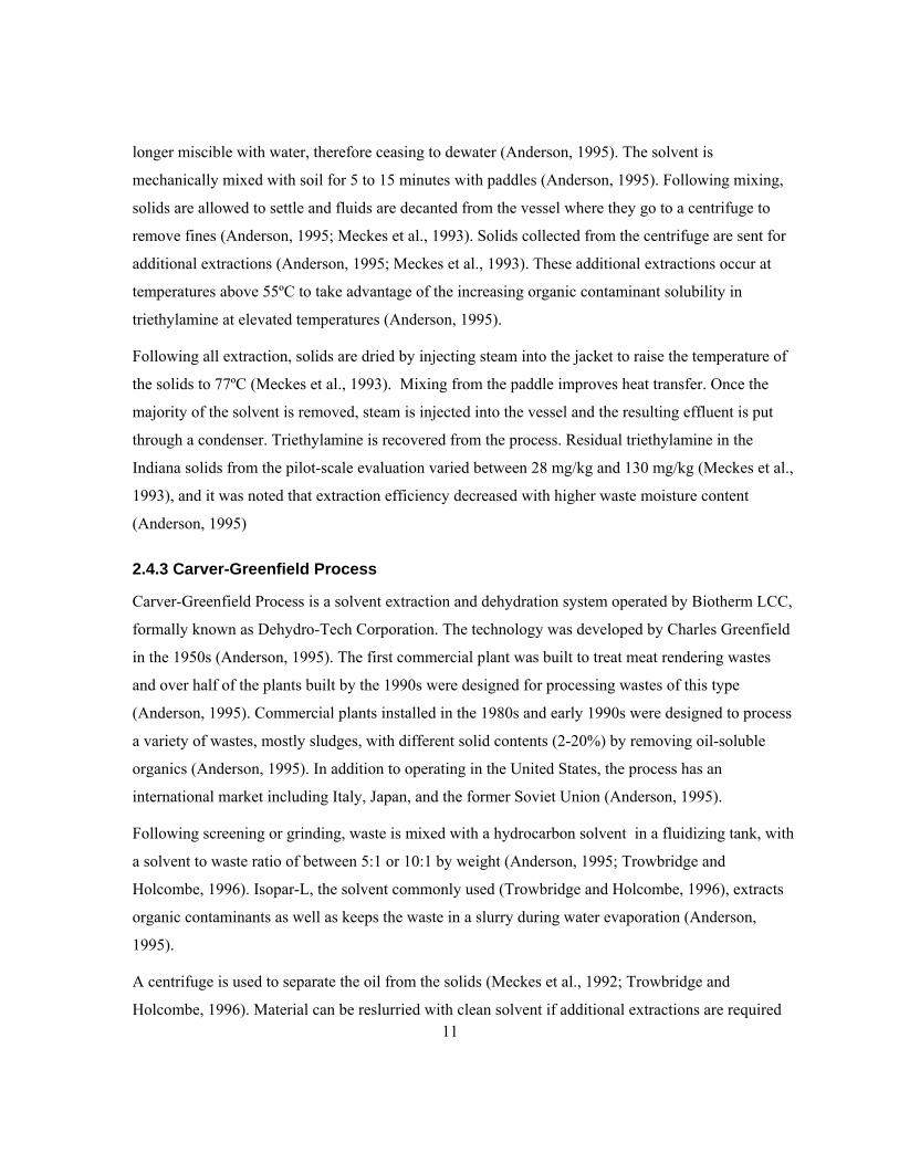
Dielectric constants are a measure of attraction between two poles and were examined for the solvents

under consideration (Table 2.3). It was suggested that the solvating abilities of an alcohol would

increase as the chain length grew (Forsey, 2007). Dielectric constants (and hence polarity) of alcohols

decrease as the chain length becomes longer therefore becoming more non-polar. At the same time,

the extensively chlorinated PCB congeners are more hydrophobic and Jakher et al. (2007) suggested

that as such it may be these more chlorinated PCB congeners that persist in weathered soil samples as

opposed to the lesser-chlorinated PCB congeners. It is the lesser-chlorinated congeners that are more

easily targeted by biodegradation, and are more soluble in water (Jakher et al., 2007). Looking solely

at degree of polarity, the above arguments would suggest that the solvent with the smallest dielectric

constant would be the best suited for extracting PCBs from soil. Jakher et al.’s findings support this

theory as they concluded that isopropyl alcohol had a better extraction efficiency than methanol

(2007). Isopropyl Alcohol was also selected by Dhol for PCB extraction in his thesis work (Dhol,

2005).

Unfortunately as the dielectric constant decreases, the solvents solubility in water decreases. This

becomes problematic when trying to extract PCBs from soils with higher moisture content. In these

cases, non-polar solvents are incapable of penetrating wet soils. In addition, dielectric constants may

vary with temperature (Lou et al., 1997).

2.5.3 Solvent Viscosity

Solvent extraction operators in colder climates claim to have witnessed noticeably increased solvent

viscosity in colder weather, increasing the amount of time required to fill and drain extraction bins,

15

thus increasing the overall operation time. For this reason, viscosity data from CRC Handbook of

Chemistry and Physics was examined (Figure 2.1) (Lide, 1998). Data were available for all of the

solvents not removed due to toxicity concerns.

Triethylamine, ethyl acetate and isooctane consistently have the lowest viscosity and the smallest rate

change as temperature decreases making them ideal solvent if only viscosity is considered (Figure

2.1). For the alcohols shown, their viscosities increase with increasing chain length.

The soil moisture content changes the viscosity of the solvent. For methanol, ethanol, 1-propanol,

and 2-propanol, an increased water content increases the solvent viscosity, however the rate change is

approximately the same (Lide, 1998) (Figure 2.2).

2.5.4 Solvent Freezing Point

Solvents used for solvent extraction must not freeze in Ontario winter temperatures and so freezing

points for potential alcohol solvents were considered (Table 2.4). Based on this data alone, only 2-

methyl-2-propanol was unsuitable for use in solvent extraction because it is solid at most of the

relevant temperature range. The other alcohols are liquid at relevant temperatures.

The moisture content of the soil changes the freezing point of the solvent. Freezing point data at

varying moisture contents for methanol, ethanol, 1-propanol, and 2-propanol are shown in Figure 2.3

(Lide, 1998). A moisture content of at least 50 % is necessary before the solvent/water mixture could

potentially freeze in Ontario winters (Figure 2.3). Fifty percent moisture content is above the water

saturation limit of a typical soil. Therefore the effect of soil moisture content on solvent freezing

should not dictate solvent selection.

2.5.5 Solvent Boiling Point

Another important consideration is the boiling point of the solvent as distillation is frequently used as

a solvent water separation technique, such as by CET Environmental Services in the Extraksol

Process (Anderson, 1995). Solvents having boiling points very similar to that of water, such as 1-

propanol or 2-butanol, are difficult to separate from water using this method. Since other separation

techniques are available, potential solvents should not be eliminated based on their boiling point.

Furthermore, solvents will only need to be separated from water if they are miscible with water. All

the alcohols in Table 2.4 are completely soluble in water with the exception of 1-butanol and 2-

butanol which have solubilities of 8.00 and 12.5 g/100 mL of water respectively (Streitwieser et al.,

16

1992). The non-alcohol solvents have suitable melting points with the exception of dimethyl

sulfoxide (Table 2.5).

Azeotropes were present amongst the potential solvents considered, and were those solvents that

when combined with water had different boiling points from that of pure solvent. Ethanol, 1-butanol,

2-butanol and ethyl acetate are all azeotropic mixtures with water (Lide, 1998) (Table 2.6). The

change in boiling point is largest for the two butanols.

A combination of polar and non-polar solvents may be preferred over a single solvent as discussed in

section 2.5.2. However, no azeotropes for binary combinations of the nine solvents were identified by

examining “Azeotropic Data for Binary Mixtures” in the CRC Handbook of Chemistry and Physics

(Lide, 1998).

2.5.6 Solvent Cost

Solvent cost for the nine solvents passing the toxicity, polarity, viscosity, and freezing and boiling

point screenings, was easily compared as most were available from the scientific chemical supplier

VWR as BDH Reagent Grade Solvents in 19L steel cans (Table 2.7). Triethylamine, 2-butanol and

isooctane were not available in the same volume and/or same grade which complicated the

comparison as cost can be dependent on both these factors. Overall, methanol was found to be the

cheapest, whereas isooctane the most expensive; however isooctane was only available in 2.5L

volume from VWR perhaps contributing to its higher cost.

2.5.7 Solvent Selection

Weights were applied to the solvent properties considered in order to rank the solvents (Appendix A).

The polar and non-polar solvents were considered separately. Toxicity was given the highest weight

for the polar solvents, followed by cost, while dielectric constant and recommendations were given

equal weights. For the non-polar solvents, the largest weight was assigned to toxicity, followed by

dielectric constant, and finally cost. The two highest ranking polar solvents were ethanol and

isopropyl alcohol. The two highest ranking non-polar solvents were isooctane and triethylamine.

These were therefore selected for use in laboratory experiments aimed at fulfilling the research

objectives.

17

2.6 Properties Controlling PCB Sorption and Desorption

Various properties control PCB absorption, adsorption and desorption to soil or sediments.

2.6.1 Soil Composition

Soil composition plays an important role in PCB sorption. Natural organic materials in soils and

sediments largely determine the sorption capacity of a soil and include humic substances,

biopolymers from which they were derived, lipids, proteins and lignin, kerogen, and combustion-

related black carbon or char materials (Huang et al., 2003). The organic matter in any given soil is a

function of climate, vegetation, topography, and parent material (Stevenson, 1982).

Humic substances are a large and generally the most abundant portion of natural organic materials in

soils and sediments (Weber et al., 2001). Carroll et al. (1994) described humic organic matter as a

complex of swollen and condensed polymer-type phases bound to mineral surfaces. They can be

classified into three groups: fulvic acid, humin, and humic acid (Huang et al., 2003; Stevenson, 1982).

Humic substances are believed to be the derived from biopolymers originating from lignin, a

fundamental part of plant cell walls (Pignatello et al., 2006).

Biopolymers are a group of molecules produced by living organisms which consist of repeating

structural units with large molecular mass. Included in this group are starch, proteins, peptides,

deoxyribonucleic acid, and ribonucleic acid. The role of biopolymers in the sorption of hydrophobic

organic chemicals (HOCs) such as PCBs is considered insignificant (Huang, Peng et al. 2003). Lipids

also play a small and often insignificant role in the sorption of hydrophobic organic chemicals,

despite their hydrophobicity, primarily because they comprise such a small fraction of soil/sediment

organic matter (Huang et al., 2003).

Kerogen is the dominant fraction of organic matter from sedimentary rocks, deriving from plant and

animals. Kerogen’s three-dimentional structure and many parallel sheets forming its aromatic nuclei

allow it to easily trap small hydrophobic organic solutes (Huang et al., 2003). It is insoluble both in

nonpolar or weakly polar organic solvents (Pignatello et al., 2006) and inorganic solvents.

Black carbon is often called soot or char depending on the form it manifests (Huang et al., 2003).

Black carbon does not contribute to the nonlinear and competitive sorption behaviour in bulk soils

(Pignatello et al., 2006). Pignatello et al. (2006) demonstrated that humic acids and humic precursors

18

free of black carbon sorb non-polar compounds nonlinearly and with competition when two solutes

are present.

Natural organic materials have been classified by some researchers as “soft carbon” or “hard carbon”.

A good review is provided by Allen-King et al. (2002). According to Huang et al. (2003) sorption of

HOCs into “soft carbon”, such as humic matter, occurs linearly whereas sorption on the “hard

carbon”, such as kerogen, follows adsorption and absorption or partitioning. The ratio of soft carbon

to hard carbon dictates whether sorption will occur linearly or nonlinearly (Huang et al., 2003). The

mineral fractions have minor roles in the sorption of hydrophobic organic contaminants, other than

having an effect on spatial distributions and arrangements of natural organic matter (Weber et al.,

2001).

The distributed reactivity model separates the sorption areas into three types. The first is comprised of

mineral sites. HOCs sorbed in this domain are done so by near-linear adsorption. The second type

comprises unstructured and swollen organic matter, and sorption is similar to that of solute

partitioning. The third type comprises a condensed yet unstructured fraction of natural organic matter.

Weber et al. (2001) propose that the third type of sorption area is responsible for the variety of

different adsorption processes due to different energy sites. They conclude that it is the third domain

that largely dictates the slower HOC sorption and desorption rates and accounts for the nonlinear

adsorption.

Carroll et al. (1994) observed both a rapidly desorbing labile component and a more slowly desorbing

resistant component in sediment. They hypothesized that the labile and resistant fractions are due to

the swollen (rubber-like) and condensed (glass-like) phases respectively of humic polymer in organic

matter (Carroll et al., 1994). They measured desorption of PCBs from sediments under various

conditions to explore the diffusion-controlling structure of the matrix.

The rubbery state is less condensed and has smaller cohesive forces than the glassy state. Sorption to

the rubbery state occurs by dissolution, where as sorption to the glassy state is from both dissolution

and hole-filling (Xing and Pignatello, 1997). The glassy domain is composed of rigid and condensed

organic matter and is responsible for slow desorption, nonlinear sorption, non-Fickian diffusion, and

sorption/desorption hysteresis (Schaumann and LeBoeuf, 2005). Rubbery domains are responsible for

the opposite: linear sorption and faster diffusion rates (Schaumann and LeBoeuf, 2005). Desorption

from soils with low total organic carbon and higher contents of minerals with high internal surface

19

areas will be influenced more by the entrapment of sorbed molecules within organic components

(Huang et al., 2003).

2.6.2 Soil Grain Size

There is a lack of consensus as to whether grain size influences PCB sorption. Carroll et al. (1994)

noted that PCB contamination in their samples was uniformly distributed between the different size

fractions with the exception of the 293-990 μm and <69 μm fractions. They concluded that particle

size did not impact the fraction of PCBs in the resistant fraction, and that silt and clay did not

appreciably affect the desorption of PCBs in their sample (Carroll et al., 1994). They also found that

while bar-milling did change the grain size distribution, it had no effect of PCB desorption in their 7

day experiments.

Many solvent extraction companies screen their soils to avoid treating large grain sizes. CF-Systems

screen soils to remove any materials greater than 0.64 cm (Meckes et al., 1997). Soil is pre-treated in

the Carver-Greenfield Process with separation and/ or grinding to ensure particle sizes less than 6 mm

(Anderson, 1995; Meckes et al., 1992). Sanivan Group’s Extraksol process treats nonporous solids up

to 0.6 m and porous solids up to 0.051 m (Anderson, 1995). The grain size limitations imposed by

these companies may be imposed by the mechanics of the operation and not the PCB contamination.

Wu and Gschwend (1988) considered grain size in earlier modeling work. They created a numerical

model capable of describing sorptive exchange in aqueous systems containing a range of particle

sizes and temporally varying solution conditions. Contradictory to the findings of Carroll et al.

(1994), their simulations showed that neglecting size distribution effects was a large source of

prediction error (Wu and Gschwend, 1988).

2.6.3 PCB Composition

In addition to soil composition and grain size, PCB composition plays a large role in PCB sorption.

Carroll et al. (1994) noted that diffusion coefficients decreased with increasing congener molecular

size and chlorine content in both the labile and resistant fractions (1994). They hypothesized that the

PCBs from the labile compartment (the more rapidly desorbing PCBs), would be more bioavailable to

anaerobes for reductive dechlorination producing ortho-substituted PCBs.

Lamoureux and Brownawell (1999) compared desorption from sediments containing compounds

representing tetra-, penta-, hexa-, and heptachlorobiphenyl. They discovered that the least

20

hydrophobic congener underwent the quickest rate change from fast to slow desorption and

consequently had the most sorption-resistant fraction. On the contrary, the most hydrophobic

congeners do not show a significant change in desorption rate over the 480 hours that the experiments

ran and had the smallest sorption-resistant fraction. Desorption of the majority of PCBs could be

described by a two-compartment model, consisting of an initially higher desorption rate followed by a

slower rate, however the highest molecular weight PCBs behaved differently (Lamoureux and

Brownawell, 1999). Pignatello et al. (2006) noted that the most hydrophobic compound among the

HOCs tested in their work also had the most nonlinear sorption.

2.6.4 Temperature

Temperature plays a role in the sorption of PCBs. Xing and Pignatello (1997) observed that the

linearity of sorption increased as the temperature increased however the effect of temperature on

sorption remains nonlinear (Pignatello et al., 2006). Diffusion rates also increase with increasing

temperature.

2.6.4.1 Glass Transition Temperature

The glassy or rubbery state of soil or sediment influences PCB sorption. The transformation from

glassy to rubbery state occurs at what is known as the glass transition temperature (Tg). Thermal

energy breaks noncovalent bonds allowing for this change of states (Pignatello et al., 2006).

A significant change in the heat capacity in a small temperature range typically reveals glass

transition temperatures (Schaumann and LeBoeuf, 2005). Earlier work identified the difficulty in

identifying single glass transition temperatures for whole soils and attributed this inability to

heterogeneity of the soil organic matter. This heterogeneity explained why there could be a range of

glass transition temperatures (Schaumann and LeBoeuf, 2005).

Pignatello et al. (2006) observed multiple transition temperatures in some macromolecules. The

humic acid sorbent extract from topsoil collected in Chelsea, Michigan, had the first transition

temperature between 3 and 6 ºC and is in a range that may influence sorption at colder temperatures

such as those encountered in Southern Ontario. They proposed that multiple transition temperatures

could be caused by regions of varying physical or chemical properties. The lower temperature glass

transition temperature is associated with side-chain mobility, where as the higher temperature glass

21

transition temperature is associated with main chain mobility (Pignatello et al., 2006). This glass

transition behavior was observed both in terrestrial and aquatic humic acids (Pignatello et al., 2006).

Schaumann and LeBoeuf (2005) suggest that the glass transition temperature may be impacted by

thermal or sample history. Glassy character is increased by a reduction in the mobility of side chains

caused by cross-linking. This change increases the glass transition temperature (Schaumann and

LeBoeuf, 2005). Glassy polymers can be in non-equilibrium if they were formed by cooling quickly

through the glass transition region. The glassy matrixes tend towards equilibrium by undergoing

structural relaxation, thus changing the macromolecular structure over time. The rate of structural

relaxation decreases with increasing glassy character. The rate is also a function of temperature, and

increases with increasing temperature when approaching the glass transition temperature (Schaumann

and LeBoeuf, 2005).

It may be that most glass transition temperatures in natural organic matter are above 20ºC (Table 2.8)

and that Ontario’s decreasing temperatures in the fall and winter months would not cause a transition

from rubbery to glassy state. However, the transition from glassy to rubbery state can also be

achieved by saturating the polymer with high concentrations of a swelling solvent (Xing and

Pignatello, 1997). This may be an important phenomenon during solvent extraction. The Fox-Flory

equation describes the glass transition temperature of a polymer/water gel and is given by

(2-2)

11 W WW P

g g g

C CT T T

−= +

where CW is the dimensionless water content, TgW is the glass transition temperature of water (136-

170K), and TgP is the glass transition temperature of dry polymer (Fox and Flory, 1954; Schaumann

and LeBoeuf, 2005).

Also, temperature affects sorption behaviour even below the glass transition temperature. As

temperature approaches the Tg, sorption tends to become more linear as a result of the solid becoming

more rubbery. The solid-phase dissolution also becomes more important than hole filling as the

temperature increases (Pignatello et al., 2006). Organosolv lignin showed nonlinear sorption below

Tg, however no consensus exists in literature regarding this issue (Pignatello et al., 2006).

22

2.6.4.2 Glass Transition Temperature & Moisture Content

Water can influence the glass transition temperature of a soil. It can reduce the overall glass transition

temperature by acting as a plasticizer when the water content is increased (Schaumann and LeBoeuf,

2005). Other studies also exist that report antiplasticizing properties of water (Schaumann and

LeBoeuf, 2005). Schaumann and LeBoeuf (2005) tested the hypothesis that water can act as a

plasticizer and an antiplasticizer in the same sample, and that the differences in observed glass

transition behaviours are due primarily to water. An air-dried peat sample was used for assessing

glass transition behaviour by varying water content and thermal history (Schaumann and LeBoeuf,

2005). When the transition temperature was plotted versus the water content, Schaumann and

LeBoeuf (2005) observed the maximum transition temperature occurred at a moisture content of 12%

even though dried samples subject to hydration reached a maximum moisture content of 24 ± 1%.

The minimum transition temperature occurred in water-free samples suggesting water was acting as

an antiplasticizer below a moisture content of 12% (Schaumann and LeBoeuf, 2005).

Schaumann and LeBoeuf (2005) observed the glass transition temperature of their initially air-dried

sample decreased continually with increasing hydration time. They noted the transition temperature

decreased at a slower rate than the rate of which the water content increased. The authors believe their

findings suggest that changes in temperature and water content can induce slow structural relaxation

processes in natural organic matter over periods of time as short as days. They identified three

processes of structural relaxation (Schaumann and LeBoeuf, 2005):

1) Classical glass transition behaviour. This behavior occurs in thermally pretreated and very low

water-content samples.

2) Decreased macromolecular mobility and decreased glass transition temperature caused by water

acting as an antiplasticizer. In this study, this occurred in peat samples at water contents below 12%.

3) Slow swelling from water uptake caused by water acting as a plasticizer. In this study, this

occurred in peat samples at water contents above 12%.

2.7 Modeling Sorption

Understandings of PCB sorption can aid in the understanding of PCB desorption. The simplest model

describing the partitioning of hydrophobic organic contaminants between aqueous phase and soils or

sediments is the linear partitioning model described by

23

(2-3)

e D eq K C=

where qe is the equilibrium solid-phase solute concentration in µg/g, KD is the partitioning coefficient

in mL/g, and Ce is the equilibrium aqueous-phase solute concentration in µg/mL (Huang et al., 2003;

Karickhoff, 1980). However the model assumes an excess of sites for hydrophobic organic

contaminant molecules to sorb which is not always the case. The Langmuir model describes site-

limited sorption by

(2-4)

1

oe

ee

Q bCqbC

=+

where Q0 is the maximal sorption capacity in ug/g, b is the solute-surface interaction energy-related

parameter in mL/ug, and qe and Ce are defined as in the linear partitioning model (Huang et al., 2003).

Although the model is simple, it is thought to be incorrect for hydrophobic organic contaminant

sorption by soils or sediments (Huang et al., 2003). Instead, a model often used for describing

sorption is the Freudlich model given by

(2-5)

ne F eq K C=

where KF is the Freudlich model capacity factor or Freundlich constant in mL/g, n is the

dimensionless isotherm linearity parameter, and qe and Ce are defined as in the linear partitioning

model (Huang et al., 2003; Pignatello et al., 2006).

Xing and Pignatello (1998) used the Freudlich model to investigate the effect of natural aromatic

acids on the adsorption of anthropogenic organic compounds in soil. Aromatic acids were selected

based on their similarity of structure and size to many organic contaminants. They screened eleven

different aromatic acids for their effect on sorption of 2,4-Dichlorophenol and discovered that

sorption did not occur linearly (n≠1) (Xing and Pignatello, 1998). Xing and Pignatello (1998)

showed there is direct competition between aromatic acid and PCB congener 2,4-dichlorophenol for

24

sorption sites. They observed a decrease in the sorption distribution ratio with the presence of

aromatic acids, although the decrease was not always statistically significant.

Pignatello et al. (2006) noted that the organic carbon adsorption coefficient decreased with increasing

Ce and the rate depended on n. The values for n and Ce varied greatly for humic acids from different

soils for the same hydrophobic organic contaminants. The Freudlich model continues to be used in

more recent PCB research (Pignatello et al., 2006; Teuten et al., 2007).

2.8 Modeling Desorption

Karickhoff proposed the two-box release model for desorption of nonionic organic compounds from

sediments (Karickhoff, 1980). The two-box release model encompasses both the labile and resistant

fractions and is given by

(2-6)

1 21 1(1 )k t k tt

o

M x e x eM− −= + −

where Mt is the amount of organic contaminant remaining at time t in µg, MO is the initial amount of

organic contaminants in µg, x1 is the labile fraction of organic contaminant, k1 is the first-order rate

constant for the labile fraction in 1/hours, k2 is the first-order rate constant for the resistant fraction in

1/hours, and t is the desorption time in hours (Carroll et al., 1994; Karickhoff, 1980). The slow

compartment represented a more condensed organic matter phase (Xing and Pignatello, 1997).

Another compartment model is the dual-mode model. It is a combination of both the linear partition

model and the Languir model. It states that the total sorption to soil or sediment organic matter is the

sum of sorption in both the dissolution and hole-filling domains, and agrees with the concept of both

glassy and rubbery polymer states (Xing and Pignatello, 1997; Xing et al., 1996):

(2-7)

1

( ) ( )1

oni i

pi i

S b CS S D S H K Cb C=

= + = ++∑

where S is the sorbed concentration in µg/g, S(D) is the sorbed concentration in the dissolution

domain in µg/g, S(H) is the sorbed concentration in the hole-filling domain in µg/g, Kp is the lumped

sorption coefficient in mL/g, C is the solute concentration in ug/mL, bi is the affinity constant in

25

mL/ug, Si is the capacity constant in ug/g, and n is the number of unique holes. Xing and Pignatello

(1997) generated data that supported the dual-mode model.

Similar to Karickhoff’s model, Fang and Al-Abed (2007) presented another compartment model to

describe desorption of hydrophobic organic compounds from soil and sediment:

(2-8)

...aq fast slowk t k t k ttaq fast slow

o

C F e F e F eC

− − −= + + +

where Co is the concentration of contaminant in the sediment at time zero in µg/g, Ct is the

concentration of contaminant in the sediment in µg/g at time t (hours), Faq is the fraction of the

contaminant present in the aqueous phase, Ffast is the fraction of the contaminant present in the fast

desorbing sediment compartment, Fslow is the fraction of the contaminant present in the slow

desorbing sediment compartment, kaq is the rate constant of the extraction of PCBs in the aqueous

phase in 1/hours, kfast is the rate constant of fast desorption in 1/hours, and kslow is the rate constant of

slow desorption in 1/hours (can vary with time as sediments age).

Carroll et al.’s (1994) experiments suggested that kinetics and not thermodynamics were limiting

PCB desorption from their samples. Valentin (2000) studied solvent extraction of PCB mass in soil

using ethyl acetate, methyl iso-butyl ketone (MIBK) and hexane over time. One of her studies

measured the amount of PCB mass removed in ethyl acetate using a 40:1 solvent volume to soil mass

ratio. Like Weber et al. (2001) Valentin found that the removal rate was greatest initially and

decreased until her last measurement at 1250 minutes (Figure 2.4). Her extraction data followed the

fast compartment of the desorption models described by Karickhoff (1980) and Fang and Al-Abed

(2007):

(2-9)

11

k tt

o

M x eM−=

where Mt, Mo, x1, k1, and t are described as in the two-box release model. Karickhoff (1980) suggested

that the chemicals in the labile phase are easily desorbed using solvents, however it is the resistant

phase that will take much longer (days) to desorb (Karickhoff, 1980). He also noted that is the ratio of

the two phases and the extraction time that will ultimately determine percent extracted.

26

Another model used to describe desorption is the radial intraparticle diffusion model which uses

measurable sediment and HOC properties (Wu and Gschwend, 1988). Lamoureux and Brownawell

(1999) attempted to fit desorption data to the model and found that although it accurately described

desorption for high-molecular weight PCBs, it did not for low molecular weight PCBs. This

conclusion confirmed research by Pignatello and Xing who found the model was unable to accurately

describe slow sorption (Lamoureux and Brownawell, 1999). Lamoureux and Brownawell (1999)

thought that the most likely explanation as to why the model did not accurately describe desorption of

the less hydrophobic compounds was that there are micropores within the sediment matrix that are

available to smaller compounds but not to larger compound, due to larger size and different shape.

Lamoureux and Brownawell (1999) thought it more likely that the smaller, least hydrophobic PCBs

be removed more quickly as they are more soluble, leaving behind a more hydrophobic and therefore

resistant PCB pool. However, results contradicted their hypothesis and showed that the more

hydrophobic fraction had the smallest desorption-resistant fraction.

27

Table 2.1. Composition of PCB Isomer Groups from Erickson (Erickson, 1993)

PCB Isomer Group Empirical Formula Percent Chlorine Number of Isomers

Monochlorobiphenyl C12H9Cl 9 3

Dichlorobiphenyl C12H8Cl2 32 12

Trichlorobiphenyl C12H7Cl3 41 24

Tetrachlorobiphenyl C12H6Cl4 49 42

Pentachlorobiphenyl C12H5Cl5 54 46

Hexachlorobiphenyl C12H4Cl6 59 42

Heptachlorobiphenyl C12H3Cl7 63 24

Octachlorobiphenyl C12H2Cl8 66 12

Nonachlorobiphenyl C12HCl9 69 3

Decachlorobiphenyl C12Cl10 71 1

Table 2.2. Examples of PCB octonol-water partition coefficients (Hawker and Connell, 1988)

PCB Congener Log Kow

2 - dichlorobiphenyl 4.46

2,2’,5’ - trichlorobiphenyl 5.24

2,2’,4,5’-tetrachlorobiphenyl 5.85

2,2’,5,5’-tetrachlorobiphenyl 5.84

2,2’,4,5,5’-pentachlorobiphenyl 6.38

2,2’,3,4,4’,5’-hexachlorobiphenyl 6.83

2,2’,3,4,4’,5,5’-heptachlorobiphenyl 7.36

decachlorobiphenyl 8.18

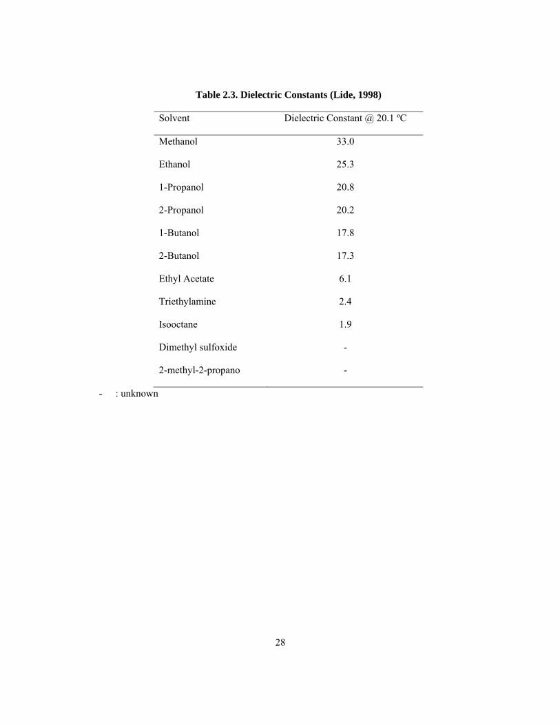
28

Table 2.3. Dielectric Constants (Lide, 1998)

Solvent Dielectric Constant @ 20.1 ºC

Methanol 33.0

Ethanol 25.3

1-Propanol 20.8

2-Propanol 20.2

1-Butanol 17.8

2-Butanol 17.3

Ethyl Acetate 6.1

Triethylamine 2.4

Isooctane 1.9

Dimethyl sulfoxide -

2-methyl-2-propano -

- : unknown

29

Table 2.4. Freezing and Boiling Points of Alcohols (Streitwieser et al., 1992)

Solvent Freezing Point (ºC) Boiling Point (ºC)

Methanol -97.8 65.0

Ethanol -114.7 78.5

1-propanol -126.5 97.4

2-propanol -89.5 82.4

1-butanol -89.5 117.3

2-butanol -114.7 99.5

2-methyl-2-propanol 25.5 82.2

Table 2.5. Freezing and Boiling Points of Non-Alcohols

Solvent Freezing Point

(ºC)

Boiling Point (ºC)

Dimethyl sulfoxide a 19 189

Ethyl acetate b -83.8 77.1

Isooctane a -107.3 99.22

Propane a -187.6 -42.1

Triethylamine a -115 89

a (Lide, 1998)

b (Mackay, 2006)

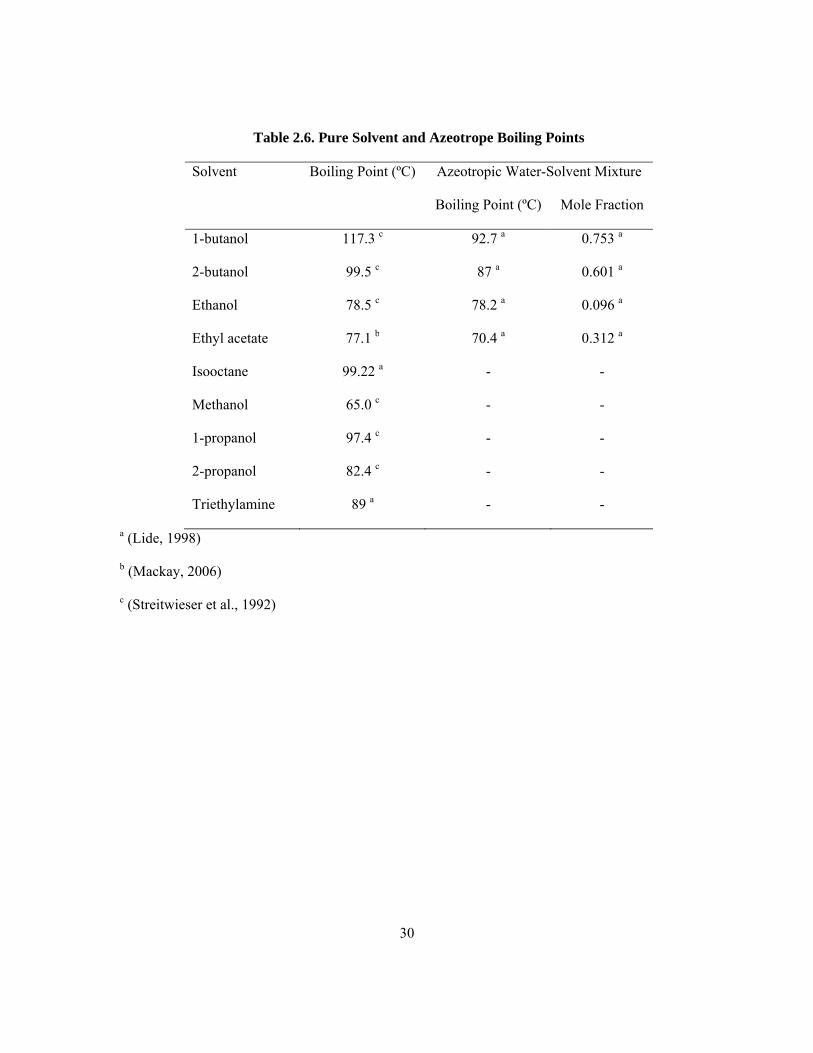
30

Table 2.6. Pure Solvent and Azeotrope Boiling Points

Solvent Boiling Point (ºC) Azeotropic Water-Solvent Mixture

Boiling Point (ºC) Mole Fraction

1-butanol 117.3 c 92.7 a 0.753 a

2-butanol 99.5 c 87 a 0.601 a

Ethanol 78.5 c 78.2 a 0.096 a

Ethyl acetate 77.1 b 70.4 a 0.312 a

Isooctane 99.22 a - -

Methanol 65.0 c - -

1-propanol 97.4 c - -

2-propanol 82.4 c - -

Triethylamine 89 a - -

a (Lide, 1998)

b (Mackay, 2006)

c (Streitwieser et al., 1992)

31

Table 2.7. VWR Solvent Prices

Solvent Volume (L) Unit Price

(Canadian$/L)

Methanol 19 3.81

2-Propanol, 99% 19 6.04

Ethanol, 95% 19 8.28

2-Butanol 208 10.35

Triethylamine 204 11.30

1-Propanol 19 13.19

1-Butanol 19 13.78

Ethyl Acetate 19 17.30

Isooctane 2.5 20.85

Table 2.8. Glass Transition Temperatures

Fraction Organic Matter Glass Transition Temp (Tg)

Lignins 68-83ºC a

Coals 99-125ºC, 307-359ºC b

a (Kadla et al., 2002)

b (Lucht et al., 1987)

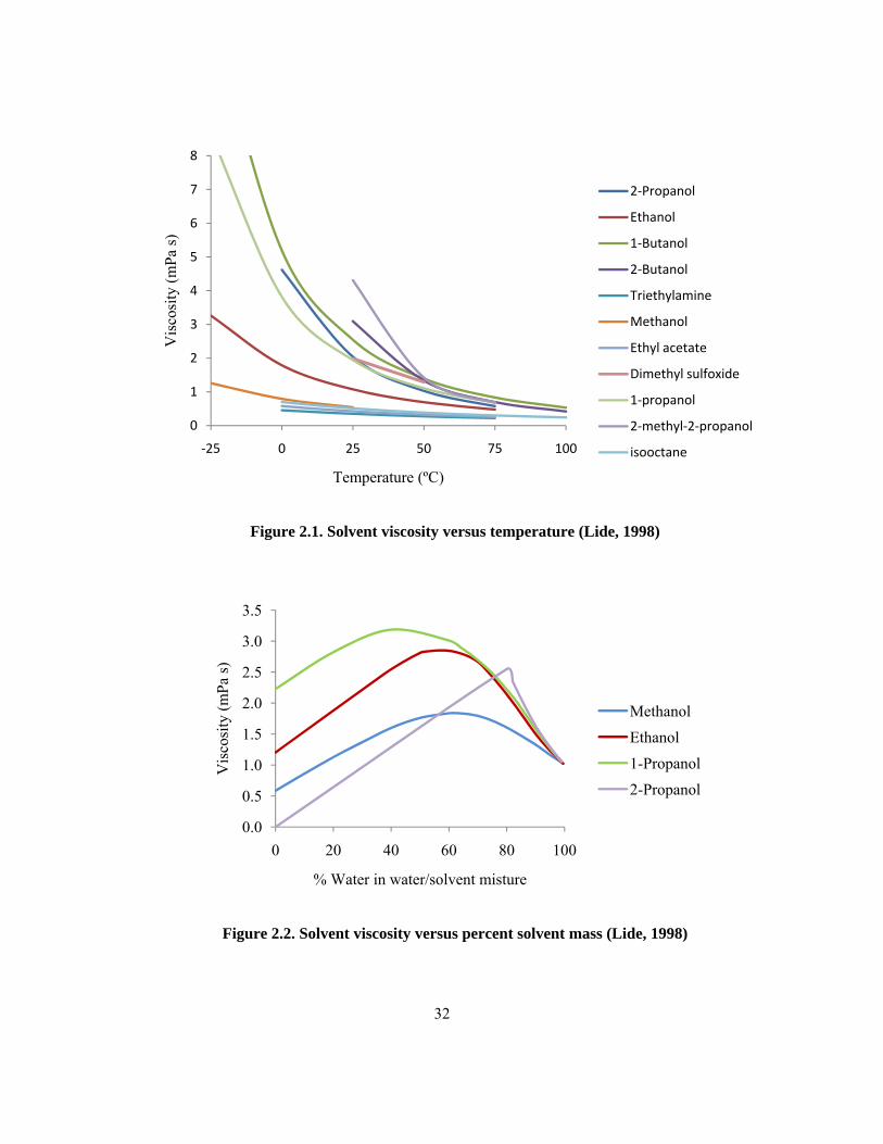
32

Figure 2.1. Solvent viscosity versus temperature (Lide, 1998)

Figure 2.2. Solvent viscosity versus percent solvent mass (Lide, 1998)

0

1

2

3

4

5

6

7

8

‐25 0 25 50 75 100

Vis

cosi

ty (m

Pa s)

Temperature (ºC)

2‐Propanol

Ethanol

1‐Butanol

2‐Butanol

Triethylamine

Methanol

Ethyl acetate

Dimethyl sulfoxide

1‐propanol

2‐methyl‐2‐propanol

isooctane

0.0

0.5

1.0

1.5

2.0

2.5

3.0

3.5

0 20 40 60 80 100

Vis

cosi

ty (m

Pa s)

% Water in water/solvent misture

Methanol

Ethanol

1-Propanol

2-Propanol

33

Figure 2.3. Solvent freezing points versus percent solvent mass (Lide, 1998)

Figure 2.4. PCB mass extracted with ethyl acetate over time (Valentin, 2000)

‐140

‐120

‐100

‐80

‐60

‐40

‐20

0

0 20 40 60 80 100

Free

zing

Poi

nt (º

C)

% Water in water/solvent mixture

Methanol

Ethanol

1‐Propanol

2‐Propanol

050

100150200250300350400450500

0 200 400 600 800 1000 1200 1400Mas

s of P

CB

in S

olve

nt A

fter t

reat

men

t (u

g)

Duration of First Extraction (minutes)

34

Chapter 3 Methods & Materials

3.1 Experimental Design

To meet the objectives of this research, the impact of elevated moisture contents and low temperature

on extraction efficiency was determined through a series of screening experiments using polar and

non-polar solvents at both 20ºC and 4ºC. It was hypothesized that improved extractions may be

possible with combinations of polar and non-polar solvents. Based on the results of these screening

experiments, a factorial experiment was designed using solvent combinations to further assess the

role of moisture contents and low temperatures. The role of PCB mass distribution among grain sizes

was also evaluated to see if optimization based on grain size separation is possible. Finally,

experiments were performed to generate data suitable for the development of a kinetic model that

incorporates key factors affecting solvent extraction.

3.1.1 Single Solvent Screening Experiments

Screening experiments were conducted to evaluate how extraction efficiency was dependent on the

soil moisture content. Fifteen grams of PCB contaminated air dried soil was added to 40 mL EPA

reactors and the moisture content was adjusted in each vial using Milli-Q water to either 0%, 5%,

10%, 15% or 20% w/w. After 24 hours, 15 mL of solvent was added to each reactor and the reactors

were placed on a mixer (30 RPM) for 24 hours. This 1g soil:1mL solvent ratio was comparable to that

used by Jakher et al. (2007). Following extraction, the reactors were centrifuged (1800 RPM, 5 min)

and the solvent decanted. The decanted solvent and the soil were then analyzed for PCB

concentration.

Isopropyl alcohol (polar), ethanol (polar), isooctane (non-polar) and triethylamine (non-polar) were

utilized as solvents based on the review discussed in Chapter 2. To evaluate the impact of low

temperatures on solvent extraction, extractions were also repeated at 4ºC for the polar solvents

(isopropyl alcohol and ethanol). The air dried soil had a residual moisture content (w/w) of 0.41 to

0.95% before the moisture content was adjusted (ASTM International, 2007). For simplicity this

residual moisture content is neglected in the following discussion.

35

3.1.2 Solvent Combination Experiments

A 24 factorial experiment (Johnson, 2000) was performed to evaluate combinations of both polar and

non-polar solvents at both high and low moisture contents. The factors investigated were choice of

polar solvent, choice of non-polar solvent, moisture content and temperature.

Reactors consisted of 40 mL EPA vials with 15 g of air-dried PCB contaminated soil, Milli-Q water

added to the desired moisture content, 7.5 mL of polar and 7.5 mL of non-polar solvents. The reactors

were mixed (30 RPM) for 24 hours before centrifugation (1800 RPM, 5 min) and decanting the

solvent. The polar and non-polar solvents were the same as those used in the screening experiments.

The decanted solvent and soil were analyzed for PCB concentration. During the factorial experiments

the solvents became separated in the reactors containing ethanol and isooctane at both the 5% and the

20% moisture content, as well as in the reactors containing isopropyl alcohol and isooctane at the

20% moisture content only (Figure 3.1 (a)). For these reactors, both layers of the decanted solvent

were analyzed for PCB mass separately and then summed. The volume of each layer was estimated

using digital images of the reactors and a ruler. It was assumed that the complete top layer was

decanted following centrifugation and available for analysis and that only a portion of the bottom

layer was lost during transfer. The controls next to the samples in Figure 3.1(b) contain 15 mL of

solvent and were employed to determine a height per volume conversion.

3.1.3 PCB Mass Distribution

Varying grain sizes were analyzed for PCB concentration. This analysis permitted an appraisal of

PCB mass distribution throughout the grain sizes. The analysis also aimed to relate PCB mass

distribution to organic content, determined using ASTM D2974-07a (ASTM International, 2007), and

fractional organic carbon (Churcher and Dickhout, 1987) as literature has indicated that these are

good tools for identifying where PCB mass resides (Allen-King et al., 2002). PCB concentration was

reported per mass of air dried sample instead of mass of dry sample as not enough sample remained

to determine the residual moisture content of each grain size grouping. The grain sizes examined are

listed in Table 3.1. There was not enough Dixie0707 soil available to create the same grain size

groupings as with the Dixie0208 soil.

36

3.1.4 Kinetic Experiments

Experiments were conducted to observe extraction kinetics. The rate of PCB mass removal from soils

using solvents is not well understood. The aim of these experiments was to collect significant data to

develop a kinetic model for predicting solvent extraction rates during field applications. These

experiments were performed using isopropyl alcohol, varying one parameter known to influence

solvent extraction rate at a time. The initial experiment assessed PCB mass extracted after 1, 3, 6, 24

and 48 hours respectively. Most of the extraction occurred in the first hours, so subsequent

experiments focused on collecting more early time data (0.5, 1, 3 and 3 hours). Thus PCB mass was

extracted until 24 hours only. All reactors consisted of 40 mL EPA vials containing 15 g of air-dried

PCB contaminated soil. Other design details for the experiments are shown in Table 3.2.

3.2 PCB Sample Origin

Past research has demonstrated that weathered PCB contamination is more difficult to remove than

synthetically prepared samples. Thus contaminated field samples from Southern Ontario, Canada

were employed. Two soil samples of approximately 10 kg were collected from stock piles on site.

Each was homogenized upon arrival at the lab. The first soil sample was collected in July 2007 and

labeled Dixie0707. The second was gathered in February 2008 and labeled Dixie0208. The

Dixie0707 soil was used for preliminary analysis while the Dixie0208 soil was utilized for the

majority of the experimental work in this research.

Grain size analysis allowed the classification of Dixie0707 soil as a silty or clayey sand according to

the British Soil Classification System and the Unified Soil Classification System (Craig, 2002)

(Figure 3.2 (a)). Dixie0208 soil was classified as a very silty or very clayey sand by the British Soil

Classification System or as a silty or clayey sand according to the Unified Soil Classification System

(Craig, 2002) (Figure 3.2 (b)).

All experiments used grain sizes less than 2.00 mm to ensure homogeneity among smaller samples

sizes unless otherwise specified. The specific gravity of the soil <2.00 mm was measured to be 2.68

g/cm3. Assuming a bulk density of 1950 kg/m3 (that of a well graded sand) then water saturation is

reached at a moisture content of 28.6% by weight.

37

3.3 PCB Analysis Procedures

3.3.1 Soil Extraction Methods

Soxhlet extraction (EPA Method 3540C) is the most reliable method for PCB removal from solids.

Unfortunately it is extremely time consuming requiring 16-34 hours per extraction (EPA, 1996a).

There are other problems associated with this method, including the risk of fire from unattended

samples. Soxhlet extraction was not selected as a result. Four other EPA methods were considered for

PCB extraction for quantification prior to selecting a suitable method (Table 3.3) (EPA, 2007a).

These methods were for semi volatile and nonvolatile organics.

Ultrasonic extraction (EPA Method 3550C) was appealing as it is employed by analytical labs such as

Maxxam Analytics in Mississauga, Ontario (Gripton, 2007). However, inquiries made to the US EPA

revealed problems with using this method for the soil type under consideration (Tisa, 2007). Other US

EPA methods were also eliminated based on the recommended concentration range, such as EPA

Methods 3541 and 3580 (Table 3.3).

Donnelly et al. (1996) evaluated PCB extraction using Soxhlet and the Dionex ASE ® 200

Accelerated Solvent Extractor (ASE200) (EPA Method 3545) and determined that both methods

produced high and reproducible recoveries. The ASE200 also used less solvent (Donnelly et al.,

1996). Furthermore, ASE200 holding times of 5 and 10 minutes produced the same outcome

(Donnelly et al., 1996). Although the concentration span identified by EPA Method 3545 did not span

the expected concentration of the samples (Table 3.3), the method appeared the most applicable due

to its simplicity and speed.

The ability of the ASE200 to extract higher PCB concentrations than those specified in EPA Method

3545 was assessed by comparing soil extractions from the ASE200 and Soxhlet (Table 3.4). Using

the ASE200, extractions were conducted on three sample sizes, including both larger and smaller

sample sizes than the 15 g of soil typically used. Although PCB concentrations differed considerably

depending on whether or not spike recovery (to be discussed in section 3.4) was applied (Table 3.4),

neither data reported statistically significant higher PCB concentrations with the Soxhlet method than

with the ASE200. As a result, EPA Method 3545 was deemed effective at extracting PCB mass from

the soil used in this research.

38

3.3.2 Analytical Soil Extraction

PCB mass was removed from soil samples using the ASE200 in accordance with EPA Method 3545A

(EPA, 2000a). Contaminated soil was packed into 33 mL stainless steel cells with Ottawa sand to fill

any remaining space in the cells. Glass fiber filters were positioned at both ends. HPLC grade hexane

and acetone were flushed through the cells in a 1:1 ratio (v/v). PCB mass was transferred into the

solvent from the soil under high temperatures and pressure, and collected into 60 mL EPA vials. The

solvent extract was then reduced to approximately 1 mL with the Dionex SE500 Solvent Evaporator

(SE500). The SE500 employed nitrogen gas at low pressure, approximately 5-20 kPa, a swirling

motion, and upper and lower heated blocks set to 25ºC.

3.3.3 Sample Clean-Up

The majority of PCB samples underwent sample cleanup prior to being run on the gas

chromatograph. Florisil cleanup was implemented with hopes that it would prolong the life of the gas

chromatograph column and detector as well as provide more accurate PCB concentration

measurements. The reduced solvent extract was passed through Florisil and sodium sulphate to

remove chlorinated hydrocarbons and pesticide residues, and water respectively. The extract was

diluted with HPLC grade hexane in the process. This procedure was comparable to the EPA Method

3620C (EPA, 2000b) column method and the approach employed by the Ontario Ministry of the

Environment (MOE) labs for PCB sample preparation (Ontario Ministry of the Environment, 2006).

A simple comparison was done at the beginning of the study to assess whether Florisil cleaup was

required for the samples. No interference was visually observed in samples not having undergone

Florisil cleanup, however, the cleanup was thought to prolong the life of the gas chromatograph

electron capture detector. The MOE PCB lab in Toronto, Ontario uses Florisil cleanup for their PCB

samples.

Similarly, sulphuric acid and permanganate cleanups were assessed at the beginning of the study in

accordance with EPA Method 3665A (EPA, 1996b). As with the samples having undergone Florisil

cleanup, no interferences were visually observed in the gas chromatoraphs not having undergone

cleanup. Thus these additional sample clean-up steps were not used.

Copper was used to remove sulphur interference and is employed by the MOE lab (Ontario Ministry

of the Environment, 2006). A known mass of copper was placed in the volumetric flasks used to

collect the sample after it had passed through the Florisil and sodium sulphate.

39

3.3.4 Gas Chromatograph Analysis

A Hewlett Packard G1530A gas chromatograph (GC) with an electron capture detector and Equity-

1701 column from Sigma Aldrich Canada was used to quantify the PCB mass in samples. A 1-2 µL

aliquot of PCB sample in hexane was injected into the GC where the congeners eluted at different

retention times depending on their mass. The types of Aroclors present in a sample were identified by

studying the pattern of chromatograph peaks and comparing them to the pattern of peaks from

Aroclor standards.

Although all common Aroclor standards were run on the GC with each sample set, only calibration

curves for the Aroclor known to be in the soil sample were created following its identification. The

Aroclor standards runs were prepared from more concentrated solutions or pure PCB obtained from

Sigma Aldrich Canada (Catalogue numbers: 48589, 48318, 90129R, 48591, 48588, 48586, 442463,

and 48585). Multiple calibration curves were created by plotting peak area versus concentration for

many of the characteristic peaks as described by EPA Method 8000 and EPA Method 8082 (EPA,

1996c; EPA, 1996d). The reported sample concentration is the mean concentration determined from

multiple peaks. Many samples were diluted so they fell within the calibration curve range prior to GC

analysis. As the samples injected into the GC were in hexane, the PCB concentration determined from

the calibration curves were in terms of mass per volume and were manipulated into concentrations in

terms of PCB mass per mass of dry soil.

Details of the GC settings are provided in Table 3.5. It should be noted that a longer final holding

time was used than was recommended by EPA Method 8082 due to preliminary analysis which found

carryover between samples. A 1:10 split injection was used.

The data presented in Chapter 4 represent the mean concentration of three replicate reactors along

with plus/minus one standard deviation between the triplicates. Two tailed t-tests evaluated the

statistical difference between the means at the 10% level of significance. Statistical outliers were

removed using Chauvenet’s Criterion (Kennedy and Neville, 1976). The data collected in the factorial

experiments underwent an analysis of variance (ANOVA).

3.3.5 Comparisons with Accredited Laboratories

Homogenized Dixie0208 air-dried soil samples (<2.00 mm grain size) were submitted to Maxxam

Analytics (Maxxam), ALS Laboratory Group (ALS) and the Ontario Ministry of the Environment

40

(MOE) for PCB concentration analysis as Aroclors (Table 3.6). The samples were submitted to

establish an accepted PCB concentration in the soil.

PCBs in hexane from extracting PCB mass from soil samples with the ASE200 was also submitted to

ALS and MOE to test for potential differences in the effectiveness of PCB extraction methods.

Results from the submitted PCB extract in hexane were converted from µg/L to µg/g to allow for

direct comparison with soil sample results (Table 3.7).

All three accredited laboratories reported different Aroclors for both the soil samples as well as the

PCB extracts submitted (Table 3.6 and Table 3.7). In addition, the concentrations varied greatly

between the various laboratories. Contaminated Dixie0707 soil submitted to Maxxam had been

reported as Aroclor 1260, whereas the Dixie0208 soil was reported as Aroclor 1248. Although it is

possible to have different types of PCB contamination on a given site, it was expected that the

Dixie0707 and Dixie0208 soil samples would contain the same Aroclor type as the samples were

taken from the same site. The PCB concentrations in the soil as determined from the submitted soil

were 925 ± 100 µg/g (ALS), 637 ±164 µg/g (MOE), and 320 ± 26 µg/g (Maxxam). The submitted

solvent samples resulted in lower concentrations than the soil samples; 745 ±70 µg/g (ALS) and 555

±59 µg/g (MOE).

The Dixie0208 soil was analyzed as both Aroclor 1248 and 1242 and compared with the reported

concentrations from the accredited labs (Table 3.6). The internal and accredited laboratory analysis

showed that the reported concentration depended on the Aroclor identified. Triplicates of sieved air-

dried soil analyzed as Aroclor 1248 were most similar to the concentrations reported by MOE at 606

± 28 µg/g, where as soil analyzed as Aroclor 1242 approximately one month later had concentrations

most similar to those reported by ALS at 1155 ± 64 µg/g. It was decided that the Dixie0707 and

Dixie0208 soil should be consistently analyzed only for Aroclor 1248 over the course of the study to

allow for direct comparisons between experiments.

3.4 QA/QC

Decanted solvent and soil samples were spiked with a known volume and concentration of

decachlorobiphenyl (DCB) to check for recovery as recommended in EPA Methods 8000 and 8082

(EPA, 1996c; EPA, 1996d). Decachlorobiphenyl is the heaviest of the 209 congeners and has the

longest retention time on the gas chromatograph, allowing it to be easily distinguished from the

41

common Aroclors and congeners. At times the DCB recovery was very poor and/or varied widely

between samples (Table 3.8).

Experimental data was corrected for recovery prior to data analysis. The DCB recovery was not

applied to the data from the experimental extraction done with isooctane at 20ºC since the DCB

calibration curve was poor and the recovery was in all cases over 1000%. Where DCB recovery

changed the outcome, both uncorrected data and data corrected for DCB recovery are presented. In

addition to spiking each sample with DCB, clean solvents were set up as controls as a check that no

PCB mass was introduced through the solvents used or transferred from vial to vial over the course of

the experiment.

42

Table 3.1. Grain Sizes Assessed for PCB Mass Distribution

Soil ID Grain Size (mm) Sieve Number

Dixie0208 <0.425

0.425 – 0.85

0.85 – 2.00

2.00 – 4.75

> 4.75

Passing 40

Retained on 40

Retained on 20

Retained on 10

Retained on 4

Dixie0707 0.075 – 0.25

0.25 – 2.00

2.00 – 19.05

> 19.05

Retained on 200

Retained on 60

Retained on 10

Retained on ½ inch

Table 3.2. Kinetic Experiment Design

Parameters Experiment 1 Experiment 2 Experiment 3

Soil:Solvent ratio (g:mL) 1:1 1:0.75 1:1

Temperature (ºC) 20 20 4

Grain size (mm) <2.00 <2.00 <2.00

Moisture Content (%wt) 5 5 5

43

Table 3.3. EPA Methods Considered for PCB Extraction for Quantification Purposes

Method No. Extraction Type Concentration

Range (µg/g)

Notes

3540C Soxhlet Extraction None listed Lengthy extraction: 16-24 hrs (EPA, 1996a)

The typical method used (Tisa, 2007)

3541 Automated

Soxhlet Extraction

1-50 Shorter extraction time than Method 3540C

(EPA, 1994)

3550C Ultrasonic

Extraction

Low

concentration

method: <=20

Medium/high

concentration

method: >20

Not recommended for PCB extraction and

considered less efficient that the other methods

(EPA, 2007a)

“May not be as rigorous” as the other methods

(EPA, 2007b)

Advised against its use for fine-grain sandy

soils (Tisa, 2007)

Many states are no longer allowing this method

for extraction of PCBs in their QAPP programs

(Tisa, 2007)

3580 Solvent Dilution > 20 000 Advised against its use for fine-grain sandy

soils (Tisa, 2007)

3545A Pressurized Fluid

Extraction (ASE)

(Heat & Pressure)

0.001 – 1.400 It may be applicable to samples containing

higher concentrations than specified range

(EPA, 2000a)

For lower concentration, sandy soils, the

method may work fine (Tisa, 2007)

44

Table 3.4. Comparisons between analytical soil extraction methods

Analytical

Extraction Method

Sample Size

(g)

PCB Concentration (µg/g)

Corrected for spike No spike correction

Soxhlet 10 577 ± 27 827 ± 29

ASE200 30 706 ± 63 887 ± 168

15 2557 ± 1748 803 ± 77

7.5 3012 ± 1385 986 ± 171

± Standard deviation

Table 3.5. Gas Chromatograph Settings (Adapted from EPA Method 8082 Table 2)

Parameter Recommended Setting

(EPA, 1996d)

Setting Used

Carrier Gas (Helium) 5-7 mL/min 4.4 mL/min

Makeup Gas (Nitrogen) 30 mL/min 30 mL/min

Injector Temperature 250ºC 250ºC

Detector Temperature 290ºC 290ºC

Initial Temperature 150ºC, hold 0.5 min 150 ºC, hold 0.5 min

Temperature Program 150ºC to 270ºC at 5ºC/min 150ºC to 270ºC at 5ºC/min

Final Temperature 270ºC, hold 10 min 270ºC, hold 15.5 to 25.5 min

Injection Volume 2 µL 1-2 µL

45

Table 3.6. PCB Concentrations in Soil Reported by Various Laboratories

Laboratory Aroclor Replicate PCB Concentrations (µg/g)

ALS 1242 950, 815, 1010

MOE 1248, 1254, 1260 332, 830, 676, 658, 656, 672

Maxxam 1248 290, 340, 330

UW 1248 629, 575, 615

UW 1242 1150, 1094, 1222

Table 3.7. PCB Concentrations in Hexane Reported by Accredited Laboratories

Laboratory Aroclor Triplicate PCB Concentrations (µg/g)

ALS 1242 822, 685, 728

MOE 1248, 1254, 1260 610, 562, 492

46

Table 3.8. DCB Recovery for each experiment

Solvent or Experiment Temperature Matrix Min Recovery (%) Max Recovery (%)

Isopropyl Alcohol 20ºC Decant 94 126

Isopropyl Alcohol 20ºC Soil 50 123

Isopropyl Alcohol 4ºC Decant 65 70

Isopropyl Alcohol 4ºC Soil 85 107

Ethanol 20ºC Decant 87 234

Ethanol 20ºC Soil 39 238

Ethanol 4ºC Decant 108 112

Ethanol 4ºC Soil 93 103

Isooctane 20ºC Decant 1989 2477

Isooctane 20ºC Soil 1080 2027

Triethylamine 20ºC Decant 98 120

Triethylamine 20ºC Soil 67 108

23 Factorial 20ºC Decant 102 117

23 Factorial 20ºC Soil 63 148

23 Factorial 4ºC Decant 99 111

23 Factorial 4ºC Soil 100 118

PCB Distribution– Dixie0208 Soil/ Rocks 29 137

PCB Distribution-Dixie0208 repeat Soil/ Rocks 74 194

PCB Distribution– Dixie0707 Soil/ Rocks 68 160

47

(a) (b)

Figure 3.1. (a) Images of ethanol and isooctane reactors following 24hr extraction, (b) Image of

reactors used to determine volume of solvent layers (isopropyl alcohol and isooctane at 20%

moisture content)

Solvent 1

Solvent 2 Soil

Isooctane Control

IPA Control

15 mL

15 mL

48

Figure 3.2. Grain Size Analysis of (a) Dixie0707 Soil and (b) Dixie0208 Soil

0102030405060708090

100

0.001 0.01 0.1 1 10

Perc

ent S

mal

ler (

%)

Grain Size (mm)(a)

0102030405060708090

100

0.001 0.01 0.1 1 10

Perc

ent S

mal

ler (

%)

Grain Size (mm)

(b)

49

Chapter 4 Results and Discussion

Chapter 4 discusses mass balance considerations, presents the results from the screening and factorial

experiments, and discusses the effects of moisture content, solvent choice, temperature, and grain size

on PCB extraction. A kinetic model is presented based on the results from the kinetic experiments.

4.1 Mass Balance Considerations

The initial mass of PCBs in the soil prior to the experimental extractions was assumed equal to the

PCB mass in the controls, however the soil sample used was a natural weathered sample and was

difficult to effectively homogenize as shown by the variability between replicates (Table 3.6 and

Table 3.7). Therefore the initial concentrations in some of the test reactors may have been greater

than in the controls. The data collected indicate that the sum of the mass of PCBs extracted by solvent

and the mass of PCBs remaining in the soil following the experimental extraction was greater than the

mass in the controls (Table 4.1). The inability to close the mass balance is likely due to a combination

of factors.

The PCB concentration remaining in the soil may be overestimated as not all the solvent containing

PCB mass is removed from the soil when it is decanted following an experimental extraction. For

example, in the 20ºC factorial experiment, 28 to 36% of the initial total weight of liquid remained in

the soil after the solvent was decanted. This is typical for all the experiments. Subtracting the mass of

PCBs in the solvent remaining in the soil from the mass of PCBs determined to be in the soil often

leads to a negative value. Some of this solvent containing PCB mass is removed from the soil during

preparation for extraction with the ASE200 but it is difficult to quantify.

It is possible that a more complete extraction may occur using the ASE200 following an experimental

solvent extraction than without it (as was the case with the controls), contributing to the presence of

more mass in the two phases (solvent and soil) following the experimental extraction than determined

in the controls. The experimental extraction may act as a type of pre-treatment allowing for a more

complete extraction when the soil is then put through a second extraction using the ASE200.

50

Different solvents may preferentially extract certain congeners. No preferential extraction was

visually noted from examining the gas chromatographs but analyzing the samples in terms of

Aroclors instead of congeners may be overestimating the total PCB concentration in the sample.

As there is more uncertainty associated with the PCB mass in the remaining soil, the decanted solvent

data is considered more accurate. The soil data is presented for completeness.

4.2 Moisture Content Effects on Solvent Extraction

4.2.1 Polar Solvents: At Room Temperature

The decanted solvent data indicated that the best extraction with isopropyl alcohol at 20ºC was

achieved at 5% moisture content (Figure 4.1(a)). However, the least PCB mass remained in the soil at

the 20% moisture content, indicting a different optimal moisture content (Figure 4.1 (b)). Since the

decanted solvent and soil data were contradicting and the optimal moisture content identified with

either data set was not statistically significant, the experimental extraction using isopropyl alcohol at

20ºC was repeated. The second set of extractions confirmed the optimal extraction occurred at a

moisture content around 5% (Table 4.2 and Figure 4.1(c)). A DCB spike was not added so these data

were not corrected for DCB recovery.

The optimal extractions using ethanol at 20ºC occurred at 5% or 15%, depending on whether or not

the data were corrected for DCB recovery (Table 4.2). With the corrections applied, the optimal

extraction occurred at 5% moisture consistent with isopropyl alcohol (Figure 4.2 (a)). When the data

was not corrected for DCB recovery, the optimal extraction occurred at 15% moisture content (Figure

4.2(b)). The DCB corrected data showed that the lowest PCB concentration remained in the soil at

20% moisture content (Figure 4.2 (c)), and the lowest PCB concentration remained in the soil at the

0% moisture content when the uncorrected data were examined (Figure 4.2 (d)). The data presented

for ethanol is inconclusive and the optimum depends on whether DCB correction is applied or not.

Also, the soil data does not support the findings based on the decanted solvent data.

Isopropyl alcohol extracted 70 to 78% of the PCB mass at 20ºC with the highest percent mass

extracted at 20% moisture content and the lowest at 0% moisture content (Figure 4.3). However, none

of PCB percent mass extracted were statistically different from one another for the range of moisture

contents explored. Ethanol extracted 61 to 71% of the PCB mass at 20ºC, and similarly to isopropyl

alcohol, the highest extraction occurred at the 20% moisture content, however only the percent mass

51

extracted at the 0% and 20% moisture contents were statistically different from one another (Figure

4.3).

The 0% moisture content isopropyl alcohol reactors were cloudier than the others (Figure 4.4 (a)).

This was again observed when the experiment was repeated with the same conditions, however the

5% moisture content reactors, were also much darker than the rest of the reactors the second time

(Figure 4.4(b)). The darker and cloudier colour could be from the extraction of organic matter since

organic matter is responsible for the dark colour in many soils (Stevenson, 1982). The 0% moisture

content ethanol reactors were opaque and dark in colour (Figure 4.5 (a)).

4.2.2 Polar Solvents: At Lower Temperatures

The decanted solvent from the experimental extraction with isopropyl alcohol at 4ºC showed the

extraction efficiency increasing as the moisture content increased until the optimal extraction at

moisture content of 15% (Figure 4.1(d)). The soil at 15% moisture content had more PCB mass

remaining in it than at 20% moisture content, contradicting the decanted solvent data. The

concentrations at 15% and 20% moisture content were statistically different (Table 4.2).

The optimal extraction using ethanol at 4ºC occurred at 5% moisture content as indicated by the

decanted solvent data (Figure 4.2(e)). In general, where the decanted solvent indicated higher PCB

concentrations (Figure 4.2 (e)), lower PCB concentrations remained in the soil (Figure 4.2 (f)). This

result was expected given the assumption that the initial PCB concentration in the soil samples was

uniform.

The average percent of PCBs removed with isopropyl alcohol at 4ºC ranged from 73 to 83 %, with

the highest percentage removed at both the 15% and 20% moisture contents (Figure 4.6 (a)). The

greatest percent extraction with ethanol at 4ºC was 84% and occurred at a moisture content of 0%

(Figure 4.6 (b)).

The trend observed at 4ºC with isopropyl alcohol was different from that observed during the 20ºC

experiments where the optimal extraction occurred at lower moisture content. The optimal moisture

content was consistent between both 4ºC and 20ºC for the decanted ethanol data using the DCB

corrected data at 20ºC (Table 4.2).

The reactors from the extraction at 4ºC with isopropyl alcohol and with ethanol appeared similar to

those at 20ºC. The 5% moisture content isopropyl alcohol reactors were darker and cloudier than the

52

others at 4ºC like the repeat extraction at 20ºC (Figure 4.4 (b), (c) and (d)). The darkest and most

opaque ethanol reactors at 4ºC corresponded with 0% moisture content; however, the 5% moisture

content reactors were not as dark as compared to the extractions performed at 20ºC (Figure 4.5 (b)).

The dark colour extracted at 5% moisture content with isopropyl alcohol and at 0% moisture content

with ethanol was present regardless of temperature.

4.2.3 Non-polar solvents: At Room Temperature

It was hypothesized that increased water content would hinder the extraction with non-polar solvents

giving optimum moisture content at 0%. The decanted isooctane indicated that the best extraction

achieved with isooctane was at the lowest (0%) and highest (20%) moisture contents (Figure 4.7 (a)).

Both these means were not statistically different from one another (Table 4.3). The residual PCB data

from the isooctane soil extraction showed the lowest amount of PCBs remaining in the soil at the 0%

moisture content (Figure 4.7(c)), suggesting that the highest extraction with isooctane did indeed

occur at 0% moisture content. Neither the decanted isooctane data nor the isooctane soil data has been

corrected for DCB recovery since the DCB calibration curve was not usable for this experiment.

The decanted triethyamine data indicated that the amount of PCBs extracted increased as moisture

content increased and the best extraction was achieved at the highest (20%) moisture content (Table

4.3 and Figure 4.7 (b)). The soil data from the triethylamine extraction supports the decanted

triethylamine results and indicates that the highest mass of PCBs remained in the soil with 0%

moisture content and the lowest remained in the soil with 20% moisture content (Table 4.3 and Figure

4.7 (d)).

The percent of PCB mass extracted ranged from 66 to 84% with isooctane, with the highest extraction

efficiency corresponding with the extraction at 0% moisture content (Figure 4.8 (a)), and from 81 to

90% with triethylamine (Figure 4.7 (d)).

The two non-polar solvents, both clear initially, changed appearance during these extractions. Unlike

the polar solvents, isooctane became increasingly darker as the moisture content in the reactors

increased (Figure 4.9 (a)). The decanted triethylamine was consistently very dark except for the 0%

moisture content reactors, where the least mass of PCBs was extracted (Figure 4.9 (b)).

53

The decanted triethylamine data contradicted the hypothesis. The different optimal moisture contents

between the two non-polar solvents studied suggests that the optimal moisture content is not dictated

strictly by polarity, and so no general conclusions can be drawn about non-polar solvents.

4.3 Solvent Combination Experiment

The conditions for the optimal extractions were the same at both 4ºC and 20ºC. The decanted solvent

data indicated the best PCB extraction was achieved at 20% moisture content using ethanol and

triethylamine in combination (Figure 4.10(a) and (b)). At 4ºC, the optimal extraction was not

statistically different from that with isopropyl alcohol and triethylamine at 5% moisture content. The

soil data contradicted the decanted solvent data, except for the ethanol and isooctane combinations

(Figure 4.10(c) and (d)).

The extraction efficiencies were above 80% for all solvent and moisture combinations at 20ºC and

4ºC except for the ethanol and isooctane combination at 5% moisture content (Figure 4.11). The

percent PCB mass extracted showed the best extraction at 4ºC was achieved with the isooctane and

ethanol combination at 20% moisture content, which differs from the result obtained by looking at the

decanted solvent data only.

When isopropyl alcohol was used in combination with either non-polar solvent, more PCB mass was

extracted at 5% than at 20% moisture content (statistically significant with triethylamine at 20ºC, and

statistically significant with isooctane at 4ºC). The reverse was true when ethanol was used in

combination with either non-polar solvent (statistically significant in all scenarios).

The optimal moisture content when ethanol was used in combination with a non-polar solvent was the

opposite of what was observed when ethanol was used on its own (Figure 4.2 (e)), but the same as

triethylamine on its own (Figure 4.7 (b)). It appears that triethylamine has the stronger influence when

ethanol and triethylamine are used in combination.

At 4ºC, the combinations which included triethylamine in general outperformed those using

isooctane. This observation was statistically significant except among the mean concentrations

extracted at 5% moisture content using isooctane and isopropyl together, and using triethylamine and

ethanol together. At 20ºC, triethylamine outperformed isooctane when it was used in combination

with the same polar solvent at the same moisture content except with isopropyl alcohol at 5%

moisture content, where the isooctane and isopropyl alcohol combination at 5% moisture content

54

significantly extracted more than triethylamine and isopropyl alcohol together at 5% moisture

content.

4.3.1 ANOVA Results for 24 Factorial Experiment

When an ANOVA was performed on the 4ºC and 20ºC decanted solvent data treated as one 24

factorial experiment, the choice of polar solvent, the choice of non-polar solvent and temperature

were identified as significant main effects. The significant interactions were between choice of polar

solvent and choice of non-polar solvent, and between moisture content and choice of polar solvent

(Table 4.4).

All the main effects were significant when the ANOVA was performed on the percent removed data

(Table 4.5). Five interactions were significant: between choice of polar solvent and choice of non-

polar solvent, between choice of polar solvent and temperature, between choice of polar solvent and

moisture content, between choice of non-polar solvent and moisture content, and between choice of

polar solvent, choice of non-polar solvent and moisture content.

Different ANOVA outcomes should not appear whether the analysis is conducted on data from the

decanted solvent or the percent removed. The difference lies with the PCB mass that remained in the

soil following the experimental extraction, as the concentrations in the soil did not support the

decanted solvent data and may be less reliable as discussed in Section 4.1. Table 4.4 should be

considered more correct due to the errors involved in calculating the PCB concentration in the soil.

4.4 PCB Mass Distribution

PCB mass distribution was assessed amongst grain sizes. This was done with both Dixie0208 and

Dixie0707 soil.

4.4.1 PCB Mass Distribution in Dixie0707 Soil

PCB mass was not evenly distributed amongst the grains sizes in the Dixie0707 soil and the highest

mean PCB concentration was found in the 2 – 19.05 mm grain size range (Figure 4.12 (a)). The

darkest extract from the ASE200 extraction corresponded with this grain size range (Figure 4.13),

suggesting that PCBs were found where the most organics resided.

55

4.4.2 PCB Mass Distribution in Dixie0208 Soil

Like the Dixie0707 soil, PCB mass was not evenly distributed amongst all the grain sizes in the

Dixie0208 soil. The highest mean PCB concentration was found in the smallest grain sizes (<0.425

mm) when DCB recovery was applied, but in the 0.85 – 2.0 mm grain size range without DCB

recovery corrections (Table 4.6 and Figure 4.12(b) and (c)). The experiment was repeated, accidently

excluding grain sizes less than 0.425 mm (Figure 4.14 (a)). Similar to the first effort (Figure 4.12(b)),

the highest mean PCB concentration in the range studied resided in the 0.85 -2 mm grain size range

(Table 4.6 and Figure 4.12(c)). Unfortunately no conclusions could be drawn as to whether the

highest PCB concentration was in the less than 0.425 mm grain size or the 0.425 – 0.85 grain size

range. The results between the two soil types could not be directly compared as the 0.85 to 2.00 mm

grain size range only accounted for 21% of the 0.25mm to 2mm grain size range analyzed in the

Dixie0707 soil.

Although PCB mass was unevenly distributed, the congeners present in the Dixie0208 soil were

evenly distributed amongst the grain sizes. This was determined by assessing pattern consistency

between sample chromatographs and it appeared that each grain size had the same signature.

It was thought that the uneven distribution of PCB mass amongst grain sizes may be related to soil

organics in the grain size groupings and so each grain size range was analyzed for ash content and

therefore organic content (Figure 4.15 (a)). The mean organic content ranged between 1.5 and 2.8%

by weight for the different grain sizes. The highest organic content corresponded with the 2.00 to 4.75

mm grain size range, and therefore not where the highest concentration of PCBs was found (with or

without DCB recovery corrections). Although this result was not expected, the highest concentration

of organic content also had the largest standard deviation (0.49%) and was not statistically different

from that of the 0.85 to 2.00 mm grain size range which contained the highest concentration of PCBs

without DCB recovery corrections. It is however statistically significant from the <0.425 mm grain

size range which contained the highest concentration of PCBs with DCB recovery corrections

applied.

In a further attempt to relate PCB mass distribution to organic content, the same grain sizes were

analyzed for percent fraction organic carbon (FOC) by weight. The results showed the amount of

organic carbon decreased as the grain sizes increased (Figure 4.15 (b)). The grain size where the

highest concentration of PCBs was found did not correspond with the grain size with the highest

56

percent of fractional organic carbon. The total fraction organic carbon for the Dixie0208 soil was

estimated to be 1.6% by weight based on the fractional organic carbon results of the grain size

groupings and the results from the grain size analysis. While the FOC content did not correspond with

PCB mass, the organic content results did.

As a final check, the PCB mass extracted from the grain size groupings was summed after accounting

for the fraction that each grain size represented in the initial sample. The total PCB mass in the

complete soil sample was 16.4 ± 4.0 mg, (10.1 ± 1.3 mg without DCB recovery), and the total PCB

mass in the <2.00 mm grain size, the grain size used in all the screening and factorial experiments,

was 14.2 ± 3.7 mg, (8.5 ± a.0 mg without DCB recovery). This is not too dissimilar from the PCB

masses in the controls from the previous experiments however they do represent a large range (Table

4.1).

4.5 Effects of Moisture Content, Solvent Choice, Temperature and Grain Size on PCB Extraction

The solvent extractions conducted with polar solvents at 20ºC are inconclusive due to the lack of a

statistically significant difference and contradicting results whether DCB recovery was applied or not.

The solvent extractions conducted with the polar solvents at 4ºC are however more conclusive:

Isopropyl alcohol achieved the best extraction at the highest moisture contents (15-20%) while

ethanol had the best extractions at the lower moisture content (0-5%) (Table 4.2). The ANOVA on

the solvent combination experiments confirmed there is interaction between moisture content (5%

versus 20%) and choice of polar solvent (isopropyl alcohol versus ethanol). Ethanol and isopropyl

alcohol consistently had opposing optimal moisture contents when in combination with a non-polar

solvent at either 20ºC or 4ºC.

The unreliable DCB recovery values made numerical comparisons between the experiments

untrustworthy so it was difficult to assess if either ethanol or isopropyl alcohol achieved better

extractions. While the percent extracted showed that a better extraction was achieved with isopropyl

alcohol at 20ºC than with ethanol, and that similar percents were extracted with both solvents at4ºC,

the values take into account the PCB concentration remaining in the soil which is unreliable as

discussed in Section 4.1.

57

The solvent extractions at higher soil moisture contents (15-20%) were shown to be optimal when

using triethylamine as the solvent (Table 4.3). Isooctane achieved optimal extractions at both the

extreme moisture contents examined (0% and 20%). Triethylamine extracted a higher percentage of

PCBs than isooctane and this observation was consistent with the solvent combination experiments at

both 4ºC and 20ºC. The ANOVA analysis determined choice of non-polar solvent (triethylamine

versus isooctane) to be significant.

Triethylamine performed best on its own rather than in combination with a polar solvent. The

decanted data and the percent removed data supported this observation. The addition of a polar

solvent was not required with elevated soil moisture contents when triethylamine was used, contrary

to expectations. In addition, it was shown that elevated temperatures such as 55ºC applied by B.E.S.T

in their solvent extraction process is not required when using triethylamine to successfully extract

PCB mass.

It was shown that moisture content does influence the PCB concentration extracted. As such, the

moisture content in the field could be adjusted to achieve the optimal extraction given a particular

solvent. Alternatively, a particular solvent could be selected based on the soil moisture content.

While the effect of temperature was shown to be significant, it did not influence the ideal moisture

content for the solvent combination experiments. Although the optimal moisture contents for the

extractions with single polar-solvents appeared influenced by temperature, there was insufficient

statistically significant data to draw any conclusions.

Sorting PCB contaminated soil into grain sizes may be an efficient way to target PCB contamination

as PCB mass was not evenly distributed amongst all grain sizes. The grain size with the highest PCB

concentration appeared unrelated to the fraction of organic carbon as predicted, suggesting this was

an insufficient tool for indicating where the highest PCB concentration resides. The large standard

deviation associated with the organic carbon data made it difficult to accurately assess the

relationship between PCB concentration and organic carbon.

4.6 Kinetic Experiments

With all three kinetic experiments, the extracted PCB concentration had almost reached a plateau by

the time of the first sampling event. This plateau differed between kinetic experiments partly as a

58

result of the experiments being conducted at different times. The extraction data from the kinetic

experiments generally followed the two compartment model as described in Chapter 2 and given by:

(4-1)

1 21 max 1 max(1 ) (1 ) (1 )k t k tC x C e x C e− −= − + − −

where C is the PCB concentration extracted in µg/g, Cmax is the maximum extractable PCB

concentration in µg/g, t is the time in hours, x1 is the fraction of mass in the fast compartment, k1 is

the extraction rate constant for the fast compartment and k2 is the extraction rate constant for the slow

compartment. Examination of the kinetic data indicated that there was insufficient data to statistically

capture the fast PCB extraction rate (Figure 4.16). In the first hour (the first or second sampling

point), over 90% of the 24 hour extracted concentration was extracted under all three experimental

conditions. As a result, the fast compartment extraction rate constant k1 and the product of x1 and Cmax

were determined by considering the triplicate data at the first sampling time only (0.5 or 1 hr) and

assuming the early time data could be approximated by only the first-term of equation (4-1).

The slow compartment rate parameter k2, Cmax, and subsequently x1 were determined by fitting

equation (4-1) to the extracted PCB concentration data using the estimated k1 and restricting 0≤x1≤1,

and Cmax ≥ (x1 x Cmax). The remaining parameters were fit by minimizing the squared error between

observed and model estimates. The values for k1, k2, Cmax and x1 for each data set are given in Table

4.7. While the models appeared to fit the data well (Figure 4.16), there were large standard errors

associated with some of the estimated parameters as would be expected given the lack of early time

data. The extractions conducted at 20ºC had larger k1 and Cmax values than the experiment at 4ºC

(Table 4.7). This result was expected as the earlier solvent combination experiments identified

temperature as a significant effect, with more PCB mass extracted after 24 hours at 20ºC than at 4ºC.

The extraction conducted with a 1g: 0.75 mL solvent ratio had a higher k2 than those conducted at the

1g: 1mL solvent ratio. Considering the limited early time data and experimental data sets, it was of

interest to investigate potential relationships between the estimated model parameters and the

experimental conditions (temperature or soil to solvent ratio).

It was observed that k1 and Cmax were functions of temperature and k2 was a function of soil to solvent

ratio (g/mL). Linear relationships were assumed between k1 and temperature, Cmax and temperature,

and k2 and soil to solvent ratio to develop the following relationships:

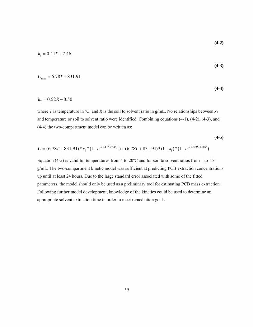
59

(4-2)

1 0.41 7.46k T= +

(4-3)

max 6.78 831.91C T= +

(4-4)

2 0.52 0.50k R= −

where T is temperature in ºC, and R is the soil to solvent ratio in g/mL. No relationships between x1

and temperature or soil to solvent ratio were identified. Combining equations (4-1), (4-2), (4-3), and

(4-4) the two-compartment model can be written as:

(4-5)

(0.41 7.46) (0.52 0.50)1 1(6.78 831.91)* *(1 ) (6.78 831.91)*(1 )*(1 )T t R tC T x e T x e− + − −= + − + + − −

Equation (4-5) is valid for temperatures from 4 to 20ºC and for soil to solvent ratios from 1 to 1.3

g/mL. The two-compartment kinetic model was sufficient at predicting PCB extraction concentrations

up until at least 24 hours. Due to the large standard error associated with some of the fitted

parameters, the model should only be used as a preliminary tool for estimating PCB mass extraction.

Following further model development, knowledge of the kinetics could be used to determine an

appropriate solvent extraction time in order to meet remediation goals.

60

Table 4.1. Comparison between PCB mass in controls and sum of PCB mass experimentally

extracted and PCB mass remaining in soil following experimental extraction.

Experimental Solvent Temperature

(ºC)

PCB mass in controls

(mg)

PCB mass in decanted solvent +

PCB mass in soil (mg)

Isopropyl Alcohol (IPA) 20 10.22 ± 0.14 14.69 ± 0.62

4 10.82 ± 0.04 19.23 ± 1.75

Ethanol (Eth) 20 3.45 ± 0.03 12.36 ± 3.88

4 8.73 ± 0.02 15.81 ± 1.23

Isooctane (Iso)* 20 16.87 ± 0.76 35.43 ± 4.79

Triethylamine (Tri) 20 8.45 ± 0.45 12.76 ± 0.68

Eth or IPA with Iso or Tri 20 6.22 ± 0.73 11.11 ± 1.21

4 6.69 ± 0.31 10.64 ± 1.29

* No DCB correction applied.

± Standard deviation.

61

Table 4.2. Results from solvent extractions with polar solvents.

Moisture Content of Optimal Extraction (% wt)

Temperature

(ºC)

Matrix With DCB

Correction

Statistically

Significant From

No DCB

Corrections

Statistically

Significant From

Isopropyl Alcohol

20 Decant 5% None 5% All but 10%

20 Soil 20% 0% and 5% 20% 5%

Ethanol

20 Decant 5% All but 0% 15% All

20 Soil 20% All but 15% 0% 10%

Isopropyl Alcohol

4 Decant 15% All but 20% 15% All but 20%

4 Soil 20% 5% and 15% 5%

10%

0% and 20%

None

Ethanol

4 Decant 5% All but 0% 5% All but 0%

4 Soil 0% All 0% All

62

Table 4.3. Results from solvent extraction with non-polar solvents at 20ºC.

Moisture Content of Optimal Extraction (% wt)

Matrix With DCB

Correction

Statistically

Significant From

No DCB

Corrections

Statistically

Significant From

Triethylamine

Decant 20% All but 15% 20% All

Soil 20% All 20% All

Isooctane

Decant 0%

20%

5%, 10%

All but 0%

Soil 0% All

63

Table 4.4. ANOVA Table for decanted solvent data treated as 24 Factorial Experiment.

Sum of

Squares

Degrees of

Freedom

Mean

Squared

Fobs

Main Effects

Moisture Content (%) 1643 1 1643 1.9

Polar Solvent 6380 1 6380 7.3 Significant

Non-Polar Solvent 149388 1 149388 170.9 Significant

Temperature 16678 1 16678 19.1 Significant

Interactions

Non-Polar * Temp 1103 1 1103 1.3

Polar * Temp 43 1 43 0.1

Polar * Non-Polar 34573 1 34573 39.6 Significant

Polar * Non-Polar * Temp 821 1 821 0.9

% * Temp 1340 1 1340 1.5

% * Non-Polar 810 1 810 0.9

% * Non-Polar * Temp 109 1 109 0.1

% * Polar 49130 1 49130 56.2 Significant

% * Polar * Temp 165 1 165 0.2

% * Polar * Non-Polar 2100 1 2100 2.4

% * Polar * Non-Polar*

Temp 474 1 474 0.5

Error 27967 32 874

Total 1.804E7 48

Corrected Total 292727 47

Factors with F> F1,32,0.05 = 4.2 were considered significant

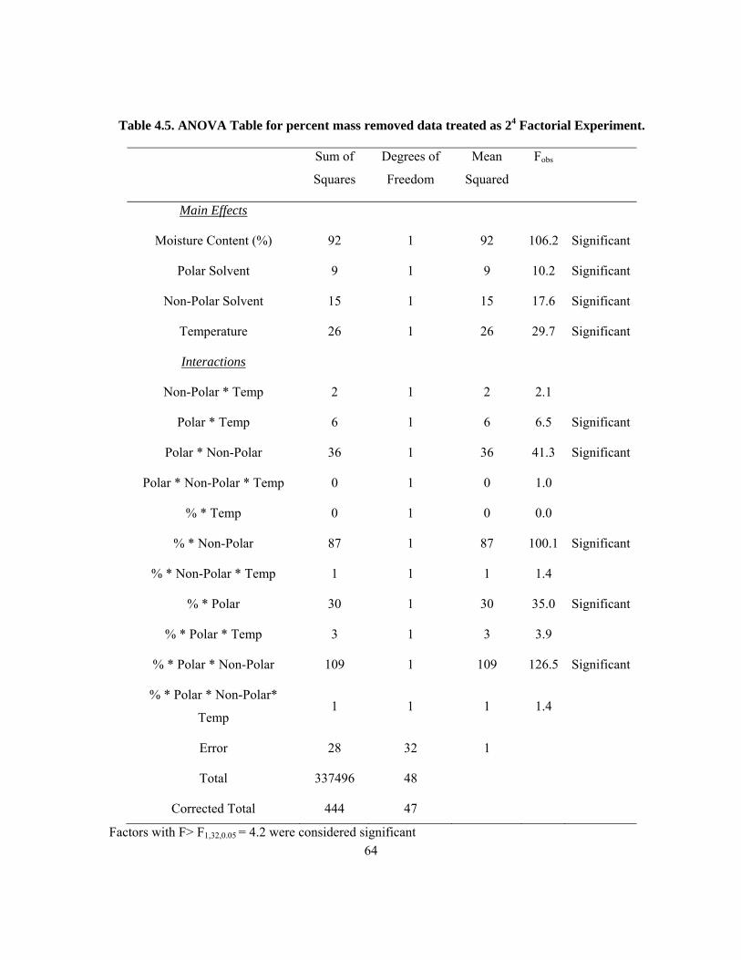
64

Table 4.5. ANOVA Table for percent mass removed data treated as 24 Factorial Experiment.

Sum of

Squares

Degrees of

Freedom

Mean

Squared

Fobs

Main Effects

Moisture Content (%) 92 1 92 106.2 Significant

Polar Solvent 9 1 9 10.2 Significant

Non-Polar Solvent 15 1 15 17.6 Significant

Temperature 26 1 26 29.7 Significant

Interactions

Non-Polar * Temp 2 1 2 2.1

Polar * Temp 6 1 6 6.5 Significant

Polar * Non-Polar 36 1 36 41.3 Significant

Polar * Non-Polar * Temp 0 1 0 1.0

% * Temp 0 1 0 0.0

% * Non-Polar 87 1 87 100.1 Significant

% * Non-Polar * Temp 1 1 1 1.4

% * Polar 30 1 30 35.0 Significant

% * Polar * Temp 3 1 3 3.9

% * Polar * Non-Polar 109 1 109 126.5 Significant

% * Polar * Non-Polar*

Temp 1 1 1 1.4

Error 28 32 1

Total 337496 48

Corrected Total 444 47

Factors with F> F1,32,0.05 = 4.2 were considered significant

65

Table 4.6. Grain Size range where highest PCB mass resides.

Grain size range of highest PCB mass (mm)

Soil ID With DCB

Correction

Statistically

Significant From

No DCB

Corrections

Statistically

Significant From

Dixie0707 2-19.05 All 2-19.05 All

Dixie0208 <0.425 >4.75 0.85-2.0 All but 0.425-0.85

Dixie0208-repeat* 0.85-2.0 All but 2.0-4.75 0.85-2.0 >4.75

* Excluded <0.425 mm grain sizes

66

Table 4.7 Kinetic Experiment Results

Two-Compartment

Model Parameters

Experiment 1

20ºC, 1g:1mL

Experiment 2

20ºC, 1g:0.75 mL

Experiment 3

4ºC, 1g:1mL

k1 - Fast compartment

extraction rate constant

(1/hour)

15.56 15.59 9.08

k2 – Slow compartment

extraction rate constant

(1/hour)

0.003 0.192 0.033

Cmax - Maximum

extractable PCB

concentration (µg/g)

967.6 967.6 859.0

x 1 –Fraction of mass in

the fast compartment

0.69 0.91 0.88

sy*- Standard deviation 41.0 30.7 16.1

*

2

1( )

m

i ii

y

y fs

m n=

−=

−

∑

where yi is the observed value, fi is the predicted value, m is the number of data points, and n is the number of parameters fit (Baird, 1962; Bendat and Piersol, 1971).

67

Figure 4.1. (a) PCB concentration removed using isopropyl alcohol at 20ºC, (b) PCB

concentration remaining in soil having undergone experimental extraction with isopropyl

alcohol at 20ºC, (c) PCB concentration extracted using isopropyl alcohol at 20ºC - repeat, (d)

PCB concentration extracted using isopropyl alcohol at 4ºC, (e) PCB concentration remaining

in soil having undergone experimental extraction with isopropyl alcohol at 4ºC

0

200

400

600

800

0 5 10 15 20

Extra

cted

Con

cent

ratio

n (u

g/g)

Moisture Content (% wt)

(a)0

100

200

300

400

0 5 10 15 20

Soil

Con

cent

ratio

n (u

g/g)

Moisture Content (% wt)

(b)

050

100150200250300350

0 5 10 15 20

Extra

cted

Con

cent

ratio

n (u

g/g)

Moisture Content (% wt)

(c)0

200400600800

10001200

0 5 10 15 20

Extra

cted

Con

cent

ratio

n (u

g/g)

Moisture Content (% wt)

(d)

0

100

200

300

400

0 5 10 15 20

Soil

Con

cent

ratio

n (u

g/g)

Moisture Content (% wt)

(e)

68

Figure 4.2. PCB concentration removed using ethanol at 20ºC (a) with DCB recovery

corrections and (b) without DCB recovery corrections, PCB concentration in soil having

undergone experimental extraction with ethanol at 20ºC (c) with DCB recovery corrections and

(d) without DCB recovery corrections, (e) PCB concentration removed from dry soil using

Ethanol at 4ºC, (f) PCB concentration remaining in dry soil after extraction with ethanol at 4ºC

0200400600800

1000

0 5 10 15 20

Extra

cted

C

once

ntra

tion

(ug/

g)

Moisture Content (% wt)

(a)0

200400600800

1000

0 5 10 15 20

Extra

cted

Con

cent

ratio

n (u

g/g)

Moisture Content (% wt)

(b)

0100200300400500

0 5 10 15 20

Soil

Con

cent

ratio

n (u

g/g)

Moisture Content (% wt)

(c)0

50100150200250

0 5 10 15 20

Soil

Con

cent

ratio

n (u

g/g)

Moisture Content (% wt)

(d)

0200400600800

1000

0 5 10 15 20

Extra

cted

Con

cent

ratio

n (u

g/g)

Moisture Content (% wt)

(e)0

50100150200250

0 5 10 15 20

Soil

Con

cent

ratio

n (u

g/g)

Moisture Content (% wt)

(f)

(a)

(c)

Figur

PCB

Mas

s Ext

ract

ed (%

)

(a)

Figure 4.3. P

re 4.4. Reacto

0

20

40

60

80

100(

)

M

0

0%

Percent mass

ors following

(d) 4ºC

Moisture Con

5 10 15

5%

s extracted a

g isopropyl a

- 0% and 5%

ntent (% wt)

5 20

10%

69

at 20ºC with (

lcohol extrac

% moisture c

PCB

Mas

s Ext

ract

ed (%

)

(b)

15%

(a) isopropyl

(

ction at (a) 2

ontent reacto

0

20

40

60

80

100

M

0

20%

l alcohol and

(b)

(d)

0ºC, (b) 20ºC

ors only

Moisture Cont

5 10 15

d (b) ethanol

C –repeat, (c)

tent (% wt)

20

) 4ºC,

70

(a) (b)

Figure 4.5. Ethanol following extraction at (a) 20ºC –decanted ethanol, (b) 4ºC - reactors

Figure 4.6. Mean PCB mass removed at 4ºC using (a) isopropyl alcohol and (b) ethanol

0

20

40

60

80

100

PCB

Mas

s Ext

ract

ed (%

)

Moisture Content (% wt)

(a) 0 5 10 15 20

0

20

40

60

80

100PC

B M

ass

Extra

cted

(%)

Moisture Content (% wt)

(b) 0 5 10 15 20

0% 5% 10% 15% 20% 0% 5% 10% 15% 20%

Ethanol

71

Figure 4.7. PCB concentration extracted at 20ºC with (a) isooctane and (b) triethylamine, PCB

concentration remaining in soil after extraction at 20ºC with (c) isooctane and (d) triethylamine

Figure 4.8. Mean PCB mass removed at 20 ºC using (a) isooctane and (b) triethylamine

0500

1000150020002500

0 5 10 15 20

Extra

cted

Con

cent

ratio

n (u

g/g)

Moisture Content (% wt)

(a)

Isooctane

0200400600800

1000

0 5 10 15 20

Extra

cted

Con

cent

ratio

n (u

g/g)

Moisture Content (% wt)

(b)

Triethylamine

0200400600800

1000

0 5 10 15 20

Soil

Con

cent

ratio

n (u

g/g)

Moisture Content (% wt)

(c)0

50

100

150

200

0 5 10 15 20

Soil

Con

cent

ratio

n (u

g/g)

Moisture Content (% wt)

(d)

0

20

40

60

80

100

PCB

Mas

s Ext

ract

ed (%

)

Moisture Content (% wt)

(a) 0 5 10 15 20

0

20

40

60

80

100

PCB

Mas

s Ext

ract

ed (%

)

Moisture Content (% wt)

(b) 0 5 10 15 20

72

(a)

(b)

Figure 4.9. Reactors after experimental extraction at 20ºC with (a) isooctane and (b)

triethylamine

0% 5% 10% 15% 20%

0% 5% 10% 15% 20%

73

Figure 4.10. PCB concentration extracted with decanted solvent data at (a) 20ºC and (b) 4ºC.

PCB concentration remaining in soil following extractions at (c) 20ºC and (d) 4ºC.

0

200

400

600

800Ex

tract

edC

once

ntra

tion

(ug/

g)

Solvent Combination

(a)EthTri5 EthTri20 IPATri5 IPATri20

EthIso5 EthIso20 IPAIso5 IPAIso20

20ºC

0

200

400

600

800

Extra

cted

Con

cent

ratio

n (u

g/g)

Solvent Combination

(b)EthTri5 EthTri20 IPATri5 IAPTri20

EthIso5 EthIso20 IPAIso5 IPAIso20

4ºC

0

50

100

150

200

Soil

Con

cent

ratio

n (u

g/g)

Solvent Combination

(c)EthTri5 EthTri20 IPATri5 IPATri20

EthIso5 EthIso20 IPAIso5 IPAIso20

20ºC

0

50

100

150

200

Soil

Con

cent

ratio

n (u

g/g)

Solvent Combination

(d)EthTri5 EthTri20 IPATri5 IPATri20

EthIso5 EthIso20 IPAIso5 IPAIso20

4ºC

74

Figure 4.11. Percent PCB mass extracted using sum of soil and solvent data at (a) 20ºC and (b)

4ºC

0

20

40

60

80

100

PCB

Mas

s Ext

ract

ed (%

)

Solvent Combination

(a)

EthTri5 EthTri20 IPATri5 IPATri20

EthIso5 EthIso20 IPAIso5 IPAIso20

20ºC

0

20

40

60

80

100

PCB

Mas

s Ext

ract

ed (%

)

Solvent Combination

(b)

EthTri5 EthTri20 IPATri5 IPATri20

EthIso5 EthIso20 IPAIso5 IPAIso20

4ºC

75

Figure 4.12. PCB concentration distribution by grain size for (a) Dixie0707, (b) Dixie0208, (c)

Dixie0208 – without DCB recovery corrections, (d) Dixie0208 - repeat

0

10

20

30

40

Soil

Con

cent

ratio

n (u

g/g)

(a)

0.07-0.25mm 0.25-2 mm2-19 mm >19 mm

0200400600800

1000120014001600

Soil

Con

cent

ratio

n (u

g/g)

(b)

<0.425 0.425 - 0.85 mm0.85 - 2.0 mm 2.0 - 4.75 mm> 4.75 mm

0200400600800

1000120014001600

Soil

Con

cent

ratio

n (u

g/g)

(c)

<0.425 0.425 - 0.85 mm

0.85 - 2.0 mm 2.0 - 4.75 mm

> 4.75 mm

0200

400600

8001000

12001400

1600So

ilC

once

ntra

tion

(ug/

g)(d)

0.43 - 0.85 mm 0.85 - 2 mm

2 - 4.75 mm >4.75 mm

(a)

F

F

Org

anic

Con

tent

(%w

/w)

(a)

Figure 4.13.

Figure 4.14. P

Figure 4.15.

0.0

0.5

1.0

1.5

2.0

2.5

3.0

3.5

Org

anic

Con

tent

(% w

/w)

<0.425 mm

0.85 - 2 m

>4.75 mm

0

Solvent follo

PCB contami

(a) Percent o

fractional o

m 0.42

mm 2-4.

m

0.07 – 0.25 mm

owing PCB e

inated soil so

organic conte

rganic carbo

25 - 0.85 mm

.75 mm

0.25 – 2.0mm

76

extraction fro

(b)

orted by grai

ent by weigh

on by weight

Frac

tiona

l Org

anic

Car

bon

(% w

/w)

(b)

00 2

om grain size

in size (a) Dix

ht for differen

for different

0.0

0.5

1.0

1.5

2.0

2.5

3.0

3.5

<0.425

0.85 - 2

> 4.75

2.00 – 19 mm

e groupingsw

xie0208 and

nt grain sizes

t grain sizes

5 mm 0

2.0 mm 2

mm

>19 mm

with ASE200

(b) Dixie070

s, (b) Percent

0.425 - 0.85 m

2.0 - 4.75 mm

7

t

mm

m

77

Figure 4.16. PCB extraction over time using a (a) 1g:1mL soil to solvent ratio at 20ºC, (b)

1g:0.75mL soil to solvent ratio at 20ºC, and (c) 1g:1mL soil to solvent ratio at 4ºC

0

200

400

600

800

1000

0 12 24 36 48

Extra

cted

PC

B C

once

ntra

tion

(ug/

g)

Time (hours)

(a)

Two Compartment Model

20ºC, 1 g soil: 1 mL solvent

0

200

400

600

800

1000

0 4 8 12 16 20 24

Extra

cted

PC

B C

once

ntra

tion

(ug/

g)

Time (hours)

(b)

Two Compartment Model

20ºC, 1 g soil: 0.75 mL solvent

0

200

400

600

800

1000

0 4 8 12 16 20 24Extra

cted

PC

B C

once

ntra

tion

(ug/

g)

Time (hours)

(c)

Two Compartment Model

4ºC, 1 g soil: 1 mL solvent

78

Chapter 5 Conclusions and Recommendations

5.1 Conclusions

Isopropyl alcohol, ethanol, triethylamine and isooctane were identified as promising solvents for PCB

extraction based on a literature review. The bench-scale experiments identified an interaction

between moisture content (5% versus 20%) and choice of polar solvent (isopropyl alcohol versus

ethanol) which influences solvent extraction efficiency. The solvent extractions conducted at 4ºC

showed that isopropyl alcohol performed better at higher moisture contents (15-20%) rather than at

the lower ones, and ethanol performed better at the lower moisture content (0-5%) as opposed to the

higher ones. There was a lack of statistically significant data to draw conclusions about the polar

solvents at 20ºC. The impact of elevated moisture content on solvent extraction efficiency could not

be quantified due to unreliable DCB spike recovery values.

The choice of non-polar solvent (triethylamine versus isooctane) was identified as significant.

Triethylamine achieved higher PCB extractions than the non-polar solvent isooctane. Triethylamine

was capable of achieving high PCB extraction efficiencies at both low and high moisture contents;

however, the best solvent extractions occurred at higher soil moisture contents (15-20%).

Combinations of solvents were also tested, but triethylamine alone performed best rather than in

combination with a polar solvent. While a polar solvent could be selected for a given soil moisture

content and temperature to achieve optimal extraction, it seems simplest that triethylamine be used

and that water is added to elevate the moisture content if it is not already high.

Temperature was determined to be significant in the mass of PCBs extracted. However no significant

interactions were determined between soil moisture content and temperature.

PCB mass was not evenly distributed amongst all grain sizes, and sorting PCB contaminated soil into

grain sizes may be an efficient way to target PCB contamination. It may allow for the exclusion of

less contaminated or uncontaminated soil that may otherwise be targeted, and reduce operation time

and expenses. More work is needed to establish a simple relationship between soil organic carbon and

PCB concentration.

79

The two-box release model proposed by Karickhoff (1980) fit PCB solvent extraction data for three

data sets for up to at least 24 hours of extraction. The two-compartment kinetic model was written in

terms of temperature and soil to solvent ratio to reflect the dependence of some of the model

parameters on these factors. This equation is valid for the Dixie0208 soil at temperatures ranging

from 4ºC to 20ºC, and a soil to solvent ratio from 1 to 1.3 g/mL. The model can be used to estimate

ideal solvent extraction conditions to meet remediation goals. The research conducted has improved

the understanding of solvent extraction so that PCB solvent extraction can be optimized in various

climates and under different conditions.

5.2 Recommendations

In future studies, it is recommended that PCBs be analyzed as congeners as opposed to Aroclors. This

change will eliminate the uncertainty caused by analyzing weathered samples that differ from Aroclor

standards and provide a more accurate picture of PCB extraction efficiency. Additional attempts

should be made to determine where the PCB mass is being lost during the analysis procedure in order

to improve DCB spike recovery and to improve PCB recovery consistency between samples. This

would likely eliminate contradicting results depending on whether or not DCB recovery is applied.

Further investigations are needed to determine the cause of the mass balance errors discussed in

section 4.1. Focus should be directed to how the soil is being handled and analyzed for remaining

PCBs.

It is recommended that triethylamine be used in the field as it outperformed isooctane and is optimal

at higher moisture contents. Water should be added to the soil to raise the moisture content to 15-20%

by weight to achieve optimal extraction. Further studies should be made into the effect of temperature

on solvent extraction using triethylamine.

A number of experiments had large variability between replicates and could be repeated. These

include the extractions using polar solvents at 20ºC. Repeating the organic carbon analysis on larger

sample sizes should reduce the variability between replicates and refine the relationship between PCB

mass and organic carbon amongst grain sizes. Finally, these studies should be repeated on other

contaminated soils to assess applicability to other sites and soil types.

Additional studies should be conducted to further develop the kinetic model and other factors known

to influence extraction should be considered. Data should be collected at earlier times (>0.5 hours) in

order to refine the fast extraction rate.

80

Bibliography

2008. Canadian Environmental Protection Act, SOR/2008-273, pp. 2078-2140. Ackerman, D.G. et al., 1983. Destruction and Disposal of PCBs by Thermal and Non-Thermal

Methods. Pollution Technology Review, 97. Noyes Data Corporation, New Jersey. Agarwal, S., Al-Abed, S.R. and Dionysiou, D.D., 2007. In Situ Technologies for Reclamation of

PCB-Contaminated Sediments: Current Challenges and Research Thrust Areas. Journal of Environmental Engineering, 133(12): 1075-1078.

Allen-King, R.M., Grathwohl, P. and Ball, W.P., 2002. New modeling paradigms for the sorption of hydrophobic organic chemicals to heterogeneous carbonaceous matter in soils, sediments, and rocks. Advances in Water Resources, 25: 985-1016.

Anderson, W.C. (Editor), 1995. Solvent/ Chemical Extraction. Innovative Site Remediation Technology, 3. WASTECH.

ASTM International, 2007. D 2974 - 07a: Standard Test Methods for Moisture, Ash, and Organic Matter of Peat and Other Organic Soils, West Conshohocken.

Baird, D.C., 1962. Chapter 6: Experiment Evaluation, Experimentation: An Introduction to Measurement Theory and Experiment Design. Prentice-Hall, Inc., Englewood Cliffs, New Jersey.

Bendat, J.S. and Piersol, A.G., 1971. Chapter 4: Review of Statistical Principles, Random Data: Analysis and Measurement Procedures. Wiley-Interscience, New York.

Calabrese, E.J., Kostecki, P.T. and Dragun, J. (Editors), 2006. Successes and Challenges. Contaminated Soils, Sediments and Water, 10. Springer, New York.

Carroll, K.M., Harkness, M.R., Bracco, A.A. and Balcarcel, R.R., 1994. Application of a Permeant/Polymer Diffusional Model to the Desorption of Polychlorinated Biphenyls from Hudson River Sediments. Environmental Science and Technology, 28(2): 253-258.

Cassidy, D. and Hampton, D., 2009. The Effect of Persulfate Oxidation of PCBs in River Sediments on Sulfate-Reducing Bacteria (SRB), Fifth International Conference on Remediation of Contaminated Sediments. Battelle, Jacksonville, Florida.

Churcher, P.L. and Dickhout, R.D., 1987. Analysis of Ancient Sediments for Total Organic Carbone - Some New Ideas. Journal of Geochemical Exploration, 29: 235-246.

Craig, R.F., 2002. Soil Mechanics. Spon Press, New York. Crine, J.-P. (Editor), 1988. Hazards, Decontamination, and Replacement of PCB: A Comprehensive

Guide. Environmental Science Research, 37. Plenum Press, New York. Dhol, A.S., 2005. An Investigation of a Photochemical Approach for the Remediation of PCB-

Contaminated Soils, University of Calgary, Calgary, 260 pp. Donnelly, J.R. et al., 1996. Modular Methodology for Determination of Polychlorinated Biphenyls in

Soil as Aroclors and Individual Congeners. Journal of AOAC International, 79(4): 953-961. EPA, 1994. Method 3541: Automated Soxhlet Extraction. EPA, 1996a. Method 3540C: Soxhlet Extraction. EPA, 1996b. Method 3665A: Sulfuric Acid/ Permanganate Cleanup. EPA, 1996c. Method 8000B: Determinative Chromatographic Separations. EPA, 1996d. Method 8082: Polychlorinated Biphenyls (PCBs) by Gas Chromatography. EPA, 2000a. Method 3545A: Pressurized Fluid Extraction (PFE). EPA, 2000b. Method 3620C: Florisil Cleaup. EPA, 2007a. Method 3500C: Organic Extraction and Sample Preparation. EPA, 2007b. Method 3550C: Ultrasonic Extraction. Erickson, M.D., 1993. Remediation of PCB Spills. Lewis Publishers, U.S.A.

81

Fang, Y. and Al-Abed, S.R., 2007. Partitioning, Desorption, and Dechlorination of a PCB Congener in Sediment Slurry Supernatants. Environmental Science and Technology, 41(17): 6253-6258.

Forsey, S., 2007. Organic Chemistry Lecturer, Chemistry Department, University of Waterloo, Waterloo, pp. Conversation.

Fox, T.G. and Flory, P.J., 1954. The Glass Temperature and Related Properties of Polystyrene. Influence of Molecular Weight. Journal of Polymer Science, 14: 315-319.

Gripton, C., 2007. Maxxam Analytics, pp. Phone Call. Hawker, D.W. and Connell, D.W., 1988. Octonol-Water Partition Coefficients of Polychlorinated

Biphenyl Congeners. Environmental Science and Technology, 22(4): 382-387. Huang, W., Peng, P.a., Yu, Z. and Fu, J., 2003. Effects of organic matter heterogeneity on sorption

and desorption of organic contaminants by soils and sediments. Applied Geochemistry, 18: 955-972.

Hurst, R.W. (Editor), 1987. Practical Solutions to PCB Problems. Industry and PCBs, 1. The Canadian Electricity Forum Inc., Pickering.

Hutzinger, O., Safe, S. and Zitko, V., 1974. The Chemistry of PCB's. CRC Press, Cleveland. Jakher, A., Achari, G. and Langford, C.H., 2007. An Investigation Into Solvent Extraction of PCBs

From Weathered Soils. Environmental Technology, 28(1): 49-57. Johnson, R.A., 2000. Chapter 13: Factorial Experimentation, Miller & Freund's Probability and

Statistics for Engineers. Prentice Hall, Upper Saddle River, NJ. Kadla, J.F., Kubo, S., Gilbert, R.D. and Venditti, R.A., 2002. Lignin-based Carbon Fibers. In: T.Q.

Hu (Editor), Chemical Modification, Properties, and Usage of Lignin. Kluwer Academic/ Plenum Publishers, New York, pp. 121-139.

Karickhoff, S.W., 1980. Sorption Kinetics of Hydrophobic Pollutants in Natural Sediments. In: R.A. Baker (Editor), Contaminants and Sediments. Ann Arbor Science, Michigan, pp. 193-205.

Kennedy, J.B. and Neville, A.M., 1976. Chapter 11: Rejection of Outliers, Basic Statistical Methods for Engineers & Scientists. Harper & Row, Publishers, New York.

Korte, N.E. et al., 2002. The effect of solvent concentration on the use of palladized-iron for the step-wise dechlorination of polychlorinated biphenyls in soil extracts. Waste Management, 22: 343-349.

Lamoureux, E.M. and Brownawell, B.J., 1999. Chemical and Biological Availability of Sediment-Sorbed Hydrophobic Organic Contaminants. Environmental Toxicology and Chemistry, 18(8): 1733-1741.

Lassere, J.-P. et al., 2008. Effects of the endocrine disrupting compounds atrazine and PCB 153 on the protein expression of MCF-7 human breast cancer cells. Toxicology Letters, 180: S122.

Lide, D.R. (Editor), 1998. CRC Handbook of Chemistry and Physics (1998-1999). CRC Press. Lou, J., Paravastu, A.K., Laibinis, P.E. and Hatton, T.A., 1997. Effect of Temperature on the

Dielectric Relaxation in Solvent Mixtures at Microwave Frequencies. Journal of Physical Chemistry A, 101(51): 9892-9899.

Lucht, L.M., Larson, J.M. and Peppas, N.A., 1987. Macromolecular Structure of Coals. 9. Molecular Structure and Glass Transition Temperature. Energy & Fuels, 1(1): 56-58.

Mackay, D., 2006. Handbook of Physical-Chemical Properties and Environmental Fate for Organic Chemicals. CRC Press, 919 pp.

Meckes, M.C., Renard, E., Rawe, J. and Wahl, G., 1992. Solvent Extraction Processes: A Survey of Systems in the SITE Program. Journal of Air Waste Management Association, 42(8): 1118-1121.

82

Meckes, M.C., Tillman, J., Drees, L. and Saylor, E., 1997. Removal of PCBs from a Contaminated Soil Using CF-Sytems Solvent Extraction Process. Journal of Air Waste Management Association, 47: 1119-1124.

Meckes, M.C., Wagner, T.J., Tillman, J. and Krietemeyer, S., 1993. SITE Demonstration of the Basic Extractive Sludge Treatment Process. Journal of Air Waste Management Association, 43(9).

National Research Council, 2001. A risk-management strategy for PCB-contaminated sediments. National Academy Press.

Ontario Government, 1990a. R.R.O. 1990, Regulation 352 - Mobile PCB Destruction Facilities. Ontario Government, 1990b. R.R.O. 1990, Regulation 362 - Waste Management - PCB's. Ontario Ministry of the Environment, 2000. Protocol for Sampling and Testing at PCB Storage Sites

in Ontario. In: S.D. Branch (Editor). Queen's Printer for Ontario. Ontario Ministry of the Environment, 2004. Soil, Ground Water and Sediment Standards for Use

Under Part XV.1 of the Environmental Protection Act. Queen's Printer for Ontario. Ontario Ministry of the Environment, 2006. The Determination of Polychlorinated Biphenyls (PCBs),

Organochlorines (OCs) and Chlorobenzenes (CBs) in Soil and Sediments by Gas Liquid Chromatography-Electron Capture Detection (GLC-ECD). In: Q.M.U. Laboratory Services Branch (Editor).

Ontario Ministry of the Environment, 2007. Soil, Ground Water and Sediment Standards for Use Under Part XV.1 of the Environmental Protection Act.

Perkins, C., 2008. Conversation, Waterloo. Pignatello, J.J. et al., 2006. Nonlinear and Competitive Sorption of Apolar Compounds in Black

Carbon-Free Natural Organic Materials. Journal of Environmental Quality, 35: 1049-1059. Schaumann, G.E. and LeBoeuf, E.J., 2005. Glass Transitions in Peat: Their Relevance and the Impact

of Water. Environmental Science and Technology, 39(3): 800-806. Smith, K.E., Schwab, A.P. and Banks, M.K., 2007. Phytoremediation of Polychlorinated Biphenyl

(PCB) - Contaminated Sediment: A Greenhouse Feasibility Study. Journal of Environmental Quality, 36: 239-244.

Sonic Environmental Solutions Inc., 2007. Sonic POP Treatment Facilities. Stevenson, F.J., 1982. Humus Chemistry: Genesis, Composition, Reactions. John Wiley & Sons,

Toronto. Strachan, W.M.J., 1988. Polychlorinated Biphenyls (PCBs) - Fate and Effects in the Canadian

Environment. In: C.a. Protection (Editor). Environment Canada. Streitwieser, A., Heathcock, C.H. and Kosower, E.M., 1992. Introduction to Organic Chemistry.

Maxwell MacMillan Canada, Toronto. Teuten, E.L., Rowland, S.J., Galloway, T.S. and Thompson, R.C., 2007. Potential for Plastics to

Transport Hydrophobic Contaminants. Environmental Science and Technology, 41(22): 7759-7764.

Tisa, K.N., 2007. Re: PCB analysis, Boston, pp. Email. Trowbridge, T.D. and Holcombe, T.C., 1996. The Carver-Greenfield Process: Dehydration / Solvent

Extraction Technology for Waste Treatment. Environmental Progress, 15(3): 213-220. United Nations Environment Programme, Stockholm Convention on Persistent Organic Pollutants. United Nations Environment Programme, 2008. Stockholm Convention on persistent organic

pollutants (POPs). Secretariat of the Stockhold. Valentin, M.M., 2000. Laboratory Study of Solvent Extraction of Polychlorinated Biphenyls in Soil,

McGill University, Montreal. Waid, J.S. (Editor), 1986. PCBs and the Environment, 1. CRC Press.

83

Waisner, S., Medina, V.F., Morrow, A.B. and Nestler, C.C., 2008. Evaluation of Chemical Treatments for a Mixed Contaminant Soil. Journal of Environmental Engineering, 134(9): 743-749.

Weber, W.J., LeBoeuf, E.J., Young, T.M. and Huang, W., 2001. Contaminant Interactions with Geosorbent Organic Matter: Insights Drawn from Polymer Sciences. Water Resources Research, 35(4): 853-868.

Wright, A.G. and Rosta, P.R., 1998. Dewatering System Is High and Dry. ENR, 240(13): 10-11. Wu, S.-c. and Gschwend, P.M., 1988. Numerical Modeling of Sorption Kinetics of Organic

Compounds to Soil and Sediment Particles. Water Resources Research, 24(8): 1373-1383. Xing, B. and Pignatello, J.J., 1997. Dual-Mode Sorption of Low-Polarity Compounds in Glassy

Poly(Vinyl Chloride) and Soil Organic Matter. Environmental Science and Technology, 31(3): 792-799.

Xing, B. and Pignatello, J.J., 1998. Competitive Sorption between 1,3-Dichlorobenzene or 2,4-Dichlorophenol and Natural Aromatic Acids in Soil Organic Matter. Environmental Science and Technology, 32(5): 614-619.

Xing, B., Pignatello, J.J. and Gigliotti, B., 1996. Competitive Sorption between Atrazine and Other Organic Compounds in Soils and Model Sorbents. Environmental Science and Technology, 30(8): 2432-2440.

Zhang, W.-x., 2003. Nanoscale iron particles for environmental remediation: An overview. Journal of Nanoparticle Research, 5: 323-332.

84

Appendix A Ranking Potential Solvents

Table A.1. Ranking scheme for potential polar solvents

Weight 0.2 0.05 0.3 0.05 0.4

Polar Solvent Influence of temperature on Viscosity

Polarity * Cost Recommendations Toxicity Score

Methanol 5 5 5 4 0 2.95

Ethanol 4 2.6 2.8 0 3 2.96

1-propanol 3 1.1 0.3 0 5 2.74

Isopropyl alcohol

2 0.9 3.9 5 4 3.46

1-butanol 1 0.2 0 0 2 1.11

2-butanol 0 0 1.7 0 1 0.8

* based on dielectric constants

Table A.2. Ranking scheme for potential non-polar solvents

Weight 0.15 0.3 0.15 0.4

Non-Polar Solvent

Influence of temperature on Viscosity

Polarity * Cost Toxicity Score

Isooctane 0 2 5 1.5 1.20

Triethylamine 2 1.8 2.8 0 1.13

Ethyl acetate 1 0 0.3 2 1.06

* based on dielectric constants