Optimizing Artificial Force Fields forAutonomous Drones in the Pylon

Challenge using Reinforcement Learning

Martijn F.W. van der Veen

Optimizing Artificial Force Fields forAutonomous Drones in the Pylon

Challenge using Reinforcement Learning

Martijn F.W. van der Veen5964008

Bachelor thesisCredits: 15 EC

Bacheloropleiding Kunstmatige Intelligentie

University of AmsterdamFaculty of ScienceScience Park 904

1098 XH Amsterdam

SupervisorDr. A. Visser

Intelligent Systems Lab AmsterdamFaculty of Science

University of AmsterdamRoom C3.237

Science Park 904NL 1098 XH Amsterdam

July 28th, 2010

Abstract

The idea of imaginary forces acting on a robot has gained a lot ofinterest from robotics researchers in the nineties as useful and easy-to-set-up paradigm for navigation without collisions. However, theforce field essentially is not optimal, leaving room for improvements.A common used method for learning optimal policies is ReinforcementLearning. This thesis tries to apply reinforcement learning to forcefields in a way to improve the initial force field. The framework isapplied, with some additional improvements, to the “Figure-Eight”task using an aerial robot. Some interesting results follow from the(simulated) experiments, and the possibility of the proposed frameworkwill be evaluated.

keywords:reinforcement learning, potential field methods, force fields, figure-eight,drones, imav2011

Contents

1 Introduction 21.1 Motivation . . . . . . . . . . . . . . . . . . . . . . . . . . . . 3

2 Related Work 32.1 Force Fields . . . . . . . . . . . . . . . . . . . . . . . . . . . . 32.2 Reinforcement Learning . . . . . . . . . . . . . . . . . . . . . 52.3 Combining Potential Fields and Reinforcement Learning . . . 7

3 Methodology 73.1 Artificial Force Fields . . . . . . . . . . . . . . . . . . . . . . 83.2 Reinforcement Learning . . . . . . . . . . . . . . . . . . . . . 93.3 Figure-Eight . . . . . . . . . . . . . . . . . . . . . . . . . . . . 11

4 Practical Tests 134.1 Simple Simulation . . . . . . . . . . . . . . . . . . . . . . . . 134.2 USARSim simulation . . . . . . . . . . . . . . . . . . . . . . . 134.3 IMAV2011 & AR.Drone . . . . . . . . . . . . . . . . . . . . . 14

5 Results 155.1 Simple Simulation . . . . . . . . . . . . . . . . . . . . . . . . 155.2 USARSim Simulation . . . . . . . . . . . . . . . . . . . . . . 18

6 Conclusion & Discussion 18

7 Future Research 20

1 Introduction

People seem to think that the goal of Artificial Intelligence is the creation ofautonomous, intelligent robots. One could state that, at least in the field ofrobotics, it seems indeed to be the ultimate goal. Although a lot of progresshas been made in the last couple of decades, the ultimate goal still appearsfar from reached. Different sub-problems ask for different algorithms, and‘the best’ framework does not (yet) exists. In the course of time, a lot ofalgorithms have been invented and are investigated exhaustively, and somebecame part of the standard toolbox1. Since there still are a lot of challenges,existing ideas are being shaped and new algorithms are being proposed, andtested on both existing and new problems.

One challenge within robotics is the simple task of autonomous navigatingtowards a goal, without hitting obstacles. One of the proposed methodsthat try to solve this task uses artificial forces to guide the robot [5]. Therobot is attracted by the goal, while obstacles spread a repelling force. Theapproach works, but does not give an optimal path. This leads to thequestion whether the forces, which look like a good starting point, could beimproved by learning.

A well-known approach within robotics for learning is reinforcement learn-ing. This semi-unsupervised learning methodology uses the intuitive notionof reward and punishment received from the environment to learn optimalactions for possible situations (i.e., locations within the environment). Theobjective of this thesis is to take the forces, or force field, as initial set up,and improve it using reinforcement learning. The improved force field shouldlead to better paths that cause the robot to move faster to the goal.

The proposed method will be tested in the often-used Figure-Eight (Pylon)challenge using an aerial robotics platform. The objective of the Figure-Eight challenge is to move in figure-eight’s around two poles. The tests willbe used to gain insight in the benefits and possibly disadvantages of theproposed method.

1As an example, the SLAM algorithm, for both mapping and localizing in unknownenvironments, is being used frequently; http://openslam.org

2

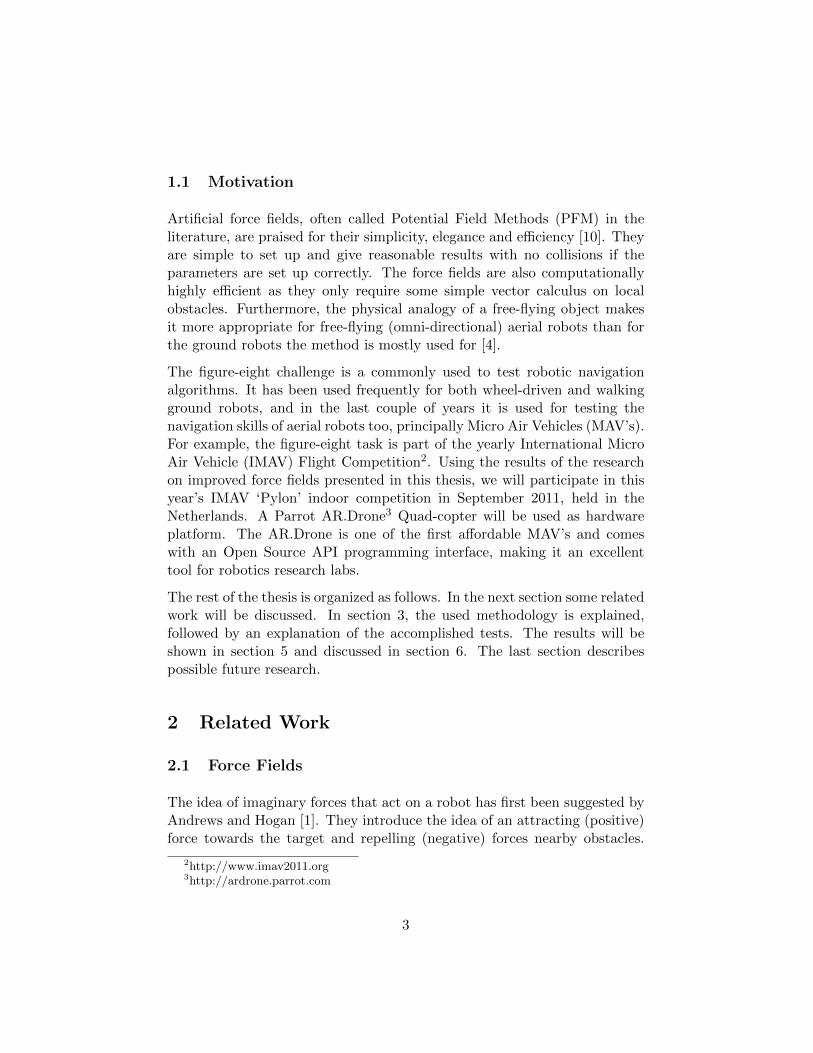
1.1 Motivation

Artificial force fields, often called Potential Field Methods (PFM) in theliterature, are praised for their simplicity, elegance and efficiency [10]. Theyare simple to set up and give reasonable results with no collisions if theparameters are set up correctly. The force fields are also computationallyhighly efficient as they only require some simple vector calculus on localobstacles. Furthermore, the physical analogy of a free-flying object makesit more appropriate for free-flying (omni-directional) aerial robots than forthe ground robots the method is mostly used for [4].

The figure-eight challenge is a commonly used to test robotic navigationalgorithms. It has been used frequently for both wheel-driven and walkingground robots, and in the last couple of years it is used for testing thenavigation skills of aerial robots too, principally Micro Air Vehicles (MAV’s).For example, the figure-eight task is part of the yearly International MicroAir Vehicle (IMAV) Flight Competition2. Using the results of the researchon improved force fields presented in this thesis, we will participate in thisyear’s IMAV ‘Pylon’ indoor competition in September 2011, held in theNetherlands. A Parrot AR.Drone3 Quad-copter will be used as hardwareplatform. The AR.Drone is one of the first affordable MAV’s and comeswith an Open Source API programming interface, making it an excellenttool for robotics research labs.

The rest of the thesis is organized as follows. In the next section some relatedwork will be discussed. In section 3, the used methodology is explained,followed by an explanation of the accomplished tests. The results will beshown in section 5 and discussed in section 6. The last section describespossible future research.

2 Related Work

2.1 Force Fields

The idea of imaginary forces that act on a robot has first been suggested byAndrews and Hogan [1]. They introduce the idea of an attracting (positive)force towards the target and repelling (negative) forces nearby obstacles.

2http://www.imav2011.org3http://ardrone.parrot.com

3

The target is viewed as a point which exerts a constant force towards himselfon all locations, while the obstacles exert a repelling force towards the robotinversely proportional to the distance between the obstacle and the robot.

The force field framework, later on called Potential Field Methods (PFM),was further investigated in the 90’s by many researchers in the robotics areaand became quite popular for a short time as obstacle avoidance method. Forexample, Koren and Borenstein [2] developed the Virtual Force Field (VFF)which will discretize the environment and uses a certainty grid to representthe certainty of finding an obstacle at each grid position. Obstacles can thusbe unknown initially, but it is assumed that the location of both the robotand the goal is known.

Two forces are being calculated in PFM: the attractive force ~Ft, and the totalrepelling force ~Fr. The resultant force vector is the sum of both: ~R = ~Ft+ ~Ft.The direction determines the robot’s steering-rate, which is a constant timesthe difference between the current and the desired direction. This is, ofcourse, based on the idea of wheel-based robots; omni-directional vehiclescould simply proceed their path in the desired direction. The new directionis thus determined by the strength (length of vector) of the repelling forcesrelative to the attracting force constant γ. Note that the length is notimportant and a constant speed is used.

The Virtual Force Field uses a Active Window of grid cells nearby to calcu-late the vectors ~Fr and ~Ft as:

~Fr =∑c

Fc =∑c

δ

dn(c, r)

(~Pc − ~Pr)

d(c, r)

and

~Ft = γ(~Pt − ~Pr)

d(t, r)

where c stands for a cell, r for the robot and t for the target, δ is a valuedetermined by a negative force constant, the certainty of an object beingat cell c and the size of the robot, γ a target force constant, ~P the variouspositions, and d(c, r) the distance between cell c and the robot. Thus, theattracting target force has constant size and points towards the target, andthe repelling force is the sum of all cells possibly containing an obstacle,inversely proportional to the distances to the robot. In practice, n is oftenchosen to be 2.

More extensions have been proposed, such as the Vector Field Histogramby Borenstein which calculates directions with a high concentration of free

4

space, Navigation Fields which are potential fields that do not have localminima but are difficult to create, methods incorporating global path plan-ning, and extensions to deal with motion dynamics at high speed movement[6]. This last extension uses a dynamic window approach where the size ofthe active window is changed according to current speed and direction, totake into account the inertia of both the rotation and the translation. Foromni-directional robots such as quad-copters, the rotational inertia is not aproblem, but the translation inertia could cause problems. However, whenlearning is involved, possibly wrong initial forces could be corrected. An-other extension is the use of a variable attracting force determined by thedistance, which could help avoiding the problem of local minima with canoriginate out of many obstacles near the goal [7].

The Potential Field Methods are reported to be successful in practice [3,10, 4], both in simulation and real-world application. Some limitations aredescribed too [10], which are discussed in section 6. Later on, more advancedmethods were developed that are more proficient for small environmentsthan Potential Field Methods, and the PFM became less used. For largeropen areas such as in the “Figure-Eight” task, PFM are still useful. Anyway,the most important objective of the proposed methods is avoiding obstacles,leaving room for more efficient paths. Hence, it is worth examining anadjustment of the potential field method.

2.2 Reinforcement Learning

A well-known method for learning and improving policies is ReinforcementLearning [12, p.51-82]. RL uses the intuitive idea of reward and punishment(or negative reward) that follow on actions of an agent. In learning methodsconcerning supervision, the best action possible will be told to the agent afteracting in a certain situation. In practical problems, the best action is oftennot known, but a certain value of the resulting state could be defined. In RLthe reward of different actions for different states is being used to updateeither the value function, that determines the potential value of each state,or the policy, that maps possible observed states to the best known actions.The reward function thus defines the goal of the task being accomplished,without specifying exactly how the task will be accomplished. The goal ofthe Reinforcement Learning problem is to maximize the expected (average)total reward over time, called return, so to maximize the following function

5

[9]:

limh→∞E(1

h

h∑t=0

rt)

or, more often cited [11], to find the optimal policy π∗:

π∗ = argmaxπ[E(∞∑t=0

γtrt)]

where rt is the immediate reward following the last action and determinedby the current state, and γ is some discount parameter to make the infinitesum finite. The interaction with the environment enables the agent to learnoptimal actions for each state by choosing the action that has the largestexpected return.

Updating the agent’s knowledge could be accomplished by using a methodinvolving some form of temporal difference (TD) [12, p.133-157], which up-dates the value function, or a more exotic method such as an evolutionaryalgorithm (EA) [11], which updates the policy directly. TD techniques up-date the values or value function parameters based on the direct reward andthe difference between the current and last potential state value, weightedwith a learning parameter:

V (st−1)← V (st−1) + α[rt + γV (st)− V (st−1)]

orV (st−1)← (1− α)V (st−1) + α(rt + γV (st))

with V () the value of a state, rt the current reward and α the learningparameter. The update is thus based on the difference of the value of the lastvisited state and the value of the current state, or a weighted combinationof the old expected (long-term) return value and the current one based oncurrent reward and the value of the next state. On the side of evolutionaryalgorithms, whole policies instead of values are being evaluated and ‘evolve’to better policies.

To use the knowledge learned from experience, as well as gather new knowl-edge, a trade-off between exploitation and exploration has to be made. Inpractice, often some percentage of the actions is chosen random and theremaining actions are determined by the value function or policy learned sofar.

6

2.3 Combining Potential Fields and Reinforcement Learning

The Potential Force Method basically is a gradient descent search methoddirected towards minimizing the potential function. The potential func-tion is defined by summing over the forces from goal to each point, with adescending slope towards the goal and hyperbolic hills around obstacles.

An interesting idea using the gradient descent view of the PFM is proposedin [11], which is the only paper known to us that claims to combine reinforce-ment learning and potential force fields. The potential field model as statedin the last paragraph shares some features with the reinforcement learningmodel. Using these similarities they redefined a maze problem, originallystated in a reinforcement learning model, as a potential field problem:

• States with positive rewards become attractive sources

• States with negative rewards become repulsive sources

• Other states have no attractive or repulsive force

Using these rules, they rewrite the RL problem, in fact creating a path plan-ning problem from a optimization problem. Applying the proposed transi-tion in [11], their maze problem consisting of a 25x28 state grid becomes agrid of objects exerting attracting or repelling forces, used for direct reward.With the utility function representing the map given, they learn a policy tonavigate through this map. The policy in their case consists of four discreteactions (North, West, South, East) for each grid point.

In this thesis a policy is learned with continuous actions; the drone can flyin any direction and the optimal policy will consist of the optimal direc-tions. The path planning problem is thus being optimized by reinforcementlearning. The proposed “Figure-Eight” task will use a big force field withomni-directional free-flight possibilities, instead of small corridors with dis-crete locations.

3 Methodology

The objective of this thesis is to start with an initial potential field, whichis best seen as a force field in this methodology. The initial force field setup, which is a reasonable point to start concerning navigation tasks, willbe followed by improvements of the force field using a method based on the

7

reinforcement learning method temporal difference. First will be explainedthe initial force field set up including necessary steps to prepare for thenext step, which is the learning cycle, where experience in the environmentcontaining the specified problem will make changes to the force field. Thenthis framework is viewed in context of the “Figure-Eight” problem, withsome additional comments on how to incorporate the problem with the forcefields.

3.1 Artificial Force Fields

Initial Force Field The Potential Field Method sets a force field fora particular problem. A robot navigating through the environment will‘perceive’ forces from different sources, resulting in a total force on eachlocation. To be able to learn a better force field a discretization step isapplied where for a set of discrete locations L the corresponding total forceis being calculated. The forces with their corresponding location are calledforce vectors and the set of force vectors L a discretized force field. Notethat this transition is done only once, meaning that dynamically movingobjects do not change the force vectors directly. However, reinforcementlearning makes room for dynamically changing environments. Nonetheless,the method will work best for static environments.

The discretization could be a uniform distributed field, or more elaboratedistributions such as coarse coding or a particle filter. With a particle filter,more particles could be set at locations often visited or with big differences inthe value function (i.e., narrow corridors). In our implementation, a uniformdistributed field is used.

Three force sources could contribute to the total force:

• Obstacles apply a force towards the locations inversely quadratic pro-portional with the distance, with a maximum range

• Target applies a force towards himself with constant strength for alllocations

• Bias to incorporate important aspects of a specific task, such as pre-ferred rotational direction around a particular object

All partially forces add together resulting in the force vectors. Appropriatesettings and possibly added bias forces are problem-specific and some tweak-ing could be needed, although the exact values do not seem that important

8

(see also section 5).

Speed update The force vector being used to update the speed is chosenby nearest neighbour. Since a unique vector is being used each time, it iseasier to update the visited vectors later on than it would have been with ainterpolation step.

Wheel-driven vehicles need some time to change the direction of movement.However, the focus lies on aerial drone vehicles (MAV’s), which have omni-directional fly capacities. The force vector could thus directly be applied tothe drone without the need for turn instructions. For low speed the newspeed will be almost identical to the force vector applied to the vehicle,while for high speed movements the inertia could play a role too and thenew speed (vector) has a small component of the last speed (vector) too.

In practice, drones often have a maximum speed, preventing the drone frommoving so fast that the force field has not enough power to steer the vehicle.Alternatively, an artificial maximum could be set. In addition it seems usefulto set a minimum speed, to prevent the drone from coming to a standstillin areas with small force vectors. When the minimum speed is set equal tothe maximum speed, the paths will be traversed with constant speed. Thisturns out to be a natural choice in big open areas, but will be less proficientin problems with small areas where less speed could be necessary.

If the parameters are set up correctly, the drone now moves towards the goalwithout hitting obstacles. An example task is shown in figure 1, which hasa left-rotation bias around one obstacle. Shown in yellow are the vectorsbeing selected by nearest neighbour during the run. As could be seen, thepath does lead to the goal but is not very efficient.

3.2 Reinforcement Learning

Exploration A parameter ε is set that determines the amount of explo-ration. During an exploration step, instead of the actual nearest force vectora random force vector is created and used until a next force vector is reached.

Value Update The return function r(~L) returns for the current location~L a positive value when a goal is reached, a negative value when hitting anobstacle and zero otherwise. To use the reward information for estimating

9

Figure 1: Potential Field, leading a drone towards a goal (simple simulation)

the expected long-term return, each vector is extended with a (potential)value V . This value is being used for the expected return value4, and isnecessary for temporal difference used by the vector update.

The value corresponding to the last force vector ~Ft−1 is updated each timea new force vector ~Ft is being used using TD:

V (~Fp−1)← V (~Fp−1) + α[r(~Lp) + γV (~Fp)− V (~Fp−1)]

orV (~Fp−1)← (1− α)V (~Fp−1) + α(r(~Fp) + γV (~Fp))

where ~Fp−1 stands for the last force vector being used (with p−1 the previous

force vector position) and ~Lp for the current location.

To increase the learning speed, the value update rule could be used back-wards for the h vectors in the history.

Vector Update The force vector will be updated as a weighted sum ofthe force vector and the speed vector that was actually flown5.

4see section 7 on future research for an alternative approach5If the inertia would become stronger on high speeds, one could calculate the force

vector that would be needed to fly the speed vector and use the result, instead of thespeed vector.

10

Paths that result in high returns were (obviously) better than paths thatresult in lower returns. Therefore speed vectors that increases the (potential)value V more should be weighted more than speed vectors that increase Vless. Paths resulting in a negative return get a negative difference value,which effectively points the weighted speed vector to the opposite direction.

The vector update follows:

~Fp−1 ← (1− λ)~Fp−1 + λ~Sp−1

where ~St−1 stands for the previous speed vector, and λ determined by α andthe temporal difference:

λ = α(V (~Fp)− V (~Fp−1))

It is important that the values do not exceed the boundaries -1 and 1 if thereis no maximum speed set, since otherwise the force vectors could increasetheir length to high values not only due to long speed vectors, but also dueto high TD and λ weights.

A history of the last H used force vectors could be remembered and used toupdate a couple of vectors back each time based on the temporal differencebetween the value of the current vector and the value of each vector h stepsback in history divided by the number of vectors h, setting lambda to:

λ = αV (~Fp)− V (~Fp−h)

h

Using this history update faster learning could be obtained with less episodesneeded for reasonable results.

3.3 Figure-Eight

The goal of the Figure-Eight task is to move in a Figure-Eight around twopoles (figure 2). The task occurs in a static environment and is essentiallya 2D problem, although the used method should work equally well in 3Dsince general vectors are being used in all formulas. We will discuss somedifficulties concerning the use of the framework we talked over until now,and show the steps being accomplished to define the “Figure-Eight” taskinto the framework.

11

Figure 2: Figure-Eight pylon challenge

Force Fields One difficulties in using a potential field for the “Figure-Eight” task is the continue characteristic of the latter, which makes defininga clear target location difficult. Another one is the center of the field (be-tween the two poles), which sometimes needs to be passed in one directionand other times in the other direction. Both difficulties are solved by intro-ducing two different stages, one for ‘left to right’ and one for ‘right to left’.Each stage has its own stage transition which is defined as passing the linethrough both poles at the outside of the corresponding pole (right or left).Each stage has its own force field too, enabling the robot to learn differentforces for the same locations, depending on the current location of the targetline.

Reinforcement Learning The reward function returns 1 for a state tran-sition and -1 for a collision. The reinforcement learning occurs within stagesand is restarted after a transition, as a result of which the values fall fromalmost 1 to possibly lower than 0 without getting problems with these largenegative temporal differences. Repeated training runs6 will then change theforce fields by using the value and vector update rules.

6The number of runs needed for round time improvements depend on the number offorce vectors, the parameter settings and the desired amount of improvement; for example,the Results section shows round times of 66% of the original time after 300 figure-eight’sof training and conservative parameter values.

12

4 Practical Tests

4.1 Simple Simulation

A simple simulation has been used to view the influence of both differentparameters for the algorithm and physics of the environment. Due to thesimplicity, aspects of the environment could be changed very quick, althoughthis advantage was at the expense of realistic physics. For example, thesimulation updates the speed of the drone by adding the nearest speed vectorto the current speed and decreasing the speed over time. Different setupshave been tested, with different results. First will be shown a general goalfinding task with initial force field, then we will switch to the “Figure-Eight” task for which different parameter values were tested on-the-fly andinteresting results will be shown for reasonable (but not necessarily optimal)parameter combinations.

4.2 USARSim simulation

The USARSim environment, based on the Unreal Tournament engine, is arobot simulation environment and used extensively as research tool7. TheParrot AR.Drone is ported to USARSim by Nick Dijkshoorn and Carstenvan Weelden. Comparison of the simulation and real AR.Drones showsrather good similarity [13]. The physics of the simulation are realistic forboth the motions and the sensors. For example, the lighting is realisticenough to use the virtual camera on the AR.Drone as simulation of thereal-world camera input.

In this thesis, the USARSim environment is used mostly for more realisticphysics (i.e., inertia) compared to the simple simulation. At the sensor part,a virtual sensor detects collisions and another sensor presents the location(ground truth); however the camera is currently not being used. Usingthe camera it would be possible to detect the poles and other obstaclesusing SLAM (using for instance disparity maps [8]) or other landmark-basedlocalization or detection systems.

A virtual 3D model of a gym containing two pylons is built and used asenvironment for the simulated drone. A screenshot of the gym is show inFigure 3.

7http://sourceforge.net/projects/usarsim/

13

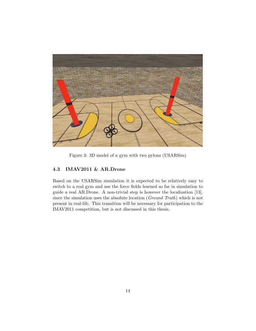
Figure 3: 3D model of a gym with two pylons (USARSim)

4.3 IMAV2011 & AR.Drone

Based on the USARSim simulation it is expected to be relatively easy toswitch to a real gym and use the force fields learned so far in simulation toguide a real AR.Drone. A non-trivial step is however the localization [13],since the simulation uses the absolute location (Ground Truth) which is notpresent in real-life. This transition will be necessary for participation to theIMAV2011 competition, but is not discussed in this thesis.

14

5 Results

The results of force fields are best shown in figures. Interesting aspects willbe discussed in the next section.

5.1 Simple Simulation

A classical example of a field with one goal position and some obstacles wasshown in figure 1 (section 3). Five circle-shaped obstacles were created withtwo different radii. All have a (quadratic inversely proportional) repellingforce, some have a rotational bias. The goal has a attractive force which is ofconstant length. The drone is released on random locations not containingan object. In the initial force field shown in the figure, one hundred randomlychosen locations (not inside objects) result in the drone finding the goal.Changing the strength of the different force setting does not really matterfor this result as long as no local minima are being created. These couldonly occur if two repelling forces and the goal-directed force sum to a vectorpointing, which could be the case depending on the relative strength of theattracting and repelling forces, as well as the density of the objects.

For the “Figure-Eight” task two circle-shaped obstacles are created (thepylons) and a rectangular-shaped obstacle is used for the walls. Repellingforces are added, as well as a rotational bias for both pylons (one clockwiseand one anti-clockwise) to prevent the drone from passing the pylon at thewrong side (flying “Figure-Zeros”). Apparently no attracting force is neededand the drone starts flying figure-eights as soon as it is released somewherein the force field. Shown in figure 4 is the initial force field with the yellowcolored force vectors used in the first run.

After the initial force field is set, the drone is released at the center of thefigure-eight. The drone then flies continuously figure-eights. When an objectis hit, the drone is restored at it’s original starting point with zero speed.

A typical result of the reinforcement learning algorithm applied to the initialforce field is shown in figures 5(a) and 5(b). For the learning part, γ = 0.6,α = 0.4, ε = 0.3, H = 10, 1200 force vectors are used and 250 stagetransitions were made (making 125 figure-eights). A constant speed causedthe vectors getting equal length. Following the vectors shows a shorter andthus improved path nearby the pylons8, while still containing trained vectors

8At the time these results were saved, the simple simulation did not incorporated the

15

Figure 4: Figure-Eight initial force field (simple simulation)

in wider paths which were reached due to exploration.

The (potential) values for the force vectors are shown as the vector color,with colors ranging from light blue for expected return 1 to light purple forexpected return -1.

To test whether there actually is improvement in round time another simu-lation is run with the (more common) parameter values γ = 0.9 and α = 0.2(resulting in less extreme vector improvements per round). During learningthe time is measured between two stage transitions with a total of 600 tran-sitions (thus 300 figure-eight’s). After each one hundred stages of learning,the update algorithm is paused and a test of 40 stages (20 figure-eight’s)without exploration is executed. For each of seven tests the mean durationof a stage is calculated. The stage durations during learning are shown infigure 6 (the test runs are thus not shown); the means with the standarddeviation of the 40 test runs (which where thus independent of the learningtrials) are shown in table 5.1.

size of the AR.Drone, therefore the force field vectors allow for paths at small distancesfrom the pylons

16

The algorithm seems to have a relatively big improvement at the start. Thepeeks in figure 6 at the very beginning are caused by the AR.Drone flyingan extra circle around the ‘current’ pole, which seems to stop after 25 trials.After one hundred trials learning seems to progress slowly during the restof the simulation.

Figure 6: Learning curve (durations of stages during learning)

17

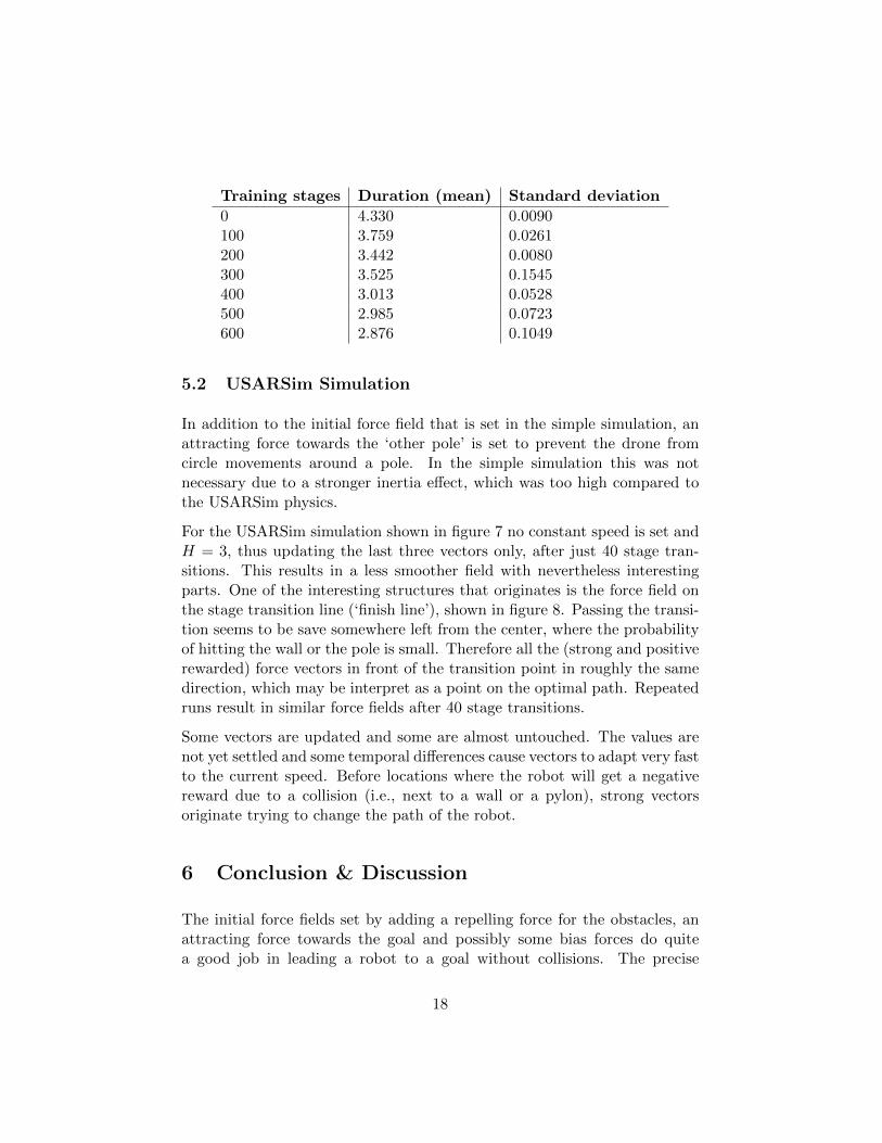
Training stages Duration (mean) Standard deviation

0 4.330 0.0090100 3.759 0.0261200 3.442 0.0080300 3.525 0.1545400 3.013 0.0528500 2.985 0.0723600 2.876 0.1049

5.2 USARSim Simulation

In addition to the initial force field that is set in the simple simulation, anattracting force towards the ‘other pole’ is set to prevent the drone fromcircle movements around a pole. In the simple simulation this was notnecessary due to a stronger inertia effect, which was too high compared tothe USARSim physics.

For the USARSim simulation shown in figure 7 no constant speed is set andH = 3, thus updating the last three vectors only, after just 40 stage tran-sitions. This results in a less smoother field with nevertheless interestingparts. One of the interesting structures that originates is the force field onthe stage transition line (‘finish line’), shown in figure 8. Passing the transi-tion seems to be save somewhere left from the center, where the probabilityof hitting the wall or the pole is small. Therefore all the (strong and positiverewarded) force vectors in front of the transition point in roughly the samedirection, which may be interpret as a point on the optimal path. Repeatedruns result in similar force fields after 40 stage transitions.

Some vectors are updated and some are almost untouched. The values arenot yet settled and some temporal differences cause vectors to adapt very fastto the current speed. Before locations where the robot will get a negativereward due to a collision (i.e., next to a wall or a pylon), strong vectorsoriginate trying to change the path of the robot.

6 Conclusion & Discussion

The initial force fields set by adding a repelling force for the obstacles, anattracting force towards the goal and possibly some bias forces do quitea good job in leading a robot to a goal without collisions. The precise

18

parameter values do not seem to have much impact on the goal-findingability of the robot. However, the path is not optimal and improving theinitial field could (theoretically) solve some well-known limitations[10] of thePotential field method:

• Local minima problem and the inability to navigate betweennarrowly spaced obstacles, which could both be solved by usingexploration to find out the best way out and updating the force vectors

• Inertia problem which could be solved by negative reward, causingthe possible passed negative vectors (due to inertia) to increase theirstrength

Reinforcement learning is an intuitive way to solve learning problems wheresetting up a reward function is easy, whereas the optimal solution is not yetknown. Therefore, we tried to incorporate the potential field method andreinforcement learning into a framework for navigation tasks.

The improved force fields show some interesting characteristics, which wewill discuss now.

First of all it seems the (potential) values of the vectors are plausible and,after more than a hundred figure-eights, cause a smooth landscape of hillson state transitions and valleys around walls. The values could be updateseven faster by using the history of visited vectors and corresponding speedvectors and immediate reward values.

However, before the vectors update to a smooth vector field, hundreds oftrials must be made, making the availability of a simulation environment apre. Some irregularities arise as long as the values are not settled to a stablelandscape. Using a constant speed ends in vectors with equal length, whilea variable speed gives vectors with variable length; some longer and thuscausing areas with fast moving and areas with slow moving.

The duration tests of figure-eight flights during learning as shown in figure6 show a slowly descending curve. The tests executed between the learn-ing sessions show a descending trend too with multiple times the standarddeviation in decrease each next test. The only increase in duration has astandard deviation that is more than the increase. Thus, it seems plausi-ble to state that the learning algorithm as presented in this thesis indeedimproves the path of a drone in the “Figure-Eight” task.

The USARSim result seems to show similar initial results, suggesting thatthe physics in the simple simulation were reasonable except for the inertia

19

strength. Although experiments with a lot more trials are only shown inboth figures and statistically for the simple simulation (which could be ac-celerated), it is likely, but not guaranteed, to converge to a smooth vectorfield with better paths as happened in the simple simulation.

7 Future Research

Future Research could focus on two different aspects.

Localization The force field contains force vectors on different locationsand needs to know which force vector to use at each moment. In the sim-ulations we used the absolute position, but in real life we don’t know thisposition that certain. A transition has to be made to this uncertain world.For localization it may be enough to use a map of the floor. Since the wholelevel is in a static, known environment, it is reasonable to presume it pos-sible to present a floor map to the robot. Alternatively this map could bemade by the robot by stitching together floor snapshots. In [13] it is shownthat a reasonable visual floor map could be created using the AR.Drone ifenough texture is present. Another possibility is the use of an algorithmbased on SLAM, with the poles as obvious landmarks. Scale is not relevant,as long as the mapping from the map to the vectors is possible.

Another option is using features from sensors like cameras or sonar as ab-stract input for the state representation, which replaces the location repre-sentation. For example, the width of the nearest pole could be enough toboth set a reasonable initial force and learn a better force vector identifiedby that feature.

Mathematical improvements It is yet not known if the proposed methodwill converge mathematically to the optimal solution (‘policy’). Furthermathematical work could be done to prove (or disprove) this.

At the moment, each force vector contains an additional value. Both a valueupdate and a vector update exist. It would be mathematically advantageousto incorporate these updates into one update on one data structure. Forexample, when using a constant speed, the norm of the vector could be usedas value, or as the temporal difference. Further research could develop one

20

coherent update, that may look like or may not look like the potential forcefields where we started this journey.

References

[1] J.R. Andrews and N. Hogan. Impedance control as a framework forimplementing obstacle avoidance in a manipulator. MIT, Dept. of Me-chanical Engineering; American Control Conference, 1983.

[2] J. Borenstein and Y. Koren. Real-time obstacle avoidance for fast mo-bile robots. IEEE Transactions On Systems, Man and Cybernetics,1989.

[3] R.A. Brooks. A robust layered control system for a mobile robot. IEEEJournal of Robotics and Automation, 1986.

[4] Wolfram Burgard, Armin B. Cremers, Dieter Fox, Dirk Hahnel, Ger-hard Lakemeyer, Dirk Schulz, Walter Steiner, and Sebastian Thrun.Experiences with an interactive museum tour-guide robot. ArtificialIntelligence, 1999.

[5] H.M. Choset et al. Principles oof Robot Motion: theory, algorithms,and implementation. MIT press, 2005.

[6] Dieter Foxy, Wolfram Burgardy, and Sebastian Thrun. The dynamicwindow approach to collision avoidance. Robotics & Automation Mag-azine, 1997.

[7] S.S. Ge and Y.J. Cui. New potential functions for mobile robot pathplanning. IEEE Transactions On Systems, Man and Cybernetics, 2000.

[8] R. Jurriaans. Optical flow based obstacle avoidance for real world au-tonomous aerial navigation tasks. Bachelor Thesis, 2011.

[9] L.P. Kaebling, M.L. Littman, and A.W. Moore. Reinforcement learn-ing: A survey. Journal of Artificial Intelligence Research, 1996.

[10] Y. Koren and J. Borenstein. Potential field methods and their inherentlimitations for mobile robot navigation. In Robotics and Automation,1991.

[11] XIE Li-juan, XIE Guang-rong, CHEN Huan-wen, and LI Xiao-li. Anovel artificial potential field-based reinforcement learning for mobile

21

robotics in ambient intelligence. International Journal of Robotics andAutomation, 2009.

[12] R. S. Sutton and A. Barto. Reinforcement Learning: An introduction.Cambridge: MIT Press, 1998.

[13] A. Visser, N. Dijkshoorn, M. van der Veen, and R. Jurriaans. Closingthe gap between simulation and reality in the sensor and motion modelsof an autonomous ar.drone. Accepted for publication at the IMAV2011conference, 2011.

22

(a) Left to Right

(b) Right to Left

Figure 5: Figure-Eight after 250 stage transitions (simple simulation)

23

Figure 7: USARSim result

Figure 8: USARSim result, stage transition area

24