I. Matta, “Optimizing and Modeling Dynamics in Networks”, in H. Haddadi, O. Bonaventure (Eds.), Recent Advances inNetworking, (2013), pp. 163-220. Licensed under a CC-BY-SA Creative Commons license.

Optimizing and Modeling Dynamics in Networks

Ibrahim Matta

1 IntroductionThe Internet has grown very large. No one knows exactly how large, but rough estimates indicate billions ofusers (around 1.8B in 2009, according to eTForecasts [4]), hundreds of millions of web sites (over 200M inFebruary 2009, according to Netcraft [19]), and hundreds of billions of web pages (over 240B, according tothe Internet archive [1]). The Internet is also very dynamic — users log in and out, new services get added,routing policies change, normal traffic gets mixed with denial-of-service (DoS) attack traffic, etc.

An important question is: How do we manage such a huge and highly dynamic structure like the Internet?As a corollary, how can we build a network of the future unless we understand the steady-state and dynamicsof what we build?

In this chapter, we resort to two mathematical frameworks: optimization theory to study optimal steadystates of networks, and control theory to study the dynamic behavior of networks as they evolve towardsteady state. Our emphasis will be on congestion control using the notion of prices to model the level ofcongestion, such as delays and losses, observed by users or traffic sources.

Expected Background: We assume basic background in calculus and algebra. We also assume basicknowledge of systems modeling, optimization theory, Laplace transforms, and control theory — Keshav’stextbook [13] provides an excellent source for these mathematical foundations, in particular, chapters 4, 5,and 8. Basic knowledge of Internet’s Transmission Control Protocol (TCP) [11], namely Reno and Vegas[15] versions, as well as queue management schemes, namely Random Early Drop (RED) [6], should behelpful. This chapter briefly covers needed background material to serve as a refresher or quick reference.The material of this chapter has been used at Boston University in a second (advanced) networking coursetaken by senior undergraduate and graduate students.

Contribution and Outline: The purpose of this chapter is to make the application of optimization andcontrol theory to congestion control more accessible through intuitive explanations and simple control ap-plications, using examples from Internet’s protocols. This chapter has been largely influenced by the workof Frank Kelly [12], which introduces the notion of “prices” and “user utility”, the work by R. Srikant [24],which discusses the dynamics of user (traffic source) and network adaptations, and control theory texts andnotes (e.g., [20, 16]). The exposition here attempts to tie these various mathematical models and techniquesthrough simple running examples and illustrations, modeling the dynamics of both flow control and routing.

We start by motivating the network control problem using analogy to the problem of producing, pricing,and consuming gas/oil (Section 2). We introduce several examples of optimally allocating resources (linkbandwidth) to users (traffic sources), resulting in different notions of fairness. We then introduce dynamicequations that model source and link adaptation algorithms (Section 3). Since these are generally non-linearequations, we review the technique of linearization and how classical (linear) control theory can be used to

study stability and transient performance (Section 4). We use as a running example, a Vegas-like systemcontrolled using different types of well-established controllers. Using linear approximation around a certainoperating point, we can only study so-called local stability.

To study general (global) stability of non-linear models, we introduce the control-theoretic Lyapunovmethod (Section 5). We also show how the control-theoretic Nyquist stability method can be applied tothe linearized model to study the impact of delay in feedback (i.e., measurements of the current state ofthe system). The material on the Nyquist method is a bit more advanced and can be skipped on a firstreading. We generalize the notion of stability by introducing the concept of contractive mapping, and extendits application to routing dynamics (Section 6).

Finally, we provide two case studies that apply control-theoretic techniques introduced in this chapter:the first study investigates stability under class-based scheduling of rate-adaptive traffic flows (Section 7),and the second study investigates stability of data transfer over a dynamic number of rate-adaptive transportconnections (Section 8). These case studies can be skipped on a first reading.

The chapter concludes with a set of exercises (Section 9) and their solutions (Section 10).

2 Network Control as an Optimization ProblemIn this section, we describe Frank Kelly’s optimization framework [12], which models users’ expectations(requirements) with utility functions, and network congestion signals (e.g., loss, delay) as prices. The net-work is shown to allocate transmission rates (throughputs) to users (flows) in such a way as to meet somefairness objective.

The objective of a user, or what makes the user happy, can be mathematically modeled as a utilityfunction. For example, drivers observe the“price” of transportation and make one of many possible decisions:drive, take the subway instead, walk, bike, or stay home. The decision may involve several factors like theprice of gas, convenience, travel time, etc. For example, if it rains, you might decide to drive to work, or youmight decide to walk to work to save money and can then afford to go to the movies later in the week. Ofcourse, how much driving a person does, is affected by all sorts of factors and user priorities are unknown tothe system of gas stations and oil companies. But, each driver has her own utility!

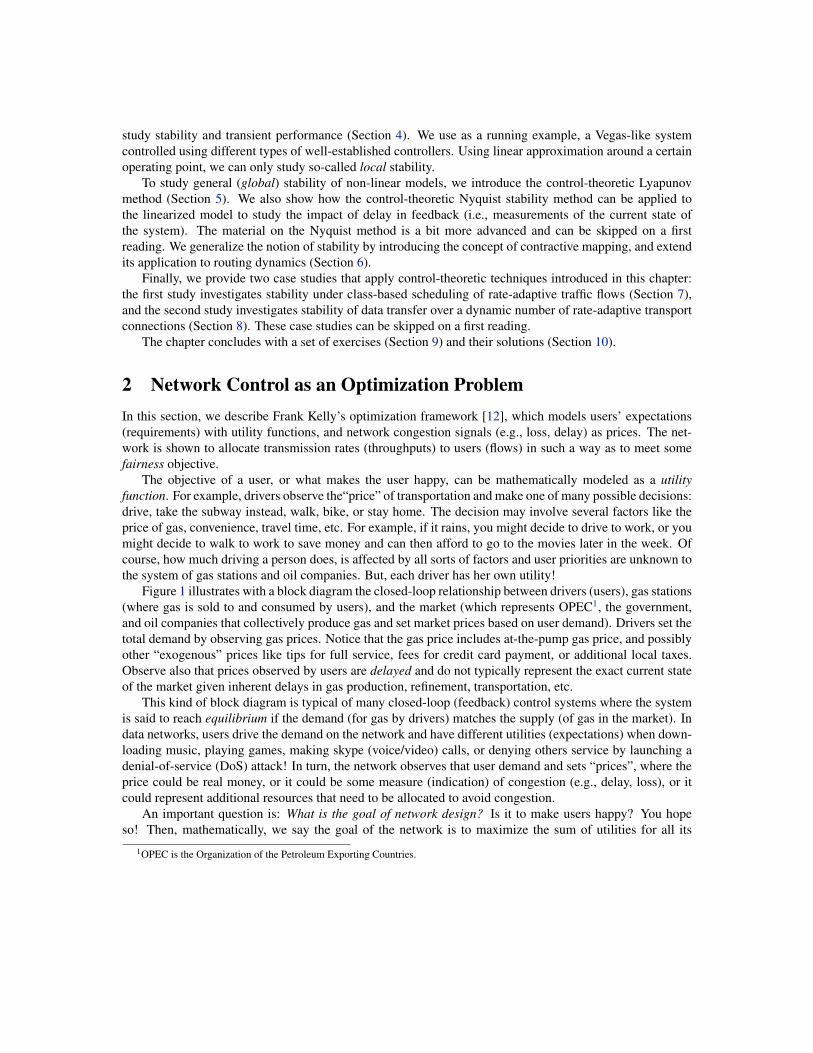
Figure 1 illustrates with a block diagram the closed-loop relationship between drivers (users), gas stations(where gas is sold to and consumed by users), and the market (which represents OPEC1, the government,and oil companies that collectively produce gas and set market prices based on user demand). Drivers set thetotal demand by observing gas prices. Notice that the gas price includes at-the-pump gas price, and possiblyother “exogenous” prices like tips for full service, fees for credit card payment, or additional local taxes.Observe also that prices observed by users are delayed and do not typically represent the exact current stateof the market given inherent delays in gas production, refinement, transportation, etc.

This kind of block diagram is typical of many closed-loop (feedback) control systems where the systemis said to reach equilibrium if the demand (for gas by drivers) matches the supply (of gas in the market). Indata networks, users drive the demand on the network and have different utilities (expectations) when down-loading music, playing games, making skype (voice/video) calls, or denying others service by launching adenial-of-service (DoS) attack! In turn, the network observes that user demand and sets “prices”, where theprice could be real money, or it could be some measure (indication) of congestion (e.g., delay, loss), or itcould represent additional resources that need to be allocated to avoid congestion.

An important question is: What is the goal of network design? Is it to make users happy? You hopeso! Then, mathematically, we say the goal of the network is to maximize the sum of utilities for all its

1OPEC is the Organization of the Petroleum Exporting Countries.

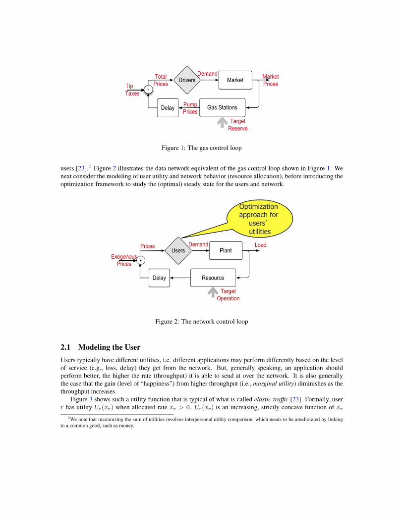
Figure 1: The gas control loop

users [23].2 Figure 2 illustrates the data network equivalent of the gas control loop shown in Figure 1. Wenext consider the modeling of user utility and network behavior (resource allocation), before introducing theoptimization framework to study the (optimal) steady state for the users and network.

Figure 2: The network control loop

2.1 Modeling the UserUsers typically have different utilities, i.e. different applications may perform differently based on the levelof service (e.g., loss, delay) they get from the network. But, generally speaking, an application shouldperform better, the higher the rate (throughput) it is able to send at over the network. It is also generallythe case that the gain (level of “happiness”) from higher throughput (i.e., marginal utility) diminishes as thethroughput increases.

Figure 3 shows such a utility function that is typical of what is called elastic traffic [23]. Formally, userr has utility Ur(xr) when allocated rate xr > 0. Ur(xr) is an increasing, strictly concave function of xr

2We note that maximizing the sum of utilities involves interpersonal utility comparison, which needs to be ameliorated by linkingto a common good, such as money.

(see Figure 4). And the derivative Ur(xr)→∞ as xr → 0, and Ur(xr)→ 0 as xr →∞. Throughout thischapter we assume strictly concave utilities.

Figure 3: Concave utility function

Figure 4: Concave function. A function f(.) is said to be concave if f(αx1 + (1− α)x2) ≥ αf(x1) + (1−α)f(x2), i.e., for any two points x1 and x2, the straight line that connects f(x1) and f(x2) is always belowor equal to the function f(.) itself. Note that a differentiable concave function has a maximum value at somepoint xmax, and that the derivative f(xmax) = 0. A strictly concave function would have a strict inequality,whereas a convex function has a cup-like shape and has a minimum instead.

2.2 Modeling the NetworkWe consider a network of J resources, e.g., transmission links as they are typically considered the bottleneck.We denote by R the set of all possible routes, and we assume that each user (source-destination traffic flow)is assigned to exactly one route r (i.e., static single-path routing)3. We then define a 0-1 routing matrix Asuch that:

ajr =

{1 if resource j is on route r0 otherwise

Figure 5 shows an example with three users over a network of seven links: the first user (“blue” flow) usesthe route made of links 1, 4, and 6; the second user (“red” flow) uses the route made of links 2, 5, and 7; andthe third user (“green” flow) uses the route made of links 1, 4, and 7. So the routing matrix has seven rowsand three columns.

3Given each user has one flow over a single path, we use the terms “user”, “flow”, and “route” interchangeably.

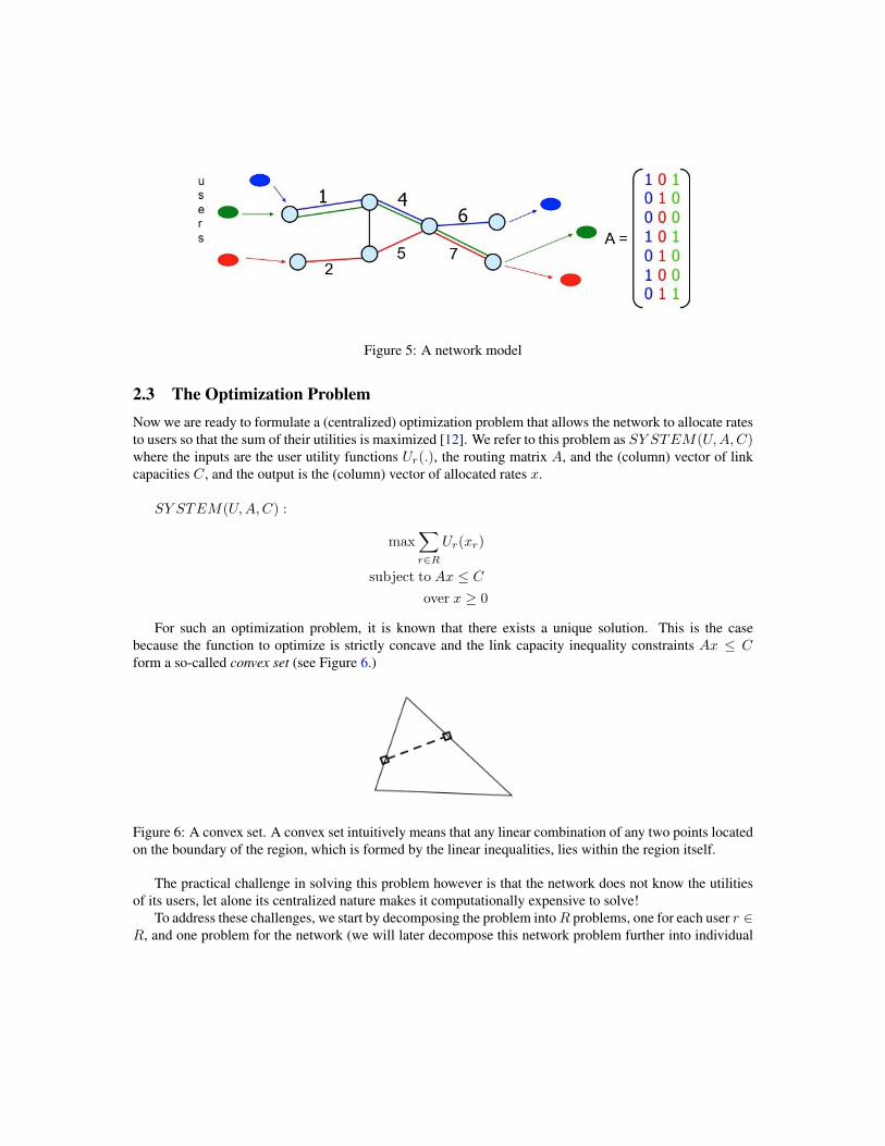
Figure 5: A network model

2.3 The Optimization ProblemNow we are ready to formulate a (centralized) optimization problem that allows the network to allocate ratesto users so that the sum of their utilities is maximized [12]. We refer to this problem as SY STEM(U,A,C)where the inputs are the user utility functions Ur(.), the routing matrix A, and the (column) vector of linkcapacities C, and the output is the (column) vector of allocated rates x.

SY STEM(U,A,C) :

max∑r∈R

Ur(xr)

subject to Ax ≤ Cover x ≥ 0

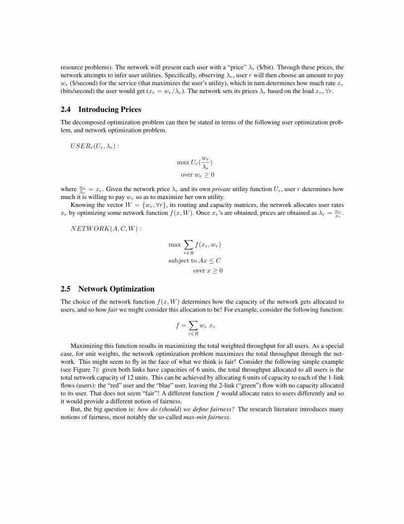
For such an optimization problem, it is known that there exists a unique solution. This is the casebecause the function to optimize is strictly concave and the link capacity inequality constraints Ax ≤ Cform a so-called convex set (see Figure 6.)

Figure 6: A convex set. A convex set intuitively means that any linear combination of any two points locatedon the boundary of the region, which is formed by the linear inequalities, lies within the region itself.

The practical challenge in solving this problem however is that the network does not know the utilitiesof its users, let alone its centralized nature makes it computationally expensive to solve!

To address these challenges, we start by decomposing the problem intoR problems, one for each user r ∈R, and one problem for the network (we will later decompose this network problem further into individual

resource problems). The network will present each user with a “price” λr ($/bit). Through these prices, thenetwork attempts to infer user utilities. Specifically, observing λr, user r will then choose an amount to paywr ($/second) for the service (that maximizes the user’s utility), which in turn determines how much rate xr(bits/second) the user would get (xr = wr/λr). The network sets its prices λr based on the load xr, ∀r.

2.4 Introducing PricesThe decomposed optimization problem can then be stated in terms of the following user optimization prob-lem, and network optimization problem.

USERr(Ur, λr) :

max Ur(wrλr

)

over wr ≥ 0

where wr

λr= xr. Given the network price λr and its own private utility function Ur, user r determines how

much it is willing to pay wr so as to maximize her own utility.Knowing the vector W = {wr,∀r}, its routing and capacity matrices, the network allocates user rates

xr by optimizing some network function f(x,W ). Once xr’s are obtained, prices are obtained as λr = wr

xr.

NETWORK(A,C,W ) :

max∑r∈R

f(xr, wr)

subject to Ax ≤ Cover x ≥ 0

2.5 Network OptimizationThe choice of the network function f(x,W ) determines how the capacity of the network gets allocated tousers, and so how fair we might consider this allocation to be! For example, consider the following function:

f =∑r∈R

wr xr

Maximizing this function results in maximizing the total weighted throughput for all users. As a specialcase, for unit weights, the network optimization problem maximizes the total throughput through the net-work. This might seem to fly in the face of what we think is fair! Consider the following simple example(see Figure 7): given both links have capacities of 6 units, the total throughput allocated to all users is thetotal network capacity of 12 units. This can be achieved by allocating 6 units of capacity to each of the 1-linkflows (users): the “red” user and the “blue” user, leaving the 2-link (“green”) flow with no capacity allocatedto its user. That does not seem “fair”! A different function f would allocate rates to users differently and soit would provide a different notion of fairness.

But, the big question is: how do (should) we define fairness? The research literature introduces manynotions of fairness, most notably the so-called max-min fairness.

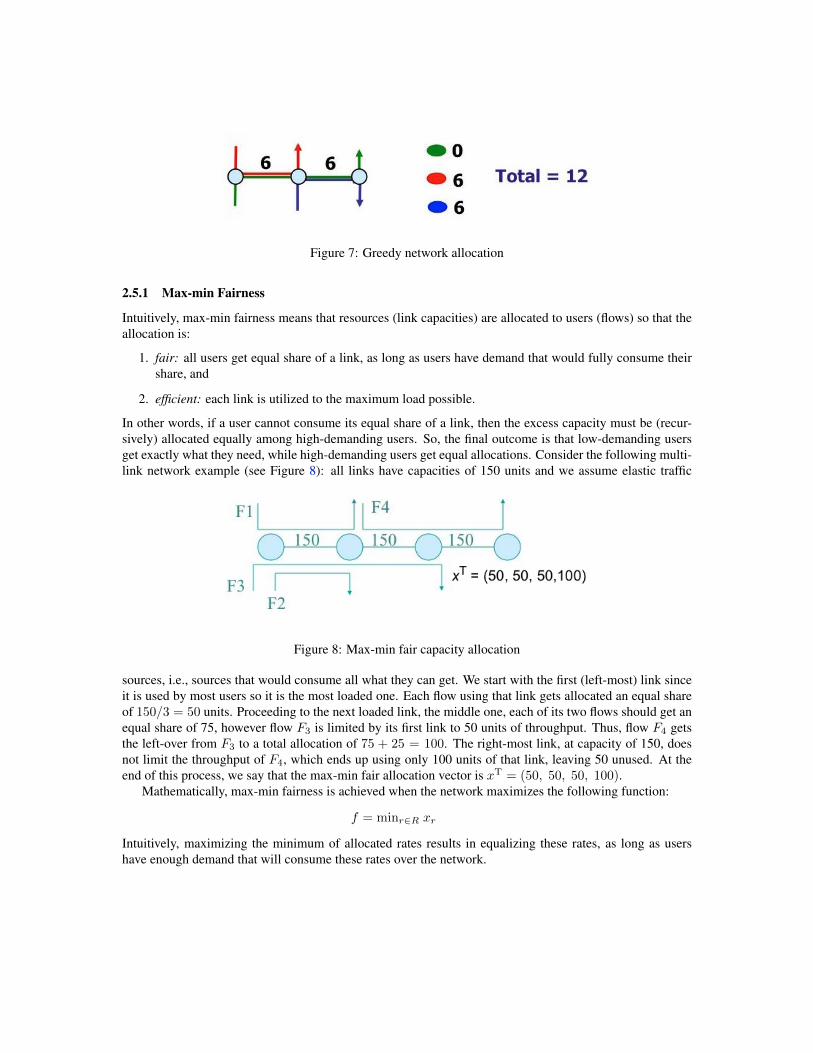
Figure 7: Greedy network allocation

2.5.1 Max-min Fairness

Intuitively, max-min fairness means that resources (link capacities) are allocated to users (flows) so that theallocation is:

1. fair: all users get equal share of a link, as long as users have demand that would fully consume theirshare, and

2. efficient: each link is utilized to the maximum load possible.

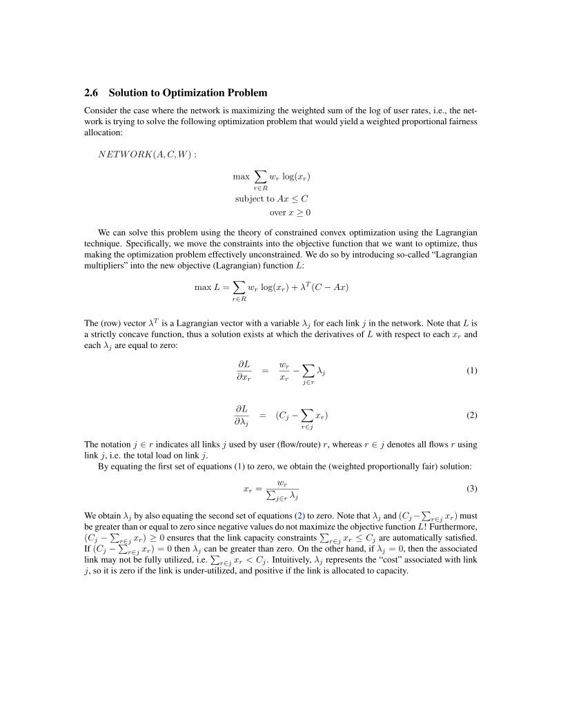
In other words, if a user cannot consume its equal share of a link, then the excess capacity must be (recur-sively) allocated equally among high-demanding users. So, the final outcome is that low-demanding usersget exactly what they need, while high-demanding users get equal allocations. Consider the following multi-link network example (see Figure 8): all links have capacities of 150 units and we assume elastic traffic

Figure 8: Max-min fair capacity allocation

sources, i.e., sources that would consume all what they can get. We start with the first (left-most) link sinceit is used by most users so it is the most loaded one. Each flow using that link gets allocated an equal shareof 150/3 = 50 units. Proceeding to the next loaded link, the middle one, each of its two flows should get anequal share of 75, however flow F3 is limited by its first link to 50 units of throughput. Thus, flow F4 getsthe left-over from F3 to a total allocation of 75 + 25 = 100. The right-most link, at capacity of 150, doesnot limit the throughput of F4, which ends up using only 100 units of that link, leaving 50 unused. At theend of this process, we say that the max-min fair allocation vector is xT = (50, 50, 50, 100).

Mathematically, max-min fairness is achieved when the network maximizes the following function:

f = minr∈R xr

Intuitively, maximizing the minimum of allocated rates results in equalizing these rates, as long as usershave enough demand that will consume these rates over the network.

2.5.2 Proportional Fairness

Another equally popular fairness definition is the so-called (weighted) proportional fairness. This notion offairness is achieved when the network maximizes the following function:

f =∑r∈R

wr log(xr)

Note that the log function is a concave, and strictly increasing function. Thus, given optimal rate allocationsolution x∗, that is feasible, i.e., x∗ ≥ 0 andA x∗ ≤ C, any other feasible solution xwill cause the aggregateproportional change

∑r∈R wr

xr−x∗rx∗r

to be less than or equal zero. To show this, for simplicity, assume oneuser and unit weight, so f(x) = log(x). Expanding f(x) into its first-order (linear) Taylor’s approximationaround x∗, we obtain:

f(x) ≈ f(x∗) + (x− x∗)f(x∗)

Given the derivative f(x∗) = 1x∗ , we have:

f(x) ≈ f(x∗) +(x− x∗)x∗

Since f is maximized at x∗, f(x∗) ≥ f(x) and so the proportional fairness condition must hold:

x− x∗

x∗≤ 0

Note that the presence of weight wr intuitively means that user (flow) r is equivalent to wr users with unitweight each.

2.5.3 General Parameterized Utility

If the network function f(x) is a function of the utilities of its users U(x), then the network is in factmaximizing a function of user utilities. Assuming each user r has unit weight wr, Ur(xr) can be generalizedas [18]:

Ur(xr) =x1−αr

1− α

where α is a parameter that determines the fairness criterion of the network. More specifically, if α → 0,then a user’s utility is linear in its allocated rate and the network is effectively maximizing the sum ofuser utilities

∑r∈R Ur(xr) =

∑r∈R xr, which in turn yields a greedy allocation that maximizes the total

throughput over the network.On the other hand, if α→ 1, then this is equivalent to a log utility, yielding proportional fair allocation.

To see this, let’s take the derivative of Ur(xr):

Ur(xr) =(1− α)x−αr

1− α→ 1

xras α→ 1

By integrating Ur(xr), we get back Ur(xr) = log(xr).Similarly, it can be shown that α → ∞ corresponds to a minimum utility, yielding a max-min fair

allocation.

2.6 Solution to Optimization ProblemConsider the case where the network is maximizing the weighted sum of the log of user rates, i.e., the net-work is trying to solve the following optimization problem that would yield a weighted proportional fairnessallocation:

NETWORK(A,C,W ) :

max∑r∈R

wr log(xr)

subject to Ax ≤ Cover x ≥ 0

We can solve this problem using the theory of constrained convex optimization using the Lagrangiantechnique. Specifically, we move the constraints into the objective function that we want to optimize, thusmaking the optimization problem effectively unconstrained. We do so by introducing so-called “Lagrangianmultipliers” into the new objective (Lagrangian) function L:

max L =∑r∈R

wr log(xr) + λT (C −Ax)

The (row) vector λT is a Lagrangian vector with a variable λj for each link j in the network. Note that L isa strictly concave function, thus a solution exists at which the derivatives of L with respect to each xr andeach λj are equal to zero:

∂L

∂xr=

wrxr−∑j∈r

λj (1)

∂L

∂λj= (Cj −

∑r∈j

xr) (2)

The notation j ∈ r indicates all links j used by user (flow/route) r, whereas r ∈ j denotes all flows r usinglink j, i.e. the total load on link j.

By equating the first set of equations (1) to zero, we obtain the (weighted proportionally fair) solution:

xr =wr∑j∈r λj

(3)

We obtain λj by also equating the second set of equations (2) to zero. Note that λj and (Cj−∑r∈j xr) must

be greater than or equal to zero since negative values do not maximize the objective functionL! Furthermore,(Cj −

∑r∈j xr) ≥ 0 ensures that the link capacity constraints

∑r∈j xr ≤ Cj are automatically satisfied.

If (Cj −∑r∈j xr) = 0 then λj can be greater than zero. On the other hand, if λj = 0, then the associated

link may not be fully utilized, i.e.∑r∈j xr < Cj . Intuitively, λj represents the “cost” associated with link

j, so it is zero if the link is under-utilized, and positive if the link is allocated to capacity.

Example: Consider the example in Figure 7 but now assume the network’s objective of proportionallyallocating its capacity, i.e.,

max f = log(x0) + log(x1) + log(x2)

subject to:

x0 + x1 ≤ 6

x0 + x2 ≤ 6

x0, x1, x2 ≥ 0

where x0, x1, and x2 are the rates allocated to the two-link flow (user), the first-link flow, and the second-linkflow, respectively. 4

Using the Lagrangian’s solution method, we obtain:

max L = log(x0) + log(x1) + log(x2) + λ1(6− (x0 + x1)) + λ2(6− (x0 + x2))

Taking derivatives, we obtain:∂L∂x0

= 1x0− (λ1 + λ2)

∂L∂x1

= 1x1− λ1

∂L∂x2

= 1x2− λ2

∂L∂λ1

= 6− (x0 + x1)

∂L∂λ2

= 6− (x0 + x2)

Equating these derivatives to zero, the last two equations show full utilization of the link capacities and thatx1 = x2, while the first three equations give the following values of xi’s:

x1 = x2 =1

λ1=

1

λ2=

1

λ

x0 =1

2λ

Substituting in the capacity equations, we obtain the price of each link λ:

1

2λ+

1

λ= 6

Thus, λ = 14 , and so x0 = 2, and x1 = x2 = 4. Note that in this optimal case, each link is fully utilized

to capacity, and the flow that traverses two links is charged twice for each link it traverses and so it getsallocated a lower rate.5 End Example.

4Note that since the objective (log) function is strictly increasing, then the xi’s should be as large as possible to consume the totalcapacity of the links, so the two inequalities on link capacities could be turned into equalities.

5As we will later see, this proportional rate allocation is what TCP Vegas [15] provides.

If the utility of each user r is a log function in its allocated rate xr, then the (weighted proportionallyfair) network solution xr = wr∑

j∈rλj

is in fact, a solution to the whole system optimization problem that

includes the network, as well as all users possibly trying to independently (in a distributed way) maximizetheir own log utilities. However, in a distributed setting, as noted earlier, even if the network knows theuser utility functions, the network allocates user rates based on their willingness to pay, wr, which might beunknown to the network. This lack of knowledge can be overcome by observing the demand behavior of theuser xr and the price λr =

∑j∈r λj , and so wr is computed as wr = xr λr. Otherwise, the network can

just assign some weights wr to users based on some preference policy.The moral of the story is that in practice, there is no central network controller that knows W and can

then allocate rates to users. Each user and each resource (link) might have its own individual controller thatwill operate independently and so we need to study the collective behavior of such composite system andanswer questions such as: Would the system converge (stabilize) to a solution in the long term (i.e., reachingsteady state)? If so, is this solution unique and how far is it from the target (optimal) operating point? Ingeneral, if the system gets perturbed, is it stable, i.e. does it converge back to steady state, and how longdoes it take to converge and how smooth or rough was that? In control-theoretic terminology, we refer tothe response to such perturbation until steady state is reached as the transient response of the system. Werefer to how far the system is from being unstable, or the magnitude of perturbation that renders the systemunstable, as stability margin.

To formally address these questions, we will resort to the modeling of user and network dynamic behav-iors, in the form of differential (or difference) equations, then use well-known control-theoretic techniquesto study the overall transient and steady-state behavior of the system.

3 The Control ProblemThe basic control problem is to control the output of a system given a certain input. For example, we wantto control the user demand (sending rate) given the observed network price (e.g., packet loss or delay).Similarly, we want to control the price advertised by a network resource given the demand (rates) of itsusers.

There is basically two kinds of control: open-loop control, and closed-loop (feedback) control. In open-loop control systems, there is no feedback about the state of the system and the output of the system iscontrolled directly by the input signal. This type of control is thus simple, but not as common as closed-loopcontrol. An example of open-loop control system is a microwave that heats food for the input (specified)duration.

Feedback (closed-loop) control is more interesting and multiple controllers may be present in the samecontrol loop. See Figure 2 where a user controller is present to control demand based on price, and a resourcecontroller is also present to control price based on demand. Feedback control makes it possible to control thesystem well even if we can’t observe or know everything, or if we make errors in our estimation (modeling)of the current state of the system, or if things change. This is because we can continually measure andcorrect (adapt) to what we observe (i.e., feedback signal). For example, in a congestion control system, wedo not need to exactly know the number of users, the arrival rate of connections, or the service rate of thebottleneck resource, since each user would adapt its demand based on its own observed (measured, fed back)price, which reflects the current overall congestion of the bottleneck resource.

Associated with feedback control is a delay to observe the feedback (measured) signal, which is referredto as feedback delay. More precisely, feedback delay refers to the time taken from the generation of acontrol signal (e.g., updated user demand) until the process/system reacts to it (e.g., demand is routed over

the network), this reaction takes effect at each resource (e.g., load is observed on each link), and this effectis fed back to the controller (e.g., price is observed by the user).

3.1 System ModelsModels of controlled systems can be classified along four dimensions:

• Deterministic versus stochastic models. The latter models capture stochastic effects like noise anduncertainties.

• Time-invariant versus time-varying models. The latter models contain system parameters that changeover time.

• Continuous-time versus discrete-time models. In the latter models, time is divided into discrete-timesteps.

• Linear versus non-linear models. The latter models contain non-linear dynamics.

In most of our treatment, we consider the simplest kind of models that are deterministic, time-invariant,continuous-time, and linear. In modeling a controlled system, we characterize the relationships amongsystem variables as a function of time, i.e., dynamic equations. See Figure 9 where functions f and h aregenerally non-linear functions. The function f models the evolution of the state of the system x as a functionof the current state and system’s input u. The function h yields system’s output y as a function of the currentstate and input values. As we will see later, for mathematical tractability, we often linearize dynamic non-linear models or we only consider operation in a linear regime, for example, we ignore non-linearity whenthe buffer goes empty or hits full capacity.

Figure 9: Typical system model

3.2 Modeling Source and Network DynamicsConsider a source r with log utility, i.e. Ur(t) = wr log(xr), and a network that allocates rates in a weightedproportional fashion. We saw earlier (cf. Section 2.6) that in steady state, the (optimal) solution (Equation3) is:

xr =wrλr

(4)

This can be re-written as wr − xrλr = 0. Also, we saw that the optimal solution ensures that each link l isfully utilized, i.e. the load (total input rate) on link l, denoted by yl =

∑s:l∈s xs, equals the link capacity cl.

The dynamics of the sources and links can then be modeled such that these steady-state user rates andlink loads are achieved. Specifically, we can write the dynamic (time-dependent) source algorithm as:

xr(t) = k[wr − xr(t)λr(t)] (5)

where k is a proportionality factor. Note that wr represents how much user r is willing to pay, whereasxr(t)λr(t) represents the cost (price) of sending at that rate. Intuitively, the user sending rate increases(decreases) when the difference between these two quantities is positive (negative). And in steady state,xr(∞)→ 0, and so we obtain the steady-state solution xr = wr

λr(as expected).

Given that the derivative of Ur(t), Ur(t) = wr

xr, the source rate adaptation algorithm can be re-written

as:

xr(t) = kxr(t)[Ur(t)− λr(t)]

xr(t) = K(t)[Ur(t)− λr(t)] (6)

Intuitively, the user increases its sending rate if the marginal utility (satisfaction) is higher than the price thatthe user will pay, otherwise the user decreases its sending rate.

We can also write a dynamic equation for the adaptation in the link price λl(t), called the link pricingalgorithm:

λl(t) = h(yl(t)− cl) (7)

where h is a proportionality factor, and the total price, λr(t), for user r, is the sum of the link prices alongthe user’s route, i.e. λr(t) =

∑l:l∈r λ

l(t). Intuitively, the link price increases if the link is over-utilized (i.e.yl(t) > cl), otherwise the link price decreases. Note that at steady state, λl(∞) → 0, and we obtain thesteady-state optimal solution yl = cl (as expected).

It turns out that the source and link algorithms, Equations 6 and 7, represent general user and resourceadaptation algorithms that collectively determine the transient and steady behavior of the whole system. Inwhat follows, we use the form of Equation 6 to reserve engineer different versions of TCP and deduce theutility function that the TCP source tries to maximize.

3.3 TCP and REDMany analytical studies considered the network system composed of TCP sources over a network of queuesthat employ a certain queue management policy. Examples of TCP variants include Reno, SACK [5],NewReno, Vegas [15], FAST [25], etc. Examples of queue management policies include Drop Tail, RED[6], REM [2], PI [10], etc. One of the most widely studied instantiation is that of TCP sources over a REDbottleneck queue — see Figure 10. We start by modeling the dynamic behavior of a TCP source, i.e., thetime-dependent relationship between its transmission window (or sending rate) and its observed loss rate ordelay (price). We do so for both TCP Reno and Vegas versions, and also deduce their utilities. Then, wemodel the buffering process inside the network (more precisely, the bottleneck queue), assuming a linearregime (i.e., ignoring non-linearities due to the buffer becoming empty or full). Using the average bufferlength, we model the dynamic behavior of RED and how it generates packet losses (or markings) as indi-cation of congestion (price). This overall model represents the closed-loop feedback system shown in theblock diagram of Figure 10, which can then be analyzed using control-theoretic techniques.

Figure 10: TCP Reno over RED feedback control system

Modeling TCP Reno: First, consider the modeling of TCP Reno, where the congestion window cwndis increased by 1/cwnd for every acknowledged TCP segment / non-loss, i.e., it is (roughly) increasedby 1 every round-trip time, and cwnd is decreased by half for every loss. Thus, we can write the followingequation for changes in the congestion window of a single TCP flow, where p is the segment loss probability:

∆cwnd =1

cwnd(1− p)− cwnd

2p

Let x denote the sending rate, and T the round-trip time, thus x = cwndT . Assuming acknowledgments

(ACKs) come equally spaced, the time between ACKs (or lack thereof) is given by Tcwnd . Thus, we can

re-write the above equation in terms of change in rate as:

d

dtcwnd(t) =

1cwnd(t) (1− p(t))− cwnd(t)

2 p(t)

Tcwnd(t)

Dividing both sides by T , we get:

d

dtx(t) =

1x(t)T 2 (1− p(t))− x(t)

2 p(t)

1x(t)

d

dtx(t) =

1

T 2(1− p(t))− x(t)

2

2p(t) (8)

Let’s denote the loss probability p(t) of TCP connection r as pr(t). pr(t) depends on the current loadon path r, and can be approximated by the sum of loss probabilities experienced on individual links j ∈ ralong the connection’s path. More specifically,

pr(t) =∑j∈r

pj(∑s:j∈s

xs(t))

Assuming small p such that (1− p) ≈ 1, we can re-write Equation 8 as follows:

d

dtx(t) =

1

T 2− x(t)

2

2p(t)

d

dtx(t) =

x(t)2

2[

2

T 2x(t)2− p(t)] (9)

Comparing Equation 9 with Equation 6, we can deduce the utility function of a TCP Reno source:

U(x) =2

T 2x2

Integrating U(x) we get:

U(x) =−2

T 2x

Observe that maximizing Reno’s utility results in minimizing the quantity 1x , which can be viewed as the

“potential delay” as it is inversely proportional to the allocated rate x. Thus, a network allocation based onsuch utility is referred to as minimum potential delay fair allocation.

Example: Revisting the example in Figure 7 but now assume the network’s objective is to allocate itscapacity according to the minimum potential delay fair allocation, i.e.,

max f =−1

x0+−1

x1+−1

x2

subject to:

x0 + x1 ≤ 6

x0 + x2 ≤ 6

x0, x1, x2 ≥ 0

where x0, x1, and x2 are the rates allocated to the two-link flow (user), the first-link flow, and the second-linkflow, respectively.

Using the Lagrangian’s solution method, we obtain:

max L =−1

x0+−1

x1+−1

x2+ λ1(6− (x0 + x1)) + λ2(6− (x0 + x2))

Taking derivatives, we obtain:∂L∂x0

= 1x20− (λ1 + λ2)

∂L∂x1

= 1x21− λ1

∂L∂x2

= 1x22− λ2

∂L∂λ1

= 6− (x0 + x1)

∂L∂λ2

= 6− (x0 + x2)

Equating these derivatives to zero, the last two equations show full utilization of the link capacities and thatx1 = x2, while the first three equations give the following values of xi’s:

x1 = x2 =1√λ1

=1√λ2

=1√λ

x0 =1√2λ

Substituting in the capacity equations, we obtain the price of each link λ = 0.08, and so x0 ≈ 2.5, andx1 = x2 ≈ 3.5.

Note that in this optimal case, each link is fully utilized to capacity, and the rate allocated to a flow isinversely proportional to the square-root of the price it observes along its path.

Note also that this captures the well-known steady-state relationship between the throughput of a TCPReno source and the inverse of the square-root of the loss probability observed by the TCP source [21]. ATCP Reno source adapting based on Equation 8 would converge to such steady-state throughput value. EndExample.

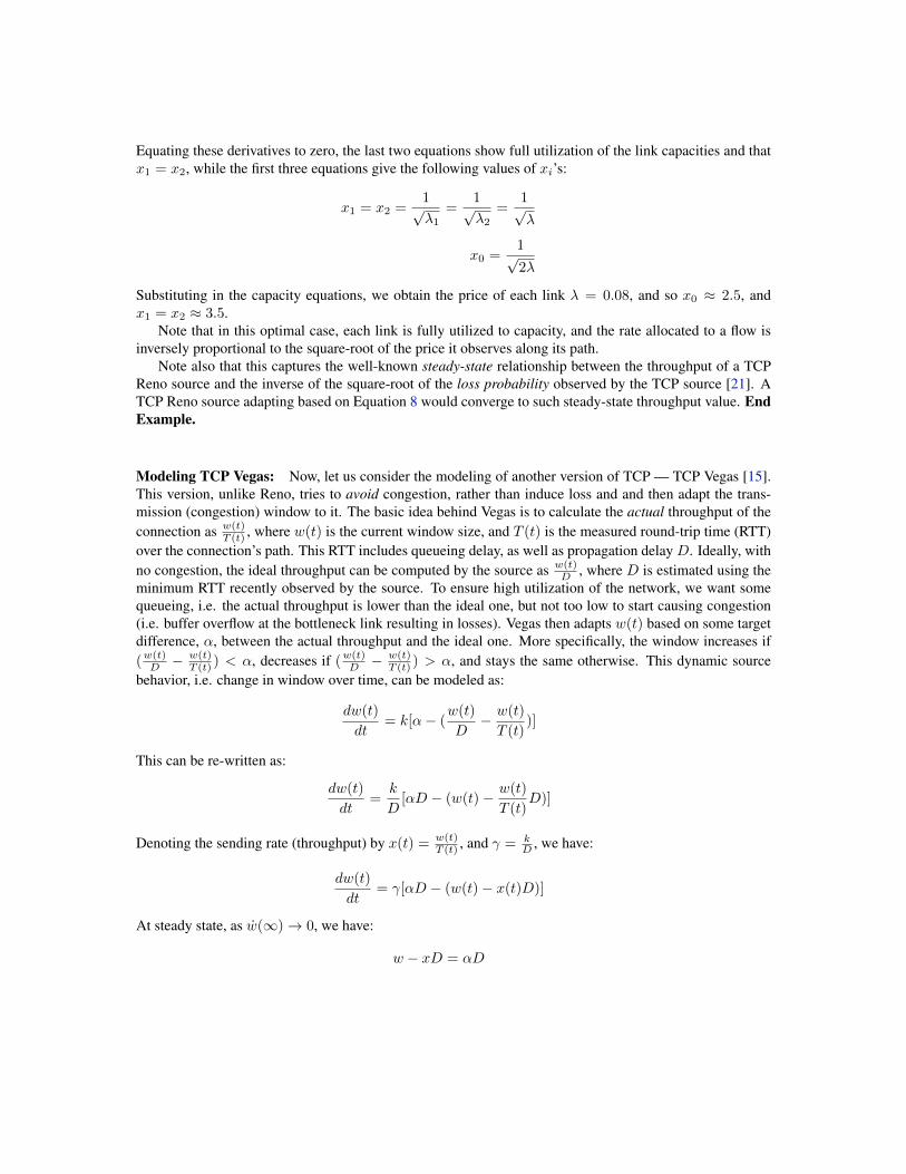
Modeling TCP Vegas: Now, let us consider the modeling of another version of TCP — TCP Vegas [15].This version, unlike Reno, tries to avoid congestion, rather than induce loss and and then adapt the trans-mission (congestion) window to it. The basic idea behind Vegas is to calculate the actual throughput of theconnection as w(t)

T (t) , where w(t) is the current window size, and T (t) is the measured round-trip time (RTT)over the connection’s path. This RTT includes queueing delay, as well as propagation delay D. Ideally, withno congestion, the ideal throughput can be computed by the source as w(t)

D , where D is estimated using theminimum RTT recently observed by the source. To ensure high utilization of the network, we want somequeueing, i.e. the actual throughput is lower than the ideal one, but not too low to start causing congestion(i.e. buffer overflow at the bottleneck link resulting in losses). Vegas then adapts w(t) based on some targetdifference, α, between the actual throughput and the ideal one. More specifically, the window increases if(w(t)D − w(t)

T (t) ) < α, decreases if (w(t)D − w(t)

T (t) ) > α, and stays the same otherwise. This dynamic sourcebehavior, i.e. change in window over time, can be modeled as:

dw(t)

dt= k[α− (

w(t)

D− w(t)

T (t))]

This can be re-written as:

dw(t)

dt=

k

D[αD − (w(t)− w(t)

T (t)D)]

Denoting the sending rate (throughput) by x(t) = w(t)T (t) , and γ = k

D , we have:

dw(t)

dt= γ[αD − (w(t)− x(t)D)]

At steady state, as w(∞)→ 0, we have:

w − xD = αD

Observe that the left-hand side represents the difference between the window size of packets injected bythe source, and the number of packets in flight / propagating along the path (represented by the productof throughput and propagation delay). Thus, the left-hand side represents the number of packets in thebottleneck queue, and αD denotes the target queue occupancy of the bottleneck link. Intuitively, Vegas triesto maintain a small number of αD packets (i.e., 1-2 packets) in the bottleneck queue to maintain both smalldelay and high (100%) utilization. Section 4 uses control theory to analyze a Vegas-like transmission model.

Given that x = w/T , we get:

xT − xD = αD

Denoting the queueing delay by Q, we have T = Q+D, and so:

xQ = αD

x =αD

Q

Comparing with Equation 4, we can deduce that the willingness to pay wr for a Vegas user r is αD and thatthe price λr experienced by the user is the queueing delay Q.

Now, to deduce the utility function that a Vegas user tries to maximize, let us write its rate adaptationequation following Equation 5:

xr(t) = k[αD − xr(t)Q(t)]

xr(t) = K(t)[αD

xr(t)−Q(t)]

Thus, comparing with Equation 6, we deduce:

Ur(t) =αD

xr(t)

Integrating, we obtain:

Ur(t) = αD log(xr(t))

Recall that maximizing such user utilities results in a weighted proportional fair allocation.

Modeling RED: Let us now consider the modeling of the buffer and associated RED queue managementalgorithm [6]. Figure 11 shows how RED tries to avoid congestion by dropping (or marking) packets withprobability pc as a (non-linear) function of the average queue length v. First, we model the evolution of thequeue length b(t) as a function of the total input rate, y(t) =

∑xs(t), and (bottleneck) link capacity, C:

b(t) = y(t)− C

Denoting by v(t), the Exponential Weighted Moving Average (EWMA) of the queue length:

v(t+ δ) = (1− α)v(t) + αb(t)

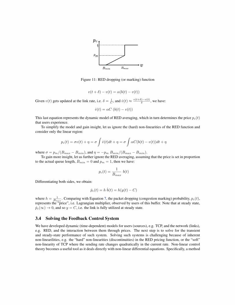
Figure 11: RED dropping (or marking) function

v(t+ δ)− v(t) = α(b(t)− v(t))

Given v(t) gets updated at the link rate, i.e. δ = 1C , and v(t) ≈ v(t+δ)−v(t)

δ , we have:

v(t) = αC (b(t)− v(t))

This last equation represents the dynamic model of RED averaging, which in turn determines the price pc(t)that users experience.

To simplify the model and gain insight, let us ignore the (hard) non-linearities of the RED function andconsider only the linear region:

pc(t) = σv(t) + η = σ

∫v(t)dt+ η = σ

∫αC(b(t)− v(t))dt+ η

where σ = pm/(Bmax −Bmin), and η = −pm Bmin/(Bmax −Bmin).To gain more insight, let us further ignore the RED averaging, assuming that the price is set in proportion

to the actual queue length, Bmin = 0 and pm = 1, then we have:

pc(t) =1

Bmaxb(t)

Differentiating both sides, we obtain:

pc(t) = h b(t) = h(y(t)− C)

where h = 1Bmax

. Comparing with Equation 7, the packet dropping (congestion marking) probability, pc(t),represents the “price”, i.e. Lagrangian multiplier, observed by users of this buffer. Note that at steady state,pc(∞)→ 0, and so y = C, i.e. the link is fully utilized at steady state.

3.4 Solving the Feedback Control SystemWe have developed dynamic (time-dependent) models for users (sources), e.g. TCP, and the network (links),e.g. RED, and the interaction between them through prices. The next step is to solve for the transientand steady-state performance of such system. Solving such systems is challenging because of inherentnon-linearilities, e.g. the “hard” non-linearities (discontinuities) in the RED pricing function, or the “soft”non-linearity of TCP where the sending rate changes quadratically in the current rate. Non-linear controltheory becomes a useful tool as it deals directly with non-linear differential equations. Specifically, a method

called Lyapunov [20] allows one to study convergence (stability) by showing that the value of some positivefunction of the state of the system continuously decreases as the system evolves over time. Finding such aLyapunov function can be challenging, and transient performance can often only be obtained by solving thesystem equations numerically.

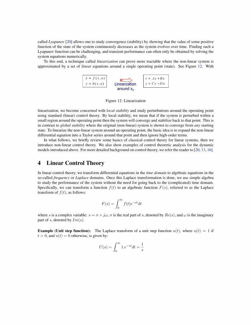
To this end, a technique called linearization can prove more tractable where the non-linear system isapproximated by a set of linear equations around a single operating point (state). See Figure 12. With

Figure 12: Linearization

linearization, we become concerned with local stability and study perturbations around the operating pointusing standard (linear) control theory. By local stability, we mean that if the system is perturbed within asmall region around the operating point then the system will converge and stabilize back to that point. This isin contrast to global stability where the original (non-linear) system is shown to converge from any startingstate. To linearize the non-linear system around an operating point, the basic idea is to expand the non-lineardifferential equation into a Taylor series around that point and then ignore high-order terms.

In what follows, we briefly review some basics of classical control theory for linear systems, then weintroduce non-linear control theory. We also show examples of control theoretic analysis for the dynamicmodels introduced above. For more detailed background on control theory, we refer the reader to [20, 13, 16].

4 Linear Control TheoryIn linear control theory, we transform differential equations in the time domain to algebraic equations in theso-called frequency or Laplace domains. Once this Laplace transformation is done, we use simple algebrato study the performance of the system without the need for going back to the (complicated) time domain.Specifically, we can transform a function f(t) to an algebraic function F (s), referred to as the Laplacetransform of f(t), as follows:

F (s) =

∫ ∞0

f(t)e−stdt

where s is a complex variable: s = σ+ jω, σ is the real part of s, denoted by Re(s), and ω is the imaginarypart of s, denoted by Im(s).

Example (Unit step function): The Laplace transform of a unit step function u(t), where u(t) = 1 ift > 0, and u(t) = 0 otherwise, is given by:

U(s) =

∫ ∞0

1.e−stdt =1

s

Example (Impulse function): The Laplace transform of a unit impulse function δ(t), where δ(t) = 1 ift = 0, and δ(t) = 0 otherwise, is given by:

U(s) =

∫ ∞0

1.e−stdt = e0 = 1

Table 1 lists basic Laplace transforms.

Table 1: Basic Laplace transforms

Impulse input: f(t) = δ(t) F (s) = 1

Step input: f(t) = a.1(t) F (s) = a/s

Ramp input: f(t) = a.t F (s) = a/s2

Exponential: f(t) = eat F (s) = 1/(s− a)

Sinusoid input: f(t) = sin(at) F (s) = a/(s2 + a2)

Table 2 lists basic composition rules, where L[f(t)] denotes the Laplace transform of f(t), i.e. F (s).

Table 2: Composition rules

Linearity: L[a f(t) + b g(t)] = aF (s) + bG(s)

Differentiation: L[df(t)/dt] = sF (s)− f(0) = sF (s) if f(0) = 0

Integration: L[∫f(τ)dτ ] = F (s)/s

Convolution: y(t) = g(t)∗u(t) =∫ t

0g(t− τ)u(τ)dτ ⇒ Y (s) = G(s)U(s)

Example: Consider the following second-order linear, time-invariant differential equation, where y(t)represents the output of a system, and u(t) represents the input:

a2y(t) + a1y(t) + a0y(t) = b1u(t) + b0u(t)

In the time domain, if we represent the system by g(t), then y(t) can be obtained by convolving u(t) withg(t), i.e. y(t) = g(t)∗u(t). This involves a complicated integration over the system responses, g(t− τ), toimpulse inputs of magnitude u(τ), for all 0 < τ < t.

Assuming y(0) = u(0) = 0, taking the Laplace transform of both sides, we obtain:

a2s2Y (s) + a1sY (s) + a0Y (s) = b1sU(s) + b0U(s)

Y (s) =(b1s+ b0)

(a2s2 + a1s+ a0)U(s) = G(s)U(s)

Thus, in the Laplace domain, the output Y (s) can be obtained by simply multiplyingG(s), called the transferfunction of the system, with U(s). We can then take the inverse Laplace transform, L−1[Y (s)], to obtainy(t), or as we will later see, we can simply analyze the stability of the system by examining the roots of thedenominator of the transfer function G(s) and their location in the complex s-domain.

Note that because Y (s) = G(s) for an impulse input, i.e. U(s) = 1, the transfer function G(s) is alsocalled impulse response function.

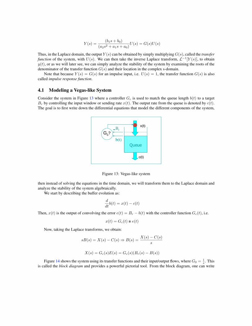
4.1 Modeling a Vegas-like SystemConsider the system in Figure 13 where a controller Gc is used to match the queue length b(t) to a targetBr by controlling the input window or sending rate x(t). The output rate from the queue is denoted by c(t).The goal is to first write down the differential equations that model the different components of the system,

Figure 13: Vegas-like system

then instead of solving the equations in the time domain, we will transform them to the Laplace domain andanalyze the stability of the system algebraically.

We start by describing the buffer evolution as:

d

dtb(t) = x(t)− c(t)

Then, x(t) is the output of convolving the error e(t) = Br − b(t) with the controller function Gc(t), i.e.

x(t) = Gc(t)∗ e(t)Now, taking the Laplace transforms, we obtain:

sB(s) = X(s)− C(s)⇒ B(s) =X(s)− C(s)

s

X(s) = Gc(s)E(s) = Gc(s)(Br(s)−B(s))

Figure 14 shows the system using its transfer functions and their input/output flows, whereG0 = 1s . This

is called the block diagram and provides a powerful pictorial tool. From the block diagram, one can write

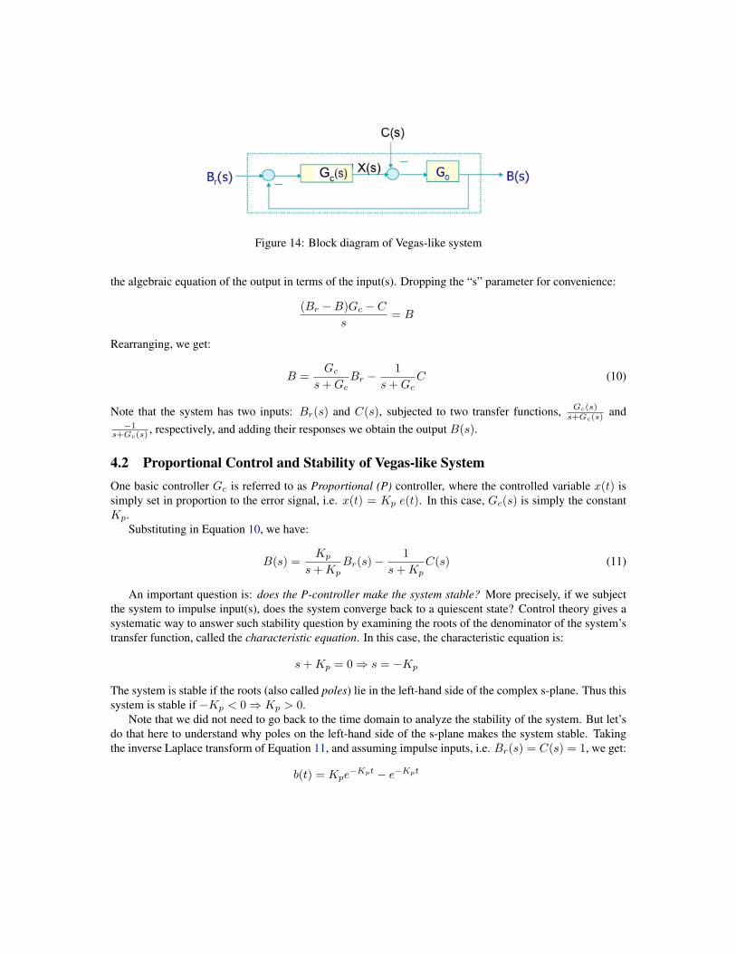
Figure 14: Block diagram of Vegas-like system

the algebraic equation of the output in terms of the input(s). Dropping the “s” parameter for convenience:

(Br −B)Gc − Cs

= B

Rearranging, we get:

B =Gc

s+GcBr −

1

s+GcC (10)

Note that the system has two inputs: Br(s) and C(s), subjected to two transfer functions, Gc(s)s+Gc(s) and

−1s+Gc(s) , respectively, and adding their responses we obtain the output B(s).

4.2 Proportional Control and Stability of Vegas-like SystemOne basic controller Gc is referred to as Proportional (P) controller, where the controlled variable x(t) issimply set in proportion to the error signal, i.e. x(t) = Kp e(t). In this case, Gc(s) is simply the constantKp.

Substituting in Equation 10, we have:

B(s) =Kp

s+KpBr(s)−

1

s+KpC(s) (11)

An important question is: does the P-controller make the system stable? More precisely, if we subjectthe system to impulse input(s), does the system converge back to a quiescent state? Control theory gives asystematic way to answer such stability question by examining the roots of the denominator of the system’stransfer function, called the characteristic equation. In this case, the characteristic equation is:

s+Kp = 0⇒ s = −Kp

The system is stable if the roots (also called poles) lie in the left-hand side of the complex s-plane. Thus thissystem is stable if −Kp < 0⇒ Kp > 0.

Note that we did not need to go back to the time domain to analyze the stability of the system. But let’sdo that here to understand why poles on the left-hand side of the s-plane makes the system stable. Takingthe inverse Laplace transform of Equation 11, and assuming impulse inputs, i.e. Br(s) = C(s) = 1, we get:

b(t) = Kpe−Kpt − e−Kpt

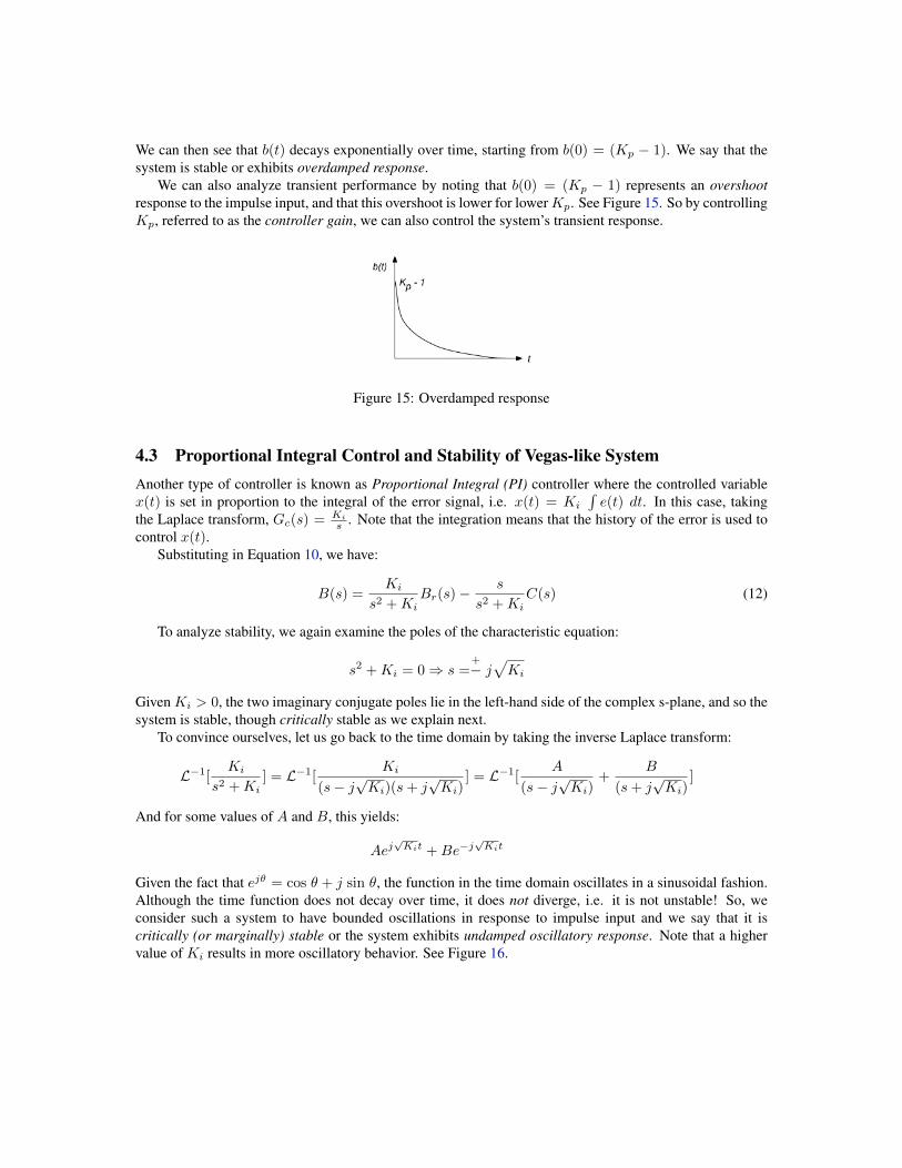
We can then see that b(t) decays exponentially over time, starting from b(0) = (Kp − 1). We say that thesystem is stable or exhibits overdamped response.

We can also analyze transient performance by noting that b(0) = (Kp − 1) represents an overshootresponse to the impulse input, and that this overshoot is lower for lowerKp. See Figure 15. So by controllingKp, referred to as the controller gain, we can also control the system’s transient response.

Figure 15: Overdamped response

4.3 Proportional Integral Control and Stability of Vegas-like SystemAnother type of controller is known as Proportional Integral (PI) controller where the controlled variablex(t) is set in proportion to the integral of the error signal, i.e. x(t) = Ki

∫e(t) dt. In this case, taking

the Laplace transform, Gc(s) = Ki

s . Note that the integration means that the history of the error is used tocontrol x(t).

Substituting in Equation 10, we have:

B(s) =Ki

s2 +KiBr(s)−

s

s2 +KiC(s) (12)

To analyze stability, we again examine the poles of the characteristic equation:

s2 +Ki = 0⇒ s =+− j√Ki

Given Ki > 0, the two imaginary conjugate poles lie in the left-hand side of the complex s-plane, and so thesystem is stable, though critically stable as we explain next.

To convince ourselves, let us go back to the time domain by taking the inverse Laplace transform:

L−1[Ki

s2 +Ki] = L−1[

Ki

(s− j√Ki)(s+ j

√Ki)

] = L−1[A

(s− j√Ki)

+B

(s+ j√Ki)

]

And for some values of A and B, this yields:

Aej√Kit +Be−j

√Kit

Given the fact that ejθ = cos θ + j sin θ, the function in the time domain oscillates in a sinusoidal fashion.Although the time function does not decay over time, it does not diverge, i.e. it is not unstable! So, weconsider such a system to have bounded oscillations in response to impulse input and we say that it iscritically (or marginally) stable or the system exhibits undamped oscillatory response. Note that a highervalue of Ki results in more oscillatory behavior. See Figure 16.

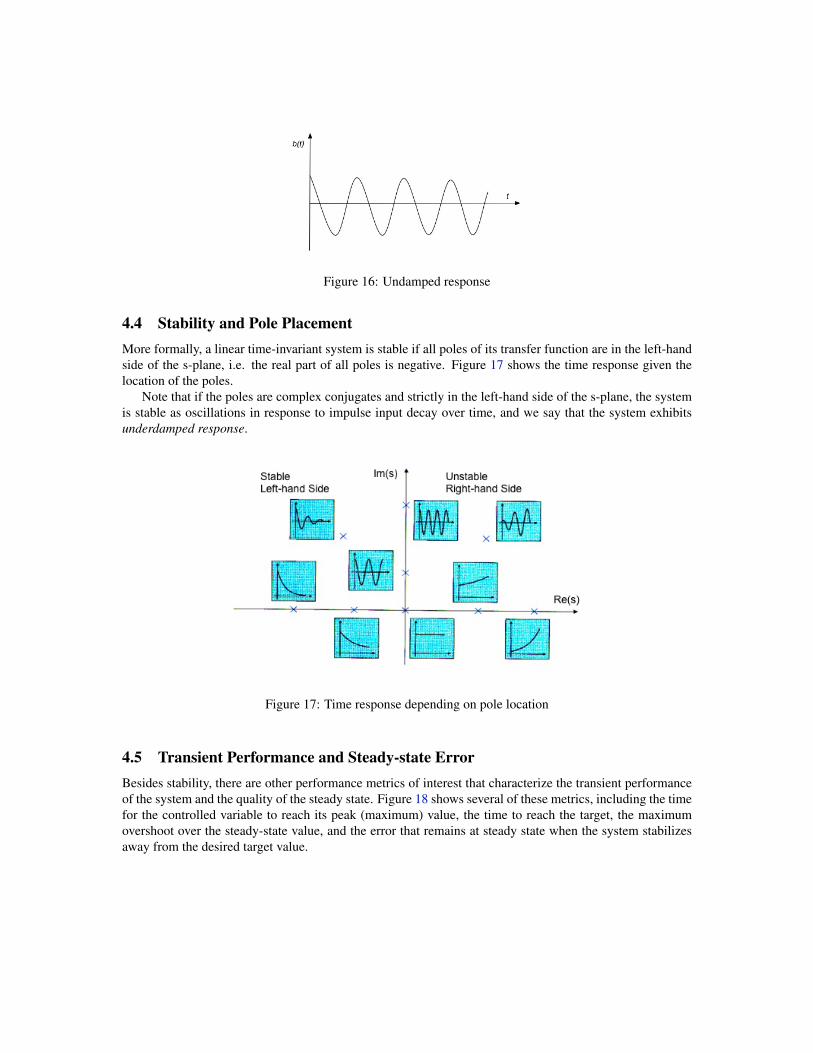
Figure 16: Undamped response

4.4 Stability and Pole PlacementMore formally, a linear time-invariant system is stable if all poles of its transfer function are in the left-handside of the s-plane, i.e. the real part of all poles is negative. Figure 17 shows the time response given thelocation of the poles.

Note that if the poles are complex conjugates and strictly in the left-hand side of the s-plane, the systemis stable as oscillations in response to impulse input decay over time, and we say that the system exhibitsunderdamped response.

Figure 17: Time response depending on pole location

4.5 Transient Performance and Steady-state ErrorBesides stability, there are other performance metrics of interest that characterize the transient performanceof the system and the quality of the steady state. Figure 18 shows several of these metrics, including the timefor the controlled variable to reach its peak (maximum) value, the time to reach the target, the maximumovershoot over the steady-state value, and the error that remains at steady state when the system stabilizesaway from the desired target value.

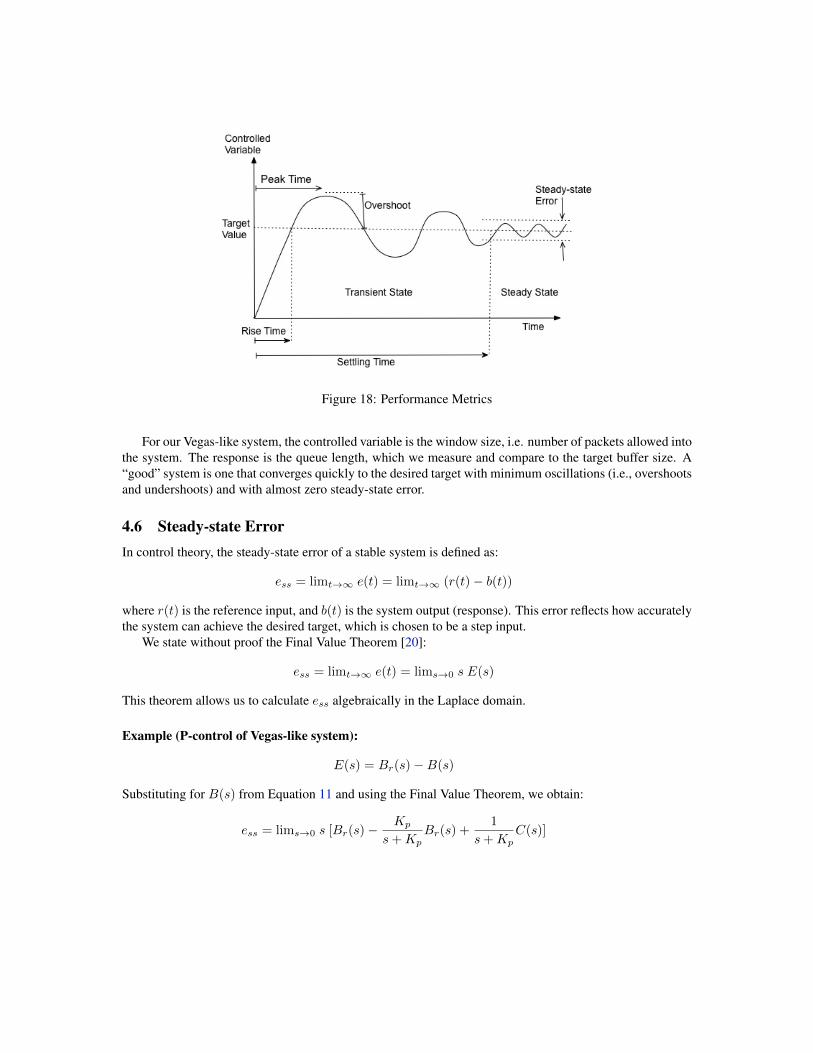
Figure 18: Performance Metrics

For our Vegas-like system, the controlled variable is the window size, i.e. number of packets allowed intothe system. The response is the queue length, which we measure and compare to the target buffer size. A“good” system is one that converges quickly to the desired target with minimum oscillations (i.e., overshootsand undershoots) and with almost zero steady-state error.

4.6 Steady-state ErrorIn control theory, the steady-state error of a stable system is defined as:

ess = limt→∞ e(t) = limt→∞ (r(t)− b(t))

where r(t) is the reference input, and b(t) is the system output (response). This error reflects how accuratelythe system can achieve the desired target, which is chosen to be a step input.

We state without proof the Final Value Theorem [20]:

ess = limt→∞ e(t) = lims→0 s E(s)

This theorem allows us to calculate ess algebraically in the Laplace domain.

Example (P-control of Vegas-like system):

E(s) = Br(s)−B(s)

Substituting for B(s) from Equation 11 and using the Final Value Theorem, we obtain:

ess = lims→0 s [Br(s)−Kp

s+KpBr(s) +

1

s+KpC(s)]

Assuming step inputs, i.e. Br(s) = Br

s and D(s) = Ds , we have:

ess = lims→0 [Br −Kp

s+KpBr +

1

s+KpC] =

C

Kp

Recall that under the P-controller, the system is (overdamped) stable, i.e. b(t) approaches the target Brwithout oscillations, however, at steady state, b(t) misses the target by C

Kpand stabilizes at a value lower

than Br. Notice that the higher the service capacity C is, the larger the steady-state error. So, to decreasethe steady-state error, the controller gain Kp could be increased. However, increasing Kp increases theovershoot. A tradeoff clearly exists between transient performance and steady-state performance, and onehas to choose Kp to balance the two and meet desired operation goals. End Example.

Example (PI-control of Vegas-like system):

E(s) = Br(s)−B(s)

Substituting for B(s) from Equation 12 and using the Final Value Theorem, we obtain:

ess = lims→0 s [Br(s)−Ki

s2 +KiBr(s) +

s

s2 +KiC(s)]

Assuming step inputs, i.e. Br(s) = Br

s and C(s) = Cs , we have:

ess = lims→0 [Br −Ki

s2 +KiBr +

s

s2 +KiC] = 0

Although the steady-state error is zero under the PI-controller, recall that the system is critically stable, i.e.it converges to the target while oscillating. Decreasing the controller gain Ki decreases these oscillations,however at the expense of longer time to reach steady state. This illustrates again the inherent tradeoffbetween transient performance and the quality of the steady state.

5 Analyzing the Stability of Non-linear SystemsAs we have seen, linear control theory can be applied to non-linear systems if we assume a small range ofoperation around which the system behavior is linear or approximately linear. This linear analysis is simpleto use, and the system, if stable, has a unique equilibrium point.

On the other hand, most control systems are non-linear, and operate over a wide range of parameters,and multiple equilibrium points may exist. In this case, non-linear control theory could be more complex touse.

In what follows, we first consider a non-linear model of the adaptation of sources and network, and use anon-linear control-theoretic stability analysis method, called Lyapunov method [20]. Then, we linearize thesystem and illustrate the application of linear control-theoretic analysis.

5.1 Solving Non-linear Differential EquationsRecall Vegas-like source adaptations from Equation 5:

dxr(t)

dt= k[wr − xr(t)pr(t)]

where pr(t) represents the total price observed by user r along its path. Note that this differential equationis non-linear since pr(t) is a function of the rates xs(t):

pr(t) =∑

link l∈route r

pl(t) =∑l∈r

pl(∑s:l∈s

xs(t))

We assume that the pricing function pl(y) is monotonically increasing in the load y.At steady state, if the system stabilizes, setting the derivatives to 0, we obtain the steady-state solution:

k[wr − xr pr] = 0⇒ xr =wrpr

=wr∑l∈r pl

To prove stability, we use the non-linear method of Lyapunov. The basic idea is to find a positive scalarfunction V (x(t)), we call the Lyapunov function, and show that the function monotonically increases (ordecreases) over time, approaching the steady-state solution.

Define V (x) as follows:

V (x) =∑r∈R

wr log(xr)−∑j∈J

∫ ∑s:j∈s

xs

0

pj(y)dy

Finding a suitable Lyapunov function that shows stability is tricky and more of an art! If you can’t findone, it does not mean that the system is not stable. Note that this V (x) has some special meaning: the firstterm represents the utility gain from making users happy, while the second term represents the cost in termsof price. So V (x) represents the net gain. Also, note that since the first term is concave because of the logfunction, and the second term is assumed to be monotonically increasing, then the resulting V (x) is concave,i.e. it has a maximum value.

To show that V (x(t)) is strictly convergent, we want to show that dV (x(t))dt > 0, which implies that

V (x(t)) strictly increases (i.e. the net gain keeps increasing over time), until the system stabilizes andreaches steady state when dV (x(t))

dt = 0 (i.e. the net gain V (x) reaches its maximum value).First, we note:

∂V (x)

∂xr=wrxr−∑j∈r

pj(∑s:j∈s

xs)

Then:

V (x(t))

dt=∑r∈R

∂V (x(t))

∂xr

dxr(t)

dt

V (x(t))

dt=∑r∈R

[wrxr−∑j∈r

pj(∑s:j∈s

xs(t))] k[wr − xr(t)pr(t)]

V (x(t))

dt=∑r∈R

k xr(t)[wrxr−∑j∈r

pj(∑s:j∈s

xs(t))]2 > 0

Observe that this non-linear stability analysis shows that the system is stable, no matter what the initialstate x(0) is. This property is referred to as global stability, which is in contract to local stability that weprove when the system is linearized locally around a certain operating point as we will see next.

5.2 Linearizing and Solving Linear Differential EquationsAs noted earlier, finding Lyapunov functions to prove global stability of non-linear control systems, evenfor simple models, is challenging. For example, consider more sophisticated models with feedback delay,different regions of TCP operation (e.g., timeouts, slow-start), queue management with different operatingregions (e.g., RED), and challenging or adversarial environments (e.g., exogenous losses over wireless linksor due to DoS attacks).

Using linearization, we can separately study simpler linear models around the different points (regions)of operation. More specifically, we linearize the system around a single operating point x∗ and study pertur-bations around x∗, i.e. if we perturb the system away from x∗ to a point x(0) such that the initial perturbationδx(0) = x(0) − x∗, we want to show that δx(t) diminishes over time and the system returns to its originalstate x∗, i.e. δx(t)→ 0. In this case, we say that the system is locally stable around x∗.

Let’s consider again the Vegas-like source adaptation and assume, for simplicity, a single user over asingle resource:

dx(t)

dt= k[w − x(t)p(x(t))]

Define the perturbation δx(t) = x(t)− x∗. Then we can write:

d(δx(t) + x∗)

dt= k[w − (δx(t) + x∗)p((δx(t) + x∗))]

Expanding the non-linear term p((δx(t) + x∗)) into its first-order Taylor series:

p((δx(t) + x∗)) ≈ p(x∗) + p(x∗)δx(t)

Substituting with this linear approximation, we get:

dδx(t)

dt= k[w − (δx(t) + x∗){p(x∗) + p(x∗)δx(t)}]

dδx(t)

dt= k[w − δx(t)p(x∗)− x∗p(x∗)− p(x∗)δ2x(t)− p(x∗)x∗δx(t)]

If x∗ is the optimal steady-state point, we know that w − x∗p(x∗) = 0 (cf. Equation 4). Also, givensmall perturbation δx(t), δ2x(t) ≈ 0. Then, we have:

dδx(t)

dt= k[−δx(t)p(x∗)− p(x∗)x∗δx(t)]

dδx(t)

dt= −k[p(x∗) + x∗p(x∗)] δx(t)

Let k[p(x∗) + x∗p(x∗)] = γ, we have:

dδx(t)

dt= −γ δx(t) (13)

This is now a linear differential equation, which unlike the original non-linear differential equation, wecan easily study using linear control-theoretic techniques, or in this simple case, solve by straightforwardintegration: ∫ t

0

d δx(t)

δx(t)= −γ

∫ t

0

dt

log(δx(t))− log(δx(0)) = −γt

log(δx(t)

δx(0)) = −γt

δx(t) = δx(0) e−γt

Note that from this time-domain analysis, the system is shown to be stable, i.e. the perturbation vanishesover time and the system returns to its original state x∗. We also observe that the system response decaysexponentially from its original perturbation δx(0), i.e. without oscillations, and so the response is classifiedas overdamped.

If the linearized differential equation modeling the system were more complicated, it is much easier totransform it into the Laplace domain and analyze the system algebraically. Denoting δx(t) by u(t), theLaplace transform of δx(t) by U(s), and taking the Laplace transform of Equation 13, we get:

s U(s)− u(0) = −γ U(s)

U(s) =u(0)

s+ γ

For stability analysis, we examine the location of the poles (roots) of the characteristic equation s+γ = 0,yielding the pole s = −γ. Since the pole is strictly in the left-side of the s-plane, given γ > 0, the system isstable and its response is overdamped.

To evaluate the steady-state error, we define the error as e(t) = u(0)−u(t), and applying the Final ValueTheorem with an impulse perturbation of magnitude u(0), i.e. U(0) = u(0), we obtain:

ess = lims→0 sE(s) = lims→0 s[u(0)− u(0)

s+ γ] = 0

So, there is no steady-state error.

5.2.1 Effect of Feedback Delay and Nyquist Stability Criterion

As we just noted above, the power of solving the linearized model in the Laplace domain comes when themodel is even slightly more complicated. For example, let us consider a feedback delay T such that Equation13 looks like:

du(t)

dt= −γ u(t− T )

Taking the Laplace transform, and noting that the Laplace transform of a delayed signal u(t − T ) ise−sTU(s), we obtain:

sU(s)− u(0) = −γ e−sTU(s)

U(s) =u(0)

s+ γ e−sT

Then, the characteristic equation is:

s+ γ e−sT = 0 (14)

which we need to solve to locate the poles and determine the stability of the system.To solve such characteristic equation, we resort to another control-theoretic method called the Nyquist

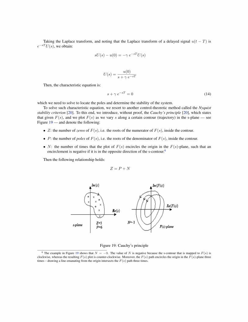
stability criterion [20]. To this end, we introduce, without proof, the Cauchy’s principle [20], which statesthat given F (s), and we plot F (s) as we vary s along a certain contour (trajectory) in the s-plane — seeFigure 19 — and denote the following:

• Z: the number of zeros of F (s), i.e. the roots of the numerator of F (s), inside the contour.

• P : the number of poles of F (s), i.e. the roots of the denominator of F (s), inside the contour.

• N : the number of times that the plot of F (s) encircles the origin in the F (s)-plane, such that anencirclement is negative if it is in the opposite direction of the s-contour.6

Then the following relationship holds:

Z = P +N

Figure 19: Cauchy’s principle

6 The example in Figure 19 shows that N = −3. The value of N is negative because the s-contour that is mapped to F (s) isclockwise, whereas the resulting F (s) plot is counter-clockwise. Moreover, the F (s) path encircles the origin in the F (s)-plane threetimes – drawing a line emanating from the origin intersects the F (s) path three times.

The Nyquist method applies the Cauchy’s principle as follows. Let’s say we want to analyze the stabilityof a closed-loop control system whose forward transfer function is G(s) and its feedback transfer functionis H(s)—see Figure 20. Then, the closed-loop transfer function is given by G(s)

1+G(s)H(s) , where G(s)H(s)

is referred to as the open-loop transfer function. The characteristic equation is given by: F (s) = 1 +G(s)H(s) = 0. Observe that the zeros of F (s) are the closed-loop poles, and the poles of F (s) are the polesof G(s)H(s) (so-called “open-loop” poles).

Figure 20: Typical closed-loop control system

By taking the s-contour to be around the right-side (i.e. unstable side) of the s-plane (see Figure 21), andnoting the number of unstable open-loop poles P and the number of encirclements N around the origin inthe F (s)-plane, we determine the number of unstable zeros Z of F (s), i.e. number of unstable closed-looppoles, using Cauchy’s relationship: Z = P +N . If P = 0 and N = 0, then Z = 0 implies that there are nounstable closed-loop poles and so the closed-loop system is stable.7

Figure 21: Contour around the unstable right-side of the s-plane

7 Note that a pole on the imaginary axis is not considered unstable and the s-contour avoids such a pole and we show it as a smallcircle around it.

This process can be slightly simplified if instead of plotting F (s), we instead plot the open-loop transferfunction: G(s)H(s) and observe its encirclements of the (−1, j0) point in the G(s)H(s)-plane, instead ofthe origin (0, j0) in the F (s)-plane. Given there are no poles of G(s)H(s) in the right-side of the s-plane,i.e. P = 0, in order for the closed-loop system to be stable, the plot of G(s)H(s) should not encircle -1as we vary s along the contour enclosing the right-side of the s-plane. We are mostly interested in varyings along the imaginary axis, i.e. s = jω where ω varies from 0 to ∞. This is because the plot for ω from−∞ to 0 is symmetric, and the plot for the semi-circle as s→∞ maps to the origin in the G(s)H(s)-plane.Thus, we are interested in plotting G(jω)H(jω) as ω varies from 0 to∞.

Example: Let’s go back to the characteristic equation in Equation 14:

s+ γ e−sT = 0⇒ F (s) = 1 +γ

se−sT ⇒ G(s)H(s) =

γ

se−sT

Note that G(s)H(s) does not have any unstable poles, i.e. P = 0. In particular, s = 0 is considered a(critically) stable pole.

Ignoring the constant factor γ for now, we want to plot:

e−jωT

jωω : 0→∞

Noting that ejθ = cos θ + j sin θ, we have:

e−jωT = cos(ωT )− j sin(ωT )

Then,

e−jωT

jω= −j cos(ωT )

ω− sin(ωT )

ω

Since we are interested in determining intercepts with the real-axis of G(jω)H(jω) and whether theyoccur to the right or left of -1 (see Figure 22), we want to determine the values of ω for which the imaginarypart of G(jω)H(jω), i.e. − cos(ωT )

ω , is zero. Such intercepts occur when ωT = π2 ,

3π2 , · · ·, when the cosine

value is zero.Now, at these values of ωT , we can determine the points of interception along the real-axis, i.e. the

magnitude |G(jω)H(jω)| when the plot intercepts the real-axis:

− sin(ωT )

ω= − 1

π2T

,+13π2T

, · · ·

For the system to be stable, |G(jω)H(jω)| at these intercepts must be less than 1, so the G(s)H(s) plotdoes not encircle -1. This is the case if after restoring the constant factor γ we initially ignored, the followingcondition holds:

γ2T

π< 1

End Example.Observe that T is the feedback delay, so as T gets larger, it becomes harder to satisfy the stability condi-

tion. Intuitively, this makes sense since a larger feedback delay results in outdated feedback (measurements)and it becomes impossible to stabilize the system. This is the fundamental reason why TCP over long-delaypaths does not work, and architecturally, control has to be broken up into smaller control loops.

Figure 22: Example showing the effect of feedback delay

6 Routing DynamicsSo far, we assumed routes taken by flows to be static. In general, routes may also be adapted based onfeedback on link prices (reflecting load, delay, etc.), albeit over a longer timescale of minutes, hours or evendays compared to that of milliseconds for sending rate adaptation. Figure 23 shows a block diagram thatincludes both route and sending rate adaptation.

Figure 23: Block diagram with both flow and routing control

Figure 24 illustrates the general process of adaptation. Flow or routing control determines the amount ofload directed to a particular link based on the link’s observed price — relative to that of other possible linkson alternate routes in the case of routing. We call this mapping from link price λ to link load x, the responsefunction G(λ). Given link load, a certain price is observed for the link. We call such load-to-price mapping,the pricing (feedback) function H(x). The process of adaptation is then an iterative process:

λ = H(x)

x = G(λ)

Figure 24: Convergence

We can then write:

λ = H(G(λ)) = F (λ)

where F (λ) is an iterative function whose stable (fixed) point λ∗ is the intersection of the response functionand the pricing function. Figure 25 illustrates convergence to a fixed point. Starting from an initial λ0, wefind F (λ0), then projecting on the 45o line we obtain λ1 = F (λ0), which we use to find F (λ1), and thisiterative process continues until we reach the fixed point.

Figure 25: Contractive mapping

In order to converge to that fixed point, F (λ) must be a so-called contractive mapping. Intuitively, F (λ)is contractive iff its slope is less than 1, i.e. |F (λ2) − F (λ1)| < α|λ2 − λ1|, α < 1. Figure 26 illustrates amapping that results in divergence.

Intuitively, the use of Lyapunov functions to prove convergence tests whether the iterative process de-scribing the evolution of the system over time is a contractive mapping, i.e. the distance to the fixed pointkeeps shrinking at every iteration.

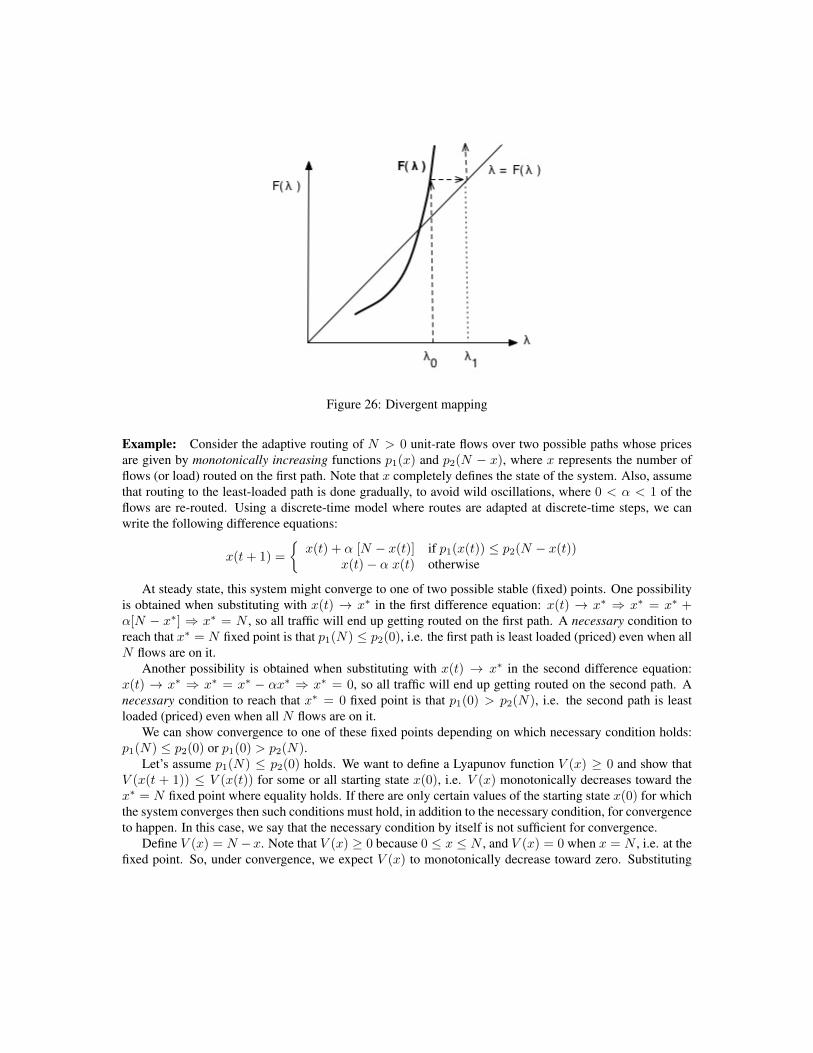
Figure 26: Divergent mapping

Example: Consider the adaptive routing of N > 0 unit-rate flows over two possible paths whose pricesare given by monotonically increasing functions p1(x) and p2(N − x), where x represents the number offlows (or load) routed on the first path. Note that x completely defines the state of the system. Also, assumethat routing to the least-loaded path is done gradually, to avoid wild oscillations, where 0 < α < 1 of theflows are re-routed. Using a discrete-time model where routes are adapted at discrete-time steps, we canwrite the following difference equations:

x(t+ 1) =

{x(t) + α [N − x(t)] if p1(x(t)) ≤ p2(N − x(t))

x(t)− α x(t) otherwise

At steady state, this system might converge to one of two possible stable (fixed) points. One possibilityis obtained when substituting with x(t) → x∗ in the first difference equation: x(t) → x∗ ⇒ x∗ = x∗ +α[N − x∗] ⇒ x∗ = N , so all traffic will end up getting routed on the first path. A necessary condition toreach that x∗ = N fixed point is that p1(N) ≤ p2(0), i.e. the first path is least loaded (priced) even when allN flows are on it.

Another possibility is obtained when substituting with x(t) → x∗ in the second difference equation:x(t) → x∗ ⇒ x∗ = x∗ − αx∗ ⇒ x∗ = 0, so all traffic will end up getting routed on the second path. Anecessary condition to reach that x∗ = 0 fixed point is that p1(0) > p2(N), i.e. the second path is leastloaded (priced) even when all N flows are on it.

We can show convergence to one of these fixed points depending on which necessary condition holds:p1(N) ≤ p2(0) or p1(0) > p2(N).

Let’s assume p1(N) ≤ p2(0) holds. We want to define a Lyapunov function V (x) ≥ 0 and show thatV (x(t + 1)) ≤ V (x(t)) for some or all starting state x(0), i.e. V (x) monotonically decreases toward thex∗ = N fixed point where equality holds. If there are only certain values of the starting state x(0) for whichthe system converges then such conditions must hold, in addition to the necessary condition, for convergenceto happen. In this case, we say that the necessary condition by itself is not sufficient for convergence.

Define V (x) = N −x. Note that V (x) ≥ 0 because 0 ≤ x ≤ N , and V (x) = 0 when x = N , i.e. at thefixed point. So, under convergence, we expect V (x) to monotonically decrease toward zero. Substituting

for x(t+ 1) in V (x), we obtain:

V (x(t+ 1)) = N − x(t+ 1)

Given the pricing functions are monotonically increasing with load, p1(N) ≤ p2(0) ⇒ p1(x(t)) ≤p2(N − x(t)), ∀x(t), and we can only use the first difference equation to substitute for x(t+ 1):

V (x(t+ 1)) = N − (x(t) + α[N − x(t)]) = (1− α)(N − x(t))

V (x(t+ 1)) = (1− α)V (x(t)) ≤ V (x(t))

So, we can conclude that the system is convergent regardless of the starting state x(0) as long as 0 < α < 1.Thus, 0 < α < 1, along with the necessary condition p1(N) ≤ p2(0), represent necessary and sufficient

conditions for convergence.A similar convergence proof can be obtained if on the other hand, the necessary condition p1(0) > p2(N)

holds. End Example.

7 Case Study: Class-based Scheduling of Elastic FlowsIn this and the following section, we consider the modeling and control-theoretic analysis of two trafficcontrol case studies. This first case study [17, 9] concerns the performance of elastic flows, i.e., rate-adaptiveflows similar to TCP. The goal is to investigate the effect of class-based scheduling that isolates elastic flowsinto two classes (service queues) based on different characteristics, for example based on their lifetime(transfer size), or burstiness of their arrivals/departures and sending rate (window) dynamics. We want toshow the benefits of isolation, in terms of better predictability and fairness, over traditional shared queueingsystems.

We formulate two control models. In the first model (Section 7.1), each flow controls its input traffic ratebased on the aggregate state of the network due to all N flows. In the second model (Section 7.2), each flow(or class of homogeneous flows) controls its rate based on its own individual state within the network. Weassume that the flows use PI control for adapting their sending rate.

In the aggregate control model, the packet sending rate of flow i, denoted by xi(t), is adapted based onthe difference between a target total buffer space, denoted by B, and the current total number of outstandingpackets, denoted by q(t). In the individual control model, xi(t) is adapted based on flow (or class) i’s target,denoted by Bi, and its current number of outstanding packets, denoted by qi(t). We denote by c(t) the totalpacket service rate, and by ci(t) the packet service rate of flow/class i. In what follows, for each controlmodel, we determine conditions under which the system stabilizes. We then solve for the values of thestate variables at equilibrium, and show whether fairness (or a form of weighted resource sharing) can beachieved. Table 3 lists all system variables along with their meanings.

7.1 Aggregate Control or SharingUnder aggregate PI control, the evolution of the system state is described by the following differentialequations:

xi(t) = αi(B − q(t))

q(t) =

N∑j=1

xj(t)− c(t) (15)

Table 3: Table defining system variablesVariable MeaningN total number of flows (or classes of homogeneous flows)xi(t) packet sending rate of flow/class iqi(t) number of outstanding packets of flow/class ici(t) packet service rate of flow/class iq(t) total number of outstanding packetsc(t) total packet service rateB target total buffer spaceBi target buffer space allocated to flow/class iαi parameter controlling increase and decrease rate of xi(t)

Stability Condition: Without loss of generality, assume a constant packet service rate (i.e. c(t) = C forall t), all flows start with the same initial input state (i.e. xi(0) is the same for all i), and that all flows adaptat the same rate (i.e. αi = α for all i). Then, Equations (15) can be re-written as:

xi(t) = α(B − q(t))

q(t) =

N∑j=1

xj(t)− C (16)

Since flows adapt their xi(t) at the same rate, then xi(t) =

∑N

j=1xj(t)

N for all i. Denote by e(t) the error attime t, i.e. e(t) = B − q(t), and let y(t) =

∑Nj=1 xj(t)− C. Equations (16) can then be re-written as:

y(t)

N= α e(t)

q(t) = y(t) (17)

Taking the Laplace transform of Equations (17), and assuming the buffer is initially empty (i.e. q(0) = 0),we get:

1

N(sY (s)− y(0)) = α E(s)

s Q(s) = Y (s)

E(s) = B −Q(s) (18)

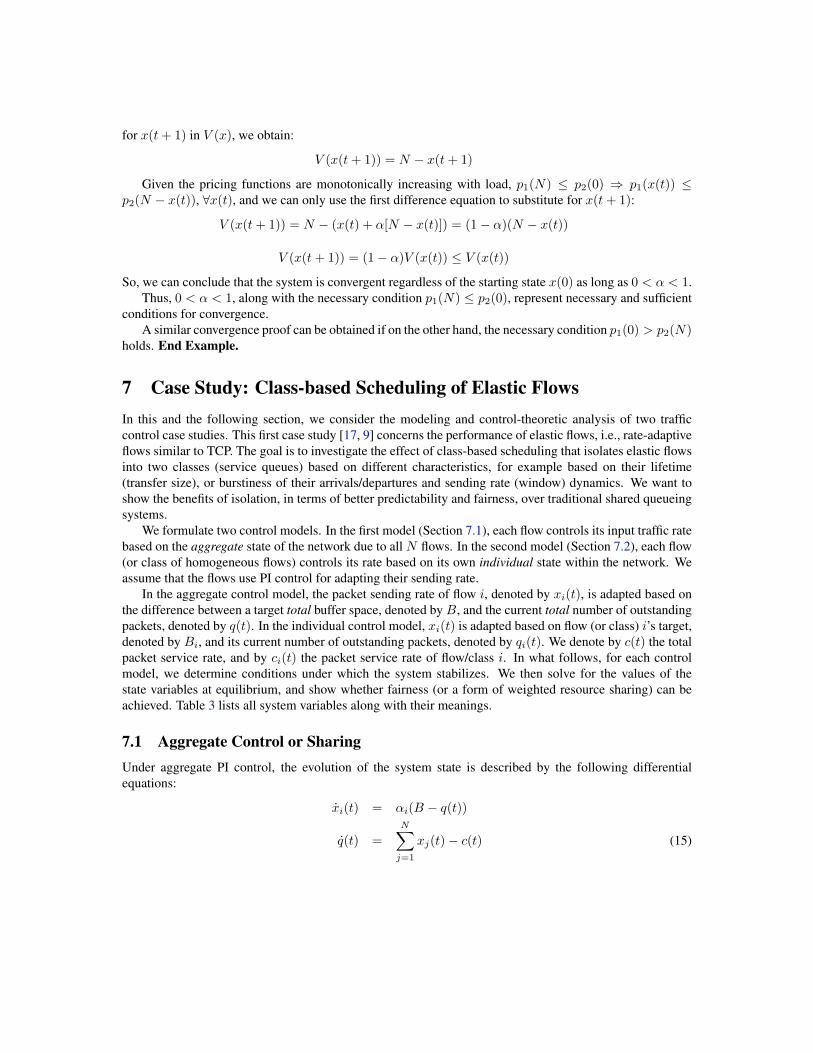
Solving Equations (18), we obtain the closed-loop system’s characteristic equation (see Figure 27 for thesystem’s block diagram):

s2 + α N = 0⇒ s =+− j√α N (19)

For α > 0, this system is marginally stable. However, the magnitude of oscillations increases for higherα and/or higher N .

This indicates that the existence of flows that rapidly change their sending rates through high values ofαi can cause the system to have high oscillations. This suggests that elastic flows that aggressively change

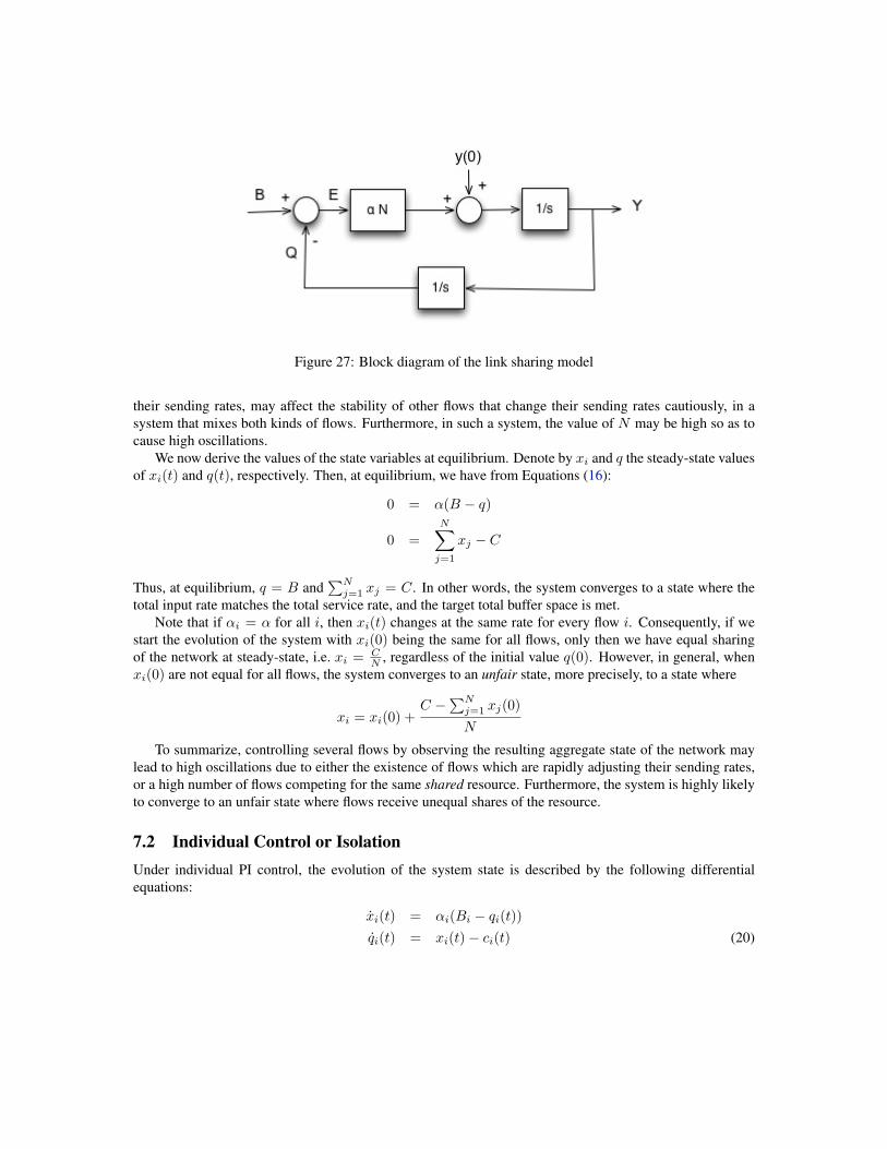
Figure 27: Block diagram of the link sharing model

their sending rates, may affect the stability of other flows that change their sending rates cautiously, in asystem that mixes both kinds of flows. Furthermore, in such a system, the value of N may be high so as tocause high oscillations.

We now derive the values of the state variables at equilibrium. Denote by xi and q the steady-state valuesof xi(t) and q(t), respectively. Then, at equilibrium, we have from Equations (16):

0 = α(B − q)

0 =

N∑j=1

xj − C

Thus, at equilibrium, q = B and∑Nj=1 xj = C. In other words, the system converges to a state where the

total input rate matches the total service rate, and the target total buffer space is met.Note that if αi = α for all i, then xi(t) changes at the same rate for every flow i. Consequently, if we

start the evolution of the system with xi(0) being the same for all flows, only then we have equal sharingof the network at steady-state, i.e. xi = C

N , regardless of the initial value q(0). However, in general, whenxi(0) are not equal for all flows, the system converges to an unfair state, more precisely, to a state where

xi = xi(0) +C −

∑Nj=1 xj(0)

N

To summarize, controlling several flows by observing the resulting aggregate state of the network maylead to high oscillations due to either the existence of flows which are rapidly adjusting their sending rates,or a high number of flows competing for the same shared resource. Furthermore, the system is highly likelyto converge to an unfair state where flows receive unequal shares of the resource.

7.2 Individual Control or IsolationUnder individual PI control, the evolution of the system state is described by the following differentialequations:

xi(t) = αi(Bi − qi(t))qi(t) = xi(t)− ci(t) (20)

Recall that under individual control, flow/class i regulates its input, xi(t), based on its own number ofoutstanding packets. For simplicity, assume a constant packet service rate, i.e. ci(t) = Ci for all t. Followingthe same stability analysis as aggregate control, it is easy to see that flow/class i stabilizes and the poles ofthe closed-loop system are:8

s =+− j√αi

Observe that, unlike aggregate control, flows/classes are isolated from each other. Therefore, the existence offlows/classes that rapidly change their sending rates through high values of αi, does not affect the stability ofother flows. This isolation can be implemented using, for example, a class-based queueing (CBQ) discipline[7]. In such CBQ system, each class of homogeneous flows can be allocated its own buffer space and servicecapacity.

We now derive the values of the state variables of flow/class i at equilibrium. Denote by xi and qi thesteady-state values of xi(t) and qi(t), respectively. Then, at equilibrium, we have from Equations (20):

0 = αi(Bi − qi)0 = xi − Ci

Thus, at equilibrium, qi = Bi and xi = Ci. In other words, each flow/class i converges to a state where itsinput rate matches its allocated service rate, and its target buffer space is met. We note that if the allocatedbuffers Bi and service capacities Ci are equal, then every flow receives an equal share of the resources, re-gardless of the initial values xi(0) and qi(0). One can also achieve a weighted resource sharing by assigningdifferent Bi and Ci allocations. Thus, a flow/class with higher priority (e.g., short interactive TCP flows op-erating aggressively in slow start) can be allocated more resources, so as to receive better throughput/delayservice than other flows (e.g., long TCP flows operating cautiously in congestion avoidance).

To summarize, controlling each flow (or class of homogeneous flows) by observing its own individualstate within the network provides isolation between them. Thus, stability can be achieved for a flow/classregardless of the behavior and number of other flows/classes. Furthermore, the system can converge to a fairstate where flows/classes receive a weighted share of the resources.

8 Case Study: Elastic Transport TunnelConsider n regular user connections between sending and receiving end-hosts, all passing through two “gate-ways” — let’s call them a source gateway and a destination gateway. Our main goal is to provide a “softbandwidth-guaranteed” tunnel [8] for these user flows over an Internet path of bottleneck capacity C, whichis also shared by another set of x flows, representing cross traffic (see Figure 28). By “soft” guarantee wemean that there is no explicit resource reservation. Consider that user and cross-traffic connections are allrate-adaptive connections (similar to TCP). These x cross-traffic connections present a challenge: as x keepschanging, the bandwidth allocation for the n user flows keeps changing in tandem. So an important questionis whether it is possible to “counter” the change in x so as to ensure that the n user flows are able to maintaina desirable bandwidth.

Clearly without the intervention of the two gateways, the answer to the above question is no. Whendifferent flows share a link, the effect of each individual flow (or an aggregate of flows) affects the rest sinceall are competing for a fixed amount of resources. However, if the gateways dynamically maintain a number

8 We set N = 1 in Equation (19).

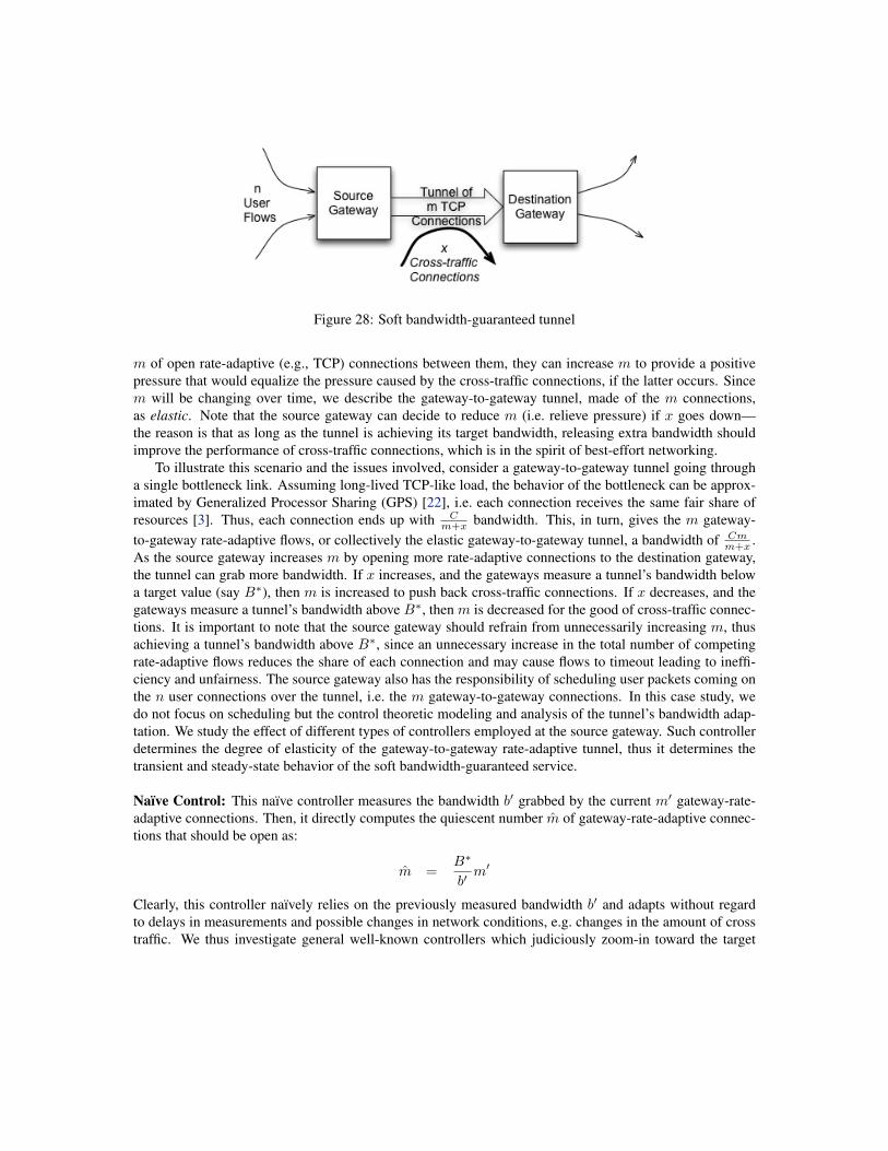
Figure 28: Soft bandwidth-guaranteed tunnel

m of open rate-adaptive (e.g., TCP) connections between them, they can increase m to provide a positivepressure that would equalize the pressure caused by the cross-traffic connections, if the latter occurs. Sincem will be changing over time, we describe the gateway-to-gateway tunnel, made of the m connections,as elastic. Note that the source gateway can decide to reduce m (i.e. relieve pressure) if x goes down—the reason is that as long as the tunnel is achieving its target bandwidth, releasing extra bandwidth shouldimprove the performance of cross-traffic connections, which is in the spirit of best-effort networking.

To illustrate this scenario and the issues involved, consider a gateway-to-gateway tunnel going througha single bottleneck link. Assuming long-lived TCP-like load, the behavior of the bottleneck can be approx-imated by Generalized Processor Sharing (GPS) [22], i.e. each connection receives the same fair share ofresources [3]. Thus, each connection ends up with C

m+x bandwidth. This, in turn, gives the m gateway-to-gateway rate-adaptive flows, or collectively the elastic gateway-to-gateway tunnel, a bandwidth of Cm

m+x .As the source gateway increases m by opening more rate-adaptive connections to the destination gateway,the tunnel can grab more bandwidth. If x increases, and the gateways measure a tunnel’s bandwidth belowa target value (say B∗), then m is increased to push back cross-traffic connections. If x decreases, and thegateways measure a tunnel’s bandwidth above B∗, then m is decreased for the good of cross-traffic connec-tions. It is important to note that the source gateway should refrain from unnecessarily increasing m, thusachieving a tunnel’s bandwidth above B∗, since an unnecessary increase in the total number of competingrate-adaptive flows reduces the share of each connection and may cause flows to timeout leading to ineffi-ciency and unfairness. The source gateway also has the responsibility of scheduling user packets coming onthe n user connections over the tunnel, i.e. the m gateway-to-gateway connections. In this case study, wedo not focus on scheduling but the control theoretic modeling and analysis of the tunnel’s bandwidth adap-tation. We study the effect of different types of controllers employed at the source gateway. Such controllerdetermines the degree of elasticity of the gateway-to-gateway rate-adaptive tunnel, thus it determines thetransient and steady-state behavior of the soft bandwidth-guaranteed service.

Naıve Control: This naıve controller measures the bandwidth b′ grabbed by the current m′ gateway-rate-adaptive connections. Then, it directly computes the quiescent number m of gateway-rate-adaptive connec-tions that should be open as:

m =B∗

b′m′

Clearly, this controller naıvely relies on the previously measured bandwidth b′ and adapts without regardto delays in measurements and possible changes in network conditions, e.g. changes in the amount of crosstraffic. We thus investigate general well-known controllers which judiciously zoom-in toward the target

bandwidth value. To that end, let us develop a flow-level model of the system dynamics. The change inthe bandwidth grabbed b(t) by the m(t) gateway-rate-adaptive flows (constituting the elastic gateway-to-gateway tunnel) can be described as:

b(t) = α[(C −B∗)m(t)−B∗x(t)]

This dynamic equation captures what we want to model: b(t) increases with m(t), and decreases as thenumber of cross-connections x(t) increases. α is a constant that represents the degree of multiplexing offlows and we choose it here to be the steady-state connection’s fair share ratio of the bottleneck capacity. Atsteady-state, b(t) equals zero, which yields (as expected):

B∗ =Cm

(x+ m)

where m and x represent the steady-state values for the number of gateway-rate-adaptive flows and cross-traffic flows, respectively. Based of the current bandwidth allocation b(t) and the target bandwidth B∗, anerror signal e(t) can be obtained as:

e(t) = B∗ − b(t)

P and PI Control: A controller would adjust m(t) based on the value of e(t). For a simple Proportionalcontroller (P-type), such adjustment is described by:

m(t) = Kpe(t) (21)

Recall that P-type controllers are known to result in a non-zero steady-state error. To exactly achieve thetarget B∗ (i.e. with zero steady-state error), a Proportional-Integral (PI-type) controller can be used:

m(t) = Kpe(t) +Ki

∫e(t) dt (22)

Figure 29 shows the block diagram of this elastic-tunnel model. In the Laplace domain, denoting the con-troller transfer function by Gc(s), the output B(s) is given by:

B(s) =Gc(s)G1(s)

1 +Gc(s)G1(s)B∗(s) +

G2(s)

1 +Gc(s)G1(s)X(s) (23)

where G1(s) is given by:

G1(s) =β

s

where β = α(C −B∗). G2(s) is given by:

G2(s) =γ

s

where γ = −αB∗. For the P-controller, from Equation (21), Gc(s) is simply Kp. For the PI-controller,from Equation (22), C(s) equals Kp + Ki

s . Thus, the transfer function B(s)B∗ in the presence of a P-controller

is given by:

B(s)

B∗=

Kpβ

s+Kpβ

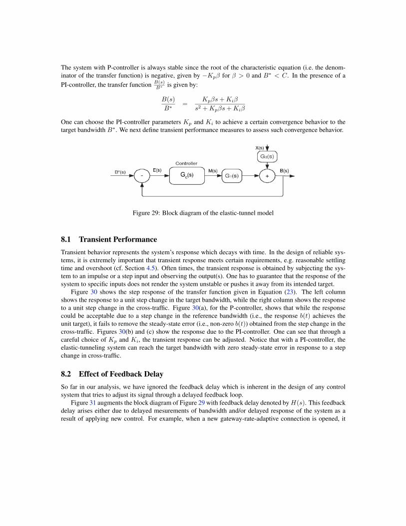
The system with P-controller is always stable since the root of the characteristic equation (i.e. the denom-inator of the transfer function) is negative, given by −Kpβ for β > 0 and B∗ < C. In the presence of aPI-controller, the transfer function B(s)

B∗ is given by:

B(s)

B∗=

Kpβs+Kiβ

s2 +Kpβs+Kiβ

One can choose the PI-controller parameters Kp and Ki to achieve a certain convergence behavior to thetarget bandwidth B∗. We next define transient performance measures to assess such convergence behavior.

Figure 29: Block diagram of the elastic-tunnel model

8.1 Transient PerformanceTransient behavior represents the system’s response which decays with time. In the design of reliable sys-tems, it is extremely important that transient response meets certain requirements, e.g. reasonable settlingtime and overshoot (cf. Section 4.5). Often times, the transient response is obtained by subjecting the sys-tem to an impulse or a step input and observing the output(s). One has to guarantee that the response of thesystem to specific inputs does not render the system unstable or pushes it away from its intended target.

Figure 30 shows the step response of the transfer function given in Equation (23). The left columnshows the response to a unit step change in the target bandwidth, while the right column shows the responseto a unit step change in the cross-traffic. Figure 30(a), for the P-controller, shows that while the responsecould be acceptable due to a step change in the reference bandwidth (i.e., the response b(t) achieves theunit target), it fails to remove the steady-state error (i.e., non-zero b(t)) obtained from the step change in thecross-traffic. Figures 30(b) and (c) show the response due to the PI-controller. One can see that through acareful choice of Kp and Ki, the transient response can be adjusted. Notice that with a PI-controller, theelastic-tunneling system can reach the target bandwidth with zero steady-state error in response to a stepchange in cross-traffic.

8.2 Effect of Feedback DelaySo far in our analysis, we have ignored the feedback delay which is inherent in the design of any controlsystem that tries to adjust its signal through a delayed feedback loop.

Figure 31 augments the block diagram of Figure 29 with feedback delay denoted byH(s). This feedbackdelay arises either due to delayed mesurements of bandwidth and/or delayed response of the system as aresult of applying new control. For example, when a new gateway-rate-adaptive connection is opened, it

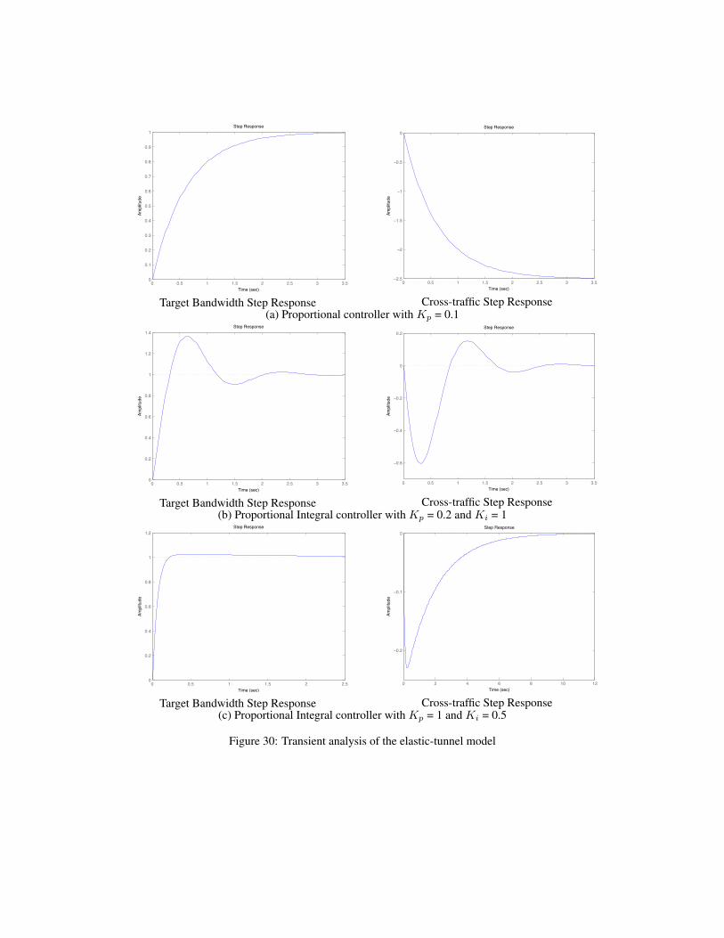
Step Response

Time (sec)

Ampl

itude

0 0.5 1 1.5 2 2.5 3 3.50

0.1

0.2

0.3

0.4

0.5

0.6

0.7

0.8

0.9

1

Target Bandwidth Step Response

Step Response

Time (sec)

Ampl

itude

0 0.5 1 1.5 2 2.5 3 3.52.5

2

1.5

1

0.5

0

Cross-traffic Step Response(a) Proportional controller with Kp = 0.1

Step Response

Time (sec)

Ampl

itude

0 0.5 1 1.5 2 2.5 3 3.50

0.2

0.4

0.6

0.8

1

1.2

1.4

Target Bandwidth Step Response

Step Response

Time (sec)

Ampl

itude

0 0.5 1 1.5 2 2.5 3 3.5

0.6

0.4

0.2

0

0.2

Cross-traffic Step Response(b) Proportional Integral controller with Kp = 0.2 and Ki = 1

Step Response

Time (sec)

Ampl

itude

0 0.5 1 1.5 2 2.50

0.2

0.4

0.6

0.8

1

1.2

Target Bandwidth Step Response

Step Response

Time (sec)

Ampl

itude

0 2 4 6 8 10 12

0.2

0.1

0

Cross-traffic Step Response(c) Proportional Integral controller with Kp = 1 and Ki = 0.5

Figure 30: Transient analysis of the elastic-tunnel model

Figure 31: Elastic-tunnel model (with feedback delay)

doesn’t get its steady-state throughput instantaneously, rather after some delay (say τ ). Thus, H(s) is givenby:

H(s) = e−τs

where τ represents the feedback time delay. For small τ , the above equation can be approximated by:

H(s) ≈ 1− τs

If we are using a PI-controller, the characteristic equation in the presence of feedback delay becomes:

s2(1− βτKp) + s(Kpβ − βτKi) + βKi = 0

Figure 32 shows the response of the PI-controller to a unit step change in the target bandwidth. As thefeedback delay τ increases, the system may not converge to the target bandwidth.

Step Response

Time (sec)

Ampl

itude

0 10 20 30 40 50 60 700

0.2

0.4

0.6

0.8

1

1.2

1.4

1.6

1.8

2

Target Bandwidth Step Response

Step Response

Time (sec)

Ampl

itude

0 5 10 15 20 25 30 35 40 45 500.5

0

0.5

1

1.5

2

2.5

Response with Feedback DelayProportional Integral controller with Kp = 0.01 and Ki = 0.02

Figure 32: Transient analysis of the elastic-tunnel model (with feedback delay)

9 Exercises1. Let r be a max-min fair rate vector corresponding to a given network and set of flows. This max-min

fair allocation maximizes the allocation of each flow i subject to the constraint that an incrementalincrease in i’s allocation does not cause a decrease in some other flow’s allocation that is already assmall as i’s or smaller.

(a) Suppose that some of the flows are eliminated and let r be a corresponding max-min fair ratevector. Show by example that we may have rp < rp for some of the remaining flows p.

(b) Suppose that some of the link capacities are increased and let r be a corresponding max-min fairrate vector. Show by example that we may have rp < rp for some flows p.

2. Consider two network links in tandem (one after the other) of capacities 6 Mbps each. For two differ-ent sets of elastic flows (i.e. the utility function of each flow/user is a log function of its allocated rate),you are asked to write down the corresponding network optimization problem, where the network triesto maximize the sum of flow utilities subject to link capacity constraints. For each set of flows, de-scribed in parts (a) and (b) below, rewrite the constrained optimization problem as an unconstrainedoptimization problem: write down the Lagrangian function and corresponding equations to solve forthe optimal rate allocation. What are the optimal rates allocated to different flows for each one of thesetwo settings?

(a) Consider two flows: one flow using the first link only and another flow using both links.

(b) Consider the same two flows from part (a), as well as a third flow using the second link only.

3. Consider two network links in tandem (one after the other) of capacities 6 Mbps each. Assume threeflows: one flow using the first link only, another flow using the second link only, and a third flow usingboth links. Assume the utility function of each flow/user is a log function of its allocated rate, and thatthe two-link flow is given a weight of 2, while the two one-link flows are given a weight of 1.

You are asked to write down the corresponding network optimization problem, where the networktries to maximize the sum of the weighted flow utilities subject to link capacity constraints. Rewritethe constrained optimization problem as an unconstrained optimization problem: write down the La-grangian function and corresponding equations to solve for the optimal rate allocation. What are theoptimal rates allocated to each flow?

4. Consider a source adapting its sending rate x(t) so the buffer size of its path’s bottleneck b(t) staysat a certain target value T . Denote the error signal by e(t) = T − b(t). The sending rate is adaptedaccording to one of the following three controllers:

(a) x(t) = Kpe(t)

(b) x(t) = Kpe(t) +Ki

∫ t0e(t)dt

(c) x(t) = Kpe(t) +Ki

∫ t0e(t)dt+Kd

ddte(t)

where Kp,Ki,Kd are constant parameters of the rate controllers.

(a) Assume c(t) is the capacity available to the source at time t, write down the differential equationfor b(t).

(b) By transforming the system to the Laplace domain, determine the conditions under which thesystem is stable for each type of controller, i.e. does b(t) converge to a given T for certainvalues of Kp,Ki,Kd. Do this by examining the roots (poles) of the characteristic equation ofthe system’s transfer function. Draw the block diagram of the system that shows the relationshipsbetween the system variables in the (Laplace) s-domain for each type of controller.

(c) Again by examining the roots (poles) of the characteristic equation of the system’s transfer func-tion and using the Final Value Theorem, compare the transient and steady-state performanceunder each type of controller.

(d) Support your answers above by numerically solving the system’s equations over time for eachtype of controller. Assume a small time step ∆, say ∆ = 1, and solve the discretized versionof the equations at these time steps – you can then approximate the differentiation d

dtb(t) byb(t)− b(t− 1).

5. Consider an adaptation of a transmission window w whose goal is to reach a target window T asfollows:

w(k+1) = wk + α(T − wk)

where 0 < α < 1.

(a) Derive the necessary condition (if any) for convergence to the target window size.

(b) Use the Lyapunov method to show whether the system converges regardless of the initial windowsize.

6. Given a system with the following adaptation rules: x(t), representing a sending rate, is adapted usingan AIMD policy, whereas p(t), representing the price, is adapted in proportion to how far x(t) is froma target capacity c:

dx(t)

dt= 1− x(t)p(x(t))

p(x(t)) = α(x(t)− c)

(a) Why is that system non-linear?

(b) Linearize the system around a certain operating point x0.

(c) By transforming the linearized system to the Laplace domain, obtain the condition on x0 underwhich the linearized system is stable.

7. This question is based on the paper The Revised ARPANET Routing Metric, by Zinky and Khanna[14]. A unified way to model adaptive resource management—whether it is TCP adaptive to REDor routing adaptive to changing link costs or other examples—is through two functions: a feedback(pricing) function such as that of RED or link utilization metric, and an adaptation function such asthat of TCP or utilization-based routing. Consider a resource that generates prices p and users thatadapt their load λ based on the currently reported p. Assume the following pricing and load adaptationfunctions:

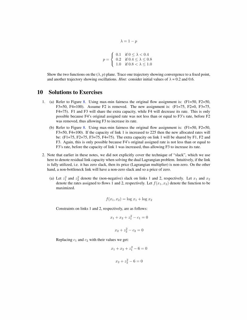
λ = 1− p

p =

0.1 if 0 ≤ λ < 0.40.2 if 0.4 ≤ λ ≤ 0.81.0 if 0.8 < λ ≤ 1.0

Show the two functions on the (λ, p) plane. Trace one trajectory showing convergence to a fixed point,and another trajectory showing oscillations. Hint: consider initial values of λ = 0.2 and 0.6.

10 Solutions to Exercises1. (a) Refer to Figure 8. Using max-min fairness the original flow assignment is: (F1=50, F2=50,

F3=50, F4=100). Assume F2 is removed. The new assignment is: (F1=75, F2=0, F3=75,F4=75). F1 and F3 will share the extra capacity, while F4 will decrease its rate. This is onlypossible because F4’s original assigned rate was not less than or equal to F3’s rate, before F2was removed, thus allowing F3 to increase its rate.

(b) Refer to Figure 8. Using max-min fairness the original flow assignment is: (F1=50, F2=50,F3=50, F4=100). If the capacity of link 1 is increased to 225 then the new allocated rates willbe: (F1=75, F2=75, F3=75, F4=75). The extra capacity on link 1 will be shared by F1, F2 andF3. Again, this is only possible because F4’s original assigned rate is not less than or equal toF3’s rate, before the capacity of link 1 was increased, thus allowing F3 to increase its rate.

2. Note that earlier in these notes, we did not explicitly cover the technique of “slack”, which we usehere to denote residual link capacity when solving the dual Lagrangian problem. Intuitively, if the linkis fully utilized, i.e. it has zero slack, then its price (Lagrangian multiplier) is non-zero. On the otherhand, a non-bottleneck link will have a non-zero slack and so a price of zero.

(a) Let z21 and z2

2 denote the (non-negative) slack on links 1 and 2, respectively. Let x1 and x2

denote the rates assigned to flows 1 and 2, respectively. Let f(x1, x2) denote the function to bemaximized.

f(x1, x2) = log x1 + log x2

Constraints on links 1 and 2, respectively, are as follows:

x1 + x2 + z21 − c1 = 0

x2 + z22 − c2 = 0

Replacing c1 and c2 with their values we get:

x1 + x2 + z21 − 6 = 0

x2 + z22 − 6 = 0

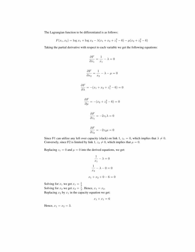
The Lagrangian function to be differentiated is as follows:

F (x1, x2) = log x1 + log x2 − λ(x1 + x2 + z21 − 6)− µ(x2 + z2

2 − 6)

Taking the partial derivative with respect to each variable we get the following equations:

∂F

∂x1=

1

x1− λ = 0

∂F

∂x2=

1

x2− λ− µ = 0

∂F

∂λ= −(x1 + x2 + z2

1 − 6) = 0

∂F

∂µ= −(x2 + z2

2 − 6) = 0

∂F

∂z1= −2z1λ = 0

∂F

∂z2= −2z2µ = 0

Since F1 can utilize any left over capacity (slack) on link 1, z1 = 0, which implies that λ 6= 0.Conversely, since F2 is limited by link 1, z2 6= 0, which implies that µ = 0.

Replacing z1 = 0 and µ = 0 into the derived equations, we get:

1

x1− λ = 0

1

x2− λ− 0 = 0

x1 + x2 + 0− 6 = 0

Solving for x1 we get x1 = 1λ

Solving for x2 we get x2 = 1λ . Hence, x1 = x2.

Replacing x2 by x1 in the capacity equation we get:

x1 + x1 = 6

Hence, x1 = x2 = 3.

(b) Let z21 and z2

2 denote the slack on links 1 and 2, respectively. Let x1, x2 and x3 denote the ratesassigned to flows 1, 2 and 3, respectively. Let f(x1, x2, x3) denote the function to be maximized.

f(x1, x2, x3) = log x1 + log x2 + log x3

Constraints on links 1 and 2, respectively, are as follows:

x1 + x2 + z21 − c1 = 0

x3 + x2 + z22 − c2 = 0

Replacing c1 and c2 with their values we get:

x1 + x2 + z21 − 6 = 0

x3 + x2 + z22 − 6 = 0

The Lagrangian function to be differentiated is as follows:

F (x1, x2, x3) = log x1 + log x2 + log x3 − λ(x1 + x2 + z21 − 6)− µ(x3 + x2 + z2

2 − 6)

Taking the partial derivative with respect to each variable we get the following equations:

∂F

∂x1=

1

x1− λ = 0

∂F

∂x2=

1

x2− λ− µ = 0

∂F

∂x3=

1

x3− µ = 0

∂F

∂λ= −(x1 + x2 + z2

1 − 6) = 0

∂F

∂µ= −(x3 + x2 + z2

2 − 6) = 0

∂F

∂z1= −2z1λ = 0

∂F

∂z2= −2z2µ = 0

From the equations above we can deduce the following:

x1 =1

λ

x2 =1

λ+ µ

x3 =1

µ

Since F1 and F3 can utilize any left over capacity (slack) on links 1 and 2, z1 = z2 = 0. Thisimplies that λ 6= 0 and µ 6= 0.

Replacing z1 = 0 and z2 = 0 into the derived equations we get:

x1 + x2 = 6

x2 + x3 = 6

Replacing x1 by 1λ , x2 by 1

λ+µ and x3 by 1µ into the equations above, we get:

1

λ+

1

λ+ µ= 6

1

λ+ µ+

1

µ= 6

Multiplying the first equation by (-1) and adding it to second equation, results in the following:

1

µ− 1

λ= 0

Hence, λ = µ

Thus, x1 = x3 = 1λ and x2 = 1

2λ = x1

2 = x3

2

Finally we get:

x1 +x1

2= 6

Hence, x1 = x3 = 4 and x2 = 2.

3. The objective function we want to maximize is:

F (x) = log x1 + log x2 + 2 log x3

subject to the capacity constraints:

x1 + x3 ≤ 6x2 + x3 ≤ 6x1, x2, x3 ≥ 0

The Lagrangian (unconstrained) function that we want to maximize is:

L(x) = log x1 + log x2 + 2 log x3 − λ1(x1 + x3 − 6)− λ2(x2 + x3 − 6)

Note that we do not explicitly include the slacks for the link capacities here, since both links shouldbe fully utilized as the one-link flows are not limited by any other link, so the slack values are zero.

Taking the partial derivatives of L(.) we obtain:∂L∂x1

= 1x1− λ1 = 0⇒ x1 = 1

λ1

∂L∂x2

= 1x2− λ2 = 0⇒ x2 = 1

λ2

∂L∂x3

= 2x3− (λ1 + λ2) = 0⇒ x3 = 2

λ1+λ2

∂L∂λ1

= 0⇒ x1 + x3 − 6 = 0⇒ x1 + x3 = 6

∂L∂λ2

= 0⇒ x2 + x3 − 6 = 0⇒ x2 + x3 = 6

The last two equations yield x1 = x2 ⇒ λ1 = λ2 = λ

From the capacity equation, we have:

x1 + x3 = 1λ + 2

2λ = 6⇒ λ = 13 , thus

x1 = x2 = 3, and x3 = 6− 3 = 3.

4. We use the following notation:

In the time domain we have:b(t), buffer size at time tx(t), sending rate at time tc(t), service rate at time tT , target buffer sizee(t), error (difference between current buffer size and the target) at time t

In the frequency domain we have:B(s), current buffer sizeX(s), sending rateC(s), service rateT (s), target buffer sizeE(s), error signalD(s), controller (based on error signal computes sending rate)

We will assume that the target buffer size and the buffer’s service rate are constant values.

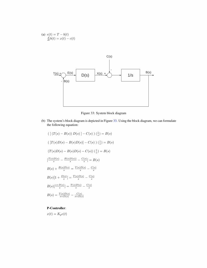
(a) e(t) = T − b(t)ddtb(t) = x(t)− c(t)

D(s) 1/s

C(s)

X(s) + B(s)

- B(s)

T(s) + E(s)-

Figure 33: System block diagram

(b) The system’s block diagram is depicted in Figure 33. Using the block diagram, we can formulatethe following equation:

( [ (T (s)−B(s)) D(s) ]− C(s) ) ( 1s ) = B(s)

( [T (s)D(s)−B(s)D(s)]− C(s) ) ( 1s ) = B(s)

(T (s)D(s)−B(s)D(s)− C(s)) ( 1s ) = B(s)

[T (s)D(s)s − B(s)D(s))

s − C(s)s ] = B(s)

B(s) + B(s)D(s)s = T (s)D(s)

s − C(s)s

B(s)[1 + D(s)s ] = T (s)D(s)

s − C(s)s

B(s)[ s+D(s)s ] = T (s)D(s)

s − C(s)s

B(s) = T (s)D(s)s+D(s) −

C(s)s+D(s)

P-Controller:

x(t) = Kpe(t)

By taking the Laplace transform we get:

X(s) = KpE(s)⇒ D(s) = X(s)E(s) = Kp

Replacing D(s) into the equation for B(s) we get:

B(s) =T (s)Kp

s+Kp− C(s)

s+Kp

Roots of the system’s characteristic equation are:

s+Kp = 0⇒ s = −Kp < 0Thus, system is stable for all values of Kp > 0

PI-Controller:

x(t) = Kpe(t) +Ki

∫ t0e(t)dt

By taking the Laplace transform we get:

X(s) = KpE(s) + Ki

s E(s)⇒ D(s) = X(s)E(s) = Kp + Ki

s

Replacing D(s) into the equation for B(s) we get:

B(s) =(Kp+

Kis )T (s)

s+(Kp+Kis )− C(s)

s+(Kp+Kis )

Roots of the system’s characteristic equation are:

s+Kp + Ki

s = 0s2 +Kps+Ki = 0a = 1, b = Kp, c = Ki

∆ = b2 − 4ac = K2p − 4(1)(Ki) = K2

p − 4Ki

s = −b±√

∆2a

s =−Kp±

√K2

p−4Ki

2

s = − 12Kp ± 1

2

√K2p − 4Ki

System will be stable with two real roots (i.e., overdamped) if the following conditions are true:Kp > 0K2p − 4Ki > 0⇒ K2

p > 4Ki√K2p − 4Ki < Kp ⇒ K2

p − 4Ki < K2p ⇒ Ki > 0

System will be stable with two complex roots (i.e., underdamped) if the following conditions aretrue:Kp > 0K2p − 4Ki < 0⇒ K2

p < 4Ki

PID-Controller:

x(t) = Kpe(t) +Ki

∫ t0e(t)dt+Kd

ddte(t)

By taking the Laplace transform we get:

X(s) = KpE(s) + Ki

s E(s) +KdsE(s)⇒ D(s) = X(s)E(s) = Kp + Ki

s +Kds

Replacing D(s) into the equation for B(s) we get:

B(s) =(Kp+

Kis +Kds)T (s)

s+(Kp+Kis +Kds)

− C(s)

s+(Kp+Kis +Kds)

Roots of the system’s characteristic equation are:

s+Kp + Ki

s +Kds = 0s2 +Kps+Ki +Kds

2 = 0(1 +Kd)s

2 +Kps+Ki = 0a = 1 +Kd, b = Kp, c = Ki

∆ = b2 − 4ac = K2p − 4(1 +Kd)(Ki) = K2

p − 4Ki(1 +Kd)

s = −b±√

∆2a

s =−Kp±

√K2

p−4Ki(1+Kd)

2(1+Kd)

s = − Kp

2(1+Kd) ±1

2(1+Kd)

√K2p − 4Ki(1 +Kd)

System will be stable with two real roots if the following conditions are true:Kp

1+Kd> 0

K2p − 4Ki(1 +Kd) > 0⇒ K2

p > 4Ki(1 +Kd)√K2p − 4Ki(1 +Kd) < Kp ⇒ K2

p − 4Ki(1 +Kd) < K2p ⇒ 4Ki(1 +Kd) > 0

System will be stable with two complex roots if the following conditions are true:Kp

1+Kd> 0

K2p − 4Ki(1 +Kd) < 0⇒ K2

p < 4Ki(1 +Kd)

(c) Final Value Theoremlimt→∞ f(t) = lims→0 sF (s)

Thus, we have:limt→∞ b(t) = lims→0 sB(s)

Note that,B(s) = T (s)D(s)

s+D(s) −C(s)s+D(s)

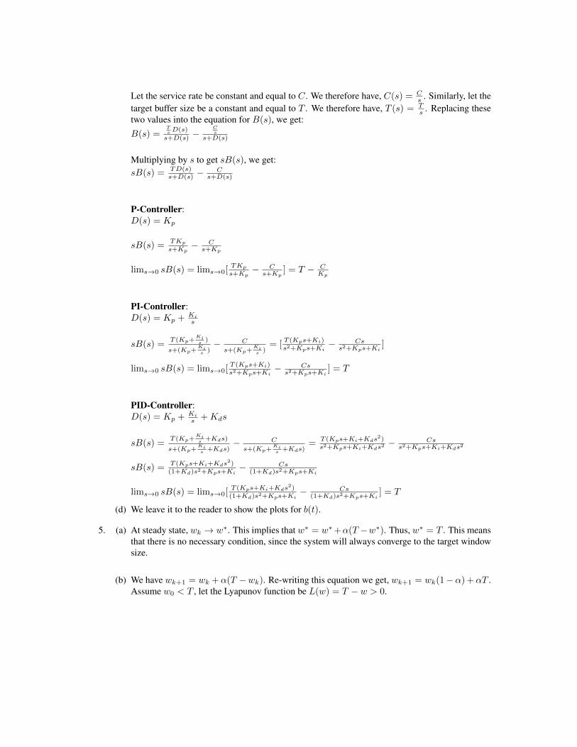
Let the service rate be constant and equal to C. We therefore have, C(s) = Cs . Similarly, let the

target buffer size be a constant and equal to T . We therefore have, T (s) = Ts . Replacing these

two values into the equation for B(s), we get:

B(s) =Ts D(s)

s+D(s) −Cs

s+D(s)

Multiplying by s to get sB(s), we get:sB(s) = TD(s)

s+D(s) −C

s+D(s)

P-Controller:D(s) = Kp

sB(s) =TKp

s+Kp− C

s+Kp

lims→0 sB(s) = lims→0[TKp

s+Kp− C

s+Kp] = T − C

Kp

PI-Controller:D(s) = Kp + Ki

s

sB(s) =T (Kp+

Kis )

s+(Kp+Kis )− C

s+(Kp+Kis )

= [T (Kps+Ki)s2+Kps+Ki

− Css2+Kps+Ki

]

lims→0 sB(s) = lims→0[T (Kps+Ki)s2+Kps+Ki

− Css2+Kps+Ki

] = T

PID-Controller:D(s) = Kp + Ki

s +Kds

sB(s) =T (Kp+

Kis +Kds)

s+(Kp+Kis +Kds)

− C

s+(Kp+Kis +Kds)

=T (Kps+Ki+Kds

2)s2+Kps+Ki+Kds2

− Css2+Kps+Ki+Kds2

sB(s) =T (Kps+Ki+Kds

2)(1+Kd)s2+Kps+Ki

− Cs(1+Kd)s2+Kps+Ki

lims→0 sB(s) = lims→0[T (Kps+Ki+Kds

2)(1+Kd)s2+Kps+Ki

− Cs(1+Kd)s2+Kps+Ki

] = T

(d) We leave it to the reader to show the plots for b(t).

5. (a) At steady state, wk → w∗. This implies that w∗ = w∗+α(T −w∗). Thus, w∗ = T . This meansthat there is no necessary condition, since the system will always converge to the target windowsize.

(b) We have wk+1 = wk +α(T −wk). Re-writing this equation we get, wk+1 = wk(1−α) +αT .Assume w0 < T , let the Lyapunov function be L(w) = T − w > 0.

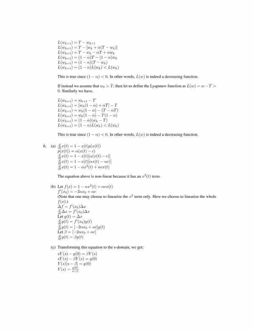
L(wk+1) = T − wk+1

L(wk+1) = T − [wk + α(T − wk)]L(wk+1) = T − wk − αT + αwkL(wk+1) = (1− α)T − (1− α)wkL(wk+1) = (1− α)(T − wk)L(wk+1) = (1− α)L(wk) < L(wk)

This is true since (1− α) < 0. In other words, L(w) is indeed a decreasing function.

If instead we assume that w0 > T , then let us define the Lyapunov function as L(w) = w−T >0. Similarly we have,

L(wk+1) = wk+1 − TL(wk+1) = [wk(1− α) + αT ]− TL(wk+1) = wk(1− α)− (T − αT )L(wk+1) = wk(1− α)− T (1− α)L(wk+1) = (1− α)(wk − T )L(wk+1) = (1− α)L(wk) < L(wk)

This is true since (1− α) < 0. In other words, L(w) is indeed a decreasing function.

6. (a) ddtx(t) = 1− x(t)p(x(t))p(x(t)) = α(x(t)− c)ddtx(t) = 1− x(t)[α(x(t)− c)]ddtx(t) = 1− x(t)[αx(t)− αc)]ddtx(t) = 1− αx2(t) + αcx(t)

The equation above is non-linear because it has an x2(t) term.

(b) Let f(x) = 1− αx2(t) + αcx(t)f ′(x0) = −2αx0 + αc(Note that one may choose to linearize the x2 term only. Here we choose to linearize the wholef(x).)∆f = f ′(x0)∆xddt∆x = f ′(x0)∆xLet y(t) = ∆xddty(t) = f ′(x0)y(t)ddty(t) = [−2αx0 + αc]y(t)Let β = [−2αx0 + αc]ddty(t) = βy(t)

(c) Transforming this equation to the s-domain, we get:

sY (s)− y(0) = βY (s)sY (s)− βY (s) = y(0)Y (s)[s− β] = y(0)

Y (s) = y(0)s−β

The root of the characteristic equation s − β is s = β. For the system to be stable, β must beless than zero. Assuming α > 0, we need the following to be true:

β < 0−2αx0 + αc < 0−2αx0 < −αc2αx0 > αcx0 >

c2

7. We leave it to the reader to produce the plot. Notice that the fixed point is (λ = 0.8, p = 0.2) wherethe pricing curve and the load curve intersect. Also the system diverges for starting λ = 0.2, whereasit converges for λ = 0.6. Specifically, in the latter case, λ = 0.6 yields p = 0.2, which in turn yieldsλ = 1− p = 0.8 and the system stabilizes at the fixed point.

References[1] ARCHIVE, I. http://archive.org/web/web.php. [Online; accessed June-11-2013].

[2] ATHURALIYA, S., LOW, S. H., LI, V. H., AND YIN, Q. REM: Active Queue Management. Netwrk.Mag. of Global Internetwkg. 15, 3 (May 2001), 48–53.

[3] CHIU, D.-M., AND JAIN, R. Analysis of the Increase and Decrease Algorithms for Congestion Avoid-ance in Computer Networks. Comput. Netw. ISDN Syst. 17, 1 (June 1989), 1–14.

[4] ETFORECASTS. http://www.etforecasts.com/. [Online; accessed June-11-2013].

[5] FALL, K., AND FLOYD, S. Simulation-based Comparisons of Tahoe, Reno and SACK TCP. SIG-COMM Comput. Commun. Rev. 26, 3 (July 1996), 5–21.

[6] FLOYD, S., AND JACOBSON, V. Random Early Detection Gateways for Congestion Avoidance.IEEE/ACM Trans. Netw. 1, 4 (Aug. 1993), 397–413.

[7] FLOYD, S., AND JACOBSON, V. Link-sharing and Resource Management Models for Packet Net-works. IEEE/ACM Trans. Netw. 3, 4 (Aug. 1995), 365–386.

[8] GUIRGUIS, M., BESTAVROS, A., MATTA, I., RIGA, N., DIAMANT, G., AND ZHANG, Y. ProvidingSoft Bandwidth Guarantees Using Elastic TCP-based Tunnels. In Proceedings of ISCC ’2004: TheNinth IEEE Symposium on Computers and Communications (Alexandria, Egypt, June 2004).

[9] GUO, L., AND MATTA, I. The War between Mice and Elephants. In Proceedings of ICNP’2001: The9th IEEE International Conference on Network Protocols (Riverside, CA, November 2001).

[10] HOLLOT, C., MISRA, V., TOWSLEY, D., AND GONG, W.-B. On Designing Improved Controllersfor AQM Routers Supporting TCP Flows. In INFOCOM 2001. Twentieth Annual Joint Conference ofthe IEEE Computer and Communications Societies. Proceedings. IEEE (2001), vol. 3, pp. 1726–1734vol.3.

[11] JACOBSON, V. Congestion Avoidance and Control. In Proc. ACM SIGCOMM (Stanford, CA, August1988).

[12] KELLY, F. Mathematical Modelling of the Internet. In Mathematics Unlimited - 2001 and Beyond.Springer-Verlag, 2001, pp. 685–702.

[13] KESHAV, S. Mathematical Foundations of Computer Networking. Addison-Wesley, 2012.

[14] KHANNA, A., AND ZINKY, J. The Revised ARPANET Routing Metric. In Symposium proceedingson Communications architectures & protocols (New York, NY, USA, 1989), SIGCOMM ’89, ACM,pp. 45–56.

[15] LAWRENCE S. BRAKMO AND LARRY L. PETERSON. TCP Vegas: End to End Congestion Avoidanceon a Global Internet. IEEE Journal on Selected Areas in Communications 13, 8 (1995), 1465–1480.

[16] LU, C. Feedback Control Theory: A Computer System’s Perspective. http://www.cs.virginia.edu/˜cl7v/cs851-talks/control_tutorial.ppt, 2001. [Online; accessedJune-11-2013].

[17] MATTA, I., AND GUO, L. Differentiated Predictive Fair Service for TCP Flows. In Proceedings ofICNP’2000: The 8th IEEE International Conference on Network Protocols (Osaka, Japan, October2000).

[18] MO, J., AND WALRAND, J. Fair End-to-end Window-based Congestion Control. IEEE/ACM Trans.Netw. 8, 5 (Oct. 2000), 556–567.

[19] NETCRAFT. http://www.netcraft.com/. [Online; accessed June-11-2013].

[20] OGATA, K. Modern Control Engineering. Prentice Hall, 2010.

[21] PADHYE, J., FIROIU, V., TOWSLEY, D. F., AND KUROSE, J. F. Modeling TCP Reno Performance:a Simple Model and its Empirical Validation. IEEE/ACM Trans. Netw. 8, 2 (Apr. 2000), 133–145.

[22] PAREKH, A. K., AND GALLAGHER, R. G. A Generalized Processor Sharing Approach to FlowControl in Integrated Services Networks: the Multiple Node Case. IEEE/ACM Trans. Netw. 2, 2 (Apr.1994), 137–150.

[23] SHENKER, S. Fundamental Design Issues for the Future Internet. IEEE J.Sel. A. Commun. 13, 7 (Sept.2006), 1176–1188.

[24] SRIKANT, R. The Mathematics of Internet Congestion Control. Birkhauser, 2004.

[25] WEI, D. X., JIN, C., LOW, S. H., AND HEGDE, S. FAST TCP: Motivation, Architecture, Algorithms,Performance. IEEE/ACM Trans. Netw. 14, 6 (Dec. 2006), 1246–1259.