Optimized Time-Dependent Congestion Pricing System for Large Networks:

Integrating Distributed Optimization, Departure Time Choice, and Dynamic

Traffic Assignment in the Greater Toronto Area

By

Aya Tollah Moustafa S. M. Aboudina

A thesis submitted in conformity with the requirements

for the degree of Doctor of Philosophy

Department of Civil Engineering

University of Toronto

© Copyright by Aya Aboudina, 2016

ii

Optimized Time-Dependent Congestion Pricing System for Large Networks:

Integrating Distributed Optimization, Departure Time Choice, and Dynamic

Traffic Assignment in the Greater Toronto Area

Aya Aboudina

Doctor of Philosophy

Department of Civil Engineering

University of Toronto

2016

Abstract

Congestion pricing is one of the most widely contemplated methods to manage traffic

congestion. The purpose of congestion pricing is to manage traffic demand generation and

supply allocation by charging fees (i.e., tolling) for the use of certain roads in order to distribute

traffic demand more evenly over time and space. This study presents a system for large-scale

optimal time-varying congestion pricing policy determination and evaluation. The proposed

system integrates a theoretical model of dynamic congestion pricing, a distributed optimization

algorithm, a departure time choice model, and a dynamic traffic assignment (DTA) simulation

platform, creating a unified optimal (location- and time-specific) congestion pricing system. The

system determines and evaluates the impact of optimal tolling on road traffic congestion (supply

side) and travellers’ behavioural choices, including departure time and route choices (demand

side). For the system’s large-scale nature and the consequent computational challenges, the

optimization algorithm is executed concurrently on a parallel cluster. The system is applied to

simulation-based case studies of tolling major highways in the Greater Toronto Area (GTA)

while capturing the regional effects of tolling. The models are developed and calibrated using

regional household travel survey data that reflect travellers’ heterogeneity. The DTA model is

calibrated using actual traffic counts from the Ontario Ministry of Transportation and the City of

Toronto. The main results indicate that: (1) more benefits are attained from variable tolling due

to departure time rescheduling as opposed to mostly re-routing only in the case of flat tolling, (2)

widespread spatial and temporal re-distributions of traffic are observed across the regional

network in response to tolling significant – yet limited – highways in the region, (3) optimal

iii

variable pricing mirrors congestion patterns and induces departure time re-scheduling and

rerouting patterns, resulting in improved average travel times and schedule delays at all scales,

(4) tolled routes have different sensitivities to identical toll changes, (5) the start times of longer

trips are more sensitive (elastic) to variable distance-based tolling policies compared to shorter

trips, (6) optimal tolls intended to manage traffic demand are significantly lower than those

intended to maximize toll revenues, (7) toll payers benefit from tolling even before toll revenues

are spent, and (8) the optimal tolling policies determined offer a win-win solution in which travel

times are improved while also raising funds to invest in sustainable transportation infrastructure.

iv

Acknowledgment

Alhamdulillah, all praise is due to Allah, the most gracious and the most merciful, for providing

me this opportunity, showering me with his countless blessings, and enabling me to finish my

PhD thesis.

First I would like to express my deep gratitude to my thesis supervisor Professor Baher Abdulhai

for his guidance, trust, patience, respect, and continuous support during the whole period of my

study. I would like also to extend my gratitude to Dr Hossam Abdelgawad for his sincere

guidance, support, and continuous help during my PhD journey that went beyond the research

related matters. Dr Hossam, I cannot thank you enough for your moral and intellectual support

and for all your help and valuable advices during the past six years. Special thanks go to

Professor Khandker M. Nurul Habib for his guidance in the departure time choice module and

his continuous support throughout the period of my study.

In addition, my sincere thanks go to the other members of my internal examination committee,

Professors Mathew Roorda and Amer Shalaby, for their valuable comments and suggestions and

for providing constructive feedback on my thesis. Special thanks go to my external examiner,

Professor Robin Lindsey from the University of British Columbia, for spending his time reading

my thesis, providing constructive feedback, and attending my final oral examination.

I would also acknowledge the generous financial support I received from the University of

Toronto, Professor Baher Abdulhai, Heavy Construction Association of Toronto (HCAT), and

Transportation Association of Canada (TAC).

My beloved parents, Dr Moustafa Aboudina and Dr Faiza Hemeida: thank you for your endless

love, prayers, continuous support and encouragement throughout my life, and for raising me up

to this point. This thesis would not have been possible without your continued motivation and

follow-up during the ups and downs of my PhD journey. Also I am deeply grateful to my dear

brother and role model, Dr Mohamed, and my lovely sisters, Radwa and Nashwa, for their love,

care, and constant encouragement. I would like also to express my deep gratitude and respect to

my brother-in-law, Dr Ahmed Awadallah, for simply being a true brother to me. Radwa and

Ahmed, the kindness and warmth I felt during my visits to you in the last six years made me feel

v

welcome, wanted, and content; thank you for always being there for me. A special mention goes

to my joyful and lovely niece and nephews, Haya, Yasseen, Yehia, and Omar, for filling my

heart with happiness and bringing a big smile on my face when seeing them or hearing their

news.

Thanks also extend to my former and current colleagues in the Transportation Group; most

remarkably, Samah El-Tantawy, Toka Muhammad, Sarah Salem, Mohamed Elshenawy, Islam

Kamel, Tamer Abdulazim, Bryce Sharman, Kasra Rezaee, Sami Hasnine, and Wafic El-Assi.

Samah El-Tantawy, it is hard to find words to express my gratitude to your endless support and

encouragement since we have known each other more than ten years ago; thank you for being a

close and lovely friend, a role model, and for never letting me down. Toka Muhammad, it was a

blessing having you as a colleague, a roommate for more than five years, and a forever sincere

friend; thank you for all your kindness, caring, patience to listen to my complaints when

struggling in my research, and for the valuable life lessons I have learned from you. Sarah

Salem, I have always admired and respected your positive attitude of maintaining a good spirit in

the most stressful moments. Islam Kamel, thank you for your support and help in the GTA

simulation model and the distributed computing part. Mohamed Elshenawy, I deeply appreciate

your valuable time and support in the distributed computing part. Second, and most importantly,

thank you for your continuous encouragement and for the useful discussions of how to deal with

grad school struggles in a positive manner. Tamer Abdulazim, I appreciate your help and advice

which I received whenever I asked for it. Sami Hasnine and Wafic El-Assi, your company in the

ITS Lab made working in the weekends and staying up late on campus around deadlines

bearable and much funnier! Thank you for your moral support and encouragement.

My heartfelt thanks go to the lovely friends I met in Toronto: Nosayba El-Sayed, Sara Anis,

Mona El-Mosallamy, Somaia Ali, Bailsan Khashan, Nagwa El-Ashmawy, Rana Morsi, and

Amany Mansour. Our friendship, countless moments of joy and laughter, adventures, and fruitful

discussions in all life aspects made my PhD journey richer and more enjoyable.

Special thanks go to Mohamed Masoud for his technical support in the optimization software

package I used in my thesis. Thanks also go to Asmus Georgi, the ITS Lab Manager, for his help

to set up the parallel computing cluster in the lab.

vi

Table of Contents

Abstract ........................................................................................................................................... ii

Acknowledgment ........................................................................................................................... iv

Table of Contents ........................................................................................................................... vi

List of Tables ................................................................................................................................. ix

List of Figures ................................................................................................................................. x

1. Introduction ............................................................................................................................. 1

1.1. Background ...................................................................................................................... 1

1.2. Overview of the Proposed System ................................................................................... 4

1.3. Dissertation Structure ....................................................................................................... 5

2. Literature Review .................................................................................................................... 7

2.1. Introduction to Congestion Pricing: The Economic Perspective ..................................... 7

2.1.1. Static Pricing Models ................................................................................................ 7

2.1.2. Dynamic Pricing Models ........................................................................................ 13

2.2. State-of-the-Art .............................................................................................................. 16

2.2.1. General Congestion Pricing Framework ................................................................. 16

2.2.2. User Responses to Congestion Pricing ................................................................... 20

2.2.3. Spending Congestion Pricing Revenues ................................................................. 23

2.3. State-of-Play Worldwide ................................................................................................ 25

2.3.1. Facility-Based Projects ........................................................................................... 26

2.3.2. Area-Based Projects ................................................................................................ 27

2.4. Concluding Remarks ...................................................................................................... 28

3. Methodology Overview: Optimal Congestion Pricing System ............................................. 30

3.1. Mesoscopic Large-Scale Dynamic Traffic Assignment (DTA) Simulation Model ....... 31

3.2. The Econometric Model for Departure Time Choice .................................................... 32

3.3. Optimal Toll Structures Bi-Level Determination Approach .......................................... 33

3.3.1. Level I: Initial Toll Structures Determination Based on the Bottleneck Model for

Dynamic Congestion Pricing ................................................................................................. 34

3.3.2. Level II: Toll Structures Fine-Tuning Using Distributed Optimization Algorithm 36

3.4. The Integrated Optimal Congestion Pricing System ...................................................... 37

3.4.1. System Input Data ................................................................................................... 40

vii

3.4.2. System Flowchart.................................................................................................... 41

4. Development of Dynamic Traffic Assignment Simulation Model for the GTA ................... 46

4.1. Supply Modelling ........................................................................................................... 47

4.2. Demand Modelling ......................................................................................................... 49

4.2.1. Demand-related Issues ............................................................................................ 50

4.2.2. Demand Input Modes .............................................................................................. 53

4.3. Simulation Model Calibration and Validation ............................................................... 53

4.3.1. Value of Time (VOT) and Freeway Bias Factor .................................................... 54

4.3.2. Traffic Flow Model Parameters .............................................................................. 56

4.3.3. GEH Statistic for Simulation Model Validation ..................................................... 58

4.3.4. Simulation Model DUE Convergence and Relative Gap ....................................... 59

4.4. GTA (Large-Scale) Simulation Model Challenges ........................................................ 60

5. The Econometric Model for Departure time Choice in the GTA: Retrofitting and Integration

with the DTA Simulation Model .................................................................................................. 64

5.1. Simulating Departure Time Change Approaches........................................................... 64

5.2. Overview of the Departure Time Choice Model Used .................................................. 65

5.3. Original Model Formulation .......................................................................................... 66

5.4. Model Retrofitting and Recalibration ............................................................................ 70

5.5. Model Input Data Preparation ........................................................................................ 78

5.5.1. Personal and Socio-Economic Attributes ............................................................... 79

5.5.2. Network-Related Attributes .................................................................................... 83

5.6. Simulating Commuter Departure Time Choice and Model Convergence Criterion ...... 84

5.7. Departure Time Choice Model Validation ..................................................................... 91

5.8. Summary ........................................................................................................................ 93

6. Optimal Congestion Pricing Determination - Level I: Calculating Time-Dependent Queue-

Eliminating Toll Structures Based on the Bottleneck Model ....................................................... 96

6.1. Theoretical Basis: The Bottleneck Model for Dynamic Congestion Pricing ................. 96

6.2. Initial Toll Structure Design Approach ........................................................................ 100

6.2.1. Estimating Queueing-Delay Patterns .................................................................... 102

6.2.2. Initial Toll Structure Determination ...................................................................... 104

6.3. Application and Evaluation of the Initial (Sub-Optimal) Toll Design Approach through

Tolling Scenarios in the GTA ................................................................................................. 107

viii

6.3.1. Scenario I - Tolling the Gardiner Expressway ...................................................... 108

6.3.2. Scenario II - Tolling the Gardiner Expressway, the Don Valley Parkway, and 401

Express Lanes ...................................................................................................................... 117

7. Optimal Congestion Pricing Determination - Level II: Toll Structures Fine-Tuning Using

Distributed Genetic Optimization Algorithm ............................................................................. 129

7.1. Optimization Problem Description............................................................................... 129

7.2. The Optimization Methodology – Distributed Genetic Algorithm .............................. 135

7.2.1. Genetic Algorithms: Overview and Parameter Design ......................................... 135

7.2.2. Distributed Computing Configuration and Implementation ................................. 140

7.3. Full Optimal Congestion-Pricing System Implementation Results and Analysis for

Tolling Scenario II .................................................................................................................. 143

7.3.1. GA Evolution and Optimal Solutions ................................................................... 145

7.3.2. Comparative Assessment of Network Performance under Tolling Scenario II in

Different Cases .................................................................................................................... 151

7.3.3. Final Remarks and Conclusions............................................................................ 167

8. Conclusions ......................................................................................................................... 169

8.1. Summary ...................................................................................................................... 171

8.2. Major Findings ............................................................................................................. 172

8.3. Research Contributions ................................................................................................ 176

8.4. Future Research ............................................................................................................ 179

References ................................................................................................................................... 182

ix

List of Tables

Table 2-1: First-Best Pricing Rules in Three Cases ...................................................................... 10

Table 2-2: Congestion Pricing - Objectives and Policies ............................................................. 15

Table 2-3: Congestion Pricing-related Studies: Comparison ........................................................ 22

Table 4-1: Traffic Flow Model Calibrated Parameters ................................................................. 57

Table 4-2: GEH Calibration Targets (www.wisdot.info/microsimulation) .................................. 58

Table 5-1: Departure Time Choice Model Variables (Sasic and Habib, 2013) ............................ 68

Table 5-2: Original and New ASCs in the Departure Time Choice Model .................................. 72

Table 5-3: Original and Modified Coefficients of IVTT in the Departure Time Choice Model .. 76

Table 6-1: Initial (Sub-Optimal) Toll Structures Derived for Scenario II .................................. 119

Table 6-2: Infrastructure Utilization Level (in veh.km/hr2) of Tolled Routes and their Parallel

Arterials before and after Tolling ............................................................................................... 124

Table 7-1: Common Traffic and Correlation Matrix of Tolled Routes in Scenario II – Groups of

Mutually Correlated Tolled Routes (Marked by Red Sequenced Numbers) .............................. 134

Table 7-2: Optimization Problems’ Specifications for Tolling Scenario II ................................ 144

Table 7-3: GA Execution Time under Serial and Parallel Modes .............................................. 148

Table 7-4: Initial and Fine-Tuned Toll Structures of Scenario II Tolled Routes ........................ 149

Table 7-5: Overall Savings against Toll Paid in Different Cases ............................................... 153

Table 7-6: Utilization Level (in veh.km/hr2) of Scenario II Tolled Routes and their Parallel

Arterials under Different Situations ............................................................................................ 158

Table 7-7: Tolled Routes Analysis - Departure Time Choice and Travel Time Patterns ........... 161

Table 7-8: Annual Cost-Benefit Analysis (under Optimized Tolls) from the Perspectives of the

Producer and Consumer .............................................................................................................. 165

x

List of Figures

Figure 1-1: Dissertation Structure ................................................................................................... 6

Figure 2-1: Monopoly Price Pm vs. Marginal-Cost Price Pmc ......................................................... 9

Figure 2-2: Limitations in Current Dynamic Congestion Pricing-related Research/Practice ....... 29

Figure 3-1: Optimal Congestion Pricing System Framework....................................................... 39

Figure 3-2: Optimal Congestion Pricing System Flowchart ......................................................... 44

Figure 4-1: Simplified Layout of the GTA Simulation Model ..................................................... 48

Figure 4-2: Background Demand Illustrating Diagram ................................................................ 52

Figure 4-3: GTA Total Demand Profile (Kamel et al., 2015) ...................................................... 52

Figure 4-4: Speed-Density Diagram of Single-Regime Model .................................................... 57

Figure 4-5: Speed-Density Diagram of Two-Regime Model ....................................................... 58

Figure 4-6: Scatterplot of the Observed and Simulated Hourly Volumes (Kamel et al., 2015) ... 59

Figure 4-7: GTA DTA Simulation Model Convergence .............................................................. 60

Figure 5-1: Departure Time Choice Framework in the Het-GEV Model, (Sasic and Habib, 2013)

....................................................................................................................................................... 67

Figure 5-2: Estimated Average Travel Time per km and Schedule-Delay Cost .......................... 75

Figure 5-3: Original vs. Modified IVTT Coefficients .................................................................. 77

Figure 5-4: Procedure Followed to Identify Model Commuting Trips and Extract their Records

from the Attribute Database .......................................................................................................... 82

Figure 5-5: Calculating OD Attributes Based on Traffic Simulation Model Output ................... 84

Figure 5-6: Simulating Commuters' Departure Time Choices in the Optimal Congestion Pricing

System ........................................................................................................................................... 86

Figure 5-7: Roulette Wheel Selection Example ............................................................................ 89

Figure 5-8: Comparisons between ‘Original’ and ‘Modified’ Demand-related Measurements ... 92

Figure 5-9: Percentage of Commuters vs. Index Difference ........................................................ 93

Figure 6-1: Equilibrium in the Basic Bottleneck Model (Small and Verhoef, 2007) ................... 98

Figure 6-2: Initial Toll Structure Determination Procedure based on the Bottleneck Model

(Optimal Toll Determination – Level I)...................................................................................... 106

Figure 6-3: Traffic Density and Speed at Capacity .................................................................... 107

Figure 6-4: Toll Structure Smoothing - Illustrative Example ..................................................... 107

Figure 6-5: Average (Base-Case) Queueing-Delay on the GE Corridor .................................... 109

xi

Figure 6-6: Tolling Structures 1 and 2 for the GE in Scenario I................................................. 110

Figure 6-7: Major Routing Decision Points for GE Corridor Traffic ......................................... 112

Figure 6-8: Analysis of Trips through the GE Corridor under Different Tolling Scenarios ...... 114

Figure 6-9: Average Travel Time on the Gardiner Expressway Eastbound (from 427 to DVP) 115

Figure 6-10: Routes to be tolled in Scenario II (Google Maps) ................................................. 117

Figure 6-11: Percentage of Commuting Trips Shifted to/from each Time-Interval after Tolling

..................................................................................................................................................... 122

Figure 6-12: Tolled-Routes’ Travel Time Patterns before and after Tolling .............................. 127

Figure 7-1: Algorithm for Clustering Mutually Correlated Routes ............................................ 135

Figure 7-2: Basic GA Cycle within the "Optimal Toll Determination- Level II" Module ......... 139

Figure 7-3: GA Evolution and Optimal Solutions of the Three Optimization Problems ........... 147

Figure 7-4: Analysis of Trips Using Tolled Corridors in Scenario II ......................................... 156

1

1. Introduction

1.1. Background

As traffic congestion levels soar to unprecedented levels in dense urban areas, and governments

are challenged to meet the demand for transportation and mobility, congestion pricing is

becoming one of the most widely contemplated methods to combat congestion (Washbrook et

al., 2006). The Greater Toronto and Hamilton Area (GTHA) in Ontario, Canada, is a vivid

example in terms of widespread congestion in all modes, particularly roads. Toronto is one of the

‘top ten’ most congested North American cities (TomTom International BV, 2014). In 2006, the

annual cost of congestion to commuters in the GTA was estimated to be $3.3 billion. Looking

ahead to 2031, this cost is expected to rise to $7.8 billion (GTTA, 2008).

Together, these factors strengthen the need to analyze, test, and deploy various traffic control

policies in order to tackle the alarming congestion problems in the GTA region. This region

involves widespread activities, heterogeneous travel behaviour, a wide range of socioeconomic

attributes of travellers, multiple routing options, as well as many satellite cities, which make it an

ideal case study in which to test any traffic control policy.

Highway agencies and roadway authorities struggle with the policy-oriented and politically

driven dilemma of whether or not to toll their roads; however, this should not be the question as

the merits of adopting full-cost pricing were established decades ago (Small and Verhoef, 2007).

The "tragedy of the commons" concept was established a century ago and was widely discussed

by Garrett Hardin (1968) and many others since then. The tragedy of the commons is a dilemma

arising from the situation in which multiple individuals, acting independently and rationally

consulting their own self-interest, will ultimately deplete a shared limited resource even when it

is not in anyone's long-term interest for this to happen. A famous example is when herders are

given free access to open grassland for their cows to graze: cows tend to overgraze and deplete

their source of sustenance to the detriment of everyone. The parallel to the tragedy of the

commons in traffic could not be more direct. While transportation authority and society at large

would like to "optimize" travel and minimize the overall cost of travel, travellers act very

differently. Travellers act independently and rationally, based on their self-interest, i.e.

2

minimizing their direct cost while not paying attention to the societal cost and the detriment to

others.

Consequently, the purpose of congestion pricing is to ensure more rational use of roadway

networks. This is accomplished by charging fees for the use of certain roads in order to reduce

traffic demand or distribute it more evenly over time (away from the peak period) and space

(away from overly congested facilities). In other words, congestion pricing involves charging

drivers for the use of roads, more where and when it is congested, and less where and when it is

not (Levinson, 2016). This will reduce travel – hence congestion – on congested routes and time

periods, and may increase it on uncongested routes and time periods, where there is surplus

capacity. i.e., it works towards balancing the load on the network; a strategy undertaken in other

transport modes such as air transport, as well as most time-sensitive businesses (e.g., cinemas

and restaurants).

Road pricing has a long history, with turnpikes dating back at least to the seventeenth-century in

Great Britain and the eighteenth-century in the US (Small and Verhoef, 2007). Road pricing for

congestion management is more recent; it is referred to as ‘congestion pricing’. The earliest

modern congestion pricing application is Singapore's Area License scheme, established in 1975.

Since then, other applications have appeared, varying from single facilities such as bridges or toll

roads to tolled express lanes as in the US, toll cordons as in Norway, and area-wide pricing as in

London.

A number of cities have implemented or are in the process of implementing road pricing.

Highway 407 in Toronto, which was opened to traffic in 1997, is the world’s first all-electronic,

barrier-free toll highway, in which tolls are charged based on vehicle type, distance driven, time

of day, and day of the week (Lindsey, 2008). Except for the Highway 407 ETR, tolls in Canada

do not vary over time, and no area-based road pricing scheme has been implemented in Canada,

which lags behind the United States and a number of countries in Europe and Asia with respect

to pricing practices.

Different levels of government in Canada are contemplating congestion pricing options to

alleviate traffic congestion problems. In 2013, Metrolinx (an agency of the government of

Ontario) released its investment strategy in which it recommended the implementation of HOT

(high-occupancy toll) lanes as a potential source of funding for transit expansion in the region.

3

The Ministry of Transportation Ontario (MTO) is actively evaluating High Occupancy Toll

(HOT) lane options (Nikolic et al., 2015).

Numerous studies have investigated the potential of congestion pricing schemes in reducing the

vehicular demand, subject to travel and behavioural characteristics, as will be presented in

Chapter 2. The following section briefly reviews a few studies that are relevant to the scope of

this dissertation.

In a study conducted at University Drive (Burnaby, British Columbia), single-occupant vehicle

(SOV) commuters completed a discrete choice experiment in which they chose between driving

alone, carpooling or taking a hypothetical express bus service when choices varied in terms of

time and cost attributes. The results of this study indicate that a potential increase in drive alone

costs brings greater reductions in SOV demand than an increase in SOV travel time or

improvements in the times and costs of alternatives, i.e. carpooling and bus express service,

(Washbrook et al., 2006). Another study conducted at the University of Toronto assessed the

potential of congestion pricing against capacity expansions and extensions to public transit as

policies to combat traffic congestion. The study concludes that vehicle kilometres travelled

(VKT) is quite responsive to price (Duranton and Turner, 2011). Moreover, Sasic and Habib

(2013) showed that the recommended strategy to lighten peak period demand while maintaining

transit mode share in the Greater Toronto and Hamilton Area (GTHA) requires imposing a toll

(of around $1) for all auto trips in addition to a 30% flat peak transit fare hike. Furthermore, their

results suggest that such a pricing policy would have a larger effect on shifting travel demand

over time than any other policies, not including a road toll.

Tolling studies in the literature range from applying a flat or simple pricing structure (e.g.

Lightstone, 2011; and Sasic and Habib 2013) on a small or sometimes hypothetical network,

(e.g. Gragera and Sauri, 2012; and Guo and Yang, 2012), to a network-wide pricing scheme

(e.g., Verhoef, 2002; and Morgul and Ozbay, 2010). Other efforts (e.g. Nikolic et al., 2015)

study dynamic tolling of HOV (high-occupancy vehicle) lanes on specific corridors in a micro-

simulation environment, in which the network-effect and routing options affected by tolling are

not considered. Other studies (Mahmassani et al., 2005; Lu and Mahmassani, 2008; Lu et al.,

2008; and Lu and Mahmassani, 2011) developed a multi-criterion route and departure time user

equilibrium model for use with dynamic traffic assignment applications to networks with

4

variable toll pricing. These models consider heterogeneous users with different values of time,

values of (early or late) schedule-delay, and preferred arrival time (PAT) in their choice of

departure times and paths characterized by travel time, out-of-pocket cost, and schedule-delay

cost. These authors, however, acknowledge that their algorithm suffers from computational

limitations in a large network setting.

All these studies contribute considerably to the state-of-the-art and state-of-the-practice in

congestion pricing; nevertheless, the literature has some or a combination of the following

limitations:

- scarce tools, systems and case studies on large-scale regional networks/models (as opposed

to hypothetical small networks);

- hypothetical tolling scenarios that lack a methodological/practical basis;

- neglecting many of the possible travellers' individual responses to pricing (e.g. choice of

departure time and mode). Additionally, the limited number of studies that included those

responses did not consider the drivers’ personal and socioeconomic attributes affecting the

decision made in response to pricing, perhaps due to the lack of large-scale travel surveys;

and

- the network effect and routing options affected by tolling are not considered in the toll

determination process.

1.2. Overview of the Proposed System

In light of the aforementioned gaps, this research was motivated by developing a robust system

for the methodological derivation, evaluation, and optimization of variable congestion pricing

policies to manage peak period travel demand, while explicitly capturing departure time and

route choices in a large-scale dynamic traffic assignment (DTA) simulation environment. The

system seeks the congestion pricing policies achieving the best spatial and temporal traffic

distribution and infrastructure utilization to optimize the network performance (i.e., to minimize

the total travel times). Not to belittle their probable occurrence, mode choice responses to tolling

are beyond the focus of this study and will be considered in future work.

The optimal congestion pricing system proposed integrates four main modules; namely, 1) a

large-scale DTA simulation platform, 2) an econometric (behavioural) model of departure time

5

choice that considers drivers’ personal and socio-economic attributes as well as desired arrival

times, 3) a widely used conceptual model of dynamic congestion pricing representing the

theoretical basis of variable toll structure determination, and 4) a robust iterative distributed

optimization algorithm for toll structures fine-tuning to consider the interconnectivity among

tolled and non-tolled facilities/areas and hence achieve the best possible network performance.

The system is intended to test different tolling scenarios; e.g. HOT lanes, congested highway

sections, and cordon tolls. As a first implementation, the system is used in this research to

determine and evaluate the optimal tolling strategies for key congested highways in the GTA

region, namely, the Gardiner Expressway (GE), the Don Valley Parkway (DVP), and the express

lanes of Highway 401.

1.3. Dissertation Structure

The structure of the dissertation is illustrated in Figure 1-1. After the introduction, a literature

review of the basic economic models, the state-of-art, and the state-of-play of congestion pricing

is presented in Chapter 2. Chapter 3 provides an overview of the four main modules of the

optimal congestion pricing system along with the high-level integration and iteration amongst

them. Chapter 4 presents the efforts and challenges associated with building, calibrating, and

validating a large-scale DTA simulation model covering most of the GTA region based on the

most recently available TTS demand data, GTA TAZs system, network geometry information,

and loop-detector feeds. Details of the departure time choice model used, its formulation,

variables and parameters retrofitting process, input data preparation, and the empirical model

validation results are given in Chapter 5. Chapter 6 discusses the implementation details of the

first level of optimal toll determination in the congestion pricing system. The preliminary results

of (sub-optimal) tolling strategies determined for two tolling scenarios (i.e. simple and extended)

in the GTA are also provided in that chapter. Chapter 7 describes details of the second level of

optimal toll determination in the congestion pricing system. This chapter also presents the

implementation details of that level on the extended tolling scenario considered for the GTA,

along with a comprehensive assessment of the same scenario under different situations. The

chapter concludes with a cost-benefit analysis conducted for the key stakeholders, i.e. the

producer (e.g. the government) and the consumers (toll payers). Chapter 8 provides a summary

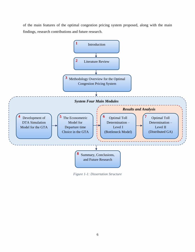
6

of the main features of the optimal congestion pricing system proposed, along with the main

findings, research contributions and future research.

Figure 1-1: Dissertation Structure

Summary, Conclusions,

and Future Research

8

Introduction 1

Literature Review 2

Methodology Overview for the Optimal

Congestion Pricing System

3

Results and Analysis

Optimal Toll

Determination –

Level II

(Distributed GA)

7 Optimal Toll

Determination –

Level I

(Bottleneck Model)

6

System Four Main Modules

Development of

DTA Simulation

Model for the GTA

4 The Econometric

Model for

Departure time

Choice in the GTA

5

7

2. Literature Review

This chapter starts with a theoretical background of the main economic models of congestion

pricing, along with their objectives and implications. A literature review of the state-of-art and

the state-of-play of congestion pricing is then provided. The chapter concludes with a summary

of the limitations in the congestion pricing models developed/implemented that motivated this

research.

2.1. Introduction to Congestion Pricing: The Economic Perspective

There are two main traffic flow modelling approaches for optimal congestion pricing; namely,

static and dynamic models. In static models, static demand and cost curves are used for

modelling, and the result are therefore static tolls (fixed over a period of time). Static pricing

assumes a static demand curve for each congested link and time period, which means that in

response to congestion level and the congestion price charged, people who are priced out either

stay at home, carpool, take transit, or move to uncongested (free-flow) times or routes.

Furthermore, this pricing model assumes that people who are priced out do not dynamically shift

to other congestible time periods (i.e. alter their departure time) nor to other congestible parts of

the network.

In dynamic models, on the other hand, the variations of traffic demand with time are captured;

accordingly, these models produce dynamic tolls that correspond to traffic dynamics. The details

of static and dynamic congestion pricing models are discussed in the following subsections.

2.1.1. Static Pricing Models

Within the conventional static models in congestion pricing, two approaches might be followed

to set road charges/prices; namely, profit maximizing pricing and social-welfare maximizing

pricing. The difference between the two is very significant. In general, as shown in Figure 2-1,

the ‘Demand’ represents the change in the quantity purchased to price; whereas the ‘Average

Cost’ (AC) is the total production cost divided by the total quantity produced; the ‘Marginal

Cost’ (MC) is defined as the change in total cost required to increase the output by one unit; and

the ‘Marginal Revenue’ (MR) denotes the change in total revenue associated with an increase in

output by one unit.

8

If the road is not priced (i.e., free-of-charge travel), demand and cost equilibrate when the AC

curve intersects with the demand curve, as shown by point x in Figure 2-1. However, the

marginal cost at this flow level is higher than the average cost, as the average cost does not

consider the external cost of congestion, or the delay a traveller imposes on all other travellers.

This ignored external cost of congestion component is viewed as social subsidy, i.e. a cost borne

by society (all travellers) for which each individual traveller does not pay. The two pricing

approaches are described as follows:

Profit Maximizing Pricing: If prices are set to maximize profits (defined as the difference

between the total revenue and the total cost), we determine equilibrium in an unregulated

environment resulting in what is known as ‘monopoly price’ (Pm), which is the price

consistent with the output where the Marginal Revenue equals the Marginal Cost as follows:

Profit = Total Revenue (TR) – Total Cost (TC)

To maximize profit with respect to volume of production (Q):

ΔTR/ΔQ = ΔTC/ΔQ

i.e., Marginal Revenue (MR) = Marginal Cost (MC)

Social-Welfare Maximizing Pricing: If prices are set to maximize the social welfare (defined

as the difference between the total benefits and the total costs), we determine a ‘marginal-

cost price’ (Pmc), which is the price consistent with the output where the Marginal Cost meets

the Demand curve.

Figure 2-1 illustrates the difference between both pricing rules (monopoly vs. marginal-cost).

In transportation, marginal-cost pricing means that each traveller faces a perceived full-cost

price (i.e., the travel cost in addition to the road charges imposed) equal to his/her activity's

social marginal cost (i.e., the monetary value of the travel time incurred by a traveller in

addition to the extra time incurred by the existing travellers due to the entrance of that new

traveller to the system).

9

Figure 2-1: Monopoly Price Pm vs. Marginal-Cost Price Pmc

Depending on the policies and constraints in place, social-welfare maximizing pricing may be

associated with two pricing schemes; namely, first-best pricing and second-best pricing.

First-best pricing: entails system-wide pricing. However, doing so in practice is often

impossible, as various constraints on what prices can be charged must be considered (for

example, the political necessity of making ‘free’ options available).

Second-best pricing: involves optimizing social welfare given some constraints on policies;

for example, the inability to price all links in a network, to distinguish between classes of

users or vehicles, or to vary tolls continuously over time.

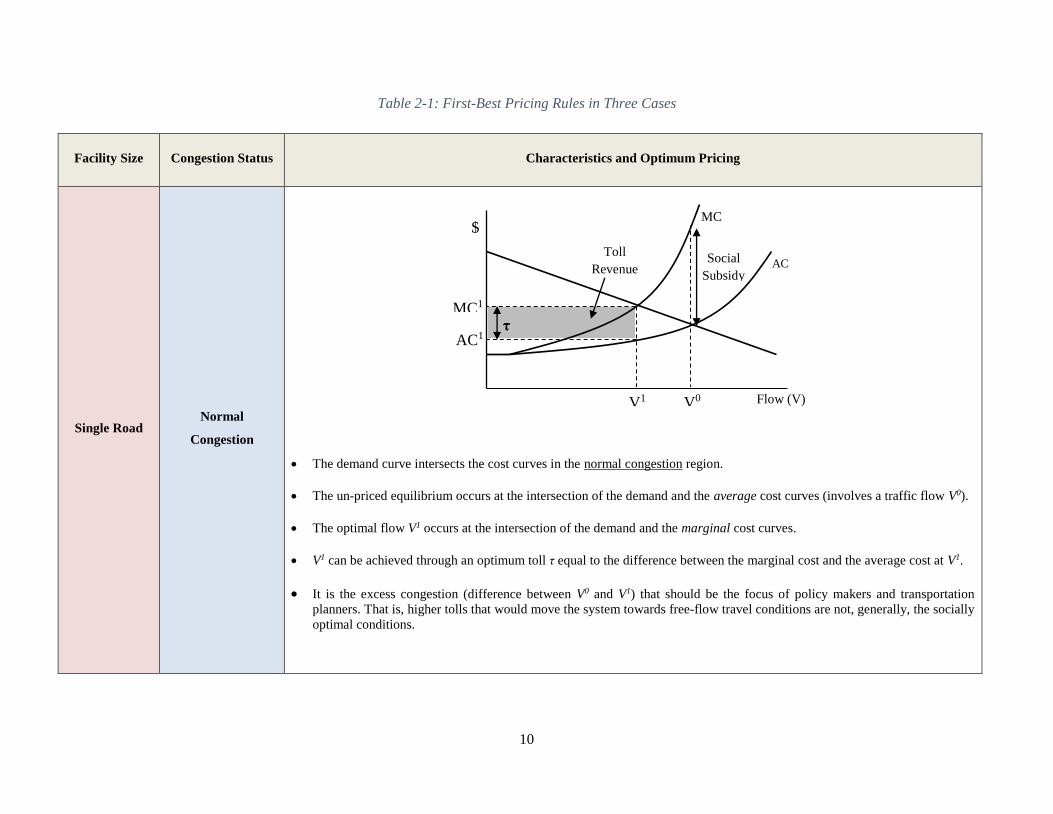
Table 2-1 summarizes the first-best pricing rules for three cases: single road at normal

congestion (where the density is below the critical density), single road at hyper-congestion

(where the density exceeds the critical density), and an entire network at normal congestion.

Finally, it should be noted that static models are appropriate only when traffic conditions do not

change quickly, or when it is thought sufficient to focus on average traffic levels over extended

periods of time, which is not the case in most large cities. In other words, static models do not

capture transportation network dynamics, such as changes in demand over time, congestion,

bottlenecks, and queue spill-backs. Dynamic models can generally overcome such limitations, as

will be illustrated in the following section.

10

Table 2-1: First-Best Pricing Rules in Three Cases

Facility Size Congestion Status Characteristics and Optimum Pricing

Single Road Normal

Congestion

The demand curve intersects the cost curves in the normal congestion region.

The un-priced equilibrium occurs at the intersection of the demand and the average cost curves (involves a traffic flow V0).

The optimal flow V1 occurs at the intersection of the demand and the marginal cost curves.

V1 can be achieved through an optimum toll τ equal to the difference between the marginal cost and the average cost at V1.

It is the excess congestion (difference between V0 and V1) that should be the focus of policy makers and transportation

planners. That is, higher tolls that would move the system towards free-flow travel conditions are not, generally, the socially

optimal conditions.

Flow (V)

$

AC Toll

Revenue

MC

Social

Subsidy

MC1

AC1 τ

V1 V0

11

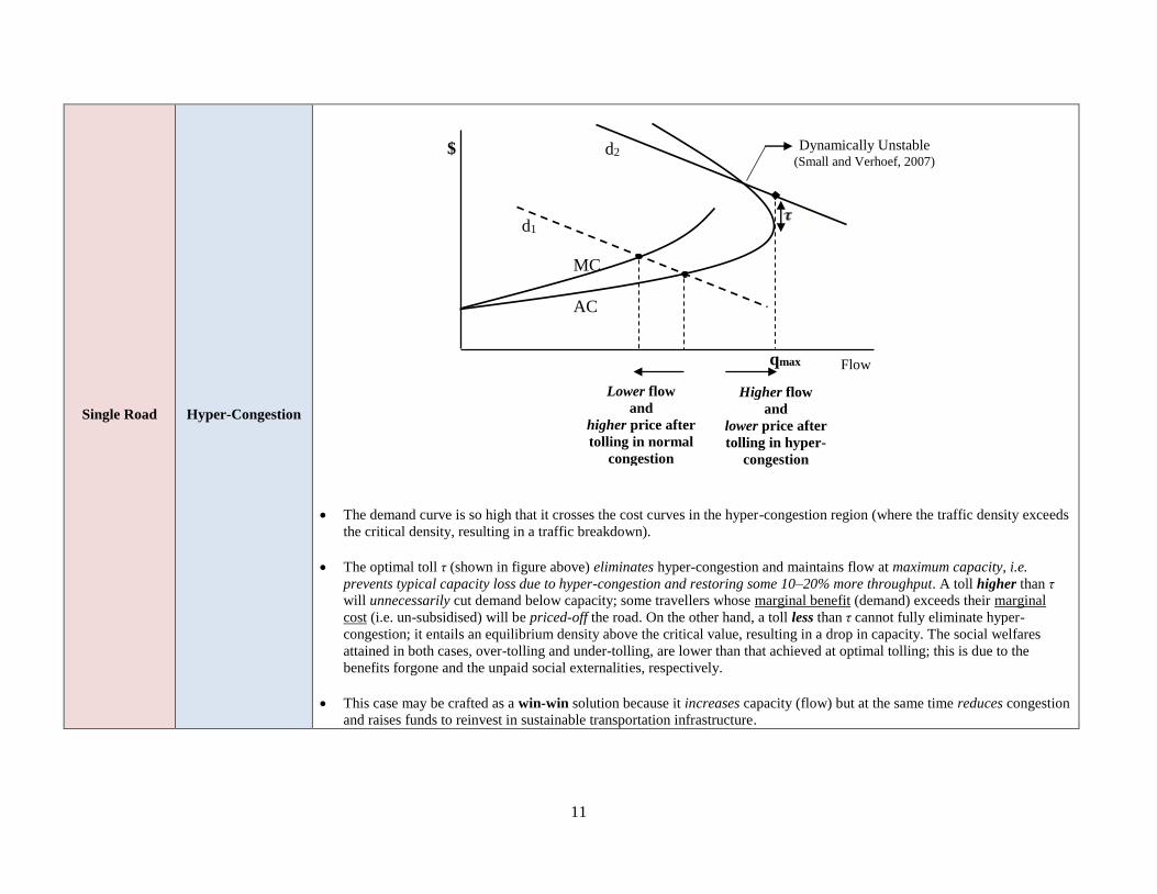
Single Road Hyper-Congestion

The demand curve is so high that it crosses the cost curves in the hyper-congestion region (where the traffic density exceeds

the critical density, resulting in a traffic breakdown).

The optimal toll τ (shown in figure above) eliminates hyper-congestion and maintains flow at maximum capacity, i.e.

prevents typical capacity loss due to hyper-congestion and restoring some 10–20% more throughput. A toll higher than τ

will unnecessarily cut demand below capacity; some travellers whose marginal benefit (demand) exceeds their marginal

cost (i.e. un-subsidised) will be priced-off the road. On the other hand, a toll less than τ cannot fully eliminate hyper-

congestion; it entails an equilibrium density above the critical value, resulting in a drop in capacity. The social welfares

attained in both cases, over-tolling and under-tolling, are lower than that achieved at optimal tolling; this is due to the

benefits forgone and the unpaid social externalities, respectively.

This case may be crafted as a win-win solution because it increases capacity (flow) but at the same time reduces congestion

and raises funds to reinvest in sustainable transportation infrastructure.

Dynamically Unstable (Small and Verhoef, 2007)

Higher flow

and

lower price after

tolling in hyper-

congestion

Lower flow

and

higher price after

tolling in normal

congestion

d2

AC

MC

d1

Flow

$

qmax

12

Network Normal

Congestion

This case highlights the correspondence between the economic perspective of pricing (maximizing social welfare) and the

traffic engineering perspective (system optimal traffic conditions).

That is, first-best tolling on a complete network is proved to satisfy system optimal conditions (where the total travel time

in the network is minimised) rather than user equilibrium conditions (where no one can improve his/her travel time by

switching routes; Small and Verhoef, 2007).

13

2.1.2. Dynamic Pricing Models

Dynamic models take into consideration that congestion peaks over time then subsides.

Therefore, in addition to hyper-congestion-free travel time, there is a delay component that peaks

with congestion as well, which travellers need to take into account.

Dynamic models, in general, assume that road users have a desired arrival time t*, deviations

from which imply early or late schedule-delay costs. Travellers who must arrive on time during

the peak encounter the most delay i.e. there is a trade-off between avoiding congestion delay and

arriving too early or too late.

The basic Bottleneck Model is the most widely used conceptual model of dynamic congestion

(Small and Verhoef, 2007). It assumes that travellers are homogeneous and have the same

desired arrival time, t*. Moreover, the model involves a single "bottleneck" with a kinked

performance function; i.e., for arrival rates of vehicles not exceeding the bottleneck capacity and

in absence of a queue, the bottleneck's outflow is equal to its inflow, and no congestion (delay)

occurs. When a queue exists, vehicles exit the queue at a constant rate equal to the bottleneck

capacity Vk.

The total number of travellers that enters the system ultimately exits the system after having

queued for a while. The optimal toll in this case attempts to “flatten” the peak, i.e. to spread the

demand evenly over the same time period. The price is set such that the inflow equals road

capacity, which in turn equals the outflow. The optimal tolled-equilibrium exhibits the same

pattern of exits from the bottleneck as the un-priced equilibrium, but it has a different pattern of

entries. Pricing affects the pattern of entries with a triangular toll schedule, with two linear

segments, which replicate the pattern of travel delay costs in the un-priced equilibrium. This

optimal toll results in the same pattern of schedule-delay cost as in the un-priced equilibrium, but

produces zero travel delay cost (i.e. no travel delays exist in the optimal case). Instead of

queueing-delay, travellers trade-off the amount of toll to be paid vs. schedule-delay such that a

traveller that arrives right on time t* pays the highest toll. The resulting tolled-equilibrium

queue-entry pattern therefore satisfies an entry rate equal to the capacity Vk. The basic

Bottleneck Model would work well only for a bridge-like case where people do not have routing

options, i.e. their reaction to tolling is limited to departure time variation.

14

In conclusion, the main benefit of static marginal-cost congestion pricing is to achieve an

optimum level of traffic flow by forcing travellers to pay the full cost of congestion externalities

to society. On the other hand, dynamic congestion models suggest that a main source of

efficiency gains from optimal pricing would be the rescheduling of departure times (temporal

distribution) from the trip origin.

Based on the theoretical approaches of congestion pricing discussed in this section in addition to

other practical schemes implemented in some major cities (e.g. London, Stockholm, and

Singapore), Table 2-2 provides a summary of different pricing policies, their objectives and

impacts and how they relate, if at all, to optimal pricing presented above (where the black filled

circles, in the table, denote a strong relation and so on). Although the classification in Table 2-2

is highly subjective and reflects the author’s view, it is meant to provide a ‘high-level’ analysis

of different policies to be followed for a certain objective sought by roadway authorities and

highway agencies.

15

Table 2-2: Congestion Pricing - Objectives and Policies

Policy

options

Main objectives/impacts

Examples of each

policy Reduce

downtown

traffic

Encourage

carpooling

Maximize

profits

Control traffic

(temporal/

spatial)

Reduce

auto-

mobile use

Maximize social

welfare (system

optimal)

Alter

departure

time choice

Cordon tolls

London Congestion

Pricing

Stockholm

Congestion Pricing

HOT lanes

I-15 HOT Lanes,

San-Diego, CA

I-394 in Minnesota

SR-167 in Seattle

Monopoly

pricing

ETR 407 (Express

Toll Route), ON,

Canada

Variable

tolls

Singapore Electronic

Road Pricing

Distance-

based fees

"MileMeter", Texas,

US

"Real Insurance

PAYD", Australia

First-best

pricing

----

Bottleneck

pricing

----

16

2.2. State-of-the-Art

According to Xu and Ben-Akiva (2009), current congestion pricing-related research is generally

classified into two main categories. The first involves studies related to developing general

frameworks of congestion pricing, as a traffic control policy. On the other hand, the second

category focuses on users' behavioural responses to congestion pricing. This section is divided

into three parts: the first two introduce some studies conducted so far in each of the above two

categories, whereas the third part presents some research related to spending congestion pricing

revenues.

2.2.1. General Congestion Pricing Framework

Studies related to developing general congestion pricing frameworks may focus on one of two

aspects: analysis models and simulation models. Analysis models, in general, concentrate on

theoretical viewpoints without being implemented on real networks, whereas simulation models

focus on the application of the algorithm and are usually less complex but more applicable.

2.2.1.1. Analysis Models

As mentioned before, this research strand considers the correctness and completeness of the

model, rather than its applications. The model is usually quite complex and requires complete

information about the network and its users. While providing some theoretical perspectives and

useful insights, the model can hardly be applied in practice. Some relevant studies are discussed

in this section.

Hall (2013) extended an existing standard dynamic congestion model to reflect the additional

traffic externality induced from the decreased throughput observed at the critical road density.

This study used survey and travel time data to estimate the joint distribution of driver preferences

over arrival time, travel time, and tolls. The author applied his model on a single highway and

showed (through calculations) that as long as some rich drivers use the highway at the peak of

rush hour, adding tolls to a portion of the lanes (up to half) helps all road users, even before

revenue is spent.

17

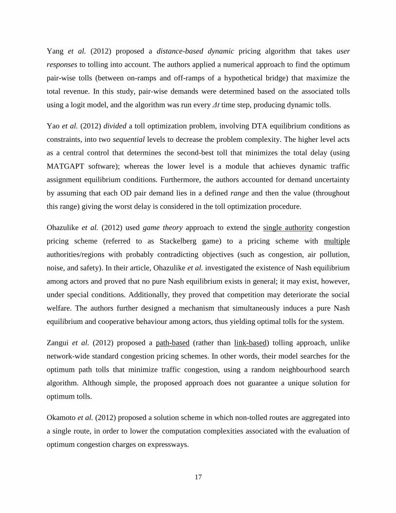
Yang et al. (2012) proposed a distance-based dynamic pricing algorithm that takes user

responses to tolling into account. The authors applied a numerical approach to find the optimum

pair-wise tolls (between on-ramps and off-ramps of a hypothetical bridge) that maximize the

total revenue. In this study, pair-wise demands were determined based on the associated tolls

using a logit model, and the algorithm was run every Δt time step, producing dynamic tolls.

Yao et al. (2012) divided a toll optimization problem, involving DTA equilibrium conditions as

constraints, into two sequential levels to decrease the problem complexity. The higher level acts

as a central control that determines the second-best toll that minimizes the total delay (using

MATGAPT software); whereas the lower level is a module that achieves dynamic traffic

assignment equilibrium conditions. Furthermore, the authors accounted for demand uncertainty

by assuming that each OD pair demand lies in a defined range and then the value (throughout

this range) giving the worst delay is considered in the toll optimization procedure.

Ohazulike et al. (2012) used game theory approach to extend the single authority congestion

pricing scheme (referred to as Stackelberg game) to a pricing scheme with multiple

authorities/regions with probably contradicting objectives (such as congestion, air pollution,

noise, and safety). In their article, Ohazulike et al. investigated the existence of Nash equilibrium

among actors and proved that no pure Nash equilibrium exists in general; it may exist, however,

under special conditions. Additionally, they proved that competition may deteriorate the social

welfare. The authors further designed a mechanism that simultaneously induces a pure Nash

equilibrium and cooperative behaviour among actors, thus yielding optimal tolls for the system.

Zangui et al. (2012) proposed a path-based (rather than link-based) tolling approach, unlike

network-wide standard congestion pricing schemes. In other words, their model searches for the

optimum path tolls that minimize traffic congestion, using a random neighbourhood search

algorithm. Although simple, the proposed approach does not guarantee a unique solution for

optimum tolls.

Okamoto et al. (2012) proposed a solution scheme in which non-tolled routes are aggregated into

a single route, in order to lower the computation complexities associated with the evaluation of

optimum congestion charges on expressways.

18

2.2.1.2. Simulation Models

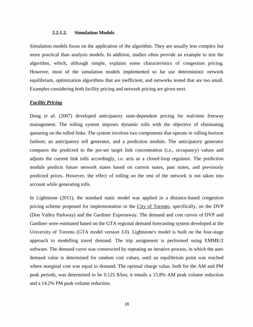
Simulation models focus on the application of the algorithm. They are usually less complex but

more practical than analysis models. In addition, studies often provide an example to test the

algorithm, which, although simple, explains some characteristics of congestion pricing.

However, most of the simulation models implemented so far use deterministic network

equilibrium, optimization algorithms that are inefficient, and networks tested that are too small.

Examples considering both facility pricing and network pricing are given next.

Facility Pricing

Dong et al. (2007) developed anticipatory state-dependent pricing for real-time freeway

management. The tolling system imposes dynamic tolls with the objective of eliminating

queueing on the tolled links. The system involves two components that operate in rolling horizon

fashion; an anticipatory toll generator, and a prediction module. The anticipatory generator

compares the predicted to the pre-set target link concentration (i.e., occupancy) values and

adjusts the current link tolls accordingly, i.e. acts as a closed-loop regulator. The prediction

module predicts future network states based on current states, past states, and previously

predicted prices. However, the effect of tolling on the rest of the network is not taken into

account while generating tolls.

In Lightstone (2011), the standard static model was applied in a distance-based congestion

pricing scheme proposed for implementation in the City of Toronto, specifically, on the DVP

(Don Valley Parkway) and the Gardiner Expressway. The demand and cost curves of DVP and

Gardiner were estimated based on the GTA regional demand forecasting system developed at the

University of Toronto (GTA model version 3.0). Lightstone's model is built on the four-stage

approach to modelling travel demand. The trip assignment is performed using EMME/2

software. The demand curve was constructed by repeating an iterative process, in which the auto

demand value is determined for random cost values, until an equilibrium point was reached

where marginal cost was equal to demand. The optimal charge value, both for the AM and PM

peak periods, was determined to be 0.125 $/km; it entails a 15.8% AM peak volume reduction

and a 14.2% PM peak volume reduction.

19

De Palma et al. (2005) explored a policy of "no-queue tolling". In this policy, time-varying tolls

are imposed selectively on a road network with the objective of eliminating queueing on the

tolled links. Moreover, the authors classified "no-queue tolling" as third-best pricing, because the

effects of the tolls on other links are disregarded. In their study, De Palma et al. used a dynamic

traffic simulator to compute no-queue tolls for individual links and cordon rings on a laboratory

network. Based on the results obtained, the authors recommend initiating third-best tolling

schemes on real networks rather than waiting a long time for comprehensive congestion pricing

(requiring extensive information on speed-flow curves and demand elasticities) to become

feasible.

In Bar-Gera and Gurion (2012), a facility pricing project was presented, implemented in Tel-

Aviv on a single left lane dedicated to public transport, high-occupancy vehicles, and toll payers.

The system includes a dynamically responsive toll-setting mechanism that guarantees a certain

level of service (speed) on the fast lane as well as a sufficient utilization (flow). The toll is

dynamically set, in a control centre, based on two components: a predictive component that

estimates the demand and willingness to pay, in addition to a feedback component that is used to

adjust the toll automatically, based on real-time measurements (Leonhardt et al., 2012).

Moreover, the project involves a free park-and-ride facility along the way that enables users to

carpool or to switch to a free shuttle service to downtown, in addition to an auxiliary right lane

connecting an on-ramp in the middle of the facility to an off-ramp at the western exit from the

facility.

Network Pricing

Verhoef (2002) developed an algorithm to find second-best tolls where not all links of a

congested transportation network can be tolled. Furthermore, a simulation model was used to

study the performance of the algorithm for various archetype pricing schemes; e.g. a toll-cordon,

pricing of a single major highway, and pay-lanes and free-lanes on major highways.

Kazem (2012) tested and compared many pricing scenarios (e.g. flat, distance-based, and peak

tolls) in a study area in the southern California region. The pricing scenarios were obtained by

consulting public groups along with transportation agencies; i.e., no theoretical rationale governs

the pricing patterns presented.

20

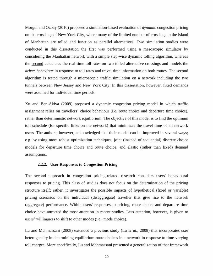
Morgul and Ozbay (2010) proposed a simulation-based evaluation of dynamic congestion pricing

on the crossings of New York City, where many of the limited number of crossings to the island

of Manhattan are tolled and function as parallel alternatives. Two simulation studies were

conducted in this dissertation the first was performed using a mesoscopic simulator by

considering the Manhattan network with a simple step-wise dynamic tolling algorithm, whereas

the second calculates the real-time toll rates on two tolled alternative crossings and models the

driver behaviour in response to toll rates and travel time information on both routes. The second

algorithm is tested through a microscopic traffic simulation on a network including the two

tunnels between New Jersey and New York City. In this dissertation, however, fixed demands

were assumed for individual time periods.

Xu and Ben-Akiva (2009) proposed a dynamic congestion pricing model in which traffic

assignment relies on travellers’ choice behaviour (i.e. route choice and departure time choice),

rather than deterministic network equilibrium. The objective of this model is to find the optimum

toll schedule (for specific links on the network) that minimizes the travel time of all network

users. The authors, however, acknowledged that their model can be improved in several ways;

e.g. by using more robust optimization techniques, joint (instead of sequential) discrete choice

models for departure time choice and route choice, and elastic (rather than fixed) demand

assumptions.

2.2.2. User Responses to Congestion Pricing

The second approach in congestion pricing-related research considers users' behavioural

responses to pricing. This class of studies does not focus on the determination of the pricing

structure itself; rather, it investigates the possible impacts of hypothetical (fixed or variable)

pricing scenarios on the individual (disaggregate) traveller that give rise to the network

(aggregate) performance. Within users' responses to pricing, route choice and departure time

choice have attracted the most attention in recent studies. Less attention, however, is given to

users’ willingness to shift to other modes (i.e., mode choice).

Lu and Mahmassani (2008) extended a previous study (Lu et al., 2008) that incorporates user

heterogeneity in determining equilibrium route choices in a network in response to time-varying

toll charges. More specifically, Lu and Mahmassani presented a generalization of that framework

21

to incorporate joint consideration of route and departure time as well as heterogeneity in a wider

range of behavioural characteristics. The model explicitly considers heterogeneous users with

different values of time and values of (early or late) schedule-delay in their joint choice of

departure times and paths characterized by a set of trip attributes that include travel time, out-of-

pocket cost, and schedule-delay cost. Furthermore, the model was applied to a relatively small

network (180 nodes, 445 links, and 13 zones) through a simulation-based algorithm. The authors

acknowledged that their model suffers from computational limitations in a large network setting.

Lu and Mahmassani (2011) extended the algorithm by incorporating the heterogeneity in users’

preferred arrival time (PAT).

In a study carried out at University Drive (Burnaby, BC) based on SP surveys conducted at a

Vancouver suburb, Washbrook et al. (2006) demonstrated a method for estimating SOV (Single-

Occupant Vehicle) commuter responses to policies introducing financial disincentives for driving

alone (road charges and parking charges) and improvements to alternative modes. More

specifically, 548 commuters from a Greater Vancouver suburb who drive alone to work

completed a discrete choice experiment (DCE) in which they chose between driving alone,

carpooling or taking a hypothetical express bus service when choices varied in terms of time and

cost attributes. Interesting results were reached in this study. For example, increases in drive

alone costs will lead to greater reductions in SOV demand than increases in SOV travel time or

improvements in the times and costs of alternatives beyond a base level of service. Accordingly,

the authors suggest that policy makers interested in reducing demand for auto travel should place

at least as much emphasis on financial disincentives for auto use as they do on improving the

supply of alternative travel modes.

In a study conducted at the University of Toronto by Sasic and Habib (2013), discrete choice

models were developed to describe mode-choice and departure time choice in the GTHA. The

empirical models were then used to evaluate mode and time switching behaviour in response to

combined variable transit pricing with peak congestion pricing policies. The results reported in

that study suggest that a policy involving a road toll would have a larger effect on shifting travel

demand over time than any other policies not including road tolls.

Liu et al. (2011) presented the current practice of modelling the impact of roadway tolls with the

mode choice model. The study revealed four dimensions of analysis that have a significant

22

influence on mode choice, including socioeconomic (e.g. household income and number of

workers), travel cost (e.g. parking, gasoline, maintenance, tolls and fares), temporal (e.g. on-

vehicle time, walk time, transfer wait time and headway), and categorical (e.g. transit strike,

seasonal variation and alternative-specific intangibles).

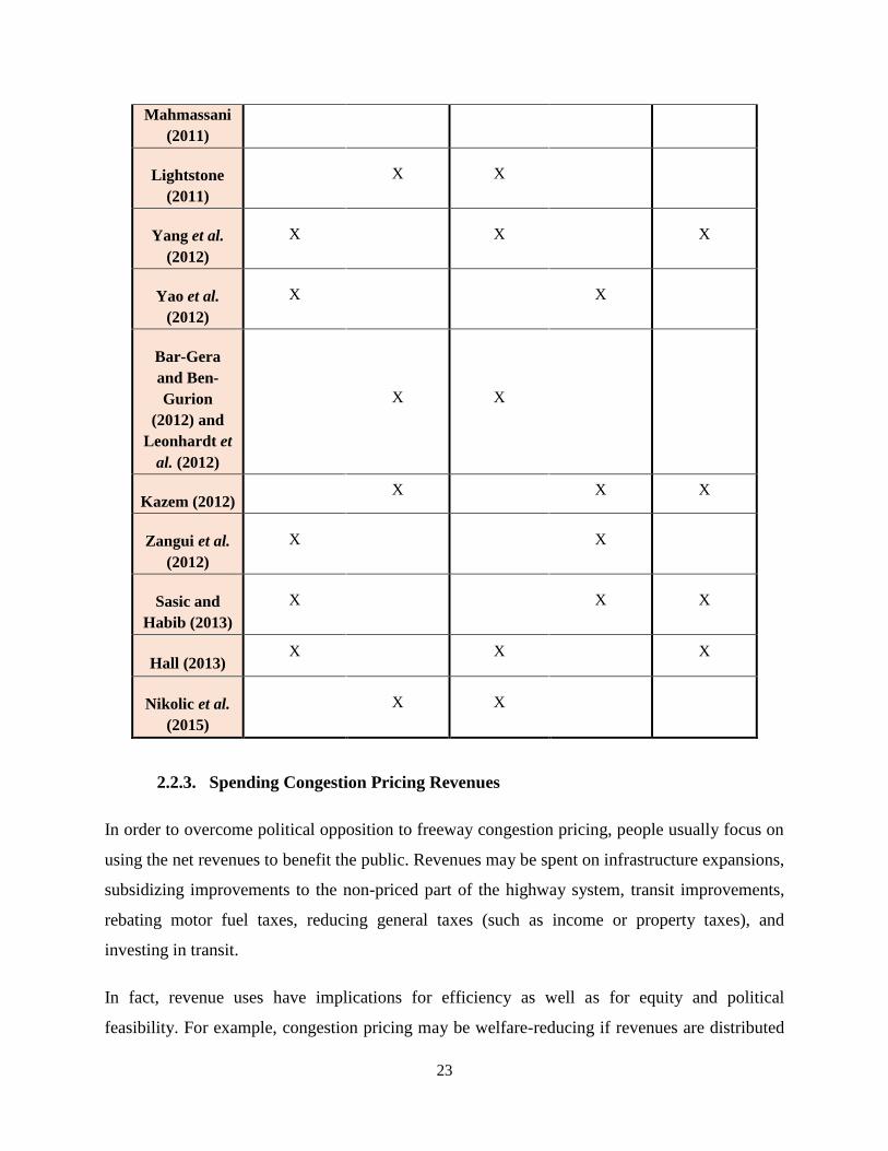
Table 2-3 provides a comparison between the different congestion pricing-related studies

reviewed so far. The studies are classified/compared based on the pricing approach adopted, the

size of the tolling scenario, and whether or not user behaviour was considered.

Table 2-3: Congestion Pricing-related Studies: Comparison

Criterion

Study

Theoretical

(Analysis)

Approach

Practical

(Simulation)

Approach

Facility-

Based

Network-

Based

User

Behaviour

Component

Verhoef

(2002) X X

De Palma et

al. (2005) X X

Washbrook

et al. (2006) X X X

Dong et al.

(2007)

X X

Xu and Ben-

Akiva (2009)

X X X

Duranton

and Turner

(2011)

X X X

Morgul and

Ozbay (2010)

X X X

Lu and X X X

23

Mahmassani

(2011)

Lightstone

(2011)

X X

Yang et al.

(2012)

X X X

Yao et al.

(2012)

X X

Bar-Gera

and Ben-

Gurion

(2012) and

Leonhardt et

al. (2012)

X X

Kazem (2012) X X X

Zangui et al.

(2012)

X X

Sasic and

Habib (2013)

X X X

Hall (2013) X X X

Nikolic et al.

(2015)

X X

2.2.3. Spending Congestion Pricing Revenues

In order to overcome political opposition to freeway congestion pricing, people usually focus on

using the net revenues to benefit the public. Revenues may be spent on infrastructure expansions,

subsidizing improvements to the non-priced part of the highway system, transit improvements,

rebating motor fuel taxes, reducing general taxes (such as income or property taxes), and

investing in transit.

In fact, revenue uses have implications for efficiency as well as for equity and political

feasibility. For example, congestion pricing may be welfare-reducing if revenues are distributed

24

in a lump-sum manner, because doing so discourages labour supply; non-wage income

discourages labour supply. On the other hand, when revenues are used to reduce/rebate the

distorting labour taxes, the usual efficiency advantage of such tax reductions is magnified.

Many congestion pricing projects in US considered integrating transit with congestion pricing

by, for example, extending HOT lanes to accommodate bus rapid transit (BRT) services and

therefore increasing transit ridership (e.g. I-15 BRT). Previous studies in Belgium, however,

have found that a marginal increase in peak-period road prices yields the highest benefit when

revenue is spent on road capacity expansion. However, it yields negative benefit when it is spent

on public transportation, unless the degree of social inequality aversion is very high. This latter

result is mainly because public transportation is already highly subsidized in this specific study

region, and it illustrates a critical point about congestion pricing: because the revenues are

typically large compared to the value of the time savings, inefficient spending of those revenues

can completely undo the net benefits of the policy (Small and Verhoef, 2007).

As for infrastructure expansion, Rouwendal and Verhoef (2006) discuss the conceptual link

between optimal congestion pricing and road capacity. These authors suggest that a useful way

of increasing public acceptability of congestion pricing would be to introduce a close

relationship between toll revenues and investment in road capacity. In their article, Rouwendal

and Verhoef build upon a theorem derived by Mohring and Harwitz (1962). This theorem states

that the revenues from the first-best optimal toll match the cost of the optimal amount of

infrastructure, under two conditions. The first condition requires that travel costs remain constant

if the number of trips and the capacity of the infrastructure change in the same proportion,

whereas the second one requires that there be no scale effects in the construction of

infrastructure. For road infrastructure, the first condition is generally acceptable and only small

deviations from condition two have been revealed in empirical research. Moreover, the theorem

remains valid if road maintenance and deviations from perfect competition on the land market

are taken into account. The theorem therefore suggests that in a long-run setting, road transport

may be self-financing if prices are set equal to marginal costs and road capacity is adjusted to its

optimal level.

25

King et al. (2007) recommend that toll revenues be given to city governments where highways

pass through. They argue that such a policy is fair because these cities bear the local external

costs of a regional system. They also argue that the policy is efficient because cities are already

an organized and effective lobby group. Their aim is not to eliminate losers from road pricing,

but rather to create gainers with sufficient motivation to overcome opposition to it.

Moreover, Poole (2011) discussed several possible uses of pricing revenues and the

consequences of each of them. The most commonly proposed use of revenues is to expand non-

driving alternatives for those tolled off the freeways, inspired by the successful London and

Stockholm implementations. Poole reported several problems with this approach, if applied in a

U.S. context. Those two European systems are cordon-price congestion pricing, aimed at

reducing traffic in traditional CBDs that already have much higher transit mode share than any

large congested U.S. metro area. Many-to-one radial transit systems are a good fit for serving the

CBDs of traditional mono-centric urban areas. Yet they are a relatively poor fit for serving the

many-to-many commuting situation of large U.S. metro areas whose primary commuting pattern

for several decades has been suburb-to-suburb. Another proposal, presented in that article, is that

100% of the net revenues be allocated to the jurisdictions through which priced freeways extend,

in proportion to route-miles or lane-miles. There would be no restrictions on the use of these

funds; they would become a new source of general revenue for those cities. Nevertheless, the

author mentioned that this proposal might be an example of “monopoly exploitation” version of

congestion pricing, since it does not direct resources (i.e., pricing revenues) to locations and

projects where prices indicate that increased investment is needed. In other words, the proposal

disregards the users-pay/users-benefit principle.

In conclusion, there is no unique strategy that can be referred to as the most efficient way of

spending pricing revenues. Instead, case-specific studies should be conducted for each region

(considering implementing congestion pricing projects) to determine the most appropriate use of

revenues in that region.

2.3. State-of-Play Worldwide

The United States, the United Kingdom, France, Norway, Sweden, Germany, Switzerland,

Singapore, and Australia have implemented major congestion pricing projects. The projects may

26

be classified as being facility-based or area-based. In this section, the main characteristics of

some implemented pricing schemes (in both classes) will be discussed to illustrate the variety of

ways in which congestion pricing has been implemented worldwide.

2.3.1. Facility-Based Projects

This category refers to congestion pricing applications that allow users to choose between two

adjacent roadways (or lanes within the same road): one tolled but free-flowing and another free

but congested. Highway 407 (aka ETR 407), in Canada, is a good example of such projects.

Additionally, several congestion pricing applications have been deployed in the United States;

for example, I-15 in San Diego, I-394 in Minnesota and SR-167 in Seattle. These programs apply

dynamic pricing strategies, using real-time information collected from loop detectors (Dong et

al., 2007).

ETR 407 (Express Toll Route)

This is a multi-lane electronic highway running 107 km across the top of the GTA from Highway

403 (in Oakville) to Highway 48 (in Markham). ETR 407 was constructed in a partnership

between "Canadian Highways International Corporation" and the Province of Ontario and

currently owned by "407-ETR International Inc.". The fees are distance-based and variable

according to zone congestion-level (light and regular), day of the week (weekday, weekend and

holidays), and time of day (peak period, peak hours and off-peak). Speeds on Highway 407 are

almost double those on other free highways during peak periods.

It should also be noted that, unlike US congestion pricing applications, tolls on ETR 407 are not

regulated; i.e. they differ according to a fixed schedule that is posted (and updated if necessary)

on their website. To what extent this pattern reflects traffic threshold regulations (provincial

safety and environmental standards and to relieve congestion on alternative public highways) and

to what extent profit maximization is achieved, is difficult to tell (Lindsey, 2007).

I-15 HOT Lanes, San-Diego, CA

This project was implemented in 1996 along the 13 km HOV section of I-15 in San Diego. The

HOT lanes on I-15 are now about 32 km long. The program determines toll values by comparing

aggregated volumes obtained from two observation intervals against volume thresholds

27

prescribed in a look-up table. The tolls are updated every 6 min ($0.5–4) and then displayed on

variable message signs. An evaluation study of this dynamic and state-dependent pricing

application for the US Department of Transportation concluded that it was successful (Dong et

al., 2007).

2.3.2. Area-Based Projects

In this type of project, users pay a fee to enter a restricted area, usually within a city centre, as

part of a demand management strategy to relieve traffic congestion within that area.

Implementations in three big cities will be presented: London, Stockholm and Singapore.

London Congestion Pricing

This was the first congestion pricing program in a major European city (in service since 2003). It

involves an £11.50 daily cordon fee (flat price) for driving in the "Central London Congestion

Pricing Zone" during weekdays (i.e. from 7 am to 6 pm). The fee is paid once per chargeable day

regardless of how many times the user crosses the charging zone. After one year of cordon tolls

and during charging, the traffic circulating within the zone decreased by 15%, traffic entering the

zone decreased by 18% and congestion (measured as the actual minus the free-flow travel time

per km) decreased by 30% within the zone (Santos, 2008).

Stockholm Congestion Charges

Stockholm ran a seven-month congestion charging trial (between January and July 2006), after

which public support increased. The congestion tax was then implemented on a permanent basis

on August 1, 2007. In this project, vehicles entering the inner-city area on weekdays (from 6:30

am to 6:30 pm) pay a toll that varies between $1.29–4.11 according to the time of day. Unlike

the London pricing scheme, drivers in Stockholm pay every time they cross the charging area

with a maximum daily charge of $8 per day. After implementation, traffic volumes reduced by

25%, public transit ridership increased by 40,000 users per day, and retail sales in central

Stockholm shops increased.

Singapore Electronic Road Pricing

The ERP (Electronic Road Pricing) project was implemented in Singapore in 1998, after 23

years of operating a cordon scheme with paper licenses. It covers wide regions of the island;

28

namely, the Central Business District (from 7:30 am to 7:00 pm) and expressways/outer ring

roads (from 7:30 am to 9:30 pm). Charges vary by location and time of day in 30 min steps

(adjusted quarterly depending on average speeds measured in the previous quarter). Five min toll

intervals were introduced between some 30 min steps in order to discourage motorists from

speeding up or slowing down when the toll is about to increase or decrease. Similar to

Stockholm pricing, vehicles in Singapore pay every time they cross the charging area.

2.4. Concluding Remarks

As presented throughout this chapter, there are numerous dimensions to the congestion pricing

problem that need to be considered, or at least reasonably assumed, when planning a congestion

pricing strategy. Despite the numerous studies that have contributed considerably to the state-of-

the-art and the state-of-practice in congestion pricing, they still suffer from a number of

limitations that limit their use in large and complex urban areas. Figure 2-2 summarizes the

major challenges and gaps in the existing literature that have motivated the current research.

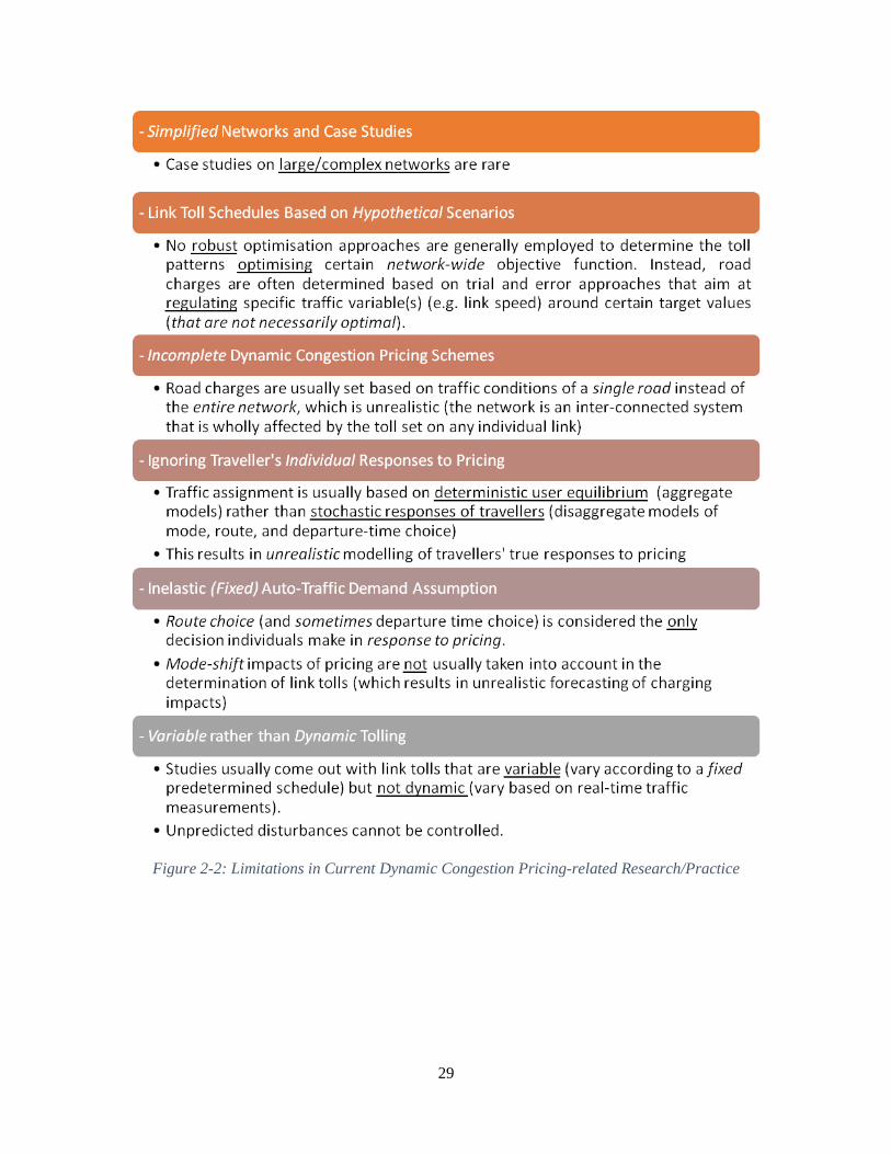
29

Figure 2-2: Limitations in Current Dynamic Congestion Pricing-related Research/Practice

30

3. Methodology Overview: Optimal Congestion Pricing System

In light of the gaps in the state-of-the art of congestion pricing, discussed in Chapter 2, this study

seeks to develop a robust system for the methodological derivation, evaluation, and optimization

of variable congestion pricing policies to manage peak period travel demand, while explicitly

capturing departure time and route choices in a large-scale dynamic traffic assignment (DTA)

simulation environment.

The study, through the extensive travel survey data available in the Greater Toronto Area (GTA),

considers the drivers’ heterogeneity in their values of (early or late) schedule-delay and desired

arrival time. Moreover, drivers’ personal and socio-economic attributes – affecting the choice of

departure times – are taken into account besides the trip-related travel time, out-of-pocket cost,

and schedule-delay cost.

The optimal variable congestion pricing policies are obtained through a bi-level procedure. The

first level involves the determination of time-dependent queue-eliminating toll structures for

congested facilities. The toll structure determination is motivated by the Bottleneck Model,

which is the most widely used conceptual model of dynamic congestion pricing (Small and

Verhoef, 2007). On the other hand, the second level involves iterative optimization (i.e., fine-

tuning) of the toll structures determined in the first level to achieve the best possible network

performance. This is achieved through further optimization of the toll structures obtained in the

first level to consider the potential route and departure time choice dynamics in response to

tolling in addition to the large-scale network interconnectivity. The second level uses a robust

iterative optimization algorithm that is run concurrently (i.e., distributed) on a parallel computing

cluster.

This chapter presents a system for the determination and evaluation – through a large-scale

simulation environment – of optimal variable congestion pricing policies as a method of spatial

and temporal traffic congestion management. The system is based on four key pillars: 1) a large-

scale calibrated dynamic traffic assignment simulation platform that is used to assess the impact

of various pricing options on routing and congestion patterns; 2) an econometric (behavioural)

model of departure time choice that is built and calibrated using regional household travel survey

data that capture the heterogeneity of travellers’ personal and socioeconomic attributes; 3) the

31

Bottleneck Model for dynamic congestion pricing, which is the theoretical basis of the initial

variable toll structure determination approach adapted here; and 4) a robust iterative distributed

optimization approach for toll structures fine-tuning to achieve the best possible network

performance. These pillars are integrated and implemented into a single system that incorporates

iterative optimization of variable tolling while looping between the departure time choice layer

and the DTA layer until departure time choices and route choices reach equilibrium, under each

tolling scenario being assessed during optimization. For the system large-scale nature and the

consequent (time and memory) computational challenges, the optimization algorithm is run

concurrently on a parallel computing cluster. The key pillars of the approach are described next.

3.1. Mesoscopic Large-Scale Dynamic Traffic Assignment (DTA) Simulation

Model

Congestion pricing is typically sought in large congested urban areas, where congestion spreads

over wide space for long peak hours. Therefore, to control traffic dynamically in large-scale

congested networks, three systems are needed concurrently: (1) a prescriptive decision-

setting/control tool (e.g. a demand or supply control policy such as congestion pricing or ramp

metering etc.), (2) a descriptive calibrated econometric departure time choice model, and (3) a

descriptive calibrated dynamic traffic assignment (DTA) model that captures route choice

dynamics and the evolution of traffic congestion resulting from travellers seeking the least-

generalized-cost routes to their destinations. A large-scale DTA simulation model is, hence,

required for optimal congestion pricing policy derivation and evaluation; a model that can

realistically capture the route choice dynamics network-wide (over time and space) resulting

from fixed or variable tolls along key corridors. It is noteworthy that these tolls would in turn

affect travellers’ departure time choice; and therefore the need to integrate both the route and

departure time choice models within the same system.

To that end, and to capture the system-wide effects of tolling in large urban areas, a mesoscopic

large-scale DTA model is used here. In a large-scale interconnected network (like the GTA)

where long-distance trips have diverse routing options, tolling relatively short highway segments

might create temporal and spatial traffic changes network-wide that go beyond the tolling

interval and the tolled segment. This necessitates conducting the simulations on a regional scale

for comprehensive policy determination and assessment.

32

In general, mesoscopic models simulate the movement of vehicles in the transportation network

in groups according to the fundamental diagrams of traffic theory. These models offer a

compromise between microscopic and macroscopic models; unlike macroscopic models, they

model individual vehicles, and unlike microscopic models, they are less computationally

demanding and hence are more suited for modelling large networks (Abdelgawad and Abdulhai,

2009).

Transportation networks are dynamic; changes in demand over time, congestion, bottlenecks,

unpredicted incidents etc. cause link travel times to change with time and cause congestion to

spillback upstream with time. Accordingly, the shortest path between certain origin-destination

pair may change over time as well. Therefore, it is important to use DTA simulation models for

the determination and assessment of spatial and temporal traffic demand management policies

like congestion pricing. These models use dynamic (i.e. time-dependent) shortest path algorithms

to find the shortest path between each origin-destination pair in the network at all possible

departure times (from the origin node).

Details related to the demand patterns, which are inputs to the mesoscopic simulation model, the

key traffic assignment control parameters, the simulated network geometry, and the simulation

model base-case calibration/validation results will be discussed in Chapter 4.

3.2. The Econometric Model for Departure Time Choice

In order to capture users' individual departure time choice responses to variable tolling, this study

uses an econometric (behavioural) departure time choice model. The model considers drivers’

socio-economic attributes and the network level-of-service attributes. This study extends a

departure time choice model recently developed at the University of Toronto (Sasic and Habib,

2013) that describes departure time choice in the Greater Toronto and Hamilton Area (GTHA).

The developed departure time choice model is a Heteroskedastic Generalized Extreme Value

(Het-GEV) model that further enhances the Choice Set Generation Logit (GenL) captivity

component developed by Swait (2001).

The Het-GEV model explicitly captures the correlation between adjacent choice alternatives (by

allowing choice alternatives to appear in multiple clusters) while the GenL form captures the

captivity of decision makers to specific choice alternatives due to schedule constraints. The GEV

33

class of models for discrete choice applications makes use of random utility maximization

theory, where each agent (traveller) is assumed to choose an alternative that maximizes its

random utility. The random utility for any alternative is defined as a systematic and a random

component (where the joint density of all random components is distributed according to the

extreme value distribution).

Two types of scale parameters are introduced in this model. These are the root scale parameter

and the nest scale parameter of a particular choice set. Moreover, the modelling framework uses

a scale parameterization approach to capture heteroskedasticity in departure time choices. This

approach also captures heterogeneity in users’ departure time choice responses to variations in

trip-related attributes (e.g. travel time and cost) at each choice interval.

The model was developed and calibrated in the original study using the Transportation

Tomorrow travel Survey (TTS) of 2006. In this study, the model was retrofitted using the latest

TTS survey of 2011 (DMG, 2015). Additionally, the schedule delay and toll cost components

were incorporated in the model variables, and their associated parameters were recalibrated

accordingly.

Details of the model choice set structure, the utility function variables, the extensions and

assumptions made to incorporate schedule-delay and toll cost components in the model variables

and the associated parameters adjustment/recalibration process, the steps followed to prepare the

data required by the model, and the retrofitted model base-case validation results are all

presented in Chapter 5.

3.3. Optimal Toll Structures Bi-Level Determination Approach

Congestion in large cities like Toronto has reached a level where demand is usually over

capacity in peak periods, resulting in long lasting queues on key corridors. Additionally, the

traffic instability occurring when traffic density exceeds the critical density (i.e. the density

corresponding to capacity) causes a significant 10–20% drop (breakdown) in capacity (Small and

Verhoef, 2007). We therefore search for an economic pricing strategy that enforces traffic pacing

(i.e., departure time rescheduling) and works towards eliminating traffic queues. Traffic pacing

ensures that demand enters the network at a rate that does not exceed capacity; hence, at least

34

theoretically, no queues or delays form. Furthermore, targeting the elimination of traffic queues

through congestion pricing will also sustain the original capacity.

In light of these benefits, we are looking for 1) time-dependent toll structures for traffic pacing

and to eliminate queues in the peak period on congested facilities while taking into consideration

the drivers’ desired work-trip arrival times and associated schedule (early or late arrival) delays

and 2) suitable toll levels to enforce proper route choices that minimize the total travel times. In

other words, we are seeking congestion pricing policies that achieve the best – spatial and

temporal – traffic distribution and infrastructure utilization to optimize the network performance

(i.e., minimize the total travel times).

For practicality and spatial equity, the tolling scheme adopted here is distance-based; toll values

are entered to the network in ($/km). Therefore, each vehicle pays according to the distance

travelled on tolled facilities. A bi-level procedure is used, as mentioned earlier, to determine the

optimal toll structures achieving the above benefits. The first level involves the determination of

time-dependent queue-eliminating toll structures for congested facilities. This is motivated by the

Bottleneck Model for optimal dynamic congestion pricing, based on the simulated base-case (no-

pricing) traffic conditions on the congested facilities to be tolled. Using the Bottleneck Model

alone to determine tolls is insufficient in large networks with numerous routing options, i.e.

when travel choices are more than just departure time choice. The second level, therefore,

involves genetic optimization to fine-tune the toll values obtained in the first level further, to

achieve the best network performance, while considering the large-scale network (route and

departure time choice) dynamics in response to tolling. This is performed through a robust

iterative optimization algorithm that is integrated to the departure time choice and DTA

simulation models, and is run concurrently (i.e., distributed) on a parallel computing cluster. The

two optimal toll determination levels are described next.

3.3.1. Level I: Initial Toll Structures Determination Based on the Bottleneck Model

for Dynamic Congestion Pricing

Dynamic models consider that congestion peaks over time then subsides. Therefore, there is a

congestion delay component that peaks with the congestion that the travellers experience.

Dynamic models assume that travellers have a desired arrival time t*; deviations from which

35

imply early or late schedule delays. Travellers who must arrive on time during the peak periods

encounter the longest delay; i.e., there is a trade-off between avoiding congestion delay and

arriving too early or too late.

The basic Bottleneck Model is the most widely used conceptual model of dynamic congestion

pricing (Small and Verhoef, 2007). It involves a single "bottleneck" and assumes that travellers

are homogeneous and have the same desired arrival time. Moreover, the model assumes that for

arrival rates of vehicles not exceeding the bottleneck capacity and in the absence of a queue, the

bottleneck's outflow is equal to its inflow; as a result, no congestion (delay) occurs. The peak

period is considered to start when the inflow exceeds the bottleneck capacity, resulting in traffic

queues and increased travel times that build up to a maximum when the inflow starts decreasing

below capacity. The peak does not end at this point of time; rather, it ends when all travellers

who entered the system (from the beginning of the peak period) ultimately exit after having

queued for a while. When a queue exists, vehicles exit the queue at a constant rate, which is the

same as the bottleneck capacity. Note that the total number of travellers that enters the system

ultimately exits the system after having queued for a while.

The optimal toll in the Bottleneck Model attempts to “flatten” the peak in order to spread the

demand (inflow) evenly over the same time period. In this case, the price is set such that the

inflow equals the bottleneck capacity, which in turn equals the outflow. The schedule-delay cost

function is assumed to be piecewise linear in the Bottleneck Model. Accordingly, pricing affects

the pattern of entries with a triangular toll schedule (that rises from zero to a maximum then falls

back to zero) replicating the pattern of travel delay costs in the un-priced equilibrium. This

results in the same pattern of schedule-delay cost as in the un-priced equilibrium, but it produces

zero travel delay cost (i.e. no travel delays exist in the optimal case). Instead of queueing delay,

travellers trade off the amount of toll to be paid versus schedule delay such that a traveller who

arrives right on time t* pays the highest toll. The resulting tolled-equilibrium queue-entry pattern

therefore satisfies an entry rate equal to the bottleneck capacity, i.e. the queue entry rate equals

the queue exit rate. Further details of the theoretical Bottleneck Model for dynamic congestion

pricing are provided in Chapter 6.

The toll structure introduced here is motivated by this theoretical bottleneck pricing theory;

where key benefits arise from rescheduling (temporal distribution) of departure times from the

36

trip origin, resulting in no (or at least less) queueing delays on tolled facilities. Initial toll

structures are determined for congested facilities based on their queueing delay patterns under

simulated base-case traffic conditions (i.e., without tolling), as will be described in detail in

Chapter 6.

3.3.2. Level II: Toll Structures Fine-Tuning Using Distributed Optimization

Algorithm

Although the Bottleneck Model provides the core concept, it is limited to the case of a single

bottleneck, where the departure time choice is the only choice travellers have to respond to

pricing. In large urban networks, there are a myriad of origin-destination pairs, trip lengths,

travellers’ schedules, desired work/school arrival times, routing options and travel behaviour that

vary across the population. These factors might affect the (departure time rescheduling) benefits

obtained from the initial toll structures determined for congested facilities in the large-scale

network. This is due to the possible temporal and spatial traffic changes network-wide (in

response to time-dependent tolling) that go beyond the tolling interval(s) and the tolled route(s),

and might bring counterproductive impacts of tolling, as will be demonstrated later.

Therefore, the proposed pricing system extends the conceptual (optimal) triangular pricing

structure suggested by the Bottleneck Model to the more complex and general case of a large

urban network. More specifically, an optimization module is integrated into the congestion

pricing system to fine-tune the initial toll structures calculated (in Level I), while considering the

network-wide dynamics that were absent in the Bottleneck Model. The fine-tuning process

involves finding (through an optimization algorithm) the optimal adjustment factors to be applied

to the initial toll structures, in order to obtain the optimal (Level II) toll values leading to the best

possible network performance.

The optimization module, integrated into the pricing system, uses a Genetic Algorithm (GA) for

optimization. The GA belongs to the class of Evolutionary Algorithms (EAs). It generates –

through an iterative process – solutions to the optimization problem using techniques inspired by

natural evolution, such as selection, mutation, and crossover. In each generation, the value of the

objective function (i.e. fitness) of every individual in the population is evaluated. The fittest

individuals are stochastically selected from the current population and possibly modified

37

(recombined and mutated) to form a new generation of candidate solutions that is then used in

the next iteration of the algorithm. The GA terminates when either a user-specified (maximum)

number of generations has been produced, or when a satisfactory level of convergence (e.g., a

solution that satisfies minimum criteria) has been reached (Back, 1996).

As mentioned, the proposed pricing system uses econometric departure time choice modelling

(based on regional travel surveys) in conjunction with DTA assignment to capture network-wide

departure time and route choice dynamics in response to each tolling scenario (solution) being

evaluated during optimization.

For the system large-scale nature and the consequent (time and memory) computational

challenges, the optimization algorithm is run concurrently on a parallel computing cluster under

a ‘Map-Reduce’ programming paradigm, as will be described later. For that purpose, a java-

based middleware for distributed in-memory processing, denoted as Apache Ignite©, is utilized

for system deployment on the parallel cluster. Moreover, the use of a large network of remote

servers – hosted on the Internet – is possible through this middleware, which allows on-demand

access to Internet-based shared resources in accordance with the application requirements.

Details of the optimization problem specifications (e.g., the optimization variables and the

objective function), the GA package used, and the middleware configuration and implementation

are presented in Chapter 7. The results and analysis of the full system implementation on a case

study in the GTA are also presented in that chapter.

3.4. The Integrated Optimal Congestion Pricing System

Figure 3-1 shows the general framework of the integrated optimal congestion pricing system

developed here. The ultimate goal of this system is to provide a tool for optimal (time-

dependent) congestion pricing policy derivation and evaluation, while taking into account the

route choice and departure time choice dimensions in large-scale regional networks. The figure

presents the system’s four key modules (described briefly in the preceding sections), the input

data provided to the system, and the data exchanged between the system modules. Further details

corresponding to the input data required by the system are provided next. Additionally, the

implementation sequence and the three levels of convergence sought (highlighted in Figure 3-1)

38

are described and illustrated through a flowchart of the optimal congestion pricing system, in

Section 3.4.2.

39

Figure 3-1: Optimal Congestion Pricing System Framework

1st

2nd

3rd

Levels of

(Iterative)

Convergence

Optimal Toll

Determination

– Level I

(Bottleneck

Model)

Optimal Toll

Determination

– Level II

(Distributed

Optimization

Algorithm)

DTA Traffic

Network

Simulator

(Route Choice)

Econometric

Model for

Departure time

Choice

Initial Toll Structures

for Congested

Facilities

t*

Time

$

Triangular toll

of the bottleneck

model

Nonlinear version

(step tolls) of the

triangular toll

structure

Tolling Intervals

Toll Structure (Time-Dependent Toll Values)

for each Congested Facility

Congested

Facilities of

Interest

(to be tolled)

Initial

(Historical)

OD Demand

Matrices

Commuters

Personal and

Socio-Economic

Attributes

Adjustment Factors

(Fine-Tuning) for

Initial Toll Structures

Network Performance

under Toll Structures

Tested

LOS

Attributes

(OD times

and costs)

Testbed (Traffic Simulation Results

under Equilibrium Route and

Departure time Choices in

Response to Tolling)

Updated

Temporal

Demand

Profiles

Optimal Toll Determination

40

3.4.1. System Input Data

Two types of data should be provided to the congestion pricing system implemented here. The

first is entered once to the testbed, highlighted in Figure 3-1, which is used to evaluate any

congestion pricing scenario. The second is related to the tolling scenario under analysis. The two

types are further described next.

3.4.1.1. Testbed-related Data

As mentioned, the congestion pricing policies to be determined and optimized by the system are

evaluated through a testbed of hybrid dynamic traffic assignment and departure time choice

behavioural models. The testbed provides detailed traffic simulation results (e.g. travel times and

costs) under equilibrium route and departure time choices, in response to tolling. It takes as

input:

1. The network topology: traffic analysis zones (TAZs), highways, major arterials, on-and-off

ramps, speed limits, traffic signal information at the major signalized intersections, etc.

2. The historical demand in the form of time-dependent origin-destination (OD) matrices for the

period of study.

3. The commuters’ personal and socio-economic attributes required by the behavioural model

for departure time choice.

The travel demand-related data used here are extracted from the latest 2011 Transportation

Tomorrow Survey (TTS; DMG, 2015). TTS is a household-based travel demand survey that is

conducted in the Greater Toronto and Hamilton Area (GTHA) every five years. The survey

provides detailed information on trips made on a typical weekday by all individuals in the

selected households. Information collected in the survey includes household-related attributes

(e.g., the number of people and the number of vehicles available for personal use), person-related

attributes (e.g., their age, driver licence availability, and work/school location), and trip-related

attributes (e.g., origin, destination, purpose, start time, and type of transportation used). Five

percent of the GTHA households are contacted by telephone and all trips made by residents 11

years of age or older on a specific weekday are recorded. Expansion factors are used to expand

the collected data to represent the total population of the survey area in the year of the survey.

The expansion factors are determined based on geographical areas and verified based on the

41

Canada Census data that are used as the control total for calculating the expansion factors (DMG,

2015).

3.4.1.2. Tolling Scenario-related Data

The congestion pricing system implemented here is designed to determine and test different

tolling scenarios, e.g. HOT lanes, congested highway sections, and cordon tolls. Toll values can

be discretized with time (up to a toll value per minute) and space (up to a toll value per link). The

following tolling scenario-related specifications should be provided to the system:

1. The facilities of interest intended to be tolled (e.g. link, corridor, or cordon): Depending on

their base-case congestion levels, the “Optimal Toll Determination – Level I” module

(described briefly in Section 3.3.1 and shown in Figure 3-1) determines whether or not each

facility of interest needs to be tolled. For those who should be tolled, the module determines

an initial toll structure for each of them, as will be described in detail in Chapter 6.

2. Spatial tolling specifications: The tolled facilities can take the form of HOT lane(s) on

congested highways, entire roads (i.e. not just one lane), or cordon tolls. A combination of

these policies can be implemented and tested in any one scenario.

3. Temporal tolling specifications: The toll interval width (during which toll is fixed over time)

and the bounds of the tolling period (i.e., start and end times of tolling) should be specified

for each facility of interest. The actual peak (hence tolling) start and end times within the

tolling period bounds are then determined by the “Optimal Toll Determination – Level I”

module.

4. The maximum allowable toll value for each facility of interest (for political reasons, say):

This value will not be exceeded in the optimal toll determination, even if doing so improves

the network performance.

3.4.2. System Flowchart

The flowchart presented in Figure 3-2 illustrates the high-level input, output, and implementation

sequence of the optimal congestion pricing system implemented in this study. As illustrated in

the figure, the system works in the following order:

- Calculate Initial Toll Structure for Each Facility of Interest in the Network: The structure

takes a nonlinear version of the price of the Bottleneck Model (i.e., step tolls rather than a

42

continuous triangular toll structure), as shown in Figure 3-1. The price is calculated based on the

base-case simulated travel times on the facility of interest; it rises from zero to a maximum then

falls back to zero when congestion decreases.

- Fine-Tune the Initial Toll Structures for Optimal Network Performance: The optimization

algorithm seeks the optimal adjustment factors to be applied to the initial tolls to achieve the best

network performance. Each factor is multiplied by the corresponding initial toll structure to

increase or decrease it. Each vector of adjustment factors – composed by the optimization

algorithm – is evaluated through a testbed of DTA and departure time choice models, as will be

described next. After evaluation, the objective function value is returned to the optimization

algorithm. The fine-tuning process is repeated iteratively until certain convergence criterion is

met. The convergence sought at this step is the 3rd level (toll structure convergence) highlighted

in Figure 3-1 and Figure 3-2.

- Apply Departure time Choice Model: The departure time choice model takes as input the toll

structures, the heterogeneous personal and socio-economic commuters’ attributes, and the

average OD travel times and costs calculated across the network from the most recent DTA

simulation run. The output of the discrete-choice model, in turn, represents the new temporal

demand patterns (with modified trip start times) due to tolling.

- Run DTA Simulation Model: The DTA simulation model takes the network topology, the toll

structures, and the anticipated demand. It performs iterative dynamic user-equilibrium (DUE)

traffic assignment, which is the 1st level of convergence (route choice convergence) highlighted

in Figure 3-1 and Figure 3-2. It results in OD travel times, updated network conditions, and

routing options given the inputs received.

- Integrate Departure time and Route Choices: The equilibrium in drivers’ behavioural responses

to pricing policies is sought by iteratively and sequentially simulating the changes in route choice

and departure time choice in response to tolling through the DTA simulator and the discrete-

choice module, respectively. More specifically, the discrete-choice module estimates the impact

of the input toll schedules given the most recent network conditions (travel times and costs) on

travellers' individual departure time choices. The updated choices are then fed back into the

dynamic traffic assignment simulator, which, in turn, produces the new network conditions and

so on, until a certain convergence criterion is met. The convergence sought is the 2nd level

(departure time choice convergence) highlighted in Figure 3-1 and Figure 3-2, after which the

43

objective function (e.g. total travel time) is calculated and returned back to the optimization

algorithm.

- Conduct Detailed Performance Analysis under Optimal Tolls: When the optimization

algorithm converges to the optimal adjustment factors (hence toll structures), a detailed analysis

is conducted to assess the impact of the optimal congestion pricing policy determined. The

analysis is carried out on three levels: (1) impact on the whole network, (2) impact on tolled

facilities and their direct parallel routes, and (3) impact on toll payers.

In the process above, three levels of equilibrium are sought. The first (inner iterative loop) is the

dynamic user equilibrium within the traffic assignment simulation model, i.e., route choice

convergence. The convergence criteria used for traffic assignment are referred to as the Relative

Gap (RG); this is a measure of how close the current assignment solution is to the User

Equilibrium (UE) network assignment (Chiu et al., 2008). The traffic assignment iterations

terminate when the RG drops below certain pre-specified convergence threshold or when a pre-

specified maximum number of iterations is reached. The second level (intermediate iterative

loop) is the equilibrium in the departure time choice model output in response to changes in the

traffic network travel times and costs under specific input toll structures; i.e., departure time

choice convergence. The intermediate loop terminates when travellers cease to change their

departure time interval, i.e. when the maximum (absolute) relative difference in the total number

of vehicles at any departure time interval drops below a pre-specified convergence threshold.

The third level (outer iterative loop) is the equilibrium in the network performance measurement

used in the optimization function, under different toll structures tested by the optimization

algorithm; i.e., toll structure convergence. The algorithm terminates when the adjustment factors

(i.e., toll structures) achieving acceptable network performance are obtained, or when a pre-set

maximum number of iterations is reached.

44

Figure 3-2: Optimal Congestion Pricing System Flowchart

No

Yes

Yes

No

Inputs

- Historical OD demand.

- Commuters’ personal

attributes.

- Base-case simulated network

attributes (times, costs, etc.).

- Tolling scenario information.

Optimal Toll Determination - Level I (Bottleneck Model - One-shot)

Determine tolling start and end times, and

initial toll structures for congested facilities.

Optimal Toll Determination - Level II (Optimization Algorithm - Iterative)

Search for the optimal adjustment factors

(fine-tuning) for initial tolls.

Convergence?

Apply the DCM to calculate each

commuter’s new departure time choice.

Update the input demand

profile of the DTA simulator.

Convergence?

Run the DTA simulator until

DUE convergence is reached.

Calculate the network

LOS attributes (times, costs, etc.).

Calculate the objective function under

the tolls’ adjustment factors tested.

System Outputs

- Optimal toll structures on

congested facilities.

- Detailed performance

analysis under optimal tolls.

Compose a new vector of optimization variables

(tolls’ adjustment factors), and calculate the

corresponding toll structures to be tested.

1st

2nd

3rd

Detailed evaluation

analysis (network, tolled

facilities, toll payers, etc.)

under optimal tolls.

Route choice

convergence

Toll structure

convergence

Departure time choice

convergence

45

It is important to mention that the feedback component, provided to the route and departure time

choice models, means that decisions are not obtained in one step. In fact, the one-step solution is

not accurate because it neglects the interaction between individuals; i.e., each individual's (route

and departure time) choices affect the travel times, costs, etc. that determine the choices of

others. The feedback component, hence, opens the door for such interference to affect the final

choices. More specifically, the final equilibrium choices – of each model – will be reached after

multiple iterations. After each iteration, some attributes change (e.g. travel times) in response to

aggregated choices of previous iterations. These attributes are re-evaluated and then re-entered to

the model (feedback), and the new set of choices is re-evaluated and so on, until the choices

settle and convergence is reached at each level. This is ultimately what happens in reality in

response to new policies; travellers keep changing their actions and choices, according to the

network state and the choices of other travellers, until an equilibrium is approximately reached.

Also, a one-shot toll determination approach might bring counterproductive results unless the

impact of tolls on other parts of the network is considered and used to update (i.e. fine-tune) the

tolls imposed iteratively.

Incorporating a three-level nested feedback structure (as described) in large-scale optimal

congestion pricing system is one of the main and challenging contributions of this study. It

involves integration and iteration among several large-scale computationally intensive modules,

dealing with (i.e., reading and writing) massive input and output data. This entails storage and

computational time issues. Accordingly, it becomes necessary to harness the power of several

computers. For this reason, the optimization algorithm is run concurrently on a parallel

computing cluster under a Map-Reduce programming paradigm. Specifically, several solutions

(i.e., toll structures) are distributed (mapped) to multiple nodes of the cluster and evaluated in

parallel. The evaluation results are then combined (reduced) at the master node for further

processing. A new batch of solutions is subsequently mapped/reduced and so on, until the

optimization algorithm reaches equilibrium.

Chapters 4, 5, 6, and 7 present the details of each of the four system modules respectively

(shown in Figure 3-1) along with their associated input/output data. The system effectiveness is

tested through several tolling scenarios in the GTA, presented in Chapters 6 and 77.

46

4. Development of Dynamic Traffic Assignment Simulation Model

for the GTA

As mentioned before, one of the key tools required to control traffic dynamically in large-scale

congested networks – e.g., through congestion pricing – is a descriptive DTA model that

captures route choice dynamics and the evolution of traffic congestion resulting from travellers

seeking the least-generalized-cost routes to their destinations. Moreover, in a large-scale

interconnected network where long-distance trips have diverse routing options, tolling a

relatively short highway might create temporal and spatial traffic changes network-wide that go

beyond the tolling interval and the tolled route. For that purpose, and to capture system-wide

effects of tolling, a mesoscopic large-scale DTA model of a large area in the GTA region is

developed and used in this study. The development of this model was a collaborative effort

between the author, Islam Kamel (Ph.D. Candidate) and Dr Hossam Abdelgawad (Postdoctoral

Fellow) over a period of two years (2013–2014).

The network is developed in DynusT (Dynamic Urban System in Transportation), a mesoscopic

DTA model that is suitable for regional-scale dynamic traffic simulation and assignment.

Mesoscopic models simulate the movement of vehicles in the transportation network in groups

according to the fundamental diagrams of traffic theory. These models offer a compromise

between microscopic and macroscopic models; unlike macroscopic models, they model

individual vehicles, and unlike microscopic models, they are less computationally demanding

and hence are more suited for modelling large networks (Kamel et al., 2015). DynusT uses the

Anisotropic Mesoscopic Simulation (AMS) concept, which assumes that a vehicle’s speed

depends on the density of the vehicles ahead of it in the same lane or adjacent lanes in what is

referred to as the speed influencing region (SIR). The relationship between the speed and the

density is governed by macroscopic speed-density relationships (Chiu et al., 2008).

The development of the GTA DTA simulation model in DynusT involved a variety of data

collected from multiple sources within the region. A comprehensive GIS database from the Land

Information Ontario (LIO) warehouse was used to form the basis of the model geometry.

Additionally, the Traffic Analysis Zones (TAZs) used in this model were extracted from the

most recent TAZ shape files available at DMG (2015) for the GTHA. As mentioned in Chapter

47

3, the model’s travel demand-related data were extracted from the latest 2011 Transportation

Tomorrow Survey (TTS; DMG, 2015). Finally, real loop-detector feeds (volumes and speeds)

collected at more than 175 locations over Highways 400, 401, 403, 404, QEW, the Gardiner

expressway, and the Lakeshore Blvd were used for the calibration and validation of the model.

These real data are provided by City of Toronto and Ministry of Transportation Ontario (MTO)

to ONE-ITS (one-its.net) servers at the University of Toronto.

This chapter presents a detailed explanation of the modelling process of the GTA network in

DynusT in terms of network geometry, travel demand, and key simulation parameters calibration

and validation process. The chapter concludes with a brief discussion of the challenges faced

during building, calibrating, and use of the model.

4.1. Supply Modelling

The simulation model used here incorporates all highways, major arterials, on-and-off ramps, as

well as traffic signal information at the major signalized intersections throughout a large area

covering most of the GTA area. A simplified snapshot of the model, showing the high-level

freeways and arterials modelled, is provided in Figure 4-1. The model covers 1,497 TAZs (i.e.

more than 7000 km2), 1,138 km of freeways, and 4,589 km of arterials, making it one of the

largest mesoscopic dynamic traffic simulation models built in the region. The model consists of

26,446 links, including all highways and major arterials in the modelled part of the GTA region,

and 14,228 nodes, including 830 signalized intersections.

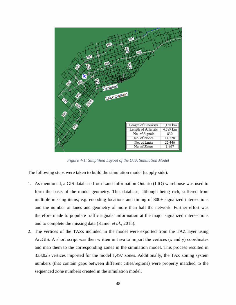
48

Figure 4-1: Simplified Layout of the GTA Simulation Model

The following steps were taken to build the simulation model (supply side):

1. As mentioned, a GIS database from Land Information Ontario (LIO) warehouse was used to

form the basis of the model geometry. This database, although being rich, suffered from

multiple missing items; e.g. encoding locations and timing of 800+ signalized intersections

and the number of lanes and geometry of more than half the network. Further effort was

therefore made to populate traffic signals’ information at the major signalized intersections

and to complete the missing data (Kamel et al., 2015).

2. The vertices of the TAZs included in the model were exported from the TAZ layer using

ArcGIS. A short script was then written in Java to import the vertices (x and y) coordinates

and map them to the corresponding zones in the simulation model. This process resulted in

333,025 vertices imported for the model 1,497 zones. Additionally, the TAZ zoning system

numbers (that contain gaps between different cities/regions) were properly matched to the

sequenced zone numbers created in the simulation model.

49

3. Unlike the centroid-connector method used in planning models, vehicles in DynusT are

generated and dissipated through generation links and destination nodes, respectively,

specified for each TAZ in the model. The traffic released from generation links is distributed

across the road segments proportional to their capacity and the length. The generation links

and destination nodes were carefully created not to be part of the freeway system across the

GTA. This is because trips normally start/end at parking lots, parking garages, residential

areas, etc. but not along freeways.

4. As described before, the AMS model used in DynusT moves the vehicles based on the

fundamental traffic flow diagrams. DynusT uses modified (single- and two-regime) versions

of the Greenshield traffic flow model to construct the speed-density functions for different

road segments (e.g. freeway, collector, on- and off-ramps, etc.), according to their speed

limits and to the model parameters specified for each category. The model parameters were

calibrated to attain the best fit between the simulated and observed speed-density curves.

Further details of the parameter calibration process are provided in Section 4.3.

4.2. Demand Modelling

The time-dependent OD matrices used as input for the simulation model were extracted from the

2011 TTS data survey, after applying the reported expansion factors to cover the total demand in

the survey area. The demand extracted includes all auto (SOV, HOV, taxi passenger, and

motorcycles) morning trips from 6:00 to 10:30 am generated every 15 minutes. The majority of

home-based work trips in the GTA – on which we focus in this study – were observed to occur

during this time period (Sasic and Habib, 2013). Although the core demand entered into the

model corresponds to 4.5 hours, the simulation is conducted for a 6-hour period to account for

warming up the network and draining the demand at the end of the simulation.

To reflect the sheer size of the input demand data, an OD matrix with 2.25 million cells (1497 x

1497 OD combinations) is generated every 15 minutes over the 6:00 to 10:30 am period,

resulting in more than 40 million OD cell records that are fed into the simulation model. During

this period, around 2 million trips traverse the area modelled in the GTA network; their

individual traces are stored on a minute-per-minute basis.

50

Despite their unquestionable impact on traffic conditions, truck demand and transit on-street

units (e.g. buses and street cars) are not included in the input demand considered. . This is

primarily due to the absence of their relevant data in the TTS survey from which the input

demand was extracted. Additionally, the DTA simulation software used does not include a transit

assignment model to simulate/assign transit units in the network. However, the absence of trucks

and transit units in the model was compensated for by adjusting the demand of some ODs during

the model calibration process (Section 4.3). This was applied to ODs feeding corridors where

loop detector readings exceeded simulated traffic (probably due to shortage in the input demand).

It is also important to emphasize that this study focuses on the morning peak period of traffic,

during which truck demand is relatively low (Roorda et al., 2010).

4.2.1. Demand-related Issues

4.2.1.1. Demand Smoothing

The shorter the time intervals by which OD matrices are generated from the travel survey data,

the more accurate the simulation model can capture traffic flow and speed dynamics, especially

in the congested peak periods. However, this comes at the expense of the size and processing

time of the input demand data. Additionally, it might lead to inaccurate simulation results

depending on the quality and richness of the collected survey data.

As mentioned, 15 minute-wide OD demand matrices were used as input to the simulation model.

A flip-flopping pattern was, however, observed in the number of trips generated over the

successive (15 minutes) time intervals. More specifically, the number of trips generated at

quarter-hours (6:15, 6:45, 7:15 and so on) falls behind those generated at half-hours (6:00, 6:30,

7:00 and so on), respectively. This is mostly due to the fact that survey respondents have a

tendency to report their trip start times on a half-hour basis, rather than quarter-hours. In other

words, the majority of trips started between 7:00 and 7:30 am (say) were reported to have started

at 7:00 am, although some of them might have started at (or after) 7:15 am in reality. To resolve

this issue, the OD matrices were filtered through a mathematical procedure, denoted as a moving

average, to generate a smooth demand curve while maintaining the same total number of trips

(Kamel et al., 2015).

51

4.2.1.2. Adding Background Demand

Being a centre for business, finance, education, and culture, Toronto attracts much traffic that

passes through the GTA region but starts and/or ends outside of it. This extra traffic is referred to

hereafter as the ‘background demand’. It has three types: 1) from outside the GTA to the inside,

2) from the GTA to the outside, or 3) from and to zones outside the GTA but passing through

some routes within the network. Ignoring this background demand might underestimate the

amount of traffic flowing on the network main corridors.

To handle this issue, a model of the Greater Toronto and Hamilton Area (GTHA) was simulated

to identify the background trips (fulfilling any of the above three criteria) and add them at the

proper time-intervals to the corresponding input OD cells of the GTA network (shown on the

right-hand side of Figure 4-2). More specifically, the simulation results of the large GTHA

network (shown on the left-hand side of Figure 4-2) were analyzed by tracing the paths of the

spotted background trips and identifying the following:

1. The trip origin and destination zones within the GTA: For types 1 and 3 trips, the origin

zone is modified to be the GTA boundary zone through which the trip traverses inwards

to the GTA network. For types 2 and 3 trips, the destination zone is modified to be the

GTA boundary zone through which the trip traverses outwards from the GTA network.

Otherwise, the origin or destination zones remain unchanged.

2. The trip modified start time: For types 1 and 3 trips, the start time is modified to be the

time at which the trip reaches the boundary of the GTA network (identified from the

output of the GTHA simulation model). The modified time is obviously larger than the

actual trip start time due to the time elapsed from the beginning of the trip until it reaches

the GTA boundary. On the other hand, the start times of type 2 trips are not changed.

Following the described procedure, around 260,000 trips were added to the original (GTA only)

demand, resulting in a total of 2 million trips traversing the GTA simulation model in the

morning period. In other words, the background demand constitutes 13% of the total demand

entered into the GTA simulation model used here. Figure 4-3 shows the total smoothed demand

of the GTA (at each 15 minute interval) during the morning period, before and after including

the background trips.

52

Figure 4-2: Background Demand Illustrating Diagram

Figure 4-3: GTA Total Demand Profile (Kamel et al., 2015)

53

4.2.2. Demand Input Modes

In this study, two modes of releasing traffic demand into the simulation model are utilized: 1)

typical OD demand matrix, and 2) vehicle-by-vehicle input with detailed start time and path

information. Initially, the vehicles in the network are simulated from the input time-dependent

OD matrices, extracted from travel survey data, over the simulation horizon. After a DynusT run

from OD demand matrix mode converges to UE, information of the simulated vehicles (e.g.,

vehicle ID, start time, and origin and destination zones) is listed in output files. DynusT can use

this vehicle-by-vehicle output information as input for alternative scenarios.

The advantage of using the second input mode is having an apples-to-apples comparison

between the base-case scenario and a variety of other scenarios with the same input vehicles. In

other words, the vehicle-by-vehicle input mode removes the possibility of variability in

simulation results stemming from different vehicle input. As described, the second mode is based

on the completion and output of a DynusT run from the OD demand matrix mode. Accordingly,

in order to apply the departure time choice model to capture the impact of variable tolling on the

start times of specific vehicles in the network, the base-case network is re-simulated (after a

complete run with OD demand mode) with the imposed tolling scenarios using the detailed

vehicle-by-vehicle input mode.

4.3. Simulation Model Calibration and Validation

Sections 4.1 and 4.2 have indicated the amount and diversity of the data required to develop the

supply and demand sides of the simulation model. Dealing with the diversity and size of data

sources to build the simulation model was a challenging task. However, more challenging was

the calibration process conducted after the model was built, for validating its base-case output

and therefore being able to use it for new policy assessment. Clearly, the larger the size of the

model and its associated input data, the more factors affecting the accuracy of its output;

consequently, the more complicated and multidimensional the calibration process.

The calibration process consisted of: 1) proper choice of model parameters, e.g. value of time

(VOT), traffic flow model parameters, and freeway bias factor that controls travellers’ perception

bias towards freeway travel time; and 2) handling issues emerging from possible input data

54

inaccuracies, e.g. bias in survey responses and imprecise GIS database information. The

calibrated model was then validated by plotting – i.e., comparing – the simulated traffic volumes

and speeds at 177 locations (over Highways 400, 401, 403, 404, QEW, the Gardiner expressway,

and the Lakeshore Boulevard) against their corresponding observed values collected from loop

detector readings. Additionally, the GEH statistic was utilized as an evaluation criterion for the

simulated volumes in the GTA model (Kamel et al., 2015), as will be detailed later on.

The efforts exerted to correct the input demand inaccuracies include demand smoothing to

resolve the observed flip-flopping pattern (as described in Section 4.2.1) and increasing or

decreasing the demand of some OD pairs, at specific time-intervals, to match traffic on the key

corridors these OD’s affect. A direct impact of the latter step is to compensate for the absence of

trucks and transit units in the input demand, as mentioned earlier. On the supply side, the

geometry (e.g. number of lanes) and speed limits of highways and major arterials and ramps

were carefully checked and adjusted.

Further details of the VOT and traffic flow model parameters selected, the GEH statistic used to

measure the calibrated model accuracy, and the DUE convergence of the simulation model are

described next.

4.3.1. Value of Time (VOT) and Freeway Bias Factor

The objective of DUE assignment is to estimate traffic distribution among alternative routes, for

each OD pair and assignment interval, by equilibrating the generalized cost of all routes. The

generalized cost consists of the actual travel time and the equivalent travel time of tolls charged

on the route (if any) based on the VOT specified (Chiu et al., 2008). In this context, VOT

represents the amount of money the trip maker is willing to pay to save a unit travel time. VOT

varies across individuals because of their different socioeconomic characteristics, attitudes, trip

purposes, and latent preferences (Lu et al., 2006). Hence, some trip makers take slower paths to

avoid tolls, whereas others choose toll roads to save time.

There is no consensus on a unique VOT for the GTA region. Various economic factors affect the

value of this parameter; e.g. time of day choice, labour supply, taxation, activity scheduling,

intra-household time allocation, and out-of-office productivity (Small, 2012).

55

Habib and Weiss (2014) investigated the temporal evolution of commuting mode choice

preference structures using three datasets of TTS surveys collected over a 10-year period. From

the empirical models obtained, the authors estimated the VOT as the ratio of the coefficients of

in-vehicle-travel-time and travel cost variables. The average VOT, among different occupation

groups, was found to be 8.37 $/hr, in 2006 Canadian dollars. Accounting for Canadian inflation

rates from 2006–2015, this value is equivalent to 10 $/hr in 2015 Canadian dollars (Worldwide

Inflation Data, 2015). In a more recent study, Zohreh et al. (2016) investigated commuting mode

choices using a fused SP and RP dataset collected in the GTHA. The subjective value of in-

vehicle-travel-time saving was directly estimated in the systematic utility function of the model.

It was found to vary from 14.5–19.5 $/hr. According to findings of both studies, the average

VOT used in this study for the GTA simulation model is 15 $/hr.

The traffic assignment software used allows for only single-user class with single VOT.

According to Lu et al. (2006), considering multiclass traffic assignment (i.e., considering

heterogeneity in VOT in route choice) is generally challenging in large-scale simulation models

due to computational efficiency and solution storing space issues. The findings of the same study

on a relatively small network (180 nodes, 445 links, and 13 zones) show that using a single VOT

in the model (as opposed to discrete or continuous range of VOT) might bring biased

estimation/prediction of network performance. This is due to overestimating or underestimating

the toll-road usage when the toll charged is relatively low or high, respectively. This possible

bias is, however, alleviated in the current study as follows:

1. The integration of the toll optimization module into the developed congestion pricing system

aims at determining the optimal (i.e., moderate) toll structures triggering traffic re-

distribution over time and space that bring the best network performance. It can be concluded

from the findings of Lu et al. (2006) that if toll levels are moderate (i.e., neither low nor

high), the prediction of network performance will probably be consistent under different

VOT assumptions: single, discrete range, or continuous range. Accordingly, it is expected to

obtain un-biased prediction of network performance under the optimized toll charges.

2. The departure time choice model integrated in the optimal congestion pricing system

considers users’ heterogeneity in values of (early or late) schedule delay and desired arrival

56

time, as will be illustrated in detail in Chapter 5. In other words, drivers’ heterogeneity is

considered in the departure time choice level.

The ‘Freeway Bias Factor’ is another parameter that was adjusted in the calibration process of

the simulation model. This controls the traveller's perception bias towards freeway travel time

and can take values between 0–100. The value selected for this parameter (to obtain realistic

congestion on freeways) is 10; i.e., drivers will perceive the freeway link travel time to be

shorter by 10%.

4.3.2. Traffic Flow Model Parameters

As mentioned earlier, vehicle movements in DynusT are simulated through the Anisotropic

Mesoscopic Simulation (AMS) concept, which assumes that a vehicle’s speed depends on the

density of the vehicles ahead of it in the same lane or adjacent lanes, in what is referred to as the

speed influencing region (SIR). The length of the SIR is one of the parameters that may be

controlled/calibrated in DynusT. The typical value assigned for this parameter, and used here, is

around 240 m. The relationship between the speed and the density is governed by single- and

two-regime traffic flow models, defined in Equations (4-1) and (4-2), respectively. In the two-

regime model, the speed (v) equals the free-flow speed (vf) for densities less than the breakpoint

density (kbp); whereas it follows a modified Greenshield equation for higher densities where

other parameters – such as the minimum speed (v0), the jam density (kj), and the shape term (α) –

affect the relationship (Chiu et al., 2010). The single-regime model is a special case of the two-

regime model, where the breakpoint density equals zero, as can be inferred from the two

equations.

(4-1)

(4-2)

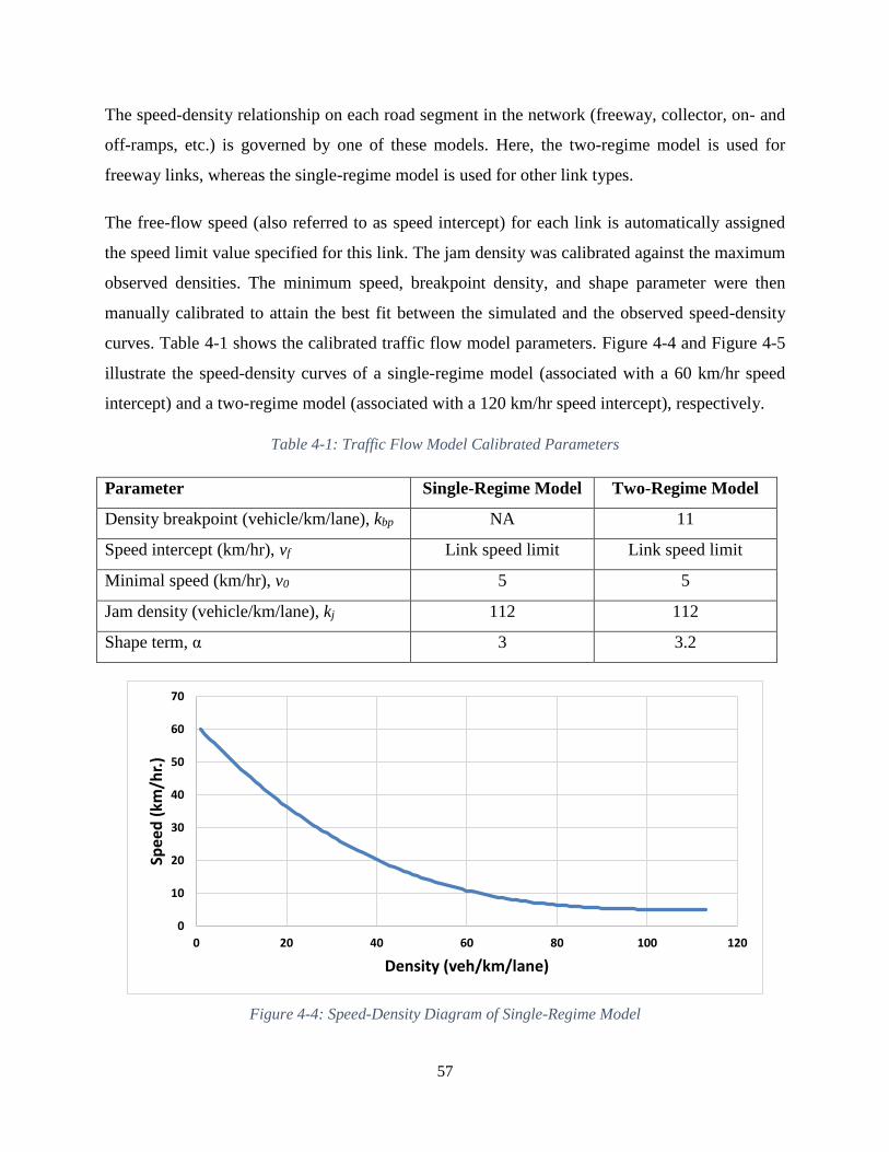
57

The speed-density relationship on each road segment in the network (freeway, collector, on- and

off-ramps, etc.) is governed by one of these models. Here, the two-regime model is used for

freeway links, whereas the single-regime model is used for other link types.

The free-flow speed (also referred to as speed intercept) for each link is automatically assigned

the speed limit value specified for this link. The jam density was calibrated against the maximum

observed densities. The minimum speed, breakpoint density, and shape parameter were then

manually calibrated to attain the best fit between the simulated and the observed speed-density

curves. Table 4-1 shows the calibrated traffic flow model parameters. Figure 4-4 and Figure 4-5

illustrate the speed-density curves of a single-regime model (associated with a 60 km/hr speed

intercept) and a two-regime model (associated with a 120 km/hr speed intercept), respectively.

Table 4-1: Traffic Flow Model Calibrated Parameters

Parameter Single-Regime Model Two-Regime Model

Density breakpoint (vehicle/km/lane), kbp NA 11

Speed intercept (km/hr), vf Link speed limit Link speed limit

Minimal speed (km/hr), v0 5 5

Jam density (vehicle/km/lane), kj 112 112

Shape term, α 3 3.2

0

10

20

30

40

50

60

70

0 20 40 60 80 100 120

Spee

d (

km/h

r.)

Density (veh/km/lane)

Figure 4-4: Speed-Density Diagram of Single-Regime Model

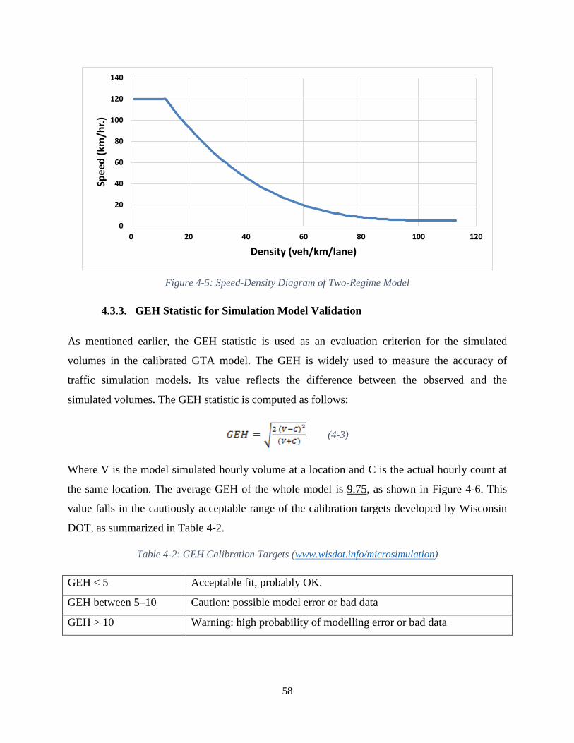
58

0

20

40

60

80

100

120

140

0 20 40 60 80 100 120

Spee

d (

km/h

r.)

Density (veh/km/lane)

Figure 4-5: Speed-Density Diagram of Two-Regime Model

4.3.3. GEH Statistic for Simulation Model Validation

As mentioned earlier, the GEH statistic is used as an evaluation criterion for the simulated

volumes in the calibrated GTA model. The GEH is widely used to measure the accuracy of

traffic simulation models. Its value reflects the difference between the observed and the

simulated volumes. The GEH statistic is computed as follows:

(4-3)

Where V is the model simulated hourly volume at a location and C is the actual hourly count at

the same location. The average GEH of the whole model is 9.75, as shown in Figure 4-6. This

value falls in the cautiously acceptable range of the calibration targets developed by Wisconsin

DOT, as summarized in Table 4-2.

Table 4-2: GEH Calibration Targets (www.wisdot.info/microsimulation)

GEH < 5 Acceptable fit, probably OK.

GEH between 5–10 Caution: possible model error or bad data

GEH > 10 Warning: high probability of modelling error or bad data

59

The best attained GEH of 9.75 was therefore accepted with three factors in mind: (1) the sheer

size of the regional network, (2) the large number of loop detector stations and the inevitable

variability in the quality of the loop detector data used in the calibration process and (3) possible

inaccuracies in TTS data (from which demand was extracted) resulting from respondents’ biases.

Figure 4-6: Scatterplot of the Observed and Simulated Hourly Volumes (Kamel et al., 2015)

4.3.4. Simulation Model DUE Convergence and Relative Gap

As mentioned in Chapter 3, the convergence criterion used for the traffic assignment model is

referred to as the Relative GAP (RG). The RG at each iteration represents the relative difference

between total travel times experienced for all users over their assigned paths (resulting from this

specific iteration) and the total travel times of shortest-path DUE conditions. The difference is

relative to the combined total shortest travel times for all the demand. The RG reflects how close

the assignment solution (at each iteration) is to the target User Equilibrium (UE) network

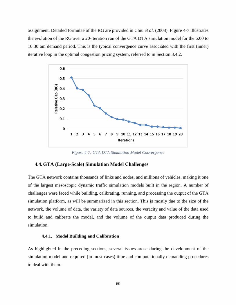
60

assignment. Detailed formulae of the RG are provided in Chiu et al. (2008). Figure 4-7 illustrates

the evolution of the RG over a 20-iteration run of the GTA DTA simulation model for the 6:00 to

10:30 am demand period. This is the typical convergence curve associated with the first (inner)

iterative loop in the optimal congestion pricing system, referred to in Section 3.4.2.

0

0.1

0.2

0.3

0.4

0.5

0.6

1 2 3 4 5 6 7 8 9 10 11 12 13 14 15 16 17 18 19 20

Rel

ativ

e G

ap (

RG

)

Iterations

Figure 4-7: GTA DTA Simulation Model Convergence

4.4. GTA (Large-Scale) Simulation Model Challenges

The GTA network contains thousands of links and nodes, and millions of vehicles, making it one

of the largest mesoscopic dynamic traffic simulation models built in the region. A number of

challenges were faced while building, calibrating, running, and processing the output of the GTA

simulation platform, as will be summarized in this section. This is mostly due to the size of the

network, the volume of data, the variety of data sources, the veracity and value of the data used

to build and calibrate the model, and the volume of the output data produced during the

simulation.

4.4.1. Model Building and Calibration

As highlighted in the preceding sections, several issues arose during the development of the

simulation model and required (in most cases) time and computationally demanding procedures

to deal with them.

61

On the demand side, importing around 2.25 million OD cells to the model every 15 minutes

(over the course of 4.5 hours) involved several processing hours of the OD matrices extracted

from TTS diaries. This is due to the specific input format required by the simulation software,

e.g. all matrix cells should be provided, even if they contain zero records, in addition to the

effort/time taken to match the GTA TAZ zoning numbers to the sequenced numbering created

and used in the simulation model. Also, as described earlier, a mathematical procedure was

applied to generate a smooth demand pattern and to correct the flip-flopping phenomenon

observed at quarter-hours, possibly due to survey respondents’ bias. Additionally, the

background demand (that starts and/or ends outside the GTA region but passes through it) was

identified and added to the GTA demand at proper time intervals and OD cells by processing the

trajectories of around 2.2 million vehicles simulated in a larger model of the GTHA region.

Moreover, the demand of some OD pairs at specific time intervals was adjusted to match

congestion on the key corridors that these ODs affect. This was performed by analyzing the paths

of the trips travelling through those corridors to obtain their ODs and hence adjusting those that

contribute highly to the corridor traffic.

On the network geometry side, the GIS database played a key role in forming the basis of the

model geometry; however, it suffered from several missing items. Accordingly, the geometry

(e.g. number of lanes) and speed limits of highways and major arterials and ramps all over the

network were carefully checked and adjusted. Another non-trivial task was to allocate (non-

freeway) generation links and destination nodes for each of the model 1497 TAZs. Although the

allocation process was automated, several zones had to be re-processed individually upon

receiving simulation errors related to releasing their demand (e.g., a dead-end link might be

assigned by mistake as a generation link).

On the model calibration side, the process was multidimensional and time-consuming due to the

sheer size of the model and the numerous factors affecting the output simulation results, as

illustrated in the previous section. Moreover, the loop detectors’ raw data available contain

millions of daily records over several years. Therefore, these datasets had to be inspected to

extract traffic speeds and volumes that could be used for model calibration and validation. Due to

the variations and seasonality of the observed data, a wide range of weekdays (Tuesday,

Wednesday, and Thursday) across several months (September, October, and November), over

62

the period from 2010–2012 (during which TTS survey data were collected), were considered in

the calibration process. Special procedures, detailed in Kamel et al. (2015), were followed to

identify the defective loop detectors to be excluded – based on their reported data – and the

correctness of the counts obtained from non-defective (i.e., accepted) loop detectors.

4.4.2. Model Execution: Required Resources and Runtime

The model runtime is generally affected by the following factors: network size, demand size (i.e.,

number of OD cells and demand intervals), number of computer processors allocated to the

simulation model, and number of iterations specified for DUE.

The memory usage fluctuates during model execution depending on the task being performed

(viz. assignment, simulation, writing vehicle information into files, etc.). In the GTA simulation

model, the maximum memory usage reaches around 13.5 GB. This high memory consumption is

due to the sheer size of the model and the associated massive computations and storage-space

requirements during the simulations.

On an i7 Machine with 16 GB of RAM, the DTA run-time of the GTA simulation model until

convergence (using 20 iterations) is around 7.5 hours. The associated RG curve, representing the

1st level of convergence (i.e., route choice convergence) in the optimal congestion pricing

system, is shown in Figure 4-7. As clarified in the description of the optimal congestion pricing

system (provided in Section 3.4), the GTA simulation model is run several times in sequence

with the departure time choice model – under each tolling scenario tested – until the 2nd level of

convergence (i.e., departure time convergence) is reached. Moreover, the hybrid testbed (i.e., the

combined departure time choice and DTA simulation models) is run several times to test

different tolling scenarios generated by the optimization algorithm until the 3rd level of

convergence (i.e., toll structure convergence) is reached. Therefore, running a single full-price

optimization scenario would take several weeks if it is executed in a serial mode using a single

high-end PC (in terms of memory and CPUs).

The required resources and runtimes were obstacles against full system implementation. These

challenges made use of a parallel high-performance cluster an urgent need to run the full system

in a reasonable time. Running the system in parallel mode entailed significant effort to set up and

63

configure parallel computer nodes for the proper communication and task distribution among

them, as will be described in detail in Chapter 7.

4.4.3. Processing Model Output

The simulation modelling platform generates output statistics at different levels: network-wide,

link-based, and trip-based. Output statistics vary in volume and frequency of generation. On the

network-level, total travel times and total trip distances are single values, produced once for the

entire network at the end of the simulation. On the other hand, the number of vehicles generated,

inside and leaving the network, is released every minute throughout the simulation. On the link-

level, average speeds, densities, and queue lengths are reported every minute for each single link.

This results in about 40 million readings for traffic data of the morning period simulated in the

GTA. On the trip-level, detailed vehicle trajectory data are provided for each vehicle in the

simulation; e.g. origin node, destination node, start time, nodes traversed, times spent on each

link, and total trip time. The vehicles’ path and time information is updated almost every second;

this process generates more than 17 million node-arrival time pairs each hour.

The large volume and frequency of the generated traffic data posed serious challenges to extract

meaningful information from this huge dataset. Data processing and analytical techniques were

used to deal with the raw output data of the simulation model and to extract useful information

that could be used to analyze the network performance – at various levels – under pricing

policies, and therefore make informative pricing-related decisions (e.g. tolling periods, locations,

levels, etc.).

This chapter has emphasized the efforts exerted to build, calibrate, and validate a large-scale

DTA simulation model for the GTA based on the most recent available demand data, GTA TAZs

system, network geometry information, and loop-detector feeds. In fact, using this simulation

model – integrated with the other system components – for optimal toll determination and

realistic estimation of drivers’ behavioural responses to pricing network-wide, is one of the

major contributions of this study.

64

5. The Econometric Model for Departure time Choice in the GTA:

Retrofitting and Integration with the DTA Simulation Model

The integration of an econometric departure time choice model into the proposed optimal

congestion pricing system is important to assess the differential impact of pricing scenarios on

the departure time choice of distinct drivers. The departure time shift due to time-dependent tolls

is one of the key travel behaviour changes to be expected, which can induce significant benefits

to motorists and the system overall. It not only relieves the infrastructure from overuse,

congestion and delays, but does so in a manner that is proportional to the problem itself; i.e.

congestion, when and where it occurs.

This chapter describes the details of the econometric model used to model departure time choice

in the proposed optimal congestion pricing system. The chapter starts with an introduction to the

different approaches to simulate departure time changes. An overview is then given to the

departure time choice set formulation and the original variables used in the model utility

functions and scale parameters. The extensions and assumptions to incorporate schedule-delay

and toll cost in the model and to re-calibrate the associated parameters are then discussed. The

steps followed for the preparation/estimation of the data required by the model are then

presented. After that, the model implementation details to simulate commuters’ departure time

choices and the convergence criterion of the model output are described. Finally, the model base-

case validation results are illustrated.

5.1. Simulating Departure Time Change Approaches

Several approaches can be followed to simulate drivers’ departure time along with route changes

within a traffic simulation environment. The most simple, yet non-realistic, approach is to induce

random perturbation of trip start times throughout the simulation, based on a certain pre-set

probability, as in Balmer et al. (2008). This approach is easy to implement and is not

computationally demanding. However, the stochastic mutations might bring unrealistic start

times (e.g., a work trip starting at 2:00 am). Additionally, the changes in start time are not

directly affected by the policies introduced (like time-dependent congestion pricing).

65

Another approach, followed by Lu et al. (2006), involves joint departure time and route-choice

algorithms – implemented iteratively until equilibrium – based on a set of trip attributes that

include travel time, out-of-pocket cost, and schedule-delay cost. This approach has the advantage

of realistically modelling the joint nature of both departure time and route choices within a

simulation environment. However, it cannot be handled in a large network setting within the

limits of practical computational capabilities. Additionally, it does not consider the impact of

driver-related attributes (e.g. personal and socio-economic characteristics) on the choice-making

process.

A third approach, followed here, is through integrating an econometric behavioural departure

time choice model (that considers both trip and driver attributes) into a large-scale traffic

assignment simulation model. This provides a computationally tractable tool to estimate

departure time and route choice responses to traffic management policies that affect travel times

and costs, in a large-scale setting. The problem with this approach is the underlying assumption

that departure time and route choices are made sequentially (rather than jointly). However, this is

compensated for here by iterating and feeding back between departure time and route choices

until both choices reach equilibrium.

5.2. Overview of the Departure Time Choice Model Used

As briefly mentioned in Chapter 3, this study extends a recently developed model (Sasic and

Habib, 2013) at the University of Toronto that describes departure time choice in the GTHA. The

key challenges in departure time choice modelling are accurately representing the continuous

nature of time while allowing a comparison of non-adjacent departure time slots and capturing

the choice captivity to specific time slots. The model combines a heteroskedastic Generalized

Extreme Value (Het-GEV) structure with overlapping choice sets that account for alternative

choice correlation and choice captivity. Overlapping choice sets also allow for the continuous

nature of departure time choices.

The choice probabilities are expressed as the probability of a choice set being selected multiplied

by the conditional probability of selecting the choice from within the choice set. The probability

that a choice set is selected depends on the expected maximum utility of the choice alternatives

within the set. The random utility for any alternative is defined as a systematic and a random

66

component, where the joint density of all random components is distributed according to the

extreme value distribution.

Two types of scale parameters are introduced in this model. These are the root scale parameter

and the nest scale parameter of a particular choice set. Moreover, the modelling framework uses

a scale parameterization approach to capture heteroskedasticity in departure time choices. This

approach also captures heterogeneity in users’ departure time choice responses to variations in

trip-related attributes (e.g. travel time and cost) at each choice interval. The model was

developed and calibrated in the original study using the Transportation Tomorrow travel Survey

(TTS) of 2006.

In this study, effort has been devoted to calibrating/retrofitting the Sasic and Habib (2013) model

to meet current research needs. The model was retrofitted using the latest TTS survey of 2011

(DMG, 2015). Additionally, schedule-delay and toll cost components were incorporated in the

model variables, and their associated parameters were recalibrated accordingly. It is noteworthy

that the TTS survey does not have data about tolling or users’ response to such cost. Therefore, a

model for capturing the impact of tolling on travellers’ behaviour cannot be estimated directly

from the TTS data, hence the need to retrofit the above model. Perhaps in the future the impact

of tolling on travel behaviour could be directly estimated via stated preference surveys, but this is

beyond the scope of this study.

5.3. Original Model Formulation

5.3.1. Choice Set Formulation

The datasets from the 2006 TTS survey (DMG, 2015) were used for the empirical model of

departure time choices of home-based commuting (i.e. home to work or school) trips in the

Greater Toronto and Hamilton Area (GTHA) (Sasic and Habib, 2013). The datasets from the

latest 2011 TTS survey are used here to retrofit the 2006 model for 2011 conditions, as will be

explained in the next section. In this model, departure time is represented as nine (30 min)

discrete time intervals – lying within eight choice sets – that span the morning peak (when the

majority of home-based work trips occur), as shown in Figure 5-1. The reason a 30 min

bandwidth is used is that it was found to carry the minimum level of detail required to represent

67

variability in the departure time choice distribution. Shorter intervals resulted in a lack of

observations for a significant number of alternative departure time options.

The choice framework is shown in Figure 5-1. This framework resembles the decision making

process, where an individual chooses his/her departure time within a specific range (portion) of

the day. The overlapping choice sets allow individual choice alternatives to be in multiple choice

sets, and hence accommodate the latent choice set approach within the choice probability

calculation. In other words, the probability that an individual chooses to depart from home to

work during some interval is defined as the weighted sum of the probability of choosing this

time-interval over the one preceding it, and the probability of choosing this time-interval over the

one following it. Moreover, the probability of choosing some departure time interval is affected

by explanatory variables, as well as the scale parameters that explain additional choice

heterogeneity.

Figure 5-1: Departure Time Choice Framework in the Het-GEV Model, (Sasic and Habib, 2013)

5.3.2. Model Variables

Two types of explanatory variables exist in this model, in the systematic utility functions and the

root and nest scale parameters; namely, 1) commuters’ personal and socio-economic attributes;

and 2) transportation level-of-service (LOS) attributes corresponding to alternative departure

time segments. Commuter attributes include: work duration, occupation category (general office,

manufacturing, or professional), gender, job status (full- or part-time), and age category. Level-

68

of-service attributes include travel time, travel distance, and travel cost corresponding to each

departure time segment. Table 5-1 summarizes the model’s original variables defining its

systematic utility functions, root scale parameter, and nest scale parameters. The highlighted

variables in the first column are dummy variables that take 0 or 1 values. Downtown Toronto, in

the study context, involves 18 TAZs bounded by Front Street, Bloor Street, Yonge Street, and

Spadina Avenue. The steps taken to prepare/calculate the model variables corresponding to the

GTA morning commuting trips (considered here) are presented in Section 5.5.

Table 5-1: Departure Time Choice Model Variables (Sasic and Habib, 2013)

Variable Description

Systematic Utility Function:

ASC Alterative Specific Constant

TC Total Cost

IVTT In-Vehicle Travel Time

WD (or SD) Work (or School) Duration

Dest Destination of the trips: downtown Toronto

Occ1 Occupation category: general office

Occ2 Occupation category: manufacturing

Occ3 Occupation category: professional

Root Scale Parameter:

Gen Gender: male

Age1 Less than 25 years old

69

Age2 25–35 years old

Age3 35–45 years old

Job Job status: full-time

TC/TD Total Cost/ Total Distance

IVTT/TD In-Vehicle Travel Time/ Total Distance

Orig Trip origin: downtown Toronto

Dest Trip destination: downtown Toronto

Nest Scale Parameter:

LogDist Logarithm of distance between origin and destination

As mentioned earlier, the modelling framework uses the scale parameterization approach. This is

clear from Table 5-1, where the scale parameters do not take constant values; rather, they vary

according to trip and driver attributes. This approach captures heterogeneity in users’ departure

time choice responses to variations in trip-related attributes (e.g. travel time and cost) at each

choice interval. More specifically, the root scale parameter μR explains the baseline heterogeneity

across the population; the higher the value of μR, the more stable the choices, and vice versa. In

other words, the class of trip makers having low values of μR are choice users, whereas those who

have high values of μR are more captive users. On the other hand, μc is the nest scale parameter

for choice set c. A higher value of μc indicates higher correlation between the shared alternatives

within the nest, and vice versa. The probability of choosing certain alternative j, Pj, is calculated

as follows:

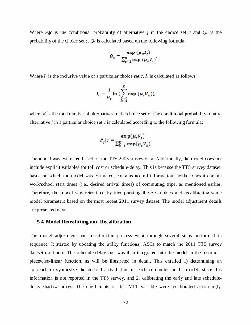
70

Where Pj|c is the conditional probability of alternative j in the choice set c and Qc is the

probability of the choice set c. Qc is calculated based on the following formula:

Where Ic is the inclusive value of a particular choice set c. Ic is calculated as follows:

where K is the total number of alternatives in the choice set c. The conditional probability of any

alternative j in a particular choice set c is calculated according to the following formula:

The model was estimated based on the TTS 2006 survey data. Additionally, the model does not

include explicit variables for toll cost or schedule-delay. This is because the TTS survey dataset,

based on which the model was estimated, contains no toll information; neither does it contain

work/school start times (i.e., desired arrival times) of commuting trips, as mentioned earlier.

Therefore, the model was retrofitted by incorporating these variables and recalibrating some

model parameters based on the most recent 2011 survey dataset. The model adjustment details

are presented next.

5.4. Model Retrofitting and Recalibration

The model adjustment and recalibration process went through several steps performed in

sequence. It started by updating the utility functions’ ASCs to match the 2011 TTS survey

dataset used here. The schedule-delay cost was then integrated into the model in the form of a

piecewise-linear function, as will be illustrated in detail. This entailed 1) determining an

approach to synthesize the desired arrival time of each commuter in the model, since this

information is not reported in the TTS survey, and 2) calibrating the early and late schedule-

delay shadow prices. The coefficients of the IVTT variable were recalibrated accordingly.

71

Finally, the toll cost variable was added to the total cost, and the corresponding toll coefficient

was then calibrated.

As outlined, each step involved calibrating specific parameters in the model. The calibrated

parameters were determined using a factorial design procedure (Cheng, 2013). The objective of

this procedure was to determine the set of parameters that brought the best model base-case

validation results, at the designated step. The validation was performed by implementing the

modified departure time choice model together with the traffic simulation model iteratively until

convergence – i.e., executing the testbed shown in Figure 3-1 – under base-case conditions (i.e.,

without tolling). After convergence, the resulting simulated traffic conditions are compared

against those obtained without applying the departure time choice model. The purpose of

calibration is hence to find the parameters that minimize the absolute error between both

simulated outputs, at all time intervals, for the following measurements:

- number of commuters who choose to depart at each time interval;

- average resulting travel time per km (calculated by averaging the travel time of each

commuter divided by the distance travelled in km, over all commuters departing at each

time interval); and

- average distance travelled.

Intuitively, a perfect (i.e. 100% accurate) departure time choice model should bring identical

demand temporal distribution and hence identical simulated traffic attributes, at base-case

network conditions, to those obtained under the original demand extracted from TTS data

without applying the departure time choice model. The validation details and final results are

presented in Section 5.7.

5.4.1. Alternative Specific Constants (ASCs)

The departure time choice model considers the following: 1) alternative specific constants, 2)

coefficients of variables defining systematic utility functions, 3) coefficients of variables

defining the root scale parameter, and 4) coefficients of variables defining the nest scale

parameters. As a result, the model has 74 statistically significant parameters. The empirical

model was originally estimated based on the 2006 TTS survey. The alternative specific constants

72

(ASCs) were therefore updated to be consistent with the 2011 dataset, according to the following

rule (Train, 2003):

Where Ai is the number of decision-makers in the 2011 population who chose departure time

interval i, and Si is the number of decision-makers in the 2006 population who chose the same

interval. Table 5-2 shows the ASCs before and after adjustment. The updated constants are

proportional to the corresponding shares of drivers in the 2011 dataset – at each time-interval –

yet carrying the behavioural information involved in the originally estimated constants. It can be

noted from the table that the updated ASCs are higher than the original ASCs. This is due to the

fact that the 2011 population, hence shares in different departure time intervals, is larger than

that of 2006.

Table 5-2: Original and New ASCs in the Departure Time Choice Model

Time

Interval

6:00 to

6:30

6:30 to

7:00

7:00 to

7:30

7:30 to

8:00

8:00 to

8:30

8:30 to

9:00

9:00 to

9:30

9:30 to

10:00

10:00 to

10:30

Original

ASCs 0 -0.4508 -0.2099 0.1803 0.3659 0.1143 0.007 -0.3665 1.3054

New

ASCs 1.0010 1.0426 1.4983 2.0899 2.3680 2.2478 2.0469 1.3484 1.7053

5.4.2. Schedule-Delay Cost

The schedule-delay (early or late arrival) cost is intuitively an important factor contributing to

the departure time choice for morning commuting – i.e., work or school – trips (having a specific

desired arrival time). It is crucial to attain the anticipated departure time rescheduling effects of

tolling in accordance with the Bottleneck Model pricing structure adapted here. As mentioned,

this variable is absent from the original model, since the work/school start times (i.e. desired

arrival times) of commuting trips are not reported in the TTS survey. Without schedule-delay

cost, the model would erroneously exaggerate shifting commuting trips to outside the toll period.

73

In other words, the schedule-delay cost is what keeps commuters “anchored” to their desired

arrival times. Accordingly, this schedule-delay variable is added to the travel time variable in the

model.

The schedule-delay cost, cs, used here takes the following formula (Small, 1982):

where β and γ are the shadow prices of early and late arrival delays, respectively. t is the trip start

time, T(t) is the travel time, and td is the desired arrival time.

According to Verhoef (2003), early and late arrival delays are perceived differently by

commuters, and hence have different coefficients (i.e., shadow prices) in the schedule-delay cost

function with a ratio of 1 to 4, respectively. This ratio was further modified in this study during

model validation to be 1 to 2, which better fits the GTA data without underestimating the number

of trips that started at late time intervals due to exaggerated late arrival costs. The modified ratio

denotes that GTA travellers perceive the cost of arriving one hour later than desired twice the

cost of arriving one hour earlier.

5.4.3. Desired Arrival Time

The desired arrival time of a commuter is the time at which the commuter wants to arrive at work

or school; deviations from which imply early or late schedule-delays. Obviously, the existence of

desired arrival times (e.g., work/school start times) for morning commuters is what creates a

peak, as travellers are anchored to their desired arrival times. This results in increased travel

times and long queueing delays around the average desired arrival time, and hence creates the

typical morning traffic peak.

As mentioned before, the desired arrival time information is not reported in the TTS survey; only

actual arrival time (shifted from the desired time by an unrevealed schedule-delay component) is

reported. Accordingly, a desired arrival time value is synthesized for each vehicle in the network

once at the beginning of the simulation, and is kept fixed for the entire system implementation.

Heterogeneity is expected to be observed in desired arrival times within a large-scale application

involving millions of commuters having diverse socioeconomic characteristics, employment

74

categories, and work schedules (as in the GTA). Assuming a single desired arrival time in such a

large-scale model results in an overestimated number of trips starting around this single desired

time, and hence creates an exaggerated simulated morning traffic peak. In other words, a model

making that assumption predicts travel times that climb and fall much quicker than observed

(Hall, 2013). It is therefore important to allow for a continuum of desired arrival times in the

model for the sake of more realistic results.

In Hall (2013), desired arrival times follow a uniform distribution over an interval [ts, te], where

ts and te are the first and last desired arrival times, respectively. These times were determined in

that study based on the start and end times of the period at which the slope of observed travel

time profile is fixed. In another transit-related study (Wahba, 2009), the desired arrival time is

synthesised by first establishing a range of possible desired arrival time values for each

passenger. The lower and upper bounds of that range are obtained by adding the minimum and

maximum travel times, respectively, to the trip start time. The range is then discretized to data

points representing 5-minute increments, one of which is selected randomly to be the passenger

desired arrival time.

In this study, the desired arrival time (td) is randomly generated for each vehicle in the network

following a log-normal distribution. i.e., ln(td) is assumed to have a normal distribution with

parameters μ (mean) and σ (standard deviation). The log-normal distribution is suitable for

random variables that are inherently positive. Additionally, it has a quasi-bell shape that enforces

ascending probabilities for values (i.e., desired arrival times) close to the mean, and vice versa.

Accordingly, it is believed to produce a more realistic distribution of simulated desired arrival

times than following a uniform distribution.

Several values were tested for the mean and standard deviation of this distribution; 8:30 am (i.e.

minute 150 counting from 6:00 am) was ultimately selected as the mean desired arrival time (i.e.

μ = ln(150)) and σ = 0.05 – measured in ln(minute) – was set as the standard deviation. The

selected parameters were found to bring the best validation results among other tested values,

when the integrated departure time and traffic assignment testbed is applied in the base-case.

More specifically, they resulted in the closest output distribution of simulated departure (hence

arrival) times for commuting trips to those obtained in the GTA base-case traffic assignment

simulation results (without applying the departure time choice model). The final validation

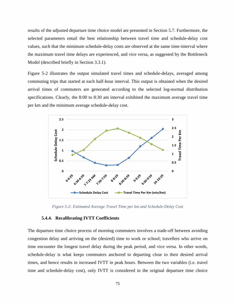
75

results of the adjusted departure time choice model are presented in Section 5.7. Furthermore, the

selected parameters entail the best relationship between travel time and schedule-delay cost

values, such that the minimum schedule-delay costs are observed at the same time-interval where

the maximum travel time delays are experienced, and vice versa, as suggested by the Bottleneck

Model (described briefly in Section 3.3.1).

Figure 5-2 illustrates the output simulated travel times and schedule-delays, averaged among

commuting trips that started at each half-hour interval. This output is obtained when the desired

arrival times of commuters are generated according to the selected log-normal distribution

specifications. Clearly, the 8:00 to 8:30 am interval exhibited the maximum average travel time

per km and the minimum average schedule-delay cost.

0

0.5

1

1.5

2

2.5

3

0

0.5

1

1.5

2

2.5

Trav

el T

ime

Pe

r K

m

Sch

ed

ule

De

lay

Co

st

Schedule Delay Cost Travel Time Per Km (min/km)

Figure 5-2: Estimated Average Travel Time per km and Schedule-Delay Cost

5.4.4. Recalibrating IVTT Coefficients

The departure time choice process of morning commuters involves a trade-off between avoiding

congestion delay and arriving on the (desired) time to work or school; travellers who arrive on

time encounter the longest travel delay during the peak period, and vice versa. In other words,

schedule-delay is what keeps commuters anchored to departing close to their desired arrival

times, and hence results in increased IVTT in peak hours. Between the two variables (i.e. travel

time and schedule-delay cost), only IVTT is considered in the original departure time choice

76

model. The absence of schedule-delay was implicitly compensated for through the estimated

coefficients of IVTT of the original model. More specifically, it can be observed from Figure 5-3

that the original coefficients corresponding to the 6:30 to 8:00 am interval are noticeably larger

than those of the 8:30 to 10:00 am interval. The numerical values are reported in

Table 5-3. This difference attracts more trips to earlier intervals so as to arrive close to their

desired arrival times (e.g. 8–9 am), and hence creates the typical morning traffic peak. In other

words, the differences between the original IVTT coefficients compensate for the

unexplained/missing schedule-delay component.

When the schedule-delay is explicitly incorporated in the departure time choice model, the

summation of both variables (i.e., IVTT and schedule-delay) should naturally bring the typical

bell-shaped distribution of morning traffic demand, without such difference in coefficient values.

Hence, adding schedule-delay while using the original IVTT coefficients will overestimate the

number of trips that start between 6:30 and 8:00 am.

Accordingly, the coefficients of IVTT were recalibrated to avoid biases in model output choices

(as a result of adding schedule-delay costs). The modified parameters are reported in

Table 5-3 and illustrated in Figure 5-3. They were determined using a factorial design procedure,

as described at the beginning of this section.

Table 5-3: Original and Modified Coefficients of IVTT in the Departure Time Choice Model

Time

Interval

6:00 to

6:30

6:30 to

7:00

7:00 to

7:30

7:30 to

8:00

8:00 to

8:30

8:30 to

9:00

9:00 to

9:30

9:30 to

10:00

10:00 to

10:30

Original

Coefficients 0 -0.0107 -0.0087 -0.0149 -0.0196 -0.03 -0.0332 -0.0182 0

Modified

Coefficients -0.015 -0.0187 -0.0167 -0.0249 -0.0196 -0.015 -0.0102 -0.0082 -0.005

77

-0.035

-0.03

-0.025

-0.02

-0.015

-0.01

-0.005

0

Original Time Coefficients Modified Time Coefficients

Figure 5-3: Original vs. Modified IVTT Coefficients

It can be noted from Figure 5-3 that the modified coefficients of the 6:00 to 9:00 am intervals

have relatively close values, compared to the original coefficients. This was expected, as

explained above. However, the modified coefficients obtained for the last three intervals are

relatively higher than the remainder. Other lower coefficients tested at those late intervals

underestimated the number of trips started at them, mostly due the high values of late schedule-

delay costs, indicated in Figure 5-2. Intuitively, the more comprehensive the overall cost function

used in the model (IVTT, schedule-delay, travel distance, fuel cost, tolls, etc.), the better it can

explain the departure time choice behaviour, and hence the fewer differences between the cost

coefficients among various intervals.

5.4.5. Toll Cost

As can be observed from Table 5-1, the model does not include an explicit variable for the toll

cost. This is because the TTS survey dataset contains no toll information to assist in the

coefficient estimation of such parameter. For the sake of variable pricing policy testing in this

study, the imposed tolls are added to the travel cost variable. The coefficient of the inserted toll

variable (in the utility of each departure time choice) is set such that the ratio between the

coefficients of in-vehicle-travel-time (IVTT) and toll variables is compatible with the average

VOT used in the DTA simulation model of $15/hr (indicated in Section 4.3.1).

78

It should be noted that forecasting the impact of hypothetical transportation demand management

strategies based on revealed preference (RP) model parameters might underestimate the impact

of these policies (Habib et al., 2013). In other words, using the auto cost parameter might not be

ideally suited for tolls. This is due to the fact that drivers – to some extent – may not be very

elastic to increases in travel time and basic costs (e.g. maintenance, fuel, etc.); however, they

may react more clearly to changes in parking cost and road charges (i.e., out-of-pocket money),

as it is something they can avoid.

Nevertheless, adding the toll cost to the travel cost variable is expected to give an approximate

estimation of drivers’ behavioural responses to variable pricing. More realistic modelling of

commuters’ responses to pricing in the GTA might be achieved by re-estimating the departure

time choice model based on stated preference (SP) data surveys incorporating toll information, in

addition to the existing revealed preference information in the TTS surveys, which is beyond the

scope of this study and could be undertaken in future work.

The departure time choice model is applied to individual commuters (iteratively and sequentially

with the traffic simulation model) both during the model recalibration/validation phase and

ultimately during optimal congestion pricing policy determination and evaluation. Applying the

model requires providing it with certain personal and trip-related attributes. The next section

presents the procedure followed here to prepare the data necessary to apply the model.

5.5. Model Input Data Preparation

As highlighted in Section 5.3, two types of variables are required by the departure time choice

model: 1) commuters’ personal and socio-economic attributes; and 2) transportation level-of-

service (LOS) attributes corresponding to alternative departure time segments. Commuter

attributes include: work duration, occupation category (general office, manufacturing, or

professional), gender, job status (full- or part-time), and age category. Level-of-service attributes

involve travel time, travel distance, and travel cost corresponding to each departure time

segment. It should be mentioned that the departure time choice model is only applied to

commuting trips (representing the majority of morning trips) for which the original model was

estimated. Hence, route choice is assumed to be the only choice non-commuting trips have to

respond to pricing; it is modelled through the DTA simulator. We believe that this assumption

79

should not create much bias in the overall measured effect, because only a fraction of travellers

typically respond to a toll or other shock by changing departure time. A lack of response from

non-commuters could be compensated for by a more-than-proportional response from

commuters, so that the overall response is similar to a case in which all travellers are flexible.

This section provides the preparation details of both input data classes required for applying the

model to the GTA.

5.5.1. Personal and Socio-Economic Attributes

As clarified earlier, the departure time choice model used here was estimated for morning

commuting (home to work or school) trips in the GTHA, which constitute the majority of

morning trips made during peak hours. Accordingly, the model is applied only to the commuting

trips simulated in the GTA DTA model.

This section presents our efforts to 1) extract the records of the original and background

commuting trips – considered here – from the TTS datasets and to prepare the necessary driver-

related attributes required by the departure time choice model, and 2) design a criterion to

determine whether certain trips in the model are commuting, and properly extract their attributes

(from the database prepared in the first step) based on their OD and start time interval.

5.5.1.1. Preparing Driver-related Attribute ‘Database’ for Commuting Trips

in the GTA Model

The purpose of this step is to prepare a database of the personal and socio-economic attributes,

required by the departure time choice model, for all (original and background) commuting trips

simulated in the GTA model. The database records are extracted from the TTS 2011 survey

datasets. Further processing and calculations are performed on the ‘raw’ survey data to prepare

the necessary attributes required by the model, reported in Table 5-1. The database is constructed

through the following steps:

– Extract all auto (SOV, HOV, taxi passenger, and motorcycles), morning (started from 6:00 to

10:30 am), commuting (ending at work or school) trips – from the TTS datasets – starting

and/or ending at a GTA zone.

– Extract and link the person-related characteristics to the attributes of each filtered trip.

80

– Calculate the dummy variables required by the model (Occ1, Occ2, Occ3, Gen, Job, Age1,

Age2, Age3, Orig, and Dest) based on the ‘raw’ trip and person attributes.

– Calculate the work/school duration (WD/SD) corresponding to each trip. This variable is not

directly reported in the TTS surveys. It is therefore calculated approximately by subtracting

the reported work trip start time from the start time of the following trip made by the same

person. The difference among both start times, however, involves the WD in addition to the

travel time taken to arrive to work. Consequently, the average travel time corresponding to

the trip OD and start time interval, estimated from the GTA base-case simulation results, is

subtracted from the calculated difference to obtain the WD.

The total number of database records extracted based on the above steps is 55,073. Applying the

expansion factors reported in the TTS survey for those records yields the 1,270,000 commuting

trips simulated in the GTA model. The records are divided into two groups: original records

(44162) and background records (10911), depending on the origin and destination zones.

5.5.1.2. Identifying Commuting Trips and Extracting their Records from the

Driver Attribute ‘Database’

As described in Chapter 4, the initial demand entered into the DTA simulation model takes the

form of time-dependent OD matrices (i.e., trip count per OD and time-interval). Accordingly, the

trip purpose information is absent in the demand. Therefore, it becomes necessary to design a

procedure that can be used to 1) determine whether a certain simulated trip is commuting, and 2)

properly extract its relevant attributes from the database prepared. The ultimate goal of this step

is to provide the departure time choice model with detailed information of the simulated

commuting trips in the model (ID, OD, start time, etc.) along with their extracted personal and

socio-economic attributes.

Each simulated trip in the model might be an original GTA trip or a background trip (i.e., one

that started and/or ended outside the GTA region, but passed through it). The OD pairs having

nonzero demand are hereafter referred to as active OD pairs. Similarly, the departure time

intervals during which trips are started among certain OD pair are referred to as the active

intervals of that OD pair. According to the explanation provided in Section 4.2.1, background

trips are added to the most suitable ODs and time intervals in the GTA demand. Accordingly, the

81

ODs and time intervals to which background trips are added might be active or inactive in the

original GTA demand.

The flowchart presented in Figure 5-4 illustrates the procedure followed to determine whether a

simulated trip is an original or background trip. If the trip OD or start time interval is inactive in

the original GTA demand, then it is automatically classified as a background trip. If both

attributes are active in the original GTA demand, then the trip might be either an original trip or

a background trip added to that active OD and time interval. In this case, a trip is considered

background with a probability equal to 10%. The 10% threshold was set based on the average

relative ratio of background demand added to active ODs and time intervals in the original GTA

demand. More specifically, a uniform random number is generated from 0–1. The trip is

classified as a background trip if the generated value is less than the threshold value; otherwise,

it is classified as an original trip. This procedure answers the third question raised in the

flowchart.

Background trips involve long distances travelled in the morning period between the GTA area

and its surrounding regions. Accordingly, these trips are likely to be work or school trips, and are

hence considered as ‘commuting’ trips in this study. On the other hand, a trip classified as an

original trip is considered as commuting based on the probability of having commuting trips

during its OD and time-interval. This probability is calculated as the ratio of commuting trips to

all trips, generated during the trip OD and time interval in the original GTA demand. The

classification is then performed through a random number generation technique similar to that

described before, which answers the fourth and final question raised in the flowchart.

Each original commuting trip is assigned a record, from the “original records” in the database,

having the same OD and start time interval as those of the trip. If more than one record is found

in the database under the same OD and start time interval, one of them is randomly selected

based on their weights (expansion factors). On the other hand, each background commuting trip

is assigned a randomly selected record, from the “background records” in the database,

according to a uniform distribution. This is because the original OD information of background

trips no longer exists after they were added to the GTA OD demand.

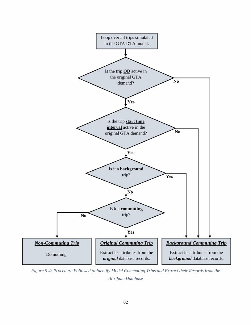
82

Figure 5-4: Procedure Followed to Identify Model Commuting Trips and Extract their Records from the

Attribute Database

No

Yes

Non-Commuting Trip

Do nothing.

Original Commuting Trip

Extract its attributes from the

original database records.

Background Commuting Trip

Extract its attributes from the

background database records.

No

Yes

Yes

Loop over all trips simulated

in the GTA DTA model.

Is the trip OD active in

the original GTA

demand?

Is the trip start time

interval active in the

original GTA demand?

Is it a background

trip?

Is it a commuting

trip?

Yes

No

No

83

After applying the procedure described in the flowchart to all simulated trips in the GTA model,

the detailed information of the identified commuting trips (ID, OD, start time, etc.) along with

their extracted personal and socio-economic attributes are written to files provided as input to the

departure time choice module.

5.5.2. Network-Related Attributes

The second type of data required by the departure time choice model is related to network

average travel times, distances, and costs corresponding to commuters’ ODs at all departure time

intervals. Unlike driver-related attributes, this type of data changes – and is hence recalculated –

following each traffic assignment simulation model run, as illustrated in the system flowchart in

Figure 3-2.

The preparation process of this data type involves processing the detailed path and time

trajectories of around 2 million vehicles, stored in large output files of the simulation model. The

records processed for each vehicle contain its OD, start time, travel time, links traversed, and

time spent on each link along the trip. The travel distance of each commuting trip is calculated

by summing the lengths of links traversed during that trip. Additionally, the tolled links traversed

during the trip are identified to be used by the departure time choice model for toll cost

calculations, as will be described in Section 5.6.

As highlighted earlier, the departure time intervals during which trips are started among certain

OD pairs, are referred to as the active intervals of that OD pair. For each OD pair having

commuting trips in the simulation model, the average travel time and travel distance of that OD

pair at each active interval are calculated by averaging the travel times and distances,

respectively, of trips started during that interval. The travel cost is calculated, by multiplying the

travel distance by the average cost of auto use per unit distance. The value used for the latter

parameter is 0.1534 $/km, as was calculated in Miller et al. (2015) based on average gas and

other car-related operational and maintenance costs in the GTA.

It is important however to mention that the departure time choice model requires the network-

related attributes of each commuter’s OD at all (active and non-active) departure time intervals.

For that purpose, the average travel time, distance, and cost of each non-active interval of certain

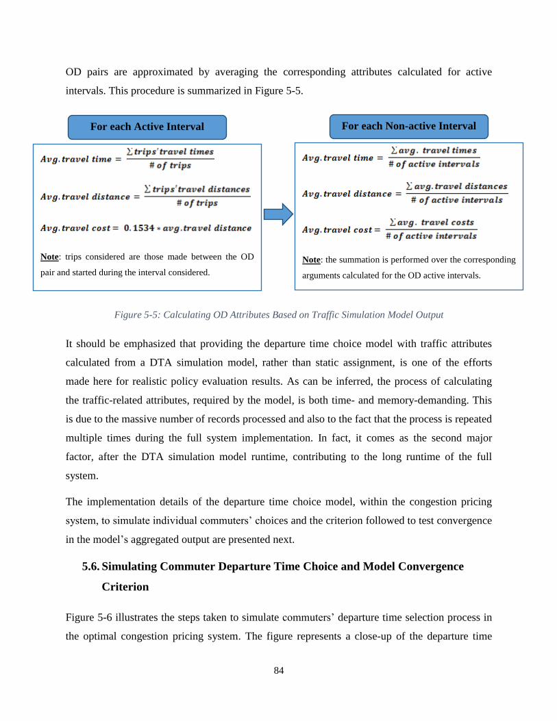
84

OD pairs are approximated by averaging the corresponding attributes calculated for active

intervals. This procedure is summarized in Figure 5-5.

Figure 5-5: Calculating OD Attributes Based on Traffic Simulation Model Output

It should be emphasized that providing the departure time choice model with traffic attributes

calculated from a DTA simulation model, rather than static assignment, is one of the efforts

made here for realistic policy evaluation results. As can be inferred, the process of calculating

the traffic-related attributes, required by the model, is both time- and memory-demanding. This

is due to the massive number of records processed and also to the fact that the process is repeated

multiple times during the full system implementation. In fact, it comes as the second major

factor, after the DTA simulation model runtime, contributing to the long runtime of the full

system.

The implementation details of the departure time choice model, within the congestion pricing

system, to simulate individual commuters’ choices and the criterion followed to test convergence

in the model’s aggregated output are presented next.

5.6. Simulating Commuter Departure Time Choice and Model Convergence

Criterion

Figure 5-6 illustrates the steps taken to simulate commuters’ departure time selection process in

the optimal congestion pricing system. The figure represents a close-up of the departure time

For each Active Interval For each Non-active Interval

Note: trips considered are those made between the OD

pair and started during the interval considered.

Note: the summation is performed over the corresponding

arguments calculated for the OD active intervals.

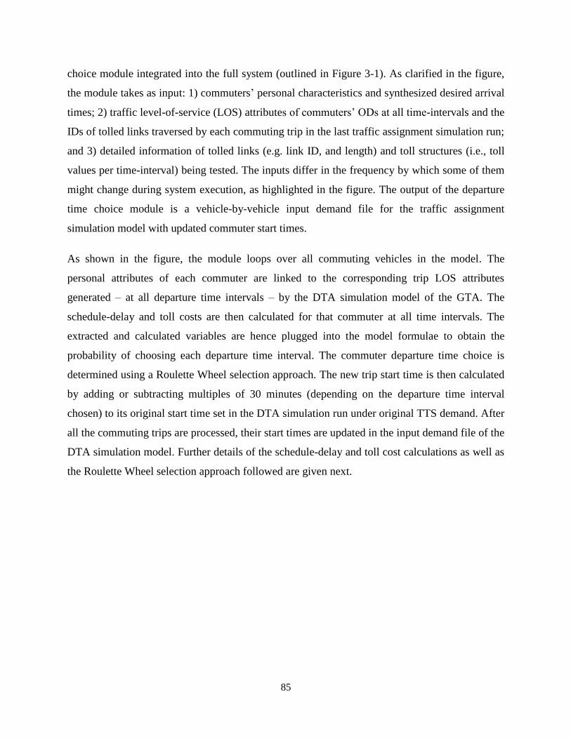
85

choice module integrated into the full system (outlined in Figure 3-1). As clarified in the figure,

the module takes as input: 1) commuters’ personal characteristics and synthesized desired arrival

times; 2) traffic level-of-service (LOS) attributes of commuters’ ODs at all time-intervals and the

IDs of tolled links traversed by each commuting trip in the last traffic assignment simulation run;

and 3) detailed information of tolled links (e.g. link ID, and length) and toll structures (i.e., toll

values per time-interval) being tested. The inputs differ in the frequency by which some of them

might change during system execution, as highlighted in the figure. The output of the departure

time choice module is a vehicle-by-vehicle input demand file for the traffic assignment

simulation model with updated commuter start times.

As shown in the figure, the module loops over all commuting vehicles in the model. The

personal attributes of each commuter are linked to the corresponding trip LOS attributes

generated – at all departure time intervals – by the DTA simulation model of the GTA. The

schedule-delay and toll costs are then calculated for that commuter at all time intervals. The

extracted and calculated variables are hence plugged into the model formulae to obtain the

probability of choosing each departure time interval. The commuter departure time choice is

determined using a Roulette Wheel selection approach. The new trip start time is then calculated

by adding or subtracting multiples of 30 minutes (depending on the departure time interval

chosen) to its original start time set in the DTA simulation run under original TTS demand. After

all the commuting trips are processed, their start times are updated in the input demand file of the

DTA simulation model. Further details of the schedule-delay and toll cost calculations as well as

the Roulette Wheel selection approach followed are given next.

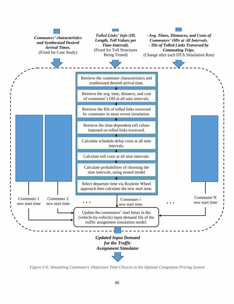
86

Figure 5-6: Simulating Commuters' Departure Time Choices in the Optimal Congestion Pricing System

Retrieve the commuter characteristics and

synthesized desired arrival time.

Retrieve the avg. time, distance, and cost

of commuter’s OD at all nine intervals.

Retrieve the IDs of tolled links traversed

by commuter in most recent simulation.

Calculate schedule-delay costs at all nine

intervals.

Calculate toll costs at all nine intervals.

Calculate probabilities of choosing the

nine intervals, using nested model

formulas.

Retrieve the time-dependent toll values

imposed on tolled links traversed.

Select departure time via Roulette Wheel

approach then calculate the new start time.

Commuter i

new start time

Commuter 2

new start time

Commuter 1

new start time

Commuter N

new start time . . . . . .

Update the commuters’ start times in the

(vehicle-by-vehicle) input demand file of the

traffic assignment simulation model.

Updated Input Demand

for the Traffic

Assignment Simulator

Commuters’ characteristics

and Synthesized Desired

Arrival Times.

(Fixed for Case Study)

- Avg. Times, Distances, and Costs of

Commuters’ ODs at All Intervals.

- IDs of Tolled Links Traversed by

Commuting Trips.

(Change after each DTA Simulation Run)

Tolled Links’ Info (ID,

Length, Toll Values per

Time-Interval).

(Fixed for Toll Structures

Being Tested)

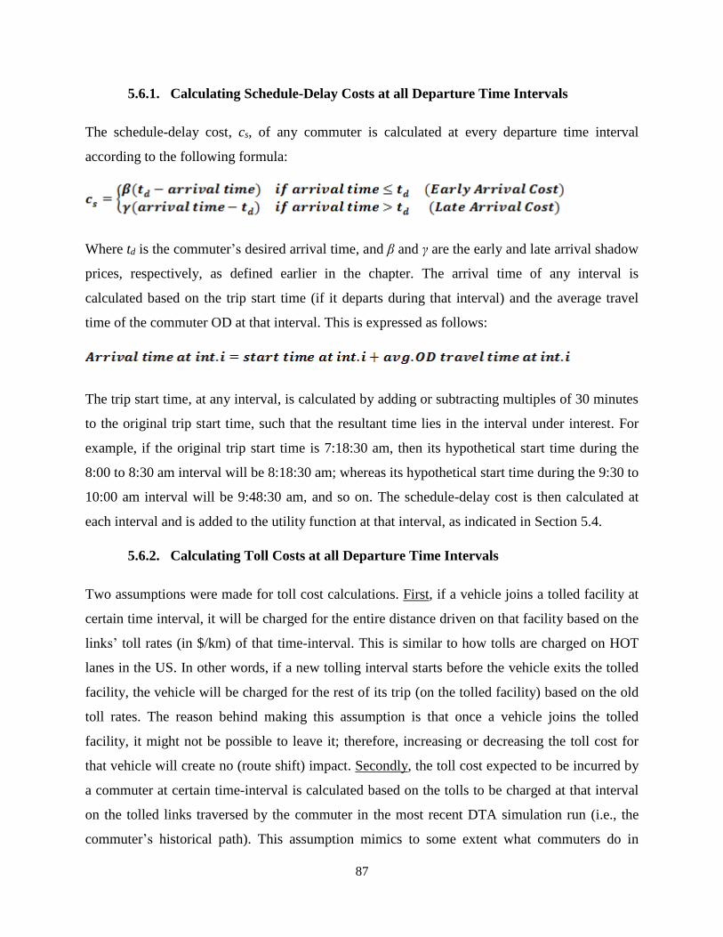
87

5.6.1. Calculating Schedule-Delay Costs at all Departure Time Intervals

The schedule-delay cost, cs, of any commuter is calculated at every departure time interval

according to the following formula:

Where td is the commuter’s desired arrival time, and β and γ are the early and late arrival shadow

prices, respectively, as defined earlier in the chapter. The arrival time of any interval is

calculated based on the trip start time (if it departs during that interval) and the average travel

time of the commuter OD at that interval. This is expressed as follows:

The trip start time, at any interval, is calculated by adding or subtracting multiples of 30 minutes

to the original trip start time, such that the resultant time lies in the interval under interest. For

example, if the original trip start time is 7:18:30 am, then its hypothetical start time during the

8:00 to 8:30 am interval will be 8:18:30 am; whereas its hypothetical start time during the 9:30 to

10:00 am interval will be 9:48:30 am, and so on. The schedule-delay cost is then calculated at

each interval and is added to the utility function at that interval, as indicated in Section 5.4.

5.6.2. Calculating Toll Costs at all Departure Time Intervals

Two assumptions were made for toll cost calculations. First, if a vehicle joins a tolled facility at

certain time interval, it will be charged for the entire distance driven on that facility based on the

links’ toll rates (in $/km) of that time-interval. This is similar to how tolls are charged on HOT

lanes in the US. In other words, if a new tolling interval starts before the vehicle exits the tolled

facility, the vehicle will be charged for the rest of its trip (on the tolled facility) based on the old

toll rates. The reason behind making this assumption is that once a vehicle joins the tolled

facility, it might not be possible to leave it; therefore, increasing or decreasing the toll cost for

that vehicle will create no (route shift) impact. Secondly, the toll cost expected to be incurred by

a commuter at certain time-interval is calculated based on the tolls to be charged at that interval

on the tolled links traversed by the commuter in the most recent DTA simulation run (i.e., the

commuter’s historical path). This assumption mimics to some extent what commuters do in

88

reality to make a departure time choice; they compare travel conditions (time, cost, toll, etc.)

across different times on their historical paths (which might not be the shortest). It should be

mentioned that keeping track of individual vehicle paths is possible through DTA simulation

models, which adds to the benefits of using one of them here.

The toll cost incurred by a vehicle that joins the tolled route during departure time interval i is

hence calculated according to the following formula:

The toll values used in the formula are extracted from the tolled links information entered into

the departure time choice module, as illustrated in Figure 5-6. The toll cost at each interval is

then multiplied by the toll coefficient and added to the travel cost variable of the utility function

corresponding to that interval, as indicated in Section 5.4.

5.6.3. Roulette Wheel Approach for Departure Time Selection

This approach is similar to a Roulette Wheel in a casino. A proportion of the wheel is assigned to

each possible selection based on its weight (i.e., probability of being chosen). A random

selection is then made, similar to how the roulette wheel is rotated. The roulette ball falls in the

bin of an individual choice with a probability proportional to its width. The selection is

implemented by first generating the cumulative probability distribution (CDF) over the list of

choices. A uniform random number is then generated in the range [0, 1] and the inverse of the

CDF of that number determines the choice selected (Back, 1996).

Figure 5-7 shows an example of departure time selection using the Roulette Wheel approach,

based on choice probabilities. Obviously, choices with higher probabilities (i.e., larger portions

of the wheel) have higher chances of being selected; however, the selection made is not

necessarily that having the highest probability, as can be inferred from the figure. It should also

be noted that repeating the Roulette Wheel selection several times (under the same choice

probabilities) might bring different selections, depending on the random numbers generated.

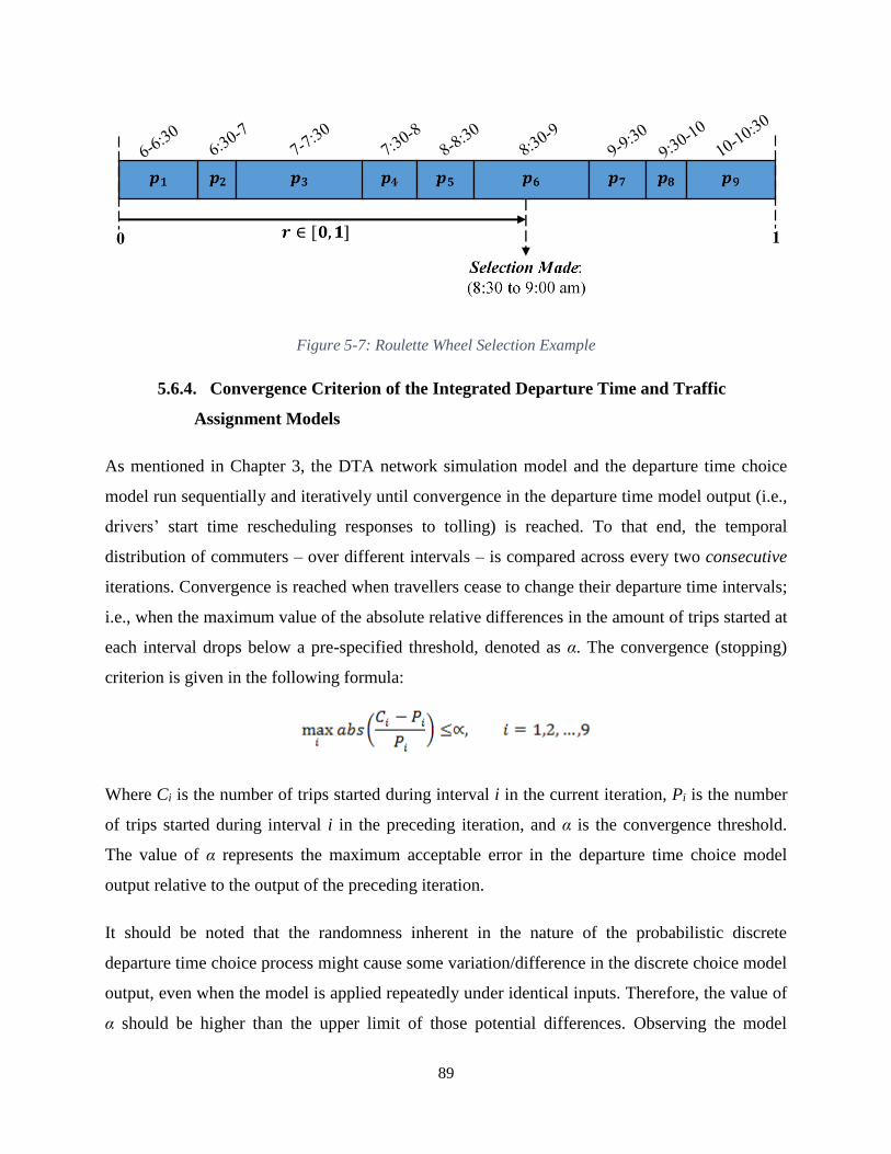
89

Figure 5-7: Roulette Wheel Selection Example

5.6.4. Convergence Criterion of the Integrated Departure Time and Traffic

Assignment Models

As mentioned in Chapter 3, the DTA network simulation model and the departure time choice

model run sequentially and iteratively until convergence in the departure time model output (i.e.,

drivers’ start time rescheduling responses to tolling) is reached. To that end, the temporal

distribution of commuters – over different intervals – is compared across every two consecutive

iterations. Convergence is reached when travellers cease to change their departure time intervals;

i.e., when the maximum value of the absolute relative differences in the amount of trips started at

each interval drops below a pre-specified threshold, denoted as α. The convergence (stopping)

criterion is given in the following formula:

Where Ci is the number of trips started during interval i in the current iteration, Pi is the number

of trips started during interval i in the preceding iteration, and α is the convergence threshold.

The value of α represents the maximum acceptable error in the departure time choice model

output relative to the output of the preceding iteration.

It should be noted that the randomness inherent in the nature of the probabilistic discrete

departure time choice process might cause some variation/difference in the discrete choice model

output, even when the model is applied repeatedly under identical inputs. Therefore, the value of

α should be higher than the upper limit of those potential differences. Observing the model

90

output – across different runs – when applied to the GTA morning commuting trips (around

1,270,000), under identical inputs, it was found that a suitable value for α to be used in this

application is 0.1. The number of iterations required for convergence is generally affected by the

stability of the DTA simulation model output across multiple runs. According to the convergence

criteria specified, it takes the integrated departure time choice and traffic assignment models

around three iterations (of the intermediate loop) to converge in the GTA simulation-based case

studies. This is considered a relatively fast convergence for such a large-scale application.

The number of trips started at any departure time interval is calculated by summing the

probabilities of choosing that interval across all commuters, rather than counting the number of

commuters who selected that interval. This is to avoid the possible bias in departure time

selections due to random number generation and Roulette Wheel selection that might bring

slightly different choices when repeated several times, under identical model inputs. More

specifically, if the random selection process is repeated infinitely large number of times (say n,

where n→∞) for all commuters, the average (over all n trials) number of commuters who

selected each departure time interval (i = 1, 2, … or 9) will be equal to the summation of

probabilities of selecting that interval (pi) among all commuters (Train, 2003). This is expressed

in the following formula:

As highlighted in Chapter 3, the feedback provided to the departure time choice model means

that decisions are not obtained in one step; each individual's choice affects the travel times, costs,

etc. that determine the choices of others. In fact, one-step solutions neglect the interaction

between individuals. Conversely, the feedback component opens the door for such interaction to

affect the final choices. This mimics what happens in reality in response to new policies; people

keep changing their actions and choices, according to the network state and choices of other

travellers, until equilibrium is reached. The final base-case validation results following the

departure time choice model retrofitting and recalibration processes are presented next.

91

5.7. Departure Time Choice Model Validation

In Figure 5-8, the number of commuting trips starting at each half-hour interval and their

corresponding average travel time per km are compared among two simulation runs, whose

measurements are referred to in the figure as “original demand” and “modified demand”. The

total number of commuting trips in the GTA model – for which the departure time choice model

is applied and plots in Figure 5-8 are reported – is around 1,270,000 trips (out of a total of 2

million trips in the model). The measurements under “original demand” are obtained from the

output of a GTA DTA simulation run in base-case conditions (i.e., without tolling) using the

original demand extracted from TTS survey data, without applying the departure time choice

model. On the other hand, those under “modified demand” are obtained from applying the

retrofitted/re-calibrated departure time choice model iteratively with the GTA DTA simulation

model under base-case conditions. As mentioned, the comparison/validation process was

repeated with each set of parameters being calibrated until the best values entailing the minimum

error (between original and modified demand related measurements) were obtained at that

calibration phase, as described in Section 5.4. The patterns shown in Figure 5-8 represent the

best correspondence attained, in the absolute values and the overall trends, between the ‘original’

and ‘modified’ demand-related measurements after performing all model retrofitting/calibration

steps.

92

Figure 5-8: Comparisons between ‘Original’ and ‘Modified’ Demand-related Measurements

The nine departure time intervals used in this model (viz. 6:00-6:30, 6:30-7:00... 10:00-10:30)

were assigned the numerical indices 0, 1... 8. For each vehicle in the simulation model, the

difference between its observed (original) departure time interval index and its estimated one

was calculated at the end of the iterative simulations. The value of the difference lies between -

8–8. Intuitively, the higher the percentage of vehicles with a zero difference (when estimated and

observed departure time intervals coincide) the better. Figure 5-9 shows the percentage of

vehicles whose difference lies in each ‘index difference group’ when applying the calibrated

discrete choice model iteratively with the DTA simulation model in the base-case (i.e., without

tolling). It is shown that the estimated departure time choice of more than 80% of the commuters

lies within three intervals (before or after) from the original (half-hour) choice, which we believe

is reasonable, given the continuous nature of the departure time and the boundary value problems

that may result from time discretization. The findings from Figure 5-8 and Figure 5-9

demonstrate the performance of the calibrated framework when applied to the GTA in the base-

case without tolling.

93

Figure 5-9: Percentage of Commuters vs. Index Difference

5.8. Summary

The discrete choice model has 74 statistically significant parameters, among which only 18

needed to be adjusted for the validation of the model outputs, for the following reasons: 1) to

update the model to be consistent with the 2011 TTS dataset being used, 2) to adapt with the

added schedule-delay and toll cost components, and 3) to compensate for possible bias in output

choices resulting from providing the model with travel times and costs estimated based on the

DTA simulation model, rather than the less accurate static assignment output times and costs

used in the original model estimation. Effort was devoted towards calibrating/retrofitting the

2006 model to the target year of 2011 to meet current research needs. This was carried out for

three reasons: 1) the 2006 model was recently developed; repeating the estimation for 2011 was

beyond the scope of this study; 2) updating a 2006 model using 2011 dataset is a way of using

two repeated cross-sectional data where 2006 data are used for estimation and 2011 data for

validation; and 3) estimating a departure time choice model that captures toll cost and schedule-

delay cost directly was not possible, as neither the 2006 nor the 2011 TTS data contained the

necessary information, i.e. retrofitting was unavoidable. The retrofitting process performed,

however, should not affect the robustness of the original model formulation given its relatively

large number of parameters and statistically significant explanatory variables, as well as the

parameterized root and nested scale parameters.

94

It is important to emphasise that one of the major contributions of this study is the integration of

a behavioural departure time choice model, into the proposed congestion pricing system, to

assess the differential impact of pricing scenarios on drivers’ departure time choices. The model

not only involves travel time, schedule-delay, and toll cost variables, but also considers the

personal and socio-economic attributes of individual drivers. Moreover, it considers users’

heterogeneity in values of (early or late) schedule-delay and desired arrival time.

The estimated measurements plotted in Figure 5-8 and Figure 5-8 are calculated based on the

simulation output obtained from applying the adjusted departure time choice model iteratively

with the DTA simulation model under base-case conditions (i.e., without tolling). This output is

used, throughout this study, in the initial toll calculations and comparative assessment of

different tolling policies. It is hereafter referred to as the “base-case” output, against which toll

policies are evaluated.

The departure time choice model integration process was accompanied by many challenges.

First, the model retrofitting/recalibration process involved several phases and multiple trials

within each phase to attain the parameters achieving the best base-case validation results. The

validation results of each set of parameters tested were obtained through a complete run (taking

multiple hours) of the GTA testbed. In addition, calibrating a single model to describe accurately

the departure time choice behaviour of more than 1.27 million diverse commuting trips in the

GTA was definitely challenging. The ultimate purpose of the model adjustment process was to

guarantee the effectiveness/robustness of the model in estimating the base-case 2011 commuters’

departure time choices; and therefore to trust the model’s ability to forecast commuters’

behavioural responses to future tolling scenarios properly.

Secondly, preparing the driver-related data required by the model entailed time-consuming effort

to process the raw 2011 TTS survey datasets and extract the attributes linked to each (original or

background) commuter identified in the GTA model properly. Thirdly, calculating the network-

related attributes required by the model involved processing records of 2 million vehicles stored

in massive output files, produced by the traffic assignment simulation model. This is undertaken

to 1) calculate the average travel times and costs of commuters’ ODs at every departure time

interval, and 2) identify the tolled links traversed by each commuting vehicle in the model. The

calculation process is obviously time- and computationally demanding. Moreover, it is repeated

95

iteratively – post the termination of each GTA traffic assignment simulation run – to provide the

departure time choice model with the updated network attributes, based on which the model

estimates the new demand profiles to be fed back into the traffic simulation model, and so on

until convergence. As a result, this process represents the second major factor causing the

running time of the full system to be long.

The next chapter presents the first-level of optimal toll determination in the proposed congestion

pricing system, based on the Bottleneck Model. The procedure is discussed and demonstrated

through case studies in the GTA.

96

6. Optimal Congestion Pricing Determination - Level I: Calculating

Time-Dependent Queue-Eliminating Toll Structures Based on the

Bottleneck Model

The optimal toll structures are determined in the congestion pricing system through a bi-level

procedure, as described briefly in Chapter 3. The first level involves the determination of time-

dependent queue-eliminating toll structures for congested facilities. The second level involves

fine-tuning the toll values obtained in the first level to achieve the best network performance,

while considering the large-scale network (route and departure time choice) dynamics in

response to tolling.

This chapter presents the details of the first level, referred to as “Optimal Toll Determination –

Level I” in the optimal congestion pricing system framework outlined in Figure 3-1. The chapter

starts with an overview of the theoretical economic model adopted here for dynamic congestion

pricing, i.e. the Bottleneck Model. After that, the procedure followed to identify the congested

facilities that need to be tolled and to calculate their initial toll structures (based on the

Bottleneck Model) is described. This procedure is then applied and tested on several tolling

scenarios in the GTA. The chapter concludes with a general discussion and insights driven from

the preliminary results of the partially optimized tolling scenarios tested.

6.1. Theoretical Basis: The Bottleneck Model for Dynamic Congestion Pricing

Dynamic models consider that congestion peaks over time then subsides. Therefore, there is a

congestion delay component that peaks with the congestion that the travellers experience.

Dynamic models assume that travellers have a desired arrival time; deviations from which imply

early or late schedule-delays. Travellers who arrive on time during the peak periods encounter

the longest delay; i.e., there is a trade-off between congestion delay and schedule-delay costs.

As mentioned before, the Bottleneck Model involves a single "bottleneck" and assumes that

travellers are homogeneous and have the same desired arrival time, t*. Moreover, the model

assumes that for arrival rates of vehicles not exceeding the bottleneck capacity and in the

absence of a queue, the bottleneck's outflow is equal to its inflow; as a result, no congestion

97

(delay) occurs. When a queue exists, vehicles exit the queue at a constant rate, which is the same

as the bottleneck capacity Vk. Figure 6-1-a illustrates the un-priced equilibrium condition of this

model (i.e., equilibrium in the absence of tolling), and Figure 6-1-b shows the two components

of the total cost c(t) in the un-priced equilibrium condition: travel delay cost cT(t) and schedule-

delay cost cs(t) (early and late arrival costs). The schedule-delay cost is assumed to be a

piecewise linear function in this model. The summation of the two costs (i.e., the total cost) is

constant in the un-priced equilibrium, as illustrated in the figure.

According to Figure 6-1-a, the peak period is considered to start when the inflow exceeds the

bottleneck capacity (i.e., at time tq), resulting in traffic queues and increased travel times that

build up to a maximum when the inflow starts to decrease below capacity (at time tmax). The peak

does not end at this point of time; rather, it ends when all travellers who entered the system –

from the beginning of the peak period – ultimately exit after having queued for a while (i.e., at

time tq’).

The optimal toll in the Bottleneck Model attempts to “flatten” the peak in order to spread the

demand evenly over the same time period. In this case, the price is set such that the inflow equals

road capacity, which in turn equals the outflow. The optimal tolled-equilibrium exhibits the same

pattern of exits from the bottleneck as the un-priced equilibrium, but has a different pattern of

entries. Pricing affects the pattern of entries with a triangular toll schedule, with two linear

segments, which replicate the pattern of travel delay costs in the un-priced equilibrium. This toll

is shown in Figure 6-1-b as τ(t), and results in the same pattern of schedule-delay cost as in the

un-priced equilibrium, but produces zero travel delay cost (i.e. no travel delays exist in the

optimal case). Instead of queueing-delay, travellers trade off the amount of toll to be paid versus

schedule-delay, such that a traveller who arrives right on time t* pays the highest toll, and vice

versa. The resulting tolled-equilibrium queue-entry pattern therefore satisfies an entry rate equal

to the capacity Vk, i.e. the queue entry rate equals the queue exit rate in Figure 6-1-a.

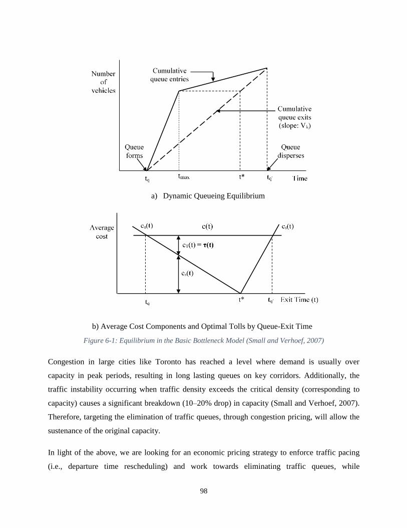
98

a) Dynamic Queueing Equilibrium

b) Average Cost Components and Optimal Tolls by Queue-Exit Time

Figure 6-1: Equilibrium in the Basic Bottleneck Model (Small and Verhoef, 2007)

Congestion in large cities like Toronto has reached a level where demand is usually over

capacity in peak periods, resulting in long lasting queues on key corridors. Additionally, the

traffic instability occurring when traffic density exceeds the critical density (corresponding to

capacity) causes a significant breakdown (10–20% drop) in capacity (Small and Verhoef, 2007).

Therefore, targeting the elimination of traffic queues, through congestion pricing, will allow the

sustenance of the original capacity.

In light of the above, we are looking for an economic pricing strategy to enforce traffic pacing

(i.e., departure time rescheduling) and work towards eliminating traffic queues, while

99

considering drivers’ desired arrival times and the associated schedule-delays. Moreover, the toll

levels should be carefully designed to enforce proper route choices that minimize the total travel

times. In other words, we are seeking congestion pricing policies that achieve the best – spatial

and temporal – traffic distribution and infrastructure utilization to optimize the network

performance (i.e., minimize the total travel times).

Accordingly, the toll structure introduced here is motivated by the theoretical bottleneck pricing

theory, where the key benefits arise from rescheduling (i.e., temporal distribution) of departure

times from the trip origin, resulting in no queueing-delays on tolled facilities. Although the

Bottleneck Model provides the core concept, it is limited to the case of a single bottleneck with

homogeneous travellers having a single desired arrival time. Therefore, the impact of travellers’

heterogeneous attributes and desired arrival times on their departure time choices is not

considered in the model. Additionally, departure time is assumed to be the only choice travellers

have to respond to pricing. A number of studies (van den Berg and Vehoef, 2011; van den Berg,

2014) have analyzed equilibrium in a bottleneck while considering travellers’ heterogeneity in

desired arrival times and/or cost parameters (e.g., VOT and early/late schedule-delay shadow

prices). The optimal time-varying toll obtained in these studies does not have a simple triangular

shape as suggested by the Bottleneck Model; rather, it is increasing and piecewise-convex during

the early intervals, and decreasing and piecewise-convex during the late intervals.

The congestion pricing system proposed here extends the conceptual pricing structure suggested

by the Bottleneck Model – and generalized in subsequent studies while relaxing some of its

unrealistic assumptions by incorporating several desired arrival times and/or cost parameters – to

the more complex and general case of a large urban network with myriad of origin-destination

pairs, trip lengths, travellers’ desired arrival times, routing options, and travel behaviour that

vary across the population. More specifically, the system uses the general pricing rules of the

Bottleneck Model to determine initial toll structures for congested facilities. The procedure

followed for that purpose is described in detail in the next section. Avoiding the unrealistic

assumptions of the Bottleneck Model might bring different impacts of tolling than those obtained

in the tolled-equilibrium output of the model (described earlier). Consequently, the routing and

departure time choice responses to tolling – across the full network (rather than a single

bottleneck) and the entire morning period (rather than the peak period) – are evaluated here

100

through integrated econometric departure time choice and DTA simulation models, described in

detail in previous chapters. The evaluation results of initial toll structures obtained for several

case studies in the GTA are presented in Section 6.3. Based on the evaluation results, initial toll

structures are then adjusted (fine-tuned) through an iterative distributed optimization algorithm

to attain the best network performance, as will be detailed in Chapter 7.

6.2. Initial Toll Structure Design Approach

The optimum toll τ(t) in the Bottleneck Model varies continuously over time, as illustrated in

Figure 6-1-b. It is however impractical to change the toll every second, as suggested by the

model. ‘Step tolls’ are the closest approximation to this ideal situation in practice; different toll

values are set at discrete time intervals, and the toll is constant within each interval, as

highlighted in Figure 3-1.

As reported earlier, the study period is focused on the morning period from 6:00 to 10:30 am

when the majority of commuting trips in the GTA occurs, and hence significant traffic utilizes

the main corridors to Central Business Districts (CBDs) and other employment centres. The

variable-tolling intervals used are the nine half-hour intervals shown in Figure 5-1, for

compatibility with the departure time choice model.

Step tolls might however create negative driving habits when the toll schedule is known by

drivers, depending on the step (time interval) width and the relative toll differences among

adjacent steps. The longer the steps and the larger the toll differences, the more negative the

implications that step tolling might cause in traffic. For example, as the end of a tolling interval

approaches, drivers have an incentive to slow down or to stop before reaching the tolling point,

and wait until the toll is lowered from one interval to the next. This is referred to as the ‘braking

behaviour’ and has been observed in practice in some cities, such as Singapore, Stockholm, and

San Francisco (Lindsey et al., 2012). Braking can intuitively reduce the gains from tolling due to

loss of road effective capacity while drivers are stopped or are slowing down. Drivers might also

speed up in order to pass through the tolling point and avoid a toll increase.

Lindsey et al. (2012) analyzed step-tolling in the Bottleneck Model under the assumption that

drivers stop and wait for a toll to decrease if the cost of waiting (travel time and schedule-delay)

is less than the amount of toll saved. These authors also presented some policy recommendations

101

to prevent or limit braking in designing step-toll systems; e.g., enforcing traffic laws to deter

stopping in the middle of traffic lanes or parking on the shoulder, imposing minimum speed

limits to discourage slowing down, introducing five-minute graduated rates between half-hour

tolling periods, and designing sophisticated systems with distance-based charges instead of

location-based toll collection schemes (to avoid braking problems arising when tolls are levied at

specific locations).

In light of this discussion, some steps were taken to lessen the undesired consequences of step-

tolling. As mentioned earlier, the tolling scheme adopted in the congestion pricing system is

distance-based: each vehicle pays according to the distance travelled on tolled facilities. This

tolling scheme aims to attain spatial equity besides diminishing the incentives for drivers to slow

down or stop before specific toll-collection locations. Additionally, possible inaccuracies in

base-case queueing-delays estimated from DTA simulation might bring large gaps in toll values

of adjacent intervals. Accordingly, the initial step tolls – determined based on the Bottleneck

Model – undergo a toll smoothing procedure to avoid substantial toll changes, as will now be

described in detail.

Figure 6-2 illustrates the procedure followed to determine initial toll structure (i.e., distinct toll

values for the nine half-hour tolling intervals) for each congested facility of interest in the tolling

scenario, based on the Bottleneck Model pricing rules. The figure represents a close-up of the

“Optimal Toll Determination – Level I” module integrated into the optimal congestion pricing

system (outlined in Figure 3-1). The purpose of the procedure is to 1) determine whether or not

each facility of interest needs to be tolled and 2) calculate initial toll structures for facilities that

should be tolled. This procedure is applied once at the beginning of the full system

implementation for a certain case study. As shown in Figure 6-2, the module takes as input the

information of facilities under interest (to be tolled) in the tolling scenario; e.g., corresponding

links, speed limit, and base-case traffic attributes. On the other hand, the output of the module is

the tolled links information including link ID, length, start node, end node, facility number, and

initial time-dependent toll values. The facility number is a unique ID of the tolled facility to

which the link belongs.

As described in Section 6.1, the optimal toll in the Bottleneck Model attempts to flatten the peak

(i.e., spread the demand evenly over the same period) through a triangular toll schedule that

102

replicates the pattern of queueing-delay costs in the un-priced equilibrium. This toll schedule

results in zero queueing-delays in the optimal case, according to the Bottleneck Model findings.

The queueing-delay, as illustrated in Figure 6-1-a, represents the excess travel delay over the

‘travel time at capacity,’ defined as the time taken to cross the road when the inflow rate equals

road capacity, Vk.

6.2.1. Estimating Queueing-Delay Patterns

Following the same queue-eliminating optimal pricing rule adopted in the Bottleneck Model, the

toll structure determination procedure, illustrated in Figure 6-2, starts with estimating the pattern

of queueing-delay for each facility of interest based on the DTA simulation output in the base-

case. Obviously, the purpose of queue-eliminating tolling is to enforce traffic pacing (i.e.,

departure time rescheduling) that works towards eliminating traffic queues (i.e., hyper-

congestion), hence achieving the optimum infrastructure utilization level of tolled facilities.

Accordingly, if the estimated base-case travel times of certain facility are below or close to the

facility ‘travel time at capacity’ at all times (i.e., if the queueing-delay is zero or negligible at all

times), then the facility should not be tolled. Tolling such facility will unnecessarily cut its

demand level and hence underutilize its available capacity, which is against the benefits of

tolling targeted here.

The queueing-delay, at a certain time t, is defined as the average extra travel time incurred by

vehicles entering the facility at t over the facility travel time at capacity (i.e., the travel time

when the inflow equals the road capacity). The queueing-delay, therefore, represents the extra

travel time incurred due to ‘hyper-congestion’, as indicated in the following formula:

The travel time at capacity is calculated by dividing the facility length by the speed value at

capacity. This value is determined from the speed corresponding to the maximum flow in the

traffic flow model used in the DTA simulation model. For instance, according to the traffic flow

model parameters used (reported in Section 4.3.2), the critical density and speed values

associated with the maximum flow on a freeway having a 100 km/hr speed limit are 29 veh/km

and 57 km/hr, respectively, as illustrated in Figure 6-3. Therefore, the travel time at capacity for

an 18 km-long facility (like the Gardiner Expressway) is calculated as 19 minutes according to

103

this procedure. It should be emphasized that the queue-eliminating tolling adopted here,

following the Bottleneck Model general pricing rules, addresses hyper-congestion only to restore

operation to the capacity point, leading to full utilization of the network. In other words, no toll is

imposed so long as the ‘base-case travel time’ is below the ‘travel time at capacity’, even if the

former is higher than the ‘free-flow travel time’. It should also be noted that although the traffic

flow models used in the DTA simulation software feature hyper-congestion (i.e. decreased flow

values as density exceeds the critical density), they do not incorporate the capacity drop at the

critical density (as can be observed in Figure 6-3). Therefore, the anticipated benefits from the

‘restored capacity’, due to hyper-congestion elimination, cannot be explicitly measured under

those models.

Unlike the assumption of a bottleneck having a single entrance and exit, facilities considered to

be tolled in reality have multiple entrances (on-ramps) and exits (off-ramps). Therefore, it

becomes challenging to estimate the (time-dependent) travel time on a facility accurately, given

that vehicles might join and leave it at different intermediate locations. That is, the time

experienced by each vehicle on the facility does not generally represent the travel time required

to cross the entire facility. Accordingly, the base-case travel time pattern of each facility is

approximated here by summing the travel times of the individual facility links. More

specifically, the average travel time required to cross the facility by vehicles entering during

certain time-interval, T, is calculated by summing links’ average travel times during that interval.

The link average travel time during T is calculated by dividing the link length by the average link

speed during T. Minute-by-minute link-related statistics, reported in the output of the DTA

simulation model, are processed to calculate the required average link speeds and hence travel

times. The procedure followed to calculate the facility average travel time at any interval T is

summarized as:

The selection of T involves a tradeoff between choosing a small interval to avoid diluting traffic

dynamics from one side, and choosing a large interval to account for the time taken to cross the

entire facility from another side (since link times are summed over the same interval). A 15 min

value was chosen for T based on the range of lengths, hence travel times, of facilities selected to

104

be tolled through different scenarios considered in this study. Larger values tested for T resulted

in the inaccurate estimation of peak start and end times, hence counterproductive impacts of

some toll structures calculated based on those values. For each facility, the queueing-delay is

calculated by subtracting the corresponding travel time at capacity from the estimated travel time

pattern, when the latter exceeds the former; otherwise, the queueing-delay is zero.

6.2.2. Initial Toll Structure Determination

The beginning and end times of the estimated queueing-delay pattern of each facility define the

peak period start and end times of that facility, respectively. According to the Bottleneck Model,

a continuous triangular toll pattern that replicates the queueing-delay pattern – i.e., increases

from zero up to a maximum value, then falls back to zero when the queues are clear – should be

imposed on the facility during that period. This is however approximated here through step tolls

in which distinct toll values are imposed on half-hour tolling intervals, as mentioned earlier. The

first and last tolling intervals of each facility are identified as the half-hour intervals during

which the peak period of that facility starts and ends, respectively.

As mentioned, the toll pattern of each congested facility should replicate its base-case estimated

queueing-delay pattern in order to attain the desired rescheduling benefits of variable tolling.

Therefore, the toll is assigned a zero value during early and late intervals having zero queueing-

delay, whereas it is assigned the maximum value during the interval having the largest average

queueing-delay. Similarly, toll levels (indicated by the maximum toll values) corresponding to

different congested facilities should be proportional to their congestion levels in order to obtain

the desired route shift impacts of tolling. The estimated ‘maximum queueing-delay per km’

values of different congested facilities (having distinct lengths) indicate their congestion levels.

In other words, route shifts should be taken into account in addition to temporal shifts.

As a reference, a toll value of 0.15 $/km should be set per interval for every 1 min/km average

‘queueing-delay per km’ experienced in the base-case during that interval. This value was found

– among multiple values tested – to create moderate route shifts resulting in an adequate capacity

utilization level, under the average VOT used in the simulation model. Accordingly, the toll

value at each tolling interval (i = 1, 2… 9) for every congested facility is calculated by

105

multiplying 0.15 by the average ‘queueing-delay per km’ estimated on the facility during that

interval.

Some factors might occasionally cause abrupt changes in toll values calculated for adjacent time-

intervals. Possible inaccuracies in travel time (hence queueing-delay) estimation are among those

factors. Additionally, averaging traffic attributes (e.g. travel time) over discrete time-intervals

might dilute rapid traffic changes happening during some intervals. Therefore, the calculated toll

structures undergo a smoothing procedure to avoid the negative consequences of large toll gaps,

outlined earlier. The procedure involves slightly increasing or decreasing some toll values and/or

extending the tolling period, while preserving the general structure of the tolls. The procedure

aims to obtain a smoother toll structure, as illustrated through an example provided in Figure 6-4.

The toll structure calculated for each facility is applied simultaneously on all links belonging to

that facility. In other words, a unique toll value (in $/km) is imposed on all links belonging to the

same facility at each time interval. This unique value changes (over all links) from one interval

to another, depending on the toll structure. However, non-equal toll values are generally imposed

on links belonging to different tolled facilities at any given interval.

The initial toll structure design procedure, described in this section and summarized in Figure

6-2, resembles the first step towards optimal congestion pricing determination. It answers the

questions of what, when, and how much to be tolled. The procedure is applied and tested through

several tolling scenarios in the GTA presented in the following section. It should be emphasized

that this procedure is general in the sense that it can determine the queue-eliminating toll

structure replicating any congestion pattern over time, whether having a single or multiple peaks

(within the analysis period).

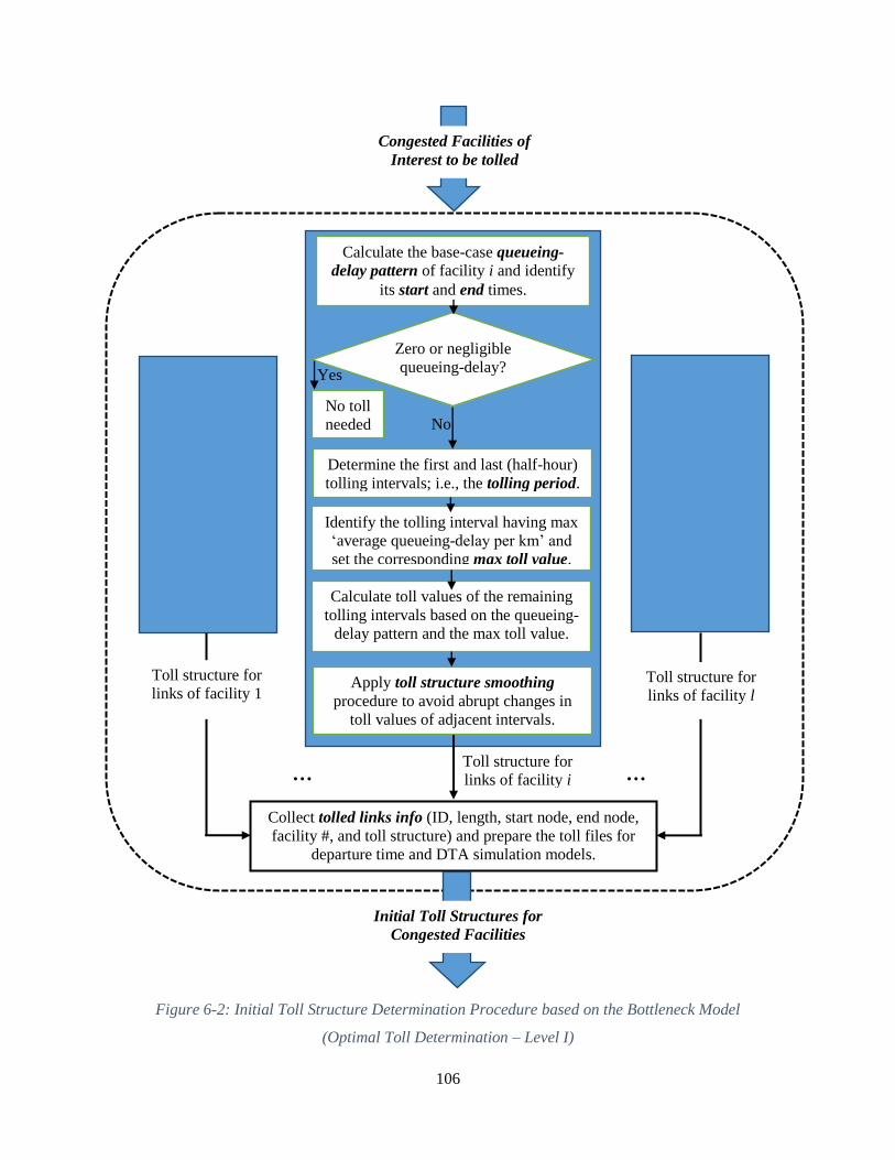
106

Figure 6-2: Initial Toll Structure Determination Procedure based on the Bottleneck Model

(Optimal Toll Determination – Level I)

Collect tolled links info (ID, length, start node, end node,

facility #, and toll structure) and prepare the toll files for

departure time and DTA simulation models.

Calculate the base-case queueing-

delay pattern of facility i and identify

its start and end times.

Identify the tolling interval having max

‘average queueing-delay per km’ and

set the corresponding max toll value.

Zero or negligible

queueing-delay?

Calculate toll values of the remaining

tolling intervals based on the queueing-

delay pattern and the max toll value.

Apply toll structure smoothing

procedure to avoid abrupt changes in

toll values of adjacent intervals.

No toll

needed

.

Determine the first and last (half-hour)

tolling intervals; i.e., the tolling period.

Yes

No

Toll structure for

links of facility i

Toll structure for

links of facility 1

Toll structure for

links of facility l

… …

Congested Facilities of

Interest to be tolled

Initial Toll Structures for

Congested Facilities

107

Figure 6-3: Traffic Density and Speed at Capacity

Figure 6-4: Toll Structure Smoothing - Illustrative Example

6.3. Application and Evaluation of the Initial (Sub-Optimal) Toll Design

Approach through Tolling Scenarios in the GTA

The implemented congestion pricing system is intended to test different tolling scenarios; e.g.

single or multiple freeways, urban corridors, HOT lanes, a sub-network and cordon tolls. In this

study, the system is applied to two test scenarios of tolling major freeways in the GTA while

capturing the regional effects across the entire region. The route selected to be tolled in the first

scenario is the Gardiner Expressway (GE), which is considered as the main artery running

through Downtown Toronto. In the second scenario, tolled facilities are extended to include the

Don Valley Parkway (DVP) and the express lanes of Highway 401, in addition to the GE.

108

For each tolling scenario, the initial (sub-optimal) toll structures of the facilities under interest

are first determined, using the approach described in Section 6.2. The calculated toll structures

are then tested through the integrated testbed of departure time and GTA DTA simulation

models. More specifically, the output of the “Optimal Toll Determination – Level I” module (in

Figure 3-1) is directly entered to the testbed; i.e., the optimization algorithm module is not

activated at this stage. The system terminates when the second level of equilibrium (i.e., the

departure time choice convergence) is reached under the tolling scenario tested.

The simulation modelling platform generates output statistics at different levels: network-wide,

link-based, and trip-based, as described in Chapter 4. The statistics produced vary in volume and

frequency of generation. The initial toll structures of each scenario are evaluated by processing

the simulation output data and calculating appropriate network performance measures at various

levels (i.e. network, tolled facilities, and affected travellers), as will be illustrated through the

tolling scenarios presented next.

6.3.1. Scenario I - Tolling the Gardiner Expressway

The purpose of this scenario is to study the effectiveness of the system proposed in the

evaluation of variable (as opposed to flat) congestion-pricing policies. To that end, two tolling

structures are investigated: 1) variable tolling structure estimated based on the Bottleneck Model

pricing rules (described above), and 2) flat tolling across all time-intervals. A single route is

selected to be tolled in this scenario; equal toll values are imposed on both route directions at any

time interval, as a first implementation. The route selected to be tolled is the Gardiner

Expressway (GE). The GE, as shown in Figure 4-1, is the main artery running through

Downtown Toronto, the core and economic hub of the GTA and arguably Canada. The

expressway is 18 km long between Highway 427 and the Don Valley Parkway (DVP). It is 6–10

lanes wide in varying locations. The number of commuting trips during the 6:00 to 10:30 am

morning period in a typical weekday on the GE corridor (i.e., the Gardiner Expressway and its

parallel arterials on both directions) is approximately 90,000.

In addition to the fact that the GE suffers from extended periods of congestion, there is an

ongoing debate on whether to tear it down, to toll it and use the revenue for its maintenance, or

to apply other hybrid proposals to improve its operation. Hence, the GE was the first choice to

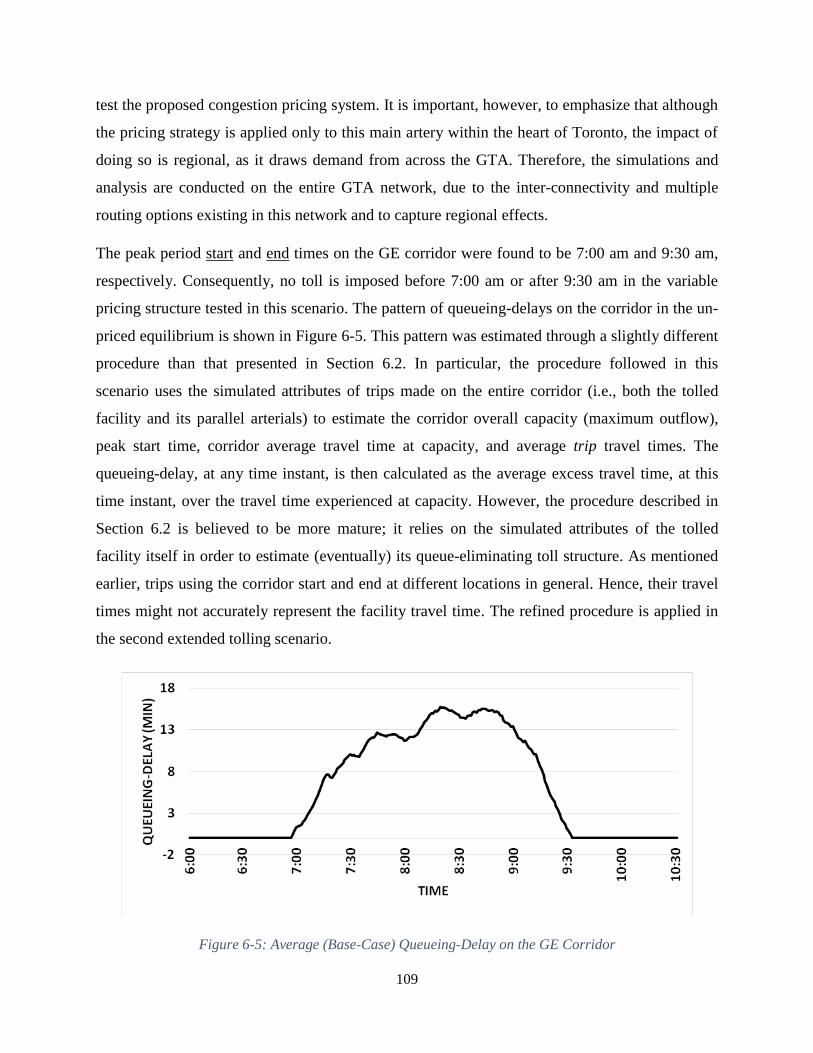
109

test the proposed congestion pricing system. It is important, however, to emphasize that although

the pricing strategy is applied only to this main artery within the heart of Toronto, the impact of

doing so is regional, as it draws demand from across the GTA. Therefore, the simulations and

analysis are conducted on the entire GTA network, due to the inter-connectivity and multiple

routing options existing in this network and to capture regional effects.

The peak period start and end times on the GE corridor were found to be 7:00 am and 9:30 am,

respectively. Consequently, no toll is imposed before 7:00 am or after 9:30 am in the variable

pricing structure tested in this scenario. The pattern of queueing-delays on the corridor in the un-

priced equilibrium is shown in Figure 6-5. This pattern was estimated through a slightly different

procedure than that presented in Section 6.2. In particular, the procedure followed in this

scenario uses the simulated attributes of trips made on the entire corridor (i.e., both the tolled

facility and its parallel arterials) to estimate the corridor overall capacity (maximum outflow),

peak start time, corridor average travel time at capacity, and average trip travel times. The

queueing-delay, at any time instant, is then calculated as the average excess travel time, at this

time instant, over the travel time experienced at capacity. However, the procedure described in

Section 6.2 is believed to be more mature; it relies on the simulated attributes of the tolled

facility itself in order to estimate (eventually) its queue-eliminating toll structure. As mentioned

earlier, trips using the corridor start and end at different locations in general. Hence, their travel

times might not accurately represent the facility travel time. The refined procedure is applied in

the second extended tolling scenario.

Figure 6-5: Average (Base-Case) Queueing-Delay on the GE Corridor

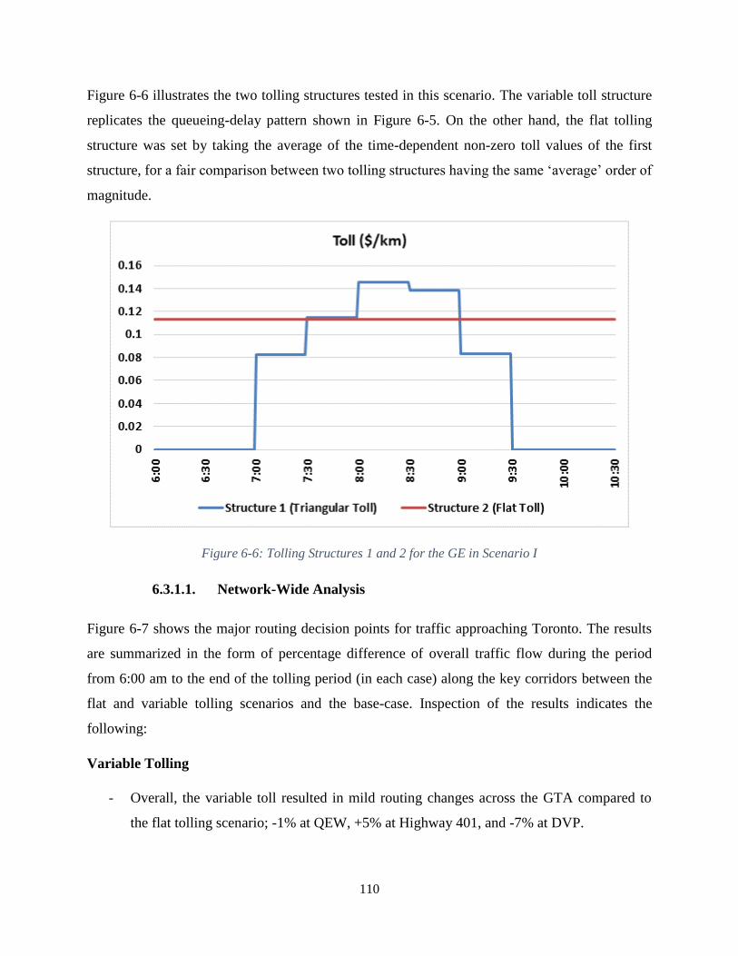
110

Figure 6-6 illustrates the two tolling structures tested in this scenario. The variable toll structure

replicates the queueing-delay pattern shown in Figure 6-5. On the other hand, the flat tolling

structure was set by taking the average of the time-dependent non-zero toll values of the first

structure, for a fair comparison between two tolling structures having the same ‘average’ order of

magnitude.

Figure 6-6: Tolling Structures 1 and 2 for the GE in Scenario I

6.3.1.1. Network-Wide Analysis

Figure 6-7 shows the major routing decision points for traffic approaching Toronto. The results

are summarized in the form of percentage difference of overall traffic flow during the period

from 6:00 am to the end of the tolling period (in each case) along the key corridors between the

flat and variable tolling scenarios and the base-case. Inspection of the results indicates the

following:

Variable Tolling

- Overall, the variable toll resulted in mild routing changes across the GTA compared to

the flat tolling scenario; -1% at QEW, +5% at Highway 401, and -7% at DVP.

111

- At the GE, only 5% divergence was observed at the bifurcation to Lake Shore, resulting

in maximizing the efficiency of the downstream sections of the GE.

Flat Tolling

- Overall, the flat toll resulted in more pronounced re-routing patterns across the GTA

compared to variable tolling; showing -2% at QEW, +5% at Highway 401, and -8% at

DVP. Flat tolling is less conducive to departure time changes, as all periods have the

same toll; therefore, its impact is predominantly on re-routing.

- On the GE, significant divergence (re-routing) was observed at the bifurcation to Lake

Shore, resulting in shockwave and congestion upstream of this bifurcation. This

congestion resulted in – interestingly – less flow on the GE downstream the off-ramp to

Lake Shore, i.e., underutilizing the GE by as much as 44%. This observation was

confirmed by the low speed values (20–28 km/hr.) along the sections of the GE upstream

of the off-ramp.

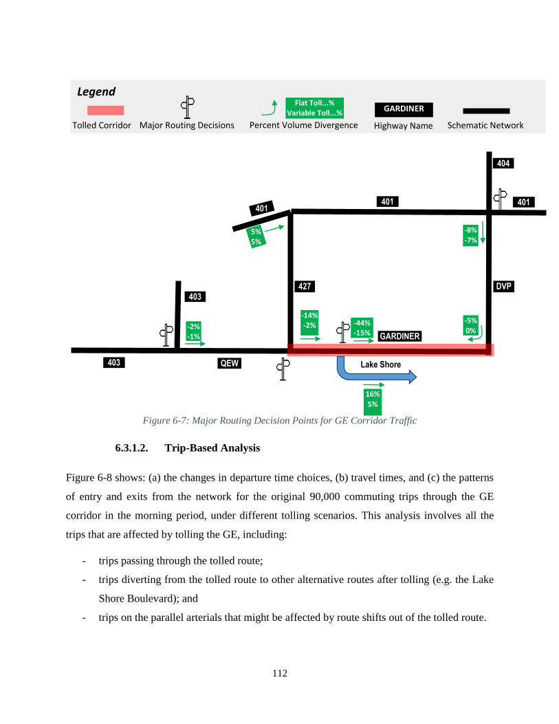
112

Figure 6-7: Major Routing Decision Points for GE Corridor Traffic

6.3.1.2. Trip-Based Analysis

Figure 6-8 shows: (a) the changes in departure time choices, (b) travel times, and (c) the patterns

of entry and exits from the network for the original 90,000 commuting trips through the GE

corridor in the morning period, under different tolling scenarios. This analysis involves all the

trips that are affected by tolling the GE, including:

- trips passing through the tolled route;

- trips diverting from the tolled route to other alternative routes after tolling (e.g. the Lake

Shore Boulevard); and

- trips on the parallel arterials that might be affected by route shifts out of the tolled route.

Legend

GARDINER Flat Toll...%

Variable Toll...%

403 QEW

GARDINER

401

DVP

404

403 427

-2% -1%

5% 5%

401 401

16% 5%

-5% 0%

-8% -7%

-44% -15%

-14% -2%

Lake Shore

Tolled Corridor Major Routing Decisions Percent Volume Divergence Highway Name Schematic Network

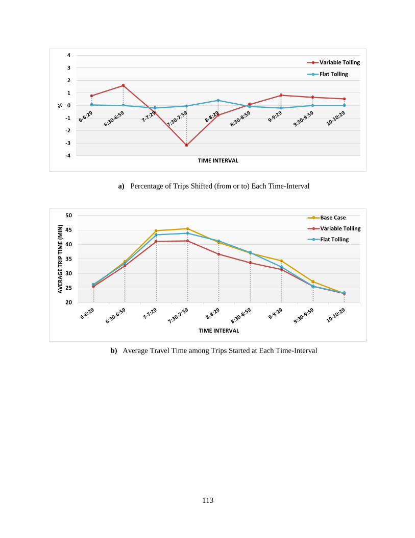
113

-4

-3

-2

-1

0

1

2

3

4%

TIME INTERVAL

Variable Tolling

Flat Tolling

a) Percentage of Trips Shifted (from or to) Each Time-Interval

20

25

30

35

40

45

50

AV

ERA

GE

TRIP

TIM

E (M

IN)

TIME INTERVAL

Base Case

Variable Tolling

Flat Tolling

b) Average Travel Time among Trips Started at Each Time-Interval

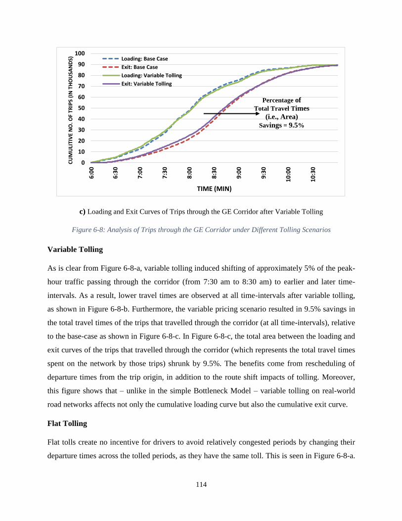
114

c) Loading and Exit Curves of Trips through the GE Corridor after Variable Tolling

Figure 6-8: Analysis of Trips through the GE Corridor under Different Tolling Scenarios

Variable Tolling

As is clear from Figure 6-8-a, variable tolling induced shifting of approximately 5% of the peak-

hour traffic passing through the corridor (from 7:30 am to 8:30 am) to earlier and later time-

intervals. As a result, lower travel times are observed at all time-intervals after variable tolling,

as shown in Figure 6-8-b. Furthermore, the variable pricing scenario resulted in 9.5% savings in

the total travel times of the trips that travelled through the corridor (at all time-intervals), relative

to the base-case as shown in Figure 6-8-c. In Figure 6-8-c, the total area between the loading and

exit curves of the trips that travelled through the corridor (which represents the total travel times

spent on the network by those trips) shrunk by 9.5%. The benefits come from rescheduling of

departure times from the trip origin, in addition to the route shift impacts of tolling. Moreover,

this figure shows that – unlike in the simple Bottleneck Model – variable tolling on real-world

road networks affects not only the cumulative loading curve but also the cumulative exit curve.

Flat Tolling

Flat tolls create no incentive for drivers to avoid relatively congested periods by changing their

departure times across the tolled periods, as they have the same toll. This is seen in Figure 6-8-a.

0

10

20

30

40

50

60

70

80

90

100

6:0

0

6:3

0

7:0

0

7:3

0

8:0

0

8:3

0

9:0

0

9:3

0

10

:00

10

:30

CU

MU

LITI

VE

NO

. OF

TRIP

S (I

N T

HO

USA

ND

S)

TIME (MIN)

Loading: Base Case

Exit: Base Case

Loading: Variable Tolling

Exit: Variable Tolling

Percentage of

Total Travel Times

(i.e., Area)

Savings = 9.5%

115

This scenario outperforms the base-case by only 2% net savings in the total travel times

compared to 9.5% in the variable tolling case. The benefits under flat tolling come solely from

the route shift impacts of tolling. However, as is clear in Figure 6-8-b, this gain is realized more

at early and late intervals, while some deterioration in travel times is observed at peak time-

intervals (i.e. 8–9 am). Further explanation for these findings will be given in the next section.

6.3.1.3. Tolled Route-Based Analysis

Figure 6-9 shows the average travel times on the tolled route (the GE), eastbound direction, from

Highway 427 to the DVP. The times are reported at each time interval for different tolling

scenarios.

0

5

10

15

20

25

30

35

Gar

din

er T

rave

l Tim

e (m

in)

Time Interval

Base Case

Variable Tolling

Flat Tolling

Figure 6-9: Average Travel Time on the Gardiner Expressway Eastbound (from 427 to DVP)

Variable Tolling

As seen in Figure 6-9, variable tolling entails a noticeable decrease in travel times on the tolled

route; especially at the middle congested time-intervals. The maximum observed saving is 7 min

(out of 27 min), i.e. around 25 %, at the 8:00 to 8:30 am time-interval.

Flat Tolling

Flat tolling results in improvements in travel times at early and late intervals. However, it causes

a significant increase in travel times on the tolled route from 8:30 to 9:30 am, as clearly shown in

Figure 6-9, which agrees with the findings from the trip-based analysis. The deterioration occurs

116

due to the excessive demand at peak hours that did not shift to other time-intervals due to the

absence of incentives (i.e., no toll variation over time). This demand tries to exit the tolled route

(the GE) to the immediate parallel arterials (Lake Shore Boulevard), and is limited by off-ramp

and arterial capacity constraints. Therefore, it creates a shockwave/congestion upstream that

blocks the off-ramp and backs up onto the tolled route itself at peak hours, which is very

counterproductive. In fact, this observation demonstrates how flat tolling on real-world road

networks (in which congestion propagates in the form of spillbacks, shockwaves, etc.) can have

appreciably different effects than those suggested by studies of single links or toy networks.

6.3.1.4. Discussion and Conclusions

It can be concluded from the analysis of different tolling structures presented in this scenario (on

network, trip, and tolled-route bases) that:

1. In a large-scale interconnected network (like the GTA) where long-distance trips have

diverse routing options, tolling a relatively short, yet major, highway like the GE creates

temporal and spatial traffic changes network-wide that go beyond the tolling interval and

the tolled route. This confirms the importance of conducting the simulations on a regional

scale for policy determination and assessment.

2. More benefits are gained from departure time re-scheduling due to variable pricing,

compared to just re-routing as in flat tolling. This emphasizes the importance of the

integrated departure time module to the proposed variable congestion pricing framework,

to provide realistic modelling of users' individual departure time responses to variable

pricing policies.

3. Pricing that only induces re-routing (and no departure time re-scheduling), or excessive

re-routing due to, for instance, overpricing, can send traffic to off-ramps to parallel routes

so aggressively that it blocks the off-ramp and backs up onto the main freeway, limiting

access to the priced road itself, which is not only counterproductive but also nullifies the

very purpose of pricing itself. This emphasizes the importance of variable pricing to

mirror congestion patterns over time, which is the methodological basis (adapted from

the Bottleneck Model) of the proposed variable tolling framework.

117

6.3.2. Scenario II - Tolling the Gardiner Expressway, the Don Valley Parkway, and

401 Express Lanes

The purpose of the first experiment was to test the system’s functionality and effectiveness

through a scenario involving a single, yet vital, tolled route with equal toll structures on both

directions. The facilities to be tolled are extended in this scenario include the DVP and the

express lanes of Highway 401, in addition to the GE, as highlighted in Figure 6-10. The 401

Express is divided into three segments in the analysis, separated by major north-south highways,

as is clear in the figure. Moreover, the toll structures are differentiated along opposite directions

of each facility/segment, resulting in a total of 10 separate routes to be considered for tolling, as

illustrated in the figure. A single (sub-optimal) toll structure is determined and imposed on each

route.

Figure 6-10: Routes to be tolled in Scenario II (Google Maps)

The DVP is a 15 km-long expressway connecting the GE in Downtown Toronto with Highway

401. It has six lanes for most of its length and eight lanes north of York Mills Rd. The DVP is

the only north-south expressway serving Toronto’s Downtown. Consequently, it suffers from

significant traffic congestion during the morning and afternoon/evening periods, and is

GE

GE-EB

GE-WB

DV

P

DV

P-

NB

DV

P-

SB

401-Segment 2

401-EB-2

401-WB-2

401-Segment 1

401-EB-1

401-WB-1

401-Segment 3

401-EB-3

401-WB-3

Route

to be

tolled

118

considered – along with the GE – as among Toronto’s busiest municipal routes. There is

increased municipal interest to examine various tolling options on the GE and the DVP for the

primary purpose of offsetting their capital, operating, and maintenance costs (Lively and Rossini,

2015). Accordingly, they have been selected among the facilities to be tolled in this scenario.

However, the primary purpose of tolling in this study is not to raise funds for municipalities, but

rather to alleviate traffic congestion on tolled routes through variable tolling, while considering

network-wide performance.

Highway 401 is an 828 km-long 400-series highway in the Canadian province of Ontario. It

extends from Windsor in the west to the Ontario-Quebec border in the east. The section of

Highway 401 passing through Toronto is one of the busiest highways in the world (Allen, 2011).

The entire route is maintained by the Ministry of Transportation Ontario (MTO).

The highway expands into a collector-express system as it approaches Hurontario Street in

Mississauga. The system divides each direction into collector and express lanes, creating four

carriageways along the highway. Collector lanes are connected to every interchange, through on-

and off-ramps. Express lanes, on the other hand, are only connected to few interchanges. Access

between collector and express lanes is available at several transfer points. The purpose of the

collector-express system is to improve traffic flow for both local and long-distance trips.

The collector-express system stretches for more than 55 km along the highway, including a 5 km

gap east of Highway 427 all the way to Kipling Ave (noticed between segments 1 and 2 in

Figure 6-10). Only express lanes are selected to be tolled in this scenario, leaving collector lanes

as a free alternative. The express lanes are divided into three segments in the analysis as follows:

Segment 1: extends from Hurontario Street in the west to Highway 427 in the east.

Segment 2: extends from Kipling Ave in the west to DVP in the east.

Segment 3: extends from DVP in the west to Pickering in the east.

As mentioned, the tolling structures are differentiated among both eastbound (EB) and

westbound (WB), or northbound (NB) and southbound (SB), directions of each facility/segment

selected to be tolled. The number of commuting trips (to which the departure time choice model

is applied) passing through the routes to be tolled and their parallel arterials during the 6:00 to

119

10:30 am morning period is around 455,000 trips, which represents around 25% of the total

demand.

The initial (sub-optimal) toll structures estimated for the 10 routes selected to be tolled in this

scenario are illustrated in

Table 6-1. These structures were obtained using the ‘Optimal Toll Determination – Level I’

module outlined in Figure 6-2 and described in detail in Section 6.2. According to the criterion

followed, it was concluded that no tolling was needed for the westbound express lanes of 401-

segment 1 (401-WB-1), nor for the eastbound express lanes of 401-segment 3 (401-EB-3) in the

morning peak. It can also be seen from Table 6-1 that the toll structures estimated for different

routes, even those corresponding to opposite directions of the same facility/segment, vary in their

start and end times as well as overall toll levels. This is due to the fact that those routes have

different congestion levels and queueing-delay patterns in the base-case. For example, the

southbound lanes of the DVP are usually more congested in the morning peak than northbound

lanes due to the extra traffic heading to Downtown Toronto during that period, and vice versa.

Comparing the initial toll structures of GE-EB and GE-WB with the variable tolling structure

estimated in the first scenario for the GE (Figure 6-6), it can be observed that the highest toll

value in the latter (0.15 $/km) is close to the average of the highest toll values estimated

individually for both directions in the current scenario (i.e. 0.11 $/km and 0.22 $/km). This

agrees with the fact that the variable tolling structure in the first scenario was estimated based on

the average queueing-delay pattern of all GE corridor users in both directions, as described

before.

Table 6-1: Initial (Sub-Optimal) Toll Structures Derived for Scenario II

Route Toll Structure ($/km)

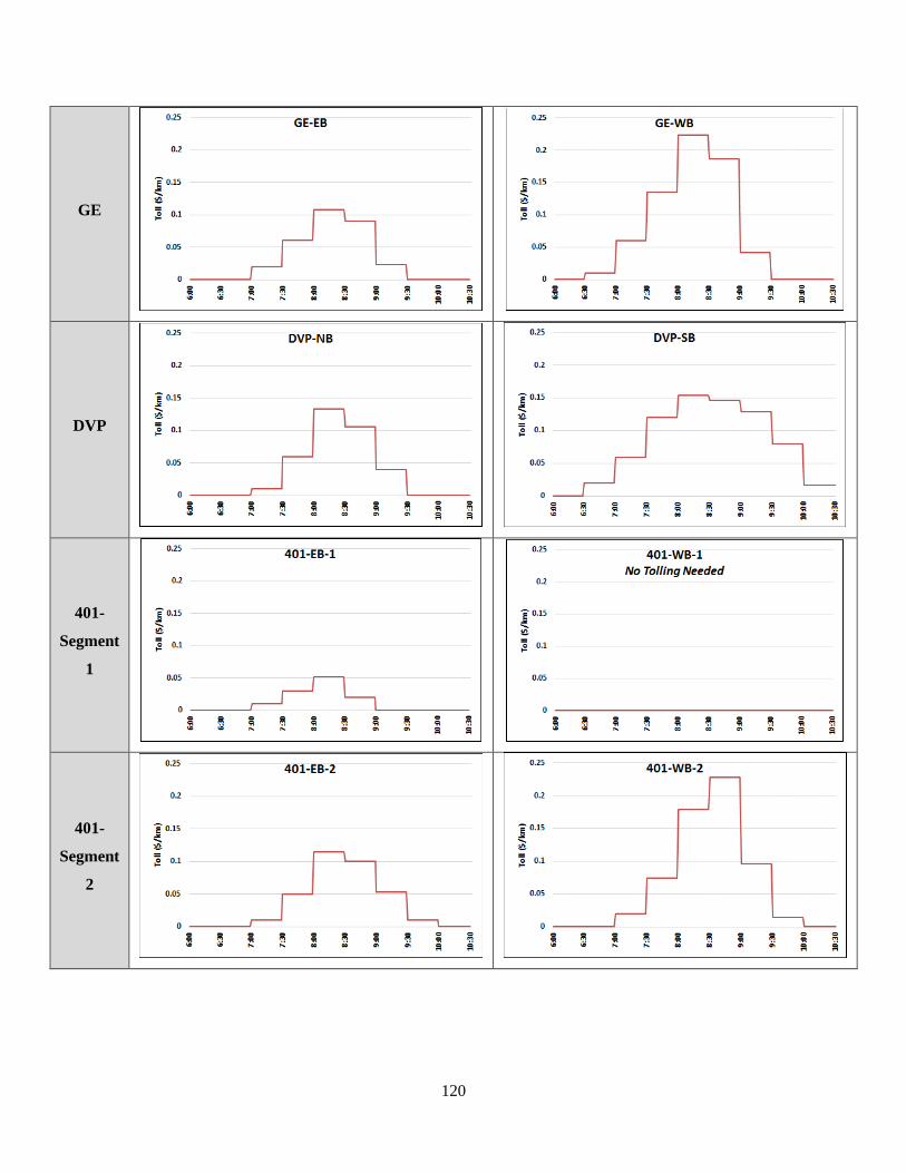
120

GE

DVP

401-

Segment

1

401-

Segment

2

121

401-

Segment

3

Network Performance Evaluation under Tolling Scenario II

The initial toll structures calculated are then applied to the corresponding routes and tested

through the integrated testbed of departure time and GTA DTA simulation models. The system

terminates when equilibrium is reached under the tolling scenario tested. Total travel times

network-wide decreased from 605690 hr to 601363 hr after tolling; i.e., 4327 hours were saved

in traffic during the 6:00 to 10:30 am period as a result of the initial toll structures imposed.

The improvement in total network travel times is minimal considering the fact that only 138

freeway km are tolled in this scenario, out of a total of 5727 km (1138 freeway km plus 4589

arterial km) modelled in the network. However, it indicates that the initial toll structures tested

did not exacerbate the total network performance due to possible longer alternative paths taken to

avoid tolls or increased traffic on non-tolled parallel arterials.

The 6:00 to 10:30 am period considered here involves less congested early and late intervals that

can realistically attract traffic as a consequence of variable tolling. In other words, the departure

time choice process – among different intervals – involves trade-offs between travel time cost,

schedule-delay cost, and toll cost. Figure 6-11 illustrates the departure time changes, across

different intervals, for the original 455,000 commuting trips travelling through tolled routes

and/or their parallel arterials in the morning period. Variable tolling prompted departure time

changes amongst trips that passed through tolled routes; they represent almost half the total

commuting trips considered. As is clear from the figure, around 4% of the total commuting trips

from the 7:30 am to 9:00 am peak period shifted to earlier and later intervals. Shifts to early

122

intervals are obviously higher than late intervals for the reason that the late arrival shadow price

is higher than that of early arrival, as highlighted before.

Figure 6-11: Percentage of Commuting Trips Shifted to/from each Time-Interval after Tolling

As mentioned before, the tolling schemes designed here have two main objectives. The first is to

induce proper route shifts resulting in better infrastructure utilization (i.e., higher flow levels) on

tolled routes and their parallel arterials. The second objective is to prompt traffic pacing –

through variable tolling – that works towards eliminating traffic queues on tolled routes, while

considering drivers’ captivity to their desired arrival times. In other words, the purpose of

congestion pricing is to enforce spatial and temporal traffic distribution for the sake of improved

infrastructure utilization and network performance (i.e., lower total travel times).

In light of these objectives, it is important to evaluate (i.e., measure) the impact of departure time

and route shifts – motivated by the tolling scenario – on tolled routes and their parallel arterials.

For that purpose, the travel time patterns of tolled routes are calculated, based on the output of

the tolling scenario, and compared against those estimated in the base-case, as will be illustrated

later. It should be noted, however, that travel times might not solely capture the utilization

efficiency of tolled routes and their parallel arterials. For instance, improved travel times due to

significantly decreased flow levels (i.e., underutilization of route capacity) are not desired.

Additionally, improved travel times on tolled routes together with increased congestion (hence

travel delays) on parallel arterials are not desired either. Accordingly, the number of route users

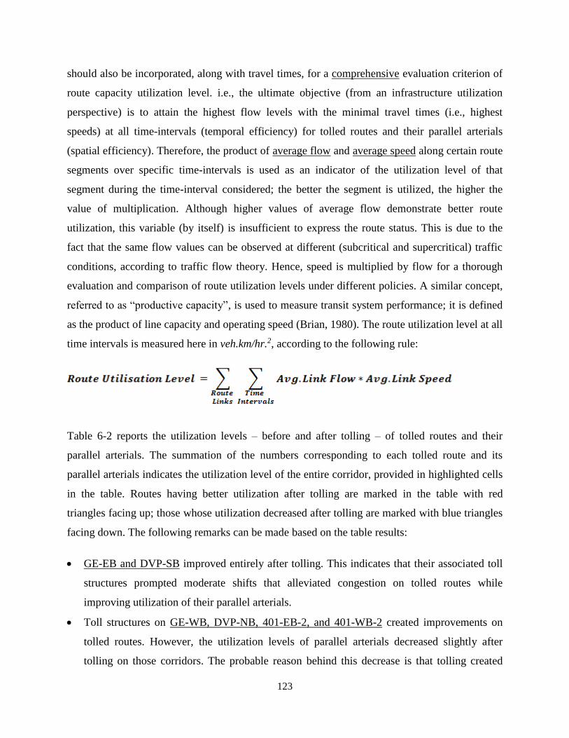
123

should also be incorporated, along with travel times, for a comprehensive evaluation criterion of

route capacity utilization level. i.e., the ultimate objective (from an infrastructure utilization

perspective) is to attain the highest flow levels with the minimal travel times (i.e., highest

speeds) at all time-intervals (temporal efficiency) for tolled routes and their parallel arterials

(spatial efficiency). Therefore, the product of average flow and average speed along certain route

segments over specific time-intervals is used as an indicator of the utilization level of that

segment during the time-interval considered; the better the segment is utilized, the higher the

value of multiplication. Although higher values of average flow demonstrate better route

utilization, this variable (by itself) is insufficient to express the route status. This is due to the

fact that the same flow values can be observed at different (subcritical and supercritical) traffic

conditions, according to traffic flow theory. Hence, speed is multiplied by flow for a thorough

evaluation and comparison of route utilization levels under different policies. A similar concept,

referred to as “productive capacity”, is used to measure transit system performance; it is defined

as the product of line capacity and operating speed (Brian, 1980). The route utilization level at all

time intervals is measured here in veh.km/hr.2, according to the following rule:

Table 6-2 reports the utilization levels – before and after tolling – of tolled routes and their

parallel arterials. The summation of the numbers corresponding to each tolled route and its

parallel arterials indicates the utilization level of the entire corridor, provided in highlighted cells

in the table. Routes having better utilization after tolling are marked in the table with red

triangles facing up; those whose utilization decreased after tolling are marked with blue triangles

facing down. The following remarks can be made based on the table results:

GE-EB and DVP-SB improved entirely after tolling. This indicates that their associated toll

structures prompted moderate shifts that alleviated congestion on tolled routes while

improving utilization of their parallel arterials.

Toll structures on GE-WB, DVP-NB, 401-EB-2, and 401-WB-2 created improvements on

tolled routes. However, the utilization levels of parallel arterials decreased slightly after

tolling on those corridors. The probable reason behind this decrease is that tolling created

124

traffic shifts beyond the remaining available capacity on the parallel arterials of those

corridors.

401-WB-3 and 401-EB-1 became underutilized after tolling. However, the utilization level of

their parallel arterials increased. This indicates that the initial toll structure of these routes

was relatively high, and that the parallel arterials had sufficient capacity to absorb the traffic

that had shifted after tolling.

Overall, the aggregate utilization levels of most of the corridors – reported in the highlighted

cells – improved after tolling. Moreover, the utilization level of all tolled routes along with their

parallel arterials improved after tolling, as can be concluded from the final record in the table.

The role of toll structure fine-tuning (i.e. the second level of optimal toll determination) is to

adjust the initial toll structures in order to attain the best utilization levels resulting in the

minimum total travel times network-wide, as will be detailed in the next chapter.

Table 6-2: Infrastructure Utilization Level (in veh.km/hr2) of Tolled Routes and their Parallel Arterials

before and after Tolling

Route Base-Case Under Tolling Scenario II

GE-EB (Tolled) 7.20 * 10^8 7.39 * 10^8 ▲

GE-EB (Parallel) 9.48 * 10^8 9.69 * 10^8 ▲

GE-EB (Corridor) 1.67 * 10^9 1.71 * 10^9 ▲

GE-WB (Tolled) 8.41 * 10^8 10.07 * 10^8▲

GE-WB (Parallel) 6.00 * 10^8 5.72 * 10^8 ▼

GE-WB (Corridor) 1.44 * 10^9 1.58 * 10^9 ▲

DVP-NB (Tolled) 8.37 * 10^8 8.45 * 10^8 ▲

DVP-NB (Parallel) 4.18 * 10^8 4.16 * 10^8 ▼

DVP-NB (Corridor) 1.25 * 10^9 1.26 * 10^9 ▲

DVP-SB (Tolled) 8.63 * 10^8 9.44 * 10^8 ▲

DVP-SB (Parallel) 5.55 * 10^8 5.56 * 10^8 ▲

DVP-SB (Corridor) 1.42 * 10^9 1.50 * 10^9 ▲

401-EB-1 (Tolled) 2.87 * 10^8 2.50 * 10^8 ▼

401-EB-1 (Parallel) 4.63 * 10^8 4.66 * 10^8 ▲

401-EB-1 (Corridor) 7.50 * 10^8 7.16 * 10^8 ▼

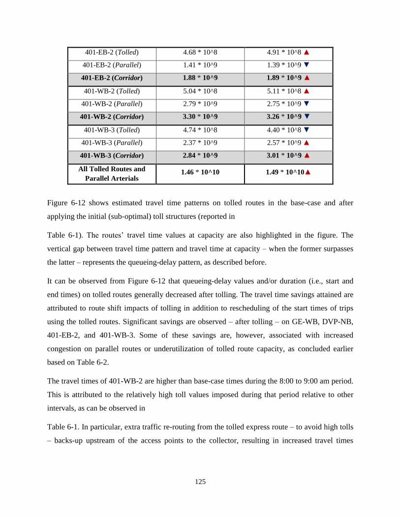
125

401-EB-2 (Tolled) 4.68 * 10^8 4.91 * 10^8 ▲

401-EB-2 (Parallel) 1.41 * 10^9 1.39 * 10^9 ▼

401-EB-2 (Corridor) 1.88 * 10^9 1.89 * 10^9 ▲

401-WB-2 (Tolled) 5.04 * 10^8 5.11 * 10^8 ▲

401-WB-2 (Parallel) 2.79 * 10^9 2.75 * 10^9 ▼

401-WB-2 (Corridor) 3.30 * 10^9 3.26 * 10^9 ▼

401-WB-3 (Tolled) 4.74 * 10^8 4.40 * 10^8 ▼

401-WB-3 (Parallel) 2.37 * 10^9 2.57 * 10^9 ▲

401-WB-3 (Corridor) 2.84 * 10^9 3.01 * 10^9 ▲

All Tolled Routes and

Parallel Arterials 1.46 * 10^10 1.49 * 10^10▲

Figure 6-12 shows estimated travel time patterns on tolled routes in the base-case and after

applying the initial (sub-optimal) toll structures (reported in

Table 6-1). The routes’ travel time values at capacity are also highlighted in the figure. The

vertical gap between travel time pattern and travel time at capacity – when the former surpasses

the latter – represents the queueing-delay pattern, as described before.

It can be observed from Figure 6-12 that queueing-delay values and/or duration (i.e., start and

end times) on tolled routes generally decreased after tolling. The travel time savings attained are

attributed to route shift impacts of tolling in addition to rescheduling of the start times of trips

using the tolled routes. Significant savings are observed – after tolling – on GE-WB, DVP-NB,

401-EB-2, and 401-WB-3. Some of these savings are, however, associated with increased

congestion on parallel routes or underutilization of tolled route capacity, as concluded earlier

based on Table 6-2.

The travel times of 401-WB-2 are higher than base-case times during the 8:00 to 9:00 am period.

This is attributed to the relatively high toll values imposed during that period relative to other

intervals, as can be observed in

Table 6-1. In particular, extra traffic re-routing from the tolled express route – to avoid high tolls

– backs-up upstream of the access points to the collector, resulting in increased travel times

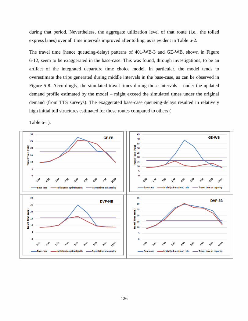
126

during that period. Nevertheless, the aggregate utilization level of that route (i.e., the tolled

express lanes) over all time intervals improved after tolling, as is evident in Table 6-2.

The travel time (hence queueing-delay) patterns of 401-WB-3 and GE-WB, shown in Figure

6-12, seem to be exaggerated in the base-case. This was found, through investigations, to be an

artifact of the integrated departure time choice model. In particular, the model tends to

overestimate the trips generated during middle intervals in the base-case, as can be observed in

Figure 5-8. Accordingly, the simulated travel times during those intervals – under the updated

demand profile estimated by the model – might exceed the simulated times under the original

demand (from TTS surveys). The exaggerated base-case queueing-delays resulted in relatively

high initial toll structures estimated for those routes compared to others (

Table 6-1).

127

Figure 6-12: Tolled-Routes’ Travel Time Patterns before and after Tolling

Concluding Remarks

The simple and extended tolling scenarios presented in this chapter show the effectiveness of the

proposed system in 1) determining initial (sub-optimal) toll structures for congested facilities,

following the Bottleneck Model dynamic pricing rules, 2) simulating the consequent travellers’

routes and departure time choice responses through integrated testbed of departure time and

DTA simulation models, and 3) evaluating the network performance under each scenario. The

tolling scenario evaluation criteria included travel time savings and route shift patterns network-

wide; the utilization level of tolled corridors (i.e. tolled routes and/or their parallel arterials);

travel time savings on tolled routes; and the impacts of tolling on travel times and departure time

choices of commuting trips affected by tolling.

The results demonstrate how congestion pricing on real-world road networks can have different

effects to those suggested by studies of single links or toy networks. For example, unlike the

simple Bottleneck Model, variable tolling affects not only the cumulative loading curve but also

128

the cumulative exit curve. Another example is that imposing a flat toll on a link can actually

increase travel time on the link because of spillback. The results also indicate the importance of

conducting simulations on a regional scale for policy determination and assessment. It can be

observed that benefits come from route shift impacts of tolling in addition to rescheduling of

departure times due to variable pricing, compared to re-routing only, as in flat tolling. This

affirms the necessity of integrating the departure time module into the congestion pricing system,

for realistic modelling of travellers' departure time responses to variable pricing policies.

Moreover, the comparisons conducted in the first scenario between flat and variable tolling

structures emphasize the importance of variable pricing to replicate congestion patterns over

time; otherwise, tolling might bring counterproductive results.

In conclusion, the initial toll structures determined via the “first level of optimal toll

determination” module resulted in noticeable overall benefits – at different levels – in both

scenarios. However, further adjustments are needed for the toll levels of those (initial) structures

to optimize the utilization level of tolled corridors (and hence to avoid the undesired impacts of

tolling) and minimize total travel times network-wide. The toll adjustment (fine-tuning) process

considers the interconnectivity among tolled and non-tolled facilities in the network. The process

is achieved through a distributed genetic optimization algorithm, as will be described in detail in

the next chapter.

129

7. Optimal Congestion Pricing Determination - Level II: Toll

Structures Fine-Tuning Using Distributed Genetic Optimization

Algorithm

This chapter describes the final module in the proposed optimal congestion pricing system

(outlined in Figure 3-1): the “Optimal Toll Determination – Level II”. The chapter starts with a

description of the different components of the optimization problem; e.g., the selected

optimization variables and objective function. An overview is then given of the genetic

optimization algorithm used and the choice of its parameters. After that, the middleware

integrated into the optimization platform for distributed computing is described along with the

configuration process conducted for the parallel cluster used. The optimization module is then

applied on the second tolling scenario – introduced in Chapter 6 – to optimize the initial toll

structures obtained for its eight tolled routes. Then, a comprehensive comparative assessment is

provided for the same scenario under different situations: base-case, initial toll structures, and

fine-tuned toll structures. The chapter concludes with a cost-benefit analysis provided to

investigate the implementation feasibility of the variable tolling strategies determined via the

proposed optimal congestion pricing system. .

7.1. Optimization Problem Description

7.1.1. Optimization Variables

As emphasized in Chapter 6, the initial toll structures derived replicate the base-case queueing-

delay patterns (defined as the excess travel time over ‘travel time at capacity’) of tolled facilities.

In other words, the tolling structure start and end times as well as toll values at different intervals

mirror the congestion temporal profile of the tolled route in the base-case. This is expected to

motivate departure time rescheduling (i.e., traffic pacing) towards eliminating queueing-delays

(i.e., hyper-congestion), according to the Bottleneck Model findings. Therefore, as a first

implementation, the variable selected to be controlled through optimization – for each tolled

route – is the magnitude of the toll structure of that route. Braid (1996) suggested adjusting the

optimal (first-best) toll structure on a bottleneck via shifting it up or down by a uniform amount,

when a second un-tolled bottleneck runs parallel to it. This approach might, however, lead to

130

tolling before the network reaches capacity; i.e. tolls may start earlier and stay later than the

bounds of the peak (during which queues exist in the unpriced equilibrium). It might also cause

the tolls to lose proportionality to congestion at different intervals, since adding equal amounts to

the numerator and denominator of a fraction will generally change its value. Accordingly, the

initial toll structure of each tolled route is adjusted during the toll fine-tuning process via

multiplying (rather than adding) it by certain factor. In other words, the entire structure is scaled

up or down by this factor, while preserving its start and end times and the relative ratios between

toll values at different intervals that were carefully estimated in the first level of optimal toll

determination based on the base-case queueing-delay patterns, as detailed in Chapter 6.

Accordingly, each tolled route considered will be assigned an optimization variable, i.e., a scale

factor (SF). The same SF is multiplied by all toll values corresponding to different intervals of

the initial toll structure of each route. Hence, the number of optimization variables (i.e. scale

factors) equals the number of tolled routes considered in the tolling scenario. For instance, the

second tolling scenario requires eight optimization variables for its eight tolled routes: SFGE-EB,

SFGE-WB, SFDVP-NB, SFDVP-SB, SF401-EB-1, SF401-EB-2, SF401-WB-2, and SF401-WB-3. Scale factors are real

numbers lying within a range from zero up to a maximum, set individually for each route, based

on its maximum allowable toll value. Each set of feasible values for the eight scale factors is

referred to as a “solution vector”.

7.1.2. Objective Function

The purpose of the “bi-level” procedure of optimal toll determination is to find the optimal toll

structures resulting in the best traffic distribution over space and time that alleviates congestion

(i.e., queueing-delay) on busy routes and time-intervals, respectively, and hence minimizes the

total travel times while accounting for commuters’ schedule-delay costs. As clarified earlier, the

first level of optimal toll determination entails the determination of initial (sub-optimal) toll

structures on each congested facility individually to eliminate queueing without considering the

effects on other routes. The initial toll structures are determined based on the Bottleneck Model

general pricing rules, which work towards eliminating queueing-delay on the congested facility,

through departure time rescheduling, while considering schedule-delay costs. The role of the

second level of optimal toll determination is to adjust the toll magnitudes of the initial toll

structures in order to maximize the utilization level of tolled corridors (i.e. tolled routes and their

131

parallel arterials) through route shifts, which will probably minimize the total travel times

network-wide (i.e., achieve system optimal (SO) traffic conditions).

The “total travel times network-wide” are produced and reported, as a single value, in the output

of the DTA simulation model. On the other hand, the “utilization level of tolled corridors” is

measured here by summing the multiplication of average flow and average speed over all links

(belonging to the tolled routes and their parallel arterials) at all time-intervals, as illustrated in

Chapter 6. The first criterion (i.e., the total travel times network-wide) is selected as an objective

function for the sake of inclusive assessment that involves the impact of scale factors (being

tested during optimization) not only on the tolled corridors but also on the entire network. The

second criterion (i.e., the utilization level of tolled corridors) is then used, after termination of the

optimization algorithm, to choose among the best solutions obtained in the last iteration

(exhibiting similar low total travel times). The purpose of doing this is to choose the best

solution that achieves not only improved travel times network-wide (which are directly

minimized during optimization), but also enhanced utilization efficiency of tolled corridors.

7.1.3. Optimization Problem Segmentation

In the case of a large number of tolled routes (hence optimization variables), the optimization

algorithm might encounter a quasi-flat objective function issue. i.e., the objective function takes

close values at various solution vectors tested during optimization, which makes the search

process for the global optimal solution extremely challenging and time-consuming. This

phenomenon has been observed when attempting to optimize the eight scale factors of the second

tolling scenario experiment concurrently. The main reason identified behind this issue is that, for

a general solution vector, the combined improvements and deteriorations observed on different

tolled routes – in response to their modified toll structures – might cancel each other out,

resulting in similar objective function values for various solution vectors. The issue becomes

more obvious as the number of tolled routes increases, especially if these routes (or some of

them) are not highly correlated; i.e., improvement or deterioration in traffic conditions of some

route causes no (or negligible) consequences on other routes. For instance, an accident on GE-

EB does not directly affect traffic conditions on 401-WB; however, it might partially block

access to DVP-NB shortly after its occurrence, and so on.

132

In fact, the issue described above might generally occur when attempting to optimize several

traffic policies, applied on barely correlated parts of the network, in one optimization process

(i.e., through a single objective function). More specifically, the individual impact of each tested

policy becomes diluted in the total objective function value that is affected by changes associated

with all policies tested. i.e., a single objective function value might not clearly reflect the

individual (positive or negative) local impacts of various policies tested under the same solution

vector.

In optimization theory, if a function of a certain system (e.g., total travel times network-wide) is

completely additive of the functions of its subsystems (travel times on separate parts/corridors)

and if these functions are independent of each other, then the function of the entire system is

optimized (i.e. minimized) when each function of its subsystems is optimized (Huang et al.,

2009). Accordingly, in order to address the quasi-flat objective function issue, toll structures

(i.e., scale factors) of each group of correlated routes are optimized separately, while fixing toll

structures of other tolled routes. That is, the optimization problem is separated into smaller

problems to avoid the quasi-flat – that is, hard to be optimized – objective function associated

with a larger number of (uncorrelated) tolled routes. Another benefit achieved through this

problem segmentation comes from the fact that the smaller the number of optimization variables,

the faster the corresponding optimal solution can be reached under certain limited available

computational resources. This is of great significance in the current application given its large-

scale nature, entailing huge memory and computational time requirements, as highlighted before.

It should be mentioned that the full GTA simulation model is executed throughout all

calculations associated with small optimization problems. It should also be noted that according

to this theorem, the “total travel times network-wide” achieved under the optimal scale factors –

determined through several optimization problems – should theoretically take the same optimum

value obtained if all scale factors are optimized concurrently.

It is therefore necessary to set a proper criterion that can be used to quantify correlation among

different routes, and hence differentiate those whose toll structures can be optimized separately.

Intuitively, as the amount of common traffic using certain routes increases, the mutual impact

between traffic conditions on those routes increases as well. Accordingly, the ‘correlation level’

between two routes is measured here based on the percentage of their common traffic with

133

respect to the average traffic using both routes. The former quantity denotes the trips passing

through both routes; the latter refers to the average number of ‘distinct’ trips using any of the two

routes. The correlation level calculation approach is further illustrated in the following formula.

The number of common trips is subtracted in the denominator to avoid double counting them.

The number of common trips and the correlation level among each couple of routes – selected to

be tolled in the second scenario – are displayed in the matrix presented in Table 7-1. A number

displayed in the matrix diagonal (i.e., having the same row and column IDs) represents the total

number of trips passing through the route associated with its row/column, in the base-case during

the morning analysis period considered in this study. On the other hand, a general number

displayed in row X and column Y represents the number of common trips among routes X and Y.

Moreover, the correlation levels among different routes, calculated based on the preceding

formula, are displayed in brackets in the same matrix. Obviously, the matrix is symmetrical;

therefore, only one half of it is given in the table.

A threshold value of 10% is set to identify correlated routes. That is, two routes are considered to

be correlated if their correlation level exceeds the threshold value set. The cells corresponding to

the correlated route pairs – determined based on this criterion – are highlighted in the lower half

of the matrix.

The next step after identifying correlated route pairs is to cluster each group of mutually

correlated routes whose toll structures can be optimized separately. This is performed through

the algorithm illustrated in Figure 7-1. According to that algorithm, three groups of mutually

correlated tolled routes are identified for the second tolling scenario as follows:

1. GE-EB and DVP-NB.

2. 401-WB-3, 401-WB-2, DVP-SB, and GE-WB.

3. 401-EB-1 and 401-EB-2.

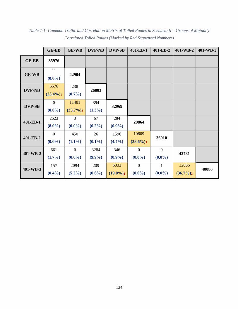
134

Table 7-1: Common Traffic and Correlation Matrix of Tolled Routes in Scenario II – Groups of Mutually

Correlated Tolled Routes (Marked by Red Sequenced Numbers)

GE-EB GE-WB DVP-NB DVP-SB 401-EB-1 401-EB-2 401-WB-2 401-WB-3

GE-EB 35976

GE-WB 11

(0.0%) 42904

DVP-NB 6576

(23.4%)1

238

(0.7%) 26883

DVP-SB 0

(0.0%)

11481

(35.7%)2

394

(1.3%) 32969

401-EB-1 2523

(8.0%)

3

(0.0%)

67

(0.2%)

284

(0.9%) 29864

401-EB-2 0

(0.0%)

450

(1.1%)

26

(0.1%)

1596

(4.7%)

10809

(38.6%)3

36910

401-WB-2 661

(1.7%)

0

(0.0%)

3284

(9.9%)

346

(0.9%)

0

(0.0%)

0

(0.0%) 42781

401-WB-3 157

(0.4%)

2094

(5.2%)

209

(0.6%)

6332

(19.0%)2

0

(0.0%)

1

(0.0%)

12856

(36.7%)2

40086

135

Figure 7-1: Algorithm for Clustering Mutually Correlated Routes

In fact, the approach presented in this section to identify the correlated routes/parts of the

network can also be employed for other traffic planning purposes. For instance, if some

‘existing’ traffic policies undergo major operational changes/upgrades, it might be important to

determine whether or not other ‘existing’ policies need to be altered accordingly in order to

avoid undesired consequences on other parts of the network. This can be achieved by analyzing

the correlation between the areas of influence of different policies according to the criterion

presented, and so on.

7.2. The Optimization Methodology – Distributed Genetic Algorithm

7.2.1. Genetic Algorithms: Overview and Parameter Design

A Genetic Algorithm (GA) is utilized here to find the optimal scale factors for the initial toll

structures, resulting in the best network performance. GAs are heuristic search approaches that

avoid most of the problems associated with traditional deterministic optimization techniques

(e.g., gradient descent approaches, the simplex method, and the Frank-Wolfe algorithm). More

{ //start

For (each column in the matrix)

{

For (each row in that column)

{

If (route is correlated with route )

{

If (route or belongs to a previously formed cluster )

{

Add the other route to cluster .

}

Else

{

Form a new cluster and add routes and to it.

}

}

}

}

} //end

136

specifically, GAs rely on the evolution of multiple solutions in the search space; therefore, they

have higher chances of finding the global optima without getting stuck in local minima (or

maxima). Additionally, GAs do not require differentiation of the objective function, which is

suitable for problems in which the objective function cannot be represented in a closed form

(such as the current application). Moreover, an important property of GAs is that they can be

parallelized (Back, 1996). That is, the evaluation of different solutions (chromosomes) can be

distributed across multiple processing units simultaneously. This allows the power of High

Performance Computing (HPC) clusters to be employed in large-scale – memory and

computationally demanding – applications.

GAs are inspired by the process of natural selection and biological evolution. In a GA, a

population of initial solutions (chromosomes) is first created. A chromosome is one feasible

point in the search space; it carries the values of the optimization variables in the form of a string

of genes. Each candidate solution (i.e. chromosome) in the population is then evaluated to obtain

some measure of its ‘fitness’. Evaluation can be as simple as substituting variable (gene) values

in a closed-form mathematical function, if one exists, or it might require a series of long

simulation runs such as the current application. After evaluating the fitness values of initial

chromosomes, selection and a series of genetic operators (crossover and mutation) are applied on

the population to produce new candidate solutions (i.e. children), with increasingly improved

fitness values. In each generation, fitter chromosomes have higher probabilities of being selected

for reproduction; hence the stochastic gradual improvement in fitness from one generation to the

next. This cycle of evaluation, selection, and reproduction continues for a number of generations

(iterations) until a certain stopping criterion is met.

In the current application, the genes represent the values of the scale factors corresponding to the

tolled routes under consideration in each optimization problem, as will be specified in detail

later. Moreover, the ‘fitness’ value of each chromosome is measured directly through the

objective function value (i.e., the total travel times network-wide) attained under this

chromosome. Figure 7-2 is a close-up of the “Optimal Toll Determination – Level II” module

integrated into the full system (Figure 3-1). The figure illustrates the basic GA cycle executed

within this module.

137

As clarified in the figure, the module takes as input the initial (sub-optimal) toll structures of

congested facilities, determined in the 1st level of optimal toll determination. The genes (scale

factors) tested during optimization are multiplied by the initial toll structures of the

corresponding facilities, as highlighted earlier. As outlined in the figure, the GA utilized in the

module goes through the following cycle:

– Initial population: generates random initial chromosomes within the solution search

space. The initial chromosomes are generated to be uniformly distributed across the

solution space in each problem. This is to avoid trapping the GA within a limited search

domain, and to guarantee obtaining a global optimal solution through exploring diverse

spots in the solution space during evolution.

– Fitness evaluation: evaluates fitness values of chromosomes in the population through

the integrated testbed of departure time choice and DTA simulation models, described in

earlier chapters. Specifically, the genes (scale factors) of each chromosome are multiplied

by the initial toll structures. The new toll structures are then entered as input to the

integrated departure time choice and DTA simulation models. The chromosome fitness

value is calculated as the total travel times network-wide obtained after equilibrium in

route and departure time choices.

– Selection: chooses the best candidate solutions to pass their genetic information from one

generation to the next based on their fitness values. Therefore, individuals with higher

fitness values have a greater chance to be copied to the intermediate population for the

genetic operators to exchange their traits for better solutions. Specifically, a “ranking

selection” mechanism is used here, in which individuals in a population of n

chromosomes are ranked in descending order of fitness, with a rank of n points given to

the best individual and a rank of 1 given to the worst individual. Roulette wheel selection

is then performed based on the probability calculated according to the individual rank as

follows (Mohamed, 2007):

“Ranking selection” will tend to avoid premature convergence by tempering selection

pressure for large fitness differentials that occur in early generations. This is due to

138

calculating the probability of selection for each individual based on its ranking, and not

the fitness value.

– Reproduction: applies genetic operators of crossover and mutation on the selected

intermediate population to generate new candidate solutions:

o Crossover: acts on two parents in the intermediate population by combining their

traits (genetic information) to form two new children. This operator is applied

with a probability denoted as the crossover probability; it is assigned a value of

0.9 in this study.

o Mutation: randomly changes each allele in every chromosome in the population

based on the mutation probability selected. It is considered as a secondary

operator in order not to lose the fittest potential areas in the search space;

therefore, the probability of mutation should be small. It is assigned a value of

0.05 in this study.

– New generation: chooses the best (i.e. fittest) chromosomes out of the current generation

and the reproduced children for the new generation.

– Convergence: the cycle described is repeated until a pre-specified convergence criterion

is met, as will be clarified later. The convergence sought at this step represents the third

and highest level of convergence (i.e., the toll structure convergence) in the optimal

congestion pricing system.

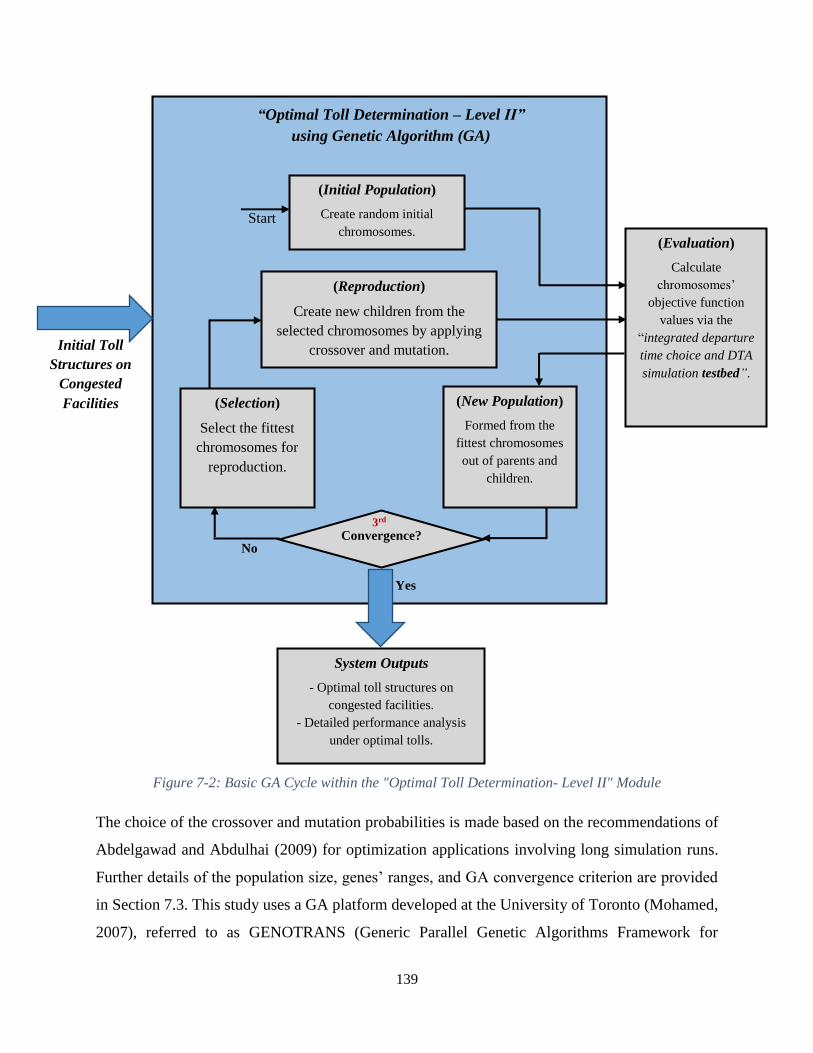
139

Figure 7-2: Basic GA Cycle within the "Optimal Toll Determination- Level II" Module

The choice of the crossover and mutation probabilities is made based on the recommendations of

Abdelgawad and Abdulhai (2009) for optimization applications involving long simulation runs.

Further details of the population size, genes’ ranges, and GA convergence criterion are provided

in Section 7.3. This study uses a GA platform developed at the University of Toronto (Mohamed,

2007), referred to as GENOTRANS (Generic Parallel Genetic Algorithms Framework for

(Evaluation)

Calculate

chromosomes’

objective function

values via the

“integrated departure

time choice and DTA

simulation testbed”.

System Outputs

- Optimal toll structures on

congested facilities.

- Detailed performance analysis

under optimal tolls.

(Initial Population)

Create random initial

chromosomes.

(Reproduction)

Create new children from the

selected chromosomes by applying

crossover and mutation.

(Selection)

Select the fittest

chromosomes for

reproduction.

(New Population)

Formed from the

fittest chromosomes

out of parents and

children.

Convergence?

“Optimal Toll Determination – Level II”

using Genetic Algorithm (GA)

Initial Toll

Structures on

Congested

Facilities

Start

Yes

No

3rd

140

Optimizing Intelligent Transportation Systems). The distributed GA feature in GENOTRANS

was upgraded by integrating and configuring a Java-based middleware for distributed in-memory

processing, denoted as Apache Ignite. This upgrade resulted from the collaborate teamwork of

Tamer Abdulazim, Islam Kamel, Mohamed Elshenawy and the author. Not only can

computations be carried out concurrently on parallel processing units, but also the system

deployment on a large network of remote servers – hosted on the Internet – is made possible

through this platform upgrade. This eliminates the need for a local physical computing cluster,

and allows on-demand access to Internet-based shared resources based on the application

requirements. The configuration and implementation details relevant to the integrated

middleware are detailed next.

7.2.2. Distributed Computing Configuration and Implementation

As can be inferred from the details provided so far, the system implementation involves

integration and iteration among several large-scale computationally intensive modules, dealing

with (i.e., reading and writing) large amounts of input and output data. This entails storage issues

and unreasonably long system running times if only one computer is used. Accordingly, it

becomes necessary to harness the power of several computers in the system deployment.

For that reason, the GA is run concurrently on a parallel computing cluster managed through the

Apache Ignite middleware integrated to the optimization platform. The middleware operates

under a Map-Reduce programming paradigm that orchestrates the processing by controlling the

distributed servers, running the various tasks in parallel, and managing all communications and

data transferred between different system components, while avoiding redundancy (Dean and

Ghemawat, 2004). In particular, several solutions (chromosomes) are distributed (mapped) to

multiple nodes of the cluster and evaluated in parallel, i.e. each node (CPU) evaluates one

chromosome. The evaluation results are then combined (reduced) at the master node for further

processing. A new batch of solutions is subsequently mapped/reduced, and so on until the

optimization algorithm reaches equilibrium.

It is important to note that there are two main strands of distributed computing applications:

Massive Parallel Processing (MPP) and High-Performance Computing (HPC). MPP involves

breaking the program into relatively small tasks distributed over a massive number of nodes.

141

HPC is the use of parallel processing for running advanced (memory and computationally

demanding) application programs efficiently, reliably and quickly. In other words, HPC is likely

to be employed for complex applications requiring high processing power and speed (Rouse,

2007). In the optimal congestion pricing application, the individual tasks (chromosome fitness

calculation) involve running a series of long simulation runs iteratively with the departure time

choice model. Therefore, the application can be classified under the second strand, which

requires a HPC parallel cluster.

In general, the two described strands require different configuration settings of the distributed

computing engine. For example, the “failure detection time-out” is one of the configuration

parameters to be selected. This represents the maximum allowable time, beyond which the task

being executed on some node is aborted if that node does not respond to the other cluster nodes

within the preset allowable time span. This parameter should therefore be assigned smaller

values in MPP applications compared to HPC applications. This is because the frequency of

communication and data transfer between cluster nodes in the former applications is generally

higher than the latter, due to the short running-time of their parallel tasks. i.e., setting a small

“failure detection time-out” guarantees that a disconnected node in MPP applications is quickly

discovered and hence re-assigned a new task, for efficient use of cluster nodes.

The configuration process of a parallel cluster might require significant testing to find the proper

combination of parameters for the application under consideration. In fact, this was one of the

most challenging tasks in the current study, which involved several non-trivial issues. For

example, frequent disconnections of cluster nodes have been observed to occur shortly after the

DTA simulation model invokes the vehicle assignment module, denoted as MIVA

(Multithreaded Isochronal Vehicle Assignment). The reason identified for this phenomenon,

after extensive trials and investigations, is that when MIVA is started, the processor becomes

100% occupied for quite a long time (15–20 minutes) such that it does not respond to the master

node within the default time span value, and hence loses communication with the cluster.

Among the multiple solution tactics examined, two configurable parameters were found to tackle

this problem: the “failure detection time out” and the “maximum missed heartbeats”. These two

parameters control the maximum allowable response time, beyond which a node is considered

disconnected from the cluster if it does not respond to the master node messages. Accordingly,

142

the values of both parameters were relaxed such that the maximum allowable time span exceeds

the maximum execution period of MIVA (during which the processor might not communicate

properly with the cluster). Additionally, the number of processor cores allowed to be used by the

DTA simulation model in each node was set to be less than the total available cores in that node.

This is to avoid occupying the full processor for long time periods in a way that might affect the

communication exchanged between different cluster nodes.

As mentioned, each chromosome fitness calculation requires a considerable amount of memory

and processing power. Therefore, the configuration parameters related to the “number of parallel

jobs” were adjusted in order to guarantee that a new task (i.e., chromosome fitness calculation) is

started on certain node only after the execution of the preceding task has terminated on that node.

On the other hand, the memory required by the Java processes on different nodes varies

depending on the tasks assigned to these nodes. For example, the Java process in the master node

requires more memory than the other cluster nodes, due to the communication overheads

associated with it. Accordingly, the “maximum memory allocated to Java” was one of the

parameters configured in this study, upon several trials, to avoid having failures related to the

limited Java space.

As emphasized earlier, an important feature of integrated Java-based middleware is that it

enables the deployment of the optimal congestion pricing system on a network of remote servers

hosted on the Internet. This makes the use of online shared memory and computing resources

possible, depending on the requirements of the application under consideration. In other words, it

eliminates the system dependency on a certain physical (local) parallel computing cluster.

As a first implementation, a parallel cluster of five computers – each having 16 GB of RAM

memory and Intel Core i7-3770 processor @ 3.40 GHz – was made available in the Intelligent

Transportation Systems Laboratory at the University of Toronto, to test and implement the

optimal congestion pricing system on simulation-based case studies in the GTA. In the future,

subject to available financial resources, we may consider running the system on commercially

available HPCs, such as those offered by Amazon and others.

143

7.3. Full Optimal Congestion-Pricing System Implementation Results and

Analysis for Tolling Scenario II

This section presents the implementation details and results of applying the “second level of

optimal toll determination” on tolling scenario II considered for the GTA region. This step

concludes the full optimal congestion pricing system implementation for that tolling scenario.

As clarified in Section 7.1, the optimization of the scale factors to be multiplied by the initial

(sub-optimal) toll structures of the eight tolled routes in the second scenario, is carried out

separately for each group of correlated routes. Accordingly, the distributed GA optimization

module is applied separately and sequentially for three optimization problems classified in Table

7-2.

While optimizing the toll structures of specific routes in each problem, those of other tolled

routes are kept fixed to their initial values or to their optimized values (if already obtained in

preceding problems), as indicated in the 4th column of Table 7-2. This setting guarantees that the

impact of the optimized toll structures is considered during subsequent optimization problems.

Moreover, the sequence of carrying out the three optimization problems is ordered such that the

one having the largest number of optimization variables is conducted at the end, as highlighted in

the table, to avoid altering its optimum results during subsequent problems. Additionally, the

impact of previously optimized toll structures – on the utilization levels of their corridors – is re-

evaluated in subsequent optimization problems. This is to ensure that altering (i.e., optimizing)

the tolls of other routes does not affect the best route utilization levels attained under previously

optimized toll structures.

The population size, the genes’ feasible ranges, and the stopping criterion are among the GA

parameters to be designed for a particular application. It should be noted that there is tradeoff in

any optimization technique, involving multiple initial solutions, between the number of initial

solutions (i.e., the population size in a GA) and the number of generations required until

convergence (i.e., the speed of convergence). In some cases, however, the GA might get stuck at

a local minimum if it starts the search process from a limited number of initial solutions,

regardless of the number of generations produced. This is because the new chromosomes –

produced though the genetic operators of crossover and mutation – evolve within a limited area

144

in the search space. Therefore, other potentially better areas in the search space might not be

explored.

Table 7-2: Optimization Problems’ Specifications for Tolling Scenario II

Chromosome

Size

Optimization Variables

(Genes)

Toll Structures on

other Routes

Population

Size

Optimization

Problem 1 2

Gene 0:

Gene 1:

401-EB-1 Initial

16

401-EB-2 Initial

401-WB-3 Initial

401-WB-2 Initial

GE-WB Initial

DVP-SB Initial

Optimization

Problem 2 2

Gene 0:

Gene 1:

GE-EB Optimal

10

DVP-NB Optimal

401-WB-3 Initial

401-WB-2 Initial

GE-WB Initial

DVP-SB Initial

Optimization

Problem 3 4

Gene 0:

Gene 1:

Gene 2:

Gene 3:

GE-EB Optimal

10

DVP-NB Optimal

401-EB-1 Optimal

401-EB-2 Optimal

The population size is generally recommended to be larger than the chromosome size (i.e., the

number of genes). As reported in Table 7-2, a population size equal to 16 was selected in the first

optimization problem. This value was however cut to 10 in the following two problems for the

sake of more efficient utilization of the available computers in the parallel cluster. In particular,

if the population size is not a multiple of the cluster size, then some nodes will be occasionally

idle during the fitness evaluations of the population chromosomes.

145

The genes (i.e. scale factors) are specified in this application as real numbers with a minimum

allowable value equal to zero. The maximum allowable value for each gene is determined based

on the evaluation results of the initial toll structure corresponding to that gene. That is, lower

maximum limits were assigned to the scale factors corresponding to overestimated initial toll

structures (e.g. 401-EB-1 and 401-WB-3), and vice versa. The purpose of doing this is to limit

the search space to areas beyond which toll structures might be excessively high, and would

hence result in undesired (counterproductive) results, or might be politically unpalatable with

consequent public disapproval. In other words, the lessons learned from the evaluation results of

the initial (sub-optimal) toll structures are harnessed to provide the GA with a concise search

space for a faster and more efficient evolution/search process. The upper limits of different genes

were assigned values ranging from 1–3.

The optimization process is terminated if the value of the best fitness function does not change

by more than 1% (over two successive generations) or if the number of iterations reaches 10;

whichever comes first.

7.3.1. GA Evolution and Optimal Solutions

Figure 7-3 illustrates the GA evolution results of the three optimization problems and the optimal

solution achieved in each case after convergence. As can be observed from the figure, the first

two problems converge after three generations, whereas the third converges after six generations

(obviously due to its larger chromosome size). The worst (highest) fitness values decrease among

successive generations, while the best (lowest) values converge to certain minimal (optimal)

value. As mentioned before, further comparisons are conducted between the best (candidate)

solutions obtained in the final GA iteration, in order to choose the solution that achieves not only

improved travel times network-wide (directly optimized through the GA), but also enhanced

utilization efficiency of the tolled corridors. The comparisons depend on the utilization levels

attained on the tolled corridors corresponding to the tolled routes being optimized in each

problem.

The convergence observed in different optimization problems is relatively fast, considering the

large-scale nature of the application. Specifically, a total of 12 GA iterations were performed

over the three optimization problems until convergence, as opposed to 25 iterations performed in

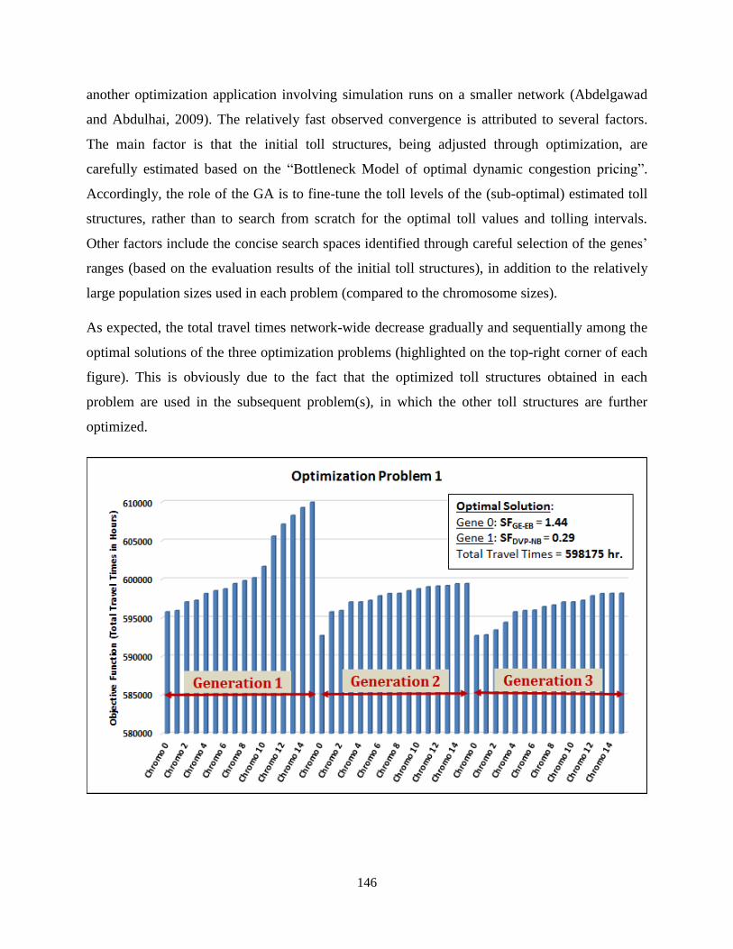
146

another optimization application involving simulation runs on a smaller network (Abdelgawad

and Abdulhai, 2009). The relatively fast observed convergence is attributed to several factors.

The main factor is that the initial toll structures, being adjusted through optimization, are

carefully estimated based on the “Bottleneck Model of optimal dynamic congestion pricing”.

Accordingly, the role of the GA is to fine-tune the toll levels of the (sub-optimal) estimated toll

structures, rather than to search from scratch for the optimal toll values and tolling intervals.

Other factors include the concise search spaces identified through careful selection of the genes’

ranges (based on the evaluation results of the initial toll structures), in addition to the relatively

large population sizes used in each problem (compared to the chromosome sizes).

As expected, the total travel times network-wide decrease gradually and sequentially among the

optimal solutions of the three optimization problems (highlighted on the top-right corner of each

figure). This is obviously due to the fact that the optimized toll structures obtained in each

problem are used in the subsequent problem(s), in which the other toll structures are further

optimized.

147

Figure 7-3: GA Evolution and Optimal Solutions of the Three Optimization Problems

148

An interesting observation from the evaluation analysis of various chromosomes generated

during optimization is that the tolled corridors have different sensitivities to identical toll

changes on their tolled routes. That is, the same amount of toll increase (or decrease) might lead

to different results on tolled routes and their parallel arterials, depending on the corridor

criticality (i.e., usage level) and the available capacity of parallel arterials. For instance, a small

toll increase (i.e. a few cents per km) on the GE-EB above the optimal levels can send excessive

traffic to off-ramps to parallel routes, such that it blocks the off-ramp and backs up onto the main

freeway. On the other hand, significant toll changes (up to 15 cents per km) on the lower section

of the DVP-NB (south of Bloor Street) hardly affect the total travel times and utilization level of

the entire corridor. This emphasizes the importance of conducting tolled route-based analysis,

while considering the parallel arterials and the entire corridor vitality within the network.

Table 7-3 shows the execution times of the three optimization problems, corresponding to the

population size identified and the number of generations created in each problem until

convergence. The expected execution times if the system is implemented in a serial mode (i.e.,

using a single computer) are also provided in the table for comparison purposes and to show the

speedup achieved through the parallel cluster.

Table 7-3: GA Execution Time under Serial and Parallel Modes

Population

Size

# of

Generations

Execution Time

(Parallel Mode)

Execution Time

(Serial Mode)

Optimization

Problem 1 16 3 198 hours (8.25 days) 828 hours (5 weeks)

Optimization

Problem 2 10 3 108 hours (4.5 days) 450 hours (2.7 weeks)

Optimization

Problem 3 10 6 216 hours (9 days) 972 hours (6 weeks)

Total -- -- 522 hours (22 days) 2250 hours (3 months)

The optimal (fine-tuned) toll structures obtained from the three consecutive optimization

problems are illustrated in Table 7-4, along with their corresponding initial toll structures. The

optimal toll structures are calculated via multiplying the optimal scale factors (reported between

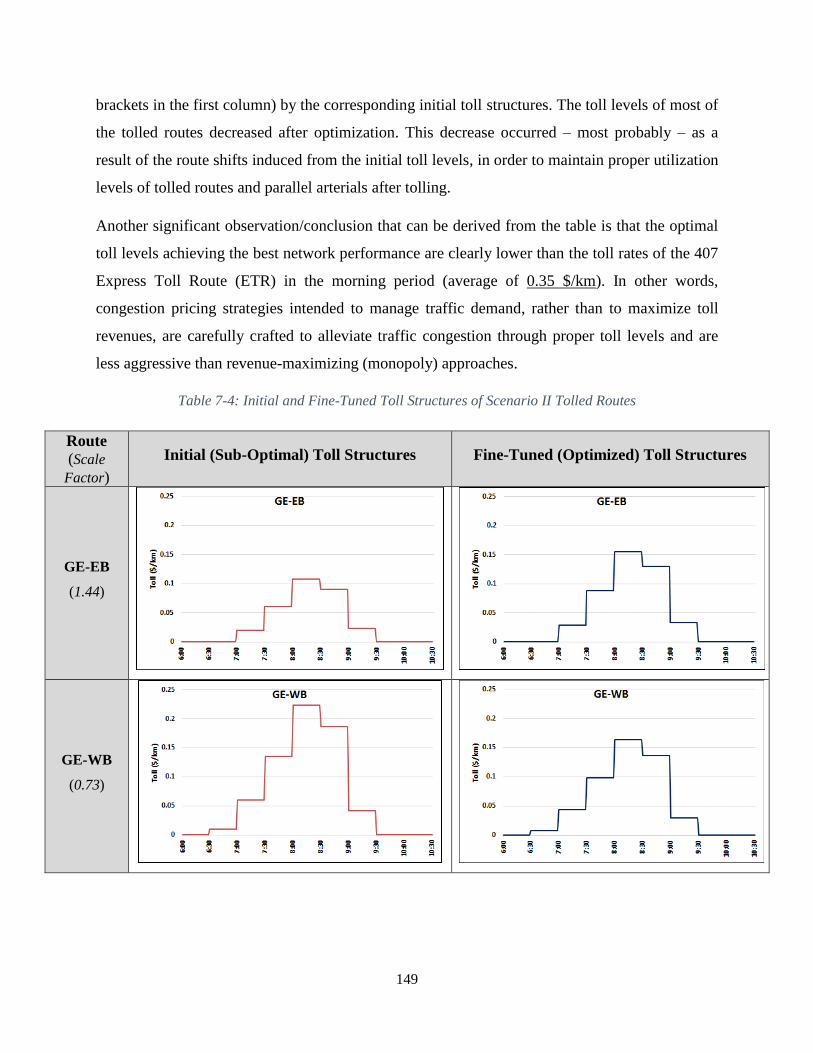
149

brackets in the first column) by the corresponding initial toll structures. The toll levels of most of

the tolled routes decreased after optimization. This decrease occurred – most probably – as a

result of the route shifts induced from the initial toll levels, in order to maintain proper utilization

levels of tolled routes and parallel arterials after tolling.

Another significant observation/conclusion that can be derived from the table is that the optimal

toll levels achieving the best network performance are clearly lower than the toll rates of the 407

Express Toll Route (ETR) in the morning period (average of 0.35 $/km). In other words,

congestion pricing strategies intended to manage traffic demand, rather than to maximize toll

revenues, are carefully crafted to alleviate traffic congestion through proper toll levels and are

less aggressive than revenue-maximizing (monopoly) approaches.

Table 7-4: Initial and Fine-Tuned Toll Structures of Scenario II Tolled Routes

Route

(Scale

Factor)

Initial (Sub-Optimal) Toll Structures Fine-Tuned (Optimized) Toll Structures

GE-EB

(1.44)

GE-WB

(0.73)

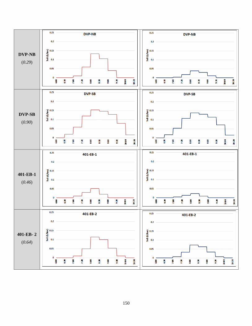
150

DVP-NB

(0.29)

DVP-SB

(0.90)

401-EB-1

(0.46)

401-EB- 2

(0.64)

151

401-WB-2

(0.77)

401-WB-3

(0.75)

7.3.2. Comparative Assessment of Network Performance under Tolling Scenario II

in Different Cases

This section provides a comprehensive comparative assessment involving travel time savings,

monetary savings, overall toll revenues, and system net benefits, for the second tolling scenario

under different situations: base-case, initial toll structures, and fine-tuned toll structures. The

section concludes with a simple cost-benefit analysis provided to investigate the implementation

feasibility of the variable tolling strategies determined via the proposed optimal congestion

pricing system.

7.3.2.1. Network-Wide and Trip-Based Analysis

Table 7-5 summarizes the overall time and monetary savings achieved at different levels along

with the total toll paid (i.e., toll revenues) under the initial and fine-tuned toll structures. The

analysis considers trips at different levels: the entire network, tolled corridors, and tolled routes.

Tolled corridors involve tolled routes and their parallel arterials, as highlighted before. The

152

savings reported in the table, as well as their associated percentages, are calculated relative to the

corresponding base-case values. The monetary values of travel time savings are calculated by

multiplying the corresponding time savings (in hours) by the average VOT used in the GTA

model (15 $/hr.). It should be emphasized that the values presented in the table correspond to the

6:00 to 10:30 am morning period considered here. Moreover, the toll-related statistics illustrated

in the table – namely, the total tolled kilometres travelled and the total toll revenue – are related

only to the tolled routes of the scenario under analysis. That is, the 407 ETR simulated toll

measurements are not included in those statistics, in order to focus on the congestion

management-driven tolling policies that are tested and compared (as opposed to toll revenue-

maximizing approaches that price out more users and may leave parts of the network

underutilized).

The toll levels of the fine-tuned (i.e. optimized) toll structures are generally lower than those of

the initial toll structures, as can be observed from Table 7-4. As a result, the total toll revenues

collected in the former case are lower than in the latter case, as noted in

Table 7-5. Additionally, the ‘tolled kilometres travelled’ under fine-tuned tolls are higher than

those travelled under initial tolls. The travel time savings achieved – at all levels – under fine-

tuned tolls are higher than those achieved under initial tolls. This improvement in travel times

was expected to occur as a result of the initial toll fine-tuning (optimization) process. An overall

cost-benefit analysis is provided at the end of this section for the two key stakeholders: the toll-

system provider (e.g., the government) and the toll payers.

The percentage of relative travel time savings – highlighted in Table 7-5 – decreases across the

three trip-levels considered, i.e. tolled routes’ users, tolled corridors’ users, and all network

users, respectively. This is attributed to the fact that travel time savings resulting from tolling

certain (limited) network routes become more diluted the larger the scale of the population

among which savings are measured. However, the fact that travel times improved at higher trip-

levels, even marginally, indicate that the toll strategies imposed did not exacerbate the traffic

conditions on other non-tolled routes or areas, which is important. This is because any tolling,

optimized or not, will improve the tolled facility performance, but possibly at the expense of

parallel arterials or other parts of the network. Optimized tolling, however, improves the system

at all levels.

153

Table 7-5: Overall Savings against Toll Paid in Different Cases

During (6:00 to 10:30)

Morning Period

Initial (Sub-Optimal) Toll

Structures

Fine-Tuned (Optimized)

Toll Structures

Network-Wide (2 million trips)

Total Travel Time Savings 4327 hr. (0.7%) 10,313 hr. (1.7%)

Monetary Value of Total

Travel Time Savings $64,905 $154,695

Total Tolled Kilometres

Travelled 1,748,081 km 1,837,013 km

Total Toll Revenue $174,829 $147,750

Trips Using Tolled Corridors (455,000 trips)

Total Travel Time Savings 7719 hr. (2.87%) 7831 hr. (2.91%)

Monetary Value of Total

Travel Time Savings $115,783 $117,467

Monetary Value of Total

Schedule-Delay Savings $27,518 $21,540

Trips Using Tolled Routes (220,000 trips)

Total Travel Time Savings 11,712 hr. (7%)

for 219919 toll payers

12,457 hr. (7.5%)

for 220925 toll payers

Monetary Value of Total

Travel Time Savings $175,678 $186,854

Monetary Value of Total

Schedule-Delay Savings $57,047 $50,798

Furthermore, the absolute travel time savings achieved network-wide are lower than those

achieved by toll payers (i.e., tolled routes’ users) in both cases, as is clear in the table. This is

probably due to the increased travel times on routes and time-intervals affected by route-shift and

departure time shift impacts of variable tolling, respectively. It should be emphasized, however,

154

that the spatial and temporal traffic re-distribution (prompted by variable tolling) that results in

alleviated congestion on over-utilized routes and time intervals and increased flow (hence travel

time) levels on under-utilized routes and time intervals, is desirable from a network performance

perspective, as long as the resulting increased inflow values are below capacity. The efficiency

of the spatial and temporal traffic distribution – resulting from variable tolling – is evaluated

through the utilization levels of affected routes and time intervals, as will be demonstrated in the

tolled corridors analysis results.

It can also be seen from Table 7-5 that the difference between the absolute travel time savings of

‘toll payers’ and ‘network-wide users’ is clearly smaller under fine-tuned tolls compared to the

initial-tolls. This is due to the improved utilization levels of parallel arterials (affected by route

shifts) achieved under the fine-tuned toll structures, as will be demonstrated later in Section

7.3.2.2.

Although there was a concern that the schedule-delay costs would increase after variable tolling

due to departure time shifts to early and late (low-toll) intervals, the statistics reported in

Table 7-5 indicate that schedule-delay costs decreased under both tolling structures. Moreover,

the fine-tuned tolls resulted in lower schedule-delay savings than the initial tolls. These remarks

will be explained through the observed trip-length and travel time patterns after tolling, presented

next.

Figure 7-4 shows the changes in: (a) departure time choices, (b) pattern of average trip lengths,

and (c) average travel times for the original 455,000 commuting trips that travelled through the

tolled corridors in the morning period, under different tolling cases. This analysis involves all

trips affected by tolling, including those passing through the tolled routes, those diverting from

the tolled routes to other alternative routes after tolling, and those on the parallel arterials that

might be affected by route shifts out of the tolled routes.

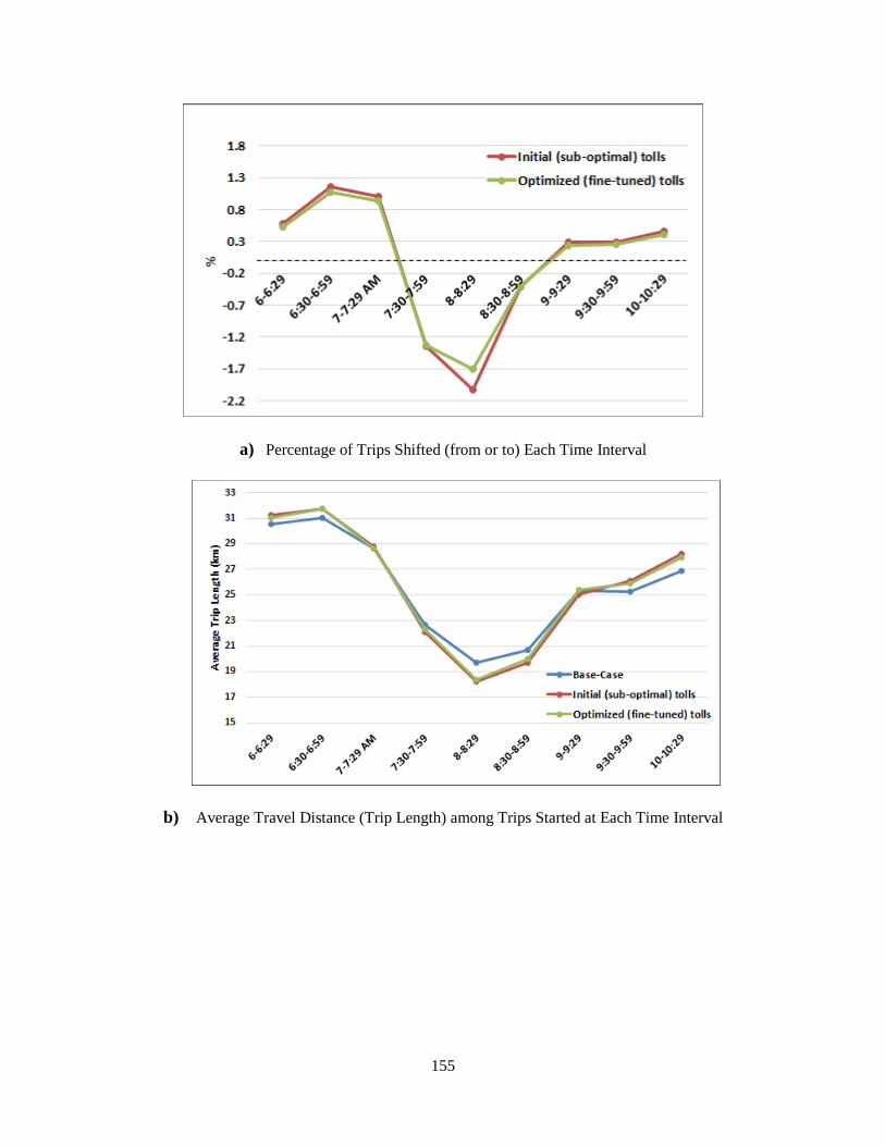
155

a) Percentage of Trips Shifted (from or to) Each Time Interval

b) Average Travel Distance (Trip Length) among Trips Started at Each Time Interval

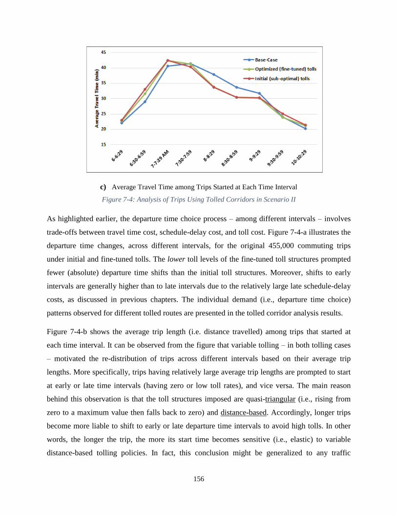
156

c) Average Travel Time among Trips Started at Each Time Interval

Figure 7-4: Analysis of Trips Using Tolled Corridors in Scenario II

As highlighted earlier, the departure time choice process – among different intervals – involves

trade-offs between travel time cost, schedule-delay cost, and toll cost. Figure 7-4-a illustrates the

departure time changes, across different intervals, for the original 455,000 commuting trips

under initial and fine-tuned tolls. The lower toll levels of the fine-tuned toll structures prompted

fewer (absolute) departure time shifts than the initial toll structures. Moreover, shifts to early

intervals are generally higher than to late intervals due to the relatively large late schedule-delay

costs, as discussed in previous chapters. The individual demand (i.e., departure time choice)

patterns observed for different tolled routes are presented in the tolled corridor analysis results.

Figure 7-4-b shows the average trip length (i.e. distance travelled) among trips that started at

each time interval. It can be observed from the figure that variable tolling – in both tolling cases

– motivated the re-distribution of trips across different intervals based on their average trip

lengths. More specifically, trips having relatively large average trip lengths are prompted to start

at early or late time intervals (having zero or low toll rates), and vice versa. The main reason

behind this observation is that the toll structures imposed are quasi-triangular (i.e., rising from

zero to a maximum value then falls back to zero) and distance-based. Accordingly, longer trips

become more liable to shift to early or late departure time intervals to avoid high tolls. In other

words, the longer the trip, the more its start time becomes sensitive (i.e., elastic) to variable

distance-based tolling policies. In fact, this conclusion might be generalized to any traffic

157

policies affecting travel times or costs. i.e., travel behavioural choices (e.g., mode, route, and/or

departure time) of long trips are generally expected to be more elastic to variable traffic policies.

This is due to the fact that these trips suffer more from increased travel times or toll levels.

Figure 7-4-c illustrates the average travel time values of trips that started at different intervals in

the base-case and under ‘initial’ and ‘fine-tuned’ tolls. The average travel times observed at early

and late intervals after tolling (in both cases) are higher than those observed in the base-case.

This is mostly attributed to the longer average lengths of trips that started during those intervals

(Figure 7-4-b), which obviously entails longer average trip times. The net travel time savings

obtained in both tolling cases, relative to the base-case, are reported in

Table 7-5 under the tolled corridor users’ statistics.

The trip-length distribution patterns observed after tolling, the heterogeneity considered in

travellers’ attributes and desired arrival times, along with the improved travel times during peak

hours, are probably the main reasons behind the schedule-delay savings attained after tolling (

Table 7-5). More specifically, longer trips lend themselves to starting at earlier intervals, as a

result of tolling, incurring lower congestion (hence travel time) levels, and hence arriving at their

destinations at earlier times (that are probably closer to their desired arrival times) compared to

their base-case arrival times. On the other hand, trips that started during peak (middle) intervals

after tolling incur fewer queueing-delays than the base-case, and hence arrive at their

destinations at times closer to their desired arrival times as well. It can therefore be concluded

that variable distance-based tolling might result in lower overall schedule-delay costs (compared

to the base-case) when travellers have diverse trip lengths and heterogeneous attributes and

desired arrival times, which is the case in large urban networks. In fact, this observation agrees

with the findings of Newell (1987), which indicate that additional gains may arise when users are

heterogeneous due to arrival time adjustments, which do not occur with homogeneous users. In

particular, that study concluded that the optimum time-varying tolls in a bottleneck reduced the

aggregate schedule-delay costs of two groups of travellers (of equal size) having identical

desired arrival times, but different relative costs of schedule-delay versus travel delay. From

another perspective, the schedule-delay savings achieved under fine-tuned tolls are lower than

those achieved under initial tolls, as observed in

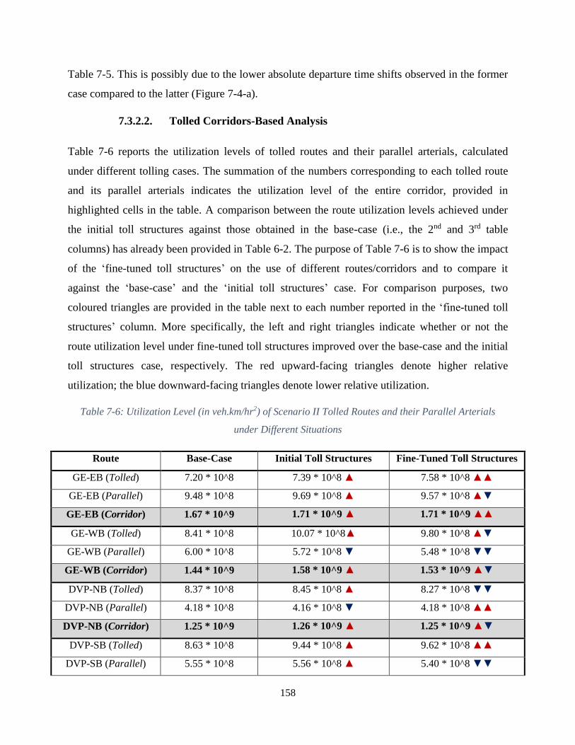
158

Table 7-5. This is possibly due to the lower absolute departure time shifts observed in the former

case compared to the latter (Figure 7-4-a).

7.3.2.2. Tolled Corridors-Based Analysis

Table 7-6 reports the utilization levels of tolled routes and their parallel arterials, calculated

under different tolling cases. The summation of the numbers corresponding to each tolled route

and its parallel arterials indicates the utilization level of the entire corridor, provided in

highlighted cells in the table. A comparison between the route utilization levels achieved under

the initial toll structures against those obtained in the base-case (i.e., the 2nd and 3rd table

columns) has already been provided in Table 6-2. The purpose of Table 7-6 is to show the impact

of the ‘fine-tuned toll structures’ on the use of different routes/corridors and to compare it

against the ‘base-case’ and the ‘initial toll structures’ case. For comparison purposes, two

coloured triangles are provided in the table next to each number reported in the ‘fine-tuned toll

structures’ column. More specifically, the left and right triangles indicate whether or not the

route utilization level under fine-tuned toll structures improved over the base-case and the initial

toll structures case, respectively. The red upward-facing triangles denote higher relative

utilization; the blue downward-facing triangles denote lower relative utilization.

Table 7-6: Utilization Level (in veh.km/hr2) of Scenario II Tolled Routes and their Parallel Arterials

under Different Situations

Route Base-Case Initial Toll Structures Fine-Tuned Toll Structures

GE-EB (Tolled) 7.20 * 10^8 7.39 * 10^8 ▲ 7.58 * 10^8 ▲▲

GE-EB (Parallel) 9.48 * 10^8 9.69 * 10^8 ▲ 9.57 * 10^8 ▲▼

GE-EB (Corridor) 1.67 * 10^9 1.71 * 10^9 ▲ 1.71 * 10^9 ▲▲

GE-WB (Tolled) 8.41 * 10^8 10.07 * 10^8▲ 9.80 * 10^8 ▲▼

GE-WB (Parallel) 6.00 * 10^8 5.72 * 10^8 ▼ 5.48 * 10^8 ▼▼

GE-WB (Corridor) 1.44 * 10^9 1.58 * 10^9 ▲ 1.53 * 10^9 ▲▼

DVP-NB (Tolled) 8.37 * 10^8 8.45 * 10^8 ▲ 8.27 * 10^8 ▼▼

DVP-NB (Parallel) 4.18 * 10^8 4.16 * 10^8 ▼ 4.18 * 10^8 ▲▲

DVP-NB (Corridor) 1.25 * 10^9 1.26 * 10^9 ▲ 1.25 * 10^9 ▲▼

DVP-SB (Tolled) 8.63 * 10^8 9.44 * 10^8 ▲ 9.62 * 10^8 ▲▲

DVP-SB (Parallel) 5.55 * 10^8 5.56 * 10^8 ▲ 5.40 * 10^8 ▼▼

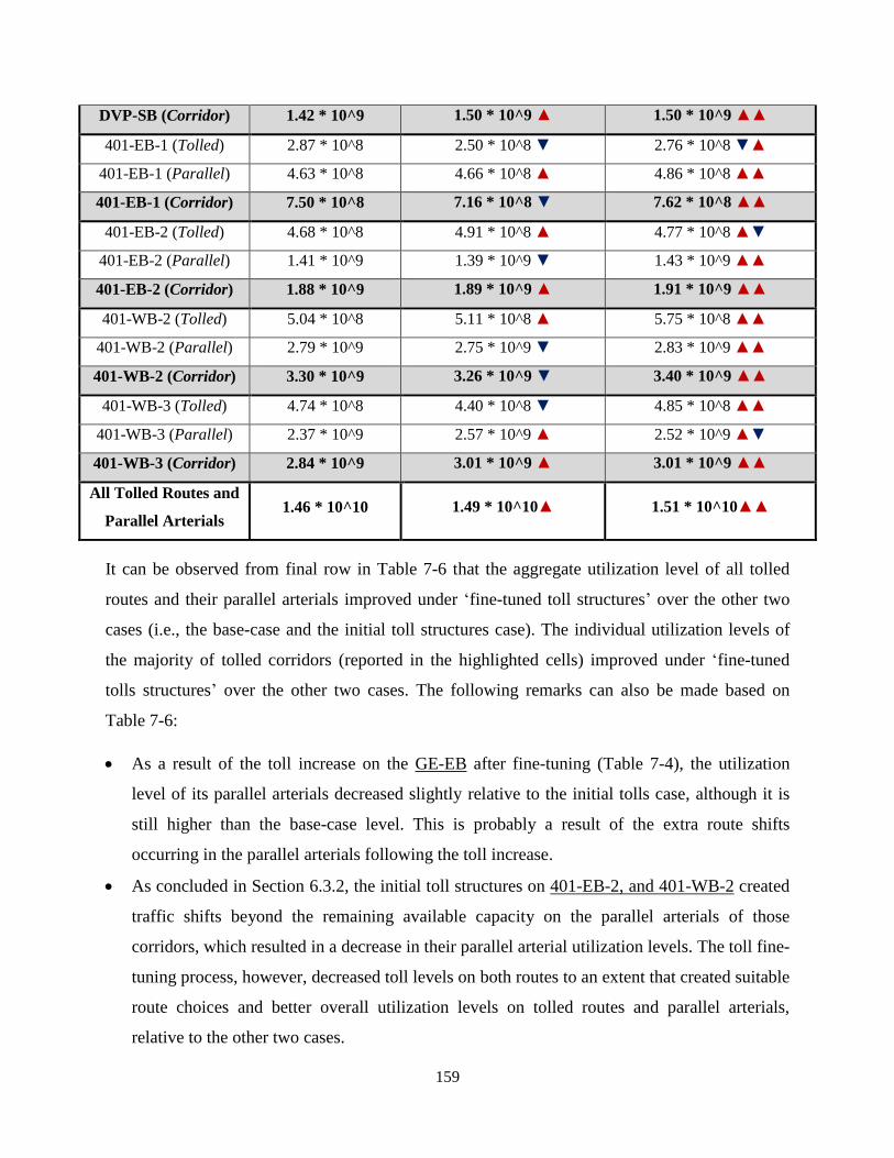
159

DVP-SB (Corridor) 1.42 * 10^9 1.50 * 10^9 ▲ 1.50 * 10^9 ▲▲

401-EB-1 (Tolled) 2.87 * 10^8 2.50 * 10^8 ▼ 2.76 * 10^8 ▼▲

401-EB-1 (Parallel) 4.63 * 10^8 4.66 * 10^8 ▲ 4.86 * 10^8 ▲▲

401-EB-1 (Corridor) 7.50 * 10^8 7.16 * 10^8 ▼ 7.62 * 10^8 ▲▲

401-EB-2 (Tolled) 4.68 * 10^8 4.91 * 10^8 ▲ 4.77 * 10^8 ▲▼

401-EB-2 (Parallel) 1.41 * 10^9 1.39 * 10^9 ▼ 1.43 * 10^9 ▲▲

401-EB-2 (Corridor) 1.88 * 10^9 1.89 * 10^9 ▲ 1.91 * 10^9 ▲▲

401-WB-2 (Tolled) 5.04 * 10^8 5.11 * 10^8 ▲ 5.75 * 10^8 ▲▲

401-WB-2 (Parallel) 2.79 * 10^9 2.75 * 10^9 ▼ 2.83 * 10^9 ▲▲

401-WB-2 (Corridor) 3.30 * 10^9 3.26 * 10^9 ▼ 3.40 * 10^9 ▲▲

401-WB-3 (Tolled) 4.74 * 10^8 4.40 * 10^8 ▼ 4.85 * 10^8 ▲▲

401-WB-3 (Parallel) 2.37 * 10^9 2.57 * 10^9 ▲ 2.52 * 10^9 ▲▼

401-WB-3 (Corridor) 2.84 * 10^9 3.01 * 10^9 ▲ 3.01 * 10^9 ▲▲

All Tolled Routes and

Parallel Arterials 1.46 * 10^10 1.49 * 10^10▲ 1.51 * 10^10▲▲

It can be observed from final row in Table 7-6 that the aggregate utilization level of all tolled

routes and their parallel arterials improved under ‘fine-tuned toll structures’ over the other two

cases (i.e., the base-case and the initial toll structures case). The individual utilization levels of

the majority of tolled corridors (reported in the highlighted cells) improved under ‘fine-tuned

tolls structures’ over the other two cases. The following remarks can also be made based on

Table 7-6:

As a result of the toll increase on the GE-EB after fine-tuning (Table 7-4), the utilization

level of its parallel arterials decreased slightly relative to the initial tolls case, although it is

still higher than the base-case level. This is probably a result of the extra route shifts

occurring in the parallel arterials following the toll increase.

As concluded in Section 6.3.2, the initial toll structures on 401-EB-2, and 401-WB-2 created

traffic shifts beyond the remaining available capacity on the parallel arterials of those

corridors, which resulted in a decrease in their parallel arterial utilization levels. The toll fine-

tuning process, however, decreased toll levels on both routes to an extent that created suitable

route choices and better overall utilization levels on tolled routes and parallel arterials,

relative to the other two cases.

160

As concluded in Section 6.3.2, the initial toll structures on 401-WB-3 and 401-EB-1 resulted

in an underutilization of tolled routes and better utilization of parallel arterials, probably due

to their readily available capacity that absorbed the traffic that shifted in response to tolling.

It can be noticed from Table 7-6 that this problem was tackled through the lower fine-tuned

toll structures on both routes, which produced better utilization levels.

It can also be observed that slight toll decreases on 401-EB-1 (3 ¢/km) and 401-WB-2 (5

¢/km), following the initial toll structures fine-tuning process, resulted in obvious

improvements in the utilization levels of both routes and their parallel arterials. This confirms

the conclusion made earlier regarding the various sensitivity levels of different tolled routes

to identical toll changes, which further emphasizes the significance of the toll fine-tuning

process and the route-based analysis conducted.

The observed changes in route utilization levels in response to fine-tuned toll structures are

further explained/interpreted through the tolled-routes detailed analysis presented next.

Table 7-7 presents illustrative diagrams in which the demand and travel time patterns on tolled

routes are compared across different tolling cases. In particular, each figure provided in the

‘departure time choice’ column illustrates the demand pattern (i.e., the number of trips generated

at different time-intervals) of the associated tolled route in the base-case and under fine-tuned

toll structures. Moreover, the percentage decrease in the number of trips using the tolled routes

(under fine-tuned tolls) is highlighted on the top part of each figure. The percentages are

calculated for each tolled route – over all the morning period, tolled period, and non-tolled

period – relative to the base-case demand generated during each period. The negative

percentages obtained at some periods denote a relative increase in the tolled route demand during

those periods compared to the base-case. The demand patterns and percentage decreases

provided in the table articulate the route and departure time shift impacts of the fine-tuned toll

structures on the demand of tolled routes at different periods.

The figures provided in the right-hand column of Table 7-7 give the estimated travel time

patterns on tolled routes in the base-case, under initial toll structures, and under fine-tuned toll

structures. The routes’ travel time values at capacity are also highlighted in the figures (through

the straight purple lines). As described before, the vertical gap between the travel time pattern

and the travel time at capacity (when the former surpasses the latter) represents the queueing-

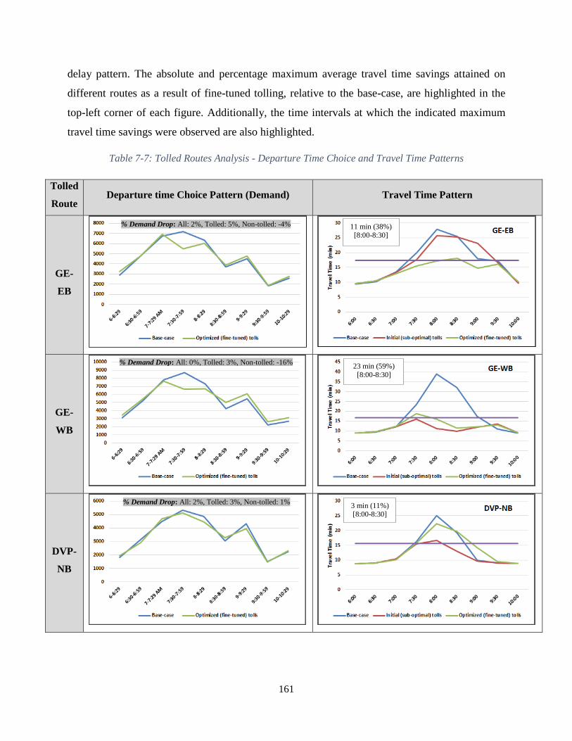
161

delay pattern. The absolute and percentage maximum average travel time savings attained on

different routes as a result of fine-tuned tolling, relative to the base-case, are highlighted in the

top-left corner of each figure. Additionally, the time intervals at which the indicated maximum

travel time savings were observed are also highlighted.

Table 7-7: Tolled Routes Analysis - Departure Time Choice and Travel Time Patterns

Tolled

Route Departure time Choice Pattern (Demand) Travel Time Pattern

GE-

EB

GE-

WB

DVP-

NB

3 min (11%) [8:00-8:30]

% Demand Drop: All: 2%, Tolled: 3%, Non-tolled: 1%

23 min (59%)

[8:00-8:30]

% Demand Drop: All: 0%, Tolled: 3%, Non-tolled: -16%

11 min (38%)

[8:00-8:30]

% Demand Drop: All: 2%, Tolled: 5%, Non-tolled: -4%

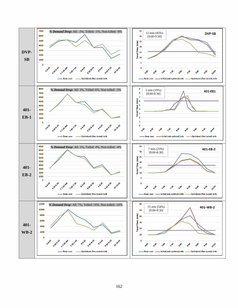
162

DVP-

SB

401-

EB-1

401-

EB-2

401-

WB-2

15 min (54%) [9:00-9:30]

% Demand Drop: All: 7%, Tolled: 16%, Non-tolled: -16%

7 min (23%) [8:00-8:30]

% Demand Drop: All: 2%, Tolled: 4%, Non-tolled: -4%

2 min (19%) [8:00-8:30]

% Demand Drop: All: 3%, Tolled: 6%, Non-tolled: -3%

12 min (45%)

[9:00-9:30]

% Demand Drop: All: -2%, Tolled: -1%, Non-tolled: -9%

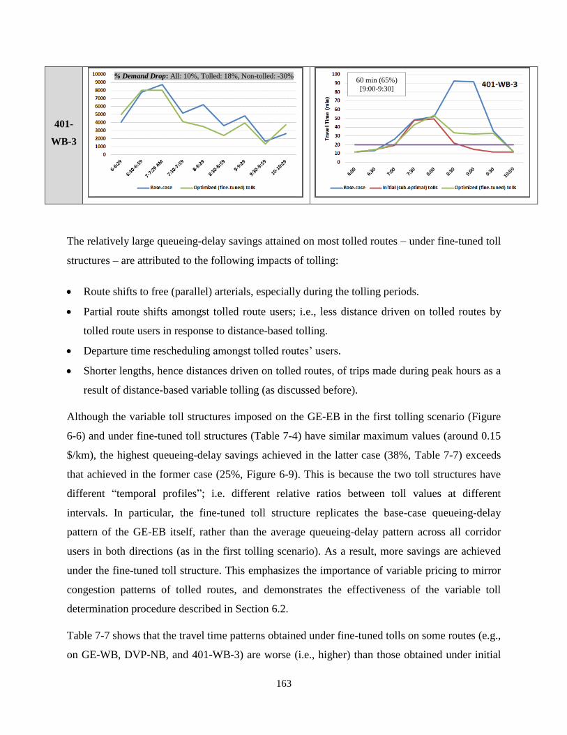
163

401-

WB-3

The relatively large queueing-delay savings attained on most tolled routes – under fine-tuned toll

structures – are attributed to the following impacts of tolling:

Route shifts to free (parallel) arterials, especially during the tolling periods.

Partial route shifts amongst tolled route users; i.e., less distance driven on tolled routes by

tolled route users in response to distance-based tolling.

Departure time rescheduling amongst tolled routes’ users.

Shorter lengths, hence distances driven on tolled routes, of trips made during peak hours as a

result of distance-based variable tolling (as discussed before).

Although the variable toll structures imposed on the GE-EB in the first tolling scenario (Figure

6-6) and under fine-tuned toll structures (Table 7-4) have similar maximum values (around 0.15

$/km), the highest queueing-delay savings achieved in the latter case (38%, Table 7-7) exceeds

that achieved in the former case (25%, Figure 6-9). This is because the two toll structures have

different “temporal profiles”; i.e. different relative ratios between toll values at different

intervals. In particular, the fine-tuned toll structure replicates the base-case queueing-delay

pattern of the GE-EB itself, rather than the average queueing-delay pattern across all corridor

users in both directions (as in the first tolling scenario). As a result, more savings are achieved

under the fine-tuned toll structure. This emphasizes the importance of variable pricing to mirror

congestion patterns of tolled routes, and demonstrates the effectiveness of the variable toll

determination procedure described in Section 6.2.

Table 7-7 shows that the travel time patterns obtained under fine-tuned tolls on some routes (e.g.,

on GE-WB, DVP-NB, and 401-WB-3) are worse (i.e., higher) than those obtained under initial

60 min (65%)

[9:00-9:30]

% Demand Drop: All: 10%, Tolled: 18%, Non-tolled: -30%

164

toll structures. This is because the objective of the toll fine-tuning process performed was to

adjust toll levels in order to maintain proper utilization levels on tolled routes and their parallel

arterials. In other words, decreased travel times on tolled routes associated with deteriorated

traffic conditions on parallel arterials (e.g., parallel arterials of DVP-NB under initial tolls) or

underutilized tolled route capacity (e.g. GE-WB under initial tolls) are not desired.

Interestingly, the two figures corresponding to the DVP-SB (in Table 7-7) indicate that the travel

time pattern on that route clearly improved under fine-tuned tolls, despite the fact that its total

demand slightly increased after tolling. This is most probably a result of the departure time shifts

observed on that route in response to variable tolling. This observation demonstrates the benefits

achieved from proper departure time rescheduling under similar (or even higher) numbers of

route users.

7.3.2.3. Cost-Benefit Analysis of Optimal Toll Strategies

In order to appraise the implementation feasibility of the tolling strategies determined by the

optimal congestion pricing system, an annual cost-benefit analysis is conducted for the two key

stakeholders: the producer (e.g. the government) and the consumers (toll payers). The producer,

in this context, refers to the entity that incurs the toll-system implementation and operations costs

– for the sake of traffic congestion management – and collects the toll revenues. The consumers

are the actual toll-system users who care about obtaining benefits in response to the toll paid; i.e.,

the consumers are the toll payers.

As indicated in Table 7-8, the overall costs from a producer’s perspective involve the capital cost

(incurred once) associated with the initial toll-system implementation, in addition to the annual

maintenance and operations costs. On the other hand, the overall producer benefits consist of the

monetary value of the network-wide travel time savings as a result of tolling, as well as the toll

revenues collected. Travel time savings are included as a producer benefit, since it is assumed to

be the main objective sought by the government via congestion pricing (as a traffic management

tool), as opposed to revenue maximizing (monopoly) pricing approaches. On the other hand, the

cost incurred by consumers is the total amount of toll paid; their benefits include the monetary

value of their own travel time and schedule-delay savings as a result of tolling. Schedule-delay

165

changes are assumed only to concern toll payers; therefore, they are not considered in the overall

producer benefits, as they do not explicitly affect the traffic network performance.

Table 7-8: Annual Cost-Benefit Analysis (under Optimized Tolls) from the Perspectives of the Producer

and Consumer

Entity Overall Costs

($ Millions)

Overall Benefits

($ Millions)

Benefit-Cost

Ratio

Government

(Producer)

Capital

Implementation

Cost:

Annual

Operations

Cost:

Toll

Revenues

Travel Time

Savings

2.15

(after 1st year) 88.5 73.2 76.8 80.5

Total Producer Costs:

1st year: 161.7

After 1st year: 73.2

Total Producer Benefits:

157.3

Toll Payers

(Consumers)

Toll Paid:

76.8

Travel Time

Savings

Schedule-

Delay

Savings 1.61

97.2 26.4

Total Consumer Benefits:

123.6

The annual values reported in Table 7-8 for the total toll collected, the monetary value of travel

time savings network-wide, and the monetary value of travel time and schedule-delay savings

across toll payers, were calculated based on the corresponding values reported in

Table 7-5 (under the ‘optimized’ toll structures case). As stressed earlier, the values presented in

the latter table correspond to the 6:00 to 10:30 am morning period. Therefore, two assumptions

were made to estimate the savings/revenues that can be obtained annually under the same

optimal toll strategies. First, it was assumed that the same optimal toll structures will be imposed

in the morning and afternoon periods (i.e., twice a day), during weekdays (i.e., five times a

week), and over the entire year (i.e., 52 weeks). The second assumption is that the same

savings/revenues, reported in

166

Table 7-5, will be attained during each and every (morning or afternoon) tolling period.

According to those assumptions, the annual savings/revenues – reported in Table 7-8 – were

calculated by multiplying the corresponding values in Table 7-5 by (two daily tolling periods *

five weekdays * 52 weeks).

The producer-related costs, presented in Table 7-8, were calculated based on a report conducted

by Lively and Rossini (2015), in which the authors developed estimates for the capital and

operations costs of a distance-based tolling system for the GE and the DVP. The capital costs

estimated in that report include 1) the roadside costs (associated with gantry structures, toll

hardware/software and communication devices at each toll point); and 2) the central control

system costs (associated with the hardware/software to support processing transactions and the

operational centre staff). The estimated annual costs involve 1) the annual maintenance costs for

24/7 maintenance of the toll system hardware and software; 2) the annual replacement/upgrade

fund to perform regular system upgrades; and 3) the annual operational costs for processing toll

transactions, billing customers and providing customer service (Lively and Rossini, 2015). The

total length of the eight tolled routes/segments considered in the second tolling scenario (being

evaluated) is almost double that of the four directions of the GE and the DVP. Therefore, the

toll-system capital and annual costs (given in Table 7-8) were roughly calculated by doubling the

corresponding values estimated in Lively and Rossini (2015) for the GE and DVP toll systems.

As highlighted in Table 7-8, the ‘benefit-to-cost ratio’ from a toll payer’s perspective is 1.61,

which shows that toll payers benefit from tolling even before toll revenues are spent. The ratio

attained is well above the unity ratio obtained in the Bottleneck Model, in which the toll replaces

queueing-delay dollar-for-dollar as a means of rationing road space. This could be attributed to

the following factors: 1) the schedule-delay savings obtained under fine-tuned tolls, which

represent around 30% of consumers’ costs; 2) the extra travel time savings achieved on tolled

routes due to route shifts to parallel arterials; and 3) the decreased toll values (i.e., cost) on most

tolled routes, after fine-tuning, compared to the initial ‘Bottleneck’ toll values disregarding the

effect of tolling on parallel arterials. The ‘benefit-to-cost ratio’ from a producer’s perspective is

2.15. It can also be inferred from the table statistics that the producer’s net benefits attained in

the first year represent more than 95% of the capital implementation cost. These findings clearly

indicate that the tolling policies determined through the optimal congestion pricing system –

167

proposed here – offer a win-win solution in which travel times and overall network performance

are improved, while raising funds to invest in sustainable transportation infrastructure, which is

desirable from both the public and the government perspectives.

7.3.3. Final Remarks and Conclusions

This chapter has presented the design and implementation details of the “Optimal Toll

Determination – Level II” module, which concludes the full optimal congestion pricing system

implementation. The details provided in this chapter have demonstrated: 1) the efforts exerted to

tackle the objective function-related issues through a problem-segmentation methodological

approach; 2) the challenges associated with integrating and configuring a middleware (to the GA

platform) for distributed computations on a parallel cluster; and 3) the effectiveness and

implementation feasibility of the tolling strategies determined through the optimal congestion

pricing system for a case study in the GTA region. The results and analysis presented

demonstrate the benefits achieved, at different levels, under the determined optimal tolling

strategies. The benefits come from the route and departure time shift impacts of distance-based

variable tolling.

In fact, the determination of proper pricing strategies to manage traffic demand and congestion is

challenging in large-scale interconnected congested networks (like the GTA). In the special case

of tolling specific congested routes in the network, improperly high toll levels might excessively

send traffic to off-ramps to parallel arterials, which can generate counterproductive results. On

the other hand, moderate toll levels intended to maintain adequate utilization levels of tolled

routes and their parallel arterials might not induce the expected rescheduling benefits of variable

tolling. In other words, the desired behavioural changes in route and departure time choices

might be contradictory in some situations. Accordingly, variable tolling strategies intended to

manage traffic congestion – by distributing demand more evenly over time and space – should be

carefully crafted while considering 1) the criticality/sensitivity of the tolled routes, 2) the traffic

conditions and available capacity on parallel arterials, and 3) the entire traffic network

interconnectivity.

The optimal congestion pricing system developed here provides a new and comprehensive tool

for optimal tolling strategy determination and evaluation in large-scale networks. The system’s

168

robustness and effectiveness have been examined through simulation-based case studies in the

GTA region. The results demonstrate that properly constructed and optimized variable tolling

policies result in moderate route and departure time shifts that bring obvious traffic benefits. In

conclusion, the tolling policies determined through the optimal congestion pricing tool offer a

win-win solution in which travel times and overall network performance are improved, while

also raising funds to invest in sustainable transportation infrastructure.

169

8. Conclusions

Congestion pricing is widely viewed among economists and practitioners as one of the most

promising control tools to tackle traffic congestion. A significant body of research has been

conducted thus far in this area. However, theoretically and/or methodologically sound studies are

often applied to small or even hypothetical networks, i.e. case studies on large-scale urban

network models are scarce. Additionally, the tolling scenarios applied in most practically

oriented studies lack methodological justification. Furthermore, the users’ individual responses

to pricing (e.g. departure time and route choices) are usually disregarded; if considered, the

impact of personal and socio-economic attributes on their choices was often not captured.

This dissertation has focused on developing a system for optimal congestion pricing policy

determination and evaluation to manage peak period travel demand, while explicitly capturing

departure time and route choices in a large-scale DTA simulation environment. The system seeks

the congestion pricing policies that achieve the best spatial and temporal traffic distribution and

infrastructure utilization to optimize the network performance (i.e., minimize the total travel

times).

The system involves a departure time choice model extended to incorporate tolls and schedule-

delay cost components – in addition to driver- and trip-related attributes – for comprehensive

modelling of the morning peak travel behaviour. Through the extensive travel survey data

available in the GTA, we have considered the heterogeneity in drivers’ values of (early or late)

schedule-delay and desired arrival time. The optimal congestion pricing policies are obtained

through a bi-level procedure. The first level involves determining variable queue-eliminating toll

structures for congested facilities motivated by the Bottleneck Model of dynamic congestion

pricing. The second level involves iterative optimization fine-tuning of the toll structures

determined in the first level to achieve the best possible network performance while considering

the route and departure time shift impacts of tolling network-wide. The second level uses a

robust iterative optimization algorithm that is run concurrently (i.e., distributed) on a parallel

computing cluster.

170

The time-dependent tolling scheme adopted in the congestion pricing system is also distance-

based: each vehicle pays according to the distance travelled on tolled facilities. This tolling

scheme aims to attain spatial equity besides diminishing the incentives for drivers to slow down

or stop before specific toll-collection locations. Additionally, it creates an incentive for drivers to

minimize the distances driven on the tolled routes; a type of behaviour denoted here as ‘partial

route-shift’.

Concisely, the developed optimal congestion pricing system consists of the following four main

modules:

1. A large-scale calibrated DTA simulation platform, covering most of the GTA region, which

is used to assess the impact of various pricing options on routing and congestion patterns;

2. An econometric (behavioural) model of departure time choice that is built and calibrated

using regional household travel survey data, capturing the heterogeneity of travellers’

personal and socio-economic attributes;

3. The Bottleneck Model for dynamic congestion pricing, which is the theoretical basis of the

initial variable toll structures determination approach adapted here; and

4. A robust iterative distributed optimization approach for toll structure fine-tuning to achieve

the best possible network performance.

All these modules are integrated and implemented into a single system that incorporates iterative

optimization of variable tolling while looping between the departure time choice layer and the

DTA layer until departure time choices and route choices reach equilibrium, under each tolling

scenario being assessed during optimization. For the system’s large-scale nature and the

consequent (time and memory) computational challenges, the optimization algorithm is run

concurrently on a parallel computing cluster.

The system is intended to be general and applicable to a variety of tolling scenarios (e.g.

congested highway sections, HOT lanes, and cordon tolls). As a first implementation, it was used

to determine and evaluate optimal distance-based variable tolling strategies for key congested

freeways in the GTA region. The impacts were assessed at the regional level, trip level, and the

tolled-corridor level. Moreover, a cost-benefit analysis was conducted for the two key

171

stakeholders, i.e. the producer (e.g. the government) and the consumers (toll payers). The results

confirm the robustness and effectiveness of the proposed optimal congestion pricing system.

8.1. Summary

Chapter 1 of the dissertation started with a description of the motivation behind this research

effort. It also highlighted the limitations of existing congestion pricing studies and outlined the

research objectives. The chapter concluded with a high-level description of the proposed optimal

congestion pricing system.

Chapter 2 provided an overview of the main economic models of congestion pricing, along with

their objectives and implications. A literature review of the state-of-art and the state-of-practice

of congestion pricing was also provided. The chapter concluded with a summary of the

gaps/limitations in the dynamic congestion pricing models developed/implemented that

motivated this research.

Chapter 3 presented a brief overview of the full optimal congestion pricing system, including the

four main modules along with their integration and iteration. The chapter also highlighted the

different input data types provided to the system, i.e. simulation testbed-related data and tolling

scenario-related data.

Chapter 4 described the process followed to build, calibrate, and validate a large-scale DTA

simulation model (covering most of the GTA region) based on the most recently available TTS

demand data, GTA TAZs system, network geometry information, and loop-detector feeds. The

chapter concluded with a discussion of the challenges associated with that model.

Chapter 5 described the details of the departure time choice model integrated to the optimal

congestion pricing system, including the choice set formulation and the original model variables.

The chapter then discussed the extensions carried out to incorporate schedule-delay and toll cost

components in the model, and to re-calibrate the associated parameters. The

preparation/estimation details of the data required by the model were also presented. The

implementation details, the convergence criterion, and the model base-case validation results

were then illustrated. The chapter concluded with a summary of the challenges associated with

retrofitting and implementing the departure time choice model.

172

Chapter 6 presented the details of the first level of optimal toll determination in the congestion

pricing system. The chapter started with an overview of the adopted theoretical economic model

for dynamic congestion pricing, i.e. the Bottleneck Model. After that, the procedure followed to

identify the congested facilities to be tolled and to calculate their initial toll structures motivated

by the Bottleneck Model was described. The procedure was then applied and tested on two

tolling scenarios of major highways in the GTA. The chapter concluded with a general

discussion and insights driven from the preliminary results of the tested partially optimized

tolling scenarios.

Chapter 7 described the second level of optimal toll determination in the congestion pricing

system. The chapter started with a description of the different optimization problem components

and the procedure followed to tackle some objective function-related issues. An overview was

then given of the GA used for optimization and the choice of its parameters. After that, the

middleware integrated into the optimization platform for distributed computing was described,

along with the configuration process conducted for the parallel cluster used. The chapter then

presented the implementation details of the optimization module on the extended tolling scenario

considered for the GTA (introduced in Chapter 6), after which a comprehensive comparative

assessment was provided for the same scenario under different situations. The chapter concluded

with a cost-benefit analysis provided to investigate the implementation feasibility of the tolling

strategies determined via the proposed optimal congestion pricing system.

8.2. Major Findings

The analysis of the flat and variable tolling structures presented in the first GTA tolling scenario

(Gardiner Expressway) in Chapter 6 led to the following principal findings:

– In a large-scale interconnected network (like the GTA) where long-distance trips have

diverse routing options, tolling a relatively short, yet major, highway like the GE creates

temporal and spatial traffic changes network-wide that go beyond the tolling interval and the

tolled route. This confirms the importance of conducting the simulations on a regional scale

for policy determination and assessment.

– More benefits are gained from departure time re-scheduling due to variable pricing,

compared to just re-routing as in flat tolling. This emphasizes the importance of the

173

integrated departure time module to the proposed congestion pricing system, to provide

realistic modelling of users' individual departure time responses to variable pricing policies.

– Pricing that only induces re-routing (and no departure time re-scheduling), or excessive re-

routing due to, for instance, overpricing, can send excess traffic to off-ramps to parallel

routes that blocks the off-ramp and backs up onto the main freeway, limiting access to the

priced road itself. This is not only counterproductive, but also nullifies the very purpose of

pricing. This emphasizes the importance of variable pricing to mirror congestion patterns

over time, which is the methodological basis (adapted from the Bottleneck Model) of the

proposed variable tolling framework.

– Less congested (early and late) intervals can realistically attract traffic as a consequence of

variable tolling during the peak period. In other words, the departure time choice process –

among different intervals – involves trade-offs between travel time cost, schedule-delay cost,

and toll cost. Moreover, shifts to early intervals are generally higher than late intervals

because the late arrival shadow price is higher than that of early arrival.

– Congestion pricing on real-world road networks can have different effects to those suggested

by studies of single links or toy networks. For example, unlike in the simple Bottleneck

Model, variable tolling affects not only the cumulative loading curve but also the cumulative

exit curve. Another example is that imposing a flat toll on a link can actually increase travel

time on the link because of spillback.

The analysis of the initial (sub-optimal) toll structures derived for the GTA extended tolling

scenario (eight tolled routes/segments), in Chapter 6, led to the further following conclusions:

– The simple and extended tolling scenarios conducted demonstrated the effectiveness of the

proposed system in 1) determining the initial (sub-optimal) toll structures for congested

facilities, following the Bottleneck Model dynamic pricing rules; 2) simulating the

consequent travellers’ route and departure time choice responses through the integrated

testbed of the departure time and DTA simulation models; and 3) evaluating the network

performance under each scenario.

– The initial toll structures determined via the “first level of optimal toll determination”

module resulted in noticeable overall benefits at different levels. However, further

adjustments are needed for the toll levels of those structures to optimize the utilization of

174

tolled corridors (and hence avoid the undesired impacts of tolling) and minimize the total

travel times, while considering the interconnectivity and interdependency among tolled and

non-tolled facilities in the network.

The detailed analysis conducted in Chapter 6 furnished important information concerning the

choice and design of the optimization variables used via the distributed GA for toll structures

optimization (fine-tuning) in Chapter 7. The optimization algorithm (second level of optimal toll

determination) was applied on the initial toll structures of the GTA extended tolling scenario.

The resulting network performance was compared against those obtained under the initial toll

structures and the base-case. The analysis/comparison conducted in Chapter 7 led to the

following findings:

– In the case of a large number of tolled routes (hence optimization variables), the optimization

algorithm might encounter a quasi-flat objective function issue. i.e., the objective function

takes close values at various solutions tested during optimization, which makes the search

process for the global optimal solution extremely challenging and time-consuming. A

criterion was designed to classify groups of mutually correlated routes and hence optimize

toll structures on each group separately.

– The carefully estimated initial (sub-optimal) toll structures, the concise search spaces

identified for different problems based on the evaluation results of the initial toll structures,

and the relatively large population sizes used, led to relatively fast GA convergence (i.e., low

number of iterations to convergence) considering the large-scale nature of the application.

– Tolled routes have different sensitivity levels to identical toll changes, which emphasizes the

importance of conducting tolled route-based analysis while considering the parallel arterials

and the entire corridor vitality within the network. It also emphasizes the significance of the

toll fine-tuning process

– As a result of the fine-tuned toll structures, the overall travel time savings achieved – at

different levels – are higher than those achieved under initial tolls. Additionally, fine-tuned

tolls avoided the undesired consequences of some initial toll structures, such as underutilized

tolled route or excessive route shifts to parallel arterials. This was demonstrated through the

improved utilization levels of tolled corridors observed under fine-tuned tolls, which reflects

the efficiency of the spatial and temporal traffic distribution resulting from those tolls.

175

– The variable distance-based tolling prompted longer trips to shift to early or late departure

time-intervals to avoid high tolls. i.e., the longer the trip, the more its start time becomes

sensitive (i.e., elastic) to variable distance-based tolling policies. This conclusion could be

generalized to traffic policies affecting travel times or costs. That is, the travel behavioural

choices (e.g., mode, route, and/or departure time) of long trips are expected to be more elastic

to variable traffic policies, due to the fact that those trips suffer more from increased travel

times or toll/fare levels.

– As a consequence of the trip-length redistribution and the improved travel times during peak

hours (resulting from variable distance-based tolling), the overall schedule-delay costs

improved (i.e., decreased) after tolling. Moreover, the schedule-delay savings associated with

the fine-tuned (lower) toll structures are less than those associated with the initial (higher)

toll structures, possibly due to the lower absolute departure time shifts observed under the

former tolls.

– The desired behavioural changes in route and departure time choices might be contradictory

in the case of tolling specific congested routes in a large-scale interconnected network (like

the GTA). High toll levels might excessively send traffic to parallel arterials, which can lead

to counterproductive results. On the other hand, moderate toll levels intended to maintain

adequate utilization levels of tolled routes and their parallel arterials might not induce the

expected rescheduling benefits of variable tolling. Accordingly, variable tolling strategies

intended to manage traffic congestion should be carefully determined depending on the local

conditions of the tolled route and its parallel arterials, while considering the entire traffic

network interconnectivity.

– As a consequence of the previous remark, the optimal toll levels obtained – achieving the

best network performance – are clearly lower than the toll rates of the 407 Express Toll

Route (ETR) in the morning period (average of 0.35 $/km). In other words, congestion

pricing strategies intended to manage traffic demand, rather than to maximize toll revenues,

are carefully crafted to alleviate traffic congestion through proper toll levels and are less

aggressive than revenue-maximizing (monopoly) approaches.

– The cost-benefit analyses conducted for the two key stakeholders indicate that:

o Toll payers benefit from tolling even before toll revenues are spent,

176

o The producer’s net benefits attained in the first year represent more than 95% of the

toll-system capital implementation cost, and

o The producer’s benefit-to-cost ratio exceeds 2.

Therefore, the tolling policies determined through the optimal congestion pricing tool offer a

win-win solution in which travel times and overall network performance are improved, while

also raising funds to invest in sustainable transportation infrastructure.

In conclusion, the queueing-delay savings – hence, restored capacity and improved utilization

levels – resulting from the optimal tolling strategies determined, are attributed to the following

behavioural impacts of tolling:

1. Route shifts to free (parallel) arterials, especially during the tolling periods.

2. Partial route shifts amongst tolled routes’ users; i.e., less distances driven on tolled routes

by tolled routes’ users in response to distance-based tolling.

3. Departure time rescheduling amongst tolled routes’ users.

4. Shorter lengths, hence shorter distances driven on tolled routes, of trips made during peak

hours as a result of distance-based variable tolling.

8.3. Research Contributions

The research presented in this dissertation provides an innovative full-fledged system (tool) for

the optimal time-dependent toll-strategy determination and evaluation in large-scale networks. In

particular, the system carefully determines and evaluates the tolling strategies resulting in the

best spatial and temporal traffic distribution (i.e., route and departure time choices) that works

towards eliminating congestion (queueing-delay) and minimizing the total travel times. In brief,

this study contributes to the state-of-the-art of congestion pricing through the following aspects:

1. Designing a system for optimal congestion pricing determination and evaluation in large-

scale networks.

2. Developing the different system modules for the GTA region. Each module was

implemented by either: a) developing certain component (from scratch) based on the most

recently available GTA data, b) retrofitting exiting models to meet the current research

177

needs, or c) designing a practical procedure that is motivated by an existing theoretical

model.

3. Integrating the large-scale computationally intensive modules developed, which involved

massive communication (i.e., input and output data exchanged) and multiple iterations

performed among different modules.

More specifically, the research presented involves important contributions in many areas, such

as:

1. Developing the optimal congestion pricing system through integrating distinct modules. This

entails two significant characteristics of the system:

a. Any module can be upgraded/replaced separately without the need for rebuilding the full

system. i.e., each module can be altered locally (upon need) without affecting the overall

implemented system structure and integration.

b. Any module can be detached (i.e., not utilized) from the integrated system if it is not

needed in certain context. For instance, the ‘optimal toll determination’ modules can be

detached if the purpose is to evaluate the impact of a certain variable pricing policy,

rather than to determine the optimal one. In this case, the variable pricing policy (to be

evaluated) is directly given as input to the integrated testbed of departure time choice and

DTA simulation models, and so on.

2. Incorporating a three-level nested feedback structure in the large-scale optimal congestion

pricing system and determining proper convergence criterion for each level. Unlike one-shot

solution approaches, the multiple feedback levels allow for more realistic modelling of the

interaction (interference) among individuals’ choices.

3. Building, calibrating, and validating a large-scale DTA mesoscopic simulation model

(covering most of the GTA region) based on the most recently available demand data, GTA

TAZs system, network geometry information, and loop-detector feeds. This involved the

following:

a. Extracting time-dependent OD matrices (having over 40 million cell records) from the

2011 TTS data survey and adding the background demand for realistic modelling and

results.

178

b. Conducting data processing and analytics techniques to process the raw output data of the

simulation model and to extract useful information for policy evaluation.

4. Simulating commuters’ departure time choices through an econometric model that considers

drivers’ personal and socio-economic attributes, in addition to the travel times and costs of

different choices. This was performed by extending a behavioural model developed at the

University of Toronto that describes departure time choice in the GTHA, through the

following major steps:

a. Updating some model parameters to match the 2011 TTS survey dataset.

b. Integrating toll and schedule-delay cost components and recalibrating the associated

parameters.

c. Preparing a database for driver-related attributes of the GTA morning commuting trips,

while considering background trips. The attributes were extracted from the TTS 2011

survey dataset.

d. Developing an algorithm to identify the model commuting trips properly, and extract

their records from the prepared database.

e. Preparing the network-related attributes (viz. times, distances, and costs) required by the

departure time choice model via processing the output of the DTA simulation model.

f. Validating the output of the adjusted/retrofitted model against the base-case observed

departure time choices.

5. Deriving the initial toll structures based on a conceptual model of dynamic congestion

pricing, i.e. the Bottleneck Model. This involved designing a practical methodological

approach/criterion to perform the following:

a. Estimate the queueing-delay pattern and identify the peak period start and end times.

b. Determine the congested routes that need to be tolled and estimate their initial toll

patterns.

c. Apply a toll structure smoothing procedure to avoid abrupt toll changes.

6. Developing evaluation criteria for the different tolling scenarios through network-wide, trip-

based, tolled corridor-based comparative statistics. Additionally, a criterion was developed

and used to measure the route utilization level at different time-intervals.

179

7. Applying a distributed genetic optimization algorithm (GA) to adjust/fine-tune the initial toll

structures (estimated based on the Bottleneck Model rules) for the sake of optimal utilization

of tolled and parallel routes, as well as minimal total travel times network-wide. This

involved the following:

a. Harnessing the evaluation results of the initial toll structures to provide the GA with

concise search spaces for faster and more efficient evolution.

b. Developing an innovative methodological approach to identify the correlated routes/parts

of the network. This approach could be employed for other traffic planning purposes.

8. Distributing the computations of the GA on a parallel cluster for the system large-scale

nature and the consequent (time and memory) computational challenges. To that end, the

distributed computing feature – in the GA software package used – was upgraded by

integrating and configuring a Java-based middleware for distributed in-memory processing.

The integrated middleware eliminates the system’s dependency on certain (local) physical

clusters, and makes use of online shared memory and computing resources possible,

depending on the requirements of the application under consideration.

9. Implementing the (full) optimal congestion pricing system developed through an extended

scenario of tolling multiple highways in the GTA region. The evaluation process of the

variable tolling strategies determined involved a thorough quantitative analysis of their

impacts on the entire network; the tolled corridors and their users; and the tolled routes and

their users. Additionally, a cost-benefit analysis was conducted from the perspectives of the

producer and consumers in order to appraise the implementation feasibility of the determined

tolling strategies.

8.4. Future Research

The research presented here can be further extended and improved in several ways. The

following are suggestions for future research:

1. Considering multi-class traffic assignment through heterogeneous (rather than single) VOT

assumption in the route choice model, in order to avoid biased estimation of network

performance under hypothetical tolling scenarios (that are not necessarily optimal). This

180

would require a modification of the DTA simulation software used or using other DTA

software that would allow for multi-class assignment.

2. Including the OD demand of transit on-street vehicles (e.g. buses and street cars); this would

entail developing/integrating the details of the transit networks in the GTA and a transit

assignment module into the DTA simulation model. This step is important for a more

realistic evaluation of tolling strategies involving surface streets (e.g. cordon and area tolls).

3. Including the OD demand of trucks. This would entail additional analysis for truck tolling-

related attributes (e.g. Value of Freight Transport Time). For instance, the analysis conducted

in Lively and Rossini (2015), to investigate different tolling options for the GE and the DVP,

suggests that the toll rates of heavy vehicles (trucks) should be twice as much as those of

light vehicles.

4. Extending the optimal congestion pricing system by considering other possible behavioural

responses of tolling; e.g. mode-choice, destination-choice, foregoing trips, and induced trips

due to travel time savings. Considering joint models for various behavioural responses (e.g.,

mode and departure time choices) might also bring more realistic results. Changing the

destination or foregoing trips that are less likely to happen with morning commuting (work or

school) trips, at least on the short-to-medium run before longer-term decisions such as

residential and work location changes are contemplated. Nevertheless, mode-shifts to other

competitive transit alternatives (in terms of travel times and costs) are more likely to occur,

depending on their available capacity. In the GTA, the transit system is currently as busy as

the roads during the rush hours.

5. As highlighted, the auto cost parameter might not be ideally suited for tolls. Accordingly, the

departure time choice module can be upgraded by re-estimating the model based on future

stated preference data surveys incorporating toll information, in addition to the existing

revealed preference information in the TTS surveys.

6. Investigating the impact of using unequal tolling intervals; i.e., shorter intervals for peak

hours and longer intervals for the off-peak period. This is expected to provide better demand

management (control) during the morning period.

7. Developing an online toll regulator module, through which real-time traffic measurements, in

every time interval, would be used to update, if necessary, the optimal link toll values during

that interval. The purpose of this module would be to account for any unexpected traffic

181

disturbances. For instance, if traffic conditions deteriorate on a certain tolled route, an

incremental increase in toll can be added to restore optimal conditions, while considering the

traffic state on parallel arterials. Regulation time intervals should be carefully designed in

order to achieve prompt tackling of unexpected (i.e. non-recurring) traffic disturbances.

8. Conducting revealed preference surveys to collect more accurate information about the

desired arrival times of morning trips.

9. Estimating the ‘extra’ anticipated benefits achieved from the ‘restored capacity’ due to

hyper-congestion elimination through variable tolling. This requires a modification of the

traffic flow model used in the DTA simulation software, in order to feature the ‘capacity

breakdown' at the critical density explicitly.

10. Investigating drivers’ perception and behavioural responses towards variable tolling policies

in the afternoon/evening peak period.

11. Including traffic-related externalities other than congestion; for example, pollution,

greenhouse gas emissions, noise, and safety.

182

References

Abdelgawad, H. and B. Abdulhai (2009). "Optimal Spatio-Temporal Evacuation Demand

Management: Methodology and Case Study in Toronto." Proceedings of the 88th Annual

Meeting of the Transportation Research Board, Washington, D.C.

Allen, P. (2011). Carmageddon: the World’s Busiest Roads. The Guardian. Guardian News &

Media Ltd. Retrieved May 15, 2016.

Apache Ignite (2015). https://ignite.apache.org/ (accessed on May 15, 2016).

Back, T. (1996). Evolutionary Algorithms in Theory and Practice: Evolution Strategies,

Evolutionary Programming, Genetic Algorithms. New York, Oxford: Oxford University Press,

1996.

Balmer, M., K. Meister, M. Rieser, K. Nagel, and K.W. Axhausen (2008). Agent-Based

Simulation of Travel Demand: Structure and Computational Performance of MATSim-T.

Vortrag, 2nd TRB Conference on Innovations in Travel Modeling, Portland.

Bar-Gera, H. and Gurion, B. (2012). Fast Lane to Tel-Aviv: High-Occupancy-Toll Project with

Pareto Package. Transportation Research Board Annual Meeting 2012, Paper #12-0712.

Braid, R.M. (1996). Peak-load pricing of a transportation route with an unpriced substitute.

Journal of Urban Economics 40, 179–197.

Brian, D. F. (1980). “Transit System Performance: Capacity and Efficiency”. Dissertations

available from ProQuest. Paper AAI8107728

http://repository.upenn.edu/dissertations/AAI8107728/.

Browse traffic loop detectors by list ONE-ITS (2014). Retrieved September 15, 2014 from:

http://128.100.217.245/web/etr-407/trafficreports2.

Cheng, C.-S. (2013). Theory of Factorial Design: Single- And Multi-stratum Experiments. Boca

Raton, Florida: CRC Press.

183

Chiu, Y.-C., E. Nava, H. Zheng and B. Bustillos (2008). "DynusT User’s Manual."

http://wiki.dynust.net/doku.php. Last accessed on May 15, 2016.

Chiu, Y.-C., Zhou, L., and Song, H. (2010). Development and Calibration of the Anisotropic

Mesoscopic Simulation Model for Uninterrupted Flow Facilities. Transportation Research Part B

44 152–174.

Costs of Road Congestion in the Greater Toronto and Hamilton Area: Impact and Cost Benefit

Analysis of the Metrolinx Draft Regional Transportation Plan. Final Report, Greater Toronto

Transportation Authority (GTTA), 2008.

De Palma, A., Kilani, M., and Lindsey, R. (2005). A Comparison of Second-Best and Third-Best

Tolling Schemes on a Road Network. Transportation Research Record, 1932, 89–96.

Dean, J., and Ghemawat, S. (2004). MapReduce: Simplified Data Processing on Large Clusters.

In Proceedings of the 6th OSDI (Dec. 2004), pp. 137–150.

Dong, J., Mahmassani, H. S., Erdogan, S., and Lu, C-C (2007). State-Dependent Pricing for

Real-Time Freeway Management: Anticipatory versus Reactive Strategies. Transportation

Research Part C, 19(4), 644–657.

DMG (2015). Transportation Tomorrow Survey: Design and Conduct of The Survey. Data

Management Group, University of Toronto, Joint Program in Transportation.

http://www.dmg.utoronto.ca/reports/ttsreports.html (Last accessed on July 15, 2015).

Duranton, G. and Turner, M. A. (2011). The Fundamental Law of Road Congestion: Evidence

from US Cities. American Economic Review, 101(6): 2616–2652.

Gragera, A. and Sauri, S. (2012). Effects of Time-Varying Toll Pattern on Social Welfare: Case

of Metropolitan Area of Barcelona, Spain. Transportation Research Board Annual Meeting 2012,

Paper #12-4723.

Guo, X. and Yang, H. (2012). Pareto-Improving Congestion Pricing and Revenue Refunding

with Elastic Demand. Transportation Research Board Annual Meeting 2012, Paper #12-6650.

184

Habib, K. M., Sasic, A., Weis, C., and Axhausen, K. (2013). Investigating the Nonlinear

Relationship between Transportation System Performance and Daily Activity-Travel Scheduling

Behaviour. Transportation Research Part A 49 342–357.

Habib, K. M. and Weiss, A. (2014). Evolution of latent modal captivity and mode choice

patterns for commuting trips: A longitudinal analysis using repeated cross-sectional datasets.

Transportation Research Part A 66 39–51.

Hall, J. (2013). Pareto Improvements from Lexus Lanes: The Effects of Pricing a Portion of the

Lanes of Congested Highways. Presented at the Annual Conference of the International

Transportation Economics Association, July 8–12, 2013, Northwestern University, USA.

Hardin, G. (1968). The Tragedy of the Commons. Science 162, 1243–1248.

Huang, J., Xiong, H., and Guo, K. (2009). System Optimizing based on Function Additivity.

Intelligent Systems and Applications, 2009. ISA 2009. International Workshop on. IEEE, 2009.

Kamel, I. R., Abdelgawad, H., and Abdulhai, B. (2015). Transportation Big Data Simulation

Platform for the Greater Toronto Area (GTA). The EAI International Conference on Big Data

and Analytics for Smart Cities, 2015.

Kazem, O. (2012). Prototype Pricing Scenario Analysis for Southern California Association of

Governments Travel Choices Study. Transportation Research Board Annual Meeting 2012,

Paper #12-5318.

King, D.A., M. Manville and D.C. Shoup (2007). Political Calculus of Congestion Pricing.

Transport Policy 14(2), 103–180.

Leonhardt, A., Sachse, T. M., and Busch, F. (2012). Dynamic Control of Toll Fees for Optimal

High-Occupancy-Toll Lane Operation. Transportation Research Board Annual Meeting 2012,

Paper #12-2699.

Levinson, D. (2016). 21 Strategies to Solve Congestion. Transportist. Retrieved on June 10, 2016

from: https://transportist.org/2016/04/19/21-strategies-to-solve-congestion/.

185

Lightstone, Adrian (2011). Congestion Charging in the City of Toronto: Distance Based Road

Pricing on the Don Valley Parkway and Gardiner Expressway. M.Sc. Thesis, Royal Institute of

Technology, Stockholm, Sweden.

Lindsey, R. (2007). Congestion Relief: Assessing the Case for Road Tolls in Canada.

Commentary, C.D. Howe Institute, 248.

Lindsey, R. (2008). Prospects for Urban Road Pricing in Canada. Brookings-Wharton Papers on

Urban Affairs.

Lindsey, R., van den Berg, V., and Verhoef, E. T. (2012). Step Tolling with Bottleneck Queuing

Congestion. Journal of Urban Economics 72, 46–59.

Lively, J. and Rossini, R. (2015). Tolling Options for the Gardiner Expressway and Don Valley

Parkway. Report submitted to Toronto City Council Executive Committee.

Lu, C.-C., Zhou, X., and Mahmassani, H. S. (2006). Variable Toll Pricing and Heterogeneous

Users. Transportation Research Record, 1964, 19–26.

Lu, C-C. and Mahmassani, H. S. (2008). Modeling User Responses to Pricing. Transportation

Research Record, 2085, 124–135.

Lu, C-C. and Mahmassani, H. S. (2011). Modeling Heterogeneous Network User Route and

Departure Time Responses to Dynamic Pricing. Transportation Research Part C, 19, 320–337.

Lu, C-C., Mahmassani, H. S., and Zhou, X. (2008). A bi-criterion Dynamic User Equilibrium

Traffic Assignment Model and Solution Algorithm for Evaluating Dynamic Road Pricing

Strategies. Transportation Research Part C, 16, 371–389.

Mahmassani, H. S., Zhou, X., and Lu, C-C. (2005). Toll Pricing and Heterogeneous Users,

Approximation Algorithms for Finding Bi-criterion Time-Dependent Efficient Paths in Large-

Scale Traffic Networks. Transportation Research Record, 1923, 28–36.

Miller, E. J., Vaughan, J., King, D., and Austin, M. (2015). Implementation of a “Next

Generation” Activity-Based Travel Demand Model: The Toronto Case. Paper prepared for

186

presentation at the Travel Demand Modelling and Traffic Simulation Session of the 2015

Conference of the Transportation Association of Canada, Charlottetown, PEI.

Mohamed, M. (2007). Generic Parallel Genetic Algorithms Framework for Optimizing

Intelligent Transportation Systems (GENOTRANS). M.Sc. Thesis, University of Toronto.

Mohring, H. and Harwitz, M. (1962). Highway Benefits: An Analytical Framework. Evanston,

ILL: Published for the Transportation Center at Northwestern University, Northwestern

University Press.

Morgul, E., F. and Ozbay, K (2010). Simulation Based Evaluation of Dynamic Congestion

Pricing. M.Sc. Thesis, State University of New Jersey.

Newell, G. F. (1987). The Morning Commute for Nonidentical Travelers. Transportation Science

21, 74–88.

Nikolic, G., Pringle, R., Jacob, C., Mendonca, N., Bekkers, M., Torday, A., and Rinelli, P.

(2015). On-Line Dynamic Pricing of HOT Lanes Based on Corridor Simulation of Short-Term

Future Traffic Conditions. Transportation Research Board Annual Meeting 2015.

Ohazulike, A. E., Bliemer, M. C. J., Still, G., and Berkum, E. (2012). Multiobjective Road

Pricing: Game Theoretic and Multistakeholder Approach. Transportation Research Board

Annual Meeting 2012, Paper #12-0719.

Okamoto, Y., Nakayama, S-i., and Takayama, J.-i. (2012). Network Route Aggregation with

Sensitivity Analysis for Expressway Pricing. Transportation Research Board Annual Meeting

2012, Paper #12-3231.

Poole, R. W. (2011). Rethinking the Politics of Freeway Congestion Pricing. Transportation

Research Record, 2221, 57–63.

Roorda, M.J., Hain, M., Amirjamshidi, G., Cavalcante, R., Abdulhai, B., Woudsma, C. (2010).

Exclusive Truck Facilities in Toronto, Ontario, Canada: Analysis of Truck and Automobile

Demand. Transportation Research Record, 2168, 114–128.

187

Rouse, M., (2007). “High-Performance Computing (HPC)”. Retrieved on May 15, 2016 from:

http://searchenterpriselinux.techtarget.com.

Rouwendal, J. and Verhoef, E. T. (2006). Basic Economic Principles of Road Pricing: From

Theory to Applications. Transport Policy, 13, 106–114.

Santos, G. (2008). London congestion charging. In G. Burtless and J. Rothenberg Pack (eds.),

Brookings Wharton Papers on Urban Affairs: 2008, The Brookings Institution, 177–207.

Sasic, A. and Habib, K. M. (2013). Modelling departure time choices by a Heteroskedastic

Generalized Logit (Het-GenL) model: An investigation on home-based commuting trips in the

Greater Toronto and Hamilton Area (GTHA). M.Sc. Transportation Research Part A 50, 15–32.

Small, K.A. (1982). The Scheduling of Consumer Activities: Work Trips. American Economic

Review 72, 467–479.

Small, K. A. (2012). Valuation of Travel Time. Economics of Transportation, 1(1–2), 2–14

Small, K. A. and Verhoef, E. T. (2007). The Economics of Urban Transportation. Abingdon,

Oxon, England: Routledge.

Swait, J. (2001). Choice set generation within the generalized extreme value family of discrete

choice models. Transportation Research Part B 35(7), 643–666.

TomTom International BV, (2014). Retrieved on May 20, 2016 from:

https://www.tomtom.com/en_gb/trafficindex/list.

Train, K. (2003). Discrete Choice Methods with Simulation. Cambridge, United Kingdom:

Cambridge University Press.

van den Berg, V.A.C. (201-4). Coarse tolling with heterogeneous preferences. Transportation

Research Part B 64, 1–23.

van den Berg, V.A.C. and E.T. Verhoef (2011). Winning or losing from dynamic bottleneck

congestion pricing? The distributional effects of road pricing with heterogeneity in values of

time and schedule delay. Journal of Public Economics 95(7–8), 983–992.

188

Verhoef. E. T. (2002). Second-Best Congestion Pricing in General Networks, Heuristic

Algorithms for Finding Second-Best Optimal Toll Levels and Toll Points. Transportation

Research Part B, 36, 707–729.

Verhoef, E. T. (2003). Inside the Queue: Hypercongestion and Road Pricing in a Continuous

Time-Continuous Place Model of Traffic Congestion. Journal of Urban Economics 54, 531–565.

Wahba, M. (2009). MILATRAS MIcrosimulation Learning-based Approach to Transit

ASsignment. PhD Thesis, University of Toronto.

Washbrook, K., Haider, W., and Jaccard, M. (2006). Estimating Commuter Mode Choice: A

Discrete Choice Analysis of the Impact of Road Pricing and Parking Charges. Transportation,

33, 621–639.

Worldwide Inflation Data (2010), http://www.inflation.eu/inflation-rates/canada/historic-

inflation/cpi-inflation-canada.aspx (accessed in April 20, 2016).

Xu, S. (2009). Development and Test of Dynamic Congestion Pricing Model. M.Sc. Thesis,

Massachusetts Institute of Technology.

Yang, L. Saigal, R., and Zhou, H. (2012). Distance-Based Dynamic Pricing Strategy for

Managed Toll Lanes. Transportation Research Board Annual Meeting 2012, Paper #12-6639.

Yao, T., Friesz, T. L., Chung, B. D., and Liu, H. (2012). Dynamic Congestion Pricing with

Demand Uncertainty: Bilevel Cellular Particle Swarm Optimization Approach. Transportation

Research Board Annual Meeting 2012, Paper #12-4116.

Zangui, M., Aashtiani, H. Z., Lawphongpanich, S. (2012). Path-Based Congestion Tolls and the

Price of Anonymity. Transportation Research Board Annual Meeting 2012, Paper #12-2722.

Zohreh, R., Hasnine, S., Mahmoud, M., and Habib, K. M. (2016). Exploiting the Elicited

Confidence Ratings of SP Surveys for better Estimates of Choice Model Parameters: the Case of

Commuting Mode Choices in a Multimodal Transportation System. Proceedings of the 95th

Annual Meeting of Transportation Research Board, Washington, D.C.