optimized stereo reconstruction of free-form space curves based on a nonuniform rational b-spline...

1Ttcipdpisafpsvpbip

pppsflwc

l

1746 J. Opt. Soc. Am. A/Vol. 22, No. 9 /September 2005 Y. J. Xiao and Y. F. Li

Optimized stereo reconstruction of free-form spacecurves based on a nonuniform rational

B-spline model

Yi Jun Xiao

Department of Computing Science, University of Glasgow, Glasgow G12 8QQ, UK

Y. F. Li

Department of Manufacturing Engineering and Engineering Management, City University of Hong Kong, Kowloon,Hong Kong

Received September 24, 2004; revised manuscript received December 20, 2004; accepted January 29, 2005

Analytical reconstruction of 3D curves from their stereo images is an important issue in computer vision. Wepresent an optimization framework for such a problem based on a nonuniform rational B-spline (NURBS)curve model that converts reconstruction of a 3D curve into reconstruction of control points and weights of aNURBS representation of the curve, accordingly bypassing the error-prone point-to-point correspondencematching. Perspective invariance of NURBS curves and constraints deduced on stereo NURBS curves are em-ployed to formulate the 3D curve reconstruction problem into a constrained nonlinear optimization. A parallelrectification technique is then adopted to simplify the constraints, and the Levenberg–Marquardt algorithm isapplied to search for the optimal solution of the simplified problem. The results from our experiments showthat the proposed framework works stably in the presence of different data samplings, randomly posed noise,and partial loss of data and is potentially suitable for real scenes. © 2005 Optical Society of America

OCIS codes: 000.3870, 100.2960, 100.3010, 100.3190, 150.5670, 150.6910.

atirTwettmdveIsdiepitf

oactmam

. INTRODUCTIONraditional stereo reconstruction relies heavily on point-o-point correspondences. From a pair of image pointsaptured in two different views, their corresponding pointn 3D space can be reconstructed by the triangulationrinciple.1 However, finding point-to-point correspon-ences in a stereo pair of images of a real scene hasroved very challenging, as the searching space for build-ng such correspondences is extremely large and theearching is usually affected by image inadequacies suchs noise, distortion, lighting variations, etc. Enormous ef-orts have been devoted to the stereo correspondenceroblem over the past three decades. Yet the problem istill far from being solved (see Refs. 2 and 3 for recent sur-eys) as a result of its intrinsic ill-posed nature. Moreoveroint-based reconstruction ignores structural informationetween sampling points on object surfaces, thereby rais-ng difficulties in the postprocessing of reconstructedoints.In order to avoid the problems with point-based ap-

roaches, researchers have applied high-level geometricrimitives to reconstruct 3D scenes. Among them, 2Drimitives such as surface patches4–6 are suitable forcenes where object surfaces are smooth (with relativelyewer discontinuities), while 1D primitives such asines7–10 and curves11–14 complement in environmentshere these 1D features constitute major information

ues. This paper addresses the case of 1D primitives.The currently used 1D primitives in stereovision are

imited to straight lines,7–10 conics,11,12 and high-degree

1084-7529/05/091746-17/$15.00 © 2

lgebraic curves. From a pair of lines (conics) matched atwo different views, their corresponding space lines (con-cs) can be constructed analytically by intersecting theay plane (surfaces) passing through these lines (conics).he line (conic) primitives are more compact comparedith sparse points in images and yield more robust andfficient matching and reconstruction when applied to ar-ificial scenes where object geometry has the simple formhat can be well described by straight lines and conic seg-ents. However, the line (conic) family cannot accommo-

ate free-form curves that are manifest in our natural en-ironment (e.g., the form of some biological objects) andven in man-made scenes (e.g., edges of some handcrafts).n order to reconstruct such more-complicated shapes bytereovision, some researchers have employed high-egree algebraic curves13,14 as primitives. However, deal-ng with high-degree algebraic equations has provedrror-prone, making the methods difficult to be appliedractically, and the adopted high-degree algebraic curvesn those methods have been limited to planar representa-ions. So the reconstruction of true 3D (space) curves inree-form shape remains an open question.

On the other hand researchers have studied the issuesf matching curves in stereo images,15–21 and more gener-lly from multi-views,22–24 where the shape of imageurves is considered to be arbitrary rather than confinedo a specific known form. As an image curve containsore geometric and structural information than a point,

nd there are fewer curves in an image than points,atching of curves can be more robust and efficient. A re-

005 Optical Society of America

cmTaigScamcv

papfdcrsccpctptfaotSotip

rcopsscjctjpbrc

bismmucw

lBssotTo

gflmcpbfzNittpNctcim

Ssaojtioasddapas

2CTiaiigrtpmis

Y. J. Xiao and Y. F. Li Vol. 22, No. 9 /September 2005 /J. Opt. Soc. Am. A 1747

ent paper22 has reported an impressive rate of correctatching of image curves of up to 98% in natural scenes.he research work on curve matching so far has certainlydvanced the state of the art of extracting information inmage curves captured in a 3D scene. At the same time aap arises between curve matching and reconstruction.ince curves can be matched up in stereo images, the re-onstruction of these curves seems a natural step to follows is done with matched points. Nevertheless, the currentethods based on simple primitives such as points, lines,

onics, and high-degree algebraic curves seemingly pro-ide no satisfactory solutions to this problem.

Actually 3D reconstruction from matched curves ap-ears nontrivial in real scenes. If we adopt image pointss the primitives for reconstruction, we still have to findoint-to-point correspondences on the image curves at dif-erent views. Even though the point-to-point correspon-ence matching is simpler when carried out on imageurves (in Ref. 25 it was done over image sequences), itemains an error-prone problem that degrades the recon-truction quality. First, because points forming an imageurve are projections of 3D points sparsely sampled on theorresponding 3D curve (an image curve is therefore arojection of a sampling on the original curve), and be-ause two image curves that signify the same 3D curve atwo different views are not necessarily the same sam-ling, the task becomes rather challenging to retrieve inwo image curves the exact corresponding points castrom the same physical points in 3D space, even if the im-ge curves are extracted free of image inadequacies. Sec-nd in practice, noise introduced in images might disturbhe extracted image curves from their proper locations.uch noise and some other image inadequacies like self-cclusions and lighting variations might cause miscap-ure of some parts of a 3D curve in its corresponding 2Dmage curves, unpredictably undermining the point-to-oint correspondence-matching process.The line (conic) based methods suffer similarly the cor-

espondence problem in reconstructing 3D free-formurves. To establish line (conic) segment correspondencesn a pair of image curves at two views, one must decom-ose each image curve into a set of connected line (conic)egments with one segment on one curve uniquely corre-ponding to another segment on the other curve. Such de-omposition is rather difficult because it implies that theoint points of the line (conic) segments on one imageurve must be the correspondences of the joint points onhe other curve. The process of establishing such joint-to-oint correspondences is the same as building point-to-oint correspondences on image curves. Therefore, it haseen claimed that line-based methods are not suitable foreconstruction of curved objects,15 nor are conics intrinsi-ally.

To overcome the drawbacks of reconstruction methodsased on the simple primitives, attempts have been maden reconstructing a 3D free-form curve as a whole from itstereo projections (image curves) where B-spline, a para-etric representation of shapes, was applied in the curveodeling.26 The results demonstrated the possibility ofsing spline representation to reconstruct 3D free-formurves in stereovision. However, the camera model in thatork was assumed to be affine rather than perspective,

imiting its application range. Furthermore, the image-spline curves were constructed using standard least-quares fitting27 with natural chord parameterization, re-ulting in difference between the two parameterizationsf a stereo pair of corresponding image curves andhereby inducing errors in the final 3D reconstruction.hese weaknesses theoretically degrade the applicabilityf the approach to stereovision.

The aim of this paper is to apply the approach to a moreeneral case: the perspective camera. To this end, nonuni-orm rational B-spline (NURBS) is adopted as the under-ying curve model. As it is perspective-invariant, this

odel makes it possible to accommodate the perspectiveamera model in the stereo reconstruction scheme.26 Theroblem with data parameterization of curves is tackledy formulating the scheme of 3D curve reconstructionrom its stereo projections (image curves) into an optimi-ation framework where both the intrinsic parameters ofURBS curves (see Subsection 2.A) and data parameter-

zations are optimized. The iterative algorithm of the op-imization automatically leads to the NURBS representa-ions for image curves on the optimal samplingarameters for data points of these image curves. The 3DURBS curve can then be formed by reconstructing its

ontrol points and the corresponding weights from the ob-ained control points and weights of the 2D NURBSurves. NURBS is a superset of B-spline, therefore inher-ting all the good properties of B-spline and yet providing

ore flexibility in representing complex shapes.The remainder of this paper is organized as follows.

ection 2 introduces the NURBS curve model. The per-pective invariance of NURBS curves is reinterpreted inn algebraic manner compatible with the algebraic formf camera geometry. The constraints on the pair of 2D pro-ected curves of a 3D NURBS curve are deduced. Based onhe perspective invariance and the deducted constraints,n Section 3 an optimization framework is established inrder to obtain the optimal NURBS estimation of 2D im-ge curves that represent projections of a 3D curve. Theimplification of the optimization formalism and theerivative-driven iterative solution to the problem areiscussed. The formulas to compute the 3D control pointsnd corresponding weights from 2D NURBS curves areresented. Experimental results and their quantitativenalysis are described in Section 4, followed by conclu-ions in Section 5.

. NONUNIFORM RATIONAL B-SPLINEURVE MODELhe primary goal of the research presented in this paper

s to reconstruct 3D free-form curves from their stereo im-ges. For modeling free-form curves, NURBS (B-spline isncluded in the NURBS family) methods have played anmportant role in computer-aided design and computerraphics because of the many properties of NURBS supe-ior to other shape representations.28 In computer vision,he strengths of NURBS have also been recognized in ap-lications on shape recognition, tracking, andatching.15,29,30 For the work on 3D curve reconstruction

n our research, NURBS offers particular advantagesummarized as follows:

rciopp3

ttastttS

Ntifwfiri

AOcff

H�f

IUv

l

wf

BttBppypsoe

tsCteat

twerscCnp

BAtsNcppoppupmo

c

an

wrTc


1. A unified curve representation: NURBS can accu-ately express both free-form and simple algebraicurves,31 accordingly reducing the representational loadn the vision system and enlarging the application rangef NURBS-based approaches. Moreover NURBS is ca-able of modeling curves in both 2D and 3D, which is im-ortant in our stereo reconstruction system where bothD and 2D curves are involved.2. Smoothness and continuity: A NURBS curve can be

reated as a single unit with actually a smooth concatena-ion of curve segments, which offers better smoothnessnd continuity than polygonal and piecewise-conic repre-entations. Such a property permits analytical computa-ion of curve derivatives everywhere, providing a poten-ial to apply derivative-based operations to curves, e.g.,he iterative optimization for 3D reconstruction given inection 3 of this paper.3. Geometric invariance: A NURBS curve remains

URBS under rigid, affine, or perspective transforma-ion. This allows NURBS to be a universal representationn different coordinate frames—such as world referencerame, object frame, camera frame, and image frame—inhich an object geometry often needs to be transformed

rom one to another in vision applications. Indeed, suchnvariance inspired us to employ NURBS as the curveepresentation in our scheme for 3D reconstruction frommage curves that will be reported below.

. Definition of the NURBS Curveriginated from the rational Bezier equation, the NURBS

urve is a generalized extension of B-spline that has theorm of vector-valued, piecewise, rational polynomialunctions:

C�t� = �i=0

m

WiViBi,k�t��i=0

m

WiBi,k�t�. �1�

ere Wi is the weight of the ith control point Vi, andBi,k�t� , i=0,1, . . . m� are the normalized B-spline basisunctions of degree k defined recursively as

Bi,0�t��=1 if ui � t � ui+1

=0 otherwise � ,

Bi,k�t� =t − ui

ui+k − uiBi,k−1�t� +

ui+k+1 − t

ui+k+1 − ui+1Bi+1,k−1�t�. �2�

n Eqs. (2) ui are so-called knots forming a knot vector= �u0 ,u1 , . . . , um+k+1�, and t denotes the independent

ariable for the basis functions.The curve defined in Eq. (1) can be rewritten in the fol-

owing equivalent form for the sake of simplicity:

C�t� = �i=0

m

ViRi,k�t�,

Ri,k�t� = WiBi,k�t��j=0

m

WjBj,k�t�, �3�

here �Ri,k�t� , i=0,1, . . . m� are termed rational basisunctions.

The NURBS form in Eq. (3) is similar to that of-spline, except that the rational basis functions Ri,k�t�

ake the place of B-spline basis functions Bi,k�t�. The ra-ional basis functions are generalizations of nonrational-spline basis functions, inheriting entirely the analyticalroperties of B-spline such as differentiability, locality,artition of unity, etc. Furthermore, such generalizationsield more flexibility in modeling shapes, which not onlyrovides more options to shape designers but results inome further important properties of the NURBS on itswn, e.g., the perspective invariance of NURBS curves (asxplained in Subsection 2.B).

In this work, we choose cubic NURBS models �k=3� forwo reasons: 1. Cubic NURBS is the one capable of repre-enting nonplanar space curves with the least degree, 2.ubic NURBS curves are C2 continuous, meaning that

he first-order and the second-order derivative vector forvery point on the curves can be computed analytically,ccordingly allowing us to apply derivative-based opera-ion on these curves.

Once the type of NURBS is fixed, a NURBS curve is de-ermined only by its control points and weights. Thereforee call control points and weights the intrinsic param-ters of a NURBS curve, distinguishing them from pa-ameter t in parametric equations (1) and (3), which is as-igned to a point on the curve in order to calculate itsoordinate values. Hereafter we use both C�t� and��Vi� , �Wi� , t� to denote a NURBS curve at our conve-ience. The latter expression is used when the intrinsicarameters are involved.

. Geometric Invariance of NURBS Curvemong many fascinating properties of NURBS represen-

ation, geometric invariance forms the core of our recon-truction framework. Geometric invariance allows aURBS curve to preserve the form of NURBS under a

ertain geometric transformation, e.g., rigid, affine, orerspective. Reference 30 has presented an algebraicroof of affine invariance and a geometric interpretationf perspective invariance of a NURBS curve in which theerspective transformation is defined as a pure centralrojection. To organize these invariant properties into anified representational framework, we reinterpret theerspective invariance of NURBS curve in an algebraicanner, complying with the algebraic form of camera ge-

metry and stereo reconstruction.1

First let us review the affine invariance of NURBSurves using the theorem presented in Ref. 30.

Theorem 1: Affine invarianceSuppose Ax+tA represents an affine transformation forpoint x; the affine image of a NURBS curve C�t� is a

ew NURBS curve C��t� of the form

C��t� = �i

Vi�Ri,k�t�,

Vi� = AVi + tA, �4�

here A denotes a linear transformation matrix and tAepresents a translation vector. (See proof in Ref. 30.)heorem 1 says that affine transforming a NURBS curvean be achieved by affine transforming its control

pwo

fitotmdHlpctavB

acietbcjdne

ws

c

ct

w

T

ttttrN

Nsi

CIscsejTls

NcNVtrdva

we

sb

3NCAIcoptcpcNptiiicitrn


oints—the transformed curve C��t� is a NURBS curveith new control points Vi� that are affine images of the

riginal control points Vi.Having included rigid (Euclidean) transformation, af-

ne transformation is a mapping concerning linear opera-ions in the same dimensionality. Such transformation isften used to model image transformations, e.g., theransformation from camera retina to image plane, or toodel object transformation in 3D between a world coor-

inate frame and an object-centered coordinate frame.owever, in some special cases, e.g., when the camera

ens is far away from the object and the object is nearlyarallel to the camera retina, the affine transformationan be used to approximate a 3D→2D perspective projec-ion with acceptable accuracy.26,32 In those scenarios, theffine camera model often simplifies the computation in-olved in certain tasks such as the work demonstrated in-spline-based curve reconstruction.26

Since NURBS is invariant under affine transformationnd central projection,30 the projection of a 3D NURBSurve must be a 2D NURBS curve, assuming the cameras a pinhole that consists of a central projection and sev-ral affine transformations1 where the nonlinear distor-ion is ignored. This fact can be interpreted in an alge-raic manner complying with the algebraic framework ofamera geometry. Let T�·� denote such a perspective pro-ection of a pinhole camera, X= X Y ZT denote the coor-inate vector of a 3D point, x= x yT denote the coordi-ate vector of its image, and let the projection bexpressed as

T�X� = x ⇔ S�x

1� = T1

T2

T3��X

1� , �5�

here T1, T2, T3 are 1�4 vectors constituting the per-pective projection matrix of T�·�, and x 1T andX 1T are homogenous coordinates of x and X.

Now we review the perspective invariance of NURBSurves.

Theorem 2: Perspective invarianceLet c�t� denote the projected curve of a space NURBS

urve C��Vi� , �Wi� , t� under perspective projection T�·�;hen c�t� can be expressed in the form

c�t� = �i=0

m

wiviBi,k�t��i=0

m

wiBi,k�t�, �6�

here vi=T�Vi� and

wi = WiT3�Vi

1 � �7�

he proof of Theorem 2 is given in the Appendix.Theorem 2 reveals that the original NURBS curve and

he projected curve are related to each other by their con-rol points and the corresponding weights; perspectivelyransforming a NURBS curve is equivalent to perspec-ively transforming its control points and operating theelevant weights, which are intrinsic parameters of theURBS curve. Therefore we can treat the projection of a

URBS curve as a mapping in its intrinsic parameterpace without calculating each point on the NURBS curvendividually.

. Constraints on Stereo Projections of a NURBS Curvet is well known that stereo projections of a point in 3Datisfy the “epipolar constraint.” Now that a NURBSurve can be treated as a vector in its intrinsic parameterpace, when a 3D NURBS curve is captured by two cam-ras at different views, the parameter vectors of two pro-ected curves will similarly follow some constraints. Let

�L��·� and T�R��·� denote the perspective projections of theeft and right camera, respectively; the following con-traints can be deduced:

1. Epipolar constraint on control points of projectedURBS curves: Since control points of projected NURBS

urves are the projections of control points of the 3DURBS curve, i.e., vi

�L�=T�L��Vi� and vi�R�=T�R��Vi�, where

i denote 3D control points and vi�L� and vi

�R� denote con-rol points of the projected curve on the left and rightetina, respectively, then by use of the similar method ofeducing epipolar constraint on image points at binoculariew,1 the epipolar constraint on the control points vi

�L�

nd vi�R� can be derived, e.g., in the form

�vi�R�

1 �T

F�RL��Vi�L�

1 � = 0, �8�

here F�RL� is the fundamental matrix of the stereo cam-ra geometry determined by T�L��·� and T�R��·�.1

2. Weight constraint. Using Eq. (7), the following con-traint on the weights of the two projected curves can alsoe derived:

wi�L�/wi

�R� = T3�L��Vi

1 �� T3�R��Vi

1 � . �9�

. STEREO RECONSTRUCTION OFONUNIFORM RATIONAL B-SPLINEURVES. Problem Statement and Simplification

n Section 2, we presented a brief overview of the NURBSurve model. We also discussed the geometric invariancef NURBS representation and derived constraints on therojected curves when a 3D NURBS curve is perspec-ively observed at two views. Geometric invariance, espe-ially perspective invariance, exists in all primitives usedreviously in stereo reconstruction, e.g., straight lines,onics, algebraic curves. The geometric invariance ofURBS naturally inspired us to consider NURBS as arimitive in stereovision. As the perspective transforma-ion of a NURBS curve can be treated as a mapping of itsntrinsic parameter vector, the idea is to reconstruct thentrinsic parameters of a 3D NURBS curve from those ofts stereo-projected curves using a similar method of re-onstructing a 3D point from its stereo images. This ideas illustrated in Fig. 1, where a 3D curve framed by con-rol points �Vi� has two perspective images on left (L) andight (R) retinas that are basically 2D NURBS curves (de-ote v�L� as control points of the left curve and v�R� as con-
i i

tidt3ito

o

wa

awflNoccwrp

oas=wic

w

wamtacT

i�erwcpppfBa

opmpila

Npcct

m

w

s


rol points of the right curve). In a nondegenerate case,.e., any pair of control points of a space NURBS curveoes not share any ray starting from an optical center ofhe camera, we can reconstruct the control points of theD NURBS curve by triangulation from the correspond-ng control points of the projected 2D NURBS curves, ashey satisfy epipolar constraints. Afterwards the weightsf the 3D NURBS curve can be calculated by

Wi = wi�L�/T3

�L��Vi

1 � , �10a�

r

Wi = wi�R�/T3

�R��Vi

1 � , �10b�

here wi�L� and wi

�R� denote corresponding weights of vi�L�

nd vi�R�.

To realize such a scheme in real applications where im-ge curves are initially chains of pixels (digital curves),e need to obtain appropriate NURBS representations

or those digital image curves, which must satisfy the fol-owing constraints: i. the types of the left and the rightURBS curve are the same (as they represent projections

f the same space curve), ii. each control point of the lefturve shares an epipolar plane with its correspondingontrol point of the right curve, iii. the correspondingeights of the left and the right curve satisfy Eq. (6). The

easons for these constraints and the formulation of theroblem under the constraints are explained below.Given a digital image curve on the left retina consisting

f n1 data points �pj1

�L�= �p�xj1

�L� , �p�yj1

�L�T : j1=1,2, . . . ,n1�nd a corresponding image curve on the right retina con-isting of n2 data points �pj2

�R�= �p�xj2

�R� , �p�yj2

�R�T : j2

1,2, . . . ,n2�, our task is to estimate a 3D NURBS curvehose stereo projections best fit the two (left and right)

mage curves. In the least-squares measure, such a taskan be formulated as the following minimization:

min��j1=1

n1

�pj1�L� − T�L��C��Vi�,�Wi�,tj1

��2

+ �j2=1

n2

�pj2�R� − T�R��C��Vi�,�Wi�,sj2

��2�ith respect to

tj1:j1 = 1,2, . . . ,n1;

Fig. 1. Space curve and its binocular perspective projections.

sj2:j2 = 1,2, . . . ,n2;�Vi�;�Wi�:

i = 0,1, . . . ,m, �11�

here C��Vi� , �Wi� , t �s� is the 3D NURBS curve, T�L��·�nd T�R��·� denote the left and right perspective transfor-ations, and tj1

: j1=1,2, . . . ,n1 and sj2: j2=1,2, . . . ,n2 are

wo samplings in the NURBS curve parameter domainssociated with data points in the left and right imageurves. The two samplings are not necessarily related.he term inside min(·) is the so-called energy function.Formalism (11) optimizes two kinds of parameters: one

s the intrinsic parameters of the 3D NURBS curve, i.e.,vi� and �Wi�; the other is the two parameter samplingsach associated with data points in an image curve. Theeason for optimizing parameter samplings is that weant to achieve the locations for data points of image

urves on the 3D NURBS curve that result in minimumroximity between the reconstructed curves and the dataoints, thereby avoiding explicitly matching the dataoints in pairs, which is neither accurate nor robust. Suchormalism proves to be the particular strength over the-spline-based work, achieving more accurate and reli-ble results, as demonstrated in Section 4.Formalism (11) is apparently a large-scale nonlinear

ptimization. Such a problem would be computationallyrohibitive without analyzing its specificity and choosingethods suitable for the specificity, although general pur-

ose optimization techniques (such as simulated anneal-ng, genetic programming, etc.) might be applied. The fol-owing describes our study of the problem’s “specificity”nd the corresponding method for tackling the problem.First of all, we observed that perspective invariance of

URBS can be utilized to reduce the nonlinearity of theroblem. Assuming that the projections of the 3D NURBSurve C��Vi� , �Wi� , t �s� are c��vi

�L�� , �wi�L�� , t� and

��vi�R�� , �wi

�R�� ,s� on the left and right retinas, respec-ively, formalism (11) can be rewritten in the form

in��j1=1

n1

�pj1�L� − c��vi

�L��,�wi�L��,tj1

��2 + �j2=1

n2 ��pj2�R�

�

�1

2�− c��vi

�R��,�wi�R��,sj2

��2�ith respect to

tj1:j1 = 1,2, . . . ,n1; sj2

:j2 = 1,2, . . . ,n2;

�vi�L��;�vi

�R��;�wi�L��;�wi

�R��:i = 0,1, . . . ,m; �12�

ubject toi. epipolar constraints on vi

�L� and vi�R�, i.e.,

�vi�R�

1�T

F�RL��vi�L�

1 � = 0, i = 0,1, . . . ,m;

ii. weight constraints on w�L� and w�R�, i.e.,
i i

Cpaa�a

wwmaTos

cficflpbpcpw

Cp

Mc

wvp

c

w

w

�

t

itfirscwbmpsf


wi�L�/wi

�R� = T3�L��Vi

1 �� T3�R��Vi

1 �, i = 0,1, . . . ,m.

ompared with formalism (11), formalism (12) has a sim-ler form in which the nonlinear transformations T�L��·�nd T�R��·� vanish. Although the induced constraints i.nd ii. are actually the price of removing T�L��·� and T�R�

�·�, the structure of the problem emerges more clearly,nd the constraints can be further simplified.The major difficulty in solving formalism (12) lies in the

eight constraints. The relation of corresponding weights

i�L� and wi

�R� depends not only on a known fundamentalatrix, but also the unknown 3D control points Vi, which

re actually the parameters we are going to estimate.herefore the “chicken–egg” puzzle is that if we want tobtain Vi we need to solve formalism (12); if we want toolve formalism (12) we have to know Vi.

The key to this puzzle lies in a rectification of imageurve pairs. We discovered that in a particular stereo con-guration, namely, parallel configuration, in which theameras share a common image plane, the constraints inormalism (12) can be greatly simplified so that the prob-em becomes tractable [no “chicken–egg” puzzles (ex-lained below)]. Moreover it has been proved that an ar-itrary nondegenerate stereo pair can be transformed to aarallel stereo pair linearly in homogeneousoordinates.33 Therefore we can rectify image curves to aarallel configuration first and study the curves after-ards, where the following relation can be obtained33:

aurttnp

BAbftts

T3�L��Vi

1 � = T3�R��Vi

1 � .

onsequently the weight constraint in Eq. (9) can be sim-lified to

wi�L� = wi

�R� �13�

oreover in a parallel stereo configuration, the epipolaronstraint also becomes simple33:

�v�yi�L� = �v�yi

�R� �14�

here �v�yi�L� and �v�yi

�R� are the y coordinates of vi�L� and

i�R� (similarly, the x coordinates of vi

�L� and vi�R� are ex-

ressed by �v�xi�L� and �v�xi

�R�).We can then rewrite formalism (12) to the following un-

onstrained least-squares relation:

min� �j=1

2�n1+n2�

fi2� ,

ith respect to

�v�xi�L�, �v�xi

�R�, �v�yi, i = 0,1, . . . m,

ti1:i1 = 1,2, . . . ,n1, si2

:i2 = 1,2, . . . ,n2, �15�

here

fj =��p�xj

�L� − �i=0

m�v�xi

�L�Ri,3�tj�, j = 1,2, . . . n1

�p�yj−n1

�L� − �i=0

m�v�yiRi,3�tj−n1

�, j = n1 + 1,2, . . . 2n1

�p�xj−2n1

�R� − �i=0

m�v�xi

�R�Ri,3�sj−2n1�, j = 2n1 + 1,2, . . . 2n2

�p�yj−2n1−n2

�R� �i=0

m�v�yiRi,3�sj−2n1−n2

�, j = 2n1 + n2 + 1,2, . . . 2�n1 + n2�;

�
v�yi=
�v�yi�L�= �v�yi

�R� and Ri,3�·� are the rational basis func-ions containing weights �wi� that satisfy wi=wi

�L�=wi�R�.

The weights in NURBS, while providing great flexibil-ty in modeling curves, cause redundancy in the represen-ation. Theoretically there are an infinite number of con-gurations of control points and weights that wouldesult in the same curve, as a NURBS curve can be con-idered a projection of a 4D nonrational B-spline curveonstructed in a homogeneous space of control points andeights, which is a many-to-one mapping. Therefore, toe able to obtain a unique representation, currently inost existing CAD systems, the setting of weights is de-

endent on the preference of end users, although some re-earchers have proposed constraints to compute weightsor specific purposes.34 Following the same rule, we allow

n arbitrary configuration of weights (e.g., we applied aniform weight setting in our experiments) in the algo-ithm by leaving weight-setting a choice of the user. Oncehe weights are set, our algorithm will automatically es-imate the remaining parameters in formalism (15),amely, the coordinates of the control points and the sam-lings of image curves.

. Algorithmlthough formalism (15) remains nonlinear, its form haseen greatly simplified. Each component in the fitnessunction is a rational polynomial of a few variables, andhe partial derivatives of the components with respect tohese variables can be computed analytically. In such acenario, derivative-based optimization techniques can be

umLiTooc

Liabletsttmehu

de

acs�m

f

f

f

wt

F

ie

f

f

f

gmts

w�its

bad+nsPw+bdtMTii

atciat


sed to solve the problem. Among the derivative-basedethods for nonlinear least-squares problems, theevenberg–Marquardt method35 has proved its popular-

ty in various fields through its simplicity and efficiency.he Levenberg–Marquardt method requires only one-rder partial derivatives and is therefore well suited forur scenario where the one-order derivatives are analyti-ally available.

To solve the problem efficiently, we follow theevenberg–Marquardt scheme introduced in Ref. 36 as it

s more computationally attainable than the other vari-nts of the method. Such a scheme iteratively searches foretter solutions of the optimization problem by solving ainear equation constructed from a Jacobian matrix inach iteration step. For formalism (15) the Jacobian ma-rix can not only be computed analytically but has aparse and simple form that allows efficient solution ofhe linear equation in the Levenberg–Marquardt itera-ion step. Figure 2 illustrates the pattern of the Jacobianatrix. Obviously most of the elements in the matrix are

mpty (filled with zeros). We label the submatrices thatave nonzero elements 1, 2, 3, 4, 5, 6, 7, and 8 in the fig-re.Matrices 1, 2, 3, and 4 are diagonal matrices and their

iagonal elements are derivatives with respect to param-ters �tj1

� and �sj2�. Denote

��t� = �i=0

m

�iRi,k�t� �16�

1D rational B-spline function. The derivative ��t� /�tan be obtained by directly differentiating Eq. (16). If weubstitute �v�xi

�L�, �v�yi,�v�xi

�R� for �i and �t1 , t2 , . . . tn1�,

s1 ,s2 , . . .sn2� for t in ��t� /�t, the diagonal elements of

atrices 1, 2, 3, and 4 can be obtained asa. Matrix 1: Substitute �v�xi

�L� for �i and �t1 , t2 , . . . tn1�

or t,b. Matrix 2: Substitute �v�yi for �i and �t1 , t2 , . . . tn1

� for t,

Fig. 2. Jacobian matrix of formalism (15).

c. Matrix 3: Substitute �v�xi�R� for �i and �s1 ,s2 , . . .sn2

�or t,

d. Matrix 4: Substitute �v�yi for �i and �s1 ,s2 , . . .sn2�

or t.Matrices 5,6,7, and 8 are upper-triangular matrices

hose nonzero elements are derivatives with respect tohe coordinate variables of the control points �v�xi

�L�, �v�yi,�v�xi

�R�. From Eq. (16), we have

��t�

��i= Ri,k�t�. �17�

or matrix 5, 6, 7, and 8, merely by substituting �v�xi�L�,

�v�yi, and �v�xi�R� for �i and �t1 , t2 , . . . tn1

�, �s1 ,s2 , . . .sn2� for t

n Eq. (17), we can obtain the values of all the nonzero el-ments as

e. Matrix 5: Substitute �v�xi�L� for �i and �t1 , t2 , . . . tn1

�or t,

f. Matrix 6: Substitute �v�yi for �i and �t1 , t2 , . . . tn1� for t,

g. Matrix 7: Substitute �v�xi�R� for �i and �s1 ,s2 , . . .sn2

�or t,

h. Matrix 8: Substitute ��yi for �i and �S1 ,S2 , . . .Sn2�

or t.Following the version of the Levenberg–Marquardt al-

orithm introduced in Ref. 36, the searching of the opti-al parameters is an iterative procedure. In each itera-

ion step the increment of parameters optimized is theolution of the following linear equations

J�d�TJ�d� + �I�d = g�d�, �18�

here d is the vector containing parameters��xi

�L� , ��yi ,��xi

�R��, �tj1�, and �Sj2

�, �d is its increment, g�d�s its gradient vector, J�d� is the Jacobian matrix illus-rated in Fig. 2, and � is a coefficient adjusted in eachtep.

Because of the sparsity of the above-mentioned Jaco-ian matrix, the complexity of the Levenberg–Marquardtlgorithm for our problem is much less than that with aense Jacobian matrix. It is not difficult to prove thatJ�d�TJ�d�+�I is a symmetric matrix with O�n1+n2m� nonzero elements. To be more exact the number ofonzero elements is 9�n1+n2�+12m if each B-spline curveegment contains an identical number of data points.ractically the numbers might be slightly different, but itill not affect the result that J�d�TJ�d�+�I has O�n1n2+m� nonzero elements. Through O�n1+n2+m� Jaco-ian transformations, we can convert J�d�TJ�d�+�I to aiagonal matrix. Therefore the running time of the solu-ion of Eqs. (18) will be as O�n1+n2+m�. The Levenberg–arquardt algorithm usually requires limited iterations.hus we can conclude that the complexity of the search-

ng algorithm is O�n1+n2+m� linear. The linear complex-ty arises from the well-defined formalism in relation (15).

An iterative process needs an initialization that sets upstarting state for iteration. In our case, assuming that

he end points of image curves have been matched (thisan be simply done using epipolar constraints and dispar-ty order constraints when image curves are matched), wepply the following normalized chordal parameterizationo initialize parameters t and s in formalism (15):
j1 j2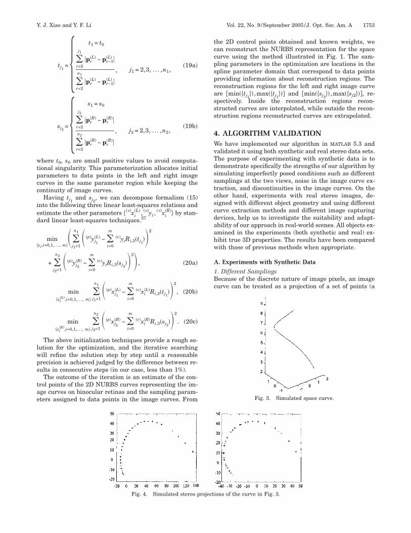

wtpcc

ied

�

lwps

tae

tccpsprasss

4WvTdsstoscdaahw

A

1Bc


tj1=�

t1 = t0

�r=2

j1

�pr�L� − pr−1

�L� �

�r=2

n1

�pr�L� − pr−1

�L� �

, j1 = 2,3, . . . ,n1,� �19a�

sj2=�

s1 = s0

�r=2

j2

�pr�R� − pr

�R��

�r=2

n2

�pr�R� − pr

�R��

, j2 = 2,3, . . . ,n2,� �19b�

here t0, s0 are small positive values to avoid computa-ional singularity. This parameterization allocates initialarameters to data points in the left and right imageurves in the same parameter region while keeping theontinuity of image curves.

Having tj1and sj2

, we can decompose formalism (15)nto the following three linear least-squares relations andstimate the other parameters ��xi

�L� , ��yi ,��xi

�R�� by stan-ard linear least-squares techniques.27

minyi,i=0,1,. . ., m�

��j1=1

n1 ��p�yj1�L� − �

i=0

m�v�yiRi,3�tj1

��2

+ �j2=1

n2 ��p�yj2�R� − �

i=0

m�v�yiRi,3�sj2

��2� , �20a�

min�xi

�L�,i=0,1,. . ., m��j1=1

n1 ��p�xj1�L� − �

i=0

m�v�xi

�L�Ri,3�tj1��2

, �20b�

min�xi

�R�,i=0,1,. . ., m��j2=1

n2 ��p�xj2�R� − �

i=0

m�v�xi

�R�Ri,3�sj2��2

. �20c�

The above initialization techniques provide a rough so-ution for the optimization, and the iterative searchingill refine the solution step by step until a reasonablerecision is achieved judged by the difference between re-ults in consecutive steps (in our case, less than 1%).

The outcome of the iteration is an estimate of the con-rol points of the 2D NURBS curves representing the im-ge curves on binocular retinas and the sampling param-ters assigned to data points in the image curves. From

Fig. 4. Simulated stereo p

he 2D control points obtained and known weights, wean reconstruct the NURBS representation for the spaceurve using the method illustrated in Fig. 1. The sam-ling parameters in the optimization are locations in thepline parameter domain that correspond to data pointsroviding information about reconstruction regions. Theeconstruction regions for the left and right image curvere min��tj1

�� ,max��tj1�� and min��sj2

�� ,max��sj2��, re-pectively. Inside the reconstruction regions recon-tructed curves are interpolated, while outside the recon-truction regions reconstructed curves are extrapolated.

. ALGORITHM VALIDATIONe have implemented our algorithm in MATLAB 5.3 and

alidated it using both synthetic and real stereo data sets.he purpose of experimenting with synthetic data is toemonstrate specifically the strengths of our algorithm byimulating imperfectly posed conditions such as differentamplings at the two views, noise in the image curve ex-raction, and discontinuities in the image curves. On thether hand, experiments with real stereo images, de-igned with different object geometry and using differenturve extraction methods and different image capturingevices, help us to investigate the suitability and adapt-bility of our approach in real-world scenes. All objects ex-mined in the experiments (both synthetic and real) ex-ibit true 3D properties. The results have been comparedith those of previous methods when appropriate.

. Experiments with Synthetic Data

. Different Samplingsecause of the discrete nature of image pixels, an imageurve can be treated as a projection of a set of points (a

Fig. 3. Simulated space curve.

ions of the curve in Fig. 3.
roject

sorpcnmcpet

iep=

�t=ipavml

Fb


ampling) in 3D on a continuous curve. For a stereo pairf image curves, unless specifically designed, the left andight image curves are usually cast from different sam-lings on the 3D curve. Therefore precise point-to-pointorrespondence matching can hardly be achieved in itsature, even without noise in images. In our first experi-ent, we evaluated our algorithm with simulated image

urves whose data points correspond to different sam-lings on a 3D free-form curve. To this end, we first gen-rated a ground-truth curve in 3D using parametric equa-ions:

��t� � � X = 2 cos t

Y = 2 sin t t � 0,5/4�

Z = 2�t + 1�� .

Such a curve is truly spatial (nonplanar) as illustratedn Fig. 3. We sampled this curve uniformly in the param-ter region by an interval of tint=� /24, giving 31 samplingoints on the curve. We denoted these parameters by tt1 , . . . t31 and the corresponding sampling points by

Table 1. Errors of Reconstruction

Approach �t=0.1tint

NURBS-based

e3d= �0.00720.01510.000275100.0038

�b

e2dl= �0.13610.70780.00420.1192

�e2dr= �0.0966

0.44350.00520.0759

�Point-based

e3d= �0.02800.10180.00320.0260

�e2dl= �0.1626

0.55080.01330.1459

�e2dr= �0.1285

0.43680.01320.0953

�ae3d, e2dl, e2dr denote errors in 3D, left retina, and rightbEach column vector contains the values of mean, max

�t�. We then added Gaussian white noise to t and ob-ained another parameter set t�= t1� , . . . t31� such that ti�ti+n�0,�t�, i=1,2, . . . ,31, where n�0,�t� denotes Gauss-

an noise with zero mean and standard deviation �t. Werojected the sampling points ��t� onto the left retinand the sampling points ��t�� onto the right retina in airtual parallel stereo configuration, where the projectionatrices of left and right cameras were designed as fol-

ows:

h Sampling Differences, in Pixels

oise Levels

�t=0.2tint �t=0.3tint

0.00750.01460.000150310.0037

� e3d= � 0.00790.0160

0.000308960.0036

�2dl= �0.1402

0.59670.00170.1214

� e2dl= �0.14540.59760.00320.1188

�2dr= �0.0990

0.36540.00220.0733

� e2dr= �0.10440.36370.00370.0717

�e3d= �0.0573

0.16440.00640.0437

� e3d= �0.08780.33470.00800.0823

�2dl= �0.2257

1.02270.03550.2009

� e2dl= �0.28611.23630.03890.2674

�2dr= �0.1764

0.69860.03220.1278

� e2dr= �0.24070.84160.00840.1998

�espectively.

inimum, and SD in descending order.

ig. 5. 3D reconstruction from projections in Fig. 4. (a) Point-ased, (b) NURBS-based.

a wit

N

e3d= �e

e

e

e

retina, r

imum, m

Td�atTisT

Tbostpewaac

rSpsgcwrg1ms0pl

wlmsb

trcfcspinvtNwscs

2Iios1cbaormcptb


T�L� = 100 0 0 1

0 100 0 0

0 0 1 1�, T�R� = 100 0 0 − 1

0 100 0 0

0 0 1 1� .

If the standard deviation of noise �t=0, then the point�L��ti�� on the left retina must be the exact correspon-ence of the point T�R��ti�� on the right retina, because�ti� and ��ti�� are the same samplings in 3D. When we

ssign a positive value to �t, the sampling difference be-ween two image curves appears. If we still treat�L��ti�� and T�R��ti�� as a stereo pair of correspond-

ng points, an error will occur in the location of the corre-pondences. Figure 4 illustrates the stereo projections�L��ti�� and T�R��ti�� when �t=0.3tint.Using the corresponding pairs T�L��ti�� and

�R��ti��, i=1,2, . . . ,31, we can reconstruct 31 3D pointsy triangulation. Figure 5(a) shows a linear interpolationf these reconstructed points, which makes it easy to vi-ualize the recovered shape of the curve. It is shown thathe reconstruction result is strongly affected by the sam-ling difference between the two image curves. The recov-red 3D curve is neither smooth nor accurate. In contrast,ith our algorithm a much better result has beenchieved as illustrated in Fig. 5(b). The recovered curve islmost the same as the original one in Fig. 3, with sevenontrol points in its NURBS representation.

The quantitative measurements of reconstruction er-ors, conducted in both 3D and 2D, are listed in Table 1.ince we know the ground-truth curve in 3D, we can com-ute closest point distances (CPDs)37 from the recon-tructed curve (in the reconstruction region) to theround-truth curve, which reflect proximity of the twourves. The 2D measurement is conducted in a similaray, i.e., by computing CPDs from the projections of the

econstructed curve (in left and right reconstruction re-ions) to the projections of the ground-truth curve. Tablelists four significant statistics of these CPDs, i.e., theean values, maximum values, minimum values, and

tandard deviations (SD) under noise levels �t=0.1tint,.2tint, and 0.3tint. Applying the same measurements tooint-based reconstruction results, we obtained the dataisted in the second row of Table 1.

Obviously the NURBS-based reconstruction is over-helmingly better than point-based reconstruction in at

east two respects. First, in precision, the maxima,eans, and standard deviations of NURBS-based recon-

truction errors are much smaller than those of point-ased results in both 3D and 2D. Second, in consistency,

Fig. 6. Corrupted stereo projections ��= 0.6�0.6T� of the c

he NURBS-based method achieves a similar quality ofeconstruction results when the samplings of imageurves vary, showing its insensitivity to the sampling dif-erence, whereas the point-based approach produces re-onstruction errors clearly associated with the levels ofampling differences. Actually in the NURBS-based ap-roach, optimal positions are assigned to all data pointsn terms of sampling parameters on the spline, which areot necessarily required to be the same at left and rightiews, while the point-based approach relies crucially onhe location precision of point correspondences. ThereforeURBS-based reconstruction is truly “curve-based,”hich means it needs no correspondence and permits

ampling differences between data points in imageurves, while the point-based method is particularly con-trained to the matching accuracy of data points.

. Noisy Datan the second experiment, we validated our algorithm us-ng image curves corrupted by random noise. Without lossf generality, we used Gaussian white noise again toimulate the random noise in curve extraction. Sampling00 points uniformly along each projected curve of the 3Durve in Fig. 3 (this means that the interval on the curveetween any pair of adjacent points is identical), wedded 2D Gaussian noise n�0,�� to the coordinate vectorsf these points. In Fig. 6 the jagged curves are the cor-upted image curves ��= 0.6 0.6T�. We can observeany sharp glitches along the image curves that strongly

hange the local properties of the curves. If we apply aoint-based approach to this kind of data, accurate point-o-point correspondences will be extremely hard to findecause of the noise. However, using the NURBS-based

Fig. 3 and the back projections of the reconstructed curve.

Fig. 7. Reconstructed curve from corrupted stereo projections.

urve in

asvrw

ittlct0i

soipsaawpba

3Fpoitre3spftwm3Fcsoapscw

ascsptt

vi


lgorithm, we can obtain an acceptable reconstruction re-ult as shown in Fig. 7, where the reconstructed curve isery close to the original 3D curve. The projections of oureconstructed curve are shown in Fig. 6 as smooth curves,hich obviously fit well to the image curves.The quantitative analysis of the reconstruction errors

s given in Table 2 using the same measuring method ashat in the first experiment. On the whole the reconstruc-ion errors are relatively small compared with the noiseevels, as noise is suppressed by the introduction of theurve model. At the highest noise level ��= 1.0 1.0T�,he mean of reconstruction errors in 2D is about.2 pixels, while the induced noise reaches about 1.0 pixeln each image axis on average. The quantitative data also

Table 2. Errors of Reconstructiona with CorruptedData, in Pixels

Noise Level e3d e2dl e2dr

�= 0.2 0.2T

�0.01190.02860.00200.0043

�b �0.19520.78120.00830.1558

� �0.13540.55490.00410.0995

��= 0.4 0.4T

�0.01620.07210.00280.0198

� �0.19680.76870.00490.1486

� �0.13610.55960.01300.1042

��= 0.6 0.6T

�0.02600.08920.00280.0198

� �0.19240.80900.01640.1272

� �0.17770.55550.10090.0260

��= 0.8 0.8T

�0.04830.15750.00290.0398

� �0.19010.81860.01050.1498

� �0.18390.52800.01790.0987

��= 1.0 1.0T

�0.06740.40810.00910.0639

� �0.20690.78340.02550.1704

� �0.20860.58850.02670.1470

�ae3d, e2dl, e2dr denote errors in 3D, left retina, and right retina, respectively.bEach column vector contains the values of mean, maximum, minimum, and SD

n descending order.

Fig. 8. Broken stereo pr

how that the reconstruction errors in 2D exhibit no signf an apparent increase when stronger noise is induced,ndicating the stability of our algorithm in randomly-osed noisy conditions according to our reconstruction as-umption: finding the 3D curve which best fits the 2D im-ge data. The 3D reconstruction errors appear to increases noise increases. The reason is that the stronger noiseill cause larger stereo ambiguity around curve partsarallel to epipolar lines. We will explain the stereo am-iguity further in the experiments with real stereo im-ges below.

. Fragmented Curvesragmented curves commonly occur at the early-visionrocessing stage of real images as a result of deficienciesf both image data and curve extraction methods, whichndeed brings considerable difficulty to the reconstruc-ion. As it is based on the NURBS curve model, our algo-ithm can potentially deal with this problem to a certainxtent. Figure 8 illustrates a pair of stereo images of theD curve in Fig. 3 that consist of data points uniformlyampled on the exact projections of the curve with somearts missing. Each missing part is randomly selectedrom an original projection with its length being 1/10 ofhe whole length of the projected curve. We assume thate still know the order of curve segments in the frag-ented curves. For instance, we know fragments 1, 2, andin Fig. 8(a) are successive segments of an image curve.eeding our algorithm with such fragmented imageurves, the result is a continuous and smooth curve ashown in Fig. 9, which resembles rather accurately theriginal 3D curve in Fig. 3. As our algorithm reconstructs

curve as a whole and retains the continuity of dataoints, missing parts in one image curve can be compen-ated for by the corresponding parts in the other imageurve. Table 3 lists the quantitative reconstruction errors,hich clearly remain quite low in both 3D and 2D cases.We compared the result with that of the B-spline-based

pproach26 (in second row, Table 3), which also recon-tructs a curve as a whole. It is clearly seen that the re-onstruction error level of the NURBS-based method isignificantly lower than that of the B-spline-based ap-roach, indicating that the NURBS model represents (in-erpolates and extrapolates) data points more accuratelyhan the B-spline approach in the fragmented case.

The above three experiments with synthetic data re-ealed certain strengths of our method: It is not sensitive

ns of the curve in Fig. 3.
ojectio

tar

BTtwgjsasm

vfcpettctawstaot

A

N

B

i

Fig. 9. Reconstructed curve from data in Fig. 8.


o different samplings in stereo images, it works reason-bly well in noisy conditions, and it has the potential forecovering missing parts of measured curves.

. Experiments with Real Imageshe purpose of experiments with real data is to examine

he suitability and adaptability of the approach in real-orld scenes. In the experiments we have used tworoups of real stereo images acquired from different sub-ects in different scenes at different times using differenttereo capturing devices. In the first experiment, the im-ging device used was a narrow-baseline stereo head con-isting of two B/W cameras calibrated with the projectionatrices identified as follows:

T�L� = 16.2 0.3 4.5 − 1455.9

1 − 16.6 2.5 773.7

− 0.3 − 0.2 − 1 538.1� ,

T�R� = 16.1 0.3 4.4 − 2042.6

− 0.4 − 16.5 2.6 980.8

0.3 − 0.2 − 1 510.3� .

The objects of interest are the boundaries of the threeanes of a fan model (Fig. 10), which exhibit true 3D free-orm properties suitable for our tests. Each of these threeurves was modeled by a NURBS curve with 23 controloints from image curves extracted using the Canny op-rator. Figure 11 displays the reconstructed curves athree orthogonal views. Curves 1, 2, and 3 are the 3D con-ours of the three vanes that appear from the bottomounter clockwise in the stereo images. The back projec-ions of the reconstructed curves to the binocular retinasre displayed as curves marked by white x’s in Fig. 10,here we can clearly see that the reconstructed 3D

hapes of the fan-vanes produce projections that fit well tohe image contours of the fan. In sharp contrast, when wepplied straight line primitives for 3D reconstruction, webtained the much cluttered result shown in Figure 12 athe same orthogonal views, indicating again the appropri-

ack projections of the reconstruction result.

Table 3. Errors of Reconstructiona withFragmented Data, in Pixels

pproach e3d e2dl e2dr

URBS-based

� 0.00770.0148

4.9422�10−0.005

0.0039�b �0.1999

0.54550.00140.1805

� �0.13300.52260.00120.1070

�-Spline-based

�0.58121.19260.00870.4052

� �2.31536.32770.04501.7830

� �1.22882.42780.01990.6562

�ae3d, e2dl, e2dr denote errors in 3D, left retina, and right retina, respectively.bEach column vector contains the values of mean, maximum, minimum, and SD

n descending order.

Fig. 10. Real stereo images of a fan model and b

acf

wbmaca(rtBptt

tapaeplrdtIstt

r1al

Fsigco

weTw

scaccscbcte

jts

segme


teness of choosing NURBS as shape representation andomputing a curve as a whole for reconstructing 3D, free-orm curved objects.

As there is no ground-truth curve in this experiment,e measure only quantitative reconstruction errors of theack projections in 2D, listed in Table 4. The measure-ents are distances between data points in image curves

nd their corresponding points on the projected NURBSurves (the spline parameter for each data point is knownfter reconstruction). We use the same four statisticsmean, maximum, minimum, and standard deviation) toepresent the distances. In order to prove our hypothesishat the NURBS-based approach is superior to the-spline-based approach,26 we conducted the same ex-eriment with the latter approach using the same quan-itative measurements and compared the results of thewo approaches.

The statistical data in Table 4 reveal the difference be-ween the reconstruction results obtained from the twopproaches. While the NURBS-based method yield sub-ixel level reconstruction errors with the largest error inll six projected curves of less than 1.1 pixels and the av-rage CPD less than 0.22 pixels, the B-spline-based ap-roach produces pixel level reconstruction errors with theargest error as much as 9.5 pixels. The relatively largeeconstruction errors in the B-spline-based approach areue mainly to the nonotimized sampling parameters andhe affine approximation of perspective transformation.n the NURBS-based approach, on the other hand, theampling parameters are optimized and a fully perspec-ive camera model is adopted, which dramatically reduceshe reconstruction errors.

Careful readers might notice the small distortion occur-ing in the reconstructed curve 1 shown in Figs. 11(b) and1(c). The distortion is caused by stereo ambiguity, whichrises when part of an image curve overlaps an epipolarine [see the horizontal white line just above the bottom of

Fig. 11. Reconstruct

Fig. 12. Reconstructed line

ig. 10(a)]. In such a condition, the variation of a recon-tructed 3D curve on an epiolar plane will yield no changen its projections on the binocular retinas. Such an ambi-uity is due to the nature of triangulation itself, and itan be dealt with by introducing more constraints in theptimization framework.

In the second experiment, the stereo images in Fig. 13ere taken by a B/W camera mounted on a manipulator’snd effector at two different positions at different times.he projection matrices in such a stereo configurationere calibrated as

T�L� = − 2.5465 1.6975 − 14.6749 90.1389

2.8606 21.9431 0.5021 − 6414.6

− 0.0176 0.0065 − 0.0022 1� ,

T�R� = 8.3536 − 1.3601 8.5493 − 4096.7

− 2.1115 − 17.6109 0.9637 4891.9

0.0127 − 0.0052 − 0.0065 1� .

The objects of interest were two wires bent in complexhapes in 3D space. Our purpose was to reconstruct theurves representing the skeletons of the wires. We appliedNURBS curve model with 13 control points for the short

urve and 23 control points for the long curve. The imageurves were extracted using region segmentation andkeleton extraction techniques.38 The reconstructedurves using our approach are shown in Fig. 14, and theirack projections to two binocular retinas are displayed asurves marked by white x’s in Fig. 13. It is evident thathe result visually exhibits a quality similar to that in thexperiment with the fan model.

The quantitative reconstruction errors of the back pro-ections of the bentwire objects using our approach andhe B-spline-based approach are listed in Table 5 (thehort and long curves are labeled as curve 1 and curve 2,

ves of the fan model.

nts of fan model in Fig. 10.

ed cur

ralpp

pctosTa

edheuosMfi

odtttpo

N

B

i


espectively), where the NURBS-based approach stillchieves subpixel accuracy compared with the ratherarge reconstruction errors in the B-spline-based ap-roach, basically reproducing the results of our first ex-eriment.It is also worth mentioning that in the above two ex-

eriments with real data, the imaging devices, the stereoonfigurations, the image curve extraction methods, andhe shapes and sizes of objects are all different from eachther. Nevertheless, the NURBS-based method does nothow significant difference in the quality of the results.his fact points up the potential suitability and adapt-bility of the approach in real applications.Figures 15 and 16 illustrate residual errors in the it-

rative processes of the above two experiments with realata. Obviously the iterative processes converged at veryigh rates. In a few iteration steps, the resulting residualrrors dropped to a very low level and remain virtuallynchanged thereafter. This observation reveals that thebjective function formulated in our optimization has aharp slope around the optimal solution. The Levenberg–arquardt approach can then quickly follow the slope to

nd the solution zones.Figure 17 illustrates the change of control points in the

ptimization for one curve (curve 2 in Fig. 10(a)). Theashed curve is the image curve, and the circles are con-rol points of the NURBS curve that represent it. Theraces of control points are depicted as the short curves inhe upper left-hand corner of Fig. 17(b), with the initialositions represented by crosses. From the enlarged partf the curve in Fig. 17(a), we can clearly see that the

s of the reconstructed curves. (a) Left image, (b) right image.

s of bent wire objects.

Table 4. Reconstruction Errorsa of the Fan Model,in Pixels

Approach Curve 1 Curve 2 Curve 3

URBS-based

e2dl= �0.20950.83840.00160.1872

�b e2dl= �0.21291.00260.00540.1700

� e2dl= � 0.05920.4045

0.000704600.0677

�e2dr= �0.1957

0.68010.00230.1541

� e2dr= �0.23040.83920.00280.1813

� e2dr= � 0.06960.3640

0.000303070.0744

�-Spline based

e2dl= �2.20894.94370.00951.7267

� e2dl= �1.87974.34700.01301.9866

� e2dl= �1.88499.50690.02682.2086

�e2dr= �1.9709

4.58740.01581.5445

� e2dr= �1.79974.55490.00372.0025

� e2dr= �1.78649.55560.01402.2680

�ae2dl, e2dr denote errors in left retina and right retina, respectively.bEach column vector contains the values of mean, maximum, minimum, and SD

n descending order.

Fig. 13. Stereo images of bent wire objects and the back projection

Fig. 14. Reconstructed curve

ceptctpctmts

mtfar

5IafcgOem

rorisridsrm

raasnaBs

attlcb

N

B

i


hange of control points is large in the first few steps—specially in the first step—and afterwards the controloints remain stable. This result agrees with the observa-ion drawn from Fig. 15. Moreover, the overall domain ofhange of control points is relatively small compared withhe size of the whole image, implying that the normalizedarameterization for data points can provide roughly ac-eptable results (with pixel level reconstruction errorshat are only as large as those of the B-spline-basedethod as given in Tables 4 and 5) and serve as good ini-

ialization of sampling parameters in the optimization. Ithould also be noted that in the above real-world experi-

Table 5. Reconstruction Errorsa of the Bent WireObjects, in Pixels

Approach Curve 1 Curve 2

URBS-based

e2dl= �0.30790.89920.00070.1993

�b e2dl= �0.36631.42990.00140.2815

�e2dr= �0.2657

0.88350.00190.2013

� e2dr= �0.34671.92140.00040.2849

�-spline based

e2dl= � 4.821144.99630.04478.9624

� e2dl= �2.52318.86610.00401.6836

�e2dr= � 3.4315

34.31480.04094.8338

� e2dr= � 2.403011.82370.01391.9952

�ae2dl, e2dr denote errors in left retina and right retina, respectively.bEach column vector contains the values of mean, maximum, minimum, and SD

n descending order.

Fig. 15. Residual errors with iterat

ents, all objects chosen are of a true 3D nature, showinghe capability of our algorithm of reconstructing 3D free-rom curves from images, while our method can certainlylso be applied to planar objects, as NURBS is a unifiedepresentation of curves.

. CONCLUDING REMARKSn this paper, we have presented a scheme to reconstructNURBS representation of a 3D, free-form curve directly

rom its stereo images. Previously, curve-based stereo re-onstruction methods were either restricted to planar al-ebraic curves or constrained to an affine camera model.ur approach advances such technique by allowing bothntirely 3D free-form curves and a perspective cameraodel while requiring no point-to-point correspondences.Based on the perspective invariance of the NURBS rep-

esentation, we have deduced constraints on a stereo pairf projections of a space NURBS curve and formulated theeconstruction into an optimization framework. Throughts smooth representation of curves, NURBS leads to thehape parameters of the NURBS model and sampling pa-ameters for the data points being globally differentiablen the energy function, thereby permitting the use oferivative-based optimization techniques in the recon-truction. While the algorithm needs no explicit point cor-espondence, the data points themselves are actuallyatched to optimal positions on the NURBS curves.Our experiments revealed that the approach is able to

econstruct 3D curves from their images on digital retinasrbitrarily sampled and permits randomly-posed noisend partial missing data while yielding much better re-ults than the B-spline-based method. With the sameumber of control points, the NURBS-based approachchieved subpixel accuracy of reconstruction, whereas the-spline-based method achieved only pixel-level preci-ion.

The NURBS-based reconstruction framework can bepplied to various vision applications where curve pat-erns construct the major information cue to understandhe 3D scene, e.g., surface reconstruction from structuredights. NURBS representation imposes no constraint onurve shapes, therefore suiting a large range of curve-ased applications, particularly in natural environments.

reconstructing curves of fan model.
ions in

Aeesc

taasi

AL2tl

wj

nal

Sf

Lc


ddressing the full implications of NURBS in shape mod-ling is beyond the scope of the research here; the inter-sted readers can refer to the latest literature39,40 totudy other issues such as the selection of the number ofontrol points.

Finally, noting that the current scheme constructed inhe sheer least-squares measure does not resolve stereombiguity (as illustrated in Fig. 10), we are consideringccommodating more constraints, e.g., structural con-traints, in our NURBS-based optimization framework tomprove further the reconstruction quality.

PPENDIX A: PROOF OF THEOREM 2et C�t�= X�t� ,Y�t� ,Z�t�T denote a 3D NURBS curve. ItsD projection c�t�= x�t� ,y�t�T can be expressed by func-ions of the 3D control points Vi and weights Wi as fol-ows, using Eqs. (1), (3), and (5):

�x�t� = �i=0

m

T1�Vi

1 �Ri,k�t��i=0

m

T3�Vi

1 �Ri,k�t�

y�t� = �i=0

m

T2�Vi

1 �Ri,k�t��i=0

m

T3�Vi

1 �Ri,k�t�� ,

here T1, T2, T3 are row vectors in the perspective pro-ection matrix and R �t� are rational basis functions.

Fig. 16. Residual errors with iterations

Fig. 17. Trace of control points in

i,k

Simultaneously multiplying the numerator and de-ominator of the right side of the first equation of thebove equation array by a factor of �j=0

m WjBj,k�t�, the fol-owing equation results:

x�t� = �i=0

m

T1�Vi

1 �WiBi,k�t��i=0

m

T3�Vi

1 �WiBi,k�t�.

Thus

x�t� = �i=0

m T1�Vi

1 �T3�Vi

1 �T3�Vi


m

T3�Vi

1 �WiBi,k�t�.

imilarly, we can deduce the following equation for y�t�rom the second equation of the equation array:

y�t� = �i=0

m T2�Vi

1 �T3�Vi

1 �T3�Vi


m

T3�Vi

1 �WiBi,k�t�.

et vi=T�Vi� and wi=T3Vi

1Wi. The above two equations

an then be rewritten in a vector form:

onstructing curves of bent wire objects.

timization of curve 2 in Fig. 10(a).

in rec

the op

Oc

ATg(Mc

R

1

1

1

1

1

1

1

1

1

1

2

2

2

2

2

2

2

2

2

2

3

3

3

3

3

3

3

3

3

3

4


c�t� = �i=0

m

wiviBi,k�t��i=0

m

wiBi,k�t�

wi = WiT3�Vi

1 � .

bviously, the projected curve c�t� is a NURBS curve withontrol points of vi and weights of wi.

Theorem 2 is thus proved.

CKNOWLEDGMENTShe work described in this paper was fully supported by arant from the Research Grants Council of Hong KongProject CityU1130/03E). The authors thank J. P. Siebert,

. Ding, F. M. Wahl, and the reviewers for their usefulomments and help with the research.

EFERENCES1. O. Faugeras, Three-dimensional Computer Vision: a

Geometric Viewpoint (MIT Press, 1993).2. D. Scharstein and R. Szeliski, “Taxonomy and evaluation of

dense two-frame stereo correspondence algorithms,” Int. J.Comput. Vis. 47, 7–42 (2002).

3. M. Z. Brown, D. Burschka, and G. D. Hager, “Advances incomputational stereo,” IEEE Trans. Pattern Anal. Mach.Intell. 25, 993–1008 (2003).

4. M. Pollefeys and S. Sinha, “Iso-disparity surfaces forgeneral stereo configurations,” presented at the EighthEuropean Conference on Computer Vision, Prague, CzechRepublic, May 11–14, 2004.

5. M. H. Lin and C. Tomasi, “Surfaces with occlusions fromlayered stereo,” IEEE Trans. Pattern Anal. Mach. Intell.26, 1073–1078 (2004).

6. O. Faugeras and R. Keriven, “Variational principles,surface evolution, PDEs, level-set methods, and the stereoproblem,” IEEE Trans. Image Process. 7, 336–344 (1998).

7. N. Ayache and F. Lustman, “Trinocular stereo vision forrobotics,” IEEE Trans. Pattern Anal. Mach. Intell. 13,73–85 (1991).

8. D. Q. Huynh and R. A. Owens, “Line labeling and region-segmentation in stereo image pairs,” Image Vis. Comput.12, 213–225 (1994).

9. G. Pajares, J. M. Cruz, and J. A. Lopez-Orozco, “Stereomatching using Hebbian learning,” IEEE Trans. Syst. ManCybern. 29, 553–559 (1999).

0. N. Ayache and B. Faverjon, “Efficient registration of stereoimages by matching graph descriptions of edge segments,”Int. J. Comput. Vis. 1, 107–131 (1987).

1. S. D. Ma, “Conic-based stereo, motion estimation, and posedetermination,” Int. J. Comput. Vis. 10, 7–25 (1993).

2. L. Quan, “Conic reconstruction and correspondence fromtwo views,” IEEE Trans. Pattern Anal. Mach. Intell. 18,151–160 (1996).

3. L. Li and S. D. Ma, “3D pose estimation from a N-degreeplanar curve in two perspective views,” presented at the13th International Conference on Pattern Recognition,Vienna, Austria, August 25–30, 1996.

4. M. H. An and C. N. Lee, “Stereo vision based on algebraiccurves,” presented at the 13th International Conference onPattern Recognition, Vienna, Austria, August 25–30, 1996.

5. L. Robert and O. D. Faugeras, “Curve-based stereo: figuralcontinuity and curvature,” presented at the InternationalConference on Computer Vision and Pattern Recognition,Maui, Hawaii, June 3–6, 1991.

6. K. Kedem and Y. Yarmovski, “Curve based stereo matchingusing the minimum Hausdorff distance,” presented at the12th Symposium on Computational Geometry,Philadelphia, Pennsylvania, May 24–26, 1996.

7. A. T. Brant and M. Brady, “Stereo matching of curves byleast deformation,” presented at the InternationalWorkshop on Intelligent Robots and Systems ’89, Tsukuba,Japan, September 4–6, 1989.

8. N. M. Nasrabadi, “A stereo vision technique using curvesegments and relaxation matching,” IEEE Trans. PatternAnal. Mach. Intell. 14, 566–572 (1992).

9. N. M. Nasrabadi and Y. Liu, “Stereo vision correspondenceusing a multi-channel graph matching technique,” ImageVis. Comput. 7, 237–245 (1989).

0. G. Pajares, J. M. Cruz, and J. A. Lopez-Orozco, “Relaxationlabeling in stereo image matching,” Pattern Recogn. 33,53–68 (2000).

1. J. Porrill and S. Pollard, “Curve matching and stereocalibration,” Image Vis. Comput. 9, 45–50 (1991).

2. Y. Shan and Z. Zhang, “New measurements and corner-guidance for curve matching with probabilistic relaxation,”Int. J. Comput. Vis. 46, 157–171 (2002).

3. C. Schmid and A. Zisserman, “The geometry and matchingof lines and curves over multiple views,” Int. J. Comput.Vis. 40, 199–233 (2000).

4. J. Sato and R. Cipolla, “Quasi-invariant parameterisationsand matching of curves in images,” Int. J. Comput. Vis. 28,117–136 (1998).

5. R. Berthilsson, K. Astrom, and A. Heyden, “Reconstructionof general curves using factorization and bundleadjustment,” Int. J. Comput. Vis. 41, 171–182 (2002).

6. Y. J. Xiao, M. Y. Ding, and J. X. Peng, “B-spline basedstereo for 3D reconstruction of line-like objects using affinecamera model,” Int. J. Pattern Recognit. Artif. Intell. 15,347–358 (2001).

7. D. F. Rogers and N. G. Fog, “Constrained B-spline curveand surface fitting,” Comput. Aided Des. 21, 641–648(1989).

8. S. Hu, Y. Li, T. Ju, and X. Zhu, “Modifying the shape ofNURBS surfaces with geometric constraints,” Comput.-Aided Des. 33, 903–912 (2001).

9. H. Qin and D. Terzopoulos, “D-NURBS: a physics-basedframework for geometric design,” IEEE Trans. Vis.Comput. Graph.2, 85–96 (1996).

0. F. S. Cohen and J. Y. Wang, “Modeling image curves usinginvariant 3D curve models—a path to 3D recognition andshape estimation from image contours,” IEEE Trans.Pattern Anal. Mach. Intell. 16, 1–12 (1994).

1. L. Piegl, “On NURBS: a survey,” IEEE Comput. GraphicsAppl. 13(1), 55–71 (1991).

2. J. Aloimonos, “Perspective approximations,” Image Vis.Comput. 8, 179–192 (1990).

3. N. Ayache and C. Hansen, “Rectification of images forbinocular and trinocular stereovision,” presented at the 9thInternational Conference on Pattern Recognition, Beijing,China, November 14–17, 1988.

4. W. Ma and J.-P. Kruth, “NURBS curve and surface fittingfor reverse engineering,” Int. J. Adv. Manuf. Technol. 14,918–927 (1998).

5. D. W. Marquardt, “An algorithm for least-squaresestimation of nonlinear parameters,” J. Soc. Ind. Appl.Math. 11, 431–441 (1963).

6. W. H. Press, B. P. Flannery, S. A. Teukolsky, and W. T.Vetterling, Numerical Recipes in C: The Art of ScientificComputing, 2nd ed. (Cambridge U. Press, 1992), pp.681–688.

7. P. J. Besl and N. D. McKay, “A method for registration of3-d shapes,” IEEE Trans. Pattern Anal. Mach. Intell. 14,239–256 (1992).

8. R. M. Haralick and L. G. Shapiro, Computer and RobotVision (Addison-Wesley, 1992), Vol. I, pp. 233–236.

9. H. P. Yang, W. P. Wang, and J. G. Sun, “Control pointadjustment for B-spline curve approximation,” Comput.Aided Des. 36, 639–652 (2004).

0. T. J. Cham and R. Cipolla, “Automated B-spline curverepresentation incorporating MDL and error-minimizingcontrol point insertion strategies,” IEEE Trans. PatternAnal. Mach. Intell. 21, 49–53 (1999).

optimized stereo reconstruction of free-form space curves based on a nonuniform rational b-spline...

Documents