arX

iv:1

410.

8633

v1 [

cs.N

I] 3

1 O

ct 2

014

1

Optimized Distributed Inter-cell InterferenceCoordination (ICIC) Scheme using ProjectedSubgradient and Network Flow Optimization

Akram Bin Sediq, Rainer Schoenen, Halim Yanikomeroglu, andGamini Senarath

Abstract— In this paper, we tackle the problem of multi-cell resource scheduling, where the objective is to maximizethe weighted sum-rate through inter-cell interference coordi-nation (ICIC). The blanking method is used to mitigate theinter-cell interference, where a resource is either used with apredetermined transmit power or not used at all, i.e., blanked.This problem is known to be strongly NP-hard, which meansthat it is not only hard to solve in polynomial time, but it isalso hard to find an approximation algorithm with guaranteedoptimality gap. In this work, we identify special scenarioswherea polynomial-time algorithm can be constructed to solve thisproblem with theoretical guarantees. In particular, we define adominant interference environment, in which for each user thereceived power from each interferer is significantly greater thanthe aggregate received power from all other weaker interferers.

We show that the originally strongly NP-hard problem canbe tightly relaxed to a linear programming problem in adominant interference environment. Consequently, we propose apolynomial time distributed algorithm that is not only guar anteedto be tight in a dominant interference environment, but whichalso computes an upper bound on the optimality gap withoutadditional computational complexity. The proposed schemeisbased on the primal-decomposition method, where the problemis divided into a master-problem and multiple subproblems.We solve the master-problem iteratively using the projected-subgradient method. We also show that each subproblem hasa special network flow structure. By exploiting this networkstructure, each subproblem is solved using the network-based op-timization methods, which significantly reduce the complexity incomparison to the general-purpose convex or linear optimizationmethods. In comparison with baseline schemes, simulation resultsof the International Mobile Telecommunications-Advanced(IMT-Advanced) scenarios show that the proposed scheme achieveshigher gains in aggregate throughput, cell-edge throughput, andoutage probability.

Index Terms—Multi-cell scheduling, convex optimization,inter-cell interference coordination (ICIC), distribute d algo-rithms, efficiency-fairness tradeoff

I. I NTRODUCTION

Aggressive reuse is inevitable in cellular networks due tothe scarcity of the radio resources. Reuse-1, in which allradio resources are reused in every sector, is an example of

A. Bin Sediq, R. Schoenen, and H. Yanikomeroglu are with the Departmentof Systems and Computer Engineering, Carleton University,Ottawa, ON,Canada (e-mail:{akram, rs, halim}@sce.carleton.ca).

G. Senarath is with Huawei Technologies Canada Co., Ltd. (e-mail:gamini.senarath@huawei.com).

This work is supported in part by Huawei Canada Co., Ltd., in part bythe Ontario Ministry of Economic Development and Innovation’s ORF-RE(Ontario Research Fund - Research Excellence) program, andin part byan Ontario Graduate Scholarship in Science and Technology (OGSST). Apreliminary version of this work was presented at IEEE PIMRC2011 [1].

such an aggressive frequency reuse scheme. While reuse-1can potentially achieve high aggregate system throughput,itjeopardizes the throughput experienced by users close to thecell1-edge, due to the excessive interference experienced bythese users. Therefore, it is vital for the network to use robustand efficient interference mitigation techniques.

Conventionally, interference is mitigated by static resourcepartitioning and frequency/sector-planning, where close-bysectors are assigned orthogonal resources (clustering). Acommon example is reuse-3 (cluster size = 3 sectors) [2,Section 2.5], where adjacent sectors are assigned orthogo-nal channels, i.e., there is no inter-cell interference betweenadjacent sectors. Although such techniques can reduce inter-cell interference and improve cell-edge user throughput, theysuffer from two major drawbacks. First of all, the aggregatenetwork throughput is significantly reduced since each sectorhas only a fraction of the available resources, which is equalto the reciprocal of the reuse factor. Secondly, conventionalfrequency/sector-planning may not be possible in emergingwireless networks where new multi-tier network elements(such as relays, femto-/pico-base-stations, distributedantennaports) are expected to be installed without prior planning inself-organizing networks (SON) [3].

In order to reduce the effect of the first drawback, fractionalfrequency reuse (FFR) schemes have been proposed. The keyidea in FFR is to assign lower reuse factor for users near thecell-center and higher reuse factor for users at the cell-edge.The motivation behind such a scheme is that cell-edge usersare more vulnerable to inter-cell interference than cell-centerusers. Soft Frequency Reuse (SFR) [4] and Partial FrequencyReuse (PFR) [5] are two examples of FFR. A comparativestudy between reuse-1, reuse-3, PFR, and SFR is provided in[6], [7]. While FFR schemes recover some of the throughputloss due to partitioning, they require frequency/sector planninga priori, which is not desirable in future cellular networksasmentioned earlier. As a result, developing efficient dynamicinter-cell interference coordination (ICIC) schemes is vital tothe success of future cellular networks [3].

One approach to tackle the ICIC problem is to deviseadaptive FFR or SFR schemes. In [8], an adaptive FFR schemeis proposed where each base-station (BS) chooses one of

1The terms “cell” and “sector” are used interchangeably in this work.

2

several reuse modes. A dynamic and centralized2 FFR schemeis proposed in [9] that outperforms conventional FFR schemesin terms of the total system throughput. In [10], the authorspropose softer frequency reuse, which is a heuristic algorithmbased on modifying the proportional fair algorithm and theSFR scheme. In [11], a heuristic algorithm based on adaptiveSFR is proposed for the uplink. In [12], the authors proposegradient-based distributed schemes that create SFR patterns, inan effort to achieve local maximization of the network utility.To enable gradient computation, the rate adaptation functionthat maps signal-to-interference-and-noise-ratio (SINR) to rateis required to be differentiable. However, this requirementis not currently feasible since rate adaption is performedin current cellular standards by using adaptive modulationand coding (AMC) with a discrete set of modulation andcoding schemes [13], which results in a non-differentiablerateadaptation function.

Another approach to tackle the ICIC problem is to removethe limitations imposed by the FFR schemes and view theICIC problem as a multi-cell scheduling problem. In [14],the authors propose a suboptimal centralized algorithm wherea radio network controller is assumed to be connected toall BSs. The authors conclude that the problem is NP-hardand they resort to heuristics that show improvement in theperformance. In [15], a graph-theoretic approach is takento develop an ICIC scheme in which information about theinterference experienced by each user terminal (UT) is inferredfrom the diversity set of that UT. In [16], a game-theoretic ap-proach is pursued and an autonomous decentralized algorithmis developed. The proposed algorithm converges to a Nashequilibrium in a simplified cellular system. Nevertheless,asignificant gap is observed between the proposed algorithmand the globally optimum one, which is computationallydemanding. In [3], a partly distributed two-level ICIC schemeis proposed where a centralized entity is required to solvea binary linear optimization problem, which is generally notsolvable in polynomial time.

The focus of this paper is to overcome the drawbacks of theexisting schemes mentioned above by developing a distributedICIC scheme, that can work with any AMC scheme, and yetprovide theoretical guarantee. In particular, we tackle the prob-lem of distributed multi-cell resource scheduling, where theobjective is to maximize the weighted sum-rate. The blankingmethod is used to mitigate the inter-cell interference, where aresource is either used with a predetermined transmit poweror not used at all, i.e., blanked, similar to [3]. This problem isknown to be strongly NP-hard, which means that it is not onlyhard to solve in polynomial time, but it is also hard to find anapproximation algorithm with guaranteed optimality gap [17].The main contributions can be summarized as follows:

1) We show that the originally strongly NP-hard problemcan be tightly relaxed to a linear programming problemin a dominant interference environment, in which for

2In this paper, an algorithm is categorized as a centralized algorithm if itrequires a centralized entity to coordinate or to perform either partial or fullexecution of the algorithm. In contrast, a distributed algorithm is one thatcan be executed in each sector with limited message exchangebetween thesectors, without the requirement of having a centralized entity.

each user the received power from each interferer issignificantly greater than the aggregate received powerfrom all other weaker interferers3. The tightness of therelaxation is shown by proving that the percentage ofoptimal relaxed variables that assume binary values isbounded below by K(M−1)

(K+1)M+1· 100%, whereM is the

average number of UTs per sector andK is the numberof neighboring interferers. Consequently, we devise apolynomial-time distributed algorithm that is not onlyguaranteed to be tight, but which also computes anupper bound on the optimality gap without additionalcomputational complexity. The proposed algorithm doesnot require a central controller and it can be used withany AMC scheme, including AMC schemes that result innon-differentiable discrete rate adaption functions.

2) We demonstrate that considered optimization problem fora dominant interference environment can be transformedinto an equivalent minimum-cost network flow (MCNF)optimization problem. Thus, we can use network-basedalgorithms which have significantly reduced complexityas compared to the general-purpose convex or linearoptimization algorithms [18, p. 402]. While MCNF op-timization tools have been used in the literature to solveresource allocation problem in single-cell networks, e.g.,[19] and [20], as far as we know, our work is the first inliterature to use these optimization tools in ICIC, i.e., inmulti-cell resource allocation problems.

II. SYSTEM MODEL

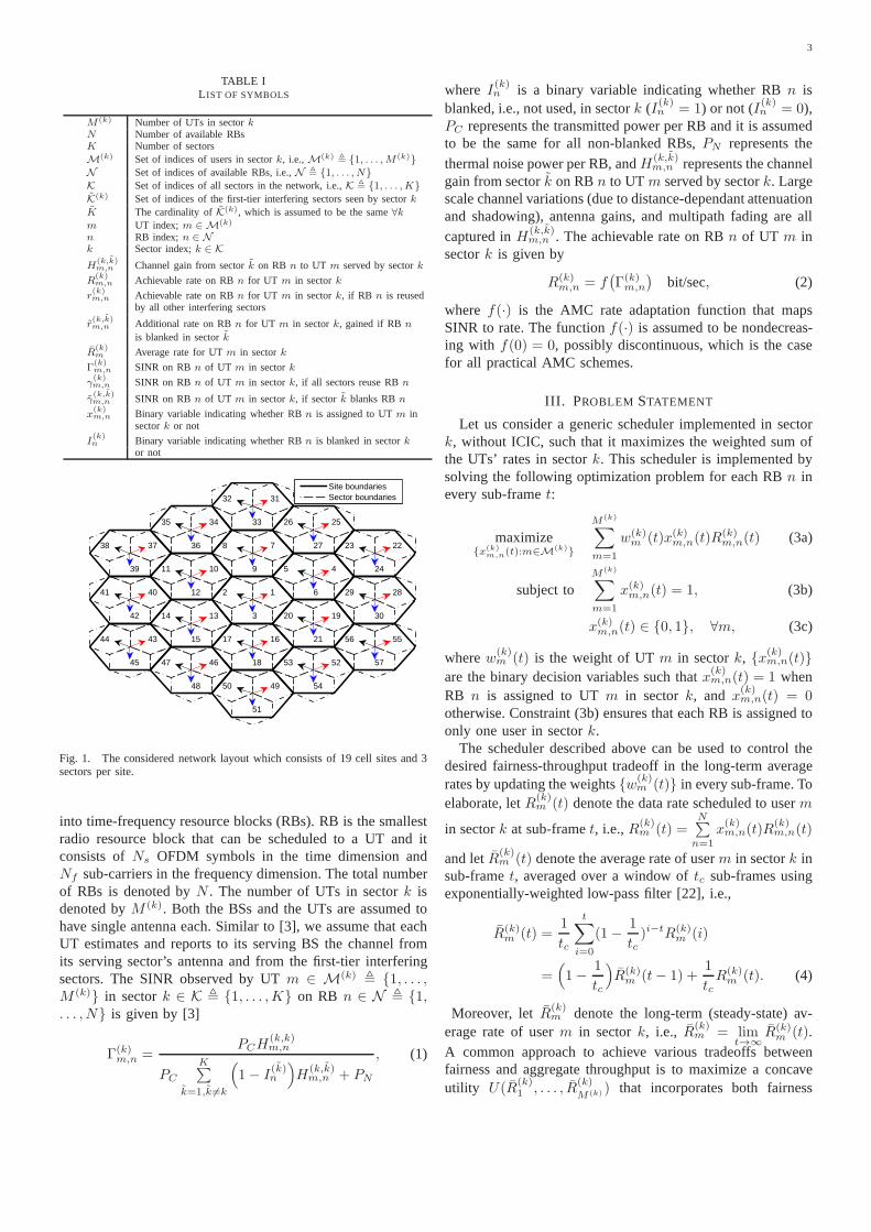
We consider the network model described by theInternational Mobile Telecommunications-Advanced (IMT-Advanced) evaluation guidelines [21]. Based on these guide-lines, the considered network consists ofK sectors servedby K/3 BSs as shown in Fig. 1. Each BS is equipped witha tri-sector antenna to serve a cell-site that consists of 3sectors. Each BS can communicate with its neighboring BSs;this is supported in most cellular network standards, e.g.,using the R8 interface in IEEE 802.16m standard and the X2interface in Long-Term Evolution (LTE) and LTE-advancedstandards. Hexagonal sectors are considered herein accord-ing to IMT-Advanced guidelines; nevertheless, the proposedscheme works also for arbitrary sector shapes. We focus on thedownlink scenario in this paper. For convenience, the symbolsused in this section and onward are provided in Table I.

Orthogonal Frequency Division Multiple Access (OFDMA)is used as the multiple access scheme, since it is adoptedin most of the contemporary cellular standards. Among theadvantages offered by OFDMA is its scheduling flexibility,since users can be scheduled in both time and frequency,which can be exploited to gain time, frequency, and multi-userdiversity. The time and frequency radio resources are grouped

3The definition of a dominant interference environment is illustrated bythe following example. Assume there are four interferers, and let Pr(k)

denote the received power from thekth interferer. Assume further thatPr(1) > Pr(2) > Pr(3) > Pr(4). Such an environment is called adominant interference environment if and only if the following conditions aresatisfied:Pr(1) >> Pr(2) + Pr(3) + Pr(4), Pr(2) >> Pr(3) + Pr(4),andPr(3) >> Pr(4).

3

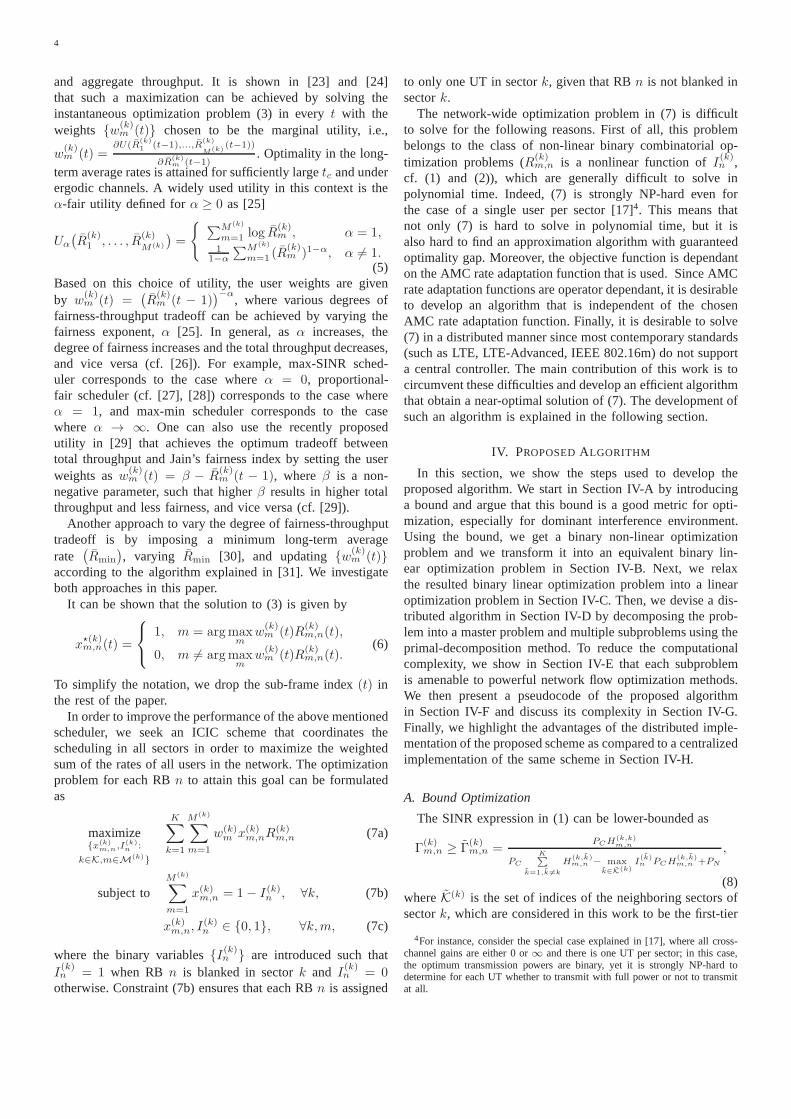
TABLE IL IST OF SYMBOLS

M (k) Number of UTs in sectorkN Number of available RBsK Number of sectorsM(k) Set of indices of users in sectork, i.e.,M(k) , {1, . . . ,M (k)}N Set of indices of available RBs, i.e.,N , {1, . . . , N}K Set of indices of all sectors in the network, i.e.,K , {1, . . . ,K}K(k) Set of indices of the first-tier interfering sectors seen by sectorkK The cardinality ofK(k), which is assumed to be the same∀km UT index; m ∈ M(k)

n RB index;n ∈ Nk Sector index;k ∈ K

H(k,k)m,n Channel gain from sectork on RBn to UT m served by sectork

R(k)m,n Achievable rate on RBn for UT m in sectork

r(k)m,n Achievable rate on RBn for UT m in sectork, if RB n is reused

by all other interfering sectors

r(k,k)m,n Additional rate on RBn for UT m in sectork, gained if RBn

is blanked in sectork

R(k)m Average rate for UTm in sectork

Γ(k)m,n SINR on RBn of UT m in sectork

γ(k)m,n SINR on RBn of UT m in sectork, if all sectors reuse RBn

γ(k,k)m,n SINR on RBn of UT m in sectork, if sector k blanks RBn

x(k)m,n Binary variable indicating whether RBn is assigned to UTm in

sectork or not

I(k)n Binary variable indicating whether RBn is blanked in sectork

or not

12

3

45

6

78

91011

12

1314

15 1617

18

1920

21

2223

24

2526

27

2829

30

3132

333435

363738

39

4041

42

4344

45 4647

48 4950

51

5253

54

5556

57

Site boundariesSector boundaries

Fig. 1. The considered network layout which consists of 19 cell sites and 3sectors per site.

into time-frequency resource blocks (RBs). RB is the smallestradio resource block that can be scheduled to a UT and itconsists ofNs OFDM symbols in the time dimension andNf sub-carriers in the frequency dimension. The total numberof RBs is denoted byN . The number of UTs in sectork isdenoted byM (k). Both the BSs and the UTs are assumed tohave single antenna each. Similar to [3], we assume that eachUT estimates and reports to its serving BS the channel fromits serving sector’s antenna and from the first-tier interferingsectors. The SINR observed by UTm ∈ M(k) , {1, . . . ,M (k)} in sectork ∈ K , {1, . . . ,K} on RB n ∈ N , {1,. . . , N} is given by [3]

Γ(k)m,n =

PCH(k,k)m,n

PC

K∑

k=1,k 6=k

(

1− I(k)n

)

H(k,k)m,n + PN

, (1)

where I(k)n is a binary variable indicating whether RBn is

blanked, i.e., not used, in sectork (I(k)n = 1) or not (I(k)n = 0),PC represents the transmitted power per RB and it is assumedto be the same for all non-blanked RBs,PN represents the

thermal noise power per RB, andH(k,k)m,n represents the channel

gain from sectork on RBn to UT m served by sectork. Largescale channel variations (due to distance-dependant attenuationand shadowing), antenna gains, and multipath fading are allcaptured inH(k,k)

m,n . The achievable rate on RBn of UT m insectork is given by

R(k)m,n = f

(

Γ(k)m,n

)

bit/sec, (2)

where f(·) is the AMC rate adaptation function that mapsSINR to rate. The functionf(·) is assumed to be nondecreas-ing with f(0) = 0, possibly discontinuous, which is the casefor all practical AMC schemes.

III. PROBLEM STATEMENT

Let us consider a generic scheduler implemented in sectork, without ICIC, such that it maximizes the weighted sum ofthe UTs’ rates in sectork. This scheduler is implemented bysolving the following optimization problem for each RBn inevery sub-framet:

maximize{x(k)

m,n(t):m∈M(k)}

M(k)∑

m=1

w(k)m (t)x(k)

m,n(t)R(k)m,n(t) (3a)

subject toM(k)∑

m=1

x(k)m,n(t) = 1, (3b)

x(k)m,n(t) ∈ {0, 1}, ∀m, (3c)

wherew(k)m (t) is the weight of UTm in sectork, {x(k)

m,n(t)}

are the binary decision variables such thatx(k)m,n(t) = 1 when

RB n is assigned to UTm in sectork, and x(k)m,n(t) = 0

otherwise. Constraint (3b) ensures that each RB is assignedtoonly one user in sectork.

The scheduler described above can be used to control thedesired fairness-throughput tradeoff in the long-term averagerates by updating the weights{w(k)

m (t)} in every sub-frame. Toelaborate, letR(k)

m (t) denote the data rate scheduled to userm

in sectork at sub-framet, i.e.,R(k)m (t) =

N∑

n=1

x(k)m,n(t)R

(k)m,n(t)

and letR(k)m (t) denote the average rate of userm in sectork in

sub-framet, averaged over a window oftc sub-frames usingexponentially-weighted low-pass filter [22], i.e.,

R(k)m (t) =

1

tc

t∑

i=0

(1−1

tc)i−tR(k)

m (i)

=(

1−1

tc

)

R(k)m (t− 1) +

1

tcR(k)

m (t). (4)

Moreover, letR(k)m denote the long-term (steady-state) av-

erage rate of userm in sectork, i.e., R(k)m = lim

t→∞R(k)

m (t).A common approach to achieve various tradeoffs betweenfairness and aggregate throughput is to maximize a concaveutility U(R

(k)1 , . . . , R

(k)

M(k)) that incorporates both fairness

4

and aggregate throughput. It is shown in [23] and [24]that such a maximization can be achieved by solving theinstantaneous optimization problem (3) in everyt with theweights {w

(k)m (t)} chosen to be the marginal utility, i.e.,

w(k)m (t) =

∂U(R(k)1 (t−1),...,R

(k)

M(k)(t−1))

∂R(k)m (t−1)

. Optimality in the long-

term average rates is attained for sufficiently largetc and underergodic channels. A widely used utility in this context is theα-fair utility defined forα ≥ 0 as [25]

Uα

(

R(k)1 , . . . , R

(k)

M(k)

)

=

{

∑M(k)

m=1 log R(k)m , α = 1,

11−α

∑M(k)

m=1 (R(k)m )1−α, α 6= 1.

(5)Based on this choice of utility, the user weights are givenby w

(k)m (t) =

(

R(k)m (t − 1)

)−α, where various degrees of

fairness-throughput tradeoff can be achieved by varying thefairness exponent,α [25]. In general, asα increases, thedegree of fairness increases and the total throughput decreases,and vice versa (cf. [26]). For example, max-SINR sched-uler corresponds to the case whereα = 0, proportional-fair scheduler (cf. [27], [28]) corresponds to the case whereα = 1, and max-min scheduler corresponds to the casewhere α → ∞. One can also use the recently proposedutility in [29] that achieves the optimum tradeoff betweentotal throughput and Jain’s fairness index by setting the userweights asw(k)

m (t) = β − R(k)m (t − 1), whereβ is a non-

negative parameter, such that higherβ results in higher totalthroughput and less fairness, and vice versa (cf. [29]).

Another approach to vary the degree of fairness-throughputtradeoff is by imposing a minimum long-term averagerate

(

Rmin

)

, varying Rmin [30], and updating{w(k)m (t)}

according to the algorithm explained in [31]. We investigateboth approaches in this paper.

It can be shown that the solution to (3) is given by

x⋆(k)m,n(t) =

1, m = argmaxm

w(k)m (t)R

(k)m,n(t),

0, m 6= argmaxm

w(k)m (t)R

(k)m,n(t).

(6)

To simplify the notation, we drop the sub-frame index(t) inthe rest of the paper.

In order to improve the performance of the above mentionedscheduler, we seek an ICIC scheme that coordinates thescheduling in all sectors in order to maximize the weightedsum of the rates of all users in the network. The optimizationproblem for each RBn to attain this goal can be formulatedas

maximize{x(k)

m,n,I(k)n :

k∈K,m∈M(k)}

K∑

k=1

M(k)∑

m=1

w(k)m x(k)

m,nR(k)m,n (7a)

subject toM(k)∑

m=1

x(k)m,n = 1− I(k)n , ∀k, (7b)

x(k)m,n, I

(k)n ∈ {0, 1}, ∀k,m, (7c)

where the binary variables{I(k)n } are introduced such thatI(k)n = 1 when RBn is blanked in sectork and I

(k)n = 0

otherwise. Constraint (7b) ensures that each RBn is assigned

to only one UT in sectork, given that RBn is not blanked insectork.

The network-wide optimization problem in (7) is difficultto solve for the following reasons. First of all, this problembelongs to the class of non-linear binary combinatorial op-timization problems (R(k)

m,n is a nonlinear function ofI(k)n ,cf. (1) and (2)), which are generally difficult to solve inpolynomial time. Indeed, (7) is strongly NP-hard even forthe case of a single user per sector [17]4. This means thatnot only (7) is hard to solve in polynomial time, but it isalso hard to find an approximation algorithm with guaranteedoptimality gap. Moreover, the objective function is dependanton the AMC rate adaptation function that is used. Since AMCrate adaptation functions are operator dependant, it is desirableto develop an algorithm that is independent of the chosenAMC rate adaptation function. Finally, it is desirable to solve(7) in a distributed manner since most contemporary standards(such as LTE, LTE-Advanced, IEEE 802.16m) do not supporta central controller. The main contribution of this work is tocircumvent these difficulties and develop an efficient algorithmthat obtain a near-optimal solution of (7). The developmentofsuch an algorithm is explained in the following section.

IV. PROPOSEDALGORITHM

In this section, we show the steps used to develop theproposed algorithm. We start in Section IV-A by introducinga bound and argue that this bound is a good metric for opti-mization, especially for dominant interference environment.Using the bound, we get a binary non-linear optimizationproblem and we transform it into an equivalent binary lin-ear optimization problem in Section IV-B. Next, we relaxthe resulted binary linear optimization problem into a linearoptimization problem in Section IV-C. Then, we devise a dis-tributed algorithm in Section IV-D by decomposing the prob-lem into a master problem and multiple subproblems using theprimal-decomposition method. To reduce the computationalcomplexity, we show in Section IV-E that each subproblemis amenable to powerful network flow optimization methods.We then present a pseudocode of the proposed algorithmin Section IV-F and discuss its complexity in Section IV-G.Finally, we highlight the advantages of the distributed imple-mentation of the proposed scheme as compared to a centralizedimplementation of the same scheme in Section IV-H.

A. Bound Optimization

The SINR expression in (1) can be lower-bounded as

Γ(k)m,n ≥ Γ

(k)m,n =

PCH(k,k)m,n

PC

K∑

k=1,k 6=k

H(k,k)m,n − max

k∈K(k)I(k)n PCH

(k,k)m,n +PN

,

(8)whereK(k) is the set of indices of the neighboring sectors ofsectork, which are considered in this work to be the first-tier

4For instance, consider the special case explained in [17], where all cross-channel gains are either 0 or∞ and there is one UT per sector; in this case,the optimum transmission powers are binary, yet it is strongly NP-hard todetermine for each UT whether to transmit with full power or not to transmitat all.

5

interfering sectors seen by sectork; e.g., in Fig. 1,K(3) = {1,2, 13, 17, 16, 20}5. The cardinality ofK(k) is assumed to bethe same for all sectors and it is denoted byK, i.e., |K(k)| =K, ∀k. The bound in (8) is obtained by assuming that RBnis used in all sectors, except at most one sector. When RBn is blanked in more than one interfering sector, only themost dominant blanked interferer is considered6. This boundis exact if the number of blanked interferers is less or equalto one and it is tight for small number of blanked interferers.The bound is also tight for dominant interference environment,where the received power from each interferer to each user issignificantly greater than the aggregate received power fromall other weaker interferers.

The bound in (8) is a good metric to be used for opti-mization (maximization) for the following reasons. First ofall, if the bound is increased by∆, then the exact expressiongiven by (1) will also increase by at least∆ (proof is given inAppendix A). Moreover, it is already observed in the literaturethat blanking a particular RB in more than two sectors candegrade the overall system performance (cf. [3]). Finally,andmost importantly, based on this bound, we can develop adistributed optimization framework that is applicable to awiderange of schedulers and AMC strategies for dominant interfer-ence environments. This framework can be implemented veryefficiently, and can achieve near-optimal performance, as wewill see later.

Using the SINR bound given in (8), we now construct asimilar bound on the rates,{R(k)

m,n}, given in (2). To do so,we defineγ(k)

m,n andr(k)m,n as the SINR and the correspondingachievable rate on RBn of UT m in sectork, if all sectorsuse RBn, i.e.,

γ(k)m,n =

PCHk,km,n

PC

∑

k 6=k

H(k,k)m,n + PN

, r(k)m,n = f(

γ(k)m,n

)

. (9)

Similarly, we defineγ(k,k)m,n and r

(k,k)m,n as the SINR and the

additional rate on RBn of UT m in sectork, if only sectork ∈ K(k) blanks RBn, i.e.,

γ(k,k)m,n =

PCH(k,k)m,n

PC

∑

k 6=k

Hk,km,n−PCH

(k,k)m,n +PN

,

r(k,k)m,n = f

(

γ(k,k)m,n

)

− r(k)m,n.

(10)

Using the definitions ofγ(k)m,n andγ(k,k)

m,n given in (9) and (10),respectively, the SINR bound given by (8) can be also writtenas

Γ(k)m,n ≥ Γ(k)

m,n = max(

γ(k)m,n,max

k

I(k)n γ(k,k)m,n

)

, (11)

where the equivalence between (8) and (11) stems from the

fact that{I(k)n } assume binary values.

5We assume a wraparound layout so each sector has 6 first-tier interferingsectors; e.g.,K(25) = {26, 27, 23, 51, 50, 48}.

6Note that this bound considers the most dominantblanked interferer whichis not necessarily the most dominant interferer when the most dominantinterferer does not blank RBn (i.e., when it is not turned off). Thisdifferentiates (8) from the expression considered in [14],where the mostdominant interferer is considered.

Using (9) and (10), a bound on the rates,{R(k)m,n}, given by

(2) is constructed based on the SINR bound given by (11) as

R(k)m,n = f(Γ

(k)m,n) ≥ f(Γ

(k)m,n)

= f(

max(

γ(k)m,n,maxk I

(k)n γ

(k,k)m,n

))

= max(

r(k)m,n,maxk I

(k)n (r

(k)m,n + r

(k,k)m,n )

)

= r(k)m,n + max

k∈K(k)

I(k)n r

(k,k)m,n ,

(12)where the first equality follows from (2), the first inequalityand the second equality follow from (11) and the fact thatf(·)is assumed to be nondecreasing, the third equality follows from(9), (10), and the fact thatf(·) is assumed to be nondecreasingwith f(0) = 0, and the fourth equality follows from the factthat r(k)m,n is not a function ofk.

The physical meaning of the bound in (12) is similar to theSINR bound in (8)–the rate bound is obtained by assumingthat RB n is used in all sectors, except at most one sector.When RBn is blanked in more than one interfering sector,only the most dominant blanked interferer is considered.

By substituting (12) in (7), the optimization problem in (7)can be tightly approximated for dominant interference envi-ronment as

maximize{x(k)

m,n,I(k)n :

k∈K,m∈M(k)}

K∑

k=1

M(k)∑

m=1

w(k)m x(k)

m,n

(

r(k)m,n + maxk∈K(k)

I(k)n r(k,k)m,n

)

(13a)

subject toM(k)∑

m=1

x(k)m,n = 1− I(k)n , ∀k, (13b)

x(k)m,n, I

(k)n ∈ {0, 1}, ∀k,m. (13c)

The optimization problem (13) is a non-linear binary integeroptimization problem, which is in general, difficult to solve.As an intermediate step to reduce the complexity of solving(13), we convert it to an equivalent binary linear optimizationproblem in the following section.

B. Transforming (13) Into an Equivalent Binary Linear Opti-mization Problem

Our approach to tackle the binary non-linear optimizationproblem given by (13) is to first transform it into an equivalentbinary linear optimization problem. While binary linear opti-mization problems are still not easy to solve in general, goodapproximate solutions can be computed efficiently by relaxingthe constraints that restrict the variables to be either 0 or1,into weaker constraints that restrict the variables to assume anyreal value in the interval[0, 1]. The challenge is to constructan equivalent binary linear optimization problem that has atight relaxation which means that the solution obtained bysolving the relaxed version is very close to the one obtainedbysolving the binary linear optimization problem. This challengeis addressed in this section.

In order to convert the binary non-linear optimization prob-lem given by (13) into an equivalent binary linear optimizationproblem, we need to convert the termx(k)

m,n maxk∈K(k)

I(k)n r

(k,k)m,n

6

into a linear term. There are two sources of non-linearity inthis term: the point-wise maximum and the multiplication. Thenon-linear term can be written as

x(k)m,n max

k∈K(k)

I(k)n r(k,k)m,n = maxy(k,k)m,n ∈C

∑

k∈K(k)

y(k,k)m,n r(k,k)m,n , (14)

where the variables{y(k,k)m,n : k ∈ K, k ∈ K(k),m ∈ M(k),n ∈ N} are introduced as auxiliary variables that facilitatethe conversion of the non-linear term into a linear term and

C ={

y(k,k)m,n :

∑

k∈K(k)

y(k,k)m,n ≤ 1, ∀k,m,

y(k,k)m,n ≤ x

(k)m,n, ∀k, k,m,

y(k,k)m,n ≤ I

(k)n , ∀k, k,m,

y(k,k)m,n ∈ {0, 1}, ∀k, k,m

}

.

(15)

To see the equivalence, we note that since all variablesassume binary values, then the point-wise maximum in theoriginally non-linear term is captured in (14) and the firstinequality in (15). Moreover, the multiplication in the orig-inally non-linear term is captured in the second and the thirdinequalities in (15).

By replacing the termx(k)m,n max

k∈K(k)I(k)n r

(k,k)m,n in (13a) with

(14) and (15), we get an equivalent binary linear optimizationproblem. Unfortunately, we found experimentally that suchanequivalent optimization problem leads to loose linear relax-ation, i.e., it results in solutions that are far from the binaryoptimal solutions. As a result, we seek tighter equivalentformulations.

A general approach to get tighter relaxation is by addingadditional constraints that are called valid constraints [32, p.585]. These valid constraints do not change the set of feasiblebinary solutions; however, with proper choice of these validconstraints, one can obtain tighter relaxations. Based on thisapproach, we construct a setC′ that is equivalent toC for theconsidered binary optimization problem, by adding two validconstraints:

∑

k∈K(k) y(k,k)m,n ≤ x

(k)m,n, ∀k,m,

∑M(k)

m=1 y(k,k)m,n ≤ I

(k)n , ∀k, k.

(16)

Hence,C′ is given by

C′ ={

y(k,k)m,n :

∑

k∈K(k) y(k,k)m,n ≤ x

(k)m,n, ∀k,m,

∑M(k)

m=1 y(k,k)m,n ≤ I

(k)n , ∀k, k,

y(k,k)m,n ∈ {0, 1}, ∀k, k,m

}

.

(17)Note that the constraintsy(k,k)m,n ≤ x

(k)m,n and y

(k,k)m,n ≤ I

(k)n ,

given originally in (15), are omitted from the definition ofC′

given in (17) since these constraints define a subset of the firsttwo constraints given in (17). The equivalence ofC andC′ isprovided in the following Lemma.

Lemma 1. The sets C and C′ given by (15) and (17),respectively, are equivalent.

Proof: See Appendix B.

By replacing the termx(k)m,n max

k

I(k)n r

(k,k)m,n in (13) with

(14) and (17), we get the following binary linear optimizationproblem7:

maximize{x(k)

m,n,y(k,k)m,n ,I(k)

n :

k∈K,k∈K(k),m∈M(k)}

K∑

k=1

M(k)∑

m=1

w(k)m

(

x(k)m,nr

(k)m,n

+∑

k∈K(k)

y(k,k)m,n r(k,k)m,n

)

(18a)

subject toM(k)∑

m=1

x(k)m,n = 1− I(k)n , ∀k, (18b)

∑

k∈K(k)

y(k,k)m,n ≤ x(k)m,n, ∀k,m, (18c)

M(k)∑

m=1

y(k,k)m,n ≤ I(k)n , ∀k, k, (18d)

x(k)m,n, y

(k,k)m,n , I(k)n ∈ {0, 1}, ∀k, k,m.

(18e)

We finally remark that many other equivalent binary opti-mization problems can be formulated, e.g., by replacing thetermx

(k)m,n max

k

I(k)n r

(k,k)m,n in (13) with (14) and (15). However,

different equivalents will have different relaxations. Unlikemany other equivalent formulations, the relaxed version oftheformulation in (18) has the following advantages:

• The optimal solution is provably close to binary as wewill show in Section IV-C.

• It can be readily solved in distributed manner usingprimal decomposition as we will show in Section IV-D.

• It can be solved efficiently using network flow optimiza-tion tools as we will show in Section IV-E.

C. Linear Optimization Relaxation

An upper bound on the optimum value of (18) can beobtained by solving the relaxed version of (18) which can beconstructed by replacing (18e) with the following constraints

x(k)m,n, y

(k,k)m,n , I(k)n ∈ [0, 1], ∀k ∈ K, k ∈ K(k),m ∈ M(k).

(19)In particular, letp⋆Binary denote the optimal value of (18), letp⋆Relaxeddenote the optimal value of the relaxed version of (18),and let p⋆Relaxed denote the value of the objective functionevaluated at a rounded-solution of the relaxed problem, suchthat the rounded solution is a feasible binary solution of (18).Then, we have the following inequalities

p⋆Relaxed≥ p⋆Binary ≥ p⋆Relaxed, (20)

where the first inequality follows from the fact that the feasibleset of the relaxed version is always a superset of the originalproblem and the second equality follows directly from the

7Note that themax operator in the right-hand side of (14) is omittedfrom the objective of the optimization problem in (18), since the optimizationproblem is already a maximization problem.

7

optimality of p⋆Binary. We define the optimality gap,∆Opt, inpercentage as

∆Opt =(

p⋆Binary − p⋆Relaxed

)

/p⋆Binary·100%≤(

p⋆Relaxed− p⋆Relaxed

)

/p⋆Relaxed·100%,(21)

where the inequality follows from (20). Thus, one can computean estimate on the optimality gap in polynomial time bysolving a linear optimization problem. As we will show inSection VI-A through extensive simulations, by solving therelaxed problem and rounding the solution to the closest binaryfeasible solution, one can obtain a solution to (18) that is near-optimal, i.e., with small∆Opt.

An important objective measure of the tightness of a relax-ation is the percentage of optimal relaxed variables that assumebinary values. For instance, the optimality gap goes to zeroasthis percentage goes to 100%. We now provide a closed-formtheoretical guarantee on the this percentage. This theoreticalguarantee is summarized in the following proposition.

Proposition 1. The percentage of optimal variables of therelaxed version of (18) that assume binary values is greaterthan or equal to K(M−1)

(K+1)M+1· 100%, where M is the average

number of UTs per sector and K is the number of neighboringinterferers.

Proof: See Appendix C.For example, ifM (k) = 20, ∀k, and K = 6, then using

Proposition 1 we can deduce that the percentage of optimalvariables of the relaxed version of (18) that assume binaryvalues is guaranteed to be greater than or equal to 80.8%.

However, solving the relaxed problem would require acentral controller to be connected to all the BSs in order tosolve a large linear optimization problem. Such a central con-troller is not supported in most contemporary cellular networkstandards, such as LTE, LTE-Advanced and IEEE 802.16m.Consequently, we seek in the following section a distributedoptimization method to solve the relaxed version of problem(18).

D. Primal Decomposition

The relaxed version of (18) has a special separable structure.In particular, for any set of fixed{I(k)n , ∀k ∈ K}, it can beseparated intoK optimization problems, each can be solvedseparately in each sector. In this section, we show how thisstructure is exploited to develop a distributed algorithm basedon the primal-decomposition method8 [33, pp. 3–5].

To exploit the separable structure, letφ(k)(I(1)n , . . . , I

(K)n )

denote the optimal value of the following optimization prob-lem for given{I(1)n , . . . , I

(K)n }:

maximize{x(k)

m,n,y(k,k)m,n :

m∈M(k),k∈K(k)}

M(k)∑

m=1

w(k)m

(

x(k)m,nr

(k)m,n +

∑

k∈K(k)

y(k,k)m,n r(k,k)m,n

)

(22a)

8Primal-decomposition is considered in this paper instead of dual-decomposition since the structure is readily separable in the primal domain.Moreover, since the objective function is not strictly concave, recovering theoptimal primal variables from optimal dual variables can bechallenging fordual-decomposition method [33, p. 4].

subject toM(k)∑

m=1

x(k)m,n = 1− I(k)n , (22b)

∑

k∈K(k)

y(k,k)m,n ≤ x(k)m,n, ∀m, (22c)

M(k)∑

m=1

y(k,k)m,n ≤ I(k)n , ∀k, (22d)

x(k)m,n, y

(k,k)m,n ,∈ [0, 1], ∀m, k. (22e)

For reasons that will become apparent, we call (22) subprob-lem k. Using (22), the relaxed version of (18) is equivalent to

maximizeI(k)n ,k∈K

K∑

k=1

φ(k)(I(1)n , . . . , I(K)n ) (23a)

subject to I(k)n ∈ [0, 1], ∀k ∈ K. (23b)

We call (23) the master problem. Therefore, the relaxedversion of (18) has been decomposed into a master problem,given by (23), andK subproblems, each is given by (22) andcan be solved separately in each sector.

The master problem given in (23) is a convex optimizationproblem with a concave objective function of the variables{I

(1)n , . . . , I

(K)n } and a convex constraint set, since the re-

laxed version of (18) is a linear (thus convex) optimizationproblem (cf. [33, p. 2]). Since the objective is not necessarilydifferentiable, the projected-subgradient method can be usedto solve this problem iteratively [34, p. 16]. In each iteration,K subproblems are solved in each sector in order to evaluateφ(k)(I

(1)n , . . . , I

(K)n ), ∀k ∈ K, and subgradients[Λ⋆(1)

n , . . . ,

Λ⋆(K)n ] ∈ ∂

∑K

k=1 φ(k)(I

(1)n , . . . , I

(K)n ), where ∂f(x) is the

subdifferential off(·) evaluated atx. To explain how thesubgradients[Λ⋆(1)

n , . . . ,Λ⋆(K)n ] are obtained, letg(k)n (f(x))

denote thekth element of a subgradient of the functionf(·)evaluated atx for RB n. Using the definition of a subgradient(cf. [35, p. 1]), it is not difficult to see thatg(k)n is closed underaddition, and thus,

Λ⋆(k)n = g

(k)n (∑K

k=1 φ(k)(I

(1)n , . . . , I

(K)n ))

=∑K

k=1 g(k)n (φ(k)(I

(1)n , . . . , I

(K)n )).

(24)

As shown in [33, p. 5],g(k)n (φ(k)(I(1)n , . . . , I

(K)n )) can be

obtained from an optimum lagrange multiplier (dual variable)that corresponds to the constraint whereI

(K)n appears in its

right-hand-side. Consequently,Λ⋆(k)n can be explicitly written

asΛ⋆(k)n := −λ⋆(k)

n +∑

k∈K(k)

λ⋆(k,k)n , (25)

whereλ⋆(k)n is an optimum Lagrange multiplier corresponding

to constraint (22b) andλ⋆(k,k)n , k ∈ K(k), are optimum

Lagrange multipliers corresponding to constraints (22d).In order for each sectork to calculateΛ⋆(k)

n , it requiresthe knowledge ofλ⋆(k)

n , which can be obtained locally by

solving (22), andλ⋆(k,k)n , k ∈ K(k), which can be exchanged

from the neighboring sectors. In other words, each sectork

sendsλ(k,k)n for all k sectors that are in the neighborhood

8

of sectork, for all n. The master algorithm then updates itsvariables as

I(k)n := I(k)n + δΛ(k)n , ∀k ∈ K, (26)

whereδ is the step-size which can be chosen using any of thestandard methods given in [34, pp. 3–4]. Then, eachI

(k)n is

projected into the feasible set of[0, 1] as follows

I(k)n :=

0, I(k)n ≤ 0,

I(k)n , 0 < I

(k)n < 1,

1, I(k)n ≥ 1.

(27)

Using (25), (26), and (27), each sectork can compute thevariables{I(k)n , ∀n ∈ N} in a distributed manner without theneed for a centralized entity. Then, each sectork exchangesI(k)n with its neighbors and the process is repeated forNiter

iterations. After that, eachI(k)n is rounded to the nearest binaryvalue which is denoted byI⋆(k)n . Once{I⋆(k)n } are determined,local scheduling decision variables{x⋆(k)

m,n} can be determinedin each sectork separately as follows. For everym ∈ M(k),

n ∈ N , R(k)m,n is calculated using (1), (2), andI⋆(k)n . To

ensure feasibility of the resulting solution to problem (18),the scheduling decision variables are calculated as

x⋆(k)m,n =

1, m = argmaxm

w(k)m R

(k)m,n andI⋆(k)n = 0,

0, m 6= argmaxm

w(k)m R

(k)m,n or I⋆(k)n = 1.

(28)Since the master problem is a convex optimization problem,

the subgradient algorithm is guaranteed to converge to theoptimum solution of the relaxed version of problem (18) asNiter → ∞ if δ is chosen properly [34, p. 6]. In this paper, wechooseδ to be square summable but not summable by settingδ = c/p, where c > 0 is a constant andp is the iterationindex. This choice ofδ guarantees convergence to the optimalsolution asNiter → ∞ [34, p. 6]. However, in practice thealgorithm must terminate after a finite number of iterationswhich raises the following question: How different is thevalue obtained using finite iterations as compared to the trueoptimum obtained by solving (18)? We address this questionin Section VI and show that few iterations are sufficient toachieve near-optimality.

The choice of the step-size,δ, also affects the rate ofmessage exchange (overhead) indirectly, at it affectsNiter

that is needed to achieve a particular optimality gap. Sincefinding an explicit relationship betweenNiter and the step-sizeδ for subgradient algorithms is still an open research problem,tuning the step-sizeδ is performed empirically by choosingthe constantc to reduceNiter and thus reduce the rate ofmessage exchange. Through extensive simulations, we foundthat a good choice of the parameterc is mainly dependant onthe choice of the desired utility. Thus, for a given utility,theparameterc can be tuned offline only once before executingthe algorithm. The relationship betweenNiter and the rate ofmessage exchange required for the proposed algorithm will bediscussed in Section IV-G.

Clearly, the proposed algorithm relies heavily on solving thesubproblem given by (22). Hence, it is imperative to solve (22)as efficiently as possible. Interestingly, the subproblem given

by (22) has a special network flow structure which can beexploited to devise efficient algorithms to solve it, as explainedin the following section.

E. Transforming (22) into an Equivalent MCNF Problem

The optimization problem (22) is a linear optimizationproblem which can be solved using generic simplex or interior-point methods. Nevertheless, we show in this section that (22)has a special network structure which makes it amenableto powerful network flow optimization methods that surpassconventional simplex and interior-point methods. In particular,we show that (22) can be converted into an equivalent MCNFoptimization problem.

An MCNF optimization problem is defined as finding a leastcost way of sending certain amount of flow over a networkthat is specified by a directed graph ofv vertices andeedges. Such a problem hase variables, which represent theamount of flow on each arc, andv linear equality constraints,which represent the mass-balance in each vertex, such thatevery variable appears in exactly two constraints: one withacoefficient of+1 and one with a coefficient of−1 [18, p. 5].In addition to the mass-balance constraints, constraints on thelower and upper bounds on the amount of flow on each archare also specified. The objective function is a weighted sum ofthe flows in each arc, where the weight is the cost per unit flowon that arc. Thanks to the network structure of these problems,efficient combinatorial algorithms exist to solve such problemsin strongly polynomial time, much faster than generic linearoptimization solvers [18, Ch. 10]. For example, the enhancedcapacity scaling algorithm can solve an MCNF problem withv vertices ande edges inO

(

e log v(e+ v log v))

[18, p. 395].Although the problem in its original form given in (22) is

not an MCNF optimization problem, it can be transformedinto an equivalent MCNF optimization problem as follows. Ifwe multiply both sides of constraint (22d) with−1, we obtaina linear optimization problem with the following properties.Each variable appears in at most one constraint with a co-efficient of +1 and at most one constraint with a coefficientof −1. According to Theorem 9.9 in [18, p. 315], a linearoptimization problem with such a structure can be trans-formed into an equivalent MCNF optimization problem. Toperform such transformation, we introduce the slack variables{sm ≥ 0, ∀m ∈ M(k)} and surplus variables{s(k) ≥ 0, ∀k ∈K(k)} to convert the inequality constraints (22c) and (22d),respectively, into equality constraints. To obtain the mass-balance constraints, we also introduce a redundant constraintby summing constraints (29b)–(29d). In addition, we convertthe maximization into minimization by negating the objectivefunction. Incorporating these transformations into (22),we getthe following MCNF optimization problem:

minimize{x(k)

m,n,y(k,k)m,n ,sm,s(k):

m∈M(k),k∈K(k)}

−M(k)∑

m=1

w(k)m

(

x(k)m,nr

(k)m,n

+∑

k∈K(k)

y(k,k)m,n r(k,k)m,n

)

(29a)

9

subject toM(k)∑

m=1

x(k)m,n = 1− I(k)n , (29b)

∑

k∈K(k)

y(k,k)m,n − x(k)m,n + sm = 0, ∀m,

(29c)

−M(k)∑

m=1

y(k,k)m,n − s(k) = −I(k)n , ∀k,

(29d)

−M(k)∑

m=1

sm +∑

k∈K(k)

s(k) = −1 + I(k)n

+∑

k∈K(k)

I(k)n ,

(29e)

x(k)m,n, y

(k,k)m,n , sm, s(k) ∈ [0, 1], ∀m, k.

(29f)

To see that (29) is indeed an MCNF optimization problem,we note that the objective function is linear and the equal-ity constraints (29b)-(29e) represent mass-balance constraintsbecause each variable appears in two constraints: one with acoefficient of+1 and one with a coefficient of−1 [18, p. 5].

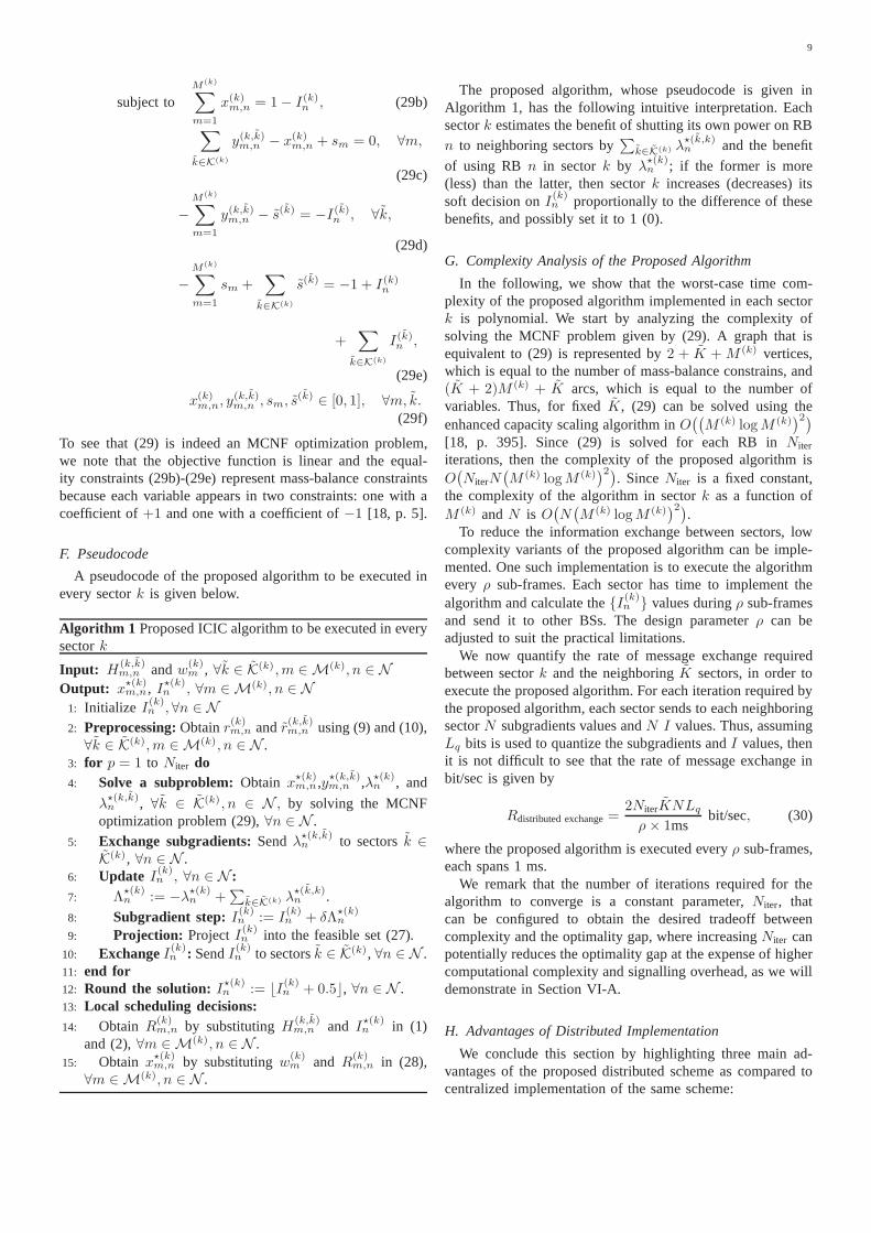
F. Pseudocode

A pseudocode of the proposed algorithm to be executed inevery sectork is given below.

Algorithm 1 Proposed ICIC algorithm to be executed in everysectork

Input: H(k,k)m,n andw(k)

m , ∀k ∈ K(k),m ∈ M(k), n ∈ N

Output: x⋆(k)m,n , I⋆(k)n , ∀m ∈ M(k), n ∈ N

1: Initialize I(k)n , ∀n ∈ N

2: Preprocessing:Obtainr(k)m,n andr(k,k)m,n using (9) and (10),∀k ∈ K(k),m ∈ M(k), n ∈ N .

3: for p = 1 to Niter do4: Solve a subproblem:Obtain x

⋆(k)m,n ,y⋆(k,k)m,n ,λ⋆(k)

n , and

λ⋆(k,k)n , ∀k ∈ K(k), n ∈ N , by solving the MCNF

optimization problem (29),∀n ∈ N .5: Exchange subgradients:Sendλ⋆(k,k)

n to sectorsk ∈K(k), ∀n ∈ N .

6: Update I(k)n , ∀n ∈ N :

7: Λ⋆(k)n := −λ

⋆(k)n +

∑

k∈K(k) λ⋆(k,k)n .

8: Subgradient step:I(k)n := I(k)n + δΛ

⋆(k)n

9: Projection: ProjectI(k)n into the feasible set (27).10: ExchangeI(k)n : SendI(k)n to sectorsk ∈ K(k), ∀n ∈ N .11: end for12: Round the solution: I⋆(k)n := ⌊I

(k)n + 0.5⌋, ∀n ∈ N .

13: Local scheduling decisions:14: Obtain R

(k)m,n by substitutingH(k,k)

m,n and I⋆(k)n in (1)

and (2),∀m ∈ M(k), n ∈ N .15: Obtain x

⋆(k)m,n by substitutingw(k)

m and R(k)m,n in (28),

∀m ∈ M(k), n ∈ N .

The proposed algorithm, whose pseudocode is given inAlgorithm 1, has the following intuitive interpretation. Eachsectork estimates the benefit of shutting its own power on RBn to neighboring sectors by

∑

k∈K(k) λ⋆(k,k)n and the benefit

of using RB n in sectork by λ⋆(k)n ; if the former is more

(less) than the latter, then sectork increases (decreases) itssoft decision onI(k)n proportionally to the difference of thesebenefits, and possibly set it to 1 (0).

G. Complexity Analysis of the Proposed Algorithm

In the following, we show that the worst-case time com-plexity of the proposed algorithm implemented in each sectork is polynomial. We start by analyzing the complexity ofsolving the MCNF problem given by (29). A graph that isequivalent to (29) is represented by2 + K + M (k) vertices,which is equal to the number of mass-balance constrains, and(K + 2)M (k) + K arcs, which is equal to the number ofvariables. Thus, for fixedK, (29) can be solved using theenhanced capacity scaling algorithm inO

((

M (k) logM (k))2)

[18, p. 395]. Since (29) is solved for each RB inNiter

iterations, then the complexity of the proposed algorithm isO(

NiterN(

M (k) logM (k))2)

. SinceNiter is a fixed constant,the complexity of the algorithm in sectork as a function ofM (k) andN is O

(

N(

M (k) logM (k))2)

.To reduce the information exchange between sectors, low

complexity variants of the proposed algorithm can be imple-mented. One such implementation is to execute the algorithmevery ρ sub-frames. Each sector has time to implement thealgorithm and calculate the{I(k)n } values duringρ sub-framesand send it to other BSs. The design parameterρ can beadjusted to suit the practical limitations.

We now quantify the rate of message exchange requiredbetween sectork and the neighboringK sectors, in order toexecute the proposed algorithm. For each iteration required bythe proposed algorithm, each sector sends to each neighboringsectorN subgradients values andN I values. Thus, assumingLq bits is used to quantize the subgradients andI values, thenit is not difficult to see that the rate of message exchange inbit/sec is given by

Rdistributed exchange=2NiterKNLq

ρ× 1msbit/sec, (30)

where the proposed algorithm is executed everyρ sub-frames,each spans 1 ms.

We remark that the number of iterations required for thealgorithm to converge is a constant parameter,Niter, thatcan be configured to obtain the desired tradeoff betweencomplexity and the optimality gap, where increasingNiter canpotentially reduces the optimality gap at the expense of highercomputational complexity and signalling overhead, as we willdemonstrate in Section VI-A.

H. Advantages of Distributed Implementation

We conclude this section by highlighting three main ad-vantages of the proposed distributed scheme as compared tocentralized implementation of the same scheme:

10

I. It does not require a centralized entity to collect thechannel information from all UTs in the network andmake network-wide scheduling decisions. This particularadvantage makes the proposed algorithm applicable tocurrent and emerging standards such as LTE and LTE-advanced, where a centralized entity is not supported.

II. The proposed algorithm can potentially reduce the mes-sage exchange as compared to a centralized implementa-tion. To elaborate, we start by quantifying the rate ofmessage exchange required for centralized implemen-tation between each sectork and a centralized entityand then compare it with the rate of message exchangefor the distributed scheme given in (30). Since eachsector k is required to send to the centralized entityN × M (k)(K + 1) channel coefficients and assumingLq bits is used to quantize the channel coefficients, thenit is not difficult to see that the rate of message exchangefor a centralized implementation in bit/sec is given by

Rcentralized exchange=N ×M (k)(K + 1)Lq

ρ× 1msbit/sec.

(31)Using (30) and (31), the ratio of the rate of messageexchange required by the centralized scheme to the rateof message exchange by the proposed scheme is givenby

Rcentralized exchange

Rdistributed exchange=

M (k)(K + 1)

2(K)Niter. (32)

Thus, as long asNiter <12M

(k)(1 + 1K), then the pro-

posed distributed implementation requires lower rate ofmessage exchange than the centralized implementation.For instance, ifM (k) = 20 UTs, K = 6 interferers, andNiter = 5, then, the proposed scheme requires 2.33 timeslower rate of message exchange than the centralizedimplementation.

III. The amount of computations that is needed to be per-formed in a centralized entity will scale at least linearlywith the number of sectors,K. Thus, scaling the networkwould require to scale also the computational capabil-ities of the centralized entity. However, this is not anissue for the proposed distributed implementation sincethe computations required are distributed among theKsectors and the computations needed by each sector isindependent of the number of sectors in the network.

V. SIMULATION SETUP AND PARAMETERS

The simulation parameters are based on the IMT-AdvancedUrban macro-cell (UMa) scenario [21] which are provided inTable III. Based on the IMT-Advanced guidelines, a hexagonallayout with wrapround is considered with57 hexagonal sectorsand 10 UTs per sector. These sectors are served by19 BSs,each with a tri-sector antenna to serve a 3-sector cell-site.Monte Carlo simulations are carried over1000 sub-framesand averaged over 10 independent drops. In each drop, theaverage received power from all sectors are calculated for eachUT; this involves the calculation of the pathloss, correlatedshadowing, and antenna gains. Variations of the received signal

TABLE IITHE AMC TABLE WHICH IS USED TO DETERMINE THE ACHIEVABLE DATA

RATE ON EACH RB FOR EACH USER BASED ON THESINR. THIS TABLE ISBASED ON THEAMC STRATEGY GIVEN IN [37].

RB SINR Data rate RB SINR Data raterange (dB) per RB (kbit/sec) range (dB) per RB (kbit/sec)

(−∞ -6.1] 0 (5.8, 8.5] 291.6(-6.1, -4.1] 35.3 (8.5, 9.9] 388.4(-4.1, -2.0] 56.4 (9.5, 12.5] 418.3(-2.0, -0.2] 92.4 (12.5, 14.8] 544.3(-0.2, 1.9] 131.4 14.8. 16.1] 648.1(1.9, 3.8] 177.4 (16.1, 17.8] 721.7(3.8, 5.8] 223.1 (17.8,∞) 807.4

TABLE IIISIMULATION PARAMETERS BASED ONIMT-A DVANCED UMA SCENARIO.

Parameter Assumption

Number of sectors 57 (wraparound)Number of UTs per sector 10

Inter-site distance 500 mBS height 25 m

Min. dist. between a UT and a BS 25 mUT speed 30 km/h

Bandwidth (downlink) 10 MHzSub-carrier spacing 15 KHz

Number of RBs (N ) 50OFDM symbol duration 66.67 µs

Number of sub-carriers per RB 12Number of OFDM symbols per RB 7

Number of drops 10Number of sub-frames per drop 1000

Noise power per RB (PN ) -114.45 dBmCarrier frequency 2.0 GHz

Total BS transmit power 46 dBmPath loss and shadowing Based on UMa scenario [21]Averaging window (tc) 100

BS antenna gain (boresight) 17 dBiUser antenna gain 0 dBi

Feeder loss 2 dBChannel estimation delay 4 sub-framesSINR estimation margin 6 dB

BS antenna tilt(φt) 12◦ [38]

BS horizontal antenna pattern A(θ) = −min[

12( θ70◦

)2, 20 dB]

BS elevation antenna pattern Ae(φ) = −min[

12(φ−φt

15◦)2, 20 dB

]

BS combined antenna pattern −min [− (A(θ) + Ae(φ)) , 20 dB] [21]Small-scale fading model IMT-Advanced channel model [36]

Traffic model Full buffer

power due to small-scale fading within each RB is negligibleand thus, the channels are assumed fixed over each RB. Forother RBs, the channels assume different values depending onthe time-frequency correlation of the IMT-Advanced modelfor the UMa scenario [36]. We use the AMC strategy givenin Table II [37]. Channel-aware scheduling and ICIC aredone afterwards, on a sub-frame by sub-frame basis. Afterscheduling the last sub-frame, the time-average throughput foreach user is calculated. Then, another drop commences and theprocess repeats. Finally, time-averaged users throughputfromall drops are saved for further processing and plotting. Furtherdetails of the simulation procedure are given in [21, Section7]. The simulator is validated with the UMa simulation resultsprovided in [38].

A. Importance of Accurate Simulation

Although explaining how to do accurate simulations is notthe main purpose of this paper, we nevertheless highlightan aspect in the simulation that has important effect on

11

assessing the performance of ICIC schemes. In particular, wedemonstrate that the way UTs are associated to sectors has asignificant impact on the simulation results. In the following,we explain three association strategies, namely, widebandSINR-based, wideband SINR-based (excluding shadowing),and geographical-based association. Wideband SINR is de-fined as the ratio of the average power received from theserving sector to the sum of the average power received fromall other sectors and the noise power at the UT (i.e., smallscale fading is not included in the calculation of the widebandSINR). In wideband SINR-based association, each UT isassociated with the antenna sector to which it has the highestwideband SINR. This association strategy resembles reality,provides the most favorable results, and it is widely used byevaluation groups. A consequence of this strategy is that thecoverage region of each sector is not hexagonal and it changesfrom drop to drop due to the different shadowing realizations.Another consequence is that a UT may not be associatedto the closest sector antenna as it may experience heavyshadowing to that sector antenna. A more convenient way ofdoing simulation is to exclude shadowing in the calculationof the wideband SINR which leads to fixed coverage regionsfor each sector in all drops. Due to the directional antennapatterns, the coverage regions of each sector is not hexagonal.In geographical-based association, a UT is associated to aparticular sector antenna if it resides inside the hexagonal areaof that sector. In this strategy, the coverage region of eachsector is hexagonal.

In Fig. 2, we plot the CDF of the wideband SINR usingthe three association strategies for reuse-1. For validationpurposes, we also include the average CDF results produced byseven WINNER+ partners using different simulation tools forUMa scenario [38]. It is clear from the figure that widebandSINR-based association strategy produces a CDF that agreevery well with the calibrated results; however, the other twoassociation strategies produce a heavy tail which would impactthe throughput of the users at the cell edge. The heavytail is a direct consequence of associating UTs to sectorsin a suboptimal manner. As a result, these two associationstrategies may not be suitable for assessing the performanceof ICIC schemes as they tend to exaggerate the gains achievedfor UTs at the cell-edge. This is the case because the cell-edge user throughput for reuse-1 for these two associationstrategies is very low. This makes any improvement in cell-edge user throughput to be large as compared to the verylow values of reuse-1. Consequently, we use wideband SINR-based association strategy to assess the performance of ICICschemes.

We conclude this section by highlighting the main motiva-tions for performing SINR validation in system simulations:

1) System simulators are complex in nature which makethem error-prone. As a result, careful verification of thesimulation results is imperative.

2) Validation of the simulation makes it easy for otherresearchers to compare the performance of our schemeswith other schemes in a widely-accepted scenario suchas the UMa scenario specified by IMT-advanced.

3) As we observed in Fig. 2, the gains of ICIC schemes may

be exaggerated if the simulation assumptions, such as theUT-BS association strategy, does not resemble reality.Validation of the SINR distribution is a good way toverify the validity of the simulation assumptions.

−25 −20 −15 −10 −5 0 5 10 150

0.1

0.2

0.3

0.4

0.5

0.6

0.7

0.8

0.9

1

PSfrag replacements

dB

Pro

bab

ility

(Wid

eban

dS

INR<

Ab

scis

sa) Wideband SINR-based

Wideband SINR-based(excluding shadowing)Geographically-basedReference results (WINNER+)

Fig. 2. CDF of the wideband SINR for different association strategies.Reference results (WINNER+) refers to the average CDF results produced byseven WINNER+ partners [38].

B. Baseline Schemes

In this paper, the followings are used as baseline schemes:reuse-1, reuse-3, partial frequency reuse (PFR) [5], dynamicFFR [9], and optimum FFR [39]. While reuse-1, reuse-3,and PFR are static schemes, dynamic and optimum FFR areimplemented as dynamic schemes.

In PFR, RBs are divided such as 30 RBs (inner band) areused in all sectors (reuse-1) while 20 RBs (outer band) areshared among sites in a classical reuse-3 pattern. More detailsabout this algorithm can be found in [5].

While dynamic FFR and optimum FFR were designedto maximize the sum-rate, they can be easily modified toaccommodate maximizing weighted sum-rates, and they workwith differentiable and non-differentiable AMC functions,which make them good baseline schemes to be compared withthe proposed scheme. For fair comparison, we convert theconstraint on instantaneous minimum rate (used in dynamicand optimum FFR) to a constraint on average minimumrate, which can be implemented by updating the weights inevery sub-frame according to the procedure given in [31]. Wefinally remark that both dynamic FFR and optimum FFR arecentralized schemes.

In dynamic FFR, a centralized controller is used to deter-mine which RBs belong to inner band (in reuse-1 pattern) andwhich RBs belong to outer bands (in reuse-3 pattern). Thedecision is made to maximize the total utility, assuming eachRB is used by all the users in the region where this RB canbe used, and summed for all the sectors. This assumption iscritical to the development of the algorithm. Then, scheduling

12

is done locally by each BS. More details about this algorithmcan be found in [9].

In optimum FFR, the number of RBs used in inner andouter bands, and the reuse factor of the outer band aredetermined optimally using a centralized controller, withoutconsidering channel fading. Without channel fading, all RBsseen by a particular user have the same SINR. This makes theoptimization problem tractable. However, if channel fading isconsidered, then the computational complexity for optimumFFR is exponential. More details about this algorithm can befound in [39].

It is common for FFR schemes (e.g., PFR and optimumFFR) to divide users into two classes: inner (cell-center) usersand outer (cell-edge) users, based on SINR or distance fromBS. Inner users are restricted to use inner band while outerusers are restricted to use outer band. We found such restrictiondegrades the performance of FFR and as such, this restrictionis removed to realize the full potential of FFR schemes. Thisrestriction is already removed from dynamic FFR [9] for thesame reason.

VI. SIMULATION AND ANALYTICAL RESULTS

A. Optimality Gaps

To develop an efficient algorithm to solve the difficult opti-mization problem given by (13) in a distributed manner, twosources of sub-optimality were introduced, namely, relaxingthe integer constraints and solving the master optimizationproblem in finite iterations. To understand the effect of thesesources of sub-optimality, we present in Fig. 3 the meanoptimality gap (21), the 5th percentile, and 95th percentileof the distribution of the optimality gap obtained from simu-lating 22,000 instances of optimization problems for differentnumbers of UTs and four IMT-Advanced scenarios, namely,UMa, Urban micro-cell (UMi), Rural macro-cell (RMa), andSuburban macro-cell (SMa) scenarios [1]. In the first sub-frame, a random initial point is used. In the subsequent sub-frames, the optimal solution of the previous frame is used asan initial point. As it can be seen from this figure, the proposedalgorithm converges fast to low optimality gaps; in particular,executing the algorithm in 5 iterations provided less than 1.5%mean optimality gap. As a result, the number of iterations,Niter, is chosen to beNiter = 5 throughout the paper.

Fig. 3 illustrates that our algorithm can solve the boundoptimization problem (13), which is suitable in dominant inter-ference environment, in a near-optimum manner, as expectedfrom Proposition 1. A natural question to ask is how differentis the optimal value obtained by solving the bound optimiza-tion as compared to the optimal value obtained by solvingthe original strongly NP-hard problem (7) using exhaustivesearch? Due to the exponential computational complexity ofexhaustive search, simulating a system of 57 sectors is notfeasible. As a result, we only show the optimality gap fora system of 12 sectors in Table IV, for proportional-fairscheduling, i.e.,α = 1. As we can see, the proposed schemecan achieve, on average, about 96% of the optimum valueachieved using exhaustive search, if it is executed once (5iterations). One can also reduce the optimality gap furtherby

TABLE IVMEAN AND STANDARD DEVIATION OF THE OPTIMALITY GAP (%)

COMPARED TO THE OPTIMAL VALUE OF THE ORIGINAL PROBLEM(7)

Number of runs Mean (%) Standard deviation (%)1 3.8 1.72 2.4 0.8

executing the algorithm more than once. That is, after findingthe optimum{I(k)n } in one run, the algorithm setsH(k,k)

m,n = 0,

∀m,n, k, k|I(k)n = 1, and executes the algorithm again. In

this case, one can achieve about 97.6% of the optimum valueachieved using exhaustive search, i.e., an incremental gain, atthe expense of more computational complexity. This suggeststhat the bound optimization is indeed a good method to achievenear-optimality and shows that most of the gain is alreadycaptured by executing the algorithm only once.

0 2 4 6 8 100

5

10

15

20

25

30

35

40

45

50

PSfrag replacements

Number of Iterations

Op

timal

ityG

ap(%

)

95th percentile

5th percentile

Mean

Fig. 3. Optimality gap (%) as a function of the number of iterations.

B. Comparing the Performance of the Proposed Scheme withthe Baseline Schemes

In this section, we compare the performance of the proposedscheme with the baseline schemes presented in Section V-B.In Fig. 4, we show the CDF of the normalized time-averageUT throughput for all schemes. Normalization is performedby dividing the user throughput over the total downlinkbandwidth, which is10 MHz. In all schemes,α-fair scheduleris used with fairness exponent ofα = 2 (cf. Section III).To facilitate the comparison, we define the normalized cell-edge and cell-center user throughputs as the5th and the95th

percentiles of the normalized user throughputs, respectively.It is clear from the figure that reuse-1 has the worst cell-edge performance (0.0323 bit/sec/Hz) as compared to the otherthree schemes, due to the excessive interference experiencedat the cell-edge. Reuse-3, PFR, dynamic FFR, optimum FFR,and the proposed scheme achieve normalized cell-edge userthroughputs of 0.0391, 0.0417, 0.0412, 0.0435, and 0.0430

13

bit/sec/Hz, respectively. However, reuse-3, PFR, dynamicFFR,and optimum FFR improve the cell-edge performance at theexpense of reducing the overall throughput, especially forUTs close to the cell-center. For example, the95th percentileachieved by reuse-3, PFR, dynamic FFR, and optimum FFRare 0.108, 0.136, 0.107, and 0.125 bit/sec/Hz, respectively, ascompared to 0.156 and 0.154 bit/sec/Hz achieved by reuse-1 and the proposed scheme, respectively. Interestingly, theproposed scheme combines the advantages of all schemes, asit provides high cell-edge and cell-center throughputs simulta-neously. In addition to the improvement in cell-center and cell-edge throughputs, the proposed scheme also outperforms theother schemes in terms of the normalized median throughput(50th percentile). Indeed, the gain achieved by the proposedscheme increases for higher fairness exponent,α, or higherRmin, as we will see shortly.

0 0.05 0.1 0.15 0.20

0.1

0.2

0.3

0.4

0.5

0.6

0.7

0.8

0.9

1

0 0.02 0.040

0.05

Zoomed

PSfrag replacements

Pro

bab

ility

(No

rmal

ized

use

rth

rou

gh

pu

t<

Ab

scis

sa)

bit/sec/Hz

Reuse-1Reuse-3PFRDynamic FFROptimum FFRProposed

Fig. 4. CDF of the normalized user throughput of all UTs in thenetworkfor UMa scenario,α = 2 and Rmin = 0.

To further examine the performance of the differentschemes, we show in Fig. 5 the normalized cell-edge userthroughput and the normalized aggregate sector throughputforall schemes and for different minimum average rate require-mentsRmin, assuming proportional-fair scheduler, i.e.,α = 1.As expected, the general trend for all schemes is that asRmin

increases, the sector throughput decreases and the cell-edgeuser throughput increases. For highRmin, we observe thatreuse-3, PFR, optimum FFR, dynamic FFR, and the proposedscheme have significantly higher cell-edge throughput thanreuse-1. On the other hand, for smallRmin it is clear thatreuse-3, PFR, dynamic FFR, and optimum FFR incur signif-icant loss in the aggregate sector throughput as compared toreuse-1. Interestingly, the proposed scheme performs verywellin both the cell-edge and the sector throughput as compared toall other schemes for all values ofRmin. We also plot similartradeoff curves in Fig. 6 by varying the fairness exponentαand fixing Rmin = 0, similar to [40]. Again, the proposedscheme outperforms other schemes in both the cell-edge and

the aggregate sector throughput.

0.65 0.7 0.75 0.8 0.85 0.9 0.95 1 1.05 1.10.02

0.025

0.03

0.035

0.04

0.045

0.05

0.055

0.06

0.065

00.02

0.03

0.04

0.050.06

00.02

0.03

0.040.050.06

00.020.03

0.04

0

0.02

0.03

0.04

0.05

0.06

00.02

0.03

0.04

0.050.06

00.02

0.03

0.040.05

0.06

00.020.03

0.04

0

0.02

0.03

0.04

0.05

0.06

00.02

0.03

0.04

0.050.06

00.02

0.03

0.040.05

0.06

00.020.03

0.04

0

0.02

0.03

0.04

0.05

0.060.07

0.07

0.07

0.07 0.06

0.05

PSfrag replacements

Normalized aggregate sector throughput (bit/sec/Hz)

No

rmal

ized

cell-

edg

eth

rou

gh

pu

t(b

it/se

c/H

z) Reuse-1Reuse-3PFRDynamic FFROptimum FFRProposed

Fig. 5. Normalized cell-edge throughput versus normalizedaggregate sectorthroughput for different schemes, forα = 1 and Rmin ∈ {0, 0.02, 0.03,0.04, 0.05, 0.06, 0.07}.

0.7 0.8 0.9 1 1.1 1.2 1.3 1.4 1.5 1.60

0.01

0.02

0.03

0.04

0.05

0.06

0.5

1

4

0

0.25

0.5

0.75

1

2 3

4

0

0.25

0.5

0.75

1

2 3

0

0.25

0.5

0.75

1

2

3

45

3

1

2

54

5

5

PSfrag replacements

Normalized aggregate sector throughput (bit/sec/Hz)

No

rmal

ized

cell-

edg

eu

ser

thro

ug

hp

ut

(bit/

sec/

Hz)

Reuse-1

Reuse-3PFR

Dynamic FFR

Optimum FFRProposed

Fig. 6. Normalized cell-edge throughput versus normalizedaggregate sectorthroughput for different schemes, forRmin = 0 and α ∈ {0, 0.25, 0.50,0.75, 1, 2, 3, 4, 5}.

In Fig.s 7 and 8, we take a closer look at the gains achievedby the different schemes as compared to reuse-1. In Fig. 7,we plot the gains in cell-edge throughput achieved for a givenaggregate sector throughput. The gain in cell-edge throughputfor a particular scheme for a given sector throughputx isgiven by Gainscheme(x) =

CellEdgescheme(x)−CellEdgereuse1(x)CellEdgereuse1(x)

· 100%,where CellEdgescheme(x) is the cell-edge throughput achievedby a particular scheme at sector throughputx, which canbe obtained from the tradeoff curves given in Fig. 5. Fora wide range of aggregate sector throughput, the proposedscheme achieves large gains (50% to 60%). Dynamic FFR,

14

optimum FFR, and the proposed scheme lose some of thegain if it is executed every 10 sub-frames (as expected for anydynamic scheme); however, the gains for the proposed schemeare consistently better than the other schemes. Similarly,weplot the gains in aggregate sector throughput for a given cell-edge throughput in Fig. 8. The proposed scheme achievesconsistently higher gains in aggregate sector throughput thanthe other schemes, especially for high cell-edge throughput.

0.7 0.75 0.8 0.85 0.9 0.95 1 1.05−30

−20

−10

0

10

20

30

40

50

60

PSfrag replacements

Normalized aggregate sector throughput (bit/sec/Hz)

Gai

n(%

)in

cell-

edg

eu

ser

thro

ug

hp

ut

(ρ = 10 sub-frames)

(ρ = 10 sub-frames)

(ρ = 10 sub-frames)

Reuse-1

Reuse-3PFR

Dynamic FFRDynamic FFR

Optimum FFROptimum FFR

ProposedProposed

Fig. 7. Gain (%) in cell-edge throughput versus aggregate sector throughput,as compared to reuse-1.

0.028 0.03 0.032 0.034 0.036 0.038 0.04−20

−10

0

10

20

30

40

50

PSfrag replacements

Normalized cell-edge user throughput (bit/sec/Hz)

Gai

n(%

)in

agg

reg

ate

sect

or

thro

ug

hp

ut

Reuse-1

Reuse-3PFRDynamic FFR

Dynamic FFR (ρ = 10 sub-frames)Optimum FFR

Optimum FFR (ρ = 10 sub-frames)Proposed

Proposed (ρ = 10 sub-frames)

Fig. 8. Gain (%) in sector throughput versus cell-edge throughput, ascompared to reuse-1.

In Fig. 9, we plot the outage probability, which is definedas the probability of having the average UT throughput lessthanRmin for different schemes. It is clear from the figure thatthe proposed scheme achieves much lower outage probabilityas compared to other schemes. For example, atRmin = 0.05bits/sec/Hz, the proposed scheme has an outage probabilitythat is at least 3.5 times less than those for PFR and optimumFFR, and at least 6 times less than those for reuse-1, reuse-3,and dynamic FFR.

PSfrag replacements

Pro

bab

ility

(No

rmal

ized

use

rth

rou

gh

pu

t<

Rmin

)

Rmin (bit/sec/Hz)

Reuse-1

Reuse-3PFR

Dynamic FFR

Optimum FFR

Proposed

0.05

0.01

0.15

0.20

0.25

0.30

0.35

0.40

00 0.01 0.02 0.03 0.04 0.05 0.06

Fig. 9. Outage probability versusRmin, which is defined as the probabilitythat the average UT throughput less thanRmin.

TABLE VCOMPARISON BETWEEN THE PROPOSED DISTRIBUTED SCHEME, DYNAMIC

FFR,AND OPTIMUM FFR, IN TERMS OF COMPUTATIONAL COMPLEXITY

AND RATE OF MESSAGE EXCHANGE REQUIRED

Scheme Computational complexity Rate of messageexchange required

Centralized entity Sectork for sectork (bit/sec)

Proposed Scheme None O(

N(

M (k) logM (k))2) 2NiterKNLq

ρ×1ms

Dynamic FFR [9] O(

N(N − 1)K) O(

NM (k))2NM(k)Lq

ρ×1ms

Optimum FFR [39] O(

N2K∑

k=1

M (k)) O(

NM (k))M(k)Lq

ρ×1ms

C. Comparing the Complexity of the Proposed Scheme withthe Baseline Schemes

By analyzing the dynamic FFR algorithm in [9] and theoptimum FFR algorithm in [39], we obtained the computa-tional complexity and the rate of message exchange requiredto execute both algorithms. Due to space limitation, we onlysummarize the final result in Table V. In terms of compu-tational complexity, it can be seen from Table V that theproposed algorithm scales better (worse) than dynamic andoptimum FFR asN orK (M (k)) increases. In terms of the rateof message exchange, the proposed scheme scales better thandynamic and optimum FFR asM (k) increases, while optimumFFR scales best asN increases.

D. Statistics of the Average Number of Blanked RBs

In Fig. 10, we plot the probability mass function of theaverage number of blanked RBs per sector for differentfairness exponents. The proposed scheme has the flexibilityto change the distribution of the blanked resources accordingto the desired fairness level. Asα increases, cell-edge usersbecome more important and thus more resources need tobe blanked, and vice versa. The figure shows also that theproposed scheme acts as reuse-1 (no blanking) and reuse-3(2/3 of RBs are blanking) with very small probabilities.

15

0 10 20 30 40 500

0.02

0.04

0.06

0.08

0.1

0.12

0.14

PSfrag replacements

Pro

bab

ility

(Nu

mb

ero

fb

lan

ked

RB

s=

Ab

scis

sa)

α = 1α = 4α = 10

Reuse-1 Reuse-3PFR

Fig. 10. Probability mass function of the average number of blanked RBsper sector (the total number of RBs is 50).

VII. C ONCLUSIONS

In this paper, we tackled the problem of distributed multi-cell resource allocations with blanking where the objective isto maximize the weighted sum-rate. This problem is knownto be strongly NP-hard problem; nevertheless, we demon-strated that this problem can be tightly relaxed to a linearprogramming problem in a dominant interference environment,in which for each user the received power from each interfereris significantly greater than the aggregate received powerfrom all other weaker interferers. Using linear relaxation,we proposed a polynomial-time distributed algorithm that isnot only guaranteed to be tight for dominant interferenceenvironment, but which also computes an upper bound on theoptimality gap. The proposed scheme is developed using theprimal-decomposition method, which is utilized to decomposethe problem into a master problem and multiple subproblems.The master problem is solved iteratively using the projected-subgradient method. We reveal that each subproblem has anetwork flow structure which makes it amenable to powerfulMCNF algorithms and thus results in significant reduction inthe computational complexity. Simulation results show that theproposed scheme achieves high gain in aggregate throughout,cell-edge throughput, and outage probability, as comparedtoreuse-1, reuse-3, partial frequency reuse, dynamic fractionalfrequency reuse, and optimum fractional frequency reuse. Aninteresting extension to this work is to use the decompositionalgorithms proposed in [41] to devise distributed ICIC algo-rithms.

ACKNOWLEDGMENT

The authors would like to express their gratitude to Dr. HoTing Cheng and Dr. Zhijun Chao from Huawei TechnologiesCanada, and Dr. Ramy Gohary from Carleton University, fortheir helpful comments and suggestions.

APPENDIX AON THE TIGHTNESS OF THE BOUND GIVEN IN(8)

In this Appendix, we show that the SINR bound givenby (8) is tight in the sense if the bound is increased by∆, then the actual SINR will increase by at least∆. Let

k⋆ = arg maxk∈K(k)

I(k)n H

(k,k)m,n , then the exact SINR expression

given by (1) can be written as

Γ(k)m,n =

PCH(k,k)m,n

PC

(

∑

k 6=k

H(k,k)m,n −Ik⋆

n H(k,k⋆)m,n −

∑

k 6=k,k 6=k⋆

I(k)n H

(k,k)m,n

)

+PN

,

=PCH(k,k)

m,n

PC

(

∑

k 6=k

H(k,k)m,n −Ik⋆

n H(k,k⋆)m,n

)

+PN

×

1 +

PC

∑

k 6=k,k 6=k⋆

I(k)n H(k,k)

m,n

PC

∑

k 6=k

(

1−I(k)n

)

H(k,k)m,n +PN

≥PCH(k,k)

m,n

PC

(

∑

k 6=k

H(k,k)m,n −Ik⋆

n H(k,k⋆)m,n

)

+PN

,

(33)where the right-hand side of the inequality is the boundgiven by (8). From the previous expression, if the boundis increased by∆, then Γ

(k)m,n will increase by∆ ×

(

1 +

PC

K∑

k=1,k 6=k,k 6=k⋆

I(k)n H(k,k)

m,n

PC

K∑

k=1,k 6=k

(

1−I(k)n

)

H(k,k)m,n +PN

)

, i.e.,Γ(k)m,n will increase by at

least∆.

APPENDIX BPROOF OFLEMMA 1

We proceed by proving thatC ⊆ C′ andC′ ⊆ C. To provethat C ⊆ C′, we assume thaty(k,k)m,n ∈ C and deduce that

y(k,k)m,n ∈ C′. Since

∑

k∈K(k) y(k,k)m,n ≤ 1 andy(k,k)m,n ≤ x

(k)m,n, then

∑

k∈K(k) y(k,k)m,n ≤ x

(k)m,n. Moreover, sincey(k,k)m,n ≤ x

(k)m,n, then

∑M(k)

m=1 y(k,k)m,n ≤

∑M(k)

m=1 x(k)m,n ≤ 1. Since

∑M(k)

m=1 y(k,k)m,n ≤ 1,

y(k,k)m,n ≤ I

(k)n , andy(k,k)m,n ∈ {0, 1}, then

∑M(k)

m=1 y(k,k)m,n ≤ I

(k)n .

Consequently,y(k,k)m,n ∈ C′, which means thatC ⊆ C′.

Similarly, to show thatC′ ⊆ C, we assume thaty(k,k)m,n ∈ C′

and deduce thaty(k,k)m,n ∈ C. Since∑

k∈K(k) y(k,k)m,n ≤ x

(k)m,n

and x(k)m,n, y

(k,k)m,n ∈ {0, 1}, then y

(k,k)m,n ≤ x

(k)m,n. Moreover,

since∑M(k)

m=1 y(k,k)m,n ≤ I

(k)n and I

(k)n , y

(k,k)m,n ∈ {0, 1}, then

∑M(k)

m=1 y(k,k)m,n ≤ 1 which means thaty(k,k)m,n ≤ I

(k)n . Hence,

y(k,k)m,n ∈ C which means thatC′ ⊆ C.

APPENDIX CPROOF OFPROPOSITION1

We start by categorizing the constraints of the relaxed ver-sion of (18) into two groups: non-bounding constraints, whichare given by (18b), (18c), and (18d), and bounding constraints,which are given by (19) (relaxed version of (18e)). It iseasy to see that the number of variables that assume optimalbinary values is equal to the number of bounding inequalityconstraints that are active at the optimal, i.e., inequalities thatare satisfied with equalities at the optimal.

16

We now note that the optimal solution of a linear programlies on one or more vertices. For a linear program withNvar variables, a vertex is characterized byNvar equalitiesor active inequalities. LetN⋆

non−bounding denote the numberof non-bounding equality or active inequality constraintsatthe optimum, and letN⋆

bounding denote the number of activebounding inequality constraints at the optimum. Hence, wecan write the following:

Nvar = N⋆bounding +N⋆

non−bounding

⇒ N⋆bounding = Nvar −N⋆

non−bounding

⇒ N⋆bounding ≥ Nvar − sup(N⋆

non−bounding)

= (K + 1)∑K

k=1 M(k) +K

−(K +∑K

k=1(M(k) + K))

=∑K

k=1 K(M (k) − 1),

(34)

where the supremum is found by assuming that all non-bounding constraints are active. Thus, the percentage of opti-mal variables of the relaxed version of (18) that assume binaryvalues can be bounded as

Pbinary ≥K∑K

k=1(M(k)−1)

(K+1)∑

Kk=1 M(k)+K

· 100%

= K(M−1)

(K+1)M+1· 100%,

(35)

whereM is the average number of UTs per sector, i.e.,M =1K

∑K

k=1 M(k).

REFERENCES

[1] A. Bin Sediq, R. Schoenen, H. Yanikomeroglu, G. Senarath, andZ. Chao, “A novel distributed inter-cell interference coordination schemebased on projected subgradient and network flow optimizations,” in Proc.IEEE Int. Symp. on Pers., Indoor and Mobile Radio Commun. (PIMRC),Toronto, Canada, Sep. 2011.

[2] T. S. Rappaport,Wireless Communications: Principles and Practice.Prentice-Hall, 1996.

[3] M. Rahman and H. Yanikomeroglu, “Enhancing cell-edge performance:A downlink dynamic interference avoidance scheme with inter-cellcoordination,”IEEE Trans. Wireless Commun., vol. 9, no. 4, pp. 1414–1425, Apr. 2010.

[4] 3GPP Project Doc. R1-050 507, “Soft frequency reuse scheme forUTRAN LTE,” Tech. Rep., May 2005.

[5] M. Sternad, T. Ottosson, A. Ahlen, and A. Svensson, “Attaining bothcoverage and high spectral efficiency with adaptive OFDM downlinks,”in Proc. IEEE Veh. Tech. Conf. (VTC-Fall), Orlando, Florida, Oct. 2003.

[6] Y. Xiang, J. Luo, and C. Hartmann, “Inter-cell interference mitigationthrough flexible resource reuse in OFDMA based communication,” inProc. 13th European Wireless Conf., Paris, France, Apr. 2007.

[7] A. Simonsson, “Frequency reuse and intercell interference co-ordinationin E-UTRA,” in Proc. IEEE Veh. Tech. Conf. (VTC-Spring), Dublin,Ireland, Apr. 2007.

[8] 3GPP Project Doc. R1-072 762, “Further discussion on adaptive frac-tional frequency reuse,” Tech. Rep., Jun. 2007.

[9] S. H. Ali and V. C. M. Leung, “Dynamic frequency allocation infractional frequency reused OFDMA networks,”IEEE Trans. WirelessCommun., vol. 8, no. 12, pp. 4286–4295, Aug. 2009.

[10] X. Zhang, C. He, L. Jiang, and J. Xu, “Inter-cell interference coordi-nation based on softer frequency reuse in OFDMA cellular systems,”in Proc. Int. Conf. on Neural Net. and Signal Process. (ICNNSP),Zhenjiang, China, Jun. 2008.

[11] X. Mao, A. Maaref, and K. H. Teo, “Adaptive soft frequency reusefor inter-cell interference coordination in SC-FDMA based3GPP LTEuplinks,” in Proc. IEEE Glob. Commun. Conf. (Globecom), New Orleas,LA, Dec. 2008.

[12] A. Stolyar and H. Viswanathan, “Self-organizing dynamic fractionalfrequency reuse for best-effort traffic through distributed inter-cellcoordination,” inProc. IEEE Int. Conf. Comp. Commun. (INFOCOM),Rio de Janeiro, Brazil, Apr. 2009.

[13] D. Bultmann, T. Andre, and R. Schoenen, “Analysis of 3GPP LTE-Advanced cell spectral efficiency,” inProc. IEEE Int. Symp. on Pers.,Indoor and Mobile Radio Commun. (PIMRC), Istanbul, Turkey, Sep.2010.

[14] G. Li and H. Liu, “Downlink radio resource allocation for multi-cellOFDMA system,” IEEE Trans. Wireless Commun., vol. 5, no. 12, pp.3451 –3459, Dec. 2006.

[15] R. Y. Chang, Z. Tao, J. Zhang, and C. C. J. Kuo, “MulticellOFDMAdownlink resource allocation using a graphic framework,”IEEE Trans.Veh. Technol., vol. 58, no. 12, pp. 3494–3507, Sep. 2009.

[16] J. Ellenbeck, C. Hartmann, and L. Berlemann, “Decentralized inter-cellinterference coordination by autonomous spectral reuse decisions,” inProc. 14th European Wireless Conf., Prague, Czech Republic, Jun. 2008.

[17] Z.-Q. T. Luo and S. Zhang, “Dynamic spectrum management: Complex-ity and duality,” IEEE J. Select. Topics Signal Processing, vol. 2, no. 1,pp. 57–73, Feb. 2008.

[18] R. Ahuja, T. Magnanti, and J. Orlin,Network Flows: Theory, Algorithms,and Applications. Prentice Hall, 1993.

[19] M. Tao and Y. Liu, “A network flow approach to throughput maximiza-tion in cooperative OFDMA networks,”IEEE Trans. Wireless Commun.,vol. 12, no. 3, pp. 1138–1148, Mar. 2013.

[20] A. N. Zaki and A. O. Fapojuwo, “Optimal and efficient graph-basedresource allocation algorithms for multiservice frame-based OFDMAnetworks,”IEEE Trans. Mobile Comput., vol. 10, no. 8, pp. 1175–1186,Aug. 2011.

[21] ITU, Report ITU-R M.2135-1, “Guidelines for evaluation of radiointerface technologies for IMT-Advanced,” ITU, Tech. Rep., Dec. 2009.[Online]. Available: http://www.itu.int/pub/R-REP-M.2135-1-2009.

[22] H. Kushner and P. Whiting, “Convergence of proportional-fair sharingalgorithms under general conditions,”IEEE Trans. Wireless Commun.,vol. 3, no. 4, pp. 1250–1259, Jul. 2004.

[23] A. L. Stolyar, “On the asymptotic optimality of the gradient schedulingalgorithm for multiuser throughput allocation,”Oper. Res., vol. 53, no. 1,pp. 12–25, Jan. 2005.

[24] G. Song and Y. Li, “Cross-layer optimization for OFDM wirelessnetworks—part II: Algorithm development,”IEEE Trans. Wireless Com-mun., vol. 4, no. 2, pp. 625–634, Mar. 2005.

[25] J. Mo and J. Walrand, “Fair end-to-end window-based congestioncontrol,” IEEE/ACM Trans. Netw., vol. 8, no. 5, pp. 556–567, Oct. 2000.

[26] T. Lan, D. Kao, M. Chiang, and A. Sabharwal, “An axiomatic theory offairness in network resource allocation,” inProc. IEEE Int. Conf. Comp.Commun. (INFOCOM), San Diego, California, Mar. 2010.

[27] F. P. Kelly, A. K. Maulloo, and D. K. H. Tan, “Rate controlforcommunication networks: Shadow prices, proportional fairness andstability,” J. Oper. Res. Soc., vol. 49, no. 3, pp. 237–252, 1998.

[28] P. Viswanath, D. Tse, and R. Laroia, “Opportunistic beamforming usingdumb antennas,”IEEE Trans. Inf. Theory, vol. 48, no. 6, pp. 1277 –1294,Jun. 2002.

[29] A. Bin Sediq, R. H. Gohary, R. Schoenen, and H. Yanikomeroglu,“Optimal tradeoff between sum-rate efficiency and Jain’s fairness indexin resource allocation,”IEEE Trans. Wireless Commun., vol. 12, no. 7,pp. 3496–3509, Jul. 2013.

[30] H. T. Cheng and W. Zhuang, “An optimization framework for balancingthroughput and fairness in wireless networks with QoS support,” IEEETrans. Wireless Commun., vol. 7, no. 2, pp. 584–593, Feb. 2008.

[31] M. Andrews, L. Qian, and A. Stolyar, “Optimal utility based multi-userthroughput allocation subject to throughput constraints,” in Proc. IEEEInt. Conf. Comp. Commun. (INFOCOM), Miami, Florida, Mar. 2005.

[32] D. P. Bertsekas,Nonlinear Programming, 2nd ed. Athena Scientific,2008.

[33] S. Boyd, L. Xiao, A. Mutapcic, and J. Mattingley, “Noteson decom-position methods,” Lecture notes for EE364B, Stanford University, Oct.2003.

[34] S. Boyd and A. Mutapcic, “Subgradient methods,” Lecture notes forEE364b, Stanford University, Oct. 2003.

[35] S. Boyd, “Subgradients,” Lecture notes for EE364b, Stanford University,Apr. 2011.

[36] J. Nystrom, “Software implementation of IMT.Eval channel model,”CELTIC/CP5-026 Project WINNER+ Doc. 5D/478-E, Tech. Rep.,Jul.2009. [Online]. Available: http://www.itu.int/oth/R0A06000022/en.

[37] R. Schoenen and C. Teijeiro, “System level performanceevaluation ofLTE with MIMO and relays in reuse-1 IMT-Advanced scenarios,” inProc. IEEE WiCom, Chengdu, China, Sep. 2010.

[38] “Calibration for IMT-Advanced evaluations,” CELTIC/CP5-026Project WINNER+, Tech. Rep., May 2010. [Online]. Available:http://projects.celtic-initiative.org/winner+/WINNER+EvaluationGroup.html.

17

[39] M. Assaad, “Optimal fractional frequency reuse (FFR) in multicellularOFDMA system,” inProc. IEEE Veh. Tech. Conf. (VTC-Fall), MarinaBay, Singapore, Sep. 2008.

[40] R. Schoenen, A. Bin Sediq, H. Yanikomeroglu, G. Senarath, andZ. Chao, “Fairness analysis in cellular networks using stochastic Petrinets,” in Proc. IEEE Int. Symp. on Pers., Indoor and Mobile RadioCommun. (PIMRC), Toronto, Canada, Sep. 2011.

[41] G. Scutari, F. Facchinei, P. Song, D. P. Palomar, and J.-S. Pang,“Decomposition by partial linearization: Parallel optimization of multi-agent systems,”IEEE Trans. Signal Process., vol. 62, no. 3, pp. 641–656,Feb. 2014.

PLACEPHOTOHERE

Akram Bin Sediq (S’04) received the B. Sc. degreein electrical engineering (summa cum laude) in 2006from the American University of Sharjah, UnitedArab Emirates, and the M.A.Sc. degree in electri-cal engineering and the Ph.D. degree in electricaland computer engineering from Carleton University,Ottawa, Canada, in 2008 and 2013, respectively. InWinter 2012, Dr. Bin Sediq was a course instructorat the Department of Systems and Computer Engi-neering at Carleton University.

During 2013-2014, Dr. Bin Sediq was a systemengineer at BLiNQ Networks, Ottawa, Canada, where he was responsiblefor developing novel algorithms for non-line-of-sight small-cell backhaulnetworks, including, dual-carrier joint scheduling, interference avoidance,beam selection, and IEEE 1588 clock synchronization algorithms. Dr. BinSediq has recently joined the R&D Group of Ericsson Canada, Ottawa,Canada.

His research interests include inter-cell interference coordination, radioresource allocations, heterogenous networks, constellation design, cooperativecommunications, clock synchronization, and applicationsof optimization inwireless networks.

Dr. Bin Sediq is a recipient of the IEEE Antennas and PropagationSociety Undergraduate Scholarship in 2004, the IEEE Microwave Theoryand Techniques Society Undergraduate/Pre-Graduate Scholarship in 2005,the third prize in IEEE IAS Myron Zucker Undergraduate Student DesignContest in 2005, the President Cup for graduating with the highest GPA at theBachelor’s level in 2006, the Ontario Graduate Scholarshipfor internationalstudents for three years in a row during 2007–2010, two Senate Medals foroutstanding academic achievement from Carleton University at the Mastersand Ph.D. levels in 2008 and 2013, respectively, the EDC Teaching AssistantOutstanding Award at Carleton University in 2013, and NSERCIndustrialR&D Fellowship (IRDF), 2013–2015.

PLACEPHOTOHERE

Rainer Schoenen(SM’2013) received his GermanDiplom-Ingenieur and Ph.D. degrees from RWTHAachen University, in Electrical Engineering in 1995and 2000, respectively. His research interests in-clude stochastic Petri nets and queuing systems,ATM, TCP/IP, switching, flow control, QoS, tariffs,Userin-the-loop (UIL), wireless resource and packetscheduling and the MAC layer of 4+5G systems. HisPhD thesis was “System Components for BroadbandUniversal Networks with QoS Guarantee.” with theISS group of Prof. Heinrich Meyr at RWTH Aachen

University, Germany, from 1995 to 2000. He started working self-employed in2000. Dr. Schoenen was a senior researcher at the Communication Networks(ComNets) Research Group, RWTH Aachen with Professor Walkefrom 2005to 2009, working on computer networks, queuing theory, Petri nets, LTE-Advanced, FDD relaying, scheduling, OSI layer 2 (MAC) and IMT-AdvancedEvaluation within WINNER+. From 2010 to 2014 he worked at theDepart-ment of Systems and Computer Engineering, Carleton University, Ottawa,Canada, as a project manager supporting Professor Halim Yanikomeroglu.Since 2015 he is a professor at HAW Hamburg, Germany.

PLACEPHOTOHERE

Halim Yanikomeroglu (S’96–M’98–SM’12) wasborn in Giresun, Turkey, in 1968. He received theB.Sc. degree in electrical and electronics engineeringfrom the Middle East Technical University, Ankara,Turkey, in 1990, and the M.A.Sc. degree in electricalengineering (now ECE) and the Ph.D. degree in elec-trical and computer engineering from the Universityof Toronto, Canada, in 1992 and 1998, respectively.

During 1993-1994, he was with the R&D Groupof Marconi Kominikasyon A.S., Ankara, Turkey.Since 1998 he has been with the Department of

Systems and Computer Engineering at Carleton University, Ottawa, Canada,where he is now a Full Professor. His research interests cover many aspectsof wireless technologies with a special emphasis on cellular networks. Hecoauthored over 60 IEEE journal papers, and has given a high number oftutorials and invited talks on wireless technologies in theleading internationalconferences. In recent years, his research has been funded by Huawei, Black-berry, Samsung, Communications Research Centre of Canada (CRC), Telus,and Nortel. This collaborative research resulted in about 20 patents (grantedand applied). Dr. Yanikomeroglu has been involved in the organization of theIEEE Wireless Communications and Networking Conference (WCNC) fromits inception, including serving as Steering Committee Member as well as theTechnical Program Chair or Co-Chair of WCNC 2004 (Atlanta),WCNC 2008(Las Vegas), and WCNC 2014 (Istanbul). He was the General Co-Chair ofthe IEEE Vehicular Technology Conference Fall 2010 held in Ottawa. He hasserved in the editorial boards of the IEEE TRANSACTIONS ON COMMUNI-CATIONS, IEEE TRANSACTIONS ON WIRELESS COMMUNICATIONS,and IEEE COMMUNICATIONS SURVEYS & TUTORIALS. He was theChair of the IEEEs Technical Committee on Personal Communications (nowcalled Wireless Technical Committee). He is a Distinguished Lecturer for theIEEE Vehicular Technology Society since 2010.

Dr. Yanikomeroglu is a recipient of the IEEE Ottawa Section OutstandingEducator Award in 2014, Carleton University Faculty Graduate MentoringAward in 2010, the Carleton University Graduate Students Association Ex-cellence Award in Graduate Teaching in 2010, and the Carleton UniversityResearch Achievement Award in 2009. Dr. Yanikomeroglu spent the 20112012academic year at TOBB University of Economics and Technology, Ankara,Turkey, as a Visiting Professor. He is a registered Professional Engineer inthe province of Ontario, Canada.

PLACEPHOTOHERE

Gamini Senarath received the B.Sc. degree in elec-trical and electronics engineering from the MoratuwaUniversity, Sri Lanka, in 1980, the Master of Elec-tronics Engineering degree from the Eindhoven(Phillips) International Institute, the Netherlands, in1986 and the Ph.D. degree in telecommunicationsengineering from the University of Melbourne, Aus-tralia, in 1996, respectively.

During 1980–1990, he was with the publictelecommunication provider of the Government ofSri Lanka, as a Radio Transmission Engineer and

a Regional Telecommunication Manager. During 1996 to 2009 he was withthe Advanced Wireless Technology Labs, Nortel Networks, Ottawa, Canada,where he was involved in many next generation wireless system researchprojects and contributed to various 3G and 4G wireless standard developmentactivities. The main focus was on propagation, cell planning, relaying andMAC/RRM areas. Since 2009, he has been with 5G Research Lab, HuaweiTechnologies Canada. His current research work involves software definednetworks, virtual network embedding, power and the resource managementof 3rd party infra-structure provided by multiple operators for the 5G wirelesssystems. His work resulted in more than 50 granted patents inwirelesscommunication systems. Dr. Senarath is also the project manager for theHuawei’s external collaboration project with Carleton University, Telus andCommunications Research Centre of Canada (CRC).