optimizations of the volute of a centrifugal …
TRANSCRIPT

LAPPEENRANTA UNIVERSITY OF TECHNOLOGY
LUT School of Energy Systems
Energy Technology
Pavel Sitkin
OPTIMIZATIONS OF THE VOLUTE OF A CENTRIFUGAL COMPRESSOR
Examiners: Professor D.Sc. (Tech.) Jari Backman
D.Sc. (Tech.) Mihail Lopatin

2
ABSTRACT
Lappeenranta University of Technology
LUT School of Energy Systems
Energy Technology
Pavel Sitkin
Optimizations of the volute of a centrifugal compressor
Master’s thesis
2019
69 pages, 32 figures and 4 tables
Examiner: Professor D.Sc. (Tech.) Jari Backman
D.Sc. (Tech.) Mihail Lopatin
Keywords: centrifugal compressor, computational fluid dynamics, CFD, volute
The volute part of the centrifugal compressor is the research objects of this master thesis. The model
is calculated by finite-difference elements method. Numerical experiments are accomplish at the
optimum operating mode of the compressor fluid dynamics software. A study of the grid independent
solution is carried out. Various models of turbulence were analysed.
In the research the geometry of the volute was also changed in order to obtain the dependence of the
loss factor on the geometry of the output devices. Working fluid for the numerical simulation was air
ideal gas and for experiment was air in a normal conditions.
Based on the results of the simulation, analysis of the dependence of the coefficient of loss on the
shape of the volute are done. The results of a numerical experiment with the data of full-scale tests of
a centrifugal compressor are compared.

3
ACKNOWLEDGEMENTS
I would like to give special thanks to Professor Jari Backman for the help and free choice of research
area. I would like to appreciate my second supervisor Mihail Lopatin help and creative ideas given
for thesis. Many thanks to the Energy System department for your knowledge and unforgettable study
time.
My gratitude I give to my parents for support and help during my whole study way.
Helsinki, 25 January 2019
Pavel Sitkin

4
Table of Contents
1. Introduction ............................................................................................................................... 11
1.1. Background ......................................................................................................................... 11
1.2. Research problem ................................................................................................................ 11
1.3. Outline of the thesis ............................................................................................................. 12
2. Centrifugal compressors ........................................................................................................... 13
2.1. General information about compressors.............................................................................. 13
2.1.1. Types of compressors ............................................................................................... 13
2.2.2. Operating principle and working part ...................................................................... 15
2.2.3. Turbomachinery Designing Process ................................................................................ 16
3. General information about volutes ........................................................................................... 20
3.2. Variety of the geometry in the cross sections...................................................................... 22
3.3. Volutes manufacturing method ........................................................................................... 26
4. Numerical methods of calculating centrifugal compressors ..................................................... 27
4.1. Mathematical model ............................................................................................................ 30
4.2. Coordinate systems.............................................................................................................. 30
4.3. Finite volume method .......................................................................................................... 31
4.4. Solution method .................................................................................................................. 32
5. Turbulent models ...................................................................................................................... 34
5.1. Spalart–Allmaras turbulence model .................................................................................... 36
5.2. Standard k-ε model .............................................................................................................. 37
5.3. RNG k-ε model.................................................................................................................... 37

5
5.4. Realizable k-ε model ........................................................................................................... 38
5.5. Standard k-ω model ............................................................................................................. 39
5.6. Shear-Stress Transport (SST) model ................................................................................... 39
5.7. Reynolds Stress Model (RSM) model ................................................................................. 39
6. Turbulent boundary layer modeling ......................................................................................... 41
7. Mesh generation ........................................................................................................................ 44
8. Boundary Conditions ................................................................................................................ 45
9. Solver Settings .......................................................................................................................... 48
10. Quality of the solution .............................................................................................................. 49
10.1. Solution convergence criteria .......................................................................................... 49
10.2. Assumptions .................................................................................................................... 49
10.3. Mesh independence analysis............................................................................................ 50
10.4. The influence of the turbulence model ............................................................................ 52
11. Results....................................................................................................................................... 53
11.1. First numerical simulation ............................................................................................... 53
11.2. Second numerical simulation ........................................................................................... 61
11.3. Verification with experimental data ................................................................................ 65
12. Conclusion ................................................................................................................................ 66

6
List of tables
Table 1 Mesh independence analysis ................................................................................................. 50
Table 2 Data received from the numerical simulation 1 .................................................................... 60
Table 3 Data received from the numerical simulation 2 .................................................................... 65
Table 4 Experimental data ................................................................................................................. 65
7
List of figures
Figure 1 Categorisation of compressors by operating principle (Van Elburg, 2017) ........................ 14
Figure 2 Main centrifugal compressor parts (http://abcoilrefining.blogspot.fi/2012/03/how-
centrifugal-compressors-operate.html) .............................................................................................. 15
Figure 3 Compressor designing process (Kreuzfeld G, 2011) ........................................................... 19
Figure 4 Sectional arrangement drawing ........................................................................................... 22
Figure 5 Compressor with a round shape volute ................................................................................ 23
Figure 6 Compressor with a rectangular shape volute ....................................................................... 23
Figure 7 Compressor with a trapezoid shape ..................................................................................... 24
Figure 8 Compressor with an asymmetrical volute ........................................................................... 24
Figure 9 Compressor with an internal radius ..................................................................................... 25
Figure 10 Volute with a constant cross-section funnel area (Miftahov A. , 1996) ............................ 25
Figure 11 Volute angular division ..................................................................................................... 28
Figure 12 Hexahedra volume element ............................................................................................... 31
Figure 13 Boundary layer structure (Kirillov, 1974) ........................................................................ 41
Figure 14 Dimensionless distance y+ models .................................................................................... 43
Figure 15 Setting a boundary conditions for outlet pressure ............................................................. 45
Figure 16 Setting a boundary condition for inlet mass flow .............................................................. 46
Figure 17 Setting a boundary condition for the walls ........................................................................ 47
Figure 18 Comparison of accuracy .................................................................................................... 50
Figure 19 Cutwater part of volute with mesh .................................................................................... 51

8
Figure 20 Pressure and velocity distribution in the round cross section area volute according to
Stepanoff theory ................................................................................................................................. 53
Figure 21 Pressure and velocity distribution in the asymmetric round internal cross section area volute
according to Pfleiderer theory ............................................................................................................ 54
Figure 22 Pressure and velocity distribution in the drop shape cross-section volute ........................ 55
Figure 23 Pressure and velocity distribution in the round asymmetrical cross section area volute
according to Stepanoff theory ............................................................................................................ 56
Figure 24 Pressure and velocity distribution in the trapezoid cross section area volute ................... 57
Figure 25 Pressure and velocity distribution in the rectangular cross section area volute ................ 58
Figure 26 Pressure and velocity distribution in the volute with manual settings cross section area . 59
Figure 27 Temperature distribution with OFF water-cooling system................................................ 61
Figure 28 Temperature distribution with ON water-cooling system ................................................. 62
Figure 29 Temperature distribution in the outlet region of centrifugal compressor with OFF water-
cooling system.................................................................................................................................... 63
Figure 30 Temperature distribution in the outlet region of centrifugal compressor with ON water-
cooling system.................................................................................................................................... 63
Figure 31 Temperature distribution in the seal area with OFF water-cooling system ....................... 64
Figure 32 Temperature distribution in the seal area with ON water-cooling system ........................ 64

9
Symbols and abbreviations
F – surface area, [m2]
– channel width of the blade diffuser, [m]
– specific heat capacity at constant pressure, [J/kgK]
C – auxiliary quantity, [-]
– absolute velocity, [m/s]
– diameter, [m]
– grid thickening factor, [-]
– area of the channel, [m2]
– averaged variable, [-]
– head, [m]
– turbulence intensity, [m/s]
– specific enthalpy, [J/kg]
– turbulent kinetic energy, [J/kg]
– mass flow, [kg/s]
– rotor rpm, polytropic coefficient, quantity of the outlet channels in the volute [1/s; -]
– total number of grid nodes, [-]
– pressure, [Pa, bar]
– heat energy, [J]
– radial coordinate, specific gas constant, [- ; J/kgK]
– Reynolds number, [-]
– temperature, [K, °C]
U – the average value of the velocity vector modulus at the centre of the reference volume,
[m/s]
– tip speed, circumferential coordinate, [m/s]
– the mean square value of the turbulent velocity ripple, [m2/s2]
– dimensionless near-wall coordinate, [-]
– distance from the wall to the first node of the grid located in the flow, [m]
– number of blades, axial coordinate, [-]
– flow angle in absolute motion, [°]
– theoretical head coefficient, [-]
– boundary layer thickness, [m]
– the rate of dissipation of the kinetic energy of turbulence, [m2/s3]
– conditional flow coefficient, [-]
– efficiency, [-]
– dynamic viscosity, [Pa·s]
– eddy viscosity, [Pa·s]
– kinematic viscosity [m2/s]
– pressure ratio, [-]
– density, [kg/m3]
– frictional stress on the wall, [kg/(m*s2)]
– frequency of dissipation of the kinetic energy of turbulence, [1/s]
b
pC
c
D
E
f
G
h
I
i
k
m
n
N
p
q
R
Re
T
u
'u
+y
1y
z
Т
ПС'
T
w

10
– loss factor, [-]
CFD – computational fluid dynamics
DES – detached eddy simulation
DNS – direct numerical solution
EARSM – explicit algebraic Reynolds stress model
LES – large eddy simulation
LID – surface with specific parameters of income or outcome flow
RANS – Reynolds averaged Navier-Stokes
SST – shear stress transport
RNG – re-normalisation group methods
Subscripts:
3, 4 – control point subscripts
вх – inlet
вых – outlet
п – polytropical
pacч – calculated
т – theoretical
d – domain
h – hub
s – shroud
u – circumferential direction component
𝜃 – volute cross-section angle
x,y,z – for X,Y,Z-component
* – for total parameters

11
1. Introduction
Compressed air is one of a very important thing for supporting our appropriate everyday life. It used
in a huge amount of facilities and industries. As an example of various fields, compressors are used
in combustion engines, refrigerators, cooling systems, oil and gas transmission and
production, transport, manufacturing, and chemical industry.
According to the Energy Outlook report 2016, 10% of overall energy is spent on air compression.
Moreover, energy demand for compression will be increased by 1.2% annually. At the same time by
using devices such as air pumps, conditioning air systems, industrial pneumatic heaters, and other
types of indoor climate equipment the general share of electricity consumption is more than 20% of
the industrial electricity needs. (Cipollone, 2015)
Nowadays designing mostly include several stages of the designing process. In most of the cases start
to be compulsory using computational fluid dynamics calculations for quite proper analysis of the
flow in the working parts of a compressor. Computational fluid dynamics method based on solving
the Navier-Stokes equations which gives a complex solution and after several verifications could be
used for approving and receiving quite an accurate result with insignificant mistakes. Verification of
results usually is comparing numerical simulation with real experimental data. With a foundation in
experimental data can be done an optimization of the air flow path.
1.1. Background
This work has been done in one company of the Finnish producers of centrifugal compressors.
Production range includes several types of centrifugal compressors with different performance
characteristics.
1.2. Research problem
Research problem of this work was improving compressor designing and optimization process for
receiving more valid data with more efficient characteristics of the compressor. The objective is to
find the solution for more convenient end effective centrifugal compressors volute optimization and
designing, to compare the variety of optimization methods, analysing and creating the most effective
algorithm for the optimization of the radial compressor as well as designing compressor from the

12
starting point – initial data. The research was based on the first stage of designing- computational
simulation of the flow, a method that is highly used nowadays in the aerodynamics-designing sector.
1.3. Outline of the thesis
Chapter 2 include general information about compressor and compressed air demand. Introduce
different types of compressor, compressor parts. At the same time, the chapter covers topics of the
nowadays turbomachinery designing process and modern software that is used for the simulation.
Chapter 3 contain information about types of volutes, cross-section shapes and volute manufacturing
method with advantages and disadvantages each of them.
Chapter 4 covers information about the mathematical model in numerical simulation, coordinate
systems and finite volume method, which is mostly used in our CFD simulation.
Chapter 5 include different turbulent models and explains the pros and cons in each of model, better
fields of implementation and equations which are used as a basis in the model.
Chapter 6 describe the algorithm of creating turbulent boundary layer for the model.
Chapter 7 include the information about model mesh generation.
Chapter 8 has information about boundary conditions which established in the current models.
Chapter 9 covers the solver settings algorithm that was used for the solution obtaining
Chapter 10 assesses the quality of the problem solution
In chapter 11 results of the numerical simulation was present. In addition, the obtained results
compared with experimental data with further analysing.

13
2. Centrifugal compressors
This chapter describes general data of current demand of compressed air technology with further
describing types of compressors and parts which are included in the compressor assembly.
2.1. General information about compressors
2.1.1. Types of compressors
In general, a compressor is a device for increasing pressure, decreasing volume of gas and moving it.
There are two main categories of compressors:
- Positive displacement compressors (volumetric)
Positive displacement compressors are the apparatus and their working principle contains 4 stages.
Suck in and capture the volume of gas in a chamber with further volume reducing of the chamber to
compress the gas. (Bloch, 1995)
- Dynamic compressors
Dynamic compressors are the apparatus where gas pressure is increased when the gas constantly
flows through it. The gas during the flowing reach the high velocity by means of rotating impeller
with blades. By using the diffuser part, the velocity converts to the static pressure. (Bloch, 1995)
In the next step, these types can be separated in sub-categories as well. Centrifugal and axial in
dynamic compressors and rotary and reciprocate in positive displacement, shown in Figure 1.
In this master thesis, I decided to focus my research on the Dynamic Centrifugal (Radial)
Compressors, especially in the oil free models with magnetic bearings. This innovative technology
has many advantages for using but at the same time has restrictions on the mass flow rate parameter.

14
Figure 1 Categorisation of compressors by operating principle (Van Elburg, 2017)
As the main advantage of this technology is the high purity of the air. It is achieved through
technology with a magnetic bearing which allows abandoning the oil system. It gives the possibility
to exclude the expenses which are related to the support, checking and verification of the oil system
of the compressor, expenses related to the renewing the oil.

15
2.2.2. Operating principle and working part
In general, centrifugal compressor consists of (Hanlon, 2001):
- Suction port
- Impeller
- Blade Diffuser
- Non-blade diffuser
- Casing
- Volute
- Drive Shaft
- Pressure breakdown labyrinth
- Discharge stub tube
Which is represented in Figure 2
Figure 2 Main centrifugal compressor parts (http://abcoilrefining.blogspot.fi/2012/03/how-
centrifugal-compressors-operate.html)

16
2.2.3. Turbomachinery Designing Process
Analytical solutions which were used in the turbomachinery designing till the 80's of the previous
century now have been outdated, and usually used nowadays only for the preliminary calculations.
(Den, 1973) Some shortcomings of the analytic methods are the fact that they are based on the
experimental data of not widely used experiments, which are idealized and controversial in some
cases, mostly in terms of assumptions about the non-viscous flow of the ideal gas.
These assumptions reduce the usefulness and reliability of the analysis results. Another example is
assumptions that are accepted in calculations in order to solve the system of equations describing
three-dimensional turbulent flows of viscous fluid do not allow determining losses with sufficient
accuracy. For instance, losses which depend on viscosity of the fluid might be determined by
boundary layer theory, but these methods are applicable only for the absence of flow separation from
the walls characteristic of converging tubes flows, and not valid for the diffuser flows. At the same
time, solution of the problem with turbulent flow with core flow far away from the walls are not
possible without assumptions, and separation the flow layer into the near-wall region and fluid-core
are not totally obvious. (Shihting, 1974)
All the assumptions made in analytical methods only increase the role of experimental studies, where
it is possible to reliably determine the losses in the elements of centrifugal compressor flow parts.
It was the main reasons of high popularity and wide usability of numerical methods simulation
nowadays. The calculation possibilities of the includes numerical calculations of the three dimensions
viscous flow. Numerical methods for calculating tree-dimensional viscous gas flows in the elements
of the centrifugal compressors parts represent fully parameter distribution over surfaces an in the flow
path. Visualisation of the viscose gas flow with sufficient accuracy for preliminary estimation of
losses allows to choose the most efficient and mass-optimized models for the further manufacturing.
On the other hand, these methods are using for the determination the possible losses during the
changed operation conditions (Un, 2012).
In general, numerical methods are based on three main laws: Conservation of energy, conservation
of momentum, conservation of mass. Also, there are a specific characteristic for each of them: density
(ρ) is for mass, is a specific characteristic for momentum conservation which is

17
in a Cartesian coordinate system. Conservation of energy law
determine that the energy of a moving particle can change due to the committed (applied) work or
the heat supplied (retracted). The specific energy characteristic is the specific internal energy ρcvT.
(Japiske D., 1994)
When writing the law mathematically, consider the volume V bounded by the surface s and single out
the elementary area with the normal . Then in the general case, for some quantity Ψ inside the
volume, we can write the balance expression:
(1)
where the first term on the right-hand side of the equation characterizes convective transport, the
second term (the quantity A) is the set of sources of variation of Ψ inside V.
In case of assuming density ρ instead of Ψ we obtain the conservation of mass law:
(2)
In case of replacing Ψ to ρV we obtain the conservation of momentum law:
(3)
Where i-index used for axis determination and 𝐹𝑖 - projection of the sum of volume and surface forces
on the corresponding axis.
Assuming as a Ψ multiplication of ρcvT, we obtain energy conservation law:
(4)

18
Where Q- is where is the source of heat, by which is meant the sum of the heat, which is due to
thermal conductivity, determined by the Fourier's law:
(5)
The numerical methods of fluid dynamics are based on the discretization method, which approximates
the original integral equations or the differential system of algebraic equations. For steady flow,
discretization is carried out in regions of small size, for unsteady flow discretization in regions of
small size and at small intervals of time.
The mathematical model is emended to the program, is a complex equation, which includes flow and
phenomena describing, also includes the specifying the fluid type (e.g. Newtonian, viscous), heat and
mass transfer, stable and non-stable cases, multiphase, compressibility. Moreover, all these variables
are acceptable for different types of problems: one-, two- or three- dimensional, with different initial
and boundary conditions. Modern methods of computed hydrodynamics are beginning to enter into
the practice of designing the flow parts of turbochargers due to the increased number of a computing
resource. (Un, 2012)
In Figure 3 shown the process of compressor designing. In general, it consists of three steps: Design,
Validation and Product. For each of this step there is a special software where the engineer makes a
model, simulate flow or validate the measurements in depending on what kind of work they

19
specialized. The software can be separated on some categories as well: Designing software, CAD and
CAD programs, programs for grid making, CFD/FEM software.
Figure 3 Compressor designing process (Kreuzfeld G, 2011)
Turbomachinery designing is a complex process and cannot be calculated by a mathematical model
in a straightforward calculation. Usually the turbomachinery process consists of calculations for
creating a smooth workflow. One of the software solutions that have been used during the writing of
this master thesis and contains CFD, CAD and FEM interfaces. At the same time, optimisation
software can be used in the design loop for more complex and automatization optimizing. (Kreuzfeld
G, 2011)
In most of the cases, the starting point of the compressor design is the pressure ratio, flow rate and
specific speed. The rough compressor or turbomachine is based on this data.

20
3. General information about volutes
Volute is a fixed element of the radial compressor, which is used for the output of compressed fluid.
Volute receives the compressed fluid and direct gas to the outlet pipe and at the same time decrease
the flow speed and increase static pressure. This device usually installed after the final stage of the
compressor or between the stages in case of the installed cooling gas system or heat exchanger after
each stage. The function of the volute is a compressed gas collection with further providing it to the
pressure pipeline (Ludtke, 2004).
In most of the radial compressors output system are performed in a spiral shape. Volute or scroll case
designed as a curved channel with an inlet ring cross section and one of the walls external or internal
is performed as a logarithmic, parabolic or any other shape of the spiral. Volutes widely used in the
single stage radial compressors, pumps, fans and in multi-stage radial compressors where they can be
installed after the last stage of the compressor or between the stages. Moreover, installation can be
done after blade diffuser, non-blade diffuser or straight after the compressor impeller. (Rama S.
Gorla, 2003)
An output device of any type is not an axisymmetric channel that facilitates the appearance of circular
uneven distribution of flow parameters, which affects the operating conditions of the preceding stage
elements.
It has been experimentally established that the output device, located directly behind the wheel, exerts
the greatest influence on the current-by-wheel structure, especially on non-calculated modes, causing
an increase in the non-uniformity of the velocity and pressure fields along the circumference. The
uneven structure of the flow along with the negative influence of the output device on the efficiency
of the stage also leads to an increase in the dynamic loads on the rotor.
3.1. Volute main parts
Designing volute process can be separated into several parts. Designing a scroll flat area of which is
increasing with increased volute radial angle θ around the axis z. This part should provide an
axisymmetric working regime that means the same static pressure along the entire length of the
impeller and gas flow. In the real experiment, the flow between the blades is non-stable because of
impeller coordinate changing and variating the size of the blade channel. Blade channel is changing

21
from max size, when impeller blade are in the same position with diffuser blade, to minimum size,
when impeller blades are in the middle between two diffuser blades, the blade channels has a different
mass flow rate, moreover, the mixing of the outgoing gas leads to additional losses. Main parts of the
volute shown in Figure 4 (Tuzson, 2000).
Designing the outlet diffuser.
Outlet volute diffuser is a part after the scroll funnel where is happened transformation of the dynamic
pressure to static at the same time with collecting and directing gas in one direction. In
the designing diffuser part can be used different area progression and rotation start angle of the
diffusor, and diffusor height. In addition, the outcoming diameter might be circle or rectangular and
depends on customer requirements (Deiter K. Huzel, 1992).
Cutwater/ tongue
The design of the cutwater should be given special attention because of the further great
influence to the streamlines and flow in the volute. From the size and shape of the cutwater depends
on the flow capacity of the volute, volute efficiency and noise level during the operation time.
Decreasing the size of the cutwater which means increasing the gap spacing between the cutwater
and impeller, on the one hand, gives positive influence to the one part of the flow which can go
straight to the diffuser without any objection due to the increased mass flow rate in this part and hence
increased outcome angle of the diffuser blade, but on the other hand create a possibility for another
part of the flow goes in the volute funnel more than 1 lap which decrease volute efficiency. (M.
Hamada, 1994)
Decreased gap spacing between cutwater and impeller can improve the efficiency in the low mass
flow rate regime, but this configuration can be the reason of the lower flow capacity and making
additional noise sound during the compressor operation. Decreasing the cutwater radius induce
receiving more round and smooth efficiency characteristics of the compressor. (R. Dong, 1997)

22
Figure 4 Sectional arrangement drawing
3.2. Variety of the geometry in the cross sections
Manufacturing and comparison advantages and disadvantages of different types of volutes can be
divided in term of different shape types:
- round (Figure 5)
- rectangular (Figure 6)
- trapezoid (Figure 7)
- symmetrical (Figure 5) and asymmetrical (Figure 8) volutes
- volutes with variable internal (Figure 9) or external radius (Figure 5)

23
Figure 5 Compressor with a round shape volute
Figure 6 Compressor with a rectangular shape volute

24
Figure 7 Compressor with a trapezoid shape
Figure 8 Compressor with an asymmetrical volute

25
Figure 9 Compressor with an internal radius
If the volute collects the outlet gas in the whole perimeter (in the angle θ=2π) it is categorized as a
single-channel. In the multi-channel volute, the receiving angle of each channel can be calculated as
α =2𝜋
𝑛, where n is the quantity of the channels in the volute.
Figure 10 Volute with a constant cross-section funnel area (Miftahov A. , 1996)

26
Also, in some of the cases, applicable using volute with a constant cross-section funnel area which
shown in Figure 10, employment of this type of volute provide high fabricability of the volute body
and well-used alignment of the parts. (Miftahov, 1980)
In aviation turbo- and super-chargers of internal combustion engines, along with 2-channel volutes
used devices with several separate branch pipes located behind the blade diffuser. Each of this branch
pipe connected channels of blade diffuser with combustion chamber or with one of the branch pipes
of the reciprocating motor. (Wild, 2018)
3.3. Volutes manufacturing method
There are two main possibilities of manufacturing volutes and overall casing of the centrifugal
compressor. The first is casting and the second option is machining. Manufacturing method depends
on the several factors and must be considered in advance.
Advantages of the casting manufacturing technology are cheaper and faster processing in case of
mass production, but in event of often changing the shape of the volute and casting adoption of the
machinery prevent the cost of expensive casting models each of which has their own shape. (Cheng
Xu, 2005)
Advantages of the machinery technology is a possibility of changing the geometry of the flow path
in each of the assembly. In case of using aluminium rough workpiece, further machining process
takes fewer time expenditures. An important thing in the manufacturing plan is consideration of
material vibration factors. In both of these options, this indicator is low, in contrast to forge billets
that cannot be used in this type of installations.

27
4. Numerical methods of calculating centrifugal compressors
In that paragraph will be explained software possibilities for solving the turbomachinery cases from
the starting point as well as optimization of existing geometries. Usually designing and verification
is done by numerical methods instead of the theoretical justification for further testing in the reduction
models of the original assembly as it was done in the previous century.
Compressor design starts from the model which is done in the 1-D design program. The 1-D program,
for instance, CFturbo, is a software tool which allows to make compressor design and input initial
data. Outlet data of the flow is received as an output from the program. As a result of the calculation
1-D design program is used for the full compressor model creation when the Solidworks Flow
Analysis is used for the calculation and simulation of the flow path.
There are two standard models for creating a volute:
- Pfleiderer
- Stepanoff
The main goal of making the volute is supporting a constant pressure on volute inlet in the
circumferential direction which allowed to avoid unsteady flow conditions for rotating blades.
According to the Pfleiderer theory for a flow of inviscid and incompressible fluid in a curvilinear
channel, i.e. if the energy of the flow is constant along the circumference of the radius R, the
magnitude and direction of the velocity, and also the absence of losses, the motion of the fluid in the
channel will occur according to the law which is shown in Figure 11 (Pfleiderer,
1955).

28
Figure 11 Volute angular division
The current radius of the circumference of the cross-section, which is variable in the angle of rotation
q°, is based on the law of variation of the width of the coil's circular cross-section along the radius:
(6)
(7)
Where, is an auxiliary quantity.
Radii rq and Rq. by previous formulas and, it is sufficient to calculate for turning angles q° = 22.5°;
90°; 180°; 270°; 360°.

29
For asymmetrical volutes with a circular cross-section, they are inserted as follows. To determine the
radii of the cross-sections used the formula:
(8)
In the Stepanoff theory the designing calculations is (Stepanoff, 1957):
(9)
Where, 𝑘𝑠= 0.5..0.25 (decreasing with 𝑛𝑞)
(10)
In Stepanoff theory the main statement equation is 𝐶𝑢 = 𝑐𝑜𝑛𝑠𝑡
The calculation begins with the determination of the cross-sectional area corresponding to the turn
angle = 360° , through which the entire flow must pass. The value of this area is chosen based on the
given ratio of the average velocities at the entrance to the volute and at the exit from it. In works for
volutes, which is located directly behind the impeller, the value of the average speed is recommended
to be taken within 𝐶𝑢 = (0,70. .0,55)𝐶2. The velocity drop must occur linearly with increasing angle
θ. For volutes located behind the diffuser, the value of the average speed should remain practically
constant, i.e. 𝐶𝑢 = (0,7. .0.8)𝐶4.
The areas of passage sections of the volute for any angle θ are determined from expression
(11)
The higher the speed in the cross section 𝜃 = 360°, the more important is the rational performance
of the conical diffuser of the outlet pipe of the volute. (Miftahov A. , 1996)

30
For deep understanding the numerical simulation let's introduce the main components of the
numerical method.
4.1. Mathematical model
- equations for describing the flow and phenomena accompanying it (stable or unstable, flow
dimension, laminar or turbulent flow regimes, allowance for compressibility, chemical reactions, heat
transfer, biphasic, etc.);
Methods of discretization of the mathematical model equation:
- Finite volume method,
- Finite difference method;
- Finite Element Method;
- Boundary element method,
- Spectral analysis
4.2. Coordinate systems
Curvilinear coordinates
Orthogonal coordinates as Cartesian coordinate system, cylindrical, spherical, etc.
A calculated grid is a system of discrete cells in which the values of variables are calculated. The
computational grid gives a discrete representation for the flow region to be modeled numerically. It
divides the flow region into smaller sub-regions. The following types of calculated grids are
distinguished (J. H. Ferziger, 2002):
Block-structured grids that arise when the flow area is divided into subareas of different sizes, for
each of the sub-regions, a structured-grid grid is constructed.
Structured grids - grid lines of the same index do not intersect. Two grid lines of different indices
intersect only once. The position of any grid node is determined by the values of two (two-
dimensional grid) or three (spatial grid) indices.

31
Unstructured grids - grid elements are arranged arbitrarily and have an almost arbitrary shape, i.e. on
a plane, these can be any convex polygons, and in the space any convex polyhedron. (Nikitin, 1979)
4.3. Finite volume method
In the software complex Solidworks Flow analysis, the finite volume method is used. The essence of
the method is that the differential equations are integrated over each control volume (cell), the
resulting integral equations are numerically integrated, the resulting discrete equations are
conservative for each unknown within the control volume (H.K. Versteeg, 2007).
The basis of the finite volume method is the partition of a finite volume Ω with lateral surface S into
elementary volumes dΩ, forming a set of volume elements that are hexahedra which is shown in
Figure 12.
Figure 12 Hexahedra volume element
To obtain a discrete analogue in the finite volume method, the conservation equation
(12)
Where, where: - time; - the normal to the surface of the control elements of the volume;

32
is the vector of the flux density of the sought function Ф, and k is the
number of control measurements; - diffuse component, - convective component,
- diffusion coefficient; - bulk density of sources (drains) in a given volume.
Since a partition of a finite volume is possible with the help of control volumes of arbitrary geometry,
therefore, the finite volume method is applicable to modeling the flow of any, including complex
geometry.
The finite volume method uses quadrature formulas at the discretization of equations to calculate the
surface integral of the second order of accuracy. Thus, the finite volume method is a numerical
method of the second order of accuracy.
In the finite volume method, the conservation equation is valid for any elementary finite volume, and
unstructured grids (i.e. meshes with violation of indexing of cells) can be used. The use of such grids
leads to the computation of the computation algorithm and the increase in calculation time, so more
promising is the calculation on a block-structured grid (a grid consisting of two or more blocks, in
which case it is important to ensure the transition from one block to another) (ANSYS 14.0, 2014)
4.4. Solution method
Discretization of exact balance equations leads to the appearance of large systems of algebraic
equations. To find the solution of this system of algebraic equations, a kind of iterative procedure can
be used - the method of establishment.
Stationary flows are most often calculated using the generalized marching algorithm, that is,
advancing in time from some initial moment in the referred as pseudo-time until a steady state is
reached with respect to the change in the pseudo-time. Other iterative methods, necessary because of
the nonlinearity of systems of algebraic equations are similar.
For unsteady flows, the solution methods are based on methods for solving the initial problem (the
Cauchy problem) for systems of ordinary differential equations. Equations with respect to time are
also solved by the march method. At each time step, all flow parameters are calculated throughout
the calculation area. (ANSYS 14.0, 2014)

33
The choice of the method for solving algebraic systems depends on the type of the calculated grid
and the number of calculation points that are considered in each equation.
34
5. Turbulent models
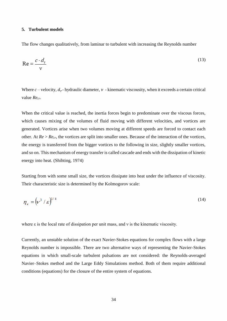
The flow changes qualitatively, from laminar to turbulent with increasing the Reynolds number
(13)
Where c – velocity, 𝑑𝑟- hydraulic diameter, 𝜈 - kinematic viscousity, when it exceeds a certain critical
value Recr.
When the critical value is reached, the inertia forces begin to predominate over the viscous forces,
which causes mixing of the volumes of fluid moving with different velocities, and vortices are
generated. Vortices arise when two volumes moving at different speeds are forced to contact each
other. At Re > Recr, the vortices are split into smaller ones. Because of the interaction of the vortices,
the energy is transferred from the bigger vortices to the following in size, slightly smaller vortices,
and so on. This mechanism of energy transfer is called cascade and ends with the dissipation of kinetic
energy into heat. (Shihting, 1974)
Starting from with some small size, the vortices dissipate into heat under the influence of viscosity.
Their characteristic size is determined by the Kolmogorov scale:
(14)
where ε is the local rate of dissipation per unit mass, and ν is the kinematic viscosity.
Currently, an unstable solution of the exact Navier-Stokes equations for complex flows with a large
Reynolds number is impossible. There are two alternative ways of representing the Navier-Stokes
equations in which small-scale turbulent pulsations are not considered: the Reynolds-averaged
Navier–Stokes method and the Large Eddy Simulations method. Both of them require additional
conditions (equations) for the closure of the entire system of equations.

35
The Reynolds-averaged Navier-Stokes method assumes the listing of the equations of transport of the
averaged flow (in time), with all the expected scales of turbulence. This approach significantly
reduces the computational resources which are needed for solving a numerical problem. If the
averaged flux is stationary, then the basic equations do not contain time derivatives, and the steady-
state solution is obtained more economically. A computational advantage is observed even for the
case of transient flow regime since the time step is determined by the global instability of the averaged
flow, rather than by turbulence.
The averaging method for the Navier-Stokes equations is highly used in the industry to solve
engineering problems and is uses several models of turbulence: Spalart-Allmaras, Reynolds Stress
Model (RSM), varieties of k-ε and original k-ε model and original k-ω model with varieties.
Large Eggy Simulation uses an alternative approach in which large vortices are solved in a non-
stationary formulation using the system of referred as "filtering" equations. The set of "filtering"
equations essentially serves to exclude sub-grid vortices from the calculation, i.e. vortices whose size
is smaller than the cells of the grid. As in the case of Reynolds-averaged Navier-Stokes method, the
filtration process requires the addition of special equations for the closure of the system of equations
of motion. The statistical values of the averaged flux, which are mostly of practical interest, are
presented as a function of time. The main advantage of the Large Eggy Simulation model is that it is
more accurate than other models for solving turbulent flows with a comparatively small Reynolds
number. However, it should be noted that the use of this model of turbulence requires sufficiently
high computational resources (Tucker, 2014).
Also, should be mentioned the fact that the application of the Large Eddy Simulation model in
industrial tasks is extremely limited. A typical application of this model was found only in simple
geometric areas, which is mainly due to the high requirements of this model for computational
resources. The LES model uses high-order spatial discretization, which allows a larger range of
turbulence scales to be resolved.
The Boussinesq hypothesis suggests a correspondence connecting Reynolds stresses with averaged
velocity gradients:

36
(15)
Which describes the linear connection between the Reynolds stress tensor and the strain rate tensor.
The drawback of the Boussinesq hypothesis is that the assumption of the isotropy of turbulent
viscosity is introduced, which is not always right-dimensional.
Models using the Boussinesq hypothesis are usually classified by the number of differential transfer
equations:
- models with one equation - Spalart-Allmaras model
- models with two equation - k-ε and k-ω models and models' variations
An alternative approach embodied in the Reynolds stress model is that the transfer equations of the
corresponding quantities are solved using the Reynolds stress tensor. As an additional equation, the
transport equation for the turbulent dissipation rate ε is used, which is necessary for determining the
turbulence mass scale. This means that for two-dimensional problems, 5 additional transport
equations are required, and 7 for three-dimensional ones (B. Anderson, 2011).
In many cases, models based on the Boussinesq hypothesis work well enough, and the use of the
RSM model is unjustified in terms of computational costs. However, the RSM model is indispensable
in situations where the anisotropy of the turbulent flow has a dominant effect on the averaged flux.
This occurs in high-speed rotating flows and flows with developed secondary currents, caused by the
inhomogeneity of the stress field.
Selecting the turbulent model depends on the turbulent flow required accuracy and computational
recourse and further the most relevant turbulent models will be explained deeply.
5.1. Spalart–Allmaras turbulence model
The model contains one differential equation with respect to the High Reynolds turbulent viscosity
associated with the turbulent viscosity by the algebraic ratio. Distance to the wall is used as a linear

37
turbulent scale. This model was developed for external aerodynamics problems, but it turned out that
its range of much wider applicability (Kuzmin, 2011).
It contains a few corrections which increase the applicability of the model:
- correction for curvature and rotation
- roughness correction
- non-linear version of the model
The basic Spalart-Allmaras model was considered as a model of turbulence for flows with a low
Reynolds number, which required good grid resolution in the boundary layer region.
In one of the 3D flow simulation software, the model was implemented in such a way that, in the case
of low resolution of the near-wall area, wall functions are used. In this case, this model is a good
choice for problems with a rough mesh. In addition, the gradients of the turbulent viscosity in the
near-wall regions, in this case, are much less than the gradients of the turbulence transfer
characteristics in the k-ε and k-ω models. This makes the model less sensitive to numerical errors
when the magnitude of the cell size gradient changes not smoothly in the near-wall region (Pope,
2000).
5.2. Standard k-ε model
The basic two-parameter model of turbulence with transport equations for turbulent kinetic energy k
and turbulent dissipation rate is mainly used for high intensive turbulent flows. The constant
coefficients for this model of turbulence are obtained experimentally, hence it is semi-empirical.
Despite the known limitations, the model has become widespread in industrial tasks, which is
explained by a stable iterative process, stability for errors, and reasonable accuracy for a huge amount
of turbulent flows. The Standard k-ε model was in the base of the improved versions of it, for instance,
RNG k-ε model and Relizable k-ε model (B. Anderson, 2011).
5.3. RNG k-ε model
There is a list of improvements which was done in this model in comparison with standard k-ε model:

38
- the effect of turbulence circulation is taken into account, which improves the accuracy of the
solution of high-speed rotating and circulating flows
- an analytical formula has been introduced to determine the dynamic viscosity, which makes
it possible to calculate turbulent flows with a lower Reynolds number more qualitatively, but
the set works with qualitative grid resolution in the boundary layer region
- an analytic dependence is introduced to calculate the Prandtl number for the flow, during the
solution, when in the standard k-ε model of turbulence this parameter is a constant
- an additional condition in the equation for the velocity of turbulent dissipation ε, which
improves the accuracy of solving highly stressed flows
- this feature makes the upgraded turbulent model more applicable and convenient for more
variants of calculations (Yeoh, 2010).
5.4. Realizable k-ε model
This model has several diversities in comparison with standard k-ε model:
- the equation of the velocity of turbulent dissipation is obtained from the exact equation of the
transfer of the root mean square pulsating vortex.
- an improved method for calculating turbulent viscosity was introduced
The term "Realizable" means that the model satisfies certain mathematical constraints of Reynolds
stresses that are assumed in turbulent flows.
The considerable advantage of the Realizable k-ε model is that it more accurately predicts the
distribution of the dissipation of flat and round jets. It is also likely to provide a better prediction of
rotating flows, boundary layers of pressure-sensitive gradients, separation currents and recirculation
flows. The realized k-ε model of turbulence has a drawback, which consists in that it overstates or
underestimates the turbulent viscosity of the flow, when the computational domain contains
simultaneously rotating and stationary regions (i.e., using multiple coordinate systems or sliding
grids). This is because the model uses the averaged rotation effect in determining the turbulent
viscosity. This additional rotational effect was tested for the case of a single rotating coordinate
system and the results showed a more accurate solution than in the case of the standard k-ε model of
turbulence (G. H. Yeoh, 2009).
39
5.5. Standard k-ω model
A two-parameter model of turbulence with equations for the turbulent kinetic energy k and the
turbulent dissipation rate. This model was developed by David C. Wilcox in 1998. Shows excellent
results for calculating wall layers and flows with a low Reynolds number (Pope, 2000).
5.6. Shear-Stress Transport (SST) model
This model is a variation of standard k-ω model and was developed by F.R. Menter. This model
effectively combines the stability and accuracy of the standard k-ω model in the near-wall regions
and the k-ε model at a distance from the wall, for this the k-ε model was converted into a version of
the k-ω model. The k-ω SST model has the following features in comparison with the standard k-ω
model:
- the definition of turbulent viscosity is modified, which is necessary for the representation of
the shear stress equation;
- the standard k-ω model and the transformed k-ε model are combined by a special function
and both are added to this model; a special function in the near-wall region takes the value of
unit that activates the standard k-ω model, and at a distance from the wall takes the value of
zero, which activates the transformed k-ε model;
- сonstants of turbulent models are different
These features make the k-ω SST model more reliable and accurate for a wide range of turbulent
flows (flows with hard analyzed pressure gradients, aerofoils and blade contours, transonic shock
waves) (Blazek, 2005).
5.7. Reynolds Stress Model (RSM) model
This model does not use the assumption of the isotropy of the turbulent viscosity, but for the closure
of the Navier-Stokes equations averaged over the Reynolds limit, solves the transport equations for
the Reynolds stresses in conjunction with the equation for the velocity of turbulent dissipation.
The RSM model describes the effects of curvature, twist, rotation, sharp changes in stresses between
layers, more rigorously than one- and two-parameter models of turbulence, it has a greater potential
for more accurate calculation of complex flows. However, the RSM model still has some

40
simplifications that were adopted to compose the Reynolds stress transfer equations, which was
necessary for closing the Navier-Stokes system of equations.
The use of this turbulence model is recommended in cases where the anisotropy of the turbulent flow
has a dominant effect on the nature of the turbulent flow (cyclones, highly swirling flows in
combustion chambers, rotating regions, secondary currents in channels which are the result of large
direct stresses). (Galaev, 2006)
41
6. Turbulent boundary layer modeling
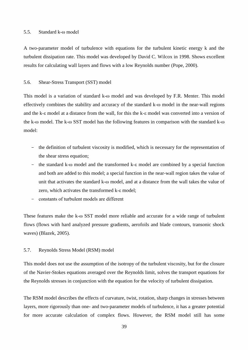
Figure 13 shows the structure of the boundary layer which contain 5 regions.
Figure 13 Boundary layer structure (Kirillov, 1974)
In the region of the viscous flow or internal flow (close to the wall domain), viscous forces dominate,
and the velocity profile does not depend on the Reynolds number and the pressure gradient. The
thickness of the region takes about 20% of the total thickness of the boundary layer and about 80%
of the total turbulence energy is generated in that region. The area consists of three layers: a viscous
sublayer (1), where the current can be considered laminar and viscosity plays a dominant role in heat
and mass transfer; buffer layer (2) and logarithmic layer (3), where turbulence intensifies the mixing
process.
In the region of the external flow, the velocity profile is determined from the averaged flow
parameters. The region consists of two layers: the wedge area (4) and the intermittency region (5). If
we assume that the logarithmic profile correctly approximates the change in velocity around the wall,
this makes it possible to quantify the shear stresses as a function of the velocity at given distances
from the wall (Kirillov, 1974).
42
The dimensionless distance from the wall to the first point of the computational grid 𝑌+ is plotted
along the x-axis:
(16)
Where y is the normal distance from the wall to the first grid node located in the stream
v – fluid kinematic viscosity
– is dynamic velocity
– is frictional stress on the wall
– fluid density
The selection how to model the grid depends on the choice of the turbulence model.
There are two types of grid designs, determined by the level of thickening of the grid cells to a solid
wall:
- Low-Reynolds number turbulent models
- High-Reynolds number turbulent
The level of cell thickening to solid walls is determined by the dimensionless distance y +models that
is shown in Figure 14.

43
Figure 14 Dimensionless distance y+ models
Thus, the calculated grids can be divided into 3 types:
1. fine mesh
2. mild mesh
3. mesh with wall functions
First two are low-Reynolds models, and mesh with wall functions is for high-Reynolds models.
High-grade models do not model the entire structure of the boundary layer, but use empirical
correspondence describing the flow near the wall. The main advantage of the method is that flow with
a high gradient of shear stresses in the boundary layer can be modelled with a relatively coarse
computational grid, which makes it possible to reduce the calculation time. Thus, the first design node
of the working grid must fall into the logarithmic layer (y+=30...300) (Matsson, 2014).
Low-Reynolds models calculate in detail the flow profile in the boundary layer with the help of very
small grid element sizes along the normal to the wall. Turbulence models based on the ω-equation,
such as the k-ω, SST or SMC model, allow this method to be used. This method can be used even in
simulating currents with very high Re numbers, as long as a viscous sublayer needs to be calculated.
The low-grade method requires a very fine grid near the wall (y + <2). The calculation time for this
method is correspondingly larger than for the wall function method (ANSYS 14.0, 2014).

44
7. Mesh generation
The development of numerical methods for gas dynamics calculations in such areas as a volute with
an outlet nozzle is of great importance. In these calculations, the calculation grid is very important.
While in areas of simple form, one can manage a single-block structured grid, in complex areas, it is
necessary to build multi-block grids, and to divide the region into simple subdomains, to construct
single-block grids in them and to interconnect them with each other. Automatically perform this
process for any geometry on this day is almost impossible. One of the methods for solving this
problem is the use of unstructured grids.
A characteristic feature of unstructured grids is the arbitrary arrangement of grid nodes in the physical
region. The arbitrariness of the arrangement of nodes is understood in the sense that there are no well-
defined grid directions, and not a grid structure similar to regular grids. The number of cells
containing each particular node can vary from node to node. In the two-dimensional case, the grid
nodes are combined into polygons, and in three-dimensional - into polyhedra. The plane uses
triangular and quadrangular cells, and in space - tetrahedra and prisms. The main advantage of
unstructured grids consists of greater flexibility in discretizing the physical area of a complex shape,
as well as in the possibility of fully automating their construction. For unstructured grids, local
condensations and adaptation of the grid to the solution are relatively easy to realize (Satofuka, 2000).
In the construction of design grids, the general recommendations used in the solution of gas-dynamic
problems are taken into account:
The grid should consist of elements with smooth changes in the size of the elements;
- the design grid should have a reduction in the dimensions of the elements in the wall region;
- it is recommended to use for calculations grid with cells, in which the angles formed by the
grid lines differ from the lines by no more than ± 45 °.

45
8. Boundary Conditions
A numerical experiment considers a stationary steady-state flow of a viscous compressible gas in the
stationary flow part of the second stage of the compressor. The calculation medium is air with the
law of density on an ideal gas. Under the conditions of the set task: Temperature of inlet gas is 30°C
and inlet pressure p is 1 bar, air can be regarded as an ideal gas.
Boundary conditions are settled in the inlet LID surface and shown in Figure 15, Figure 16, Figure
17.
Figure 15 Setting a boundary conditions for outlet pressure

46
At the output boundary of the calculated region, a constant total pressure condition is imposed for
each mode as 2,7 bar.
Figure 16 Setting a boundary condition for inlet mass flow
On solid surfaces, the condition of a solid wall is set, the properties of which are the impermeability
and adhesion of air molecules to it.

47
Figure 17 Setting a boundary condition for the walls

48
9. Solver Settings
The calculations were performed using the RANS turbulence model k- (the Navier-Stokes equations
averaged over the Reynolds are transformed to the form in which the effect of average velocity
fluctuations (in the form of turbulent kinetic energy) is added and the process of reducing this
fluctuation due to viscosity (dissipation).
The chosen model is one of the most stable and simple models of turbulence when flow calculations
are not expected in flow calculations.
The discretization of the spatial operators of the differential conservation equations is performed with
the second order of accuracy.

49
10. Quality of the solution
Solution quality depends on several factors which have been settled during the model creation. The
main factor is:
- solution convergence criteria
- assumptions
- mesh independence analysis
- analysis the influence of the turbulent model
10.1. Solution convergence criteria
The solution is converged when the difference between the new values from the previous iteration
does not exceed a certain value (in relative terms: 0.1% or 0.001%, etc.). For our stationary problems,
a satisfactory solution is a drop in the residual level to below 1.0e-03, good to below 1.0е-04 and
excellent to below 1.0e-05 (Tu, 2018). In the current calculations, good level of convergence was
reached.
10.2. Assumptions
To simplify the calculation, the following assumptions are made:
- there is no account for external heat transfer
- the influence of the previous stage of the compressor is not taken into account
- the roughness of the walls is not taken into account
The most significant is the first point since you can expect an overestimation of the value of the total
temperature in the simulation due to the neglect of external heat transfer.
Calculations which includes the external heat transfer is usually done on the final verification stage
of calculation. That is due to the fact that this kind of calculations require large computer capacities
and takes a long time.
Results and comparison of two variations with and without external heat transfer are presented in the
chapter “Result”

50
10.3. Mesh independence analysis
An important step in the calculations is the determination of the grid independence of the solution.
On the grid independence, the entire model was studied. Comparison results are shown in Table 1.
The analysis could be made according to pressure ratio data or compressor efficiency for a solution
with a different amount of cells in the mesh. In our case, the change in efficiency is not as significant
as pressure ratio.
Table 1 Mesh independence analysis
Simulation data
mesh inlet
pressure outlet
pressure pressure ratio
cells bar bar -
79831 1,022 2,7 2,641
323791 0,948 2,7 2,846
541798 0,938 2,7 2,876
1664285 0,936 2,7 2,883
Figure 18 Comparison of accuracy
As a result of mesh independence analysis for the current research was taken mesh with 323791 cells
with average imprecision 2%. Because of the optimal balance between accuracy versus calculation
time. Comparing the accuracy of results are shown in Figure 18.
2.6
2.65
2.7
2.75
2.8
2.85
2.9
0 500000 1000000 1500000 2000000
Pre
ssu
re r
atio
Number of mesh cells

51
Analysis of the current lines of the volute for calculation in air showed that a decrease in the size of
the cells makes it possible to more accurately map the regions of the computational region on which
the formation of vortices occurs. Since in the volute in most of the experiments and simulations there
is a formation of single or pair vortices, which lead to an increase in the loss factor, in calculating the
volute, the accuracy of the mapping of the vortex formation regions plays an important role. One of
the most challenging parts of mesh creation with comparative small cell size is cutwater part, which
is shown in Figure 19.
Figure 19 Cutwater part of volute with mesh

52
10.4. The influence of the turbulence model
Analysing the above graphs and flow patterns, a conclusion is drawn on the effect of the turbulence
model on the result of a numerical calculation of the volute part of the centrifugal compressor.
In the k-ε turbulence model, wall functions are used to calculate the wall velocity. This model has
fast convergence and relatively low memory requirements. A comparison with the characteristic of
the loss coefficient obtained from experimental data shows that the model of turbulence k-ε is not
very accurate in the simulation of flows in a region with a strongly curved geometry (F. Browand,
2009).
The k-ω model the flow dynamics has quite similar dynamic characteristics and behaviour as in the
k-ε model. In this model, wall functions are also used, so the requirements for memory resources are
the same as for the k-ε model. Convergence when using this model is slightly slower and essentially
depends on the initial approximation. The use of the k-ω model gives good results in those problems
where the k-ε model is not accurate enough. (Gulich, 2014).

53
11. Results
11.1. First numerical simulation
Calculations were done for seven types of volutes with different geometry of cross section flow path.
At the same time, in most of the models tree different theories were used for setting the area
distribution (Pfleiderer, Stepanoff and manual setting).
For faster convergence and receiving data firstly calculations were done on the rough mesh and then
results of this calculations were used as initial conditions in the high-quality mesh calculation.
In the following pictures represented velocity maps, total pressure distribution in the front and top
plane.
Model with thickness distribution according to Stepanoff theory (Figure 20)
Figure 20 Pressure and velocity distribution in the round cross section area volute according to
Stepanoff theory

54
Model of asymmetric round internal volute with a thickness distribution according to Pfleiderer
theory (Figure 21)
Figure 21 Pressure and velocity distribution in the asymmetric round internal cross section area
volute according to Pfleiderer theory

55
A drop shape model of the volute with a thickness distribution according to Pfleiderer theory (Figure
22).
Figure 22 Pressure and velocity distribution in the drop shape cross-section volute

56
Model of the round asymmetrical volute with a thickness distribution according to Stepanoff theory
(Figure 23).
Figure 23 Pressure and velocity distribution in the round asymmetrical cross section area volute
according to Stepanoff theory

57
Model of a trapezoid symmetrical volute with thickness distribution according to the Stepanoff theory
(Figure 24).
Figure 24 Pressure and velocity distribution in the trapezoid cross section area volute

58
A model with rectangular shaped volute with thickness distribution according to Stepanoff theory
(Figure 25).
Figure 25 Pressure and velocity distribution in the rectangular cross section area volute

59
A model with manually created shape of the cross section area (Figure 26).
Figure 26 Pressure and velocity distribution in the volute with manual settings cross section area
Comparison between the calculated variants was done according to the total pressure losses with
included percentage and pressure recovery ratio and represented in Table 2.

60
Table 2 Data received from the numerical simulation 1
var shape
total pressure losses delta static recovery ratio velocity relative mass flow inlet diff inl vol inl outlet volute volute inlet diff inl vol inl out volute outlet/inlet outlet
# - bar bar bar bar % bar bar bar bar bar % - m/s -
1 round 0,948 3,233 2,861 2,725 4,76% 0,136 0,938 1,969 2,543 2,7 5,82% 2,874 48,061 1
2 assym inter 0,956 3,259 2,859 2,735 4,33% 0,124 0,942 1,977 2,530 2,7 6,29% 2,861 51,509 1
3 drop 0,962 3,275 2,863 2,735 4,47% 0,128 0,947 1,987 2,527 2,7 6,39% 2,844 54,835 1
4 assym extern 0,954 3,247 2,852 2,733 4,18% 0,119 0,938 1,972 2,516 2,7 6,83% 2,865 53,580 1
5 trapezoid 0,958 3,257 2,861 2,722 4,88% 0,139 0,944 1,975 2,534 2,7 6,14% 2,841 51,392 1
6 square 0,956 3,257 2,869 2,733 4,73% 0,136 0,938 1,977 2,540 2,7 5,92% 2,858 51,354 1
7 manual 0,963 3,293 2,869 2,727 4,94% 0,142 0,948 1,990 2,543 2,7 5,81% 2,832 49,963 1
where, var is a number of volute variants, the shape is cross-section shape of the volute. Total pressure is represented in several control points:
inlet, diffuser inlet, volute inlet, outlet. Volute losses graph presents percentage losses, which have been reached in the volute. Volute delta shows
the real value of losses in the volute. Static pressure values are presented for the same control points as total pressure. Recovery is an increase of
static pressure percentagewise. Graph “ratio” shows pressure ratio between outlet total pressure and inlet total pressure. Velocity is representing
outlet velocity of the flow.
As it was mentioned in the eighth paragraph, the boundary conditions were settled for mass flow and static pressure, hence this parameters was the
same for all calculations for more relevant comparison of received data.

61
11.2. Second numerical simulation
The final design geometry of the compressor was calculated in the complex problem with included
water-cooling system, leakages and axial forces, which is represented in Figure 28 and Figure 27.
The calculation time of the problem was much longer than in the first numerical simulation since, the
model includes heat-transfer and fluid subdomain (water), and axial forces. So, that calculation is
done only for the final model of the stage.
Figure 27 Temperature distribution with OFF water-cooling system

62
Figure 28 Temperature distribution with ON water-cooling system
Using the water-cooling system allows increasing compressor efficiency by reducing the metal
temperature, hence decreasing temperature of the flow. Maximum air outlet temperature without a
water-cooling is 172°C; in case of using a water-cooling system, the outlet temperature is 145°C.

63
Figure 29 Temperature distribution in the outlet region of centrifugal compressor with OFF water-
cooling system
Figure 30 Temperature distribution in the outlet region of centrifugal compressor with ON water-
cooling system
In addition, the water-cooling system has a great impact on the seal temperature and diameter due to
the thermal expansion effect and shown in Figure 32 and Figure 31.

64
Figure 31 Temperature distribution in the seal area with OFF water-cooling system
Figure 32 Temperature distribution in the seal area with ON water-cooling system
In the course of numerical simulation of this problem was used the same boundary conditions and,
the following data were obtained and shown in Table 3.

65
Table 3 Data received from the numerical simulation 2
total pressure static pressure inlet outlet inlet outlet ratio
bar bar bar bar -
0.96 2.72 0.95 2.7 2.842
11.3. Verification with experimental data
The geometry of the final model was made, assembled and tested in an experimental laboratory.
Measurements were done every ten seconds after stabilizing temperatures and rotational speed. On
the presented Table 4 results shown of the specific regime which is correlated to boundary conditions
of calculation. Working characteristics of the compressor were closest in terms of rotation speed and
output pressure during that five experimental points. The compressor was tested for several regimes
from the surge to chock line. For more convenient analysis of experimental data, the table included
only graphs, which is corresponded to the matched mass flow rate and rotational speed. Results are
presented in Table 4.
Table 4 Experimental data
speed Inlet imp out outlet ratio
relative
mass flow
rpm bar bar bar
34000 0,994 1,990 2,780 2,797 1,009
34000 0,994 1,996 2,796 2,812 0,994
34000 0,994 1,995 2,803 2,820 0,996
34000 0,994 1,998 2,815 2,833 0,997
34000 0,994 2,001 2,827 2,844 0,999
Comparison the experimental data with numerical simulation shows good correlation of numerical
simulation.

66
12. Conclusion
The work is devoted to the improvement of the design procedure for the volute of centrifugal
compressors based on verification of the volute calculation data obtained with the Solidworks
software package with experimental data. Dependences of the loss coefficient on the geometry of the
volute of the centrifugal compressor are obtained. The objects of the investigation were the
compressor stage with different volutes.
Flow calculations in the volute are carried out in one mode according to the mass flow rate.
A study was conducted on "grid independence" - the results for calculated grids with a different
number of elements were compared. Optimal (from the point of view of "accuracy - calculation time")
the number of elements of the grid 315 000 – 375 000 elements for the impeller, the spiral chamber
and the diffuser sector.
Verification of the calculation results was done using data obtained on the basis of the experiment.
Verification was carried out on the basis of analysis of the characteristics of the losses factor of the
volute from the mass flow coefficient. Comparison of the characteristics of the volute obtained as a
result of modelling with experimental data showed a qualitative coherence.
The quantitative discrepancy between the calculation results is explained by the "idealization" of the
boundary conditions specified in the simulation. Within the framework of the work, a change in the
geometry of the compressor’s volute was performed. The change in the geometry of the spiral
chamber consisted of a change in the shape of its entrance section. Based on the results of calculations
of the changed geometry of the volute, flow patterns and characteristics of the loss coefficients.
It is concluded that in the volute designing process it is important to pay attention to the flow
characteristics as well as to take into account the loss factor, in order to avoid additional losses in the
flow braking in advance due to the inaccessibility of the cross section, and also to avoid the
appearance of stagnant zones and vortices.
Also, correct numerical simulation provides a reliable picture of the flow, and gas-dynamic
characteristics, received from the results of modelling, are well correlated with experimental data.

67
References
ANSYS 14.0. (2014). User manual.
B. Anderson, R. A. (2011). Computentional fluid dynamics for engineeres. Cambridge university
press.
Blazek. (2005). Computantional fluid dynamics: principles and applications. Elsevier.
Bloch, H. P. (1995). A prictical guide to compressor technology.
Cheng Xu, M. M. (2005). Development and Design of a Centrifugal Compressor Volute.
International Journal of Rotating Machinery, 190-196.
Cipollone, R. (2015). Carbon and energy saving markets in compressed air. IOP Conference Series:
Materials Science and Engineering, Volume 90, conference 1. .
Deiter K. Huzel, D. H. (1992). Modern Engineering for Design of Liquid-propellant Rocket Engines.
AIAA.
Den, G. (1973). Flow mechanics in centrifugal compressors. (In russian) Mekhanika potoka v
tsentrobezhnykh kompressorakh. Leningrad: Mashinostroenie.
F. Browand, R. M. (2009). The Aerodynamics of Heavy Vehiles. Springer.
G. H. Yeoh, K. Y. (2009). Computentional fluid dynamics for fire engineering. Elsevier.
Galaev, S. (2006). Chislennoye modelirovaniye techeniya vyazkogo gaza v reshetkakh osevykh
turbomashin: metodika i rezul'taty primeneniya sovremennykh programmnykh sredstv. (In
russian). Saint Petersburg: SPBGPU.
Gulich, J. F. (2014). Centrifugal Pumps. Springer.
H.K. Versteeg, W. M. (2007). An Introduction to computantional fluid dynamics. The Finite Volume
Method. Glasgow.
Hanlon, P. C. (2001). Compressor handbook.
J. H. Ferziger, M. P. (2002). Computantional Methods for Fluid Dynamics. Berlin: Springer.
Japiske D., B. N. (1994). Introduction to Turbomachinery.

68
Kirillov. (1974). Theory of turbomachines (In russian) Teoriya turbomashin. Leningrad:
Mashinostroenie.
Kreuzfeld G, M. R.-P. (2011). Designing new compressors from scratch and compressor redesign.
CompressorTech Two Magazin.
Kuzmin, A. (2011). Computantional Fluid Dynamics 2010. Springer.
Ludtke, K. H. (2004). Process Centrifugal Compressors. Springer.
M. Hamada, S. T. (1994). Flow measurement a fan volute tonque using particle tracking velocimetry.
Power and Energy pt. A, 235-246.
Matsson, J. E. (2014). An introduction to SolidWorks Flow Simulation 2014. SDC Publications.
Miftahov. (1980). Research, calculation and design of output devices of centrifugal compressors. (In
russian) Issledovaniye, raschet i proyektirovaniye vykhodnykh ustroystv tsentrobezhnykh
kompressorov. Kazan.
Miftahov, A. (1996). Inlet and outlet devices of centrifugal compressors (on Russian Language).
Kazan.
Nikitin, C. (1979). Calculation of losses in the output device of a centrifugal compressor. (In russian)
Raschet poter 'v vykhodnom ustroystve tsentrobezhnogo kompressora. Moscow:
Energomashinostroenie.
Pfleiderer, C. (1955). Die Kreiselpumpen für Flüssigkeiten und Gase. Berlin: Springer–Verlag.
Pope, S. B. (2000). Turbulent flows. Cambridge: Cambridge university press.
R. Dong, S. C. (1997). Effect of Modification to Tongue and Impeller Geometry on Unsteady Flow
Pressure Fluctuations and Noise in a Centrifugal Pump. ASME J. Turbomach. .
Rama S. Gorla, A. A. (2003). Turbomachinery design and theory.
Satofuka, N. (2000). Computantional Fluid dynamics 2000 vol.2 . Springer.
Shihting. (1974). Theory of the boundary layer. (In russian) Teoriya pogranichnogo sloya. Moscow:
Nauka.

69
Stepanoff, A. J. (1957). Centrifugal and Axial Flow Pumps: Theory, Design and Application. New
York: Wiley.
Tu, J. (2018). Computantional Fluid Dynamics, A Practical Approach. Elsevier.
Tucker, P. (2014). Unsteady Computentional Fluid Dynamics in Aeronautics. Springer.
Tuzson, J. (2000). Centrifugal Pump Design. John Wiley & Sons .
Un, C. (2012). Numerical simulation of three-dimensional flow in a spiral chamber based on the k-
epsilon turbulence model. (In russian) Chislennoye modelirovaniye trekhmernogo techeniya
v spiral'noy kamere na osnove modeli turbulentnosti k-epsilon. Omsk: OmGTU.
Van Elburg, M. V. (2017). Preparatory study on Low pressure & Oil-free Compressor Packages.
European Commission, Directorate-General for Energy, 289 p.
Wild, T. W. (2018). Aircraft powerplants.
Yeoh, G. H. (2010). Computentional techniques for multi-phase flows. Elsevier.