OPTIMIZATION USING TOPOLOGICAL DERIVATIVE AND BOUNDARY

ELEMENT METHOD WITH FAST MULTIPOLE

L. M. Braga1, C. T. M Anflor

2 , E. L. Albuquerque

1

1 Departamento de Engenharia Mecânica, Universidade de Brasília, Campus Universitário

Darcy Ribeiro, Brasilia, DF, Brasil, (eder@unb.br)

2 Engenharia Automotiva, Universidade de Brasília, Campus Gama, DF, Brasil,

(anflor@unb.br )

Abstract. The objective of this work is to compare topologies resulting from direct BEM

(Boundary Element Method) with a BEM accelerated by Fast Multipole Method (FMM). A

formulation of fast multipole boundary element (FMBEM) is introduced in order to turn the

optimization process more attractive in the point of view of the computational cost. The

formulation of the fast multipole is briefly summarized. A topological-shape sensitivity

approach is used to select the points showing the lowest sensitivities, where material is

removed by opening a cavity. As the iterative process evolves, the original domain has holes

progressively removed, until a given stop criteria is achieved. A benchmark is investigated by

imposing different FMBEM parameters. For effect of comparison the topology resulting from

an analytical BEM optimization process is used. The topologies resulting due to this set of

parameters imposed are presented. The CPU time x DOF’s are also investigated. The

accelerated BEM demonstrated good feasibility in an optimization routine.

Keywords: Topology optimization, topological derivative, fast multipole method, boundary

element methods.

1. INTRODUCTION

Although the Boundary Element Method (BEM) provides some facilities when

modeling many problems its efficiency is not suitable for large-scale models. The BEM in

general produces dense and non-symmetric matrices that, in spite of smaller in sizes, requires

O(N2) operations to compute the coefficients. In order to solve the resulting system using

direct solvers another O(N3) operations is also required. In order to overcome this

inefficiency a coupling between Fast Multipole Method (FMM) and BEM is purposed. This

will allow solving problems with several millions of degree of freedom (DOF’s). Generally

for large scales models the Finite Element Method (FEM) was indicated to solve models with

several millions of DOF’s, on the other side, the BEM has been limited to solving problems

with a few thousands DOF’s for many years. In the last years great efforts has been done by

Blucher Mechanical Engineering ProceedingsMay 2014, vol. 1 , num. 1www.proceedings.blucher.com.br/evento/10wccm

scientists to improve the BEM maintaining its all attractive, such as, easy mesh in modeling,

small matrices of coefficients, no mesh dependency. The next step relies on expand the

method to solve problems of large-scale. An example of large-scales is the topology

optimization problem. As it is an iterative problem, a number of elements are always

increasing because the material is being removed and a significantly number of DOF’s must

be solved. In the point of view of computational cost it should be a serious problem especially

when the case under investigated has its statement in 3D optimization. During the last years

many efforts have been done in order to accelerate the BEM for large-scales problems. As

pioneers [1,2] presented the FMM which promised the accelerating the solutions of BIE. The

main goal was to reduce the CPU time in FMM accelerated BEM to O(N). Thereafter this

new technique was applied for solving elasticity [3] and fluids [4] problems in large-scale.

Some years after, [5] announced the FMM as one of the top algorithms in scientific

computing that were developed in the 20th century. In this publication the authors had

developed a complete tutorial which presents the basic concept and the main procedures in the

FMM for solving boundary integral equations for 2D potential problems. The author [6]

extended the FMM formulation for large-scale analysis of two-dimensional (2D) Stokes flow

problems. For solving the dual Boundary Integral Equation (BIE) formulation, the author had

employed a linear combination for velocity and the hipersingular BIE for traction to attain a

better conditioning for the BEM system of equations. Some examples were presented and

showed a good accuracy and efficiency of the proposed approach. Also [7] published the

book entitle Fast Multipole Boundary Element Method where many instructions are given in

order to provide fundamentals for others researches can implement this method. The FMM

was implemented by [8] for solving the effective thermal conductivity (ETC) of random

micro-heterogeneous materials using representative elements and FMBEM. The main goal of

this paper is to implement the FMM in a topology optimization code. The idea relies on

compare the performance of both methodologies, i.e., optimization with Direct BEM against

FMBEM in the point of view of CPU time and resulting topologies. This paper is organized

as follow: In Section 2 the main idea of TD is discussed and the analytical expressions for

TD in Poisson problems are presented. In Section 3 and 4 the methods BEM and FMBEM for

2D potential problem is shown, respectively. In Section 5 some numerical examples and their

respectively results are presented. Finally, in Section 6 this work is concluded and some

discussions are carrying on.

2. TOPOLOGICAL DERIVATIVE

A topological derivative for Poisson Equation is applied in this work for determining

the domain sensitivity. A simple example of applicability consists in a case where a small

hole of radius (ε) is open inside the domain. The concept of topological derivative consists in

determining the sensitivity of a given function cost (ψ) when this small hole is increased or

decreased. The local value of TD at a point ( x ) inside the domain for this case is evaluated

by:

*

0

( ) ( )( ) lim ,

( )TD x

f

ε

ε

ψ ψ

ε→

Ω − Ω= (1)

where ψ(Ω) and ψ(ε) are the cost function evaluated for the original and the perturbed

domain, respectively, and f is a problem dependent regularizing function. By eq (1) it is not

possible to establish an isomorphism between domains with different topologies. This

equation was modified introducing a mathematical idea that the creation of a hole can be

accomplished by single perturbing an existing one whose radius tends to zero. This allows the

restatement of the problem in such a way that it is possible to establish a mapping between

each other [9].

*

0

( ) ( )( ) lim ,

( ) ( )T

D xf f

ε δε ε

εε δε ε

ψ ψ+

→+

Ω − Ω=

Ω − Ω (2)

where δε is a small perturbation on the holes’s radius. In the case of linear heat

transfer, the direct problem is stated as:

Solve |u k u bε ε− ∆ = on εΩ

(3)

subjected to:

( )

on

on

- on ,

D

N

c R

u u

uk q

n

uk h u u

n

ε

εε ∞

= Γ

∂= Γ

∂∂

= Γ∂

(4)

Where,

( ) ( ) ( ), , 0c

D irich le t N eum ann R ob in

u uh u u k q k h u u

n n

ε ε ε εε εε εα β γ α β γ ∞

∂ ∂ = − + + + + − = ∂ ∂

(5)

is a function which takes into account the type of boundary condition on the holes to

be created ( ,u

u qn

εε ε

∂=

∂are the temperature and flux on the hole boundary, while u

ε∞

and chε

are the hole’s internal convection parameters, respectively). After an intensive analytical

work, it was developed explicit expressions for TD for problems governed by eq (3). Table 1

summarizes the final expressions for topological derivative, considering the three classical

cases of boundary conditions on the holes.

Table 1. Topological derivative for the various boundary conditions prescribed on the holes.

BOUNDARY CONDITION ON THE HOLE TOPOLOGICAL DERIVATIVE EVALUATED AT

Neumann homogeneous boundary condition

(α = 0, β =1 , γ = 0) ( )

TD x k u u bu= ∇ ∇ − x ∈ Ω ∪ Γ

Neumann non-homogeneous boundary condition

(α = 0, β =1 , γ = 0) ( )

TD x q uε= − x ∈ Ω ∪ Γ

Robin boundary condition

(α = 0, β = 0, γ = 1) ( )( )T cD x h u u

εε ∞= − x ∈ Ω ∪ Γ

Dirichlet boundary condition

(α = 1, β = 0, γ = 0) ( )1( )

2T

D x k u uε= − − x ∈ Ω

Dirichlet boundary condition

(α = 1, β = 0, γ = 0) ( )

TD x k u u buε= ∇ ∇ − x ∈ Γ

3. BEM

A brief review on Boundary element method using constant elements is summarized in

this work. An initial domain is established with boundary conditions prescribed on its

boundary. Considering a Laplace equation governing a 2D potential problems:

;,0)(2 Ω∈∀=∇ xxu (6)

Fig.1 Domain Ω and its boundary Γ.

For a potential problem three kinds of boundary conditions may be imposed, Dirichlet,

Neumann and/or Robin. For this presentation the first and second boundary conditions are

imposed,

2

1

),()()(

;),()(

Γ∈∀=∂

∂=

Γ∈∀=

xxqxu

xq

xxuxu

η

(7)

Where u is the potential field in domain (Ω), Γ is the boundary of Ω, n is the outward

normal. Note that the barred quantities are the values imposed by the boundary conditions on

the boundary. The solution of eq.(6) under boundary conditions as eq.(7) is:

Ω∈∀−= ∫ xydSyuyxqyqyxuxuS

),()(),()(),([)( ** (8)

Where ),(*yxu and ),(*

yxq are the Green’s function for 2D problems

ηπη ∂

∂=

∂

∂=

r

ry

yxuyxq

2

1

)(

),(),(

**

(9)

and r represents the distance between the collocation point x and the field point y, as depicted

in fig.1. Taking x belongs to the Γ the classic BIE formulation of BEM [10] is obtained as:

;),()(),()(),([)()( ** Γ∈∀−= ∫ xydSyuyxqyqyxuxuxCS

(10)

If the boundary is smooth in the collocation point x, the coefficient C(x) = 1/2. The

next step consists in discretize the boundary Γ using N constant elements as illustrated by fig.

2.

x

Γ2

Γ1 Γ= Γ1 U Γ2

n y

Ω

r

Figure 2. Discretization of the boundary Γ using constant elements.

The discretized equation of BIE is now presented as,

;,...,3,2,1,ˆ2

1

1 1

NiuHqGuN

j j

jijjiji =

−=∑ ∑

= =

(11)

Where the uj and qj (j = 1,2,…,N) are the nodal values of the u and q in the element ∆Sj,

respectively. Applying the boundary conditions (2) at each node and switching the columns

for grouping the unknowns variables one finds,

BA =λ (12)

And where A is the coefficients matrix, λ the unknown vector and b the known right-

hand side vector.

4. FAST MULTIPOLE BOUNDARY ELEMENT

BEM uses the Green’s functions as the weighting function on its formulation which

increase the accuracy when compared with another numerical techniques [10]. As a result the

spatial dimension is reduced by one. Additionally, the computational cost of a traditional

BEM direct can be reduced by using the FMBEM. The goal of FMM relies on translating

node-to-node interactions to cell-to-cell interactions. These cells have a hierarchical structure

called as tree while the small ones are called as leaves. FMM employs iterative equations

solvers (GMRES) where matrix-vector multiplications are calculated using fast multipole

expansions. As iterative equations are used some parameters for the FMM, such as, maximum

number of elements allowed in a leaf (maxl) and in the tree structure (levmax), number of

terms in multipole expansion (nexp) and local expansion (ntylr), and also the GMRES

solution convergence (tol) must be set. The expansions used for 2D potential problem for

FMM are briefly summarized as table 2. Further details about the analytical derivations

should be attained in [5,7].

Γ2

Γ1

Γ= Γ1

U Γ2

n y

Ω

r

x

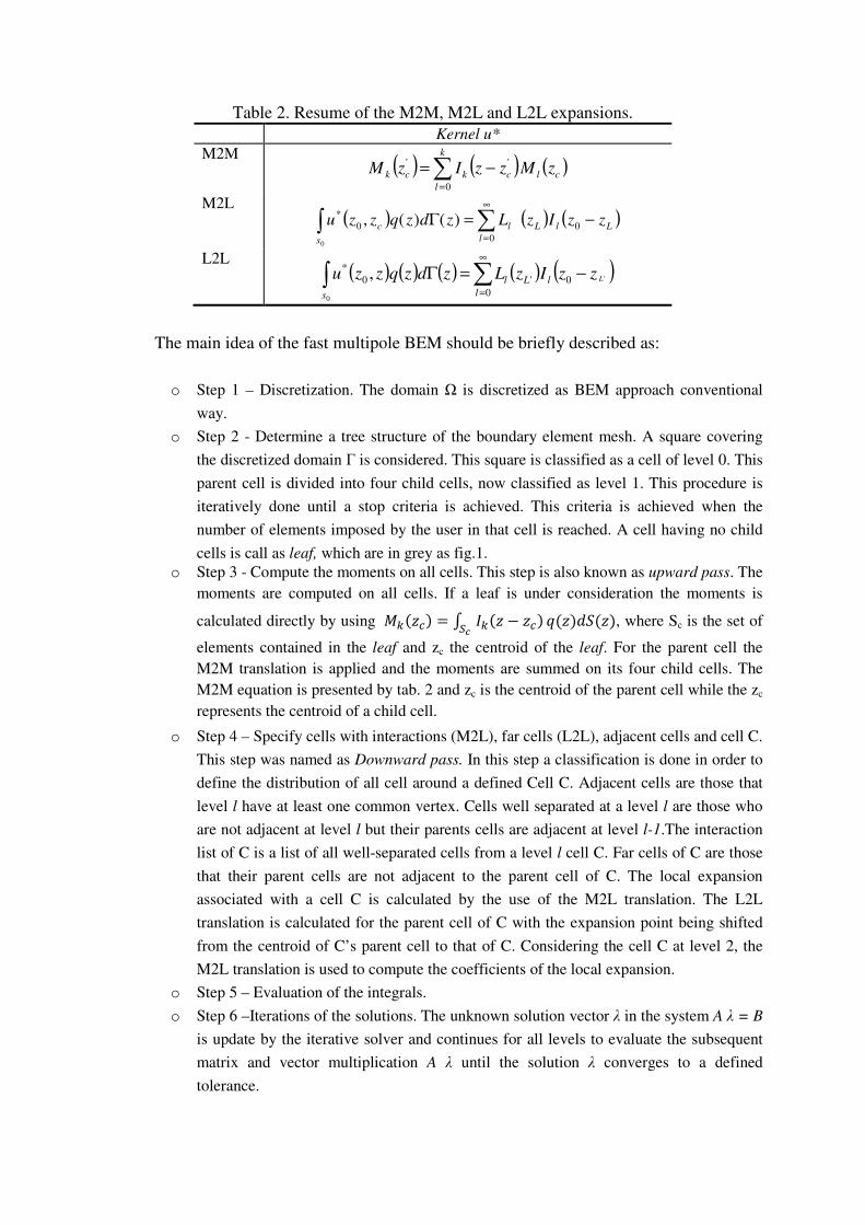
Table 2. Resume of the M2M, M2L and L2L expansions.

Kernel u*

M2M ( ) ( ) ( )cl

k

l

ckck zMzzIzM ∑=

−=0

''

M2L ( ) ( ) ( )

LlL

l

l

s

c zzIzLzdzqzzu −=Γ ∑∫∞

=0

0

0

*

0

)()(,

L2L ( ) ( ) ( ) ( ) ( )'

0

0'

0

0

* , LzzIzLzdzqzzu lL

l

l

s

−=Γ ∑∫∞

=

The main idea of the fast multipole BEM should be briefly described as:

o Step 1 – Discretization. The domain Ω is discretized as BEM approach conventional

way.

o Step 2 - Determine a tree structure of the boundary element mesh. A square covering

the discretized domain Γ is considered. This square is classified as a cell of level 0. This

parent cell is divided into four child cells, now classified as level 1. This procedure is

iteratively done until a stop criteria is achieved. This criteria is achieved when the

number of elements imposed by the user in that cell is reached. A cell having no child

cells is call as leaf, which are in grey as fig.1.

o Step 3 - Compute the moments on all cells. This step is also known as upward pass. The

moments are computed on all cells. If a leaf is under consideration the moments is

calculated directly by using = − , where Sc is the set of

elements contained in the leaf and zc the centroid of the leaf. For the parent cell the

M2M translation is applied and the moments are summed on its four child cells. The

M2M equation is presented by tab. 2 and zc is the centroid of the parent cell while the zc

represents the centroid of a child cell.

o Step 4 – Specify cells with interactions (M2L), far cells (L2L), adjacent cells and cell C.

This step was named as Downward pass. In this step a classification is done in order to

define the distribution of all cell around a defined Cell C. Adjacent cells are those that

level l have at least one common vertex. Cells well separated at a level l are those who

are not adjacent at level l but their parents cells are adjacent at level l-1.The interaction

list of C is a list of all well-separated cells from a level l cell C. Far cells of C are those

that their parent cells are not adjacent to the parent cell of C. The local expansion

associated with a cell C is calculated by the use of the M2L translation. The L2L

translation is calculated for the parent cell of C with the expansion point being shifted

from the centroid of C’s parent cell to that of C. Considering the cell C at level 2, the

M2L translation is used to compute the coefficients of the local expansion.

o Step 5 – Evaluation of the integrals.

o Step 6 –Iterations of the solutions. The unknown solution vector λ in the system A λ = B

is update by the iterative solver and continues for all levels to evaluate the subsequent

matrix and vector multiplication A λ until the solution λ converges to a defined

tolerance.

Figure 1 depicts the basic idea of the FMM in steps.

Figure 1. FMM Scheme.

4. NUMERICAL RESULTS

The high computational effort involved in an optimization process motivates the

implementation of FMM in order to maintain those attractive characteristics when coupling

BEM and DT [11]. The topology optimization process is carried out using an Intel Pentium

Step 4 – M2M

Step 1 – Initial Domain – level 0

Γ

Ω

2

3

1

4

12 16

14 15

10

5

11

9 8

6

13

7

Step 2 Discretization – Level 1 Step 2 Discretization – Level 2

Step 2 – Discretization – Level 3

28

2

31

27

29

11

21 23

24

30

29

20

28

2

25

3

Step 3 – Multipole expansion

Step 4 – M2L and L2L – level 2

M2L

L2L

Cell C

M2L

Cell C

M2L level

Step 4 – M2L level 3 Step 5 – Evaluation of all integrals

core 2 Duo with 4GB of RAM and 2,93GHz. This section presents one example that

demonstrates the application of the proposed method. The results obtained for each case are

compared with Direct BEM versus FMBEM. During the optimization process the

computational cost, number of DOFs and volume were taken into account. For a specific

iteration the respective intermediary topology is illustrated. The iterative process was halted

when a given amount of material was removed from the original domain. In all cases the total

potential energy was used as the cost function. A regularly-spaced grid of internal points was

generated automatically, taking into account the radius of the holes created during each

iteration. The radius was obtained as a fraction of a reference dimension of the domain (r = ω

lref). In all cases lref = min (height,width) was adopted. The objective in all cases was to

minimize the material volume. The current volume of the domain (Vf) was checked at the end

of each iteration until a reference value was achieved (Vf = φ V0, where V0 represents the

initial volume and φ a defined percentage of material to be removed).

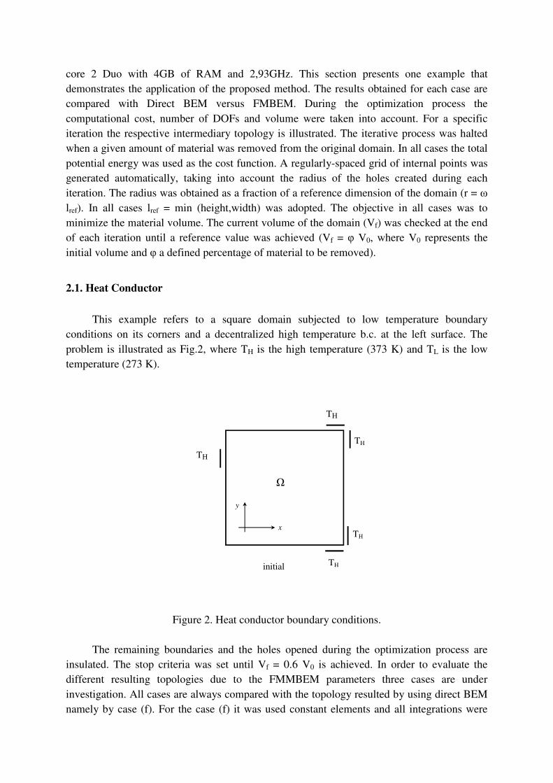
2.1. Heat Conductor

This example refers to a square domain subjected to low temperature boundary

conditions on its corners and a decentralized high temperature b.c. at the left surface. The

problem is illustrated as Fig.2, where TH is the high temperature (373 K) and TL is the low

temperature (273 K).

Figure 2. Heat conductor boundary conditions.

The remaining boundaries and the holes opened during the optimization process are

insulated. The stop criteria was set until Vf = 0.6 V0 is achieved. In order to evaluate the

different resulting topologies due to the FMMBEM parameters three cases are under

investigation. All cases are always compared with the topology resulted by using direct BEM

namely by case (f). For the case (f) it was used constant elements and all integrations were

initial

Ω

TH

x

y

TH

TH

TH

TH

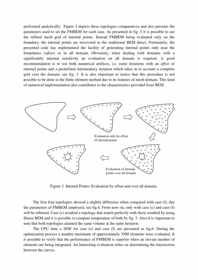
performed analytically. Figure 3 depicts these topologies comparatives and also presents the

parameters used to set the FMBEM for each case. As presented in fig. 3 it is possible to see

the refined mesh grid of internal points. Instead FMBEM being evaluated only on the

boundary, the internal points are recovered as the traditional BEM direct. Fortunately, the

presented code has implemented the facility of generating internal points only near the

boundaries (offset) or in all domain. Obviously, when dealing with domains with a

significantly internal sensitivity an evaluation on all domain is required. A good

recommendation is to use both numerical artifices, i.e. some iterations with an offset of

internal points and a predefined intermediary iteration which takes in to account a complete

grid over the domain, see fig. 3. It is also important to notice that this procedure is not

possible to be done in the finite element method due to its features of mesh domain. This kind

of numerical implementation also contributes to the characteristics provided from BEM.

Figure 3. Internal Points: Evaluation by offset and over all domain.

The first four topologies showed a slightly difference when compared with case (f), due

the parameters of FMBEM employed, see fig.4. From now on, only with case (c) and case (f)

will be refereed. Case (c) resulted a topology that match perfectly with those resulted by using

Direct BEM and it is possible to compare temperature of both by fig. 5. Also it is important to

note that both topologies attained the same volume at the same iteration.

The CPU time x DOF for case (e) and case (f) are presented as fig.6. During the

optimization process a number maximum of approximately 3500 elements were evaluated. It

is possible to verify that the performance of FMBEM is superior when an elevate number of

elements are being integrated. An interesting evaluation relies on determining the intersection

between the curves.

Evaluation only by offset

of internal points

Evaluation of internal

points over all domain

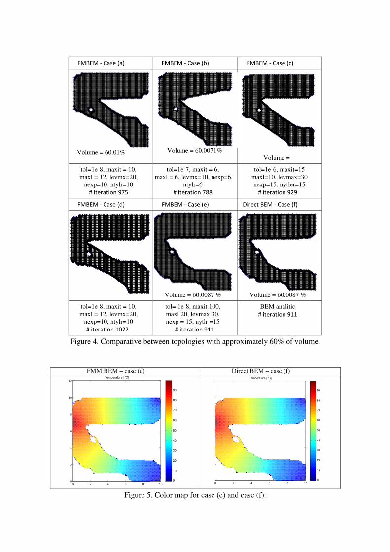
FMBEM - Case (a) FMBEM - Case (b) FMBEM - Case (c)

Volume = 60.01%

Volume = 60.0071%

Volume =

tol=1e-8, maxit = 10,

maxl = 12, levmx=20,

nexp=10, ntylr=10

# iteration 975

tol=1e-7, maxit = 6,

maxl = 6, levmx=10, nexp=6,

ntylr=6

# iteration 788

tol=1e-6, maxit=15

maxl=10, levmax=30

nexp=15, nytler=15

# iteration 929

FMBEM - Case (d) FMBEM - Case (e) Direct BEM - Case (f)

Volume = 60.0087 %

Volume = 60.0087 %

tol=1e-8, maxit = 10,

maxl = 12, levmx=20,

nexp=10, ntylr=10

# iteration 1022

tol= 1e-8, maxit 100,

maxl 20, levmax 30,

nexp = 15, nytlr =15

# iteration 911

BEM analitic

# iteration 911

Figure 4. Comparative between topologies with approximately 60% of volume.

FMM BEM – case (e) Direct BEM – case (f)

Figure 5. Color map for case (e) and case (f).

0 2 4 6 8 100

2

4

6

8

10

12Temperature [°C]

0

10

20

30

40

50

60

70

80

90

0 2 4 6 8 100

2

4

6

8

Temperature [°C]

0

10

20

30

40

50

60

70

80

90

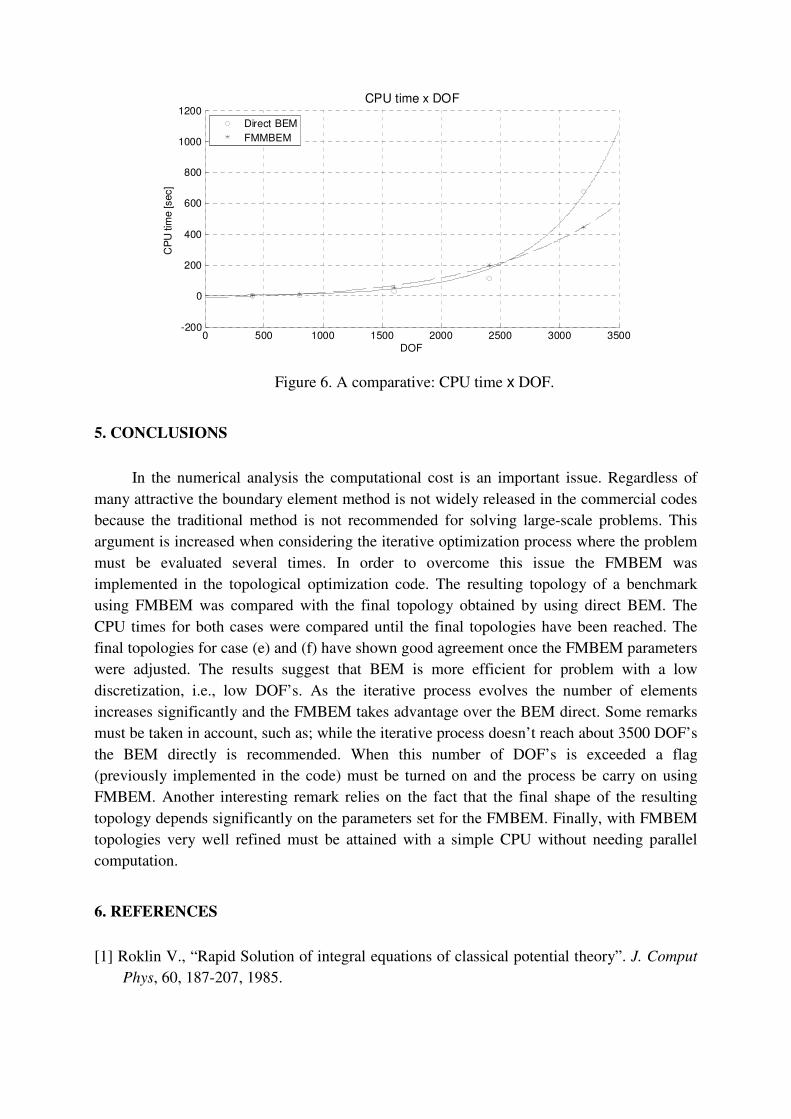
Figure 6. A comparative: CPU time x DOF.

5. CONCLUSIONS

In the numerical analysis the computational cost is an important issue. Regardless of

many attractive the boundary element method is not widely released in the commercial codes

because the traditional method is not recommended for solving large-scale problems. This

argument is increased when considering the iterative optimization process where the problem

must be evaluated several times. In order to overcome this issue the FMBEM was

implemented in the topological optimization code. The resulting topology of a benchmark

using FMBEM was compared with the final topology obtained by using direct BEM. The

CPU times for both cases were compared until the final topologies have been reached. The

final topologies for case (e) and (f) have shown good agreement once the FMBEM parameters

were adjusted. The results suggest that BEM is more efficient for problem with a low

discretization, i.e., low DOF’s. As the iterative process evolves the number of elements

increases significantly and the FMBEM takes advantage over the BEM direct. Some remarks

must be taken in account, such as; while the iterative process doesn’t reach about 3500 DOF’s

the BEM directly is recommended. When this number of DOF’s is exceeded a flag

(previously implemented in the code) must be turned on and the process be carry on using

FMBEM. Another interesting remark relies on the fact that the final shape of the resulting

topology depends significantly on the parameters set for the FMBEM. Finally, with FMBEM

topologies very well refined must be attained with a simple CPU without needing parallel

computation.

6. REFERENCES

[1] Roklin V., “Rapid Solution of integral equations of classical potential theory”. J. Comput

Phys, 60, 187-207, 1985.

0 500 1000 1500 2000 2500 3000 3500-200

0

200

400

600

800

1000

1200CPU time x DOF

DOF

CP

U ti

me [sec]

Direct BEM

FMMBEM

[2] Greengard L.F., “The rapid evaluation of potentials fields in particle systems”,

Cambridge: The MIT Press, 1988.

[3] Peirce A.P., Napier J.A.L. A spectral multipole method for efficient solutions of large

scale boundary element models in elastostatics. Int J Numer Meth Eng. 38, 4009-4034,

1995.

[4] Mammoli A. and Ingber M., “Stokes flow around cylinders in a bounded two-dimensional

domain using multipole accelerated boundary element methods”, International Journal

for Numerical Methods in Engineering, 44, 897-917 (1999).

[5] Liu Y.J., Nishimura N., “The fast multipole boundary element method for potential

problems: A tutorial”. Engineering Analysis with Boundary Elements, 30, 371-381, 2006.

[6] Liu Y.J., “A new fast multipole boundary element method for solving 2-D Stokes flow

problems based on a dual BIE formulation”. Engineering Analysis with Boundary

Elements, 32, 139-151, 2008.

[7] Liu Y.J., “Fast Multipole Boundary Element Method: Theory and applications in

Engineering”, Cambridge 2009.

[8] Dondero M., Cisilino A.P., Carella J.M., Tomba J. P., “Effective thermal conductivity of

functionally graded random micro-heteregeneous materials using representative volume

element and BEM”. International Journal of Heat and Mass transfer, 54, 3874-3881

2011.

[9] Feijóo R., Novotny A., Taroco E., Padra C., “The topological derivative for the Poisson’s

problem”. Mathematical Model and Methods in Applied Sciences, 13, 1825-1844, 2003.

[10] Wrobel L.C. and Aliabadi M.H, “The Boundary Element Method, Vol2: Applications in

Solids and Structures”, Wiley 2002.

[11] Anflor C.T.M., Marczak R.J., “Topological optimization of anisotropic heat conducting

devices using Bézier-smoothed Boundary Representation”. Computer Modeling in

Engineering & Sciences (Print), 1970, 151-168, 2011.