Optimization of the Sizing of a Solar Thermal Electricity Plant:Mathematical Programming Versus Genetic Algorithms

José M. Cabello, José M. Cejudo, Mariano Luque, Francisco RuizUniversity of Málaga

Campus El Ejido s/n, 29071 Málaga, Spainjmcabello@uma.es, jmcejudo@uma.es, mluque@uma.es, rua@uma.es

Kalyanmoy Deb and Rahul TewariDepartment of Mechanical Engineering

Indian Institute of Technology Kanpur, PIN 208016, Indiadeb@iitk.ac.in, rtewari@iitk.ac.in

KanGAL Report Number 2008008

Abstract— Genetic algorithms (GAs) have been argued toconstitute a flexible search thereby enabling to solve difficultproblems which classical optimization methodologies may findhard to solve. This paper is intended towards this directionand show a systematic application of a GA and its modificationto solve a real-world optimization problem of sizing a solarthermal electricity plant. Despite the existence of only threevariables, this problem exhibits a number of other commondifficulties — black-box nature of solution evaluation, massivemulti-modality, wide and non-uniform range of variable values,and terribly rugged function landscape – which prohibits aclassical optimization method to find even a single acceptablesolution. Both GA implementations perform well and a localanalysis is performed to demonstrate the optimality of obtainedsolutions. This study considers both classical and genetic opti-mization on a fairly complex yet typical real-world optimizationproblems and demonstrates the usefulness and future of GAsin applied optimization activities in practice.Keywords: Solar thermal electricity plant, optimization, geneticalgorithms, classical optimization, multi-modality, noisy objec-tive function.

I. INTRODUCTION

Energy is directly related to sustainable human develop-ment. Energy consumption affects social aspects (2 billionpeople have not access to modern energy supplies), damageshuman health and alters the atmosphere causing the globalwarming. All the energy sources came from the sun, directlyor indirectly. Nowadays, there exist many technologies thatuse this enormous source of energy. Among them, solarthermal electricity is a very promising one that will contributesignificantly to increase the electricity generation by renew-able sources. In [7], a review of the solar thermal electricitytechnology can be found.

Obviously the main problem of the extension of ther-mal solar plants is the cost. They require very high in-versions and the electricity production cost is lower in

Kalyanmoy Deb is a Finland Distinguished Professor at the Department ofBusiness Technology, Helsinki School of Economics, FIN 00101, Helsinki,Finland (Kalyanmoy.Deb@hse.fi).

conventional fossil fuel plants (if no internationalizationof the external costs is performed). This paper analy-ses the optimal sizing of a DSG solar thermal elec-tricity plant that is promoted by the private firms En-desa (http://www.endesa.es/Portal/en) and So-lar Millenium (http://www.solarmillenium.com)in the framework of a collaborative project between Germanand Spanish enterprises and public research centers. Theproject is called GDV-500 Plus.

From the mathematical point of view, we want to deter-mine the optimal size of the main components, in order tomaximize the expected annual profits of the plant. To thisend, an optimization model has been built. Other examples ofmathematical programming models for this kind of problemscan be found in [3], where an integer optimization problemis built to determine the equipment operating configurationof a central energy plant, and in [10], where an optimizationmodel is presented that defines a multi-auction capacity al-location strategy which is optimal with the explicit represen-tation of uncertainty. The main problem that we face in ourparticular model is the fact that, due to the complex natureof the system and to legal regulations, the profits cannot beexpressed as an explicit function of the decision variables.Rather than that, the profit function takes the form of a blackbox, which has been modeled as an evaluation subroutine.This subroutine takes into account all the technical and legalrequirements, in order to determine the working strategy ofthe plant and, as a result, the annual profits. The problemis that the function implicitly defined by the subroutine, dueto the nature of the process modeled, is not even continuousand it has many local optima. This has made it impossible tosolve the problem using traditional optimization solvers (evenable of handling non-convex global optimization problems),and this is the reason why we have chosen to use a geneticapproach.

The reminder of this paper is organized as follows. Insection II, the problem is described and modeled. In section

III, we report the attempts to solve the model using twowell known global optimization solvers, and we state possiblereasons for their failure. In section IV, solutions obtainedthrough a real-coded genetic algorithm is described, followedby that through a modified approach. Some final remarks aregiven in section V, and the paper ends with some conclusionsthereafter.

II. DESCRIPTION OF THE MODEL

A. The DSG solar plant

Figure 1 shows the elements of the solar plant. In the solarfield, solar radiation is converted into heat. The condensatethat comes from the block of power (BOP) increases itstemperature and pressure and it is again suitable to producework. When the radiation level is insufficient to produce therequired mass flow of steam, a thermal storage and auxiliarypower system are disposed in parallel to produce the sup-plement energy to the BOP. Thermal storage is designed tocollect energy during daylight and dispatch when necessary.This system increases the number of hours of operation of theplant. The auxiliary system is a gas boiler that is designedto maintain a minimum temperature in the plant in orderto reduce start up periods, and to contribute to electricitygeneration.

Fig. 1. DSG solar plant modeled.

Therefore, there are three main quantities to be dimen-sioned in the optimization process: the solar collector area,the storage capacity and the power of the auxiliary boiler.

B. Main assumptions

Due to the complex technical limitations of the plant, andin agreement with the organizations participating in the study,the following assumptions have been made on the componentsystems of the plant and on the operation strategy.

With respect to the solar collector field, it uses direct solarradiation. The steam mass generated has been considered todepend only on the direct solar radiation received. Therefore,based on a file of expected hourly solar radiation for thewhole year, the steam mass flow produced per square meter atthe solar field has been determined, and these data are used tofeed the evaluation subroutine. Due to technical reasons, themaximum size of the solar field has been set to 750000 m2.

TABLE IDECISION VARIABLES OF THE MODEL.

Variable Description UnitAC Solar collector field size m2

E Storage capacity kJPAUX Power of the auxiliary boiler kW

The capacity of the storage is measured in terms of thenumber of hours that the tanks can provide the energynecessary to drive the block of power. But a tank cannotbe arbitrarily large. Therefore, whenever a tank reaches amaximum possible capacity (equivalent to 8 hours of stor-age), a new tank has to be built. This causes discontinuitiesin the costs function, given that every 8 hours of storage,the cost is incremented in 15 million e (the fixed cost ofbuilding a new tank). On the other hand, in order to accountfor ambient losses, the energy flow coming from the storageis multiplied by 0.9 if one tank is used, by 0.85 if two tanksare used, by 0.8 if three tanks are used, and so on.

On the other hand, the operation strategy affects theoptimal size of the components of the solar plant. In thispaper, the operation strategy has been defined in orderto reproduce the complexity of the problem. The strategydefined is based on experience of operation of this kind ofplants. The operation for each hour can be summarized asfollows

1) Evaluate direct solar radiation and calculate the masssteam production with the collector field model.

2) If the mass flow is enough to activate the plant to atleast a 75% of the power (load fraction), the plant isproducing electricity just with solar energy. If the massflow exceeds the necessary amount for a 100% charge,the remaining energy is stored.

3) In the case that the steam mass production does notreach the minimum value fixed before, the storagecomplements the required energy. This is only possibleif there is enough energy already stored.

4) When the steam mass cannot be obtained with thesolar collector field and the storage, the auxiliaryboiler supplements the rest. Due to legal regulations,the overall yearly operation of the auxiliary boiler islimited to 15% of the net electricity production of theplant.

5) The collector field charges the storage system duringdaylight if 75% of the gross power of the plant cannotbe obtained with the previously described scheme.

Taking these assumptions into account, the model has beenbuilt as follows.

C. The Optimization model

As previously mentioned, the decision variables of themodel are the sizes of the three main components of thecentral, as displayed in Table I.

Making use of these variables, the (apparently simple)optimization problem to be solved is:

TABLE IIOPERATION STRATEGY RELATED VARIABLES (HERE, i = 1, . . . , 8760).

Variable Description UnitEi Energy stored after hour i kJ

FUNC i Load fraction of hour i %EAUX i Energy generated by the auxiliary system in hour i kJPERC i Accumulated percentage of energy generated by the %

auxiliary system until hour i

maximize P (AC , E, PAUX ),subject to 0 ≤ AC ≤ 750000,

0 ≤ E,

0 ≤ PAUX ,

(1)

where P is the profit function. Broadly speaking, P = I−C,where I are the expected incomes obtained by selling theelectricity, and the costs C include installation, maintenance,fuel, insurance and contingency costs. As previously men-tioned, the problem is that P does not have an explicitmathematical form as a function of the decision variables. Inorder to evaluate P for each value of the decision variables,the following subroutine (which contains all the assumptionsdescribed in section II-B) must be run.

D. Evaluation subroutine

In this section, we will outline the main steps of theevaluation subroutine, which has been implemented in C++language, in order to compile it together with the solver.This way, the subroutine is called every time the solverneeds a function evaluation. In summary, once the valuesof the decision values are set, the subroutine determines theoperation strategy of the plant for each of the 8760 hoursof the year, and the profits (incomes and costs) are obtainedaccordingly. Therefore, apart from the value of the profitfunction P , the subroutine creates a series of variables thatdefine the operation strategy, as displayed in table II. VariableFUNC i indicates the load fraction at hour i, and thus it canbe equal to 0 if the system does not work, or any valuebetween 75 and 100.

Let us now describe the evaluation subroutine step by step.Let us assume that certain values of the decision variables,AC , E and PAUX are given. Then, we proceed in thefollowing way.

1) Initial calculations. Given the value of E,a) Calculate the number of tanks to be installed, by

dividing E by the maximum capacity of a tank.b) Determine the performance of the tanks, which

depends on the number of tanks installed, asdescribed in section II-B.

c) The number of tanks also influences the amountof soil that has to be used for the plant. Namely,for any new tank starting from the third one, asupplementary amount of soil has to be consid-ered.

2) Operation loop. The operation strategy has to bedetermined now, according to points 1–5 of sectionII-B. Namely, for each hour of the year, we determinethe load fraction of the plant, in the following way.

a) The direct solar radiation of hour i is read fromthe data file, and the steam mass per square meteris calculated accordingly. This value is multipliedby AC to obtain the total steam mass of the hour.

b) If the steam produced at the solar field is enoughfor a 100% charge, FUNC i is given the value 1(100%), and the remaining energy is added to thepreviously stored amount, and accounted for invariable Ei. This value can never exceed the totalstorage capacity given by the decision variable E.The auxiliary system is not used.

c) If the steam mass provides a charge between75% and 100%, the plant works at the highestpossible charge percentage (this is the value givento FUNC i ), with no aid from the storage or fromthe auxiliary system.

d) If the steam mass generated at the solar fielddoes not suffice for a 75% charge, then severalsituations can occur:i) If there is enough energy stored to reach the

75% charge, then the necessary amount istaken from the tanks, Ei is actualized accord-ingly, FUNC i is set to 0.75, and the auxiliarysystem is not used.

ii) If there is not enough energy stored, we needto complement the rest from the auxiliarysystem. In order to do this, the two followingconditions must hold:• The installed capacity of the auxiliary sys-

tem (given by decision variable PAUX )must be enough to produce the requiredenergy.

• The accumulated (up to hour i) percentageof energy supplied by the auxiliary systemcannot exceed the limit (15%).

If any of these two conditions fail, then thesystem does not work at hour i. Therefore, theenergy produced at the solar field is stored, Ei

is actualized accordingly, and FUNC i is setto 0.If the two conditions hold, then the storageis emptied (Ei = 0), the value of EAUX i isthe energy supplied by the auxiliary system atthis hour, and FUNC i is set to 0.75.

e) The accumulated hybridization percentagePERC i is actualized, depending on the valuesof EAUX i and FUNC i .

f) The incomes corresponding to the hour i arecalculated according to the value of FUNC i andto the selling price pi.Once these calculations are completed, the sub-routine goes back to point a) for the next hour.

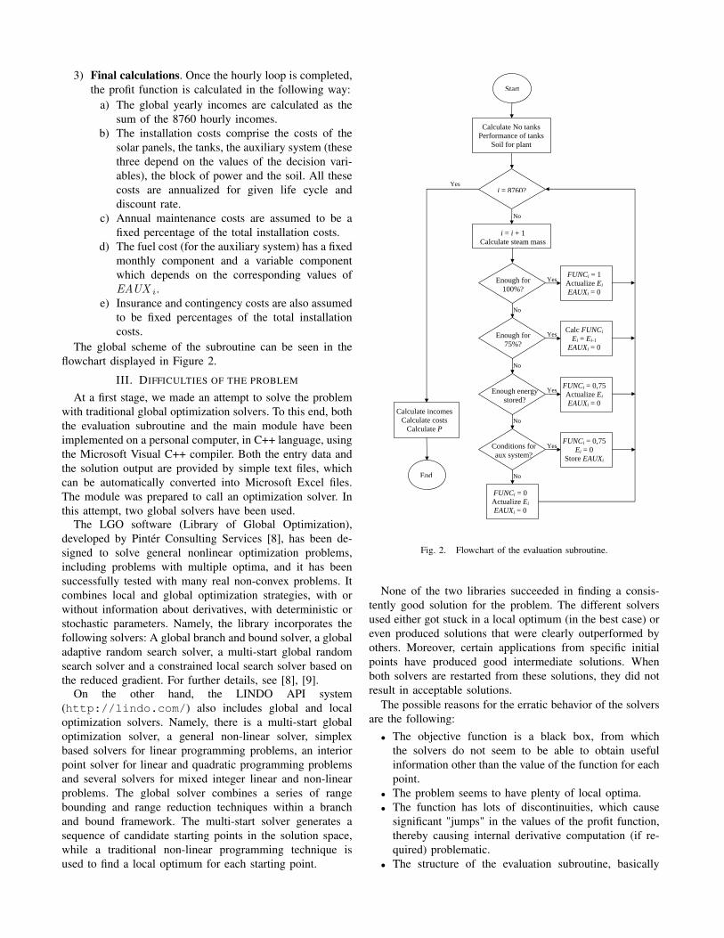
3) Final calculations. Once the hourly loop is completed,the profit function is calculated in the following way:

a) The global yearly incomes are calculated as thesum of the 8760 hourly incomes.

b) The installation costs comprise the costs of thesolar panels, the tanks, the auxiliary system (thesethree depend on the values of the decision vari-ables), the block of power and the soil. All thesecosts are annualized for given life cycle anddiscount rate.

c) Annual maintenance costs are assumed to be afixed percentage of the total installation costs.

d) The fuel cost (for the auxiliary system) has a fixedmonthly component and a variable componentwhich depends on the corresponding values ofEAUX i .

e) Insurance and contingency costs are also assumedto be fixed percentages of the total installationcosts.

The global scheme of the subroutine can be seen in theflowchart displayed in Figure 2.

III. DIFFICULTIES OF THE PROBLEM

At a first stage, we made an attempt to solve the problemwith traditional global optimization solvers. To this end, boththe evaluation subroutine and the main module have beenimplemented on a personal computer, in C++ language, usingthe Microsoft Visual C++ compiler. Both the entry data andthe solution output are provided by simple text files, whichcan be automatically converted into Microsoft Excel files.The module was prepared to call an optimization solver. Inthis attempt, two global solvers have been used.

The LGO software (Library of Global Optimization),developed by Pintér Consulting Services [8], has been de-signed to solve general nonlinear optimization problems,including problems with multiple optima, and it has beensuccessfully tested with many real non-convex problems. Itcombines local and global optimization strategies, with orwithout information about derivatives, with deterministic orstochastic parameters. Namely, the library incorporates thefollowing solvers: A global branch and bound solver, a globaladaptive random search solver, a multi-start global randomsearch solver and a constrained local search solver based onthe reduced gradient. For further details, see [8], [9].

On the other hand, the LINDO API system(http://lindo.com/) also includes global and localoptimization solvers. Namely, there is a multi-start globaloptimization solver, a general non-linear solver, simplexbased solvers for linear programming problems, an interiorpoint solver for linear and quadratic programming problemsand several solvers for mixed integer linear and non-linearproblems. The global solver combines a series of rangebounding and range reduction techniques within a branchand bound framework. The multi-start solver generates asequence of candidate starting points in the solution space,while a traditional non-linear programming technique isused to find a local optimum for each starting point.

Start

Calculate No tanks Performance of tanks

Soil for plant

i = 8760?

i = i + 1 Calculate steam mass

Enough for 100%?

Enough for 75%?

Enough energy stored?

Conditions for aux system?

FUNCi = 0 Actualize EiEAUXi = 0

FUNCi = 0,75 Ei = 0

Store EAUXi

FUNCi = 0,75 Actualize EiEAUXi = 0

Calc FUNCiEi = Ei-1

EAUXi = 0

FUNCi = 1 Actualize EiEAUXi = 0

Calculate incomes Calculate costs

Calculate P

End

Yes

No

Yes

No

Yes

No

Yes

No

Yes

No

Fig. 2. Flowchart of the evaluation subroutine.

None of the two libraries succeeded in finding a consis-tently good solution for the problem. The different solversused either got stuck in a local optimum (in the best case) oreven produced solutions that were clearly outperformed byothers. Moreover, certain applications from specific initialpoints have produced good intermediate solutions. Whenboth solvers are restarted from these solutions, they did notresult in acceptable solutions.

The possible reasons for the erratic behavior of the solversare the following:• The objective function is a black box, from which

the solvers do not seem to be able to obtain usefulinformation other than the value of the function for eachpoint.

• The problem seems to have plenty of local optima.• The function has lots of discontinuities, which cause

significant "jumps" in the values of the profit function,thereby causing internal derivative computation (if re-quired) problematic.

• The structure of the evaluation subroutine, basically

consisting on nested if-then commands results in a noisybehavior that misleads the solvers.

• Variables take widely different ranges of values, therebymaking it difficult for the solvers to provide adequateemphasis to correct variable combinations. For the sim-plex search, this may come from the generation of askewed (with a large aspect ratio) simplex.

In order to get an idea of the difficulty of the functionlandscape, we have created five sets of 10,000 random pointsand evaluated them. Table III presents the best solution andits function value among each one of these five sets. Thebest solutions are quite different from each other, therebyproviding no clue about the possible good search regions inthis problem.

TABLE IIICOMPARISON OF GA-OPTIMIZED SOLUTION WITH FIVE SETS OF

RANDOMLY CREATED SOLUTIONS.

Set P (x) x(e) AC (m2) E (kJ) Paux (kW)

1 27049676 693450 5405000000 1743002 23514158 594975 2492000000 2681003 22306797 655575 4981000000 5353004 22996207 688200 2478000000 3123005 28176740 712125 6490000000 98010

To get a more specific idea of the nature of the objectivefunction, we compute the objective function for severalvalues of the variable (AC) in the range [700,000, 750,000]m2 at a step of 10 m2 and keep E = 6, 346, 926, 197.10kJ and PAUX = 92, 768.3 kW (which, as we will see later,are their optimal values). This produces 5,001 solutions intotal. Figure 3 shows the variation of objective values withAC in the above range. The inset figure clearly shows thatthe function has many local optimum and is also too noisyto compute gradients properly by using any computationalmethod.

A_C

2.8e+07

2.82e+07

2.84e+07

2.86e+07

2.88e+07

2.9e+07

2.92e+07

2.94e+07

2.96e+07

700000 710000 720000 730000 740000 750000

Obje

ctiv

e V

alue

A_C (m^2)

2.82e+07

2.822e+07

2.824e+07

2.826e+07

2.828e+07

2.83e+07

2.832e+07

2.834e+07

710000 710500 711000 711500 712000 712500 713000 713500 714000

Ob

j. v

alu

e

2.78e+07

Fig. 3. Profit function variation with AC reveals multi-modality, noise andjumps in the objective function (E = 6, 346, 926, 197, PAUX = 92, 768).

IV. GENETIC ALGORITHM AS AN OPTIMIZATION TOOL

Genetic algorithms (GAs) are population based optimiza-tion algorithms which do not use any gradient information[4], [6]. While dealing with practical problems having dif-ferent complexities, such as noise, multimodality, numericalscaling of variables and others, many of which are prevalentto this problem, GAs have demonstrated their usefulness inthe past. First, we apply a standard GA to the solar thermalelectricity plant optimization problem and then discuss amodified approach.

A. A Standard GA

All variables of this problem are real-valued, thuswe use a real-coded GA (RGA) for this problem. AC-code implementing RGA is available from websitehttp://www.iitk.ac.in/kangal/soft.htm andis used here. The solution evaluation code supplied by theorganization is compiled and linked with the compiled RGAcode in a linux operating system. For evaluating a solution x,RGA sends the variable vector to the evaluation code whichthen returns the function value, P (x), of the supplied solutionvector. Figure 4 shows a schematic diagram of the linkingprocedure of RGA with the solution evaluator. Starting witha set of population members, RGA works in iteration bycreating new solutions which get evaluated by the solutionevaluator. The optimized solution is then printed.

Optimization

Evaluator

SolutionInit

ial

po

pu

lati

on

Algorithms

Geneticx

P(x)

x*, P(x*)

Fig. 4. The linking of an existing GA code with a solution evaluator.

RGA uses binary tournament selection, simulated binarycrossover (SBX) [2], and a polynomial mutation operator [1].A population of size 50, a crossover probability of 0.9 withSBX index of 2, a mutation probability of 1/3 with index 10are chosen. The GA is run for 150 generations. These arestandard values suggested in previous studies. To initializethe GA population, we use the following artificial upperbound for variables E and PAUX : E ≤ 1020, PAUX ≤ 1020.We obtain the following solution (x = (AC , E, PAUX )T ):

AC = 749, 980.86 m2, E = 6, 191, 823, 943.05 kJ,PAUX = 92, 898.24 kW, P (x) = 29, 189, 994.89 e.

First of all, we observe that our chosen artificial upper boundson E and PAUX did not influence the obtained solution. Sec-ondly, the optimized value of Ac is very close to the suppliedupper bound of 750, 000 m2. Thus, if this upper bound can

be increased, a better objective value is expected. Figure 5shows how the population best and average objective valuesimprove with generation number. The initial population best

Best

−1e+20

−8e+19

−6e+19

−4e+19

−2e+19

0

2e+19

0 20 40 60 80 100 120 140

Obje

ctiv

e V

alue

Generation Number

BestAverage

2.917e+07

2.9175e+07

2.918e+07

2.9185e+07

2.919e+07

2.9195e+07

80 90 100 110 120 130 140 150

Obje

ctiv

e V

alue

Generation Number

Fig. 5. Population best and average objective function values withgeneration number.

solution has an objective value −4.9106e19 (a negative profitdue to income (I) being smaller than cost (C)). At generation56, the population-best solution becomes positive for the firsttime, and then keeps on improving with generation beforestabilizing to its converged value 2.9189e07. Thus, the GA isable to make a significant progress from a very large negativevalue to a very high positive value in a span of only about120 generations. The inset plot in Figure 5 shows the detailedprogress of the algorithm after the 80-th generation. GAseems to progress steadily with generation finally reachingthe optimized value at generation 138. Note that the GA tooka total of 50 × 150 or 7, 500 solution evaluations. It is alsointeresting to note that the solution obtained by GA with7,500 solution evaluations is better than the best solutionfound by a random selection of 10,000 solutions, as reportedin Table III.

From the GA-optimized solution, we make another in-teresting observation. Each variable takes quite a differentorder of magnitude. The supplied and chosen variable boundswere quite large, thereby making any optimization algorithmdifficult to focus near the true optimum in this problem. Tomake the search more focused, we propose a modified GAwith a continuously updated variable bound scheme.

B. A Continuously Updated Genetic Algorithm

In the modified GA, we run the above GA for 150generations and note the best solution (say x∗) found thusfar. For each variable xi, the population standard deviationσi is computed. Thereafter, for the next 50 generations (wecall an epoch) we update the variable bounds as follows:

x(L)i = x∗i − σi, (2)

x(U)i = x∗i + σi. (3)

All the existing population members which are within theabove variable bounds are accepted in the new population.The remaining population slots are filled by creating randomsolutions within the above variable bounds. This procedureis continued for every 50 generations until there is nodifference in the best solutions of two consecutive epochs.This continuously updated variable bound procedure willallow a focused search and will allow the modified GA toconverge to a solution with generations.

We use identical GA parameter values as before. Theproposed GA runs for 650 generations before converging tothe following solution:

AC = 749, 999.99 m2, E = 6, 346, 926, 947.98 kJ,PAUX = 92, 768.27 kW, P (x) = 29, 201, 019.61 e.

This solution is slightly better (about 0.04%) than thatobtained by our previous GA. The variable AC reaches veryclose to its specified upper bound and other two variablevalues are also close to that found by previous GA procedure.Figure 6 shows the population best and average functionvalue with generation. Since the range of objective valuesfrom initial generation to final generation is quite significant,the progress of the algorithm is not comprehensible from theoverall plot. The inset figure shows the function values aftergeneration 100 and the steady progress of the algorithm isclear from the figure.

650

2e+19

0

−2e+19

−4e+19

−6e+19

−8e+19

−1e+200 150 200 250 300 350 400 450 500 550 600

150 200 250 300 350 400 450 500 550 600 650 2.91e+07

2.912e+07

2.914e+07

2.916e+07

2.918e+07

2.92e+07

Best

Best

Generation Number

Ob

ject

ive

Val

ue

Obje

ctiv

e V

alue

Generation Number

Average

Fig. 6. Population best and average objective function values withgeneration number for the modified GA.

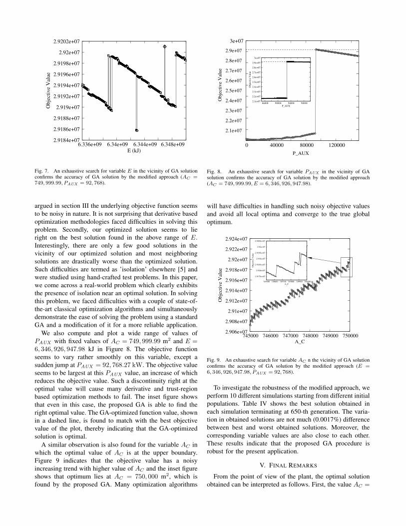
To investigate the accuracy of this optimized solutionand to support its probable optimality, we compute thesolutions in the vicinity of the optimized solution. For ananalysis for the variable E, we fix AC = 749, 999.99m2 and PAUX = 92, 768 kW in their optimized valuesand vary E in [6.335e9, 6.350e9] kJ with an increment of1000 kJ. This range is chosen around the optimized valueof E. This resulted in 10,000 solutions and we plot thecorresponding objective values in Figure 7. There are twodistinct facts to be observed from this figure. First, theobjective function seems to be quite sensitive to E and as

E (kJ)

2.9186e+07

2.9188e+07

2.919e+07

2.9192e+07

2.9194e+07

2.9196e+07

2.9198e+07

2.92e+07

2.9202e+07

6.336e+09 6.34e+09 6.344e+09 6.348e+09

Obje

ctiv

e V

alue

2.9184e+07

Fig. 7. An exhaustive search for variable E in the vicinity of GA solutionconfirms the accuracy of GA solution by the modified approach (AC =749, 999.99, PAUX = 92, 768).

argued in section III the underlying objective function seemsto be noisy in nature. It is not surprising that derivative basedoptimization methodologies faced difficulties in solving thisproblem. Secondly, our optimized solution seems to lieright on the best solution found in the above range of E.Interestingly, there are only a few good solutions in thevicinity of our optimized solution and most neighboringsolutions are drastically worse than the optimized solution.Such difficulties are termed as ’isolation’ elsewhere [5] andwere studied using hand-crafted test problems. In this paper,we come across a real-world problem which clearly exhibitsthe presence of isolation near an optimal solution. In solvingthis problem, we faced difficulties with a couple of state-of-the-art classical optimization algorithms and simultaneouslydemonstrate the ease of solving the problem using a standardGA and a modification of it for a more reliable application.

We also compute and plot a wide range of values ofPAUX with fixed values of AC = 749, 999.99 m2 and E =6, 346, 926, 947.98 kJ in Figure 8. The objective functionseems to vary rather smoothly on this variable, except asudden jump at PAUX = 92, 768.27 kW. The objective valueseems to be largest at this PAUX value, an increase of whichreduces the objective value. Such a discontinuity right at theoptimal value will cause many derivative and trust-regionbased optimization methods to fail. The inset figure showsthat even in this case, the proposed GA is able to find theright optimal value. The GA-optimized function value, shownin a dashed line, is found to match with the best objectivevalue of the plot, thereby indicating that the GA-optimizedsolution is optimal.

A similar observation is also found for the variable AC inwhich the optimal value of AC is at the upper boundary.Figure 9 indicates that the objective value has a noisyincreasing trend with higher value of AC and the inset figureshows that optimum lies at AC = 750, 000 m2, which isfound by the proposed GA. Many optimization algorithms

P_AUX

80000 40000 0

3e+07

2.1e+07

2.2e+07

2.3e+07

2.4e+07

2.5e+07

2.6e+07

2.7e+07

2.8e+07

2.9e+07

P_AUX

Obje

ctiv

e V

alue

2.1e+07

2.2e+07

2.3e+07

2.4e+07

2.5e+07

2.6e+07

2.7e+07

2.8e+07

2.9e+07

3e+07

86000 90000 94000 98000

Obje

ctiv

e V

alue

120000

Fig. 8. An exhaustive search for variable PAUX in the vicinity of GAsolution confirms the accuracy of GA solution by the modified approach(AC = 749, 999.99, E = 6, 346, 926, 947.98).

will have difficulties in handling such noisy objective valuesand avoid all local optima and converge to the true globaloptimum.

A_C

2.908e+07

2.91e+07

2.912e+07

2.914e+07

2.916e+07

2.918e+07

2.92e+07

2.922e+07

2.924e+07

745000 746000 747000 748000 749000 750000

Ob

ject

ive

Val

ue

A_C

2.9175e+07

2.918e+07

2.9185e+07

2.919e+07

2.9195e+07

2.92e+07

2.9205e+07

749500 749600 749700 749800 749900 750000

Ob

ject

ive

Val

ue

2.906e+07

Fig. 9. An exhaustive search for variable AC n the vicinity of GA solutionconfirms the accuracy of GA solution by the modified approach (E =6, 346, 926, 947.98, PAUX = 92, 768).

To investigate the robustness of the modified approach, weperform 10 different simulations starting from different initialpopulations. Table IV shows the best solution obtained ineach simulation terminating at 650-th generation. The varia-tion in obtained solutions are not much (0.0017%) differencebetween best and worst obtained solutions. Moreover, thecorresponding variable values are also close to each other.These results indicate that the proposed GA procedure isrobust for the present application.

V. FINAL REMARKS

From the point of view of the plant, the optimal solutionobtained can be interpreted as follows. First, the value AC =

TABLE IVBEST SOLUTION OBTAINED IN 10 RUNS OF MODIFIED GA APPROACH.

P (x∗) x∗

(e) AC (m2) E (kJ) PAUX (kW)29201019.61 749999.99 6346926947.98 92768.2729201018.75 749999.94 6346929408.75 92768.2629201018.62 749999.94 6346929669.93 92768.2629201018.62 749999.94 6346929478.79 92768.2729200967.67 749997.61 6347055515.19 92768.4629200967.42 749997.62 6347055515.19 92768.4629200957.23 749997.01 6347087739.59 92768.2729200953.07 749997.00 6347092303.42 92768.3129200922.51 749999.96 6346929711.66 92777.4929200522.97 749992.62 6318673893.16 92768.70

750, 000 m2 is the bound imposed by the firm. In fact, inpreliminary studies where we did not establish this limit,the ideal area was around 950, 000 m2. Second, the valuePAUX = 92, 768.27 kW reflects the necessary power thatcan enable the plant to reach 75% of its full production, usingexclusively the auxiliary system. Finally, the total storagecapacity would be one full tank and around 90% of thesecond one. There are also two other remarkable data inthe optimal solution. The sum over the whole year of thevariables FUNC i equals 5,413.70 hours. This means thatthe plant is working 61.80% out of the 8,760 hours of theyear. The final value PERC 8760 is 15%, that is, the legalhybridization limit is reached at the end of the year.

Having solved the problem using GAs and then providingjustification for the optimality of the obtained solution,we have now understood various challenges provided bythe three-variable optimization problem of sizing the solarthermal electricity plant. We outline them in the following:

• The objective function is noisy.• The objective function has massive multimodality.• The objective function has discontinuities.• The optimal solution lies on a discontinuous point in

the search space.• The optimal solution lies on a variable boundary.• The optimal solution is isolated and is surrounded by

not-so-good solutions, resembling a local needle-in-haystack problem.

• The optimal decision variable values are of differentorders of magnitude with a maximum difference of fiveorders of magnitude.

Any of the above challenges is difficult for most derivativeand classical optimization methods. The combination of thesechallenges is even worse. The flexibility and global searchperspective of GAs make them suitable for solving suchproblems. Finally, this problem indicates that a small sizedproblem (with only three variables in this problem) need notalways be termed as an easy problem for an optimizationalgorithm. The function landscape provides a true picture ofthe challenges offered by a problem.

VI. CONCLUSIONS

Many optimization studies demonstrated in the literatureusually involve smooth objective functions and well-scaledvariables. However, the practice is far from being so ideal.In this paper, we come across a three-variable maximizationproblem which exhibits common complexities which manyreal-world optimization problems possess. Some of thesedifficulties are (i) black-box optimization, (ii) noisy objectivefunction, (iii) massive multi-modality, (iv) non-uniform rangeof variable values, and (v) extremely wide range of searchregion. When attempted to solve using a couple of classicalgradient based optimization techniques, the effort resulted inno useful solution due to the inflexibilities involved with theclassical approaches in dealing with above difficulties.

On the contrary, with genetic algorithms, we have experi-enced a completely different outcome. A standard real-codedGA, starting from not-so-good initial random solutions, hasbeen able to progress close to reasonably good solutionsquickly by negotiating all the above difficulties. To make theperformance better, we have also suggested a modified GAwith a continuously updated search procedure. An analysisof solutions around the vicinity of the obtained solution hassupported the optimality of the obtained solution.

This study clearly demonstrates the usefulness of geneticalgorithms in practical optimization and flexibility of han-dling different vagaries of problem difficulties which oftenarise in applied optimization problems.

ACKNOWLEDGMENTS

This work has been done in the frame of the joint project"GDV-500 Plus" with the firm Endesa Generación S.L.

J.M. Cabello, M. Luque and F. Ruiz acknowledge thesupport from the Spanish Ministry of Education and Science(Research Project MTM2006-01921), and from the Andalu-sian Regional Ministry of Innovation, Science and Enterprise(PAI group SEJ-445).

K. Deb and R. Tewari acknowledge the support fromAcademy of Finland and the Foundation of Helsinki Schoolof Economics.

REFERENCES

[1] K. Deb. Multi-objective optimization using evolutionary algorithms.Chichester, UK: Wiley, 2001.

[2] K. Deb and R. B. Agrawal. Simulated binary crossover for continuoussearch space. Complex Systems, 9(2):115–148, 1995.

[3] R. D. Doering and B. W. Lin. Optimum operation of a total energyplant. Computers and Operations Research, 6(1):33–38, 1979.

[4] D. E. Goldberg. Genetic Algorithms for Search, Optimization, andMachine Learning. Reading, MA: Addison-Wesley, 1989.

[5] D. E. Goldberg. The design of innovation: Lessons from and forCompetent genetic algorithms. Kluwer Academic Publishers, 2002.

[6] J. H. Holland. Adaptation in Natural and Artificial Systems. AnnArbor, MI: MIT Press, 1975.

[7] D. Mills. Advances in solar thermal electricity technology. SolarEnergy, 76:19–31, 2004.

[8] J. D. Pinter. Computational Global Optimization in Nonlinear Systems.An Interactive Tutorial. Lionheart Publishing, Inc., Atlanta, GA, 2001.

[9] J. D. Pinter. Nonlinear Optimization with MPL/LGO: Introduction andUser’s Guide. Maximal Software, 2006.

[10] C. Triki, P. Beraldi, and G. Gross. Optimal capacity allocation inmulti-auction electricity markets under uncertainty. Computers andOperations Research, 32(2):201–217, 2005.