optimization of the production of long-chain dicarboxylic
TRANSCRIPT

Rose-Hulman Institute of TechnologyRose-Hulman Scholar
Graduate Theses - Chemical Engineering Graduate Theses
Summer 8-2018
Optimization of the Production of Long-ChainDicarboxylic Acids from Distillers Corn Oil UsingCandida viswanathiiJennifer Ann MobleyRose-Hulman Institute of Technology
Follow this and additional works at: https://scholar.rose-hulman.edu/chemical_engineering_grad_theses
This Thesis is brought to you for free and open access by the Graduate Theses at Rose-Hulman Scholar. It has been accepted for inclusion in GraduateTheses - Chemical Engineering by an authorized administrator of Rose-Hulman Scholar. For more information, please contact [email protected].
Recommended CitationMobley, Jennifer Ann, "Optimization of the Production of Long-Chain Dicarboxylic Acids from Distillers Corn Oil Using Candidaviswanathii" (2018). Graduate Theses - Chemical Engineering. 11.https://scholar.rose-hulman.edu/chemical_engineering_grad_theses/11
Optimization of the Production of Long-Chain Dicarboxylic Acids from Distillers Corn Oil
Using Candida viswanathii
A Thesis
Submitted to the Faculty
of
Rose-Hulman Institute of Technology
by
Jennifer Ann Mobley
In Partial Fulfillment of the Requirements for the Degree
of
Master of Science in Chemical Engineering
August 2018
© 2018 Jennifer Ann Mobley


ABSTRACT
Mobley, Jennifer Ann
M.S.Ch.E.
Rose-Hulman Institute of Technology
August 2018
Optimization of the Production of Long-Chain Dicarboxylic Acids from Distillers Corn Oil
Using Candida viswanathii
Thesis Advisor: Dr. Irene Reizman
This thesis explores the viability of using the yeast Candida viswanathii to convert
distillers corn oil, a byproduct of the ethanol industry, into long-chain α,ω-dicarboxylic acids
used in lubricants, cosmetics, and biopolymers. Glucose, xylose, and glycerol were used as
carbon sources for the determination of growth parameters of this strain, of which it was found
that growth on glucose resulted in the highest specific growth rate of 0.482 hr-1 and the lowest
biomass yield coefficient of 0.566 - 0.754 g DCW per g substrate on average. A prior developed
analytical method for determining feed and product concentrations in fermentation broth using
gas chromatography was gradually improved throughout this study. However, it was found that
repeatability issues still occurred with the method. The production of diacids was studied with
different feedstocks and co-substrates, where it was found that diacid production occurred with
all combinations, except methyl oleate and glucose. It was observed that both methyl oleate and
oleic acid had solubility issues, which could be further improved within the fermentation broth.
Keywords: Chemical Engineering, Dicarboxylic Acid Production, Renewable Resources

ACKNOWLEDGEMENTS
First, I would like to thank my thesis advisor, Dr. Irene Reizman, for all of her help with
devising methods, troubleshooting, and pointing me towards the many resources that I used this
past year. I am very grateful for her dedication as an advisor, providing me with the opportunity
to present posters at two different conferences and helping me to contact many people from other
universities and companies that are researching in the same field. I would like to thank my
advisory committee, Dr. Mark Brandt and Dr. Coppinger, for all of the fun conversations and
other tips that they had for me throughout the project. The statistical analysis in this report could
not have been completed without insight from Dr. Eric Reyes, nor would I have gotten far with
the analytical methods if Dr. Dan Morris had not contributed some ideas for troubleshooting.
Regarding faculty, this project would not have been possible without Lou Johnson and Frank
Cunning and their endless support to make sure that the equipment I was using in the chemistry
and chemical engineering labs was in good condition. Regarding colleagues, I am thankful for
the contributions of Katie Ryan, Nick Palmer, Anna Defries, and Xin Tang for their side projects
in analytical methods, scale up and design, statistical modeling, and extraction optimization for
this research respectively. Lastly, I would like to thank my senior design teammates for helping
me to develop an interest in using corn as a renewable resource.
I am grateful to say that this research is funded by the Indiana Corn Marketing Council. I
am also proud to say that this research has the support of the National Corn Growers
Association, which awarded me 3rd place in their poster competition at the 2018 Corn Utilization
and Technology Conference.

ii
TABLE OF CONTENTS
LIST OF FIGURES ................................................................................................................ iv
LIST OF TABLES .................................................................................................................. ix
LIST OF ABBREVIATIONS ................................................................................................. xi
LIST OF SYMBOLS ............................................................................................................. xiii
1. INTRODUCTION ..............................................................................................................1
1.1 Project Impact on the Production of Specialty Chemicals from Renewable Resources ...1
1.2 Summary of Objectives .................................................................................................4
2. BACKGROUND ................................................................................................................7
2.1 Contemporary Production of LCDCAs in Industry and Academia .................................7
2.2 Justification for Using Distillers Corn Oil as a FFA Feedstock ......................................9
3. LITERATURE REVIEW ................................................................................................ 11
3.1 Exploration of Feedstocks and the Chain Lengths of DCAs from Biotransformations.. 11
3.2 Bioreactor and Shake Flask Conditions Tested for LCDCA Production ....................... 12
3.3 Growth of C. viswanathii and C. tropicalis on Common Carbon Substrates ................ 21
3.4 Analytical Methods for Quantifying LCDCAs in Fermentation Broth ......................... 24
3.5 Difficulties Encountered During Production and Analysis ........................................... 27
4. DESCRIPTION OF THE MODEL ................................................................................. 29
4.1 Derivation of the Growth Rate Model ......................................................................... 29
4.2 Derivation of the Substrate Consumption Model ......................................................... 30
4.3 Further Development of Models for Analysis in RStudio ............................................ 32
5. MATERIALS AND METHODS ..................................................................................... 38
5.1 Description of the Major Equipment Used................................................................... 38
5.1.1 YSI Bioanalyzer................................................................................................... 39
5.1.2 GC-MS ................................................................................................................ 40
5.1.3 HPLC .................................................................................................................. 41
5.2 Preparation of Cell Bank ............................................................................................. 42
5.3 Growth Study Method and Conditions ........................................................................ 42
5.3.1 YSI Bioanalyzer Setup and Calibration ................................................................ 44

iii
5.4 Production Study Method and Conditions ................................................................... 45
5.4.1 Original Extraction and Derivatization Method of Production Samples ................ 50
5.4.2 Gas Chromatography and Mass Spectrometry Parameters .................................... 51
5.4.3 High-Performance Liquid Chromatography (HPLC) Parameters .......................... 54
6. RESULTS ......................................................................................................................... 56
6.1 Growth Characterization of C. viswanathii .................................................................. 56
6.1.1 Specific Growth Rate ........................................................................................... 57
6.1.2 Biomass Yield Coefficient ................................................................................... 60
6.2 Analytical Method Development ................................................................................. 64
6.3 LCDCA Production Studies ........................................................................................ 79
7. DISCUSSION ................................................................................................................... 82
7.1 Optimal Carbon Substrate for Growth of C. viswanathii .............................................. 82
7.2 Analytical Method Improvements and Contributions to Literature ............................... 91
7.2.1 Alterations to the Extraction Protocol ................................................................... 91
7.2.2 Alterations to the Derivatization Protocol ............................................................. 92
7.2.3 Identification of the Unsaturated DCA Product with GC-MS ............................... 97
7.2.4 Implementation of Internal Standards ................................................................... 98
7.2.5 Adjustment of GC Injection Volume and Temperature ....................................... 100
7.3 Conditions for Relatively Highest LCDCA Yield ...................................................... 104
8. CONCLUSIONS AND FUTURE WORK..................................................................... 111
LIST OF REFERENCES ...................................................................................................... 114
APPENDICES ....................................................................................................................... 119
APPENDIX A ........................................................................................................................ 120
APPENDIX B ........................................................................................................................ 123
APPENDIX C ........................................................................................................................ 128
APPENDIX D ........................................................................................................................ 130
APPENDIX E ........................................................................................................................ 131

iv
LIST OF FIGURES
Figure Page
Figure 2.1.1: Summary of the ω-oxidation pathway present in the engineered E. coli used
by Sathesh-Prabu and Lee. The CYP450 is expected to be different for other
organisms, but has the same function14. ............................................................................7
Figure 3.3.1: The specific growth rate of C. tropicalis related to the xylose concentration via
the Monod equation in a simple medium without the sago trunk hydrolysate as found
by Mohamad et al.32. ........................................................................................................ 22
Figure 3.3.2: The production of dodecanedioic acid (A), biomass yield (B), and substrate
consumption (C) of sucrose, glucose, xylose, and arabinose with C. viswanathii as
investigated by Cao et al30. ............................................................................................... 23
Figure 3.5.1: The improved effects on productivity and activity of CYP450s in C. tropicalis
as found by Liu et al. The unfilled points represent the productivity measurements
and the filled points correspond to the activity of CYP450. Circles are used for the
devised pH strategy, while squares are used for a constant pH of 8. ............................. 28
Figure 5.4.1: C. viswanathii is plated on YPD agar to determine cell viability in the first
production study conducted. The dilutions of the samples from left to right are 1:100,
1:10,000, and 1:1,000,000. A simple circular and smooth morphology is observed...... 49
Figure 6.1.1.1: Raw data of C. viswanathii grown on various carbon substrates. ................. 57
Figure 6.1.1.2: Comparison of typical growth rates of C. viswanathii on the three separate
carbon sources. Glucose appears to have the highest specific growth rate in the
exponential term, followed by xylose and then glycerol. ................................................ 58
Figure 6.1.1.3 : Growth study data overlaid with the nonlinear mixed effects model derived
and fit in RStudio. The specific growth rate on glycerol appears to be much smaller
than the other substrates. The mixtures containing glucose and the pure glucose
substrate have the highest values, however, the curves are not overlaid as they would
be if they had identical specific growth rates. ................................................................. 59
Figure 6.1.2.1: Raw data of the substrate consumption of C. viswanathii on various
substrates. ......................................................................................................................... 61

v
Figure 6.1.2.2: Characteristic substrate consumption curves for each type of carbon
substrate. .......................................................................................................................... 61
Figure 6.1.2.3: Substrate consumption rate data overlaid with the nonlinear mixed effects
model derived and fit in RStudio. It appears that growth on glucose mixed with
glycerol has the highest biomass yield coefficient and glycerol has the lowest by a large
degree................................................................................................................................ 62
Figure 6.2.1: Illustration of how the calibration curve determined for methyl oleate
changed by 72% based off of the change in slope when the extraction step was
included. This is assumed to be equal to the yield of the extraction, where another
method of determining minimum yield is to compare the points of the highest
concentration standard, which comes out to a difference of 71%. ................................. 65
Figure 6.2.2: Repeatability issues are illustrated with the injection volume by how methyl
oleate standards at four different concentrations either exhibited a high or low value
for the peak integration when tested three times each. The actual injection volumes
are unknown, but the parameter was kept constant at 5 µL. ......................................... 66
Figure 6.2.3: The inconsistency in the injection volume is clearly illustrated where a single
sample was tested four times, and for each component there was an upper and lower
bound. Minimal scatter is observed. MO is methyl oleate, LAME, is linoleic acid
methyl ester, SAME is stearic acid methyl ester, and the MO isomer is an unidentified
compound that forms a doublet peak with MO in the technical grade solution. ........... 66
Figure 6.2.4: By doubling the amount of MSTFA added, which was already in excess, the
calibration curve for oleic acid improved significantly and there was less scatter in the
data. This improvement was observed for both internal standards used in the study. 67
Figure 6.2.5: By doubling the amount of MSTFA added, which was already in excess, the
calibration curve for C18 DCA improved so that there was more of a substantial slope
in the calibration curve. This improvement was observed for both internal standards
used in the study. The data points for the highest concentration of C18 DCA for the
50µL trials are not included since no peaks appeared in the resulting chromatographs.
.......................................................................................................................................... 68
Figure 6.2.6: By increasing the ratio of MSTFA to pyridine from 4:1 (12.5 µL of pyridine)
to 6:1 (8.33 µL of pyridine), there appeared to be no significant difference besides a
slight increase in slope, representing a slightly heightened sensitivity. .......................... 68
Figure 6.2.7: Decreasing the derivatization time at 60°C improves the sensitivity of the
calibration curve significantly, while longer time periods appear to break down the
components since only one concentration was detectable for the 40 minute and 60
minute samples. ................................................................................................................ 69

vi
Figure 6.2.8: Calculations done on the solvent expansion calculator by Restek to show that
the maximum injection volume to prevent excessive back flash is 2.2 µL as shown in
(B), but the 5 µL injection volume used previously produces a vapor cloud double the
size of the volume of the liner as shown in (A)53.............................................................. 70
Figure 6.2.9: GC-MS chromatograph representing a production trial sample that is
expected to have oleic acid (OA) in it. The internal standards at 11.3 min (PME) and
15.4 min (HME) are barely present, indicating that either the injection volume or
injection temperature was too low. The injection temperature set was the original
value of 275°C. ................................................................................................................. 71
Figure 6.2.10: The same sample in Figure 6.2.9 was tested again at 300°C twice and found
to have the oleic acid peak appear at 18.9 min. However, it is clear that in trial (A)
there was a little bit of C18:0 DCA present at 26.4 min but not in trial (B). Trial (B)
also has a much cleaner baseline. .................................................................................... 72
Figure 6.2.11: Example of a high-resolution chromatograph using an injection temperature
of 300°C to study an unknown with oleic acid and C18:1 and C18:0 DCAs present with
a trace amount of stearic acid. ......................................................................................... 73
Figure 6.2.12: Example of a chromatograph of an unknown studied at an injection
temperature of 300°C that has random artifact peaks that are not usually seen between
12.5 min and 13.5 min. They are most likely degradation products of the TMS
derivatives or methyl oleate. ............................................................................................ 73
Figure 6.2.13: Example of a chromatograph of an unknown studied at an injection
temperature of 300°C that has artifact peaks that occasionally occur around 20.0 min
and 23.3 min. They are most likely degradation products of the C18:0 and C18:1 DCA
TMS derivatives due to their higher retention time and boiling point. ......................... 74
Figure 6.2.14: Example of a chromatograph of a standard containing technical grade
methyl oleate and oleic acid studied at an injection temperature of 275°C. An artifact
peak that regularly occurs when oleic acid standards are derivatized is present at 26.4
min. This overlaps with the retention time for C18:0 DCA, indicating that it may not
be an artifact at all but the presence of DCA that was still stuck on the column. ......... 74
Figure 6.2.15: Example of how the new analytical method can give high resolution for the
four main components of interest with a standard comprising of from left to right: 0.5
g/L PME, 0.5 g/L HME, 1 g/L methyl oleate (MO), 1 g/L oleic acid (OA), 1 g/L stearic
acid (SA), and 1 g/L C18:0 DCA...................................................................................... 75
Figure 6.2.16: A zoomed in picture of a chromatograph with the newly discovered peaks
from using the new method. With the mass spectrum shown, it is thought that the first
peak is most likely C18:1 DCA. ....................................................................................... 76

vii
Figure 6.2.17: A mass spectrum for C18:1 DCA as found by Judefeind et al.36. .................. 76
Figure 6.2.18: Calibration curves for methyl oleate using both internal standards, PME
and HME. ......................................................................................................................... 77
Figure 6.2.19: Calibration curves for oleic acid using both internal standards, PME and
HME. ................................................................................................................................ 77
Figure 6.2.20: Calibration curves for stearic acid using both internal standards, PME and
HME. ................................................................................................................................ 78
Figure 6.2.21: Calibration curves for C18:0 DCA using both internal standards, PME and
HME. ................................................................................................................................ 78
Figure 6.3.1: The change in concentration of four key components over time measured by
GC-MS in Flask RCA, which was given 10 g/L of glucose for the co-substrate and no
feedstock. At 24 hours, there appears to be a considerable amount of DCA produced,
but this trend was observed for all samples tested that day, indicating a possible issue
with standard carryover. ................................................................................................. 79
Figure 6.3.2: The change in concentration of four key components over time measured with
GC-MS in Flask R2A, which was given 10 g/L of methyl oleate as feedstock and 10 g/L
of glucose for the co-substrate. There appears to be an increase in methyl oleate
concentration after 48 hours, indicating possible solubility issues. ................................ 80
Figure 6.3.3: The change in concentration of four key components over time measured with
GC-MS in Flask R3A, which was given 10 g/L of methyl oleate as feedstock and 10 g/L
of glucose for the co-substrate. There appears to be a large discrepancy in the oleic
acid concentration at the end of the study, where running the sample twice on the GC
produced very different results. ...................................................................................... 80
Figure 6.3.4: The change in concentration of four key components over time measured by
HPLC in Flask R2A, which was given 10 g/L of methyl oleate as feedstock and 25 g/L
of glucose for the co-substrate. Samples at all time periods were tested once with a
refractive index and an absorbance measurement. There still appears to be an
increase in methyl oleate concentration at 48 hours, and there is no product formed
throughout the trial. ......................................................................................................... 81
Figure 6.3.5: The change in concentration of four key components over time measured with
GC-MS in Flask R3A, which was given 10 g/L of methyl oleate as feedstock and 10 g/L
of glucose for the co-substrate. Samples at all time periods were tested once with a
refractive index and an absorbance measurement. There appears to be no consistent
consumption of methyl oleate and no product formed throughout the trial. There is a
slight discrepancy in the oleic acid concentration at 120 hours. .................................... 81

viii
Figure 7.1.1: Growth curves of C. viswanathii studied on 4/18/18 in the spring quarter with
glucose or a glucose and xylose mixture for the carbon substrate. ................................ 89
Figure 7.1.2: Growth curves of C. viswanathii studied on 4/11/18 in the spring quarter with
a glucose and glycerol mixture or a glucose and xylose mixture for the carbon
substrate. .......................................................................................................................... 89
Figure E.1: Calibration curve relating optical density (OD600) to dry cell weight
concentration. ................................................................................................................. 131

ix
LIST OF TABLES
Table Page
Table 2.2.1: Composition of thin stillage, stored at room temperature, as characterized by
Winkler-Moser et al26....................................................................................................... 10
Table 3.2.1: Summary of the medium composition used for the production of LCDCAs in
the study by Cao et al.30 ................................................................................................... 13
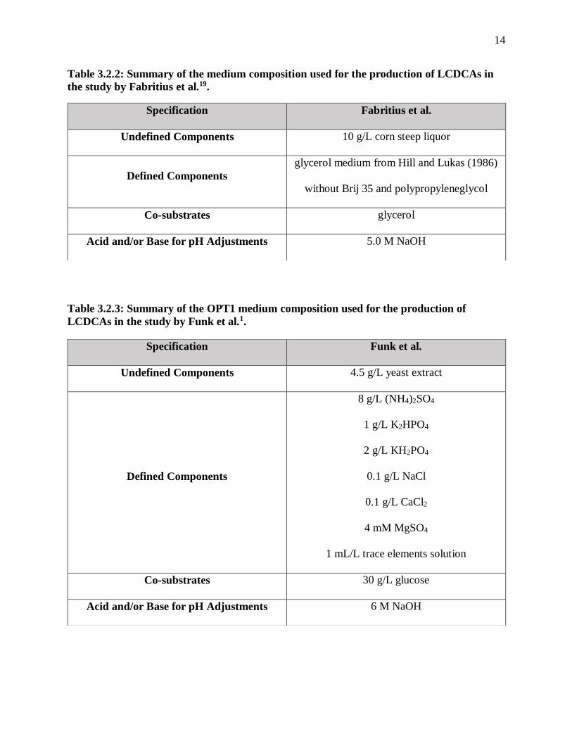
Table 3.2.2: Summary of the medium composition used for the production of LCDCAs in
the study by Fabritius et al.19. .......................................................................................... 14
Table 3.2.3: Summary of the OPT1 medium composition used for the production of
LCDCAs in the study by Funk et al.1. ............................................................................. 14
Table 3.2.4: Summary of the medium composition used for the production of LCDCAs in
the study by Liu et al.20. ................................................................................................... 15
Table 3.2.5: Summary of the medium composition used for the production of LCDCAs in
the study by Mobley11. ..................................................................................................... 16
Table 3.2.6: Summary of the medium composition used for the production of LCDCAs in
the study by Picataggio et al.16. ........................................................................................ 16
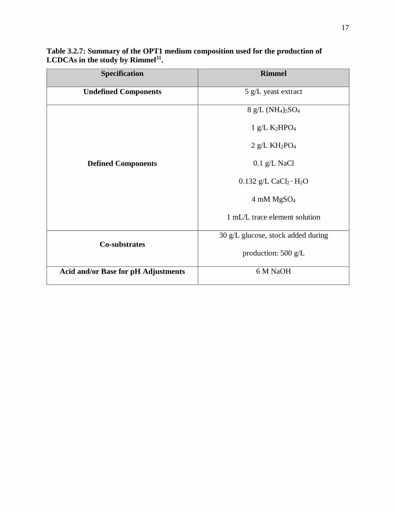
Table 3.2.7: Summary of the OPT1 medium composition used for the production of
LCDCAs in the study by Rimmel31. ................................................................................ 17
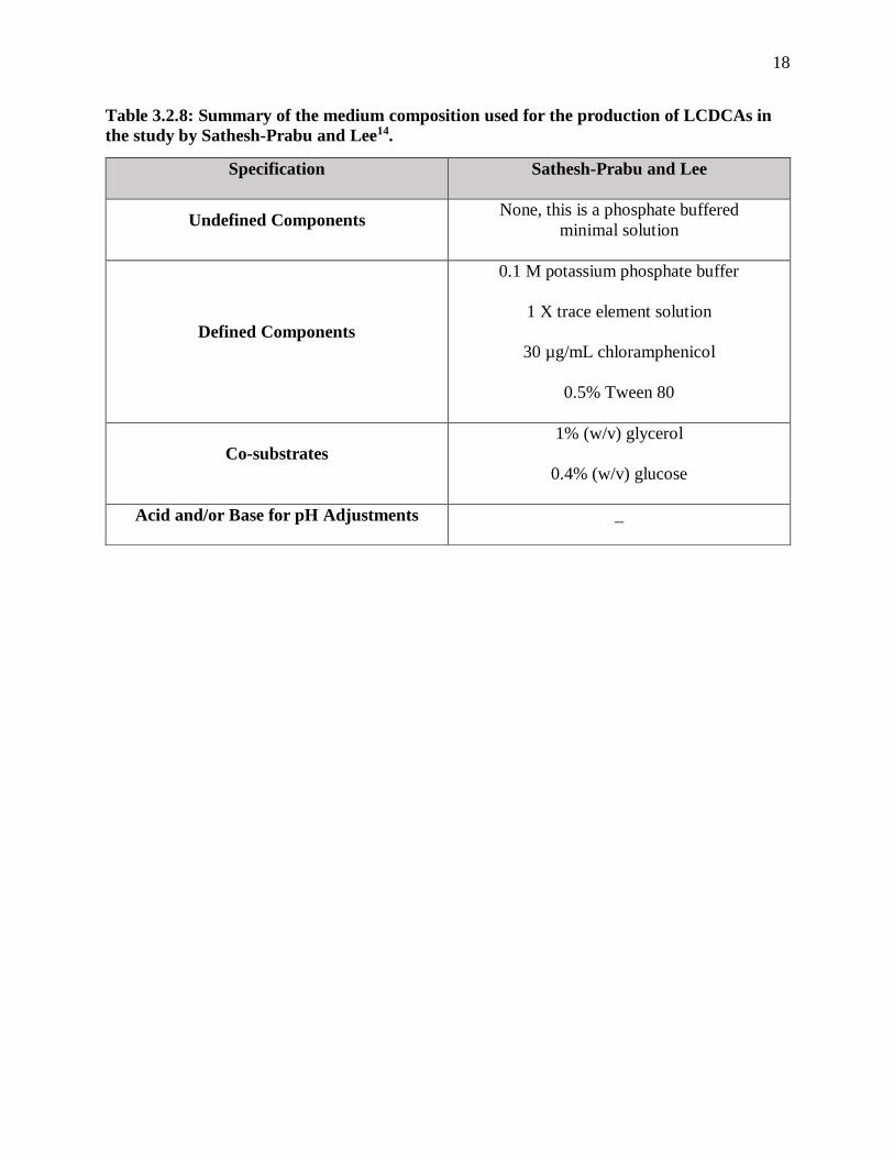
Table 3.2.8: Summary of the medium composition used for the production of LCDCAs in
the study by Sathesh-Prabu and Lee14. ........................................................................... 18
Table 3.2.9: Summary of the broth conditions used for the production of LCDCAs in the
most referenced literature sources1,11,14,16,19,20,30,31. Modified yeast strains were used in
each study, except Sathesh-Prabu and Lee used E. coli.................................................. 19
Table 3.2.10: Comparison of C12 DCA titers between the studies of Picataggio et al.,
Sathesh-Prabu et al., Cao et al., and others as presented by Cao et al.30. ...................... 20
Table 3.4.1: Summary of the gas chromatography specifications highlighted in the reports
of Funk et al., Rimmel, and Sathesh-Prabu and Lee1,14,31. ............................................. 26
x
Table 5.1.1.1: List of materials and parameters for all membrane configurations to
determine substrate concentration on the YSI 2900 Bioanalyzer41. ............................... 40
Table 5.4.1: List of experimental conditions for all trials conducted in the production of
LCDCAs with C. viswanathii. .......................................................................................... 47
Table 5.4.2.1: Summary of the parameters set for the gas chromatography column, after
the modifications made in this study. .............................................................................. 53
Table 5.4.2.2: Summary of the parameters set for the mass spectrometry data collection. . 54
Table 6.1.1: Summary of the trials conducted for the C. viswanathii growth study. ............ 56
Table 6.1.1.1: Summary of the specific growth rates found for each substrate combination
and the hypothesis testing conducted to determine if the specific growth rates differed
significantly from glucose. ............................................................................................... 59
Table 6.1.2.1: Summary of the values for the biomass yield coefficient on each substrate
determined by both statistical modeling and numerical calculations. ........................... 63
Table 7.2.1: Summary of all of the changes made in the analytical method for the
determination of FFA and DCA concentrations with GC-MS. .................................... 103
Table 7.3.1: Observational summary of the data collected using HPLC for select cultures
grown with the following trial conditions. All conditions resulted in the production of
C18:1 DCA except for the trials involving glucose and methyl oleate. There were no
consistent trends for the consumption of the feedstock in any of the trials. ................ 108
Table A.1: Recipe for YPD agar plates used to isolate colonies of C. viswanathii and
determine cell viability. .................................................................................................. 120
Table A.2: Recipe for OPT1 media used in growth and production studies....................... 121
Table A.3: Recipe for the trace element solution used in the growth and production studies.
........................................................................................................................................ 122
Table C.1: List of the chemicals used in the aforementioned experiments, excluding those
needed to operate the YSI 2900 Bioanalyzer. ................................................................ 128

xi
LIST OF ABBREVIATIONS
ATCC American Type Culture Collection
C. viswanathii
C. tropicalis
Candida viswanathii
Candida tropicalis
CXX:Y
Indicates that the molecule has XX
carbons in a chain and has Y degrees
of unsaturation or carbon-carbon
double bonds
DAD Diode Array Detector
DCA Dicarboxylic acid(s)
DCO Distillers Corn Oil
DCW Dry Cell Weight
DDGS Distillers Dried Grains with Solubles
FFA Free Fatty Acid(s)
FID Flame Ionization Detector
GC Gas Chromatography
HME Methyl Heptadecanoate
HPLC High Performance Liquid
Chromatography
IS Internal Standard
LCDCA Long-Chain Dicarboxylic Acid(s)
MO Methyl Oleate
MS Mass Spectrometry

xii
MSTFA N-Methyl-N-(trimethylsilyl)
trifluoroacetamide
MTBE Tert-Butyl Methyl Ether
NIST National Institute of Standards and
Technology
OA Oleic Acid
OD Optical Density
PME Methyl Pentadecanoate
RID Refractive Index Detector
SIM Selective Ion Monitoring
TMS Trimethylsilyl (derivative)
UV-Vis Ultraviolet and Visible Light
xg Times Gravity, 9.81 m2/s, to denote
amount of centrifugal force

xiii
LIST OF SYMBOLS
English Symbols
𝑚 Maintenance coefficient 𝑔 𝑠𝑢𝑏𝑠𝑡𝑟𝑎𝑡𝑒
𝑔 𝑏𝑖𝑜𝑚𝑎𝑠𝑠 ∙ ℎ𝑟
𝑃 Product concentration 𝑔/𝐿
𝑆 Substrate concentration 𝑔/𝐿
𝑆0 Initial substrate concentration 𝑔/𝐿
𝑡 Time ℎ𝑟
𝑋 Biomass concentration (in flask) 𝑔/𝐿
𝑋0 Initial biomass concentration 𝑔/𝐿
𝑌𝑃/𝑆 Product yield coefficient 𝑔 𝑝𝑟𝑜𝑑𝑢𝑐𝑡
𝑔 𝑠𝑢𝑏𝑠𝑡𝑟𝑎𝑡𝑒
𝑌𝑋/𝑆 Biomass yield coefficient 𝑔 𝑏𝑖𝑜𝑚𝑎𝑠𝑠
𝑔 𝑠𝑢𝑏𝑠𝑡𝑟𝑎𝑡𝑒
Greek Symbols
𝛼 Parameter accounting for variation in initial biomass concentration
𝛽 Parameter placeholder in an individual-level statistical model
𝜇 Specific growth rate ℎ𝑟−1
𝜇𝑛𝑒𝑡 Net specific growth rate ℎ𝑟−1

1
1. INTRODUCTION
1.1 Project Impact on the Production of Specialty Chemicals from Renewable Resources
Long-chain α,ω-dicarboxylic acids (LCDCAs) are known to have a variety of
applications in the lubricant, fragrance, and cosmetic industries1. Recent studies also suggest
that LCDCAs are useful in the production of biodegradable polyesters and polyamides2,3. This
application alone increases the market demand for LCDCAs and projects a 7.0% compound
annual growth rate for their production in the next nine years4. These acids can be obtained from
reactions with petrochemicals and oleochemicals or with microbial fermentation5.
A common method of producing dicarboxylic acids (DCAs) in industry is oxidative
ozonolysis. Monounsaturated fatty acids with long chain lengths, such as palmitic and oleic
acid, are reacted with ozone to form smaller chain length dicarboxylic acids, like azaleic acid2,5.
While generally resulting in high yields (>90%), ozonolysis poses many issues with downstream
purification of the product since it is a strong oxidant and highly reactive with many other
compounds in solution2. Fatty acids of varying chain lengths are usually present in renewable oil
feedstocks, and these could react with ozone to introduce more impurities. Ozone can also be
highly explosive due to its reactive nature and acutely toxic when inhaled6. Utilizing a
biotransformation process is an intrinsically safe method that can avoid the addition of such
hazardous chemicals.
Metathesis is another method that involves reactive chemistry, but with the use of a
Grubbs catalyst to convert biodiesel and free fatty acids (FFAs) into long and short chain diesters

2
and DCAs. The feedstock must include a double bond for the catalyst to induce an exchange of
functional groups, like in the conversion of methyl oleate into C18:1 diester and 9-octadecene7.
This hinders production efficiency because two molecules of methyl oleate are required to
produce one molecule of the C18:1 diester. Polyunsaturated esters and FFAs can also produce a
variety of other byproducts since all double bonds are subject to cross-metathesis. For example,
linoleic acid, a component of corn oil8, can be converted to C18 DCA and C18 triene via
metathesis at the 9,10 double bond, and can also be converted to C24 DCA and C12 monoene at
the 12,13 diacid bond9. The complexity of reactions can be avoided by using a
biotransformation of the FFAs, which is not dependent on the number of double bonds present
and produces no byproducts.
In addition to the reduced complexity of the process and the removal of inherent safety
concerns, using a biotransformation for the production of LCDCAs is becoming increasingly
popular for sustainability reasons. The objective of this thesis is to evaluate whether C.
viswanathii is a promising yeast strain for the production of LCDCAs, and if it would be
reasonable to implement this process in a bioprocess facility where distillers corn oil (DCO)
could be used as the feedstock. Using a renewable resource, such as corn oil, to produce
specialty chemicals is a sustainable alternative to petrochemicals, and other byproducts of the
bioprocess industry could be used to fuel the fermentation. Not only can simple sugars like
glucose be obtained from corn, but there has been recent research exploring the breakdown of
corn stover, which could produce xylose that could also be used to give the yeast a carbon
source. In fact, Liu and Chen found that corn stover can be a great source of these sugars, with
yields of glucose and xylose reaching 77.3% and 62.8% respectively of the total available sugars
when exposed to a steam explosion treatment and enzymatic digestion10. Additionally, if this

3
process were to be added on to a biodiesel plant, excess glycerol produced from
transesterification reactions can also be used as a carbon source by the yeast. This study
explores the use of these carbon substrates as suitable media constituents for both the growth and
LCDCA production phases of C. viswanathii.
The study herein also aims to contribute to the idea that LCDCA production via microbial
fermentation would be economically viable, especially if the process can be added on to a pre-
existing dry milling biofuel plant. GE conducted a study to see if it would be worth investing in
a process that converted methyl myristate to 1,14-tetradecanedioic (C14) acid with C. tropicalis.
With preliminary production data at a lab scale and a rigorous analysis of a downstream
purification section, they found that they would have to sell the DCA for $5.89/lb in order to
have an ROI of 20% over 10 years11. While the price seems reasonable considering that this
specialty chemical is more difficult to manufacture than sebacic acid, a medium chain DCA
which sells for around $1.85/lb, the report considered that the majority of its production cost
came from the chemicals used in the process, where at least 37% was attributed to the cost of
methyl myristate feed12. By using an abundant renewable resource such as DCO, an excessive
feed cost can be mitigated. At Rose-Hulman, a senior chemical engineering design team worked
on designing a process to produce C18 LCDCAs from DCO that could be added on to a
biorefinery that produced 50 MMgal of ethanol per year. They assumed that the LCDCAs could
be sold for the price of sebacic acid, which is assumed to be a low estimate, and found in an
initial unpublished report that they had a payback period of around 2.4 years at an ROI of 27.4%.
Comparatively to the GE group, they found that their DCO feedstock was only about 28.5% of
the total production cost, even though there were more unit operations in the final design due to
first converting the corn oil to its methyl ester derivative13. In summary, bioprocessing plants

4
could benefit from the research in this thesis if high yields of LCDCAs are demonstrated from a
biotransformation of DCO or its derived biodiesel with C. viswanathii, so that the process could
be considered for further large-scale development.
1.2 Summary of Objectives
First, the growth of C. viswanathii was investigated aerobically on multiple carbon
substrates such as glucose, glycerol, xylose, and their mixtures to determine which substrate was
more suitable for industrial biomass accumulation. The criteria for an optimal carbon source are
a high specific growth rate and a high biomass yield coefficient, which is the amount of biomass
produced relative to the amount of substrate consumed. It was hypothesized that growth on
glucose would have the highest specific growth rate since it is a simple sugar that does not need
to undergo any modifications or alternate pathways before being metabolized in glycolysis. As
for the biomass yield coefficient, glycerol was expected to have the largest value since it is a
nonfermentable carbon source in anaerobic conditions, so there would be no production of
ethanol if oxygen limitations are present. If glucose was to be mixed with either glycerol or
xylose, it was thought that the glucose would selectively be consumed first since it is easier to
metabolize.
Secondly, the production of LCDCAs with C. viswanathii was studied aerobically using
components that are expected to be in corn oil and sugars that are found in either corn stover or
other byproducts of a biorefinery. Ideally, corn oil itself would have been used in this study, but
in order to supply proof of concept, oleic acid, one of the main constituents of corn oil after
hydrolysis of triglycerides, and methyl oleate, the biodiesel derivative of oleic acid, were used as

5
the feedstocks. Methyl oleate is of particular interest because it remains a liquid at room
temperature and the conditions used within the fermentation, so it would be a desirable feedstock
in industry in order to prevent clogging within pipes and bioreactors. Few studies have
investigated whether methyl esters or FFAs are more soluble in the fermentation conditions used,
so it is hypothesized that oleic acid would be the more suitable feedstock since it would retain a
negative charge when added to basic aqueous broth and likely dissolve to a greater extent. The
carbon substrates used in the growth study were varied with the above feedstock conditions as
well to determine which allowed for more production of LCDCAs without catabolite repression.
Glucose is well known to cause catabolite repression in many genetic systems, so a higher and
lower bound concentration were tested for each substrate to gauge whether the higher
concentration increased this repression. It was thought that glucose would have a drastic
negative effect on production at higher concentrations while the other substrates would not have
much of an effect with varying concentration. Glycerol was hypothesized to have the highest
turnover of product due to it being nonfermentable in anaerobic conditions, leading to less
ethanol formation and possibly reducing the inhibition of LCDCA production if oxygen
limitations persist.
Lastly, an analytical method was devised from prior studies involving the production of
LCDCAs with C. viswanathii to determine the concentration of LCDCAs, FFAs, and methyl
esters in solution. Gas chromatography appeared to be a promising method as many studies have
successfully used it to either qualitatively or quantitatively determine LCDCA concentration.
Many derivatization procedures reviewed also concurred that converting the LCDCAs to their
trimethylsilyl analogs helped to greatly decrease the boiling point so that this type of method
could be used within reasonable column limitations. This study explored whether any of the

6
methods could be improved and if ideas in the literature review could be combined to form a
more simple and accurate method. High-performance liquid chromatography was also
investigated in order to determine if more accurate results could be obtained without the extra
derivatization step used in gas chromatography.

7
2. BACKGROUND
2.1 Contemporary Production of LCDCAs in Industry and Academia
Microbial fermentation converts FFAs and esters into LCDCAs by manipulation of the
ω-oxidation pathway in yeast and genetically engineered Escherichia coli. The enzymes used in
the ω-oxidation pathway are shown in Figure 2.2.1, where the cytochrome P450 (CYP450) used
varies between organisms14. It is widely known that the CYP450 enzyme complex is responsible
for the oxidation of the FFAs and esters at the terminal ω position, and many groups have
genetically engineered strains of Yarrowia lipolytica, Candida maltosa, and Candida tropicalis
to increase turnover with this pathway15. Of these yeasts, C. tropicalis is used more often in
studies of the production of DCAs since Picataggio et al. succeeded in blocking its competing β-
oxidation pathway by sequential disruption of genes that code for acyl-CoA oxidase. Picataggio
et al. further amplified the genes that coded for the CYP450 complex in order to increase the
biotransformation yield by 30% for a range of FFA chain lengths, mainly methyl myristate16.
Figure 2.1.1: Summary of the ω-oxidation pathway present in the engineered E. coli used
by Sathesh-Prabu and Lee. The CYP450 is expected to be different for other organisms,
but has the same function14.
Many academic studies have used the resulting strain, H5343 (commercially produced as
ATCC® 20962TM), as a starting point for their further genetic recombination. For this study, this
strain was also used, but it should be noted that it has been reclassified as Candida viswanathii

8
after being deposited and registered by the American Type Culture Collection17. Lu et al.
described deleting 16 genes within the ω-oxidation pathway in order to stop the ω-oxidation
pathway short and produce ω-hydroxyfatty acids, which illustrates the versatility of this strain18.
Fabritius et al. used another mutant strain of C. tropicalis in order to convert oleic acid (90%
purity) into 3-hydroxy-Δ9-cis-1,18-octadecenedioic acid19. Similarly, Funk et al. recently used
the original H5343 strain to produce 1,18-cis-octadec-9-enedioic acid from oleic acid (94.7%
purity). Alkanes such as n-dodecane, n-tridecane, and n-tetradecane were converted to their
diacid forms in a study by Liu et al., where they used a strain of C. tropicalis that effectively
could not use the alkanes as a carbon-source for growth20.
Although many of these studies did not completely optimize growth conditions or
determine scale-up parameters for bioreactors, many companies in China and Japan have already
started implementing this biotechnology into their production of LCDCAs. Cognis, acquired by
BASF in 2010, was one of the first to produce and commercialize C. tropicalis strains in 1990
for this application15. Arkema France has produced a similar patent in which unsaturated DCAs
are produced by fermentation and then are subject to metathesis to form DCAs with the desired
chain length21. Henkel filed a patent for the production of azelaic acid by fermenting oleic acid
with a co-substrate to produce 9-octadecenedioic acid, a LCDCA of interest, and then further
oxidizing it with ozone22. Many of these companies use alkanes and esters for their feedstocks,
but very few have considered a lucrative and sustainable resource such as renewable vegetable
oils. Verdezyne, a company in California that ferments many of their products, was one of the
first companies to use vegetable oils when producing DCAs, and the first in the world to create
dodecanedioic (C12) acid in this manner23. However, it was shut down after a couple of years of
operation due to bankruptcy from withdrawal of investors24.

9
2.2 Justification for Using Distillers Corn Oil as a FFA Feedstock
The research conducted in this thesis will determine the viability of using a renewable
vegetable oil feedstock, distillers corn oil (DCO), in a biotransformation with C. viswanathii to
produce LCDCAs. Corn oil is obtained as a byproduct of ethanol plants in the dry milling
process, after milling, cooking, and fermenting corn25. The resulting broth is then distilled to
produce fuel-grade ethanol and whole stillage. This whole stillage is then centrifuged to remove
a wet cake, which is dried and sold as distillers dried grains with solubles (DDGS)26. Thin
stillage, the liquid separated from the wet cake, is heated and sent to a secondary centrifuge to
extract the corn oil from the syrup. Processing this thin stillage results in a recovery of 30% of
the oil present within the corn. This recovery can be increased to 60-70% by washing the wet
cake in the whole stillage before sending it to the primary centrifuge25.
Distillers corn oil is comprised of a majority of mono-, di-, and triglycerides, with only
about 10-15% FFAs by weight27,28. According to Greenshift, a typical crude corn oil contains
about 2.26% monoglycerides, 27.22% diglycerides, and 53.44% triglycerides, with an additional
1.34% of unsaponifiable matter29. In order to obtain a feedstock suitable for the ω-oxidation
pathway, the oil must undergo a transesterification reaction to convert all of the glycerides into
methyl or ethyl esters, or a hydrolysis reaction to convert the glycerides into FFAs. It is assumed
that these glycerides have a similar composition to the FFAs that were originally in the crude
corn oil. DCO has a variable FFA composition, but Winkler-Moser et al. suggest that thin
stillage stored at room temperature, manufactured by Poet LLC., contains mainly C18 saturated
and unsaturated FFAs, as shown in Table 1. The same study found that the oils that were
extracted from thin stillage and DDGS had a similar FFA makeup to corn oil26. This FFA

10
composition is desirable for this study since C18 FFAs, specifically stearic and oleic acid, are
frequently at the center of previous research papers around microbial fermentation for DCAs.
Table 2.2.1: Composition of thin stillage, stored at room temperature, as characterized by
Winkler-Moser et al26.
FFA Component Structure % Composition (w/w)
Palmitic Acid C16:0 12.2%
Palmitoleic Acid C16:1 0.1%
Stearic Acid C18:0 1.8%
Oleic Acid C18:1 28.3%
Linoleic Acid C18:2 55.3%
Linolenic Acid C18:3 0.4%
Arachidic Acid C20:0 1.2%
Gondoic Acid C20:1 0.3%

11
3. LITERATURE REVIEW
3.1 Exploration of Feedstocks and the Chain Lengths of DCAs from Biotransformations
C. viswanathii is able to use its ω-oxidation pathway to metabolize many different
feedstocks, including alkanes, FFAs, hydroxyacids, and methyl esters into their respective
LCDCAs. This organism is also quite flexible with the chain-length of these compounds and can
transport a variety of long-chain feedstocks into the cell. Although there are many articles
related to the production of LCDCAs or uncommon fatty acids with genetically modified
organisms, only eight will be reviewed in this particular section and Section 3.2 since they are
considered the most unique and applicable of the resources examined. Of these eight studies,
Cao et al.., Picataggio et al., and Sathesh-Prabu and Lee used dodecane as one the primary
substrates in order to produce dodecanedioic (C12:0) acid14,16,30. Liu et al. and Picataggio et al.
were able to use dodecane in addition to longer chain alkanes, such as tetradecane and tridecane,
to produce their respective DCAs16,20. Mobley and Picataggio et al. also experimented with
various methyl esters, including methyl myristate (C14:0), methyl palmitate (C16:0), and methyl
stearate (C18:0), while Rimmel used a shorter length methyl ester, methyl laurate (C12:0), in her
study11,16,31. Shorter chain FFAs such as lauric acid (C12:0) and myristic acid (C14:0) were used
in the study by Sathesh-Prabu and Lee, while longer chain FFAs such as palmitic acid (C16:0),
stearic acid (C18:0), oleic acid (C18:1), and linoleic acid (C18:2) were used by Mobley11,14. The
use of oleic acid is more common in LCDCA production studies, where Fabritius et al. and Funk
et al. used it for their experiments as well.

12
3.2 Bioreactor and Shake Flask Conditions Tested for LCDCA Production
Tables 3.2.1 through 3.2.8 give a detailed description of the media that were used in each
study discussed in the prior section and includes the co-substrates that were used during the
production phase. Funk et al., Mobley, and Rimmel all used a variation of OPT1 media, which is
an undefined media containing yeast extract used in this study1,11,31. Other experiments involved
a more defined media with fewer components such as a phosphate buffer with Tween-80, an
antibiotic, and trace elements solution like Sathesh-Prabu and Lee used, or incorporated more
components along with multiple carbon and nitrogen sources in the form of corn steep liquor,
such as in the studies of Cao et al., Fabritius et al., Liu et al. and Mobley11,14,19,20,30. The carbon
substrates are varied, but were most often glucose or xylose. More discussion on these co-
substrates is included in the next section.
Table 3.2.9 gives a summary of the conditions used for the biotransformation in each
study. Most studies held a constant basic pH and a temperature around 30°C, but Rimmel kept
her bioreactor at a slightly acidic pH of 5.8 for a long period of time in the biotransformation
phase31. Fabritius et al. started off with a natural acidic pH for the growth phase, but then added
sodium hydroxide to increase the pH after a few hours of biotransformation, while Liu et al.
gradually increased pH throughout each trial to ensure that the LCDCAs were dissolved in
solution19,20. A more detailed discussion on pH control is given in Section 3.5. As for the
fermentation volume, aeration and agitation rate, they varied significantly depending on whether
the fermentation was done in a shake flask or bioreactor. Only Sathesh-Prabu and Lee
extensively experimented with shake flasks, like in this study, but they did look at scaling up to a
bioreactor as well14. Most bioreactors were run with a fed-batch configuration where substrate

13
was added either continuously or in increments. The only study besides the one done by
Sathesh-Prabu and Lee that used a batch fermentation method was Cao et al.30.
Table 3.2.1: Summary of the medium composition used for the production of LCDCAs in
the study by Cao et al.30
Specification Cao et al.
Undefined Components
4.0 g/L yeast extract
1.5 g/L dry powder of corn steep liquor
0.5 g/L Tween 60
Defined Components
8.0 g/L KH2PO4
60.0 g/L sucrose
4.0 g/L sodium acetate
3.0 g/L KNO3
1.0 g/L NaCl
2.0 g/L urea
Co-substrates
60 g/L of glucose, sucrose, xylose, or
arabinose
Acid and/or Base for pH Adjustments
8 M NaOH
5 M H2SO4
14
Table 3.2.2: Summary of the medium composition used for the production of LCDCAs in
the study by Fabritius et al.19.
Table 3.2.3: Summary of the OPT1 medium composition used for the production of
LCDCAs in the study by Funk et al.1.
Specification Fabritius et al.
Undefined Components 10 g/L corn steep liquor
Defined Components
glycerol medium from Hill and Lukas (1986)
without Brij 35 and polypropyleneglycol
Co-substrates glycerol
Acid and/or Base for pH Adjustments 5.0 M NaOH
Specification Funk et al.
Undefined Components 4.5 g/L yeast extract
Defined Components
8 g/L (NH4)2SO4
1 g/L K2HPO4
2 g/L KH2PO4
0.1 g/L NaCl
0.1 g/L CaCl2
4 mM MgSO4
1 mL/L trace elements solution
Co-substrates 30 g/L glucose
Acid and/or Base for pH Adjustments 6 M NaOH

15
Table 3.2.4: Summary of the medium composition used for the production of LCDCAs in
the study by Liu et al.20.
Specification Liu et al.
Undefined Components
1 g/L yeast extract
1 g/L corn steep liquor
Defined Components
6.0 g/L KH2PO4
5.0 g/L sodium acetate
1.0 g/L NaCl
1.0 g/L urea
1 g/L MgSO4 ∙ H2O
0.2 g/L polypropylene glycol
Co-substrates 30.0 g/L sucrose
Acid and/or Base for pH Adjustments
8 M NaOH
5 M H2SO4

16
Table 3.2.5: Summary of the medium composition used for the production of LCDCAs in
the study by Mobley11.
Table 3.2.6: Summary of the medium composition used for the production of LCDCAs in
the study by Picataggio et al.16.
Specification Liu et al.
Undefined Components
See Appendix A for OPT1 Medium
with 9 g/L corn steep liquor
Defined Components
See Appendix A for OPT1 Medium
with 4.0 g/L Antifoam (Hodag M-10)
Co-substrates 40 g/L glucose
Acid and/or Base for pH Adjustments
6 M NaOH or 6 M KOH
4 M H2SO4
Specification Picataggio et al.
Undefined Components
3 g/L yeast extract
6.7 g/L yeast nitrogen base (Difco)
Defined Components
3 g/L (NH4)2SO4
1 g/L K2HPO4
1 g/L KH2PO4
Co-substrates 75.0 g/L sucrose
Acid and/or Base for pH Adjustments _
17
Table 3.2.7: Summary of the OPT1 medium composition used for the production of
LCDCAs in the study by Rimmel31.
Specification Rimmel
Undefined Components 5 g/L yeast extract
Defined Components
8 g/L (NH4)2SO4
1 g/L K2HPO4
2 g/L KH2PO4
0.1 g/L NaCl
0.132 g/L CaCl2 ∙ H2O
4 mM MgSO4
1 mL/L trace element solution
Co-substrates
30 g/L glucose, stock added during
production: 500 g/L
Acid and/or Base for pH Adjustments 6 M NaOH
18
Table 3.2.8: Summary of the medium composition used for the production of LCDCAs in
the study by Sathesh-Prabu and Lee14.
Specification Sathesh-Prabu and Lee
Undefined Components None, this is a phosphate buffered
minimal solution
Defined Components
0.1 M potassium phosphate buffer
1 X trace element solution
30 µg/mL chloramphenicol
0.5% Tween 80
Co-substrates
1% (w/v) glycerol
0.4% (w/v) glucose
Acid and/or Base for pH Adjustments _

19
Table 3.2.9: Summary of the broth conditions used for the production of LCDCAs in the most referenced literature
sources1,11,14,16,19,20,30,31. Modified yeast strains were used in each study, except Sathesh-Prabu and Lee used E. coli.
Specification
Cao
et al.
Fabritius et
al.
Funk
et al.
Liu
et al.
Mobley
Picataggio
et al.
Rimmel
Sathesh-
Prabu
and Lee
pH 8.0
6.4 → 8.0
after 24 hrs
8.0
7.2 → 8.1
Gradually
>7
7.8 - 8.3
5.8 → 8
after 90 hours
_
Temperature 30°C 32°C 30°C 30°C _ 30°C 30°C 30°C
Agitation 800 rpm 600 rpm
600 – 1200
rpm
700 rpm 900 rpm 1300 rpm
500 -1200
rpm
200 rpm
Aeration 2 L/min 3 vvm 6 sL/hr 4 L/min 1.2 vvm 1 vvm 6 – 16 sL/hr _
Bioreactor or
Shake Flask
7.5 L
Bioreactor
Bioreactor
8 x 1 L
Parallel
Bioreactors
5 L
Bioreactor
5 L
Bioreactor
15 L
Bioreactor
8 x 1.4 L
Bioreactors
250 mL
Shake Flask
Fermentation
Volume
1.4 L 1 L 280 mL 3.2 L 2.5 – 3.0 L 5 L 300 - 700 mL _
Configuration Batch Fed-Batch Fed-Batch Fed-Batch Fed-Batch Fed-Batch Fed-Batch Batch

20
With the conditions described in the reported tables and the feedstocks used in the
previous section, a wide range of titers were produced. Although this study aims to provide a
proof of concept rather than an optimal titer, some of the titers obtained in other studies should
be reviewed to obtain an idea of what production concentrations could be made with this strain
and others. Cao et al. found that they were able to achieve one of the highest titers of
dodecanedioic acid among a few other studies, including that of Liu et al., Picataggio et al. and
Sathesh-Prabu et al., as seen in Table 3.2.10. The maximum titer and productivity that Cao et al.
obtained was much higher than the value obtained from genetically modified Escherichia coli in
the study of Sathesh-Prabu and Lee, but they did not note in their report that the latter had only
allowed 48 hours to pass for their biotransformation, while they had tried to let the
transformation go to completion by running for 114 hours14,30. Picataggio et al. stopped their
biotransformation at about 92 hours, where they were able to obtain a larger titer than Cao et al.,
but a lower maximum productivity16. Liu et al. had the highest values for titer and productivity,
but they had a more complex process with their intricate pH control and had operated for over
120 hours20.
Table 3.2.10: Comparison of C12 DCA titers between the studies of Picataggio et al.,
Sathesh-Prabu et al., Cao et al., and others as presented by Cao et al.30.
As for the studies that used oleic acid for a feedstock, Funk et al. found that they were
able to obtain a maximum 1,18-cis-octadec-8-enedioic acid titer of 42.0 g/L with a volumetric
productivity of 0.56 g/L/hr. This utilized a glucose feed rate of 0.4 g/hr and oleic acid feed of 1

21
g/L/hr1. Comparatively, Fabritius et al. obtained a maximum titer of about 22 g/L with their C.
tropicalis DSM 3152 strain after about 85 hours. The concentration appeared to decrease with
time as well as more 3-hydroxy-Δ9-cis-1,18-octadecenedioic acid was formed. The feed rate of
oleic acid that they used was much smaller at 5.8 mL/hr to a total of 70 mL. Their other strain of
C. tropicalis, M 25, produced higher concentrations of the hydroxyl acid than the LCDCA19.
These concentrations are not expected to be reached when using a semi fed-batch fermentation,
such as what is used in this study. Only glucose would be added, not further oleic acid
feedstock, so production would have to be compared to these studies relative to the amount of
oleic acid that was added in total. The same applies to the use of methyl oleate. Methyl esters
were used in the studies by Rimmel and Mobley, but few conclusions can be drawn from the
latter to compare to Rimmel. Since Mobley’s report was made for GE, units for concentration
and time on his production curves are not listed. In general, he found that the titers obtained for
oleic acid enriched feed and tallow fatty acids were much higher than for stearic acid, and the
titers obtained from using methyl myristate (C14:0) for the feedstock were much higher than for
methyl palmitate and methyl stearate, which are two of the components that are expected to be a
part of the biodiesel produced from DCO11. Lastly, for Rimmel’s conversion of lauric acid
methyl ester to DDS, the highest titer she obtained was about 66 g/L after 188 hours of
production. This occurred with a feed flowrate of 0.9 g/L/hr. The maximum productivity of
0.54 g/L/hr was found when using a feed flowrate of 1.2 g/L/hr31.
3.3 Growth of C. viswanathii and C. tropicalis on Common Carbon Substrates
C. viswanathii, like most organisms, is known to grow well on glucose and is capable of
breaking down sucrose20. However, little research has been done to explore its ability to

22
metabolize xylose and glycerol. One of the first studies relating to the growth of C. tropicalis on
xylose looked at xylitol production from sago trunk hydrolysate. Although the uses described in
the article are not pertinent for this study, there were specific growth rates mapped out for C.
tropicalis using the Monod equation32. This provides a basis for comparison when looking at the
specific growth rates at the particular strain used in this study, even though the values obtained
here are anticipated to be larger due to the addition of yeast extract to the media. Graphics for
their findings can be seen in Figure 3.3.1 below.
Figure 3.3.1: The specific growth rate of C. tropicalis related to the xylose concentration via
the Monod equation in a simple medium without the sago trunk hydrolysate as found by
Mohamad et al.32.
Another article explored the production of dodecanedioic acid (C12) from the
fermentation of wheat straw hydrolysates and n-dodecane, and experimented with glucose,
xylose, sucrose, and arabinose as the carbon substrate. They found that xylose was very similar
to glucose in terms of the rate of consumption and biomass yield. However, as shown in Figure
3.3.2, glucose was slightly better for the production of DCAs. Another interesting finding was
that arabinose was not metabolized well in comparison to the other substrates, which is the
primary justification for not using it in this study30.

23
Figure 3.3.2: The production of dodecanedioic acid (A), biomass yield (B), and substrate
consumption (C) of sucrose, glucose, xylose, and arabinose with C. viswanathii as
investigated by Cao et al30.
Lastly, Fabritius et al. used glycerol as their carbon source when using C. tropicalis to
produce 3-hydroxyl-Δ9-cis-1,18-octadecenedioic acid, but they did not discuss the reasons
behind their choice19. A possible justification comes from an article by Mishra et al., where they
conducted a genome-scale metabolic model analysis on C. tropicalis. They found that it was
optimal to use glycerol in the production of dodecanedioic acid since their flux-sum analysis
illustrated that it had the highest turn-over of FFA feedstocks and other cofactors comparatively
to both glucose and xylose. Overall glycerol uptake was observed to be much lower in the
production phase when compared to the other substrates as well, making it desirable from a cost-
savings standpoint33.

24
3.4 Analytical Methods for Quantifying LCDCAs in Fermentation Broth
The majority of the literature articles reviewed used gas chromatography (GC) as the
standard for quantification or identification of LCDCAs. In order to prep the samples for GC
loading, Fabritius et al., Funk et al., Mobley, Picataggio et al., Rimmel, and Sathesh-Prabu and
Lee had all first extracted the fermentation broth into an organic solvent, and then converted the
LCDCAs and FFAs to either trimethylsilyl (TMS) derivatives or esters1,11,14,16,19,31. More
information on how this works and why this method of preparation was chosen for this project is
given in Section 5.4.1. Most articles did not disclose details on the extraction and derivatization
times, but they all used hydrochloric acid to first reduce the pH for the extraction phase. Then
they all used an ether for the organic solvent, except for Sathesh-Prabu and Lee, who used ethyl
acetate for extraction14. Few GC specifications are given, except by Rimmel, Sathesh-Prabu and
Lee, and Funk et al., but in general each research group used relatively nonpolar and capillary
GCs1,11,14,16,19,31. Although a more comprehensive review of the analytical protocol used in this
thesis compared to Rimmel and Funk et al. is given in Section 5.4.2, a brief summary of the
specifications given for the GC program in those studies and in Mobley and Sathesh-Prabu and
Lee’s work is given in Table 3.4.1.
A few other methods have been proposed for quantifying DCAs and FFAs in fermentation
broth, but few have been replicated in many studies to the extent that the GC protocol has
undergone. HPLC is a method that would bypass all of the extraction and derivatization steps,
but of the articles reviewed, only Rimmel explored the possibility of using it31. Thin layer
chromatography could also be used to get a qualitative estimate of the concentration of LCDCAs
and FFAs, and was explored to a small extent by Rimmel as well31. Lastly, titrations of the acids

25
could be done with a standardized solution of sodium hydroxide, as shown by Liu et al. and Cao
et al. However, the procedure for filtering, washing, and precipitating out the LCDCAs to purify
them for the titration is more complicated than the extraction method and requires more time20,30.

26
Table 3.4.1: Summary of the gas chromatography specifications highlighted in the reports of Funk et al., Rimmel, and
Sathesh-Prabu and Lee1,14,31.
Specification Funk et al. Mobley Rimmel Sathesh-Prabu and Lee
Column Rxi®-5Sil MS WCOT CP-Sil 5CB BPX5 Agilent 7890A
Components
Tested
1,18-cis-Octadec-9-
enedioic acid (C18:1)
C12 – C19 DCAs Lauric Acid (C12)
C12 DCA
C12 and C14 DCA
Temperature
Ramp
90°C for 3.5 min,
50°C/min to 210°C,
10°C/min to 220°C,
15°C/min to 280°C,
60°C/min to 330°C,
300°C for 1.5 min
100°C,
8°C/min to 155°C,
155°C for 1 min,
5°C/min to 225°C,
15°C/min to 300°C,
300°C for 5 min
180°C,
8°C/min to 245°C,
30°C/min to 300°C
120°C for 2 min,
10°C/min to 220°C
Detector Type FID FID FID FID
Internal Standard _ _ _ Methyl Nonadecanoate

27
3.5 Difficulties Encountered During Production and Analysis
Many unique difficulties occurred in the literature when attempting to get the highest yield of
LCDCAs with C. viswanathii. Some issues dealt with the product itself, and the ability to store it
and even collect it from the broth samples. For example, the pH of the broth matters when it
comes to the optimal production of DCAs and the easy removal of them from the solution. Liu
et al. conducted an entire study that revolved around finding a pH range that would allow the
feedstocks used and the DCAs produced to stay dissolved in the broth. They found that an
incremental increase in pH from 7.2 to 8.1 was more effective at avoiding limiting the
production of LCDCAs during 120 hours of biotransformation due to the accumulation of
product in the cells. It also helped with avoiding any negative impacts on cell physiology at
higher pH ranges. A depiction of their findings can be reviewed in Figure 3.5.1. This control
strategy resulted in higher yield of LCDCAs than just keeping a constant pH of 8 in the
fermentor20. As for the collection of the LCDCAs from the broth, Körner and Deerberg show
that the LCDCAs can precipitate in different ways. For a pH just below 7, a top floating solids
phase occurs. As the pH continuously decreases, a secondary solids phase tends to form on the
biomass pellet. Then once the pH gets below 5.3, the top floating phase completely dissociates
or sinks to the bottom34. It is thought that there would be no issue of a precipitate forming if the
broth pH can be kept above 8.
Another issue that deals with the LCDCAs themselves is the fact that their TMS derivatives,
along with those of FFAs, break down rapidly. Cho et al. found that adding pyridine can help to
slow down hydrolysis of the TMS derivatives from the presence of water in the organic
solvent35. A drying phase over magnesium sulfate could also be used to remove the water before
adding the derivatization reagent, like what was used in the study by Fabritius et al.19.

28
Otherwise, Judefeind et al. found that the TMS derivatives were stable for up to 22 hours on
average. If the samples were stored at -20°C without being derivatized, they would be stable for
up to 2 months36.
Figure 3.5.1: The improved effects on productivity and activity of CYP450s in C. tropicalis
as found by Liu et al. The unfilled points represent the productivity measurements and the
filled points correspond to the activity of CYP450. Circles are used for the devised pH
strategy, while squares are used for a constant pH of 8.
Other issues explored by researchers in the biotransformation field are the limitations of
using C. viswanathii itself. Funk et al. found that oleogenious yeasts, such as this species, were
prone to forming lipid bodies when exposed to an excess of glucose. This was found to be a
problem when using oleic acid as a feedstock for the conversion to LCDCAs. Another pathway
that they found interfered with production was the fact that yeast naturally produce ethanol via
the Crabtree effect, also due to an excess of glucose being present. When they conducted the
biotransformation in a fed-batch mode, they found that the ethanol concentration accumulated to
be as high as 3.2 g/L. They recommended not using high concentrations of glucose if a fed-
batch fermentation is desired1. Lastly, as with many fermentations with yeast, oxygen diffusion
limitations occur frequently when growing up this culture. If there are no resources to improve
the sparging rate or conformation of the fermentor used, another study says that hydrogen
peroxide was shown to be a suitable oxygen source for yeasts such as C. tropicalis37.

29
4. DESCRIPTION OF THE MODEL
4.1 Derivation of the Growth Rate Model
One of the objectives of this thesis is to quantify the specific growth rate of C.
viswanathii on multiple different substrates to determine which results in faster exponential
growth. The experiments were conducted in shake flasks with a single injection of substrate,
which fits the criteria for a batch fermentation. To model the exponential growth of the yeast in
a batch culture, the following equation is used38:
𝑑𝑋
𝑑𝑡= 𝜇𝑛𝑒𝑡𝑋
(4.1-1)
where X represents the biomass concentration in g/L, 𝜇 is the net specific growth rate for the
fermentation in hr-1, and t is the time in hours. In many cases, 𝜇𝑛𝑒𝑡 is substrate limited, and there
are a variety of correlations that can account for that fact, such as the common Monod
equation38.
𝜇𝑛𝑒𝑡 =𝜇𝑚𝑎𝑥𝑆
𝐾𝑠 + 𝑆
(4.1-2)
where 𝜇𝑚𝑎𝑥 is the maximum possible specific growth rate in hr-1, 𝑆 is the substrate concentration
in g/L, and 𝐾𝑠 is the half-velocity constant in g/L, which is the concentration of substrate at
which the specific growth rate has reached half its maximum value. For this experiment, it can
be assumed that the half-velocity constant is negligible compared to the substrate concentration,
since a large excess of substrate is being added for the batch process. It is also assumed that
30
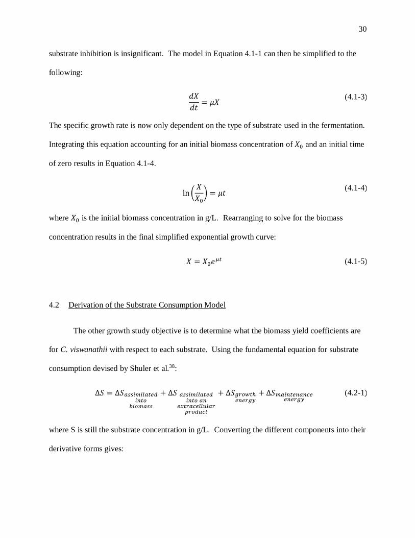
substrate inhibition is insignificant. The model in Equation 4.1-1 can then be simplified to the
following:
𝑑𝑋
𝑑𝑡= 𝜇𝑋
(4.1-3)
The specific growth rate is now only dependent on the type of substrate used in the fermentation.
Integrating this equation accounting for an initial biomass concentration of 𝑋0 and an initial time
of zero results in Equation 4.1-4.
ln (𝑋
𝑋0) = 𝜇𝑡
(4.1-4)
where 𝑋0 is the initial biomass concentration in g/L. Rearranging to solve for the biomass
concentration results in the final simplified exponential growth curve:
𝑋 = 𝑋0𝑒𝜇𝑡 (4.1-5)
4.2 Derivation of the Substrate Consumption Model
The other growth study objective is to determine what the biomass yield coefficients are
for C. viswanathii with respect to each substrate. Using the fundamental equation for substrate
consumption devised by Shuler et al.38:
Δ𝑆 = Δ𝑆𝑎𝑠𝑠𝑖𝑚𝑖𝑙𝑎𝑡𝑒𝑑𝑖𝑛𝑡𝑜
𝑏𝑖𝑜𝑚𝑎𝑠𝑠
+ Δ𝑆 𝑎𝑠𝑠𝑖𝑚𝑖𝑙𝑎𝑡𝑒𝑑𝑖𝑛𝑡𝑜 𝑎𝑛
𝑒𝑥𝑡𝑟𝑎𝑐𝑒𝑙𝑙𝑢𝑙𝑎𝑟𝑝𝑟𝑜𝑑𝑢𝑐𝑡
+ Δ𝑆𝑔𝑟𝑜𝑤𝑡ℎ𝑒𝑛𝑒𝑟𝑔𝑦
+ Δ𝑆𝑚𝑎𝑖𝑛𝑡𝑒𝑛𝑎𝑛𝑐𝑒𝑒𝑛𝑒𝑟𝑔𝑦
(4.2-1)
where S is still the substrate concentration in g/L. Converting the different components into their
derivative forms gives:

31
𝑑𝑆
𝑑𝑡= −
1
𝑌𝑋 𝑆⁄
𝑑𝑋
𝑑𝑡−
1
𝑌𝑃 𝑆⁄
𝑑𝑃
𝑑𝑡− 𝑚𝑋
(4.2-2)
where 𝑌𝑋 𝑆⁄ is the biomass yield coefficient with units of g/L biomass per g/L substrate, 𝑌𝑃 𝑆⁄ is
the product yield coefficient with units of g/L product per g/L substrate, and 𝑚 is a maintenance
coefficient in g/L substrate per g/L biomass ∙ hr. It is assumed that the growth energy term is
lumped into the maintenance energy term. To further simplify this model, it is assumed that the
maintenance term is significantly smaller than the biomass term, since only the exponential
growth regime is of interest and the cells would be focusing on assimilating the substrate into
biomass. Next, the product formation term is assumed to be negligible as well, since the growth
studies do not add any feedstock to form the product of interest. There is a possibility that the
Crabtree effect could be occurring, since the yeast are grown with a large excess of substrate;
however steady-state conditions are typically needed to induce ethanol formation and since this
is a batch process, the amount of ethanol formation should be relatively small after the
concentration of sugars is reduced within the first couple of hours39. Future studies should be
conducted to verify that the ethanol concentration is small comparatively to the substrate
concentration. The substrate consumption rate equation is therefore reduced to one term:
𝑑𝑆
𝑑𝑡= −
1
𝑌𝑋 𝑆⁄
𝑑𝑋
𝑑𝑡
(4.2-3)
Substituting in Equations 4.1-3 and 4.2-4, a simple ordinary differential equation can be formed:
𝑑𝑆
𝑑𝑡= −
μ𝑋0
𝑌𝑋 𝑆⁄𝑒𝜇𝑡
(4.2-4)
Integrating Equation 4.2-4 while accounting for an initial substrate concentration of 𝑆0 and an
initial time of zero gives:

32
𝑆 − 𝑆0 = −𝑋0
𝑌𝑋 𝑆⁄𝑒𝜇𝑡 +
𝑋0
𝑌𝑋 𝑆⁄
(4.2-5)
Rearranging for substrate concentration and simplifying the right-hand side results in the final
form of the substrate consumption curve:
𝑆 = 𝑆0 +𝑋0
𝑌𝑋 𝑆⁄(1 − 𝑒𝜇𝑡)
(4.2-6)
4.3 Further Development of Models for Analysis in RStudio
The parameters of interest in the growth study are the specific growth rates of each
substrate tested and the biomass yield coefficients, which were modeled using RStudio with the
R code presented in Appendix B. The biomass yield coefficients are only applicable with the
media used in this experiment, so in order to replicate the values, OPT1 medium should be used
with the chemicals in Appendix C and the recipe in Appendix A.
In order to derive a regression model for each of the above analytical models, nonlinear
mean modeling will be used with indicator variables that capture the variability between trials.
The models will be derived in a similar manner that is done with mixed effects modeling, which
is built from two parts: an individual-level model and a population-level model. In the individual
model, instead of capturing the biological variability of flasks like in mixed effects modeling, the
model aims to encompass all replicates conducted under the same condition. The parameters at
the individual level may then be expanded on with the population-level model, where the
between-trial variation can be added40.
For the biomass growth curves, the following individual-level regression model is used,
based on Equation 4.1-5:

33
𝑋𝑖𝑗 = 𝛽0,𝑖𝑒𝛽1,𝑖∙𝑡𝑖𝑗 + 𝜖𝑖𝑗 (4.3-1)
where 𝛽 indicates a placeholder parameter that will be expanded on by the population-level
model, 𝜖 represents any measurement error in collecting the data, subscript 𝑖 denotes the culture
flask that was sampled, and subscript 𝑗 indicates a specific data point used for a given sample
time. This individual model is an average over all the time points at which data was collected
within the same trial conditions. In this case, 𝜖𝑖𝑗 is considered negligible compared to the
variance seen between cultures grown at different conditions. The placeholder variables can be
expanded with the population-level model, reflected in Equations 4.3-2 and 4.3-3.
𝛽0,𝑖 = 𝑋0 + 𝛼4 ∙ (𝐺𝑙𝑢𝐺𝑙𝑦) + 𝛼5 ∙ (𝐺𝑙𝑢𝑋𝑦) (4.3-2)
𝛽1,𝑖 = 𝜇1 ∙ (𝐺𝑙𝑢𝑐𝑜𝑠𝑒) + 𝜇2 ∙ (𝐺𝑙𝑦𝑐𝑒𝑟𝑜𝑙) + 𝜇3 ∙ (𝑋𝑦𝑙𝑜𝑠𝑒) + 𝜇4 ∙ (𝐺𝑙𝑢𝐺𝑙𝑦) + 𝜇5
∙ (𝐺𝑙𝑢𝐺𝑙𝑦)
(4.3-3)
𝑋0 represents the initial biomass present in each culture on average, and 𝛼1 and 𝛼5 are terms that
account for the variation of the initial biomass concentration due to using one of the
multicomponent media mixtures. 𝐺𝑙𝑢𝑐𝑜𝑠𝑒, 𝐺𝑙𝑦𝑐𝑒𝑟𝑜𝑙, 𝑋𝑦𝑙𝑜𝑠𝑒, 𝐺𝑙𝑢𝐺𝑙𝑦, and 𝐺𝑙𝑢𝑋𝑦 are indicator
variables that are converted to a 1 when that particular carbon substrate or substrate mix is
included in the media. Indicator variables allow for the same parameter to be solved for many
different subjects, letting them have their own unique values. The numerical subscripts for the
specific growth rate indicate that it is the specific growth rate of C. viswanathii on the carbon
substrate it was grown on, where 1 is glucose, 2 is glycerol, 3 is xylose, 4 is a 2:1 mixture of
glucose and glycerol, and 5 is a 2:1 mixture of glucose and xylose. The reason for creating
separate terms for the multicomponent substrate mixtures will be discussed further when
analyzing the results in 7.1 of the Discussion section.

34
For the substrate consumption curves, the following individual-level regression model
was used based on Equation 4.2-4:
−𝑑𝑆
𝑑𝑡 𝑖𝑗= 𝛽2,𝑖𝑒𝛽3,𝑖∙𝑡𝑖𝑗 + 𝜖𝑖𝑗
(4.3-4)
where the subscripts fit the same description from the previous equations, and the 𝛽 terms are
placeholders for new parameters that are given in the population-level model. Once again, there
are no parameters that capture variability because the specific growth rate is assumed to not vary
with time for a single culture. The biomass yield coefficient is calculated as an average with all
of the data that has been given over time, so no extra terms are given in the individual model to
allow it to vary with time. The measurement error is assumed to be negligible again compared to
the variability observed between trial conditions. Expanding out the placeholder variable gives
the population-level model, illustrated in Equations 4.3-5 and 4.3-6.
𝛽2,𝑖 =𝜇1 ∙ 𝑋0 ∙ (𝐺𝑙𝑢𝑐𝑜𝑠𝑒)
𝑌𝑋/𝑆 1
+𝜇2 ∙ 𝑋0 ∙ (𝐺𝑙𝑦𝑐𝑒𝑟𝑜𝑙)
𝑌𝑋/𝑆 2
+𝜇3 ∙ 𝑋0 ∙ (𝑋𝑦𝑙𝑜𝑠𝑒)
𝑌𝑋/𝑆 3
+𝜇4 ∙ (𝑋0 + 𝛼1) ∙ (𝐺𝑙𝑢𝐺𝑙𝑦)
𝑌𝑋/𝑆 4
+𝜇5 ∙ (𝑋0 + 𝛼2) ∙ (𝐺𝑙𝑢𝑋𝑦)
𝑌𝑋/𝑆 5
(4.3-5)
𝛽3,𝑖 = 𝜇1 ∙ (𝐺𝑙𝑢𝑐𝑜𝑠𝑒) + 𝜇2 ∙ (𝐺𝑙𝑦𝑐𝑒𝑟𝑜𝑙) + 𝜇3 ∙ (𝑋𝑦𝑙𝑜𝑠𝑒) + 𝜇4 ∙ (𝐺𝑙𝑢𝐺𝑙𝑦) + 𝜇5
∙ (𝐺𝑙𝑢𝐺𝑙𝑦)
(4.3-6)
The subscripts on the yield coefficients have the same meaning as those for the specific growth
rates. However, the intercept term is now more complicated than in the biomass growth
regression model due to the biomass yield coefficients and specific growth rates varying between
the utilization of each carbon substrate.

35
After combining the individual-level and population-level models to create two overall
regression models, RStudio can then be used to determine the values of the parameters for all of
the substrates and compare them to see if they are statistically different from one another. The
code can be reviewed in Appendix B, but a brief overview of the successes and challenges will
be highlighted here. Note that some of the functions used in this code may not be preset in the
library of RStudio, but could be found in outside sources. A repository of functions was
uploaded from Dr. Eric Reyes for the Biostatistics course at the Rose-Hulman Institute of
Technology40.
In RStudio, indicator variables can easily be created for the substrate type and the model
can then be typed out with all of the indicator variables and parameters of interest. The difficulty
then comes from determining starting values for these parameters. For this project, all data was
first graphically analyzed on Microsoft Excel to obtain an estimate for all of the parameters for
the starting value vector. The last step consists of setting up a nonlinear least squares function,
which regresses the model that was derived with the starting values that were chosen. This
process was done for the growth and substrate consumption curves separately. In order to
determine whether the parameters significantly deviated from one another based on the substrate
type (p-value < 0.05), a matrix was set up to test each of the hypotheses. A unique function,
ParamTest, could then be used to compute p-values based on the characteristic variance-
covariance matrix of the model.
Using the ParamTest function led to statistically sound results for comparing the specific
growth rates; however, the p-values recorded for the yield coefficients cannot be interpreted due
to a number of reasons. First, using the integrated model for substrate versus time would have
led to an analysis that would have had a more clear interpretation of the results, which would be

36
in the context of the substrate concentrations rather than the derivative of them with respect to
time. However, with the limitations observed in RStudio, at least with the available library of
functions, it was found not to be analytically possible to regress the integrated model due to its
complexity. Referencing Equation 4.2-6, the initial substrate concentration varied across the
subjects due to analytical measurement error and how only glucose was added at a lower
concentration in the mixture trials. This would mean that five indicator variables would have to
be included to allow for the initial substrate concentration to vary. However, if the exponential
term shown in Equation 4.3-5 were integrated, then there would be another intercept term with
its own set of indicator variables. This caused the nonlinear least squares function not to
converge when it attempted to find a solution to the regression model. Another issue occurred
when the specific growth rates in Equations 4.3-5 and 4.3-6 were considered to be equal to the
values in Equation 4.3-3. Theoretically, only the substrate consumption curve data would have
to be regressed to get values for specific growth rates, but this model was already too
complicated due to the number of parameters that were included. For the purposes of extracting
at least approximate estimates for the yield coefficients from the regression model, the specific
growth rates found in the growth curve model were substituted into this substrate consumption
model. This completely omits any ability to make statistical inferences from the results to
accurately compare the yield coefficients between the substrates.
For all of the equations that were derived in this section, it is assumed that the models
were defined correctly from scientific principles. Another assumption is that the errors resulting
from the model fit have a mean of zero and constant variance, and do not conform to any
particular correlation structure. Lastly, it is assumed that the biological variability is much
smaller than the variability seen in the trials conducted at different conditions. This is the

37
greatest limitation observed, which could be overcome by using a more complex mixed effects
model that accounts more for that particular variability. Although this method has less statistical
power than if a nonlinear mixed effects model was used, it is thought to be adequate for the
comparison of growth parameters between the conditions used.

38
5. MATERIALS AND METHODS
5.1 Description of the Major Equipment Used
For the experiments conducted, there are two major pieces of equipment that were
utilized. First is the YSI bioanalyzer, which was used to determine substrate concentrations for
glucose, xylose, and glycerol. This instrument was important for constructing the substrate
consumption curves during the growth studies of C. viswanathii and for checking that the
concentration of substrate was held approximately constant for the production studies. Secondly,
gas chromatography with mass spectrometry (GC-MS) was used to determine the concentration
of various metabolites and products in the production study. Components in the solution are
separated by boiling point and then fragmented with electrons to record a series of mass-to-
charge ratios (m/z) that can be used to identify the components. Another instrument that was
used, but is not considered a focus of this project, is a high-performance liquid chromatography
column (HPLC). HPLC was used in order to analyze the production samples and compare the
results to those obtained from GC-MS in order to see if the method could be verified. It
separates the components on the basis of polarity instead of their boiling points, which
eliminated the need for a derivatization step in that section of the analysis. For a list of all
chemicals used in this experiment, except for those used to operate the bioanalyzer, see
Appendix A. The YSI bioanalyzer specific chemicals are presented in the following section.

39
5.1.1 YSI Bioanalyzer
The instrument used to determine substrate concentration was a YSI 2900 Series
Biochemistry Analyzer. It uses various membranes containing immobilized enzymes to turn
over a specific substrate, which generates a voltage that can be correlated to a concentration in
g/L using internal algorithms. A typical sample takes about a minute on average to process, and
the injected sample size can range from 10 µL to 50 µL. A maximum of six metabolites can be
measured in a single sample, but the instrument was used in this experiment with a maximum of
two enzymatic membranes active at one time, allowing for only two metabolites to be tested for
simultaneously. Some membranes require a unique buffer to be used, as in the case of galactose
oxidase, but the system was set up so that only one buffer could be used at once. Therefore,
glycerol concentration was always sampled independently of glucose and xylose. Glucose and
xylose can be measured simultaneously or separately with the materials and parameters given in
Table 5.1.1.1 since they require the same buffer. The xylose membrane, pyranose oxidase, is
responsive to the presence of glucose in solution, so when cultures were tested that were grown
on xylose stock solution, it was assumed that there was no glucose present in the samples so that
the xylose membrane could be used independently. The materials and parameters for glycerol
measurement can also be reviewed in Table 5.1.1.141.
Note that the YSI 2705 buffer is sensitive to light and must be stored in an opaque bottle.
However, an opaque YSI 2935 bottle was not available, so the general buffer bottle was covered
in aluminum foil along with the tubing when using the glycerol membrane and buffer.

40
Table 5.1.1.1: List of materials and parameters for all membrane configurations to
determine substrate concentration on the YSI 2900 Bioanalyzer41.
Substrate
Tested
Glucose Xylose Glucose +
Xylose
Glycerol
Buffer YSI 2357 YSI 2357 YSI 2357 YSI 2705
Calibration
Standard
YSI 2776
2.50 g/L
YSI 2767
20.0 g/L
YSI 2776 &
YSI 2357
YSI 7141
25.0 g/L
Membrane
YSI 2365
glucose oxidase
YSI 2761
pyranose oxidase
YSI 2365 &
YSI 2761
YSI 7140
galactose oxidase
Detection
Range
0.05 – 18.0 g/L 0.5 – 30.0 g/L similar to xylose 0.75 – 40.0 g/L
Sample Size 10 µL 13 µL 13 µL 10 µL
Precision
2% or 0.02 g/L,
whichever is
greater
2% or 0.5 g/L,
whichever is
greater
2% or 0.1 g/L
whichever is
greater
3% at calibration
point
Linearity ±5% ±10%
±5% or 0.5 g/L,
whichever is
greater
±5% or 0.75 g/L,
whichever is
greater
5.1.2 GC-MS
The column used was an Elite 5MS capillary column, which was 30 m long with a 0.25
mm inner diameter and 0.25 µm film thickness. The stationary phase was made of 1,4-
bis(dimethylsiloxy)phenylene dimethyl polysiloxane, which has low polarity and bleed and is

41
relatively inert so it works well for the separations of derivatized DCAs and FFAs. Helium gas
was used for the mobile phase42. Elite 5MS columns can be operated within temperature
limitations of -60°C and 330-350°C, but it was recommended by the technician not to run the
column over 250°C for extended periods of time43.
The GC-MS system used was a QP2010S manufactured by Shimadzu of Japan. The
maximum oven and injection port temperature that can be reached is 450°C, while the maximum
pressure that can be reached with the advanced flow controller is 970 kPa. The mass
spectrometer system is directly connected to the capillary column. It can be operated with
temperatures between 50°C and 350°C, while the ion source temperature can range from 140°C
to 260°C with an electron energy of 10 to 200 eV. The mass analyzer is a metal quadrupole
mass filter with a pre-rod that can detect m/z values between 1.5 and 1000 with electron impact
ionization. The high-speed scan rate can reach 10000 amu/sec. The resolution is 2 m/z units at
full-width half maximum44. The specific parameters used for these experiments will be
discussed further in Section 5.4.2.
5.1.3 HPLC
The column used for the HPLC system was an Aligent TC-C18 (2), which was 250 mm
long with an internal diameter of 4.6 mm and a particle size of 5 µm. The stationary phase
support is made up of ultra-pure octadecyl silica with a very high surface area and a pore size of
about 170 Å. It can handle a wide pH range and can be well-suited for the use of reversed-phase
liquid chromatography. An Aligent Infinity 1220 II LC system was used equipped with two
different detectors. A refractive index detector (RID) and a diode array detector (DAD) were
used to determine concentration45,46.

42
5.2 Preparation of Cell Bank
A sterile loop was used to remove cells from the surface of a cell stock of ATCC®
20962TM, which was stored at -80°C. This loop was then used to streak a plate containing YPD
media in order to form isolated colonies. Formulation of the YPD media is given in Appendix
A. The plate was then put in an incubator at 30°C for 24 hours. A single colony was then used
to inoculate a Falcon™ tube containing 3 mL of OPT1 medium, for which the recipe is also given
in Appendix A. After another 24 hours of growth at 30°C and 250 rpm, two 250 mL plastic
baffled flasks were inoculated with 300 µL of culture grown in the tube. One was used to check
the optical density of the yeast, to estimate the measurement of growth, without perturbing the
other flask. After 8 hours of growth at 30°C and 250 rpm, the optical density at 600 nm
(OD600) was determined to be 2.02 at a dilution of 50%, which was considered high enough for
cell bank preparation, but low enough that the yeast would still be in the exponential growth
phase. For the cell bank, 30 cryovials were filled with 500 µL of culture from the unperturbed
flask. A 30% glycerol solution was then added to dilute each sample by half. The cryovials
were stored in a -80°C freezer for the remainder of the study, where they were used at the rate of
one vial per week for each set of experiments.
5.3 Growth Study Method and Conditions
The growth of C. viswanathii was studied on five different carbon sources: glucose,
xylose, glycerol, a mixture of glucose and xylose, and a mixture of glucose and glycerol. Each
experiment was run with at least three biological replicates to account for any chance mutations

43
or variability in the culture to adapt to the media. To prepare the biological replicates, a seed
flask would be inoculated the night before with 300 µL of cell bank culture into 30 mL of the
OPT1 media, with all of the components added including the substrate. The volume of the
substrate added was always kept constant at 5 mL, even though the solution of 150 g/L xylose
contained a smaller mass of available carbon than the solutions of 180 g/L glucose and 180 g/L
glycerol. The mixtures of glucose with xylose and glucose with glycerol were always on a 2:1
volume basis, so that 3.3 mL of glucose was always added to 1.7 mL of xylose or glycerol.
After growing the seed culture for approximately 18 hours at 30° C and 250 rpm in a 250
µL plastic baffled flask, three flasks would be given a 1% inoculum, where 300 µL of the seed
culture would be added to 30 mL of the same media composition. In the case of a mixture of
glucose with xylose or glycerol, the seed culture would just contain glucose so that an additional
set of three glucose flasks could be inoculated and studied for comparison. An original optical
density at 600 nm (OD600) was determined by measuring the apparent absorbance of the seed
culture and then accounting for the inoculum dilution.
Optical density is the measurement of the reduction of light intensity, accounting for the
refraction or scattering of light47. It is often approximated by an absorbance value recorded at
600 nm, which must be below the value of 1 to get an accurate approximation for concentration.
This requires a serial dilution of the samples to be within the appropriate range. The dilution
factor was gradually increased as samples were taken over time, starting at 1/4 for after two or
three hours of growth, and ending at 1/200 for after 18 or more hours of growth. Cuvettes with a
path length of 1 mm were used to contain the samples while they were placed in a Thermo
Scientific NanoDrop OneC spectrophotometer for OD600 measurements. This type of UV-Vis
spectrophotometer has a relatively high accuracy of ±3% and a repeatability of 0.002 absorbance
44
units, so absorbance measurements were only taken once for each sample48. A linear calibration
curve could be created to correlate the adjusted absorbance value after serial dilutions to a
concentration of dry cell weight per liter of medium. Dry cell weights were determined by
drying 1.7 mL microcentrifuge tubes for 48 hours, then adding random samples of culture over
time to them with a known OD600, then removing the supernatant with the process described
below and further drying the pellet for another 48 hours at 80°C.
The growth study flasks were then grown for the next 10 to 12 hours at 30° C and 250
rpm, with samples for OD600 measurements taken every 1-2 hours. A final OD600 was
measured the next day after 24 hours of growth. With every OD600 measurement, 1 mL aliquots
were additionally taken from each flask to determine the substrate concentration. These aliquots
were put in 1.7 mL microcentrifuge tubes and then put in a centrifuge for 5 minutes at 15,000xg
and room temperature. The supernatant was collected using an Eppendorf pipette and transferred
to another tube for storage. The tubes were frozen at -20°C until all samples were collected, so
that a given trial could be tested all at once.
5.3.1 YSI Bioanalyzer Setup and Calibration
Once the samples were all prepared, they were thawed out and shaken by hand to ensure
they were homogenous. After various attempts at troubleshooting, it was found that aiming for
concentrations below 10 g/L for glucose and xylose would produce the most accurate results.
Since the starting concentration was 30 g/L for glucose, it was determined that diluting the
samples 4-fold was conservative enough to bring the concentration down to the desired level.
Xylose samples were also diluted to the same degree, even though the starting concentration of
25 g/L was lower than the upper value of the detectable range. Glycerol had a high range of

45
detectability, so the samples were not diluted for the analysis. However, in the case of a mixture
of glucose and glycerol, half of each sample was taken and diluted 4-fold for the glucose
measurement, while the other half was left undiluted. If a mixture of glucose and xylose was
used, the entire sample was diluted 4-fold and tested with the simultaneous glucose and xylose
measurement.
Before processing the prepared samples, the membrane viability was checked. If a
membrane was more than a month old, it was switched out for a new one. On average, the
membranes have a life of about 1-2 weeks if the machine is regularly calibrated. It was
determined that the membranes could still be used after this if standards were tested at regular
intervals. The membrane would gradually deteriorate with time, but the standards would help to
make a calibration curve to determine the activity loss. For each combination of substrates
tested, 3-5 standards were produced with concentrations that covered the range of expected
values from the samples. The standards were loaded first, followed by 8-12 samples. Although
the sampling tray could hold up to 24 samples, fewer samples were tested at a time since the
machine recalibrated itself after analyzing 10 samples. This allowed for the standards to be
measured again after each calibration to adjust for the loss of membrane activity.
5.4 Production Study Method and Conditions
The production of LCDCAs was studied by varying the carbon source, the concentration
of the carbon source, and the feedstock provided to the yeast. A list of the experimental
conditions varied is given in Table 5.4.1. Oleic acid, C18:1, was chosen to be representative of
DCO because a large percentage of the oil is comprised of unsaturated C18 fatty acids. Methyl
oleate was used because it is the ester form of oleic acid and is a liquid at the room temperature

46
and other temperatures typically used for yeast fermentations. The same carbon sources were
used from the growth experiments, except the mixtures were omitted. A higher bound and a
lower bound concentration were tested in order to show whether substrate inhibition was
occurring during LCDCA production. The feedstock concentration was kept constant at 10 g/L.
Note that the technical grade methyl oleate that was used contained about 71-90% C18 esters,
and only about 65% of that was methyl oleate. An average purity of 52.3% was assumed, and
the amount of the technical grade stock added was based on a total amount of 10 g/L of the
methyl oleate component being added. The same concept applies to the oleic acid used, which
has a purity of 90%. A complete list of chemicals used and their manufacturers can be reviewed
in Appendix C.
Each trial conducted lasted a week and tested two sets of conditions in which only the
carbon source concentration differed. This was done partly to increase the number of flasks
managed at once. By only varying the substrate concentration, there was also no need to worry
about accounting for an extended lag phase in the growth since the type of carbon source was
unchanged from the seed culture. The seed cultures were prepared similarly to those made in the
growth studies, except they were grown at 30°C and 250 rpm for 24 hours. A single seed culture
would be used to inoculate seven 250 mL plastic baffled flasks the next day with 300 µL
transferred to 30 mL of medium, another 1% inoculum. These seven flasks consisted of three
biological replicates for a carbon source concentration of 10 g/L and three more for a
concentration of 25 g/L. The remaining flask was considered a control that would be analyzed to
ensure that no product was being formed.

47
Table 5.4.1: List of experimental conditions for all trials conducted in the production of
LCDCAs with C. viswanathii.
Carbon Source Carbon Source Concentration Feedstock
Glucose 10 g/L Methyl Oleate
Glucose 25 g/L Methyl Oleate
Xylose 10 g/L Methyl Oleate
Xylose 25 g/L Methyl Oleate
Glycerol 10 g/L Methyl Oleate
Glycerol 25 g/L Methyl Oleate
Glucose 10 g/L Oleic Acid
Glucose 25 g/L Oleic Acid
Xylose 10 g/L Oleic Acid
Xylose 25 g/L Oleic Acid
Glycerol 10 g/L Oleic Acid
Glycerol 25 g/L Oleic Acid
After shaking for another 24 hours at 30°C and 250 rpm, the cells in the production flasks
had reached the desired stationary phase. The biomass concentration was assumed to have
reached a maximum, and the biotransformation was then induced. First, 250 µL aliquots were
obtained from each flask to serve as a check that the carbon substrate had been completely
consumed. They were collected and the pellets were spun down and removed according to the
process described in Section 5.3. Then the appropriate amount of carbon substrate was added to
each of the flasks to reach the desired concentration, with the control flask being held at an
arbitrary concentration of 10 g/L. Methyl oleate or oleic acid was then added to give six

48
experimental flasks an initial concentration of 10 g/L, based off of the original media volume of
30 mL, which correlates to 0.3 g of material added. All components were considered in terms of
concentration and not mass due to how the calibration curves generated for the gas
chromatography analysis relate peak area to concentration, see Section 6.1. The control flask
was not given any feedstock in each trial.
Once the feedstock had been added, initial production samples were taken to give a more
accurate estimate of how much feed was in the medium and what impurities are present. The
production samples were 400 µL aliquots, which were then separated from the biomass pellet as
described earlier. Sometimes solubility issues of fatty acids and DCAs occurred where solids or
oil floated on top of the supernatant, so those immiscible components were carefully pipetted
with the supernatant to the new microcentrifuge tube. Formation of these solids and oil phases
could sometimes be mitigated with the adjustment of culture pH. The pH of each flask was
adjusted twice a day with 1 N sodium hydroxide, once before samples are taken and then around
7-8 hours later. Enough base was added so that the pH was about 7.5-8 but no more than 9. A
higher pH resulted in cell lysis, while a lower pH could reduce the solubility of feed and
products, which was known to affect the rate of the biotransformation. Lastly, an OD600
measurement was taken for each of the flasks to see if product precipitate had begun forming.
Each sample required a 1:200 dilution to be within the appropriate range discussed to test for the
optical density.
After 24 and 48 hours of biotransformation, the pH would be adjusted for the first time
each day using 1 N sodium hydroxide to about 7.5-8. Then another set of 250 µL and 400 µL of
samples would be taken from each flask, including the control. Once the sample tubes were
stored in the freezer at -20°C, the same volume of carbon substrate as last time would be added

49
to each flask to maintain a close to constant concentration. Optical density would once again be
checked by using an OD600 measurement. Finally, the pH would be adjusted later after 7-8
hours to help with solubility issues. Cell viability was optionally checked after 24 hours by
taking a 10 µL sample from each flask and diluting it into 990 µL of water. A serial dilution
would be done so that samples would be plated on YPD medium with a 1:100 dilution, 1:10,000
dilution, and a 1:1,000,000 dilution. The water and microcentrifuge tubes used in this case were
sterilized to prevent any contamination. The plates would be grown for 24-48 hours or until
small, defined colonies appeared. This method was used at any time where flask contamination
was a concern based on a significant change in OD600 or biomass pellet size and appearance
when collecting samples. As a reference below, C. viswanathii is shown to have circular, light
cream colored colonies that are mainly smooth and glistening.
Figure 5.4.1: C. viswanathii is plated on YPD agar to determine cell viability in the first
production study conducted. The dilutions of the samples from left to right are 1:100,
1:10,000, and 1:1,000,000. A simple circular and smooth morphology is observed.
After 72 hours of biotransformation, the process of adjusting pH, collecting samples, and
checking optical density was done again, but this time the addition of carbon substrate was
omitted. LCDCA production is assumed to be occurring at a much slower rate at this point since

50
the fermentation is occurring in a batch fashion where the feedstock and other micronutrients
have not been replenished. The cultures were allowed to grow without the addition of substrate
or sodium hydroxide for the next 48 hours, simulating LCDCA production with nutrient and
substrate depletion for the batch fermentation cycle. Final 250 µL and 400 µL samples were
taken after a total of 120 hours of biotransformation. The pH was adjusted immediately
beforehand if needed, and the optical density was checked again immediately afterward. Each
culture was plated to determine if cells were still living after the long period of environmental
stress with metabolite buildup. After the flasks were cleaned that day, another starter culture
would be prepared with new conditions since each study lasted an entire week.
5.4.1 Original Extraction and Derivatization Method of Production Samples
LCDCAs, fatty acids, and methyl esters first need to be extracted from the aqueous
fermentation broth to an organic solvent prior to analysis. It is known that acidifying the broth
causes the LCDCAs to precipitate, which favors the partitioning of the acids into the organic
phase so that they can dissolve31. Therefore, the 400 µL production study samples were mixed
with 160 µL 1 N HCl and 800 µL methyl tert butyl ether (MTBE) in the microcentrifuge tubes.
In order to make ensure that phase and chemical equilibrium were obtained, the tubes are shaken
for 3 hours at a setting of 2.5 out of 10 on a VWR Standard Heavy-Duty Vortex Mixer. It is
estimated that the analog setting of 5 corresponds to 900 rpm, so the setting used in this study is
assumed to be close to 450 rpm based on that heuristic49.
Prior to derivatizing the components in the organic phase, the tubes were first removed
from the shaker and placed in a centrifuge at 15,000xg for a minute in order to expel any water
that was entrained in the organic phase. GC autosampler vials were then labeled and 125 µL of

51
the organic phase were transferred from the respective microcentrifuge tube. To each extracted
sample, 12.5 µL pyridine and 50 µL N-methyl-N-(trimethylsilyl)trifluoroacetamide (MSTFA)
were added to derivatize them. Derivatization, in this case, is the reaction of the carboxyl groups
of the LCDCAs and FFAs into silyl groups in order to reduce the boiling point of the compounds
by a significant degree. For example, literature sources state that the boiling points of oleic acid
and similar length FFAs are around 162-383°C at atmospheric pressure, which could exceed the
limit of the column used in this study50. The creation of trimethylsilyl (TMS) derivatives allows
for all of the components of interest to boil under 280°C.
Derivatization with MSTFA requires some heating of the samples and mixing in order for
the reaction to go to completion. Based on the reported protocol from Rimmel, the samples for
this experiment were either vortexed or shaken vigorously for 10 seconds31. This study then
derivatized the LCDCAs and other components at 60°C for 20 minutes, which was determined to
be a short enough time to produce calibration curves while preventing the breakdown of long-
chain components, as discussed in Section 7.2. Once the derivatization reaction was complete,
462.5 µL MTBE was added to each sample to dilute the concentration and bring the liquid level
in the vials to the half-way mark so that the GC syringe could reach the sample. Then 25 µL of a
2.6 g/L stock of methyl pentadecanoate (PME, C15:0) and 2.6 g/L stock of methyl
heptadecanoate (HME, C17:0) were added as internal standards (IS).
5.4.2 Gas Chromatography and Mass Spectrometry Parameters
A summary of all of the GC-MS parameters is given in Tables 5.4.2.1 and 5.4.2.2. The
temperature ramp devised was set up to be slower than the ramps used by Rimmel and Funk et
al. to make sure the peaks had good resolution for all of the media components1,31. A rapid

52
increase in temperature at the end was implemented in order to help remove any LCDCAs that
may have been stuck on the column. The column flow, total flow, purge flow, and split ratio for
the column were selected based off of other methods used on the instrument that were devised by
the lab technician. Injection temperatures of 275°C and 300°C were used on each sample,
although Restek recommends not going above 200°C in order to avoid breakdown of TMS
derivatives51. It was found that the lower temperature was not high enough to volatize the
majority of the chemicals analyzed in Section 7.3.
All samples were injected with an autosampler that used a medium speed for the suction
and injection of the liquid, along with five solvent rinses before and after contacting the sample
and a single sample rinse before injecting the sample. An injection size of 2 µL was used, which
was determined to be close to the maximum injection volume to prevent excessive back flash, as
shown by the solvent expansion calculator in Figure 6.2.8 in Section 6.2 programmed by
Restek52. Since the gradient ramp for temperature took 34 minutes per sample, and the amount of
time it took the column to cool from 280°C to 160°C with ambient convection was about 15 to
20 minutes, it took almost an hour to process each sample. The autosampler used had 12 slots
available, so throughout the experiment, the samples were analyzed by GC-MS overnight so that
the instrument would be available the next morning for others to use.
A list of the retention times for all of the chemicals tested can be reviewed in Appendix D
and the final calibration curves used for octadecanedioic acid (C18:0 DCA), methyl oleate (MO),
oleic acid (OA), and stearic acid (SA) can be found in Section 6.2. A summary of the
differences in the initial method used in this study, devised from the original work of Rimmel’s
dissertation, can be seen in Table 7.2.1.

53
Table 5.4.2.1: Summary of the parameters set for the gas chromatography column, after
the modifications made in this study.
Parameter Set Value
Column Oven Temperature 160°C
Injection Temperature 275°C or 300°C
Injection Mode Split
Flow Control Mode Linear Velocity
Pressure 12.3 psi
Total Flow 9.0 mL/min
Column Flow 0.89 mL/min
Linear Velocity 36.0 cm/s
Purge Flow 1.0 mL/min
Split Ratio 8.0
Temperature Ramp
Hold at 160°C for 5 min
Increase by 5°C/min until 280°C
Hold at 280°C for 5 min
Increase by 20°C/min until 300°C
Hold at 300°C for 1 min
Total Program Time: 36 min
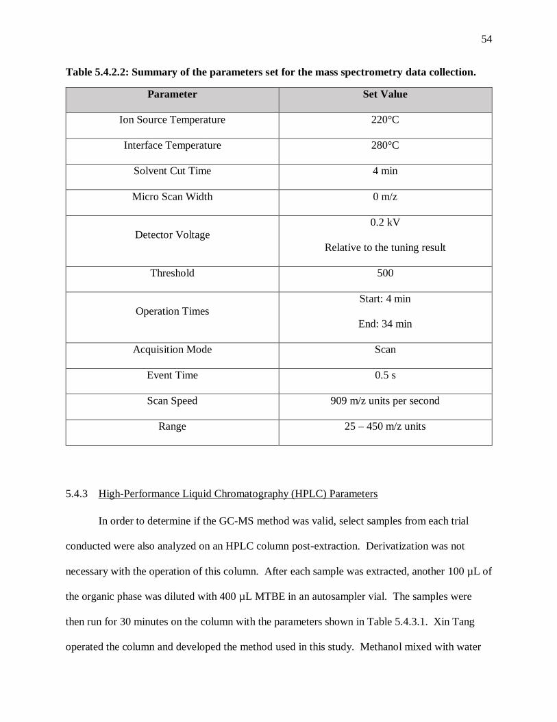
54
Table 5.4.2.2: Summary of the parameters set for the mass spectrometry data collection.
Parameter Set Value
Ion Source Temperature 220°C
Interface Temperature 280°C
Solvent Cut Time 4 min
Micro Scan Width 0 m/z
Detector Voltage
0.2 kV
Relative to the tuning result
Threshold 500
Operation Times
Start: 4 min
End: 34 min
Acquisition Mode Scan
Event Time 0.5 s
Scan Speed 909 m/z units per second
Range 25 – 450 m/z units
5.4.3 High-Performance Liquid Chromatography (HPLC) Parameters
In order to determine if the GC-MS method was valid, select samples from each trial
conducted were also analyzed on an HPLC column post-extraction. Derivatization was not
necessary with the operation of this column. After each sample was extracted, another 100 µL of
the organic phase was diluted with 400 µL MTBE in an autosampler vial. The samples were
then run for 30 minutes on the column with the parameters shown in Table 5.4.3.1. Xin Tang
operated the column and developed the method used in this study. Methanol mixed with water

55
and acetic acid was found to be compatible with the MTBE solvent used and chosen to be the
isocratic mobile phase used throughout the analysis. Data was collected from both the DAD and
RID detectors for the comparison, much like how two internal standards were used in the GC-
MS method to account for new sources of variability. Calibration curves were made with the
same standards used for the GC-MS, and the unsaturated C18:1 DCA peak was determined by
comparing the resulting chromatographs of samples to GC chromatographs of the same samples
reporting that the C18:1 DCA was present.
Table 5.4.3.1: Summary of the HPLC parameters used for the secondary analysis of the
extracted production study samples.
Parameter Set Value
Mobile Phase
90 % (v/v) Methanol
9.9 % (v/v) Water
0.1% (v/v) Acetic Acid
Flow Rate 1.0 mL/min
Injection Volume 5 µL
Column Oven Temperature 35°C
RID Temperature 32°C
Column Pressure 94 bar
DAD UV Wavelengths
210 nm
250 nm
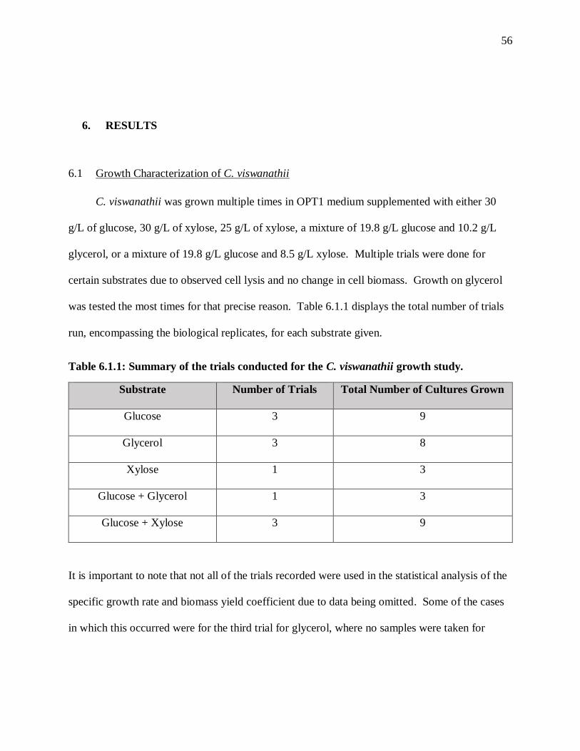
56
6. RESULTS
6.1 Growth Characterization of C. viswanathii
C. viswanathii was grown multiple times in OPT1 medium supplemented with either 30
g/L of glucose, 30 g/L of xylose, 25 g/L of xylose, a mixture of 19.8 g/L glucose and 10.2 g/L
glycerol, or a mixture of 19.8 g/L glucose and 8.5 g/L xylose. Multiple trials were done for
certain substrates due to observed cell lysis and no change in cell biomass. Growth on glycerol
was tested the most times for that precise reason. Table 6.1.1 displays the total number of trials
run, encompassing the biological replicates, for each substrate given.
Table 6.1.1: Summary of the trials conducted for the C. viswanathii growth study.
Substrate Number of Trials Total Number of Cultures Grown
Glucose 3 9
Glycerol 3 8
Xylose 1 3
Glucose + Glycerol 1 3
Glucose + Xylose 3 9
It is important to note that not all of the trials recorded were used in the statistical analysis of the
specific growth rate and biomass yield coefficient due to data being omitted. Some of the cases
in which this occurred were for the third trial for glycerol, where no samples were taken for

57
substrate concentration, and for the flasks in which the cells had died before the end of the 24
hour growth period.
6.1.1 Specific Growth Rate
Figure 6.1.1.1 shows the resulting data from the study with regards to biomass
concentration, measured from dry cell weight (DCW), versus time. The data was plotted in
RStudio, where it was also analyzed with the code in Appendix B. Most of the data points show
an exponential trend in growth, which can be fit to Equation 4.3-1 well. From an observational
standpoint, the specific growth rates for glucose, glucose and glycerol, and glucose and xylose
should be much higher than those for glycerol and xylose. Characteristic samples of a typical
culture grown on glucose, xylose, and glycerol can be compared in Figure 6.1.1.2. For reference,
a calibration curve for the optical density and biomass concentration can be reviewed in
Appendix E.
Figure 6.1.1.1: Raw data of C. viswanathii grown on various carbon substrates.

58
Figure 6.1.1.2: Comparison of typical growth rates of C. viswanathii on the three separate
carbon sources. Glucose appears to have the highest specific growth rate in the exponential
term, followed by xylose and then glycerol.
When the data was fixed to the previously described mixed effects model, the model
appeared to be a good estimate over time for all combinations of substrate tested, as shown in
Figure 6.1.1.3. There is some slight deviation in the data from the model for glycerol and
glucose mixed with glycerol, where there is a noticeable departure from the average around 7
hours of growth and 9 hours of growth respectively. Table 6.1.1.1 provides a summary of the
specific growth rates found for each substrate and also presents p-values for the hypothesis
testing conducted to see whether the specific growth rates are significantly different from the
value found for glucose. Glycerol, xylose, and the mixture of glucose and xylose had specific
growth rates that were all found to be significantly different on average from that of glucose with
a p-value < 0.05.
y = 0.0486e0.5046x
y = 0.063e0.4358x
y = 0.0703e0.3863x
0
1
2
3
4
5
6
0 1 2 3 4 5 6 7 8 9 10 11 12
Bio
ma
ss,
g/L
Time Elapsed, hr
Glucose
Xylose
Glycerol

59
Figure 6.1.1.3 : Growth study data overlaid with the nonlinear mixed effects model derived
and fit in RStudio. The specific growth rate on glycerol appears to be much smaller than
the other substrates. The mixtures containing glucose and the pure glucose substrate have
the highest values, however, the curves are not overlaid as they would be if they had
identical specific growth rates.
Table 6.1.1.1: Summary of the specific growth rates found for each substrate combination
and the hypothesis testing conducted to determine if the specific growth rates differed
significantly from glucose.
Substrate(s) Specific Growth Rate (𝒉𝒓−𝟏) P-Value
Glucose 0.482 N/A
Glycerol 0.417 0.000
Xylose 0.460 0.003
Glucose + Glycerol 0.405 0.084
Glucose + Xylose 0.386 0.015

60
6.1.2 Biomass Yield Coefficient
Figure 6.1.2.1 illustrates the raw data for the change in consumption rate of carbon
substrates with respect to time, which was modeled for ease of analysis in RStudio as opposed to
the change of substrate concentration with time. Note that the substrate plotted for the mixture
trials is glucose, as the other components were found not to change with time. As the biomass
concentration increases with time, it is expected that the rate of substrate consumption also
increases to accommodate the needs of the multiplying cells. The consumption rate should
follow an exponential trend according to Equation 4.3-4, and that trend is clearly observable for
growth on glucose and glucose mixed with glycerol. Data for growth on xylose, glycerol, and
glucose mixed with xylose appear more scattered and linear. A closer look at the change in
substrate concentration is shown in Figure 6.1.2.2 for a typical culture grown on each substrate.
Significant scatter occurred mostly likely due to the constant recalibration of the YSI
bioanalyzer. Although the change in substrate concentration with time is negative, the
consumption rate should always be positive, but the following graphic shows a few outliers that
have negative values. Once again, negative values should be nonexistent and this error could be
attributed to the membrane degradation and the constant recalibration of the YSI bioanalyzer
needed to help adjust for the membrane uncertainty and hysteresis effects. The xylose
membrane in particular had a consistently high uncertainty of about ± 5% of the total
concentration. However, many of the negative substrate consumption rates appear to be for the
glucose substrate. These data points are from one of the first trials conducted where the
systematic recalibration of the YSI bioanalyzer and the serial dilution methods had not been
developed yet, which could have contributed more error to the analysis compared to the other
trials tested.

61
Figure 6.1.2.1: Raw data of the substrate consumption of C. viswanathii on various
substrates.
Figure 6.1.2.2: Characteristic substrate consumption curves for each type of carbon
substrate.
15
17
19
21
23
25
27
29
31
33
35
0 1 2 3 4 5 6 7 8 9 10 11 12
Su
bstr
ate
Con
ce
ntr
atio
n, g
/L
Time Elapsed, hr
Glucose
Xylose
Glycerol

62
The mixed effects model discussed in Section 4.3 was used to fit the data in RStudio, and
the resulting model was plotted on top of the data in Figure 6.1.2.3. Cultures grown on glucose
and a mixture of glucose and glycerol have a confirmed exponential substrate consumption rate,
while the other substrates do not appear to conform to the model. Hypothesis testing was not
conducted on this part of the study due to the removal of innate variance in the model, as
discussed in Sections 4.3 and 7.1. However, an alternate method to calculating the yield
coefficient was done by subtracting the values of the sixth data point, around 8 hours of growth,
and first data point, around 2 hours of growth, in order to provide another estimate for
comparison to the statistical model. The results are summarized in Table 6.1.2.1, where it is
clearly shown that the biomass yield coefficients are considerably different between the methods
for xylose and glucose mixed with xylose trials.
Figure 6.1.2.3: Substrate consumption rate data overlaid with the nonlinear mixed effects
model derived and fit in RStudio. It appears that growth on glucose mixed with glycerol
has the highest biomass yield coefficient and glycerol has the lowest by a large degree.

63
Table 6.1.2.1: Summary of the values for the biomass yield coefficient on each substrate
determined by both statistical modeling and numerical calculations.
Substrate(s)
Biomass Yield Coefficient
(𝒈 𝑫𝑪𝑾 / 𝒈 𝒔𝒖𝒃𝒔𝒕𝒓𝒂𝒕𝒆)
from statistical model
Biomass Yield Coefficient
(𝒈 𝑫𝑪𝑾/𝒈 𝒔𝒖𝒃𝒔𝒕𝒓𝒂𝒕𝒆)
from numerical analysis
Glucose 0.754 0.566
Glycerol 1.420 1.255
Xylose 1.600 1.105
Glucose + Glycerol 0.547 0.578
Glucose + Xylose 1.230 0.798
From the above table, it would appear that the biomass yield coefficient is high for
xylose, and comparable to that of glycerol. However, when the final biomass and substrate
concentrations are used for the analysis instead, Table 6.1.2.2 illustrates that the xylose trial
resulted in a much lower biomass yield coefficient that was more similar to glucose than
glycerol. The biomass yield coefficients that were reported for the mixture trials are similar to
what resulted from using glucose and xylose. Each trial that was run is reported in the table, and
the trials that did not have data collected for the substrate consumption curves do not have
biomass yield coefficients included. The trial number represents the date at which the substrate
was studied, and if two different substrates were studied, then their data collection began with
the same starter culture.

64
Table 6.1.2.2: Summary of the biomass yield coefficients calculated using the final values
for biomass concentration and substrate concentration, with average final biomass
concentration given for comparison between each trial. Glycerol is shown again to have a
considerably higher biomass yield coefficient than the other substrates on average.
Substrate(s)
Trial
Number
Average Final Biomass
Concentration
(g DCW / L)
Biomass Yield Coefficient
(𝒈 𝑫𝑪𝑾/𝒈 𝒔𝒖𝒃𝒔𝒕𝒓𝒂𝒕𝒆)
With Data from 24 Hours
Glucose 1 43.0 0.323
Glucose 6 36.0 _
Glucose 7 29.3 0.206
Glycerol 2 89.0 1.035
Glycerol 3 70.0 1.100
Glycerol 4 70.0 _
Xylose 3 61.3 0.563
Glucose + Glycerol 5 44.7 0.528
Glucose + Xylose 5 52.7 _
Glucose + Xylose 6 51.3 _
Glucose + Xylose 7 29.3 0.340
6.2 Analytical Method Development
In this section, the individual changes made to the original analytical method will be
illustrated in a chronological fashion. However, the discussion in Section 7.2 will be presented in
a step-oriented organization so that the changes are grouped by whether they occurred for the
extraction, derivatization, or GC-MS analysis steps. Figure 6.2.1 illustrates the experiment in
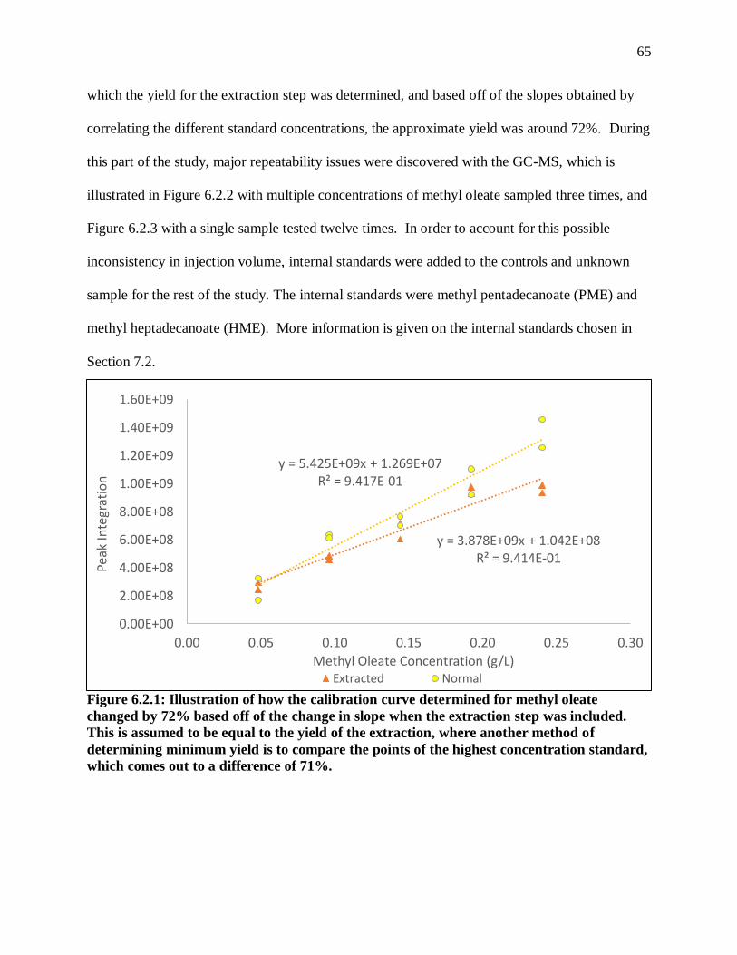
65
which the yield for the extraction step was determined, and based off of the slopes obtained by
correlating the different standard concentrations, the approximate yield was around 72%. During
this part of the study, major repeatability issues were discovered with the GC-MS, which is
illustrated in Figure 6.2.2 with multiple concentrations of methyl oleate sampled three times, and
Figure 6.2.3 with a single sample tested twelve times. In order to account for this possible
inconsistency in injection volume, internal standards were added to the controls and unknown
sample for the rest of the study. The internal standards were methyl pentadecanoate (PME) and
methyl heptadecanoate (HME). More information is given on the internal standards chosen in
Section 7.2.
Figure 6.2.1: Illustration of how the calibration curve determined for methyl oleate
changed by 72% based off of the change in slope when the extraction step was included.
This is assumed to be equal to the yield of the extraction, where another method of
determining minimum yield is to compare the points of the highest concentration standard,
which comes out to a difference of 71%.
y = 3.878E+09x + 1.042E+08R² = 9.414E-01
y = 5.425E+09x + 1.269E+07R² = 9.417E-01
0.00E+00
2.00E+08
4.00E+08
6.00E+08
8.00E+08
1.00E+09
1.20E+09
1.40E+09
1.60E+09
0.00 0.05 0.10 0.15 0.20 0.25 0.30
Peak
Inte
grat
ion
Methyl Oleate Concentration (g/L)Extracted Normal

66
Figure 6.2.2: Repeatability issues are illustrated with the injection volume by how methyl
oleate standards at four different concentrations either exhibited a high or low value for
the peak integration when tested three times each. The actual injection volumes are
unknown, but the parameter was kept constant at 5 µL.
Figure 6.2.3: The inconsistency in the injection volume is clearly illustrated where a single
sample was tested four times, and for each component there was an upper and lower
bound. Minimal scatter is observed. MO is methyl oleate, LAME, is linoleic acid methyl
ester, SAME is stearic acid methyl ester, and the MO isomer is an unidentified compound
that forms a doublet peak with MO in the technical grade solution.
0.0E+00
1.0E+08
2.0E+08
3.0E+08
4.0E+08
5.0E+08
6.0E+08
7.0E+08
8.0E+08
9.0E+08
1.0E+09
0.0 0.1 0.2 0.3 0.4 0.5 0.6
Peak
Inte
grat
ion
Methyl Oleate Concentration (g/L)
Lower Injection Volumes Higher Injection Volumes
0.0E+00
1.0E+07
2.0E+07
3.0E+07
4.0E+07
5.0E+07
6.0E+07
7.0E+07
8.0E+07
9.0E+07
1.0E+08
0.0E+001.0E+082.0E+083.0E+084.0E+085.0E+086.0E+087.0E+088.0E+089.0E+081.0E+091.1E+091.2E+091.3E+09
Peak
Inte
grat
ion
fo
r SA
ME
and
Iso
mer
Peak
Inte
grat
ion
for
MO
an
d L
AM
E
Component
MO LAME SAME MO Isomer

67
Once the internal standards were found to work rather well in accounting for the shift in
peak areas in the chromatographs, the concentrations of MSTFA and pyridine added were
improved with the experiments shown in Figures 6.2.4, 6.2.5, and 6.2.6. It was found that
doubling the amount of MSFTA added improved the calibration curves obtained for oleic acid
and C18:0 DCA. Adding pyridine for a MSTFA to pyridine ratio of either 4:1 or 6:1 did not
seem to significantly affect the calibration curve, so the 4:1 ratio was chosen for the duration of
the production trial analysis. Then, the derivatization time was varied to see if a shorter time
could be used to help prevent the breakdown of fatty acid methyl esters. Figure 6.2.7 shows that
the derivatization time could be reduced to 20 minutes and produced better results than the
control samples derivatized for 40 and 60 minutes. Lastly, Figure 6.2.8 shows the results of
using the Restek solvent expansion calculator to determine the maximum injection volume size.
The injection volume was later changed from 5 µL to 2 µL to prevent excessive back flash as
recommended by this online tool.
Figure 6.2.4: By doubling the amount of MSTFA added, which was already in excess, the
calibration curve for oleic acid improved significantly and there was less scatter in the
data. This improvement was observed for both internal standards used in the study.
0.0
0.5
1.0
1.5
2.0
2.5
3.0
3.5
4.0
4.5
0 0.1 0.2 0.3 0.4 0.5 0.6 0.7
Are
a OA
/ A
rea I
S
Oleic Acid Concentration (g/L)
PME, 50 µLMSTFA
HME, 50 µLMSTFA
PME, 100µL MSTFA
HME, 100µL MSTFA

68
Figure 6.2.5: By doubling the amount of MSTFA added, which was already in excess, the
calibration curve for C18 DCA improved so that there was more of a substantial slope in
the calibration curve. This improvement was observed for both internal standards used in
the study. The data points for the highest concentration of C18 DCA for the 50µL trials
are not included since no peaks appeared in the resulting chromatographs.
Figure 6.2.6: By increasing the ratio of MSTFA to pyridine from 4:1 (12.5 µL of pyridine)
to 6:1 (8.33 µL of pyridine), there appeared to be no significant difference besides a slight
increase in slope, representing a slightly heightened sensitivity.
0.0
0.2
0.4
0.6
0.8
1.0
1.2
1.4
1.6
0 0.1 0.2 0.3 0.4 0.5 0.6 0.7
Are
a DC
A/
Are
a IS
C18:0 DCA Concentration (g/L)
PME, 50 µLMSTFA
HME, 50 µLMSTFA
PME, 100 µLMSTFA
HME, 100µL MSTFA
0
0.5
1
1.5
2
2.5
3
0 0.1 0.2 0.3 0.4 0.5 0.6
Are
a DC
A/
Are
a IS
C18:0 DCA Concentration (g/L)
PME, 12.5µL pyridine
HME, 12.5µL pyridine
PME, 8.33µL pyridine
HME, 8.33µL pyridine

69
Figure 6.2.7: Decreasing the derivatization time at 60°C improves the sensitivity of the
calibration curve significantly, while longer time periods appear to break down the
components since only one concentration was detectable for the 40 minute and 60 minute
samples.
0.0
0.5
1.0
1.5
2.0
2.5
3.0
0.0 0.1 0.2 0.3 0.4 0.5 0.6 0.7
Are
a DC
A/
Are
a IS
C18:0 DCA Concentration (g/L)
20 mins, PME
20 mins, HME
40 mins, PME
40 mins, HME
60 mins, PME
60 min, HME

70
Figure 6.2.8: Calculations done on the solvent expansion calculator by Restek to show that
the maximum injection volume to prevent excessive back flash is 2.2 µL as shown in (B),
but the 5 µL injection volume used previously produces a vapor cloud double the size of the
volume of the liner as shown in (A)52.
(A)
(B)

71
Some of the key chromatographs that summarized how the process improved with time
are shown in the subsequent figures. Figure 6.2.9 shows how a sample with the original
injection temperature of 275°C does not show up in the chromatograph, but when the
temperature is increased to 300°C, a noticeable improvement occurs, but not all of the time as
illustrated in Figure 6.2.10. The chromatograph in Figure 6.2.11 shows a really good example of
what a sample tested looks like when it has a very clear baseline and high resolution at the new
temperature. When the injection temperature gets too high, sometimes random artifact peaks
appear like in Figure 6.2.12, most likely from the degradation of TMS derivatives. There are also
artifact peaks that show up more often than others like the one observed in Figure 6.2.13. Due to
its long retention time, it is possible that it is a degradation product of the derivatized C18:0 and
C18:1 DCAs. Often when oleic acid is derivatized, even in standardized samples, a small peak
will occur around 26.4 minutes as shown in Figure 6.2.14, where the C18:0 DCA peak occurs.
This could be an artifact, but it could also just be DCA that is stuck on the column.
Figure 6.2.9: GC-MS chromatograph representing a production trial sample that is
expected to have oleic acid (OA) in it. The internal standards at 11.3 min (PME) and 15.4
min (HME) are barely present, indicating that either the injection volume or injection
temperature was too low. The injection temperature set was the original value of 275°C.
PME HME OA

72
Figure 6.2.10: The same sample in Figure 6.2.9 was tested again at 300°C twice and found
to have the oleic acid peak appear at 18.9 min. However, it is clear that in trial (A) there
was a little bit of C18:0 DCA present at 26.4 min but not in trial (B). Trial (B) also has a
much cleaner baseline.
(B)
(A)
PME
HME
OA C18:0 DCA
PME
HME
OA

73
Figure 6.2.11: Example of a high-resolution chromatograph using an injection temperature
of 300°C to study an unknown with oleic acid and C18:1 and C18:0 DCAs present with a
trace amount of stearic acid.
Figure 6.2.12: Example of a chromatograph of an unknown studied at an injection
temperature of 300°C that has random artifact peaks that are not usually seen between
12.5 min and 13.5 min. They are most likely degradation products of the TMS derivatives
or methyl oleate.
PME HME
OA
C18:0 DCA C18:1 DCA
PME
HME
MO
OA

74
Figure 6.2.13: Example of a chromatograph of an unknown studied at an injection
temperature of 300°C that has artifact peaks that occasionally occur around 20.0 min and
23.3 min. They are most likely degradation products of the C18:0 and C18:1 DCA TMS
derivatives due to their higher retention time and boiling point.
Figure 6.2.14: Example of a chromatograph of a standard containing technical grade
methyl oleate and oleic acid studied at an injection temperature of 275°C. An artifact peak
that regularly occurs when oleic acid standards are derivatized is present at 26.4 min. This
overlaps with the retention time for C18:0 DCA, indicating that it may not be an artifact at
all but the presence of DCA that was still stuck on the column.
OA
MO
PME
HME
C18:1 DCA
C18:0 DCA
MO
OA

75
With the improvements described in the analytical method in this section and Section 7.2,
Figure 6.2.15 and shows how the newly developed method can clearly pick up all the
components of interest. In addition, the C18:1 DCA is believed to be present in the samples as
shown in Figure 6.2.16, which was never seen in the production samples tested with the old
method. Figure 6.2.17 is presented in the study by Judefeind et al. and is included in order to
compare the mass spectra for the new peak in Figure 6.2.16 to their observation of the C18:1
DCA mass spectra that they had found.
Figure 6.2.15: Example of how the new analytical method can give high resolution for the
four main components of interest with a standard comprising of from left to right: 0.5 g/L
PME, 0.5 g/L HME, 1 g/L methyl oleate (MO), 1 g/L oleic acid (OA), 1 g/L stearic acid
(SA), and 1 g/L C18:0 DCA.
OA
SA PME
HME
MO
C18:0 DCA
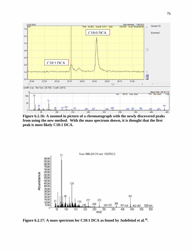
76
Figure 6.2.16: A zoomed in picture of a chromatograph with the newly discovered peaks
from using the new method. With the mass spectrum shown, it is thought that the first
peak is most likely C18:1 DCA.
Figure 6.2.17: A mass spectrum for C18:1 DCA as found by Judefeind et al.36.
C18:0 DCA
C18:1 DCA

77
Lastly, all of the calibration curves used for determining the concentrations of broth
components in the production study are presented in Figures 6.2.18, 6.2.19, 6.2.20, and 6.2.21.
Figure 6.2.18: Calibration curves for methyl oleate using both internal standards, PME
and HME.
Figure 6.2.19: Calibration curves for oleic acid using both internal standards, PME and
HME.
y = 7.0419x - 0.6139R² = 0.8822
y = 9.9418x - 0.6004R² = 0.8992
0.0
1.0
2.0
3.0
4.0
5.0
6.0
0.0 0.1 0.2 0.3 0.4 0.5 0.6 0.7
Are
a MO/A
rea I
S
Methyl Oleate Concentration (g/L)
PME
HME
y = 6.7999x + 0.8192R² = 0.6661
y = 13.958x + 0.5389R² = 0.9147
0.0
1.0
2.0
3.0
4.0
5.0
6.0
7.0
8.0
9.0
10.0
0.0 0.1 0.2 0.3 0.4 0.5 0.6 0.7
Are
a OA/A
rea I
S
Oleic Acid Concentration (g/L)
PME
HME

78
Figure 6.2.20: Calibration curves for stearic acid using both internal standards, PME and
HME.
Figure 6.2.21: Calibration curves for C18:0 DCA using both internal standards, PME and
HME.
y = 8.562x - 0.7991R² = 0.9528
y = 13.202x - 1.0962R² = 0.9656
0.0
1.0
2.0
3.0
4.0
5.0
6.0
7.0
8.0
0.0 0.1 0.2 0.3 0.4 0.5 0.6 0.7
Are
a OA
/Are
a IS
Stearic Acid Concentration (g/L)
PME
HME
y = 1.8164x + 0.0606R² = 0.6457
y = 3.5203x + 0.0197R² = 0.827
0.0
0.5
1.0
1.5
2.0
2.5
3.0
0.0 0.1 0.2 0.3 0.4 0.5 0.6 0.7
Are
a DC
A/A
rea I
S
C18:0 DCA Concentration (g/L)
PME
HME

79
6.3 LCDCA Production Studies
Examples of three separate cultures grown within the same trial are illustrated in the
following figures. The results presented in Figure 6.3.1 are for a control flask given 10 g/L of
glucose, while Figures 6.3.2 – 6.3.5 are for biological replicates given 10 g/L of glucose and 10
g/L of methyl oleate. Methyl oleate is not present at 0 hours of biotransformation in those
figures due to the fact that the cultures were sampled before the feedstock was added on that day.
The DCA denoted in the legends of each graph is the saturated C18:0 DCA since there were no
calibration curves produced for the unsaturated C18:1 DCA. Figures 6.3.1, 6.3.2, and 6.3.3 are
constructed using data from the GC-MS, while Figures 6.3.4 and 6.3.5 are constructed using data
with the HPLC method. These graphs will be compared in Section 7.3 in order to explore the
validity of the analytical methods.
Figure 6.3.1: The change in concentration of four key components over time measured by
GC-MS in Flask RCA, a control which was given 10 g/L of glucose for the co-substrate and
no feedstock. At 24 hours, there appears to be a considerable amount of C18:0 DCA
produced, but this trend was observed for all samples tested that day, indicating a possible
issue with standard carryover.
0.0
1.0
2.0
3.0
4.0
5.0
6.0
7.0
8.0
9.0
10.0
0 20 40 60 80 100 120
Co
nce
ntr
atio
n (
g/L
)
Biotransformation Time (hr)
OA DCA MO SA
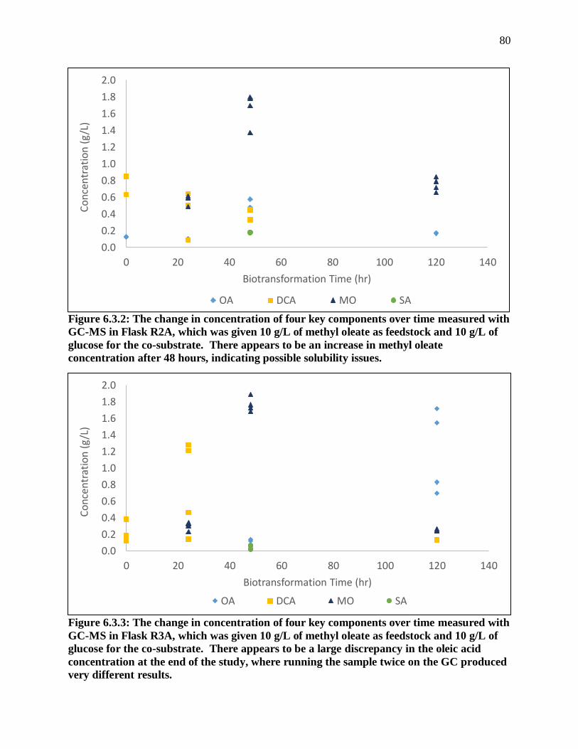
80
Figure 6.3.2: The change in concentration of four key components over time measured with
GC-MS in Flask R2A, which was given 10 g/L of methyl oleate as feedstock and 10 g/L of
glucose for the co-substrate. There appears to be an increase in methyl oleate
concentration after 48 hours, indicating possible solubility issues.
Figure 6.3.3: The change in concentration of four key components over time measured with
GC-MS in Flask R3A, which was given 10 g/L of methyl oleate as feedstock and 10 g/L of
glucose for the co-substrate. There appears to be a large discrepancy in the oleic acid
concentration at the end of the study, where running the sample twice on the GC produced
very different results.
0.0
0.2
0.4
0.6
0.8
1.0
1.2
1.4
1.6
1.8
2.0
0 20 40 60 80 100 120 140
Co
nce
ntr
atio
n (
g/L
)
Biotransformation Time (hr)
OA DCA MO SA
0.0
0.2
0.4
0.6
0.8
1.0
1.2
1.4
1.6
1.8
2.0
0 20 40 60 80 100 120 140
Co
nce
ntr
atio
n (
g/L
)
Biotransformation Time (hr)
OA DCA MO SA

81
Figure 6.3.4: The change in concentration of four key components over time measured by
HPLC in Flask R2A, which was given 10 g/L of methyl oleate as feedstock and 25 g/L of
glucose for the co-substrate. Samples at all time periods were tested once and
concentrations were estimated with refractive index detection and absorbance detection at
210 nm. There still appears to be an increase in methyl oleate concentration at 48 hours,
and there is no product formed throughout the trial.
Figure 6.3.5: The change in concentration of four key components over time measured with
HPLC in Flask R3A, which was given 10 g/L of methyl oleate as feedstock and 10 g/L of
glucose for the co-substrate. Samples at all time periods were tested once and
concentrations were estimated with refractive index detection and absorbance detection at
210 nm. There appears to be no consistent consumption of methyl oleate and no product
formed throughout the trial. There is a slight discrepancy in the oleic acid concentration at
120 hours.
0.0
1.0
2.0
3.0
4.0
5.0
6.0
7.0
8.0
9.0
0 20 40 60 80 100 120
Co
nce
ntr
atio
n (
g/L
)
Biotransformation Time (hr)
OA DCA MO SA
0.0
1.0
2.0
3.0
4.0
5.0
6.0
7.0
8.0
9.0
10.0
0 20 40 60 80 100 120
Co
nce
ntr
atio
n (
g/L
)
Biotransformation Time (hr)
OA DCA MO SA

82
7. DISCUSSION
7.1 Optimal Carbon Substrate for Growth of C. viswanathii
Before the results are analyzed, the substrate concentration choices are first justified for the
study. Glucose is the simple sugar that most carbohydrates are broken down to in order to be
metabolized, so it is important to test the yeast growth on this substrate to compare to others as
an industrial standard. The concentration of 30 g/L was chosen based on what Mobley used in
his OPT1 medium recipe11. In order to keep the volume across cultures constant, stock solutions
for glycerol and xylose were made so that 5 mL could be added to give the same concentration.
This was easily done for glycerol; however, xylose had a much lower solubility in water. Once
dissolving the xylose became difficult even after heating up the solution to 60°C, the
concentration was left at 150 g/L, translating to a concentration of 25 g/L in the media.
When mixing glucose with either glycerol or xylose, it was thought that keeping a higher
concentration of glucose would help to keep the growth rate high initially, due to the yeast
preferentially consuming the glucose first. The glucose would run out after 12 hours or longer,
but before the 24-hour time limit given in this study. In this case, it was believed that the biomass
concentration after glucose was consumed would be high enough that once 24 hours of growth
was reached, the final biomass concentration after metabolizing the other substrate would still be
comparable to the value obtained on pure glucose. An optimal growth phase would reach the
stationary growth phase in a shorter time span and leave the largest biomass concentration for the
initiation of the production phase, so these mixtures have the potential to compete with pure
glucose in both categories and also cut down the cost of the feedstock. It was thought that a ratio

83
of 3:1 glucose to xylose or glycerol might not have been very cost effective, but a ratio of 1:1
would not be as effective in reaching a higher final biomass concentration. Therefore, a ratio of
2:1 was chosen to be a good compromise between the two qualities.
For glycerol, it is not well documented what the highest concentration should be when
growing C. viswanathii, so 30 g/L could have been too high and caused many issues with culture
growth. Throughout the study, it was found that cell cultures were more prone to dying when
glycerol was used as the carbon source. When comparing the initial and final concentrations of
glycerol during the growth studies, only about 60% of the substrate was used on average, where
the other substrates were completely metabolized after 24 hours. Glycerol was added with the
same mass concentration; however, it was added at twice the molar concentration of xylose and
glucose. This could have led to issues with cell lysis resulting from an increase in osmotic
pressure, which is dependent on the number of molecules and not their cumulative mass.
Another issue was that the metabolism of glycerol required more oxygen for the concentration
that was given. To completely oxidize a molecule of glucose, six molecules of oxygen are
required. Xylose requires at least 5 molecules and glycerol requires 3.5 molecules of oxygen.
Since the number of glycerol molecules added was doubled, that would mean that 7 molecules of
oxygen would be required for each glycerol molecule to be metabolized. This could have led to
oxygen limitations occurring more rapidly in the cultures. More research should be done to look
at reducing the concentration of glycerol added by half to be more cost effective and increase cell
viability.
Another issue encountered was the accuracy of the YSI bioanalyzer used to monitor
substrate concentration. When measuring higher concentrations, the bioanalyzer had a precision
around ±2% and a linearity of about ±5%. Based on linearity alone, an initial concentration of 30

84
g/L could vary from about 28.5 g/L to 31.5 g/L when measured. The system would attempt to
reduce this variability by regularly recalibrating itself after every 10 samples. However, as the
membrane activity and sensitivity decreased, the values obtained for concentration would tend to
decrease as well with time, so calibration standards were used often to create calibration curves
for after each recalibration. Even with this calibration method in place, there would still be quite
a bit of scatter in the data, especially for flasks where the concentration of substrate was not
expected to change much, like when using a secondary substrate in the glucose mixtures. That is
how negative values can be seen for consumption rate, particularly in the first few hours of
growth, where the concentrations are at their highest. Using statistical modeling may help to
account for the variability over time in the samples, but another method for measuring substrate
concentration should be considered to obtain more accurate values of biomass yield coefficients.
Even with these limitations, there are clearly substrates that have much higher specific
growth rates and yield coefficients than others. As expected, growth on glucose gives the
highest specific growth rate of 0.482 ℎ𝑟−1 comparatively to xylose at 0.460 ℎ𝑟−1 and glycerol at
0.417 ℎ𝑟−1. To put these values in perspective, after 12 hours of exponential growth, the
biomass concentration on glucose would be more than double of that on glycerol. On the other
hand, the biomass yield coefficient on glucose was determined by the statistical analysis to be
about 0.754 g of biomass dry cell weight produced per g of substrate consumed, which is much
lower than the values estimated for glycerol and xylose, which are 1.420 and 1.600 respectively.
To compare the above values to literature, Candida utilis was found to grow on glucose
with a specific growth rate of 0.45 ℎ𝑟−1 and a biomass yield coefficient of 0.51 g/g according to
Shuler et al38. These values seem comparable to what was found in this study, considering that
the yeast extract contributed to an increase in the biomass yield coefficient. Funk et al. found

85
conversely that in a batch configuration, their specific growth rate on glucose using C. tropicalis
was 0.14 ℎ𝑟−1 and their biomass yield coefficient was 0.44 g/g. They explained that their values
were much lower than they theoretically should have been most likely due to ethanol formation1.
It is possible that ethanol formation occurred in this study, but the concentration was not tested.
An HPLC method is recommended to be used to determine the ethanol production with time and
account for it in the regression model.
When considering that the growth parameters with glucose are reasonable, the values
obtained for glycerol make sense from a theoretical standpoint, but the biomass yield coefficient
for xylose does not. Theoretical values of the biomass yield coefficients can be calculated using
a relationship presented by Shuler et al., which involves the number of oxygen molecules
required for complete reduction of each substrate and a relative estimate for biomass formed for
each electron accepted based on using ammonia as the primary source of nitrogen38. This
calculation results in biomass yield coefficients of 0.419 g/g for both glucose and xylose and
0.478 g/g for glycerol. First, this contradicts what was observed with xylose being similar to
glycerol in terms of the biomass yield coefficient. Secondly, this shows that glycerol should
have a higher value, even though the value determined in the statistical analysis is double that of
glucose. That could occur due to oxygen limitations, where glycerol would no longer be
metabolized, but the carbon sources within the yeast extract would be depleted. Xylose should
still be similar to glucose though, since they are both fermentable in anaerobic conditions.
One possibility for why the xylose biomass yield coefficient is much larger than expected
is that more ethanol was produced when glucose and glycerol were used as substrates, reducing
their apparent coefficient values. However, this is unlikely since the glucose yield coefficient
did not deviate from literature and theoretical values nearly as much as xylose. In order to

86
visualize another potential issue, the biomass yield coefficients were numerically estimated with
two different methods for comparison to the model. First, the biomass yield coefficients were
determined by comparing the biomass and substrate concentrations between 2 and 10 hours of
biotransformation, as shown in Table 6.1.2.1. It was found that the biomass yield coefficient
with xylose was still double that obtained with glucose. Secondly, the initial values and final
values after 24 hours were used to calculate the biomass yield coefficients, which are presented
with the final biomass concentrations in Table 6.1.2.2. Here it can be determined that xylose
produced a biomass yield coefficient of 0.563 g/g that was more comparable to glucose, which
produced a maximum value of 0.323 g/g. Glycerol resulted in a biomass yield coefficient that
was still more than double that of glucose. With these significant differences in the calculated
xylose biomass yield coefficient, it is possible that there was a considerable amount of error in
the substrate consumption rates. Since there was such a small change in xylose concentration
before 10 hours, the uncertainty in the YSI membrane contributes significantly to the results of
the statistical model and the first numerical method. The second numerical method may provide
a more accurate estimate, but a different analytical method should be devised to verify that.
More data should be collected within the 24 hour time period as well in order to make a
conclusive decision on the length of the lag period, since it is unknown with just 12 hours of data
recorded, and calculate new biomass coefficients based off of the start and end of the exponential
phase of growth.
For the substrate mixture trials, the results do not exactly match with what was predicted.
Since the yeast should preferentially metabolize the glucose first, the growth rates and the
biomass yield coefficients on glucose in the mixtures should be similar to that of pure glucose.
However, the trials conducted had much lower specific growth rates at 0.405 ℎ𝑟−1 for the

87
glucose and glycerol mixture and 0.386 ℎ𝑟−1 for the glucose and xylose mixture, and also had
different yield coefficients at 0.547 for the glucose and glycerol mixture and 1.230 for the
glucose and xylose mixture. The difference in these results could be explained by the fact that
these trials were most likely not kept at a constant temperature as they should have been.
Growth on pure glucose was mainly tested in the winter quarter, where the heating units were
turned on to keep the labs warm, while growth on the mixtures was recorded in the spring
quarter, before the air conditioning units were gradually turned on. The incubators used had
mechanisms for heating but not cooling, so they would sometimes overheat and the temperature
would go up to as high at 31.4°C. Efforts were made to move the system to the center of the lab,
away from the refrigerators and other equipment, and where the exhaust would not be obstructed.
These efforts did not stop the problem from occurring. In consequence, when comparing the raw
data for growth on pure glucose and the mixtures, it would appear that the initial biomass
concentration was much higher for the mixture trials, when in reality they should have been the
same. This probably affected the regression model and caused the data for the mixture trials to
have much lower specific growth rates, as opposed to if the initial biomass concentration would
have been fixed in the model. The determination of the specific growth rates then affected the
determination of the biomass yield coefficients, since the regression model used then included
the estimated specific growth rates calculated with the other model.
Some visual evidence that contradicts the statistical regression for the specific growth
rate can be seen in Figures 7.1.1 and 7.1.2. Each figure represents the cultures grown in the
same trial in the spring quarter. Notice that the starting biomass concentrations and specific
growth rates are similar within each plot. The temperatures differed between the trials in Figures
7.1.1 and 7.1.2, so they are not comparable, but the data can be compared within each trial. In
88
Figure 7.1.1, the flasks containing glucose had similar specific growth rates to the flasks
containing glucose and xylose. Then by extension, if the specific growth rates between the
cultures grown on glucose and xylose mixtures and glucose and glycerol mixtures are similar in
Figure 7.1.2, then the specific growth rate on glucose would likely be comparable to the specific
growth rate on the glucose and glycerol mixture too. Since the regression model does not
account for temperature or the different quarters in which data was taken, there are some
limitations on how the results could be interpreted. With the logic above, it can be concluded
that even though the statistical regression model states that growth on glucose and xylose
mixture is significantly different (p-value < 0.05) than that of glucose, the results may not be
statistically valid as temperature was not consistently maintained and was unaccounted for in the
model. When comparing glucose to the other trials though, those results may still be valid as
xylose and glycerol were tested together in the winter, where the temperature in the lab was
believed to fluctuate less. Under that assumption, it was found that specific growth rate of C.
viswanathii on glucose was statistically different than the values for glycerol and xylose. No
statistical inferences can be made about the biomass yield coefficients though due to the
elimination of variability in the model by directly including the specific growth rates calculated
with another model in the regression. If the specific growth rates were allowed to vary, then
statistical inferences could have been made.

89
Figure 7.1.1: Growth curves of C. viswanathii studied on 4/18/18 in the spring quarter with
glucose or a glucose and xylose mixture for the carbon substrate.
Figure 7.1.2: Growth curves of C. viswanathii studied on 4/11/18 in the spring quarter with
a glucose and glycerol mixture or a glucose and xylose mixture for the carbon substrate.
y = 0.0802e0.4244x
y = 0.0864e0.4148x
y = 0.0886e0.4163x
y = 0.0707e0.4514x
y = 0.0871e0.4206x
y = 0.0864e0.4186x
0.0
0.5
1.0
1.5
2.0
2.5
3.0
3.5
4.0
4.5
5.0
0 1 2 3 4 5 6 7 8 9 10
Cell D
ensity, g D
CW
/L
Time Elapsed, hr
Glucose,Flask 1
Glucose,Flask 2
Glucose,Flask 3
GluXy,Flask 4
GluXy,Flask 5
GluXy,Flask 6
y = 0.0809e0.4896x
y = 0.0775e0.4856x
y = 0.0802e0.4927x
y = 0.0798e0.4907x
y = 0.0742e0.5064x
y = 0.0727e0.5102x
0.0
1.0
2.0
3.0
4.0
5.0
6.0
0 1 2 3 4 5 6 7 8 9 10
Cell D
ensity, g D
CW
/L
Time Elapsed, hr
GluGly,Flask 1
GluGly,Flask 2
GluGly,Flask 3
GluXy, Flask1
GluXy, Flask2
GluXy, Flask3

90
Deciding which carbon substrate is optimal for the growth of C. viswanathii depends on a
number of factors, which revolve around how the process is designed. If the process is to be an
extension to a pre-existing ethanol plant, as in the report by Busch et al., then capitals costs are
minimal and the number of unit operations can be reduced, allowing the utilities and production
costs associated with maintenance and labor to be less expensive than the feedstock cost. More
significant contributions to cost reduction could be achieved by using a cheaper carbon substrate
or a byproduct of the connecting plant for substrate. One of the reasons why the designed add-on
process was deemed significantly profitable was because the glycerol obtained from the
transesterification of corn oil was repurposed as the carbon substrate in the fermentation step13.
In some grassroots plants, like designed by Mobley in the feasibility report for General Electric,
the feedstock price can still far outweigh the price of utilities and equipment maintenance, where
64% of the total production cost in this particular case was from chemicals used in the process.
Of the chemical expenses, about 37% was from purchasing the methyl myristate feedstock, but
there was no description of the composition of the rest of the chemical inventory list11. It can be
assumed that the carbon substrate and media still takes up quite a bit of the cost, since the other
chemicals used in the process were strong acids, bases, and solvent. However, for processes like
this where there is no ability to use a byproduct for a carbon substrate, a more extensive
economic analysis should be done to determine if there would be more of a cost advantage to
grow up the yeast cultures faster and increase the total throughput of LCDCAs with a more
expensive substrate such as glucose, or reduce the feedstock cost by using cheaper glycerol or
xylose produced by another facility.

91
7.2 Analytical Method Improvements and Contributions to Literature
The initial analytical approach in this study was modeled after the work presented in a
dissertation by Nina Rimmel from the Technical University of Munich31. Her work provided the
foundation for the ratios of chemicals used in the extraction and derivatization steps and the
starting conditions for the GC analysis. The parameters in her methods and her justifications for
using them will be contrasted to the changes that were made in the protocol for this study,
summarized in Section 6.2, and the limitations of this improved method will be explained
further.
7.2.1 Alterations to the Extraction Protocol
The first method that will be compared is the extraction of the production samples.
Extraction is necessary to prevent damaging the low polarity polysiloxane column with the
presence of water and to avoid interference from other metabolites present in the aqueous broth.
The goal was to remove the majority of the water-soluble impurities present in the supernatant
and transfer the components of interest into an organic solvent suitable for gas chromatography
in a single step. Extraction into MTBE was chosen since the solvent was compatible with all of
the LCDCAs and other low polarity components present in the broth. As another requirement, it
also lacks any free hydroxyl groups that could be derivatized by MSTFA in the subsequent step.
Rimmel further explains that MTBE is less toxic and volatile that diethyl ether, which was used
in other literature resources for a similar extraction with fermentation broth31.
The extraction protocol that Rimmel followed involved taking 500 µL broth samples and
adding 200 µL of 1 N HCl and 1000 µL of MTBE. The microcentrifuge tubes used in this study
could not quite contain this amount of liquid, which is why the sample size taken was scaled
92
down to 400 µL, with the 1 N HCl and MTBE being scaled down to 160 µL and 800 µL
accordingly. Rimmel would thoroughly mix the immiscible liquids and then place the tubes on a
shaker for 2 hours and then repeat the process again in a multistage extraction31. In order to
ensure equilibrium is obtained without having to do multiple steps, the tubes are shaken for 3
hours instead in this study. This method reaches a recovery of approximately 71%-72%, which
was determined in a study where methyl oleate standards were made in broth before extraction,
in MTBE before derivatization, and in MTBE without derivatization to see the relative
differences in concentration. The yield determination is explained in Section 6.2, where Figure
6.2.1 illustrates the relative difference in GC peak area for samples undergoing both extraction
and derivatization and samples that undergo neither. The last extraction parameter, the vortex
shaker setting, was chosen due to it being a compromise between thorough mixing of the
samples and less movement of the shaker itself.
7.2.2 Alterations to the Derivatization Protocol
Derivatization was originally modeled after Rimmel’s protocol and was later slightly
altered after finding new techniques in similar studies. MSTFA was used by both Rimmel and
Funk et al., another group of researchers who used a similar analysis protocol, for the
derivatization reagent1,31. By converting the carboxylic acid ends to TMS ends, the polarity of
the compound is reduced, making it more suitable for separation using the polysiloxane column.
TMS derivatives also aid in the characterization of the compounds using mass spectrometry,
since they produce fragments that have more unique m/z ratios. MSTFA in particular is one of
the most volatile TMS derivatization reagents and can derivatize more volatile components,
which helps to determine if there are smaller chain DCAs and FFAs in solution. Some of the
93
drawbacks of using a derivatization reagent for TMS derivatives include the reagent and the
derivatized compounds increased sensitivity to water and excessive heat. Artifact peaks can also
appear in gas chromatographs due to the incomplete reaction or breakdown of the TMS
derivatives53.
In this study, artifact peaks commonly occurred, and some specific examples can be seen
in Figures 6.2.12, 6.2.13, and 6.2.14. Figure 6.2.12 shows what happens if the injection
temperature causes breakdown of multiple TMS derivatives. Figure 6.2.13 shows some
unknown components that are believed to be breakdown products of the C18 DCAs studied due
to their long retention time. Figure 6.12.14 shows the most common artifact occurrence. A
small peak appears at the same retention time as the C18:0 DCA, but is not identified by the
NIST library to be that component. The suggestions that the similarity search gives are
commonly siloxanes or random silyl conglomerates. This peak was also found to appear when
pure MSTFA in MTBE was injected into the column. Although there is not a lot of evidence to
support this hypothesis, the current leading theory is that this artifact peak is actually C18:0 DCA
that was stuck on the column, but just in such a small quantity that the characteristic m/z values
do not show up in high enough intensities to warrant a conclusive decision on the identity of the
compound in the NIST library. While it is certainly possible that this artifact peak is something
different entirely, it is most likely some derivative of the C18:0 DCA due to the fact that the
characteristic m/z values do appear occasionally in the mass spectra and the retention times line
up closely.
There are also some additional challenges associated with using MSTFA for derivatization.
First, the shelf life of MSTFA is only about one month, after which it does not derivatize
components with the original yield. Secondly, MSTFA breaks down the rubber stoppers used in

94
syringes to pull suction on samples, which can cause the amount of MSTFA added to vary
significantly when the syringe gets stuck over time. Syringes were replaced after 6-10 uses on
average in an attempt to avoid this problem. MSTFA breaks down in air naturally due to the
presence of water vapor, so the MSTFA bottles were kept under a nitrogen purge. This may not
have been very effective though since air would still get sucked into the bottle after the syringe
was removed and before the nitrogen could be added, further reducing the shelf life. Possible
alternative derivatization reagents for LCDCAs have been considered, but most literature sources
utilize TMS derivatives. It would be possible, however, to investigate whether it would be more
efficient to convert the product and FFAs to their ethyl ester derivatives via transesterification
prior to analysis on the GC-MS. Methyl esters were being selected for feedstocks in this study,
but it is possible to use ethyl esters as well. However, if methyl esters were selectively used for
the biotransformation, then derivatizing the acid components into ethyl esters would lead to
entirely unique peaks on the GC-MS. The major downside to this argument is that there is
currently no research on the boiling points of the ethyl ester equivalent of C18 LCDCAs, at least
with what was reviewed previously, so there is a possibility that the boiling point would still be
too high for a polysiloxane column like what was used in this study. Another approach would be
to remove the derivatization step entirely and use an HPLC column to test purified broth samples
such as a method that Rimmel had developed31.
Several method changes were explored in order to increase the MSTFA conversion of
components in the organic extraction phase and take preventative measures against water
contamination. In the original method by Rimmel, 250 µL of the organic phase were transferred
from the final extraction solution to GC autosampler vials. To each extracted sample, 500 µL
MTBE was added to further dilute the samples, and then 50 µL N-methyl-N-

95
(trimethylsilyl)trifluoroacetamide (MSTFA) was added to derivatize them. Although the
MSTFA was known to be in significant excess on a molar basis, with a MSTFA to sample ratio
of about 67.5:1 to 135:1, other research articles suggested that larger values of excess could help
keep the reaction yield consistent while mitigating the effects seen from various sources of
reactant degradation. For example, Basconcillo and McCarry used an excess as large as 500:1
MSTFA to total fatty acid composition to ensure that their method worked54. In the results of a
study presented in Figures 6.2.4 and 6.2.5, it was found that adding 100 µL MSTFA greatly
improved the calibration curves with respect to the internal standards used, which are discussed
in more detail later in this section. In order to reduce the amount of MSTFA due to economic
reasons, the sample volume was reduced by half, along with the internal standards that were
added. This allowed the MSTFA to be in excess with a ratio of 135:1 to 270:1.
Before derivatization began, the addition of pyridine was investigated as an alternative to
drying the samples before placing them on the GC, since there was no drying step in the original
method. Magnesium sulfate was used a drying method for the samples in the study by Fabritius
et al.19. Alternatively, Sigma-Aldrich suggested using blowing nitrogen gas over the top of the
samples55. Many other analytical-based literature articles included pyridine in their reaction
mixture, including the studies by Basconcillio and McCarry, Judefeind et al., and Cho et al35,36,54.
In particular, Cho et al. found that the optimum ratio of MSTFA to pyridine was 9:1 in order to
help prevent hydrolysis of samples and still have high-resolution chromatographs35. The ratios
of 4:1 and 6:1 were studied in order to see if there was any significant impact on the amount of
pyridine added. These ratios were partly chosen due to the fact that the C18:0 DCA standard
was dissolved in pyridine and the standard was quite concentrated at 30 g/L. In order to mimic
extracting a high concentration of 3 g/L in broth, the ratio of 4:1 was the smallest possible ratio

96
that could be done so that all of the pyridine added to the control came from the C18:0 DCA
stock solution. With these ratios studied, it is clear from Figure 6.2.6 that the calibration curves
for C18:0 DCA were not significantly worse for either case. However, even though there
appeared to be slightly more sensitivity in the 6:1 samples from the larger slope produced, the
4:1 ratio was chosen to be used throughout the production study so that the stock solution of
C18:0 DCA would not have to be remade.
As for the heating time and temperature for the samples, neither Rimmel or Funk et al. had
reported heating the samples to obtain a better yield1,31. However, Cho et al. found that
derivatizing for one hour at 60°C was effective at allowing the reaction to complete35. This
study started with derivatizing the LCDCAs and other components at 60°C for three hours, but
then explored reducing that time while still keeping a high enough conversion to produce
consistent data for calibration curves. It was believed that at some point in the study, the methyl
oleate standards were breaking down with the excessive heating, and that there was also a
possibility for the oleic acid and DCAs to degrade or turn into their trans isomers. In the
experiments conducted by Basconcillio and McCarry, they found that heating their C14:0 fatty
acid methyl esters for 15 minutes at 50°C and 60°C resulted in poor recoveries compared to
heating the same standards for 15 minutes or longer at 25°C. These results were not due to
hydrolysis, as there were minimal changes in the concentration of C14:0 fatty acid TMS
derivatives in the samples. They concluded that it is possible that a type of condensation
reaction could be occurring at the higher temperatures54. Contrary to their argument, Cho et al.
and Judefeind et al. found that they were able to derivatize their samples for an hour each at
60°C and 75°C respectively with no noticeable breakdown or creation of new components or
artifacts35,36. In order to experiment with the changes in the recovery in this study, the

97
derivatization time was changed to 20, 40, and 60 min. The component studied was C18:0 DCA
rather than methyl oleate though since it was a priority to derivatize as much of the DCA as
possible. In Figure 6.2.7, it was found that 20 minutes of derivatization at 60°C would be
enough time to produce acceptable calibration curves, which considerably reduced the time
needed to prepare samples in the laboratory.
In addition to the reduction in heating time, internal standards and MTBE were not added
to dilute the samples prior to derivatization, because it was thought that it would decrease the
yield if the sample was not thoroughly heated. Once the derivatization reaction was complete,
463 µL MTBE was added to each sample to further dilute the concentration, because the
reported protocol from Rimmel was appropriate for concentrations between 0.25 and 15 mM31.
The internal standards were added along with the MTBE to achieve a concentration of 0.5 g/L,
which was calculated to be 25 µL of a 2.6 g/L stock solution for each.
7.2.3 Identification of the Unsaturated DCA Product with GC-MS
The original method for analyzing LCDCAs with GC-MS used in the Rose-Hulman
Laboratory was created by a former student, Katie Ryan. She attempted to adopt the methods
present in Rimmel’s dissertation, but found that they were not completely reproducible for the
column used for this research. Another major setback was that both Rimmel and Funk et al. used
flame ionization detectors (FID), but the column setup for this experiment had mass
spectrometry available instead1,31. Using an MS enabled system does have a significant benefit
compared to FID systems, where fouling of the detector via silica accumulation can be more
easily avoided53. Determining the parameters for mass spectrometry was more difficult due to
lack of literature present with a MS protocol. According to the National Institute of Standards

98
and Technology (NIST) library within their Chemistry WebBook56, the TMS derivative of
octadecanedioic (C18:0) acid has a characteristic m/z value of 443. Since this is the largest
LCDCA of interest, it was assumed that all of the other LCDCAs and FFAs would have
characteristic m/z values below 443, so the range of m/z values tested for was 25 to 450. A
simple scan mode was utilized instead of selective ion monitoring (SIM) due to lack of
knowledge of the m/z values of other components in the fermentation broth.
It was later found in the article by Judefeind et al. that they had obtained a mass spectra
for the C18:1 DCA that is produced in this study, shown in Figure 6.2.17 with a characteristic
m/z value of 44136. Figure 6.2.16 shows the new peaks that were obtained from a production
study, of which the early eluting one is assumed to be the monounsaturated C18 DCA of interest.
The adjacent peak is thought to be either the trans isomer of the C18:1 DCA or a translocation of
the double bond. A mass spectra of the first peak is shown below the chromatograph to show
how it lines up with what Judefeind et al. found. Note that these peaks only started appearing
after all of the above changes were made to the extraction and derivatization method.
7.2.4 Implementation of Internal Standards
Another motivation for changing the GC method was that the calibration curves that
Katie had made could not be recreated after a few months of testing, and it was assumed that
something had changed with the column or how it operated. The original method was used to
determine if there were repeatability issues with using the column. It was found that when four
different standards of methyl oleate, which had not been extracted or derivatized, were
repeatedly sampled on the column, there was always either a high or a low value for the peak
integration, as shown in Figure 6.2.2. A single sample of 0.48 g/L of technical methyl oleate
99
stock was repeatedly sampled overnight to see if the same phenomena occurred again. The
results presented in Figure 6.2.3 were quite unusual, where not only did the phenomena occur for
the methyl oleate component again, but it occurred for all of the impurities that were present in
the technical grade solution as well. After consulting with professors in the chemistry
department and the technician, the only logical reasons behind how this phenomenon could occur
would be if there was something malfunctioning with the syringe that would cause it to stick at
times, or if there was a consistent fluctuation in temperature. To make sure there was no residue
built up in the syringe and the injection port for the rest of the production study trials and
analytical development, they were both promptly replaced. When removed, the glass liner was
observed to have a large black mass stuck in the center, which had never been witnessed with
this instrument before. It was thought that it may have been caused by some of the heavy boiling
components not being completely volatized when injected, and was assumed to have been partly
to blame for the inconsistencies seen in injection volume.
In order to ensure that injection volume would not cause significant variation in the
calibration curves and production study results again, it was decided to start using internal
standards. The idea behind internal standards is that they are consistently added at the same
concentration, so that if the injection volume changes, the peak integration could change with it
while keeping the ratio between the internal standard and the other components constant.
Calibration curves can then be made with respect to these ratios instead of total peak area. The
internal standards used in a study must be similar in structure and boiling point to the
components in the solution, so that they would appear with high resolution on the
chromatographs in the temperature range that is being tested. For example, the use of ethyl
dodecanoate as an IS in the study by Basconcillio and McCarry would not be compatible with

100
this study, since it would most likely have a much lower boiling point than the other components
derived from the fermentation broth due to its much lower chain length (C12). Methyl
pentadecanoate (PME, C15:0) and methyl heptadecanoate (HME, C17:0) were chosen for this
study because not only are they similar in chain length to the C16 and C18 components that are
expected to appear in corn oil, but they also have odd-numbered chain lengths, which do not
occur often by natural metabolism in yeast. These components would not be expected to appear
in fermentation broth under any circumstances.
7.2.5 Adjustment of GC Injection Volume and Temperature
Even with the use of internal standards, sometimes the chromatographs would not be very
clear or would have very minute peaks. Figure 6.2.9 represents a sample that was tested at the
original injection temperature of 275°C. The internal standard peaks are barely visible and are
not significant enough to integrate. It was thought that maybe the injection temperature was
either too high and was breaking down the components or too low and was not vaporizing them
to a large extent. For another sample that had experienced the same problem, injection
temperatures of 200°C and 300°C were tested along with the original specification. The low
bound of 200°C was chosen because of the recommendation from Restek to avoid breakdown of
TMS derivatives51. However, it was found that there was a large solvent front produced that
completely obscured all of the other peaks that should have been present. On the other hand,
when a higher value such as 300°C was used, the resolution of the peaks increased and the
baseline remained flat. It was found that after testing all of the production samples once at
275°C and once at 300°C that although increasing the temperature did not always improve the
baseline, it did not seem to break down the derivatives to a significant degree. For example,

101
Figure 6.2.10 represents the same sample that was tested in Figure 6.2.9, but shows two
chromatographs taken with the same injection temperature of 300°C. The first trial did produce
larger peaks, but it was not as clear as the second trial, which had a much flatter baseline. A
good example of a chromatograph taken with the higher injection temperature is shown in Figure
6.2.11, where the peaks are clearly defined and there is no baseline noise.
With these examples, it should be noted that the internal standards did not always explain
the change in the peak areas or the appearance of new peaks with the clearer chromatographs.
That leads to the thought that there might be something else inherently wrong with the column.
A possibility is that there is an inconsistency in the injection temperature. That would explain
how the chromatographs look completely different for the same temperature even if the samples
are tested at the same injection temperature. There were many cases were the chromatograph of
a sample injected at 275°C would look exactly like the chromatograph when it was injected at
300°C. Also, if injection volume were to blame, the sudden appearance of peaks would not
occur, especially when the relative IS peak area did not change. There was not an easy way to
check if the injection temperature reported in the system was accurate, especially since the
instrument was being used by many people at the time. However, it was less invasive to measure
the oven temperature, and the thermocouple reading was found to be within ±3°C of the
indicated temperature during the entire ramp period. It is suggested that the injection
temperature be measured during the next scheduled time for routine maintenance of the injection
port. If a discrepancy arises, it would be worth the effort to look for a more insulted liner for
future studies, especially since the temperature down the length of the liner can vary anywhere
from 20°C to more than 100°C within a study of multiple Agilent split/splitless liners57.

102
Another issue that may have been occurring with the initial GC-MS method was
excessive back flash of the samples when injected. This may have been a partial cause of the
observed injection volume inconsistencies since a small sample concentrations would have led to
much easier volatilization of the solvent in the injection port. Katie had used a large injection
volume for her method development because it resulted in larger, more defined peak areas for the
components that she tested. However, when a solvent expansion calculator was used on the
Restek website, it was found that excessive back flash was occurring. The volume of vapor
produced was twice as large as the available volume within the injection liner. In Figure 6.2.8,
the calculator was used to determine that the maximum injection volume should be around 2.2
µL to prevent any back flash. To be conservative, the injection volume was rounded down to 2
µL for analyzing the production study samples.
Lastly, when controls for C18:0 DCA were run in the same batch as unknown samples, it
was thought that sometimes the LCDCA would get stuck on the column. The original method
had no fast boiling ramp at the end to remove high boiling impurities. Instead, it kept the final
temperature at 280°C for 5 minutes. Since the column should not be held at higher temperatures
for prolonged periods of time, a short ramp of 20°C/minute was added at the end to reach a final
temperature of 300°C which was held for 1 minute.
The final calibration curves for methyl oleate, oleic acid, stearic acid, and C18:0 DCA
used with this modified method are presented in Figures 6.2.18, 6.2.19, 6.2.20, and 6.2.21. Note
that Funk et al. had also focused on making calibration curves for C18 FFAs and the retention
times they witnessed were very similar, ± 6 seconds on average, to those obtained with this
protocol1. A complete summary of method changes is presented below in Table 7.2.1.

103
Table 7.2.1: Summary of all of the changes made in the analytical method for the
determination of FFA and DCA concentrations with GC-MS.
Parameter Original Method New Method
Extraction Volume
500 µL sample
200 µL 1 N HCl
1000 µL MTBE
400 µL sample
160 µL 1 N HCl
800 µL MTBE
Derivatization Volume
250 µL organic layer
500 µL MTBE
50 µL MSTFA
125 µL organic layer
12.5 µL pyridine
50 µL MSTFA
Max MSTFA Excess 135:1 270:1
MSTFA:Pyridine Ratio No pyridine added 4:1
Derivatization Time 3 hrs 20 mins
Internal Standards None
0.5 g/L of PME
0.5 g/L of HME
Injection Temperature 275°C 275°C or 300°C
Injection Volume 5 µL 2 µL
Temperature Ramp
Hold at 160°C for 5 min
Increase by 5°C/min until
280°C
Hold at 280°C for 5 min
Total Time: 34 min
Hold at 160°C for 5 min
Increase by 5°C/min until 280°C
Hold at 280°C for 5 min
Increase by 20°C/min until
300°C
Hold at 300°C for 1 min
Total Time: 36 min

104
7.3 Conditions for Relatively Highest LCDCA Yield
Before analyzing the results, the viability of the GC-MS method will be determined using
the data presented in Figures 6.3.1 – 6.3.5. From these figures, which contain data from cultures
grown in the same trial, it is apparent that three issues are observed with the method. The first
issue is illustrated in Figure 6.3.1, which records the concentrations of major feedstocks and
products as reported by GC-MS for a control flask. Note that no methyl oleate or oleic acid was
added to the flask; however, C18:0 DCA appears in the samples. The apparent concentration
was as high as 9 g/L, which is more than what was recorded for all of the other samples tested
across all trials. This raises concerns because there should not have been any DCA product
produced in the control. The fact that it is the saturated DCA that appeared and not the proposed
unsaturated product also indicates that the sample may have had C18:0 DCA carryover from the
standard that was run within the same autosampler batch. A standard containing methyl oleate
and C18:0 DCA was run with each batch on the GC-MS to ensure that the method was working.
All samples that were tested from 24 hours of biotransformation on that day all had high amounts
of C18:0 DCA according to the GC-MS results, further illustrating that carryover most likely
occurred due to the standard getting stuck on the column. Eventually, the C18:0 DCA peaks no
longer appeared in the chromatographs with the standards that were prepared and derivatized
each day, indicating that either the MSTFA had degraded or the column was not fully volatizing
the samples. This was the primary reason that the samples were then tested using an HPLC
method to obtain estimates for sample concentration and verify that C18:0 DCA peaks were
likely carryover from previous standards. The samples in Figures 6.3.2 and 6.3.3 also showed
C18:0 DCA peaks in the GC-MS analysis, but when they were tested with HPLC in Figures
6.3.4 and 6.3.5 respectively, there was no DCA standard found for all samples collected over
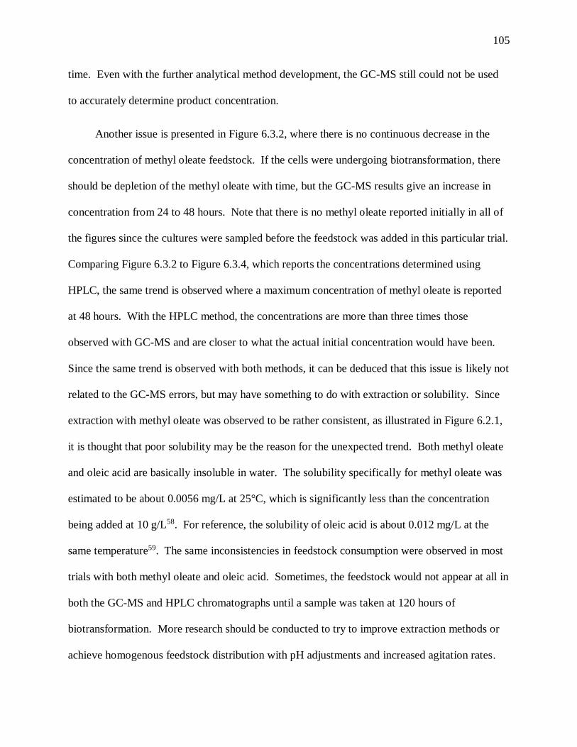
105
time. Even with the further analytical method development, the GC-MS still could not be used
to accurately determine product concentration.
Another issue is presented in Figure 6.3.2, where there is no continuous decrease in the
concentration of methyl oleate feedstock. If the cells were undergoing biotransformation, there
should be depletion of the methyl oleate with time, but the GC-MS results give an increase in
concentration from 24 to 48 hours. Note that there is no methyl oleate reported initially in all of
the figures since the cultures were sampled before the feedstock was added in this particular trial.
Comparing Figure 6.3.2 to Figure 6.3.4, which reports the concentrations determined using
HPLC, the same trend is observed where a maximum concentration of methyl oleate is reported
at 48 hours. With the HPLC method, the concentrations are more than three times those
observed with GC-MS and are closer to what the actual initial concentration would have been.
Since the same trend is observed with both methods, it can be deduced that this issue is likely not
related to the GC-MS errors, but may have something to do with extraction or solubility. Since
extraction with methyl oleate was observed to be rather consistent, as illustrated in Figure 6.2.1,
it is thought that poor solubility may be the reason for the unexpected trend. Both methyl oleate
and oleic acid are basically insoluble in water. The solubility specifically for methyl oleate was
estimated to be about 0.0056 mg/L at 25°C, which is significantly less than the concentration
being added at 10 g/L58. For reference, the solubility of oleic acid is about 0.012 mg/L at the
same temperature59. The same inconsistencies in feedstock consumption were observed in most
trials with both methyl oleate and oleic acid. Sometimes, the feedstock would not appear at all in
both the GC-MS and HPLC chromatographs until a sample was taken at 120 hours of
biotransformation. More research should be conducted to try to improve extraction methods or
achieve homogenous feedstock distribution with pH adjustments and increased agitation rates.

106
Figure 6.3.3 shows an example of the third issues that was occasionally observed. With
the sample that was taken at 120 hours of biotransformation, there was a discrepancy in the oleic
acid concentration determined with the GC-MS. Four data points are given for each substrate in
each sample, where two internal standards were used to determine concentration and each
sample was tested twice, once at an injection temperature of 275°C and once at 300°C. For the
oleic acid present at 120 hours, there were two reported high values and two reported low values.
The two low values were from the run at 275°C and the two high values were form the run at
300°C. With the addition of the internal standards, if a change in injection volume caused there
to be an increase in the relative peak area of one of the components, then the area of the internal
standard would have increased as well. This observation cannot be caused by a fluctuating
injection volume, so another possibility is the change in injection temperature caused more oleic
acid to be volatized when inserted into the column. If this was the case, then the same trend
should be observed for all of the other samples tested in this manner, but it was not. This
indicates that there could be an issue with the column injection temperature fluctuating or not
having a consistent gradient within the liner. A thermocouple was used to confirm that the oven
temperature output was accurate within ± 3°C; however, the thermocouple was not used during
this experiment to test the liner temperature in order to prevent accidental damage to the
instrument. It is recommended that a company representative from Shimadzu be contacted to
investigate potential issues with the column injection temperature and port.
In the trials presented in Figures 6.3.1 – 6.3.5, the results correlate to some of the sample
characteristics that were observed. For example, Flask R3A in Figure 6.3.3 was found to give a
sample that was very cloudy with a white, filmy precipitate after 48 hours. It was at first thought
to be a DCA, but the GC-MS had identified that there was a large concentration of oleic acid

107
present. In order to verify that the precipitate was not DCA, extra samples were taken and the
pH was adjusted to below 5.6. If the precipitate was DCA, two layers would have formed, a
filmy floating layer and a heavier layer on the bottom34. However, with the pH adjustments, no
bottom layer was never produced. The precipitate would stay on the top after being centrifuged,
but then slowly diffuse through the rest of the solution. This behavior may be more consistent
with that of oleic acid. However, in some other trials where oleic acid was used as the feedstock,
a more fluffy precipitate would form on the top, but the C18:1 DCA concentration was found be
very small with the GC-MS compared to the oleic acid concentration. In trials using methyl
oleate as the feedstock, a precipitate would form on bottom with the biomass pellet, which was
thought to be the DCA, but there were often issues with collecting all of the precipitate with the
supernatant. In future studies, sample pH should be adjusted to more basic levels after they have
been collected to ensure that the DCA product is fully dissolved in solution.
Given the issues presented in this section, the GC-MS method was found to be unreliable,
so the analysis of the production samples was done using data gathered from the HPLC. Table
7.3.1 provides a summary of the trends for the consumption of feedstock and production of
C18:1 DCA seen in select samples from each set of trials. At least one culture was tested for
each of the high and low concentrations of the carbon substrate used in all trials. A minimum of
two samples, including the final 120-hour biotransformation sample, were tested for each of the
cultures. In the case of the methyl oleate with glucose trials, all of the samples were tested for
each culture for the thorough comparison with the GC-MS method.

108
Table 7.3.1: Observational summary of the data collected using HPLC for select cultures grown with the following trial
conditions. All conditions resulted in the production of C18:1 DCA except for the trials involving glucose and methyl oleate.
There were no consistent trends for the consumption of the feedstock in any of the trials.
Feedstock Co-Substrate Feedstock Consumption C18:1 DCA Produced Oleic Acid Formed
Methyl
Oleate
Glucose Unexpected Increase No Product Throughout Study Yes
Xylose No Trend Increase with Time Yes
Glycerol No MO Throughout Study Produced, No Trend Yes
Oleic
Acid
Glucose No Trend Linear Increase with Time _
Xylose No OA Throughout Study
Unexpected Decrease then
Increase
_
Glycerol No OA Throughout Study Increase with Time _

109
With the results in Table 7.3.1, a couple of qualitative conclusions can be made that may
help give direction for future research projects dealing with this particular biotransformation.
First, these observations in feedstock consumption trends further justify that solubility issues are
most likely occurring and preventing continuous decreases in methyl oleate and oleic acid
concentration to be shown with the analytical methods. In all trials except for those one using
methyl oleate and glucose, either no feedstock appeared at all in the samples over time for a
given culture, or a particular sample would lack a feedstock peak when a large concentration was
already reported for another sample taken from the same flask at a different time. As explained
previously, there is also still the issue present in some of the methyl oleate and glucose trials
where there was an increase in methyl oleate concentration from 24 to 48 hours. In the cultures
from this same trial that did not experience this trend, there was only one point at which the
methyl oleate appeared in the analysis, which was at 48 hours of biotransformation. This could
be indicative of extraction method variability from day to day, but it is more likely that poor
solubility is the underlying cause of inconsistency since the extraction method is thought to be
rather consistent.
The second qualitative conclusion is that the C18:1 DCA was produced in all trials except
for the one utilizing methyl oleate and glucose. Some of the other trials did not experience a
consistent increase in product concentration with time, but since this trial did not result in any
DCA production at all, it is thought that something about this particular pair of conditions on the
biotransformation may be the cause. Multiple hypotheses were considered for what could cause
this phenomenon, but none have been proven or disproven yet. Catabolite repression is the first
possibility, where the presence of glucose may have inhibited an enzyme present in the
biotransformation pathway. However, if that was the case, then no C18:1 DCA should have

110
been produced in the oleic acid trial that used glucose for the co-substrate. Another theory
would be that glucose was inhibiting an esterase that converts the methyl oleate to oleic acid in
order to be processed with the ω-oxidation pathway. However, all of the trials using methyl
oleate for the feedstock had oleic acid present at some point in the samples that were collected,
reaching a concentration estimated to be as high as 1.5 g/L, which is not thought to be due to
carryover or cross-contamination with the HPLC method. Little information is known about the
specific enzyme used to convert the methyl esters to their respective fatty acids in C. viswanathii,
so more research could be done to investigate any inhibitory effects from added substrate.
Finally, Funk et al. proposed that an issue seen with C. tropicalis using glucose as the carbon
source and oleic acid as the feedstock that involved the formation of lipid bodies within the
cells1. Instead of quickly processing the accumulated oleic acid with ω-oxidation, the cells were
storing it and not metabolizing it once a certain concentration was achieved. If the esterases
were working to metabolize the methyl esters quickly in the yeast, then there is a possibility that
the oleic concentration triggered the formation of these lipid bodies in the cells grown in this
experiment since the glucose was added in a semi-batch manner. However, when oleic acid was
used as the feedstock, the DCA product was formed which may contradict the lipid body theory.
There is a possibility though that the concentration of oleic acid added was high enough that the
cells could not store it all as lipid bodies and were forced to process some of it in order to
survive. High concentrations of oleic acid and methyl oleate could also potentially disrupt the
cell membranes. In summary, more research should be conducted to determine if any of these
hypotheses are valid by observing yeast cell physiology during production with microscopy and
running more trials to determine an average amount of oleic acid formed from the addition of 10
g/L of methyl oleate.

111
8. CONCLUSIONS AND FUTURE WORK
With regards to the growth studies of C. viswanathii on various carbon substrates, it was
found that growth on glucose resulted in a significantly higher specific growth rate of 0.482 hr-1
on average compared to growth on xylose and glycerol. It appears that the specific growth rate
on a mixture that contains a ratio of 2:1 glucose to xylose or glycerol exhibits a similar growth
rate to that on pure glucose, although this is not supported by the current statistical model, which
does not account for temperature as a variable. This indicates that the yeast cells do preferentially
metabolize glucose first, and that it could be an economic advantage to use such a mixture if an
optimal growth rate is desired to run through fermentation batches faster. However, with regards
to the biomass yield coefficient, glucose had the lowest value of about 0.754 on average,
indicating that it could be costly to feed the yeast. Xylose and glycerol had relatively high
biomass yield coefficients of around 1.420 and 1.600 respectively using the statistical model,
which could not be used to determine if any of the values were statistically different in the
current model formulation. By calculating the biomass yield coefficients using initial and final
biomass and substrate concentrations, it could be deduced that the value for xylose may not be as
large as reported and is more comparable to glucose than glycerol. The significant error
observed in the model most likely is from the high uncertainty of the xylose concentrations
measured by the YSI bioanalyzer. If the goal of the process is to save money by reducing the
feedstock costs, using xylose from cellulosic hydrolysates or glycerol byproduct from biodiesel
production would have more of an advantage as compared to glucose. It must be noted though
that all of these results are only repeatable if the same composition of OPT1 medium is used
throughout the growth and production phases. More work could be done to replicate these trials

112
with a new shaker that ensures constant temperature, and repeat the trials but with a different
media such as YPD or a defined medium.
For the GC-MS analytical method, quite a few improvements were made but only a few
were significant. To summarize those that are important for future researchers taking on this
project, first internal standards were implemented to improve the accuracy of the calibration
curves. There are many probable causes for the repeatability issues witnessed with this GC-MS
system, but the use of internal standards at least helps take into account any random changes in
injection volume. Next, the amount of MSTFA added was changed so that it was in excess of
about 270:1 compared to the acids in the sample. Pyridine was determined to be a necessary
addition to the derivatization mixture since it helps to interact with water and keep it from
hydrolyzing the TMS derivatives, so it was added at a MSTFA to pyridine ratio of 4:1.
Increasing the ratio to 6:1 slightly improved the sensitivity, and it is suggested that more studies
be conducted to see if there is an optimal ratio and whether it lines up with the discussed
literature value35. Heating the samples during derivatization was found to be acceptable at
shorter time durations such as 20 minutes at 60°C, but not as efficient with longer durations such
as 40-60 minutes. Additional studies could be conducted to determine whether the methyl oleate
component actually breaks down after a certain amount of time at 60°C, as noted by Basconcillio
and McCarry54. Finally, the GC parameters were changed so that the injection temperature was
increased to 300°C and the injection volume was decreased to 2 µL to improve the volatilization
of the samples and reduce excessive back flash respectively.
Repeatability issues and DCA standard carryover were still observed with the GC-MS
method once the production study samples were analyzed, so an alternative method using HPLC
was used to test some of the samples from each trial for the analysis. Although a quantitative

113
assessment could not be done, some qualitative conclusions could still be drawn. The first is that
there were some solubility issues occurring with both feedstocks, methyl oleate and oleic acid.
That should be expected since both components are relatively insoluble in water, but no prior
studies discussed these limitations and how they could affect the final extracted concentration
that is measured. Secondly, the DCA product was made in all of the trials except the one
involving methyl oleate and glucose. A hypothesis that might explain what happened involves
catabolite repression of either the ω-oxidation pathway or the esterase used to convert the methyl
oleate to oleic acid. However, DCA was produced in the study with glucose and oleic acid as
feedstock, and oleic acid was found to be formed in all of the trials involving methyl oleate, so
this hypothesis may be unlikely. Another thought is that lipid bodies could be forming with the
excess oleic acid that was produced, but more research should be conducted using microscopy to
view cell physiology during the biotransformation.
Lastly, it is highly recommended that HPLC be used to further process samples taken for
this study in the future, especially since it results in more precise calibration curves and can run
samples in whole broth, eliminating the need for an extraction and derivatization step to reduce
variability in the analysis. If GC-MS is still considered for analysis, the method would most
likely be more repeatable if MSTFA can be replaced with a derivatization reagent that does not
break down as easily. One idea presented involved the transesterification of FFAs and DCAs
into ethyl esters prior to analysis, which would still reduce the boiling points and make the
components less susceptible to hydrolysis. Studies should be done to determine the respective
boiling points of the ethyl ester DCA derivatives to ensure that they are compatible with the
temperature limitations on the GC column.

114
LIST OF REFERENCES
(1) Funk, I.; Sieber, V.; Schmid, J. Effects of Glucose Concentration on 1,18-Cis-Octadec-9-
Enedioic Acid Biotransformation Efficiency and Lipid Body Formation in Candida
Tropicalis. Nat. - Sci. Rep. 2017, 7.
(2) Frische, R.; Hegwein, K.; Volkheimer, J. Method of Producing Dicarboxylic Acids Suitable
for Synthesis of Polymers or Polyamides. US6455715 B1, September 24, 2002.
(3) Díaz, A.; Katsarava, R.; Puiggalí, J. Synthesis, Properties and Applications of
Biodegradable Polymers Derived from Diols and Dicarboxylic Acids: From Polyesters to
Poly(Ester Amide)S. Int. J. Mol. Sci. 2014, 15, 7064–7123.
(4) Long Chain Dicarboxylic Acid Market Size Worth $300.3 Million By 2025; Grand View
Research, 2016.
(5) Beuhler, A. C18 Diacid Market to Grow and Expand Into an Array of Novel Products with
Superior Properties. Elevance.
(6) SAFETY DATA SHEET for OZONE. Ozone Solutions, Inc. May 1, 2012.
(7) Gonzalez-de-Castro, A.; Cosimi, E.; Aguila, M. J. B.; Gajewski, P.; Schmitkamp, M.;
Vries, J. G. de; Lefort, L. Long-Chain Α–ω Diols from Renewable Fatty Acids via Tandem
Olefin Metathesis–ester Hydrogenation. R. Soc. Chem. 2017, 19, 1678.
(8) Liu, K. Chemical Composition of Distillers Grains, a Review. ACS 2011, 59, 1508–1526.
(9) Ngo, H. L.; Jones, K.; Foglia, T. A. Metathesis of Unsaturated Fatty Acids: Synthesis of
Long-Chain Unsaturated-a,w-Dicarboxylic Acids. JAOCS 2006, 83 (7), 629–634.
(10) Liu, Z.-H.; Chen, H.-Z. Xylose Production from Corn Stover Biomass by Steam Explosion
Combined with Enzymatic Digestibility. Bioresour. Technol. 2015, 193, 345–356.
(11) Mobley, D. P. Biosynthesis of Long-Chain Dicarboxylic Acid Monomers from
Renewawble Resources. Final Technical Report, GE Corporate Reseach and Development,
1999.
(12) ICIS. A Dramatic Shift for US Sebacic Acid https://www.icis.com/ (accessed Jun 27,
2018).

115
(13) Busch, L.; Mobley, J.; Race, K.; Schmidt, J. Dicarboxylic Acid Production from Distillers
Corn Oil (Unpublished Work), Rose-Hulman Institute of Technology, 2017.
(14) Sathesh-Prabu, C.; Lee, S. K. Production of Long-Chain α,ω-Dicarboxylic Acids by
Engineered Escherichia Coli from Renewable Fatty Acids and Plant Oils. ACS 2015, 63,
8199–8208.
(15) Huf, S.; Hirth, T.; Rupp, S.; Zibek, S. Biotechnological Synthesis of Long-Chain
Dicarboxylic Acids as Building Blocks for Polymers. Eur J Lipid Sci Technol 2011, 113,
548–561.
(16) Picataggio, S.; Rohrer, T.; Deanda, K.; Lanning, D.; Reynolds, R.; Mielenz, J.; Eirich, L. D.
Metabolic Engineering of Candida Tropicalis for the Production of Long-Chain
Dicarboxylic Acids. Nat. Publ. Group 1992, 10.
(17) ATCC Product Sheet Candida Viswanathii (ATCC® 20962TM). American Type Culture
Collection 2016.
(18) Lu, W.; Ness, J. E.; Xie, W.; Zhang, X.; Minshull, J.; Gross, R. A. Biosynthesis of
Monomers for Plastics from Renewable Oils. JACS 2010, 132, 15451–15455.
(19) Fabritius, D.; Schafer, H. J.; Steinbüchel, A. Identification and Production of 3-Hydroxy-
D9-Cis-1,18-Octadecenedioic Acid by Mutants of Candida Tropicalis. Springer-Verl. 1996,
45, 342–348.
(20) Liu, S.; Li, C.; Fang, X.; Cao, Z. Optimal PH Control Strategy for High-Level Production
of Long-Chain α,ω-Dicarboxylic Acid by Candida Tropicalis. Enzyme Microb. Technol.
2004, 34, 73–77.
(21) Dubois, J.-L. Methods for the Synthesis of Fatty Diacids by the Metathesis of Unsaturated
Diacids Obtained by Fermentation of Natural Fatty Acids. US 2010/0196973 A1, August 5,
2010.
(22) Anderson, K. W.; Wenzel, J. D.; Fayter, R. G.; McVay, K. R. Process for Making
Polycarboxylic Acids. US 5962285 A, October 5, 1999.
(23) van der Hoeven, D. Another Biobased Dicarboxylic Acid Moves toward Commercial
Production, by Verdezyne. Bio Based Press. November 15, 2015.
(24) Verdezyne Becomes Latest Victim of Liquidation, as Investors Withdraw Funding. Bio-
Based World News, 2018.
(25) DDGS Handbook, Chapter 2; U.S. Grains Council.

116
(26) Winkler-Moser, J. K.; Breyer, L. Composition and Oxidative Stability of Crude Oil
Extracts of Corn Germ and Distillers Grains. Elsevier 2011, 33, 572–578.
(27) Voila Corn Oil Specification Sheet. POET, LLC.
(28) Moreau, R. A.; Johnston, D. B.; Hicks, K. B.; Haas, M. J. Green Oil Processing, Chapter 3;
AOCS Press, 2012.
(29) SGS North America Inc. IMPORTANT_SGS Corn Oil Testing 9-26-06, 2006.
(30) Cao, W.; Liu, B.; Luo, J.; Yin, J.; Wan, Y. α, ω-Dodecanedioic Acid Production by Candida
Viswanathii Ipe-1 with Co-Utilization of Wheat Straw Hydrolysates and n-Dodecane.
Bioresour. Technol. 2017, 243, 179–187.
(31) Rimmel, N. Selektive ω-Oxidation aliphatischer Substrate – Charakterisierung von
Monooxygenasen und Etablierung einer Biotransformationsplattform. Ph.D., Technical
University of Munich, 2016.
(32) Mohamad, N. L.; Kamal, S. M. M.; Abdullah, N.; Ismail, I. Evaluation of Fermentation
Conditions by Candida Tropicalis for Xylitol Production from Sago Trunk Cortex.
BioResources 2013, 8 (2), 2499–2509.
(33) Mishra, P.; Park, G.-Y.; Lakshmanan, M.; Lee, H.-S.; Lee, H.; Chang, M. W.; Ching, C. B.;
Ahn, J.; Lee, D.-Y. Genome-Scale Metabolic Modeling and in Silico Analysis of Lipid
Accumulating Yeast Candida Tropicalis for Dicarboxylic Acid Production. Biotechnol.
Bioeng. 2016, 113 (9), 1993–2004.
(34) Körner, H.-J.; Deerberg, G. Untersuchungen zum Downstream‐Processing bei der
biotechnologischen Herstellung von 1,18‐Octadecendisäure
https://onlinelibrary.wiley.com/doi/full/10.1002/cite.200900065 (accessed Jun 28, 2018).
(35) Cho, Y.-H.; Lee, H.-J.; Lee, J.-E.; Kim, S.-J.; Park, K.; Lee, D. Y.; Park, Y.-C. Fast
Determination of Multiple-Reaction Intermediates for Long-Chain Dicarboxylic Acid
Biotransformation by Gas Chromatography-Flame Ionization Detector. J. Microbiol.
Biotechnol. 2015, 25 (5), 704–708.
(36) Judefeind, A.; Jansen van Rensburg, P.; Langelaar, S.; Wiechers, J. W.; du Plessis, J.
Quantitative Determination of Octadecenedioic Acid in Human Skin and Transdermal
Perfusates by Gas Chromatography-Mass Spectrometry. J. Chromatogr. Sci. 2008, 46 (6),
544–550.
(37) Weiss, A. Selective Microbial Oxidations in Industry: Oxidations of Alkanes, Fatty Acids,
Heterocyclic Compounds, Aromatic Compounds and Glycerol Using Native or
Recombinant Microorganisms. In Modern Biooxidation; Wiley-Blackwell, 2007; pp 193–
209.

117
(38) Shuler, M. L.; Kargi, F.; DeLisa, M. Bioprocessing Engineering - Basic Concepts - Third
Edition, Third.; Prentice Hall, 2017.
(39) Snoek, I. S. I.; Steensma, H. Y. Factors Involved in Anaerobic Growth of Saccharomyces
Cerevisiae. Yeast 24 (1), 1–10.
(40) Reyes, E. MA 482 - Biostatistics Lecture Notes - Repeated Measures and Non-Linear
Modeling, 2018.
(41) YSI 2900 Series Biochemistry Analyzers Operations and Maintenance Manual. Xylem
2015.
(42) Elite-5MS capillary column 30m x 0.25mm, 0.25µm
http://www.perkinelmer.com/product/col-elite-5ms-30-m-0-25-m-0-25-mm-n9316282
(accessed Jun 19, 2018).
(43) PerkinElmer Elite-5 Capillary Columns
https://www.spectrumchemical.com/OA_HTML/lab-supplies-products_PerkinElmersup-
174sup-Elite-5-Capillary-Columns_312077.jsp?section=23209 (accessed Jun 19, 2018).
(44) Shimadzu. Specification Sheet GCMS-QP2010 SE. Shimadzu.
(45) Small Molecule Separations: HC-C18(2) and TC-C18(2)
https://www.agilent.com/en/products/liquid-chromatography/lc-columns/small-molecule-
separations/hc-c18(2)-tc-c18(2) (accessed Jul 31, 2018).
(46) Agilent HC-C18(2) and TC-C18(2) Columns: Data Sheet. Aligent Technologies January
31, 2008.
(47) Optical Densities in Biotechnology. biotronix GmbH.
(48) NanoDropTM One/OneC Microvolume UV-Vis Spectrophotometer with Wi-Fi
https://www.thermofisher.com/order/catalog/product/ND-ONE-W (accessed Jun 24, 2018).
(49) VWR Vortex Mixer Instruction Manual. VWR International December 2004.
(50) Zhang, H.; Wang, Z.; Liu, O. Development and Validation of a GC–FID Method for
Quantitative Analysis of Oleic Acid and Related Fatty Acids. J. Pharm. Anal. 2015, 5 (4),
223–230.
(51) Operating Hints for Using Split/Splitless Injectors. Restek 2002.
(52) Solvent Expansion Calculator; Restek, 2010.

118
(53) Derivatization Reagents For Selective Response and Detection in Complex Matrices.
Sigma-Aldrich 2011.
(54) Basconcillo, L. S.; McCarry, B. E. Comparison of Three GC/MS Methodologies for the
Analysis of Fatty Acids in Sinorhizobium Meliloti: Development of a Micro-Scale, One-
Vial Method. J. Chromatogr. B 2008, 871 (1), 22–31.
(55) Michel, F. Derivatization of Polar Compounds for GC, 2010.
(56) Octadecanedioic acid, 2TMS derivative
https://webbook.nist.gov/cgi/inchi?ID=C22396209&Mask=200 (accessed Jun 25, 2018).
(57) Grossman, S. It’s A Matter of Degrees, but Do Degrees Really Matter? An Observation of
GC Inlet Temperature Profile and Inlet-to-Inlet Temperature Variability
http://www.restek.com/Technical-Resources/Technical-Library/General-
Interest/general_GNAR1937-UNV (accessed Jul 12, 2018).
(58) methyl oleate, 9-octadecenoic acid (Z)-, methyl ester
http://www.thegoodscentscompany.com/data/rw1260141.html (accessed Jul 31, 2018).
(59) (Z)-oleic acid, (Z)-9-octadecenoic acid
http://www.thegoodscentscompany.com/data/rw1029521.htm (accessed Jul 31, 2018).

119
APPENDICES

120
APPENDIX A
Table A.1: Recipe for YPD agar plates used to isolate colonies of C. viswanathii and
determine cell viability.
First, the first four components were mixed together in a glass flask and autoclaved at
121°C for 20 minutes using a standard liquids cycle. Only letting the mixture cool slightly, the
flask was carefully shaken by hand or with a magnetic stir plate while the glucose was added.
Lastly, 30 mL of warm media was pipetted into 9 cm diameter petri dishes before being stored in
the refrigerator at 4-8°C to solidify.
Component Amount Added (per L total volume)
Agar Powder 24 g
Bacto Peptone 20 g
Yeast Extract 10 g
DI Water 950 mL
Glucose, 40% w/v 50 mL

121
Table A.2: Recipe for OPT1 media used in growth and production studies.
Component Amount Added (per L total volume)
Yeast Extract 5 g
Ammonium Sulfate 8 g
Sodium Chloride 0.1 g
Potassium Phosphate, Dibasic 1 g
Potassium Phosphate, Monobasic 2 g
Water 825.33 mL
Magnesium Sulfate (1 M) 4 mL
Calcium Chloride (1 M) 1 mL
Trace Element Solution 3 mL
Glucose (1 M) or Other Substrate 166.67 mL
The first six components were mixed together and autoclaved at 121°C for 20 minutes
using a standard liquids cycle. A batch was usually made with 577.73 mL of water, so that the
final volume, if the rest of the components were added, would be 700 mL. To each separate
flask, 24.76 mL of the base media was added along with 120 µL of MgSO4, 30 µL of CaCl2, 90
µL of trace element solution, and 5 mL of carbon substrate to result in a final volume of 30 mL.
The carbon substrate used was either 180 g/L (1 M) glucose, 180 g/L glycerol, 150 g/L xylose, or
a mixture thereof. To review the recipe for the trace element solution, see Table GG.2.

122
Table A.3: Recipe for the trace element solution used in the growth and production studies.
All components were mixed together in the appropriate amount of water and then filter
sterilized using a 22 µm filter with a vacuum pump. The solution was then stored in the
refrigerator at 4°C.
Component Amount Added (per L total volume)
Calcium Chloride 0.5 g
Zinc Sulfate (x 7 H2O) 0.18 g
Magnesium Sulfate (x 1 H2O) 0.1 g
EDTA, Disodium Salt 10.05 g
Ferric Chloride 8.35 g
Copper Sulfate (x 5 H2O) 0.16 g
Cobalt Chloride (x 6 H2O) 0.18 g

123
APPENDIX B
R code used for the determination of the specific growth rates:
# Read in raw data
The <- read.csv("Thesis.csv")
# Create indicator variables
The <- mutate(The, Glucose=(Substrate=="Glucose"))
The <- mutate(The, Glycerol=(Substrate=="Glycerol"))
The <- mutate(The, Xylose=(Substrate=="Xylose"))
The <- mutate(The, GluGly=(Substrate=="GluGly"))
The <- mutate(The, GluXy=(Substrate=="GluXy"))
# Designate the form of the nonlinear equation with indicator variables
form.The <- Biomass ~ (Xo + alpha1*GluGly + alpha2*GluXy )*exp((mu1*Glucose +
mu2*Glycerol + mu3*Xylose + mu4*GluGly + mu5*GluXy)*Time)
# Insert starting values based off of estimates in Excel
start <- c(0.5, 0.1, 0.1, 0.5, 0.4, 0.45, 0.5, 0.5)
names(start) <- c("Xo", "alpha1", "alpha2", "mu1", "mu2", "mu3", "mu4", "mu5")
# Fit the nonlinear equation
fit.bio <- nls(form.The, data=The, start=start)
tidy(fit.bio)
# Overlay the model over the raw data by using a predict response function

124
Bio.pred <- expand.grid(Time = seq(from=min(The$Time), to=max(The$Time),
length.out=1000), Substrate=unique(The$Substrate))
Bio.pred <- mutate(Bio.pred, Glucose = (Substrate=="Glucose"))
Bio.pred <- mutate(Bio.pred, Glycerol = (Substrate=="Glycerol"))
Bio.pred <- mutate(Bio.pred, Xylose = (Substrate=="Xylose"))
Bio.pred <- mutate(Bio.pred, GluGly = (Substrate=="GluGly"))
Bio.pred <- mutate(Bio.pred, GluXy = (Substrate=="GluXy"))
Bio.pred <- PredictResponse(fit.bio, Bio.pred)
# Plot the predict response function and raw data
ggplot() + geom_point(data=The, mapping=aes(x=Time, y=Biomass, colour=Substrate)) +
geom_line(data=Bio.pred, mapping=aes(x=Time, y=PredictedValue, colour=Substrate)) +
scale_colour_brewer(type="qual",palette="Dark2") + labs(x="Time, hrs", y="Biomass, g/L",
colour="") + theme_bw(16) + theme(legend.position="bottom")
# Test the hypothesis: H0: µ1 = µ2 = µ3 = µ4 = µ5 and H1: At least one differs
K1 <- matrix(c(0, 0, 0, 1, -1, 0, 0, 0,
0, 0, 0, 0, 1, -1, 0, 0,
0, 0, 0, 0, 0, 1, -1, 0,
0, 0, 0, 0, 0, 0, 1, -1), nrow=4, ncol=8, byrow=TRUE)
m1 <- c(0,0,0,0)
ParamTest(coef(fit.bio), Sigma=vcov(fit.bio), m=m1, K=K1)
# Test the hypothesis: H0: µ1 = µ5 and H1: µ1 ≠ µ5
K2 <- matrix(c(0, 0, 0, 1, 0, 0, 0, -1), nrow=1, ncol=8, byrow=TRUE)
m2 <- c(0)
ParamTest(coef(fit.bio), Sigma=vcov(fit.bio), m=m2, K=K2)
# Test the hypothesis: H0: µ1 = µ4 and H1: µ1 ≠ µ4
K3 <- matrix(c(0, 0, 0, 1, 0, 0, -1, 0), nrow=1, ncol=8, byrow=TRUE)
m3 <- c(0)

125
ParamTest(coef(fit.bio), Sigma=vcov(fit.bio), m=m3, K=K3)
# Test the hypothesis: H0: µ1 = µ3 and H1: µ1 ≠ µ3
K4 <- matrix(c(0, 0, 0, 1, 0, -1, 0, 0), nrow=1, ncol=8, byrow=TRUE)
m4 <- c(0)
ParamTest(coef(fit.bio), Sigma=vcov(fit.bio), m=m4, K=K4)
# Test the hypothesis: H0: µ1 = µ2 and H1: µ1 ≠ µ2
K5 <- matrix(c(0, 0, 0, 1, -1, 0, 0, 0), nrow=1, ncol=8, byrow=TRUE)
m5 <- c(0)
ParamTest(coef(fit.bio), Sigma=vcov(fit.bio), m=m5, K=K5)
R code used for the determination of the biomass yield coefficients:
# Read in data with trials that lacked any recorded substrate concentrations removed
The5 <- read.csv("Thesis_Omitted.csv")
# Create indicator variables
The5 <- mutate(The5, Glucose=(Substrate=="Glucose"))
The5 <- mutate(The5, Glycerol=(Substrate=="Glycerol"))
The5 <- mutate(The5, Xylose=(Substrate=="Xylose"))
The5 <- mutate(The5, GluGly=(Substrate=="GluGly"))
The5 <- mutate(The5, GluXy=(Substrate=="GluXy"))
# Designate the form of the nonlinear equation with indicator variables and specific growth rates
from the previous model fit
form.The5 <- DerivConc ~ -(0.04880199*Glucose*0.48236354/Y1 +
0.04880199*Glycerol*0.41691198/Y2 + 0.04880199*Xylose*0.45968785/Y3 + (0.04880199 +
0.10511665)*GluGly*0.40506974/Y4 + (0.04880199 +

126
0.10209963)*GluXy*0.38631411/Y5)*exp((0.48236354*Glucose + 0.41691198*Glycerol +
0.45968785*Xylose + 0.40506974*GluGly + 0.38631411*GluXy)*Time)
# Insert starting values based off of a median of values estimated in Excel
start5 <- c(1,1,1,1,1)
names(start5) <- c("Y1","Y2","Y3","Y4","Y5")
# Fit the nonlinear equation
fit.bio5 <- nls(form.The5, data=The5, start=start5)
tidy(fit.bio5)
# Overlay the model over the raw data by using a predict response function
Bio.pred5 <- expand.grid(Time = seq(from=min(The$Time), to=max(The$Time),
length.out=1000), Substrate=unique(The5$Substrate))
Bio.pred5 <- mutate(Bio.pred5, Glucose = (Substrate=="Glucose"))
Bio.pred5 <- mutate(Bio.pred5, Glycerol = (Substrate=="Glycerol"))
Bio.pred5 <- mutate(Bio.pred5, Xylose = (Substrate=="Xylose"))
Bio.pred5 <- mutate(Bio.pred5, GluGly = (Substrate=="GluGly"))
Bio.pred5 <- mutate(Bio.pred5, GluXy = (Substrate=="GluXy"))
Bio.pred5 <- PredictResponse(fit.bio5, Bio.pred5)
# Plot the predict response function and raw data
ggplot() + geom_point(data=The5, mapping=aes(x=Time, y=-DerivConc, colour=Substrate)) +
geom_line(data=Bio.pred5, mapping=aes(x=Time, y=-PredictedValue, colour=Substrate)) +
scale_colour_brewer(type="qual",palette="Dark2") + labs(x="Time, hrs", y="Substrate
Consumption Rate, g/L*hr", colour="") + theme_bw(16) + theme(legend.position="bottom")
# Test the hypothesis: H0: 𝑌𝑋 𝑆⁄ 1 = 𝑌𝑋 𝑆⁄ 5
and H1: 𝑌𝑋 𝑆⁄ 1 ≠ 𝑌𝑋 𝑆⁄ 5
K6 <- matrix(c(1, 0, 0, 0, -1), nrow=1, ncol=5, byrow=TRUE)
m6 <- c(0)
ParamTest(coef(fit.bio5), Sigma=vcov(fit.bio5), m=m6, K=K6)

127
# Test the hypothesis: H0: 𝑌𝑋 𝑆⁄ 1 = 𝑌𝑋 𝑆⁄ 4
and H1: 𝑌𝑋 𝑆⁄ 1 ≠ 𝑌𝑋 𝑆⁄ 4
K7 <- matrix(c(1, 0, 0, -1, 0), nrow=1, ncol=5, byrow=TRUE)
m7 <- c(0)
ParamTest(coef(fit.bio5), Sigma=vcov(fit.bio5), m=m7, K=K7)
# Test the hypothesis: H0: 𝑌𝑋 𝑆⁄ 1 = 𝑌𝑋 𝑆⁄ 3
and H1: 𝑌𝑋 𝑆⁄ 1 ≠ 𝑌𝑋 𝑆⁄ 3
K8 <- matrix(c(1, 0, -1, 0, 0), nrow=1, ncol=5, byrow=TRUE)
m8 <- c(0)
ParamTest(coef(fit.bio5), Sigma=vcov(fit.bio5), m=m8, K=K8)
# Test the hypothesis: H0: 𝑌𝑋 𝑆⁄ 1 = 𝑌𝑋 𝑆⁄ 2
and H1: 𝑌𝑋 𝑆⁄ 1 ≠ 𝑌𝑋 𝑆⁄ 2
K9 <- matrix(c(1, -1, 0, 0, 0), nrow=1, ncol=5, byrow=TRUE)
m9 <- c(0)
ParamTest(coef(fit.bio5), Sigma=vcov(fit.bio5), m=m9, K=K9)

128
APPENDIX C
Table C.1: List of the chemicals used in the aforementioned experiments, excluding those
needed to operate the YSI 2900 Bioanalyzer.
Chemical Name Manufacturer Specifications
Agar Powder Beantown Chemical 100 g
Ammonium Sulfate BDH – VWR Analytical 500 g
Bacto Peptone Becton, Dickinson & Co. 500 g
DI Water Rose-Hulman _
Ethyl Stearate Sigma-Aldrich >99%, 5 g
Glucose (Dextrose) VWR Anhydrous, 500 g
Glycerol VWR 1 L
Hydrochloric Acid EMD Millipore 1 N, 1 L
Magnesium Sulfate Sigma-Aldrich >97%, 500 g
Methanol Sigma-Aldrich Anhydrous, 2 L
Methyl Pentadecanoate Sigma-Aldrich 1 mL, 0.865 g/mL
Methyl Heptadecanoate Sigma-Aldrich >99%, 100 mg
Methyl Oleate Acros Organics 99%, 1 g
Methyl Oleate
Technical Grade
Alfa Aesar 1 L, 876 g/L
C18: 71-90%
C18:1: >65% of C18

129
N-Methyl-N-(trimethylsilyl)
trifluoroacetamide
Sigma-Aldrich >98.5%, 5 mL
Octadecanedioic Acid Ark Pharm Inc. 98%, 1 g
Oleic Acid Sigma-Aldrich 90%, 25 mL
Potassium Phosphate,
dibasic
EMD Millipore 500 g
Potassium Phosphate,
monobasic
Sigma Aldrich >99%, 1 kg
Pyridine Sigma-Aldrich Anhydrous
Sodium Chloride Sigma Aldrich >99%
Sodium Hydroxide BDH – VWR Analytical 1 N, 1 L
Stearic Acid EMD Millipore >97%, 500 g
Tert-Butyl Methyl Ether Sigma-Aldrich Anhydrous, 99.8%, 1 L
Xylose (D-Xylose) TCI >98%, 500 g
Yeast Extract IBI Scientific 500g, <5% Moisture
Carbohydrates: 17.9%
Total Nitrogen: 10.9%

130
APPENDIX D
Table D.1: List of retention times for major components of LCDCA production
fermentation broth with the GC-MS method described in Sections 5.4.2 and 7.2. All
reported acids are actually TMS derivatives.
Component Retention Time
Pentadecanoic Acid Methyl Ester (C15:0) 11.3 min
Palmitic Acid Methyl Ester (C16) 13.4 min
Palmitic Acid Ethyl Ester (C16) 14.8 min
Margaric Acid Methyl Ester (C17) 15.4 min
Palmitic Acid (C16) 15.75 min
Linoleic Acid Methyl Ester (C18:2) 16.65 min
Oleic Acid Methyl Ester (C18:1) 16.8 min
Stearic Acid Methyl Ester (C18:0) 17.3 min
Linoleic Acid Ethyl Ester (C18:2) 17.7 min
Oleic Acid Ethyl Ester (C18:1) 18.05 min
Stearic Acid Ethyl Ester (C18:0) 18.55 min
Linoleic Acid (C18:2) 18.8 min
Oleic Acid (C18:1) 18.95 min
Stearic Acid (C18:0) 19.4 min
Octadecanedioic Acid (C18:0) 26.4 min

131
APPENDIX E
Figure E.1: Calibration curve relating optical density (OD600) to dry cell weight
concentration.
y = 4.4151xR² = 0.9515
0
2
4
6
8
10
12
14
16
18
0 0.5 1 1.5 2 2.5 3 3.5
OD
600
Biomass Concentration, g DCW /L